The Influence of Licensing Engineers on their Labor Market*

0

Draft

The Influence of Licensing Engineers on their Labor Market*

Yoon Sun Hur, University of Minnesota, Twin Cities

Morris M. Kleiner, University of Minnesota and NBER

Yingchun Wang, University of Houston, Downtown

NBER/Sloan Engineering Project, August 1, 2014

Cambridge, Massachusetts

*We thank the editors for suggestions on an earlier version of the paper. We also appreciate the work of Rebecca Furdek, William Stancil, and Timothy Teicher and are grateful for their excellent assistance with the statutory and other legal data used in this study. We also thank Richard Freeman, Hwikwon Ham, Aaron Schwartz, and participants at the NBER/Sloan Engineering Project Workshop for their helpful comments and advice.

Abstract

Our paper presents a comprehensive analysis of the role of occupational licensing requirements on the labor market for civil, electrical, and industrial engineers. These groups of engineers represent the largest number of engineers that are covered by occupational licensing statutes in the United States. We initially trace the historical evolution of licensing for engineers. Second, we present a theoretical rationale for the role of government in the labor market for the occupation. In the model, the government’s ability to control supply through licensing restrictions and the pass rate could limit the number of engineers, which may drive up wages. We then estimate a panel data model for the engineers in our sample using the American Community Survey and regulatory statutes. Our estimates show a small influence of occupational licensing on both wages and hours worked in a variety of specifications and sensitivity analysis tests.

1

Shortages and surpluses of engineers are a recurrent labor market problem

in the United States, which have attracted considerable public and professional

attention. (Freeman, 1976)

Introduction

Analysts of the labor market for engineers have often documented the phenomenon of

recurring booms and busts (Hansen, 1961; Folk, 1970; Freeman, 1976). One potential public

policy solution has been to regulate the market for engineers, especially ones that require

licenses to practice within the occupation and thereby reduce market volatility for engineers.

With regulation and planning, perhaps these wide swings, which result in uncertainty for both

employers and those considering entering the occupation, could be reduced. Besides the stated

public policy rationale that labor market regulation improves public health and safety, it also

may serve to reduce fluctuations in the market for engineers. Licensing may create a “web of

rules” that results in a more orderly functioning of the labor market for the occupation that

reduces uncertainty and variance in quality (Dunlop, 1958). Further, engineers and the

functioning of their labor markets are viewed as important contributors to innovation and

economic growth. An analysis that sheds light on the functioning of these labor markets may

contribute to an understanding of how institutional factors influence engineering’s contribution

to technological change. However, if the influence of licensing for engineers is similar to

markets for other regulated occupations, it may then restrict the supply of labor, causing an

increase in wages and a reduction in the utilization of engineers in production (Kleiner and

Kudrle, 2000; Kleiner and Todd, 2009).

The general policy issue of occupational licensing is an important and growing one in the

U.S. labor market, since it is among the fastest-growing labor market institutions in the U.S.

2

economy. For example, in the 1950s about 4.5 percent of the workforce was covered by licensing

laws by state government (Kleiner, 2006). By 2008 approximately 29 percent of the U.S.

workforce had attained licensing by any level of government, and by the 1990s more than 800

occupations were licensed by at least one state (Brinegar and Schmitt, 1992; Princeton Data

Improvement Initiative (PDII), 2008; Kleiner and Krueger, 2013). This figure compares with

about 12.6 percent of the members of the workforce who said they were union members, another

institution that looks after its members, in the Current Population Survey (CPS) for the same

year; that value was down 11.3 percent by the end of 2012 (Hirsch and Macpherson, 2011; U.S.

Department of Labor, 2013). Although we do not have information on the trends for the

licensing of engineers, their level of unionization has declined, which is consistent with national

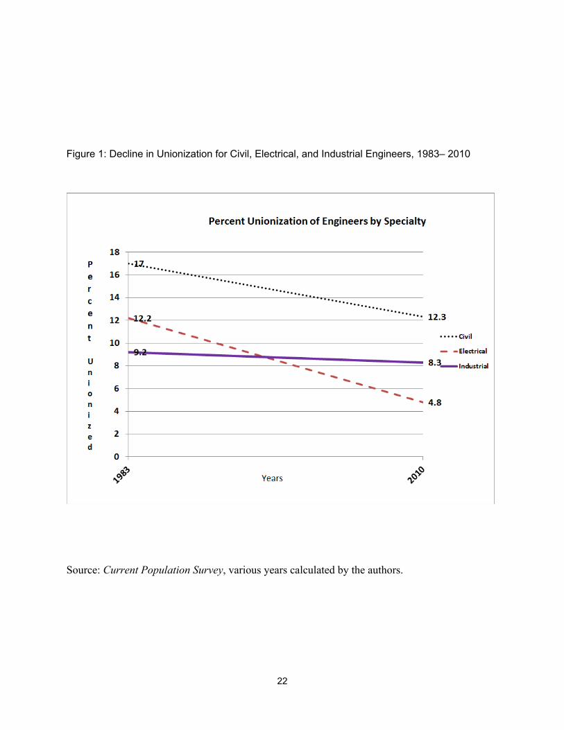
trends. Figure 1 shows the decline in unionization for civil, electrical, and industrial engineers

from 1983 to 2010. The steepest dip was for electrical engineers, where unionization declined

from about 12.2 percent in 1983 to 4.8 percent in 2010. The smallest decline was for industrial

engineers, whose rates of unionization declined from 9.2 percent to 8.3 percent over the same

time period. We will focus our analysis on these engineering specialties for this paper, since

they represent a continuum of more to less regulated specialties in engineering.

Since occupational regulation has many forms, describing its various types is

worthwhile. The occupational regulation of engineers in the United States generally takes three

forms. The least restrictive form is registration, in which individuals file their names, addresses,

and qualifications with a government agency before practicing their occupation. The registration

process may include posting a bond or filing a fee. In contrast, certification permits any person to

perform the relevant tasks, but the government—or sometimes a private, nonprofit agency—

administers an examination or other method to determine qualifications and certifies those who

3

have achieved the level of skill and knowledge for certification. For example, travel agents and

car mechanics are generally certified but not licensed. The toughest form of regulation is

licensure; this form of regulation is often referred to as “the right to practice.” Under licensure

laws, working in an occupation for compensation without first meeting government standards is

illegal. Our analysis provides a first look at the role of occupational licensing, rather than the

other two forms of governmental regulation in the labor market for engineers in the United

States.

We examine the role for occupational licensing in the labor market for engineers from

2001 through 2012. Initially, we present the evolution and anatomy of occupational licensing for

engineers. Next, we present a theory of licensing and show how this form of regulation leads to

wages dropping to the competitive wage as the licensing authority increases the supply of

practitioners. In the following section, we show the data for the analysis and present the growth

of regulation for the three types of engineers in our data set. Next, we present our empirical

analysis for three large specialties in engineering—civil, electrical, and industrial—when

variations in occupational licensing characteristics such as examinations and pass rates are

included. In the final section, we summarize our results.

The theoretical model shows that government-granted licenses to protect the public can

also lead to rents for the members of the occupation. As more individuals are allowed into the

occupation by the planner, wages fall. To the extent that regulation reduces innovation and that

unregulated members of the occupation can do higher wage tasks, regulation may diminish

wages. The estimates in our models are small for the labor market effects of licensing, and they

depend on the requirements and the engineering specialty examined. Also, some evidence

indicates that some licensing requirements influence the number of hours worked by engineering

4

specialty. The studies of the influence of licensing statutes on labor market outcomes perhaps

need better data on individuals who have a license rather than just state licensing coverage, since

coverage biases downward the influence of this type of regulation (Gittleman and Kleiner, 2013).

In this study we focus on licensing coverage rather than attainment, since determining attainment

is possible only when individual data explicitly ask whether an individual was licensed.

The Evolution and Anatomy of Licensing for Engineers

Similar to other occupations that eventually became licensed, such as dentists and nurses,

the government regulation of engineers began in the early 1900s (Council of State Governments,

1952). The first state to pass a licensure law was Wyoming in 1907. At the time, Wyoming

engineers were concerned with water speculators who lacked the qualifications or experience of

trained engineers but nonetheless used the term “engineer.” The law was passed so that “all the

surveying and engineering pertaining to irrigation works should be properly done” (Russell and

Stouffer, 2003, p.1). The American Society of Civil Engineers (ASCE) supported this piece of

legislation, but otherwise resisted the notion of state-controlled licensing. After 1910, many civil

engineering associations supported the concept of state licensing in order to control specific

aspects of the practice that would be regulated. The ASCE promulgated a model law for

licensure in 1910. This shift in policy also helped the occupation of civil engineering to be

consistent with regulations that were being developed in other professions such as medicine and

law, which had already accepted licensure (Haber, 1991; Pfatteicher, 1996).

Around 1920, the National Council of State Boards of Engineering Examiners was

formed to work for licensure in every state, help enforce regulations, and ensure appropriate

levels of experience and education for professional practice. This organization evolved into the

National Council of Examiners for Engineering and Surveying (NCEES). As more states adopted

5

regulations for professional practice, these engineering associations also became involved in

advocating for the standardization of engineering curricula in professional schools and

universities. It took nearly 45 years for all 50 states to require licensure for the practice of civil

engineering, although these licenses were required only for certain types of tasks that engineers

perform.

In contrast, chemical, electrical, mechanical, and petroleum engineering were recognized

as title holders and were covered by licensing following World War II. In the 1960s, industrial

engineering was recognized as a title branch and was also regulated. Table 1 shows the

percentage of engineers licensed by specialty in the United States, according to the National

Council of Examiners for Engineering and Surveying (NCEES) in 1995 and from the Survey of

Income and Program Participation (SIPP) for 2012. Civil engineering was by far the most

regulated branch of engineering, with more than 44 percent of those practicing being licensed in

1995. This value declined to 31 percent in the SIPP in 2012. As the estimates in Table 1 show,

about 9 percent of the electrical engineers were licensed in the mid-1990s and in 2012, and about

8 to 9 percent of industrial engineers were licensed in the mid 1990s and in 2012. This suggests

large variance in the amount of regulation in the occupation of engineering. Moreover, the vast

majority of engineers are covered by licensing statutes, but do not attain a license.

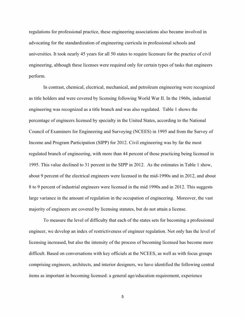
To measure the level of difficulty that each of the states sets for becoming a professional

engineer, we develop an index of restrictiveness of engineer regulation. Not only has the level of

licensing increased, but also the intensity of the process of becoming licensed has become more

difficult. Based on conversations with key officials at the NCEES, as well as with focus groups

comprising engineers, architects, and interior designers, we have identified the following central

items as important in becoming licensed: a general age/education requirement, experience

6

requirements, a written exam, a practical performance exam, a specific engineering specialty

exam, reciprocity requirements from other states, and a continuing education requirement.1

These elements are the basis of an index of the rigor of the licensing process, in addition to the

type of licensing. Using this index, we can trace the evolution of the intensity of the licensing

index in the period 1995–2012. Table 3 summarizes the index of licensing regulations for

engineers. The results show a slight upward movement in the mean values and a narrower spread

in the variance of the licensing provisions across states. Occupational licensing is growing

among states, and its provisions to enter and maintain good standing as a licensed professional

engineer are becoming more stringent.

The nation's umbrella engineering licensing body embraced a so-called Model Rule that

would extend by 30 the number of extra credit-hours BS-degreed engineers must have to gain a

professional license, but no state licensing board has made it a reality. However, the deadline for

the professional association is in 2020. The goals of the licensing groups are to increase the

status of engineers. For example, Blaine Leonard, former ASCE president and supporter of the

increased requirements for becoming a licensed engineer, stated the following: "If we want to

meet challenges and be prepared to protect the public, engineers need more depth of knowledge.

You can't get it in programs under pressure." Proponents would like to see engineering attain the

same professional status as medicine and accounting. The National Academy of Engineering and

the National Society of Professional Engineers support the idea,” (Rubin and Tuchman, 2012).

Basic Theory

1We met and discussed with officials at the Minnesota Board of Architecture, Engineering, Land Surveying Landscape Architecture, Geoscience and Interior Design (AELSLAGID) regarding key criteria for licensing in that state and with several licensed engineers in Minnesota, Arizona, and California.

7

To provide a theoretical context for our empirical work, we first review a model of the

influence of licensing on the supply of labor. In the following section, we focus on the demand

for labor and how government can be an important factor within a licensing model. The analysis

of wage determination under licensing in engineering builds on work by Perloff’s (1980) work

on the influence of licensing laws on wage changes in the construction industry. The basic model

posits that market forces are largely responsible for wage determination and that demand for

work is highly cyclical. This approach would also apply to the engineering labor market. Perloff

presents two cases. In the first, there are no costs to shifting across industries so that labor supply

is completely elastic at the opportunity wage. In this case, the increase in the demand for work

would have little effect on wages, since workers would flow between varying industries. The

introduction of a licensing law renders the supply of labor inelastic. In this case, labor cannot

flow between the sectors so that variations in demand would be reflected in the wage. In his

empirical work, Perloff shows that for electricians, more so than for either laborers or plumbers,

state regulations make the supply curve highly inelastic. Consequently, the ability of a state to

limit entry or impose major costs on entry through licensing would enhance the occupation’s

ability to raise wages. We would expect that a similar approach would apply to the market for

engineers, with more inelastic supply curves for civil engineers relative to electrical and

industrial engineers.

Unlike the work that has been developed on the supply side, relatively little analysis has

been done on how degrees of restriction of labor supply with occupational licensing influence

wages and the amount of work, and how such restrictions of supply can make the labor market

deviate from a competitive market. Our model focuses on the supply restriction of labor, and

8

we develop a general model that we will apply to the regulation of engineers. We develop a

model as follows:

Let

n

iiqQ

1

, where qi is each engineer’s work output, n is the number of engineers in the

market, and Q is the total quantity of supply. Each engineer’s monetary utility function is

)()( iiii qDQPqU , where D denotes the engineer’s disutility and P is the price of work output

(i.e. wage). The first-order condition for utility maximization is 0)(')(')( QPqqDQP iii .

From the above equation, we have

QQP

PQ

q

P

qDQPi

ii

)('

)(')( (1), where Qqi / is

engineer i's market share, and QQP

P

)(' is the elasticity of demand. Thus, the gap between

price and marginal disutility is proportional to the engineer’s market share and inversely

proportional to the elasticity of demand. Price exceeds the engineer’s marginal disutility as long

as α is non-zero. The larger the difference, the more prices deviate from the socially efficient

price.

For instance, for the symmetric case in which every engineer has the same output, with

linear demand, P(Q) = 1 - aQ for all i, and the convex disutility function being 2cqbqD . We

assume that a, b, c are greater than zero, so that the demand is inversely related to price and the

disutility is a convex function. The first-order condition of the engineer’s utility maximization

becomes 021 ii aqcqbaQ . The equilibrium is symmetric for this model: Q = nq, where

9

q is the output per engineer. Hence, we obtain acan

bq

2

1 (2). The market price is

acan

acbbp

2

)2)(1( (3), and each engineer’s utility is 2

2

)2(

)()1(

acan

cabU

(4).

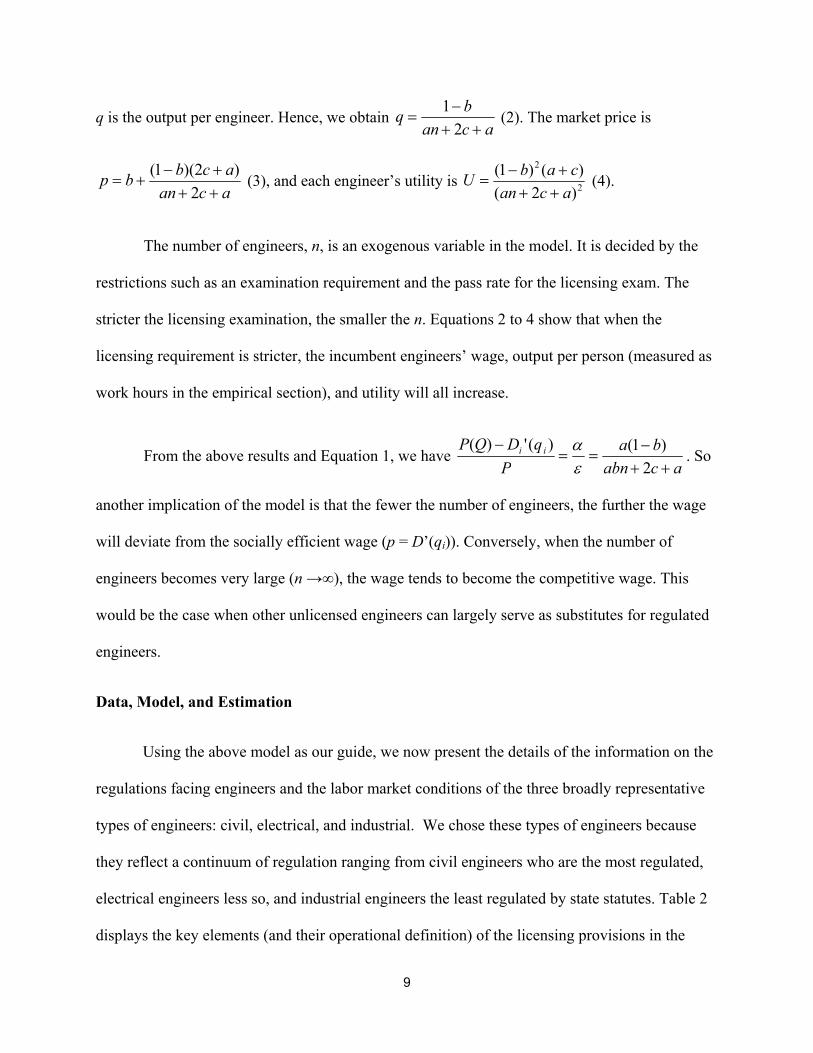
The number of engineers, n, is an exogenous variable in the model. It is decided by the

restrictions such as an examination requirement and the pass rate for the licensing exam. The

stricter the licensing examination, the smaller the n. Equations 2 to 4 show that when the

licensing requirement is stricter, the incumbent engineers’ wage, output per person (measured as

work hours in the empirical section), and utility will all increase.

From the above results and Equation 1, we have acabn

ba

P

qDQP ii

2

)1()(')(

. So

another implication of the model is that the fewer the number of engineers, the further the wage

will deviate from the socially efficient wage (p = D’(qi)). Conversely, when the number of

engineers becomes very large (n →∞), the wage tends to become the competitive wage. This

would be the case when other unlicensed engineers can largely serve as substitutes for regulated

engineers.

Data, Model, and Estimation

Using the above model as our guide, we now present the details of the information on the

regulations facing engineers and the labor market conditions of the three broadly representative

types of engineers: civil, electrical, and industrial. We chose these types of engineers because

they reflect a continuum of regulation ranging from civil engineers who are the most regulated,

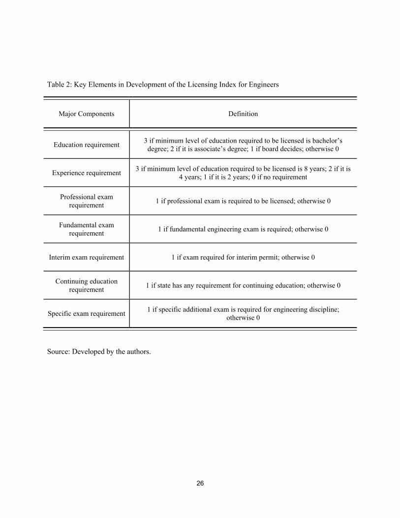
electrical engineers less so, and industrial engineers the least regulated by state statutes. Table 2

displays the key elements (and their operational definition) of the licensing provisions in the

10

statutes and administrative provisions that we plan to examine for each of the states in our

sample for engineers.

Table 3 shows the yearly growth in the occupational licensing statutes index over the

period 1995–2012. The results indicate that the occupation experienced growth in regulations

governing entry and training requirements. The level of the index or the number of items

included in the state level measure grew from 6.94 to 7.25, or by about 4 percent over this time

period. This reflects the intensity of the growth of requirements to enter and maintain the status

as a licensed engineer. Further, the standard deviation declined by almost 23 percent, suggesting

greater standardization of the requirements for licensing across states and over time.

Table 4 shows the relative ranking of the states that have the highest and lowest values in

the index. We also developed values that were established through an expert systems focus

group approach to test the sensitivity of the results to alternative methods of evaluation. In this

approach, an engineering student and a law student were given the data and asked to rank the

states based on issues that were personally important to them as professionals in their respective

fields. There was a high degree of consistency for the empirical and qualitative approaches. For

many states, we were able to obtain the pass rates for the licensing examination for engineers2.

Figure 2 shows the states and time trend in years for which we were able to obtain from the

licensing boards of each of the states that posted their overall engineering pass rates.3 The plots

in the figure show that California has the lowest steady-state pass rate for the engineering exam,

averaging about 40 percent per year. In contrast, the pass rate for the licensing of engineers in

2 The links to the boards were available at http://ncees.org/licensing-boards. We went to the data from each state to obtain pass rates. 3 The Tables A1 and A2 in the Appendix show the influence of the variations in the pass rates and the influence of the statutory provisions of test requirements on both wages and hours of work for a limited number of states in which the data were available.

11

Idaho is well above 80 percent. Unfortunately, no systematic national estimates could be

developed because of the state data limitations over time and across states.

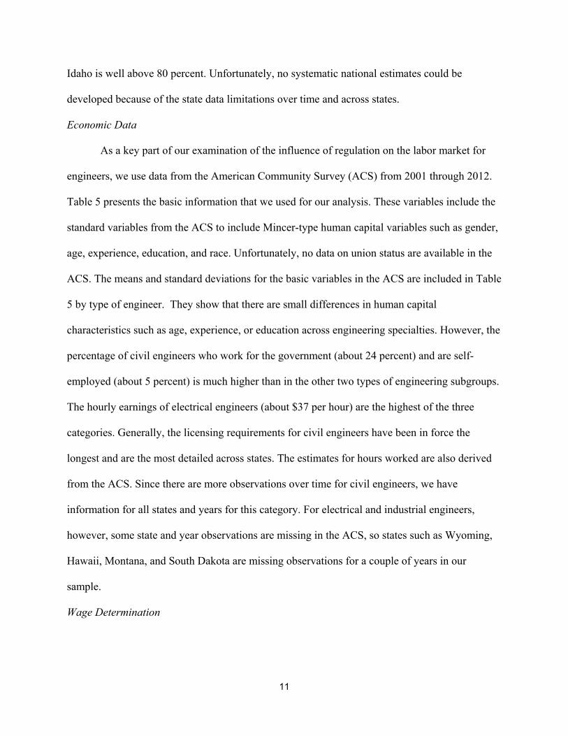
Economic Data

As a key part of our examination of the influence of regulation on the labor market for

engineers, we use data from the American Community Survey (ACS) from 2001 through 2012.

Table 5 presents the basic information that we used for our analysis. These variables include the

standard variables from the ACS to include Mincer-type human capital variables such as gender,

age, experience, education, and race. Unfortunately, no data on union status are available in the

ACS. The means and standard deviations for the basic variables in the ACS are included in Table

5 by type of engineer. They show that there are small differences in human capital

characteristics such as age, experience, or education across engineering specialties. However, the

percentage of civil engineers who work for the government (about 24 percent) and are self-

employed (about 5 percent) is much higher than in the other two types of engineering subgroups.

The hourly earnings of electrical engineers (about $37 per hour) are the highest of the three

categories. Generally, the licensing requirements for civil engineers have been in force the

longest and are the most detailed across states. The estimates for hours worked are also derived

from the ACS. Since there are more observations over time for civil engineers, we have

information for all states and years for this category. For electrical and industrial engineers,

however, some state and year observations are missing in the ACS, so states such as Wyoming,

Hawaii, Montana, and South Dakota are missing observations for a couple of years in our

sample.

Wage Determination

12

Our empirical strategy is to first examine the three categories of engineers—civil,

electrical, and industrial—that may vary greatly by the type of regulation that influences their

ability to find employment. We estimate the model using all engineers in the categories together

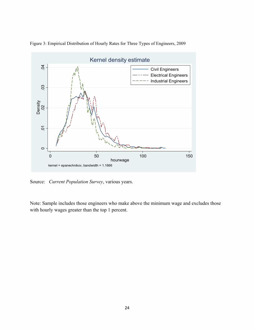
and then estimate wage equations for each group separately. In Figure 3 we show kernel density

plots for the three types of engineers in our study. The results show that electrical engineers have

the highest mean value for wages and the widest distribution of earnings among the three types

of engineers we study, but industrial engineers have the lowest mean value.

Our basic model uses an earnings function and compares the three types of engineers (the

least regulated one—industrial engineers—is the excluded category). Our basic model is of the

following form:

1) ln( ,

where Earningsist is the hourly earnings of engineer i at state s in year t; Tsti is the type of

engineer (civil, electrical, or industrial) for person i’s state s in year t; Rsti is the occupational

licensing regulations (and its components) in person i’s state s in year t; Xist is the vector that

includes covariates measuring characteristics of each person; δ and θ are state and year fixed

effects, respectively; and εist is the error term in our panel data.4

The model is a basic fixed effects approach that can also be viewed as a generalization of

the conventional two-group two-period difference-in-difference model.5 The estimates presented

in the tables show the results for both a traditional panel estimate using individuals as the unit of

observation of the role of regulation on wage determination and a two-stage estimation

procedure. For the two-stage procedure, the first stage is developed by estimating a model of

4 The use of a Rasch measure resulted in no basic effect of regulation on either wage determination or hours worked; consequently, we use the summated rating scale. 5 We also included time-varying state-level controls, such as the state median household income, but found that they have no explanatory power. Consequently, we do not show the results in this paper.

13

individual-level outcomes on covariates and a full set of state x (×) time fixed effects. The

coefficients on the state x (×) time fixed effects represent state x time mean outcomes that have

been purged of the variation associated with the within-cell variation in the covariates. In the

second stage, these adjusted cell level means are estimates on the policy variables and fixed

effects. The two-step approach is a way of performing aggregation while still allowing for

adjustment of individual-level covariates, which is a limitation of the pure aggregation. The basic

panel estimates include individual covariates as well as state and year fixed effects.6

Table 6 shows estimates from the model developed from the overall licensing index on

wage determination using both the individual observations and the two- level analyses with

controls. Since the index is an imprecise measurement of regulation, we develop a relative

measure of regulation of high, medium, and low levels of regulation using our index. We then

compare the highest levels of regulation relative to the low and medium ones. The first column

shows the basic bivariate relationship between having the most restrictive licensing statutes and

wage determination with the full sample of the ACS. The basic relationship shows a statistically

significant 2 percent effect7. However, in the second column when human capital and state

specific covariates are included, the estimates are still positive but small and not statistically

significant. In examining the various engineering specializations in columns 3 through 8, we can

see that there is some variation. For example, the bivariate estimates for civil engineers show a

positive but small influence of being in a state with the most stringent regulations in the first

stage, but no effect in the second stage. Similarly, for both electrical and industrial engineers,

the engineering regulations have a small but positive effect in the first stage bivariate estimates,

6 The standard errors for these models were computed using a Huber-White covariance matrix that allowed for clustering at the state level. 7 We also estimated models that examined the influence of tougher licensing before and after the great recession of 2008, and found results similar to those presented in Tables 6, 7, 9 and 10.

14

but no influence in the second stage results. The significant estimates range from a high of 4

percent with no covariates for industrial engineers with no covariates to no effect in the fully

specified model. The categorical specifications show regulation for engineers has a small effect

that is close to zero. This is not unlike some of the specifications of the influence of unions on

wage determination for other professional organizations (Lewis, 1986). Moreover, we only have

estimates of licensing coverage and not those who have attained a license, which may bias our

results downward (Gittleman and Kleiner, 2013). However, licensing requirements may also

have effects on the supply of hours to the market.

The models developed for hours of work use approaches similar to the ones developed

for our wage equation models. In a similar manner, we examine employment growth for each of

the categories of engineers from 2001 to 2012. The basic model is of the following form:

ln

where Employmentist is hours of work per week per engineer in state s in time period t for

individual i; Tist is the type of engineer at state s in time period t for individual i; Rst is the

regulation measure and its components at state s in time period t; the vector Xst includes

covariates measuring economic and human capital characteristics within each state; δs and θt are

state and year fixed effects, respectively; and €ist s the error term.

Table 7 gives the basic results for the impact of the licensing index on hours of work

supplied by engineers using the specified model using categorical measures of regulation of high

relative to low or medium. The results are consistent in showing that regulation is associated

with an increase in hours worked by about 1 percent in the bivariate estimates, but no effect

when the two-level analyses is implemented with standard human capital controls. If regulation

is effective in restricting the supply of new entrants to some extent, then those in the occupation

15

are likely to work more hours. The results in Table 7 are consistent with this hypothesis, but the

magnitudes are small.

Although the categorical transformation of the overall index does not show much effect

on the key labor market variables of wages and hours worked, perhaps several of the individual

components of the licensing index may influence wages and hours worked. The use of an

examination to determine the impact of this variable on wage determination has been used in

other studies (Kleiner and Kudrle, 2000; Kleiner and Krueger, 2013). Through the examination

process and the establishment of higher standards, access to and supply of engineers can be

reduced, and if demand remains constant, wages can increase. Moreover, the pass rate for the

engineering exam also may limit the entry of new engineers and drive up wages for engineers.

In Table 8 we list the states that require a professional exam for each specific type of

licensing examination. In order to become licensed, engineers usually take a fundamental or first

exam, the basic step toward becoming a licensed engineer. This exam is often administered to

engineers just prior to their finishing undergraduate studies. The professional exam, in contrast,

covers general engineering practices and is usually given after engineers have been practicing for

four or more years. It is the final stage of licensing coverage for entry into the regulated part of

the occupation. Table 8 shows that Ohio and Arkansas adopted a professional exam in 2002 and

2009, respectively; they serve as basis for a difference-in-difference analysis. The difference-in-

difference model is relative to Ohio and Arkansas, which were the states that changed their

regulatory statutes for exams over the time period of our analysis.

In order to provide sensitivity analysis for our previous estimates and include the

estimates for an additional regulatory requirement, we include whether there is a professional

exam requirement to become licensed. Table 9 shows the estimates on wage and hours using

16

seemingly unrelated regression (SUR) methods for the influence of having a professional exam

requirement as part of the licensing requirement. Since only two states changed the exam

requirements during the period under study, we used this method as an additional sensitivity test

of our estimates. Panel A shows the results when engineers are categorized by type of

engineering field: civil, electrical, and industrial. In Panel B we estimate the model for all the

engineers in our sample. Those results are consistent with the general results shown in Table 6,

7, and 8 and show only a small coefficient size for this requirement and varying levels of

significance, based on the type of engineering specialty and the labor market outcome variable

selected, which was hourly wages or hours worked.

In Table 10, we examine whether the lagged professional exam requirement variable may

have influenced economic factors. Using the lagged professional licensing requirement and

current economic data starting in 2001 through 2012, the table shows that these results are

consistent in displaying a mixed to minor influence on wage determination. At least for

licensing coverage, which is what our data allow us to measure, occupational licensing has a

small influence on wage determination for civil engineers, but has a mixed influence on other

engineering specialties. This may reflect the fact that the attainment of a license matters more

with respect to wage determination, rather than the passage of a law regulating an occupation

that is largely unregulated by the government (Gittleman and Kleiner, 2013). Even though H.

Gregg Lewis finds that being represented by a union raises wages by about 15 percent in

aggregate, for many occupations such as hospital workers and well-educated male workers, the

influence of unions is either zero or even slightly negative (Lewis, 1986). Similarly, for civil

engineers, who are more heavily licensed, tougher regulations may not enhance their earnings,

17

perhaps because unregulated workers are able to be more innovative and create new markets

relative to engineers who have their work standardized by the government (Friedman, 1962).

Conclusions

Our paper presents the first comprehensive analysis of the role of occupational licensing

requirements on the labor market for civil, electrical, and industrial engineers. These groups of

engineers represent the largest number of engineers that are covered by occupational licensing

statutes in the United States. We initially trace the historical evolution of licensing for engineers.

Second, we present a theoretical rationale for the role of government in the labor market for the

occupation. In the model, the government’s ability to control supply through licensing

restrictions and the pass rate limits the number of engineers, which may drive up wages. These

results are useful for informing the empirical models for engineers.

In the empirical section, we show that licensing for these occupations has grown

somewhat more rigorous during the period 2001–2012. We then estimate a panel data model for

the engineers in our sample using the ACS. Our estimates show a small influence of occupational

licensing on both wages and employment in a variety of specifications and sensitivity analysis

tests. In the U.S. economy, if engineers achieve the goal of their professional association of

more rigid requirements, and a longer time to become an engineer, the growth of regulation of

the occupation may reduce customer access to engineers and slow down the ability of builders

and manufacturers to use regulated engineering services. Our study provides a first look at these

issues. Exploring the potential issue of selection across engineering specialties, and using more

detailed analysis such as the use of discontinuities when the passage of more rigorous laws

occurs, may provide more refined or precise estimates and examples of the role of regulation in

18

the market for engineers. Further, a more thorough analysis would include individuals who have

attained a license rather than licensing coverage, and these data would allow us to obtain a better

measure of the influence of occupational licensing on those who chose to get the credential to

legally do certain engineering tasks.

19

References

Brinegar, P., and K. Schmitt. 1992. “State Occupational and Professional Licensure.” In The

Book of the States, 1992–1993. Lexington, KY: Council of State Governments, 567–80.

Council of State Governments. 1952. Occupational Licensing Legislation in the States. Chicago:

Council of State Governments.

Dunlop, J. T. 1958. Industrial Relations Systems. New York: Holt.

Folk, H. 1970. The Shortage of Scientists and Engineers. Lexington, MA: Lexington-Lexington

Press.

Freeman, R. B. 1976. “A Cobweb Model of the Supply and Starting Salary of New Engineers.”

Industrial and Labor Relations Review, 29(2): 236–48.

Friedman, Milton, 1962. Capitalism and Freedom. Chicago: University of Chicago Press.

Gittleman, M., and M. M. Kleiner. 2013. “Wage Effects of Unionization and Occupational

Licensing Coverage in the United States.” Working Paper no. 19061, National Bureau of

Economic Research.

Haber, S. 1991. The Quest for Authority and Honor in the American Professions, 1750–1900.

Chicago: University of Chicago Press.

Hansen, W. L. 1961. "The Shortage of Engineers." Review of Economics and Statistics, 43(3):

251–56.

20

Hirsch, B. T., and D. A. Macpherson. 2011. "Union Membership and Coverage Database from

the Current Population Survey," September. Available at http://www.unionstats.com.

Kleiner, M. M. 2006. Licensing Occupations: Ensuring Quality or Restricting Competition?

Kalamazoo, MI: W. E. Upjohn Institute.

Kleiner, M.M. 2013. Stages of Occupational Regulation: Analysis of Case Studies. Kalamazoo,

MI: W. E. Upjohn Institute.

Kleiner, M. M., and A. B. Krueger. 2013. “Analyzing the Extent and Influence of Occupational

Licensing on the Labor Market.” Journal of Labor Economics, 31(2): S173–202.

Kleiner, M., and R. Kudrle. 2000. “Does Regulation Affect Economic Outcomes? The Case of

Dentistry.” Journal of Law and Economics, 43(2): 547–82.

Kleiner, M., and R. Todd. 2009. “Mortgage Broker Regulations That Matter: Analyzing

Earnings, Employment, and Outcomes for Consumers.” In Studies of Labor Market

Intermediation, ed. D. Autor. Chicago: University of Chicago Press.

Lewis, H. Gregg. 1986. Union Relative Wage Effects: A Survey. Chicago: University of Chicago

Press.

Perloff, J. M. 1980. “The Impact of Licensing Laws on Wage Changes in the Construction

Industry.” Journal of Law and Economics, 23(2): 409–28.

Pfatteicher, S.K.A. 1996. “Death by Design: Ethics, Responsibility and Failure in the American

Civil Engineering Community, 1852–1986.” Ph.D. diss., University of Wisconsin–

Madison.

21

Princeton Data Improvement Initiative (PDII). 2008. Available at

http://www.krueger.princeton.edu/PDIIMAIN2.htm.

Rubin, D. K. and J. L. Tuchman, 2012. “Professional Engineers' License Debate

Grows in Intensity”, Engineering News-Record, October 17, p.1 -2.

Russell, J., and W. B. Stouffer. 2003. “Change Takes Time:

The History of Licensure and Continuing Professional Competency.” Report, American

Society of Civil Engineers, p.7. Available at

http://www.asce.org/uploadedFiles/Landing_Pages/Leadership_and_Management/The

%20History%20of%20Licensure%20and%20Continuing%20Professional%20Compete

ncy_FINAL.pdf.

U.S. Department of Labor, Bureau of Labor Statistics. 2013. Current Population Survey.

22

Figure 1: Decline in Unionization for Civil, Electrical, and Industrial Engineers, 1983– 2010

Source: Current Population Survey, various years calculated by the authors.

23

Figure 2: Engineering Exam Pass Rates by State

2040

6080

2040

6080

2040

6080

2040

6080

2040

6080

2040

6080

2040

6080

2040

6080

2040

6080

2040

6080

2040

6080

2040

6080

2040

6080

2040

6080

2040

6080

2040

6080

2040

6080

2000 2005 2010 2000 2005 2010 2000 2005 2010 2000 2005 2010 2000 2005 2010

2000 2005 2010 2000 2005 2010 2000 2005 2010 2000 2005 2010 2000 2005 2010

2000 2005 2010 2000 2005 2010 2000 2005 2010 2000 2005 2010 2000 2005 2010

2000 2005 2010 2000 2005 2010

Alabama Alaska California Colorado Idaho

Kansas Kentucky Minnesota Mississippi Missouri

New Mexico Oklahoma Oregon Tennessee Texas

Virginia Washington

pas

s ra

te

yearGraphs by State

Sources: The pass rate data for those states that post this information was obtained from http://ncees.org/licensing-boards/. In addition, we contacted the state boards to obtain pass rates for engineers for others not posted.

24

Figure 3: Empirical Distribution of Hourly Rates for Three Types of Engineers, 2009 0

.01

.02

.03

.04

Den

sity

0 50 100 150hourwage

Civil Engineers

Electrical EngineersIndustrial Engineers

kernel = epanechnikov, bandwidth = 1.1666

Kernel density estimate

Source: Current Population Survey, various years.

Note: Sample includes those engineers who make above the minimum wage and excludes those with hourly wages greater than the top 1 percent.

25

Table 1: Percentage of Engineers Licensed by Specialty, 1995* and 2012**

Engineering Discipline

Percentage Licensed 1995

Percentage Licensed 2012

Civil 44 31 Electrical 9 9 Industrial 8 9

*Source: Paul Taylor, NCEES Licensure Bulletin, December 1995. ** Survey of Income and Program Participation, 2013

26

Table 2: Key Elements in Development of the Licensing Index for Engineers

Major Components Definition

Education requirement 3 if minimum level of education required to be licensed is bachelor’s degree; 2 if it is associate’s degree; 1 if board decides; otherwise 0

Experience requirement 3 if minimum level of education required to be licensed is 8 years; 2 if it is

4 years; 1 if it is 2 years; 0 if no requirement

Professional exam requirement

1 if professional exam is required to be licensed; otherwise 0

Fundamental exam requirement

1 if fundamental engineering exam is required; otherwise 0

Interim exam requirement 1 if exam required for interim permit; otherwise 0

Continuing education requirement

1 if state has any requirement for continuing education; otherwise 0

Specific exam requirement 1 if specific additional exam is required for engineering discipline;

otherwise 0

Source: Developed by the authors.

27

Table 3: Growth of Occupational Licensing Intensity over Time

Year No. of state Mean Std. Dev. Min Max

1995 51 6.94 2.04 0.00 9.00

1996 51 6.86 2.03 0.00 9.00

1997 51 6.89 1.86 0.00 9.00

1998 51 7.08 1.71 0.00 9.00

1999 51 7.08 1.71 0.00 9.00

2000 51 7.06 1.70 0.00 9.00

2001 51 7.06 1.70 0.00 9.00

2002 51 7.06 1.70 0.00 9.00

2003 51 7.06 1.70 0.00 9.00

2004 51 7.08 1.72 0.00 9.00

2005 51 7.08 1.72 0.00 9.00

2006 51 7.08 1.72 0.00 9.00

2007 51 7.08 1.72 1.00 9.00

2008 51 7.08 1.72 1.00 9.00

2009 51 7.08 1.72 1.00 9.00

2010 51 7.25 1.59 1.00 9.00

2011 51 7.25 1.59 1.00 9.00

2012 51 7.25 1.58 1.00 9.00

Note: Index is the summated rating value of the key provisions for licensing engineers as noted in Table 2 tabulated by the authors.

28

Table 4: Regulation Rankings of Top and Bottom States by Restrictiveness of Licensing, 2009

Top States Index Bottom States Index

Pennsylvania 9 Virginia 1

Georgia 9 Minnesota 3

Texas 9 South Dakota 4

Illinois 9 DC 5

Arizona 9 Delaware 5

Colorado 9 Connecticut 5

29

Table 5: Key Variables for Engineers in the ACS, 2001–2012

Civil Engineers Electrical Engineers Industrial Engineers

Mean S.D. Mean S.D. Mean S.D.

Age 43.05 11.27 43.48 10.65 43.76 10.83

Schooling (in Year) 16.00 1.67 16.21 1.66 15.70 1.66 Gender (Male:1;

Female:0) 0.74 0.44 0.91 0.28 0.81 0.39

Married (Married:1; Not Married:0)

0.73 0.45 0.76 0.43 0.74 0.44

Experience (in Year) 21.05 11.40 21.28 10.89 22.06 11.11

Experience-Squared 572.88 495.33 571.25 473.94 610.37 492.57 White (White:1;

Others:0) 0.84 0.36 0.79 0.41 0.87 0.34

Black (Black:1; Others:0)

0.05 0.22 0.04 0.20 0.04 0.19

Citizen (U.S. Citizen:1; Others:0)

0.95 0.21 0.91 0.29 0.94 0.23

Work for For-Profit (Yes:1; No:0)

0.70 0.64 0.88 0.32 0.93 0.26

Work for Not-for-Profit (Yes:1; No:0)

0.04 0.49 0.02 0.14 0.01 0.11

Work for Government (Yes:1; No:0)

0.24 0.62 0.09 0.28 0.05 0.22

Self-employment (Yes:1; No:0)

0.05 0.49 0.01 0.12 0.01 0.08

Hourly Earnings (in 2009 dollars)

34.61 21.20 37.47 18.41 30.35 14.72

Source: American Community Survey.

30

Table 6: Influence of Statutory Rank Index on Wage Determination: High Relative to Medium and Low (1) (2) (3) (4) (5) (6) (7) (8) One- level

Analysis Two- level

Analysis

One- level

Analysis

Two- level

Analysis

One- level

Analysis

Two- level

Analysis

One- level

Analysis

Two- level

Analysis Sample All All Civil Civil Electrical Electrical Industrial Industrial Highest rank 0.024*** 0.007 0.013*** -0.008 0.023*** 0.026 0.042*** -0.014 (0.000) (0.016) (0.001) (0.023) (0.001) (0.028) (0.001) (0.034) Observations 7,231,650 612 3,404,866 612 2,300,115 605 1,526,669 580 R-squared 0.000 0.852 0.000 0.715 0.000 0.706 0.000 0.580 Basic control NO YES NO YES NO YES NO YES Year fixed NO YES NO YES NO YES NO YES State fixed NO YES NO YES NO YES NO YES

Note: Estimated with age, schooling in years, gender, marital status, experience, experience-squared, race, U.S. citizenship, for profit sector, and self-employment. Two-stage regressions are weighted by the number of engineers. The second-stage estimates are aggregate state-level estimates of hours worked calculated from the predicted hours worked individual model, which are then aggregated to the state level. The ACS sample uses individuals who earn less than $250 per hour and who are college graduates. Standard errors are in parentheses.

*** p<0.01, ** p<0.05, * p<0.1

31

Table 7: Influence of Statutory Rank Index on Hours Worked: High Relative to Medium and Low

(1) (2) (3) (4) (5) (6) (7) (8) One-

level Analysis

Two- level

Analysis

One- level

Analysis

Two- level

Analysis

One- level

Analysis

Two- level

Analysis

One- level

Analysis

Two- level

AnalysisSample All All Civil Civil Electrical Electrical Industrial Industrial Highest rank 0.010*** 0.009 0.010*** 0.010 0.015*** 0.012 0.005*** 0.008 (0.000) (0.006) (0.000) (0.008) (0.000) (0.009) (0.000) (0.011) Observations 7,231,650 612 3,404,866 612 2,300,115 605 1,526,669 580 R-squared 0.001 0.335 0.001 0.202 0.002 0.216 0.000 0.196 Basic control NO YES NO YES NO YES NO YES Year fixed NO YES NO YES NO YES NO YES State fixed NO YES NO YES NO YES NO YES


*** p<0.01, ** p<0.05, * p<0.1

32

Table 8: State Professional Exam Requirements for Licensure of Engineers, 2001–2012

Professional exam required No professional exam required

Changer (year of change)

Alabama Ohio (2002)

Alaska Arizona

Arkansas (2009)

California Hawaii

Colorado Missouri

Connecticut New Hampshire

Delaware New Jersey

District of Columbia New Mexico

Florida Oregon

Georgia South Dakota

Idaho Utah

Illinois Virginia

Indiana Iowa

Washington

Kansas Wisconsin

Kentucky Louisiana

Wyoming

Maine

Maryland

Massachusetts

Michigan Minnesota Mississippi

Montana Nebraska

Nevada New York

North Carolina

North Dakota

Oklahoma

Pennsylvania

Rhode Island

South Carolina

Tennessee

Texas

Vermont

West Virginia

33

Table 9

Panel A: Effect of a Professional Exam on Wage and Hours Worked Using Seemingly Unrelated Regressions (SUR)

Sample Civil Engineers Electrical Engineers Industrial Engineers

(1) (2) (3) (4) (5) (6) (7) (8) (9) (10) (11) (12)

One Step Two step One Step Two step One Step Two step

VARIABLES Log of wage Log of Hours

worked

Log of wage

Log of Hours

worked

Log of wage Log of Hours

worked

Log of wage

Log of Hours

worked

Log of wage Log of Hours

worked

Log of wage

Hours worked

index_pe index_pe -0.002*** 0.003*** -0.146*** -0.057*** 0.003*** 0.006*** 0.042 0.012 -0.025*** -0.001** -0.143** -0.002 (0.001) (0.000) (0.048) (0.017) (0.001) (0.000) (0.060) (0.020) (0.001) (0.000) (0.071) (0.023) Constant 3.437*** 3.756*** 3.637*** 3.796*** 3.520*** 3.755*** 3.537*** 3.730*** 3.351*** 3.781*** 3.551*** 3.802***

Observations (0.001) (0.000) (0.056) (0.020) (0.001) (0.000) (0.068) (0.023) (0.001) (0.000) (0.081) (0.027) R-squared

Basic control Observations 3,404,866 3,404,866 612 612 2,300,115 2,300,115 605 605 1,526,669 1,526,669 580 580

Year fixed R-squared 0.000 0.000 0.719 0.219 0.000 0.000 0.706 0.209 0.000 0.000 0.583 0.168

State fixed Basic control NO NO YES YES NO NO YES YES NO NO YES YES Year fixed NO NO YES YES NO NO YES YES NO NO YES YES

State fixed NO NO YES YES NO NO YES YES NO NO YES YES

34

Panel B: Effect on Wage Using SUR for All Engineers

(1) (2) (3) (4)

ANALYSIS One Step Two Step

VARIABLES Log of wage Log of Hours work

Log of wage Log of Hours work

index_pe -0.006*** 0.004*** -0.107*** -0.022*

(0.000) (0.000) (0.034) (0.012)

Constant 3.446*** 3.760*** 3.571*** 3.775*** (0.000) (0.000) (0.039) (0.013)

Observations 7,231,650 7,231,650 612 612

R-squared 0.000 0.000 0.854 0.303

Basic control NO NO YES YES

Year fixed NO NO YES YES

State fixed NO NO YES YES

Note: Panels A and B were estimated with age, schooling in years, gender, marital status, experience, experience-squared, race, U.S. citizenship, for profit sector, and self-employment. Two-stage regressions are weighted by the number of engineers. The second-stage estimates are aggregate state-level estimates of hours worked calculated from the predicted hours worked individual model, which are then aggregated to the state level. The ACS sample uses individuals who earn less than $250 per hour and who are college graduates. Standard errors are in parentheses.

*** p<0.01, ** p<0.05, * p<0.1

35

Table 10: Influence of Lagged Professional Exam on Wages and Hours Worked, 2001–2012

Sample All Engineers Civil Engineers Electrical Engineers Industrial Engineers

(1) (2) (3) (4) (5) (6) (7) (8)

Analysis One- step Two- step One- step Two- step One- step Two- step One- step Two- step

Panel A: Dependent is log of hourly wage

Lag professional exam

0.000 -0.076** 0.003*** -0.066 0.008*** -0.004 -0.016*** -0.128**

(0.000) (0.030) (0.001) (0.043) (0.001) (0.053) (0.001) (0.063) Constant 3.440*** 3.564*** 3.433*** 3.558*** 3.515*** 3.589*** 3.343*** 3.493*** (0.000) (0.036) (0.001) (0.052) (0.001) (0.064) (0.001) (0.076) Observations 7,231,650 612 3,404,866 612 2,300,115 605 1,526,669 580 R-squared 0.000 0.853 0.000 0.716 0.000 0.706 0.000 0.583

Panel B: Dependent is log hours worked

Lag professional exam

0.004*** -0.011 0.003*** -0.037** 0.007*** 0.024 -0.001*** -0.010

(0.000) (0.010) (0.000) (0.016) (0.000) (0.018) (0.000) (0.021) Constant 3.761*** 3.763*** 3.756*** 3.772*** 3.754*** 3.717*** 3.782*** 3.807*** (0.000) (0.012) (0.000) (0.019) (0.000) (0.021) (0.000) (0.025) Observations 7,231,650 612 3,404,866 612 2,300,115 605 1,526,669 580 R-squared 0.000 0.300 0.000 0.213 0.000 0.211 0.000 0.168 Basic control NO YES NO YES NO YES NO YES

Year fixed NO YES NO YES NO YES NO YES

State fixed NO YES NO YES NO YES NO YES


*** p<0.01, ** p<0.05, * p<0.1

36

Appendices

Table A1: Influence of Professional Exams (PE) and Pass Rates on Wage Determination of Engineers

Sample All Engineers

Civil Engineers Electrical Engineers Industrial Engineers

ANALYSIS

(1)

One- Step

(2)

Two- Step

(3)

One- Step

(4)

Two- Step

(5)

One- Step

(6)

Two- Step

(7)

One- Step

(8)

Two- StepVARIABLES Log of

wage Log of wage

Log of wage

Log of wage

Log of wage

Log of wage

Log of wage

Log of wage

PE*Pass rate -0.008*** 0.000 -0.005*** 0.001 -0.013*** 0.000 -0.006*** 0.000 (0.000) (0.001) (0.000) (0.002) (0.000) (0.002) (0.000) (0.001) PE 0.452*** -0.040 0.251*** -0.044 0.744*** -0.027 0.320*** -0.066 (0.005) (0.048) (0.007) (0.092) (0.008) (0.096) (0.011) (0.074) Pass rate 0.004*** -0.001 0.002*** -0.001 0.008*** -0.000 0.003*** -0.000 (0.000) (0.001) (0.000) (0.001) (0.000) (0.001) (0.000) (0.001) Constant 3.210*** 3.345*** 3.340*** 3.307*** 3.051*** 3.418*** 3.156*** 3.295*** (0.005) (0.040) (0.007) (0.077) (0.008) (0.081) (0.011) (0.062) Observations 2,195,841 123 1,007,204 123 775,218 123 413,419 122 R-squared 0.009 0.976 0.004 0.918 0.019 0.924 0.004 0.940 Basic control NO YES NO YES NO YES NO YES Year fixed NO YES NO YES NO YES NO YES State fixed NO YES NO YES NO YES NO YES


*** p<0.01, ** p<0.05, * p<0.1

37

Table A2: Effect of Professional Exams (PE) and Pass Rates on Hours Worked


Civil Engineers

Electrical Engineers

Industrial Engineer

s

ANALYSIS

(1)

One- Step

(2)

Two- Step

(3)

One- Step

(4)

Two- Step

(5)

One- Step

(6)

Two- Step

(7)

One- Step

(8)

Two- Step

VARIABLES Hours Worked

Hours Worked

Hours Worked

Hours Worked

Hours Worked

Hours Worked

Hours Worked

Hours Worked

PE*Pass rate 0.000*** -0.000 0.001*** 0.000 -0.000*** -0.000 0.001*** -0.000 (0.000) (0.000) (0.000) (0.000) (0.000) (0.000) (0.000) (0.000) PE -0.018*** 0.016** -0.061*** 0.006 0.041*** 0.005 -0.033*** 0.023 (0.002) (0.007) (0.002) (0.010) (0.002) (0.015) (0.003) (0.014) Pass rate 0.000*** 0.000 -0.000*** 0.000 0.001*** 0.000* 0.000* -0.000 (0.000) (0.000) (0.000) (0.000) (0.000) (0.000) (0.000) (0.000) Constant 3.750*** 3.751*** 3.773*** 3.742*** 3.709*** 3.752*** 3.775*** 3.779*** (0.001) (0.006) (0.002) (0.008) (0.002) (0.013) (0.003) (0.012) Observations 2,195,841 123 1,007,204 123 775,218 123 413,419 122 R-squared 0.002 0.950 0.004 0.952 0.003 0.882 0.003 0.915 Basic control NO YES NO YES NO YES NO YES Year fixed NO YES NO YES NO YES NO YES State fixed NO YES NO YES NO YES NO YES


*** p<0.01, ** p<0.05, * p<0.1

38

Table A2: Effect of Pass Rates on Hours Worked (cont.)


Civil Engineers

Electrical Engineers

Industrial Engineers

ANALYSIS

(1)

One- Step

(2)

Two- Step

(3)

One- Step

(4)

Two- Step

(5)

One- Step

(6)

Two- Step

(7)

One- Step

(8)

Two- Step

VARIABLES Hours Worked

Hours Worked

Hours Worked

Hours Worked

Hours Worked

Hours Worked

Hours Worked

Hours Worked

PE -0.055 0.116 0.020 0.224 -0.737*** -0.690*** 0.592*** 0.496*** (0.038) (0.096) (0.054) (0.158) (0.080) (0.159) (0.075) (0.151) Pass rate -0.006*** -0.006*** 0.013*** 0.014*** -0.017*** -0.018*** -0.037*** -0.039*** (0.001) (0.002) (0.001) (0.003) (0.001) (0.003) (0.002) (0.003) Observations 2,601,433 123 1,175,107 123 908,387 123 517,939 122 R-squared 0.038 0.962 0.051 0.946 0.045 0.953 0.038 0.967 Basic control YES YES YES YES YES YES YES YES Year fixed YES YES YES YES YES YES YES YES State fixed YES YES YES YES YES YES YES YES

Note: Basic controls include age, schooling in years, gender, marital status, experience, experience-squared, race, U.S. citizenship, for profit sector, and self-employment. Two-stage regressions are weighted by the number of engineers. The second-stage estimates are aggregate state-level estimates of hours worked calculated from the predicted hours worked of individuals, which are then aggregated to the state level. Standard errors are in parentheses.

*** p<0.01, ** p<0.05, * p<0.1

Documents

The Influence of Licensing Engineers on their Labor Market*