1

The inequality trap

A comparative analysis of social spending between 1880 and 1933

Sergio Espuelas

sergio.espuelas@ub.edu Universitat de Barcelona

European Historical Economics Society Conference, London 2013

Abstract

It is often assumed that the fight against inequality played an important role in the rise of

the Welfare State. However, using two alternative indicators of redistribution -social

transfers and social spending- and three alternative proxies for inequality -the top

income shares, the ratio of the GDP per capita to the unskilled wage, and the share of

non-family farms -, this paper shows that inequality did not favour the development of

social policy between 1880 and 1933. On the contrary, social policy developed more easily

in countries that were previously more egalitarian, suggesting that unequal societies were

in a sort of inequality trap, where inequality itself was an obstacle to redistribution.

Introduction

According to standard theories on the political economy of redistribution, the

higher is the income inequality, the greater are the political demands for redistribution.

The logic is simple and compelling. The poorer is the median voter the more willing he

or she will be to support redistribution (Meltzer and Richard, 1981; Alesina and Rodrik,

1994; Persson and Tabellini, 1994). Also, the fight against inequality is often considered

crucial for the early development of the welfare state. Flora and Heidenheimer (1981),

for example, consider that equality (along with socioeconomic security) is “the core of

the welfare state” (p.9). And the constant references to the harsh conditions of life of

the new industrial workers, industrial unemployment or child labour that we find in the

literature on the historical origins of the welfare state -all this within a context of

unprecedented economic growth-, seem to suggest that modern social policy was (at

least partially) a response to (industrialization-led) inequality.1 However, a rapid

comparative glance on the early stages of the welfare state suggest that modern social

policy was developed first in more egalitarian countries (like the Scandinavian ones or

1 See Fraser ([1973]2003), for example, for the British case.

2

even Germany), and not in more unequal countries (like Spain or Portugal). Lindert

(2004) calls this the Robin Hood paradox, as it seems that “it was in the poorer and

more unequal national settings before World War II that the least was given to the

poor” (p. 15).

Despite these apparent paradox and the (more or less explicit) references to

inequality, there are no studies analysing the impact of inequality on the early stages of

the welfare state from a quantitative and comparative perspective. The aim of this

paper is to help filling in this gap by analysing econometrically the impact of inequality

on the evolution of social policy in a sample of more than 20 countries over the time-

period 1880-1933. This may in turn contribute to today's debates about the relationship

between inequality and redistribution, on which there is no consensus yet. As I said, the

median voter theories maintain that redistribution increases with inequality. However,

as is shown in the next section, recent papers point in the opposite direction and

suggest that inequality has a negative impact on redistribution (Bénabou, 2000, 2005;

Lindert, 2004; Barth and Moene, 2009).

Analysing the time-period 1880-1933 has also certain advantages when dealing

with the problem of endogeneity in the relationship between inequality and

redistribution. In studies on present economies, one possible way to avoid this

endogeneity problem is using pre-tax inequality indicators but, still, the possibility that

current inequality (even before taxes) is not related to past redistributive policies

cannot be completely ruled out. Between 1880 and 1930, however, social policy was

still in its infancy, so it is reasonable to think that inequality was still an exogenous

variable (or at least much more exogenous than it is nowadays). Moreover, differences

in social spending levels over those years were quite large, possibly larger than today.

For example, in 1930, social spending (as a percentage of GDP) in Germany was 10

times greater than in Spain and 8 times higher than in Italy. As for inequality,

differences were also noticeable. Consequently, my sample includes countries such as

Spain, Italy and Portugal with high levels of inequality, and others, such as Norway or

Denmark, which were much more egalitarian.2

As a dependent variable of my analysis, I have used the series of social transfers

estimated by Lindert, which cover the time-period 1880-1930 and are available for

more than 20 countries. The main limitation of those social transfers data is that they

2 More detailed information on the definition of social spending and inequality can be found in the following sections.

3

only include tax-funded public social spending but not state-subsidized occupational

insurance benefits.3 This may restrict the analysis somewhat, at least in the case of

many European countries where the rise of modern social policy was linked to

occupational insurance. For that reason I have made a new estimation of social

spending in 1930 and 1933 for 28 countries, which do include the benefits of state-

subsidized occupational insurance. This is based on information coming from the

surveys of social services published by the International Labour Office in the 1930s,

except in the cases of Portugal, where the figures are from Valério (2001), and Spain,

which have been estimated by myself from public budget sources and the statistics of

the Spanish National Institute of Social Insurance. Finally, as well as the aggregate

volume of social spending, I have analysed the influence of inequality on specific social

programmes (pensions, health, welfare), for both Lindert’s social transfers and my

social spending data. This has enabled a more detailed analysis. The results indicate

that inequality is negatively correlated with both social transfers and my new

estimation of social spending, and that this applies for both democratic and non-

democratic countries. Somehow, this means that unequal countries found themselves

in a kind of inequality trap, since high levels of inequality were reinforced by

ungenerous redistributive policies.

The paper is organized as follows. The next section summarizes some of the

main theories on the relationship between inequality and redistribution. In section 2, I

present my new estimation of social spending and compare it with Lindert's series of

social transfers. Sections 3 and 4 analyse the impact of inequality on social transfers

and social spending, respectively. Finally, section 5 concludes.

1. Theories on inequality and redistribution

According to the median voter models, increased inequality leads to greater

political demands for redistribution. The argument is straightforward. If the median

voter income is below the mean income (i.e. if there are high inequality levels) and all

the citizens have the right to vote, then a majority of voters (all those whose income is

less than the mean) will support redistribution (Meltzer and Richard, 1981). This same

logic has also been used to explain why higher inequality is bad for economic growth.

Alesina and Rodrik (1994) and Persson and Tabellini (1994), for example, suggest that

3 State-subsidized occupational insurance programmes were funded via employers’ and workers’ contributions plus public subsidies. Lindert only includes government subsidies to these occupational insurance funds, but not the final benefits paid by these programmes.

4

higher inequality translates into higher redistribution, which in turn discourages

investment and economic growth. However, empirical evidence about the Meltzer-

Richard (MR) hypothesis is inconclusive. Alesina and Rodrik (1994) and Persson and

Tabellini (1994), for example, documented a negative relationship between inequality

and economic growth, but they did not explicitly test the link between inequality and

redistribution. The first empirical test of the MR hypothesis is a paper by Meltzer and

Richards (1983), who concluded that the evolution of government spending in the US

was correlated to the ratio of the mean to the median income. Similarly, Kenworthy and

Pontusson (2005) observe a strong positive association between changes in market

inequality and changes in redistribution in several OECD countries during the 1980s

and 1990s. Milanovic (2000), meanwhile, has also found a positive correlation between

inequality and redistribution. His results, however, indicate that the middle-income

groups gain little or nothing from redistribution, suggesting that the MR hypothesis

fails to explain the mechanism through which redistribution occurs.

On the other hand, comparative studies by Perotti (1994, 1996), Bassett et al.

(1999) and Alesina et al. (2001) have provided empirical evidence suggesting that

inequality not always leads to more redistribution. To explain this, Roemer (1998) has

modelled an old leftist argument, suggesting that, besides redistribution, there are

other dimensions in the political debate (such as debates on ethnic and religious issues,

for example) that divide pro-redistribution voters. Yet, this means that when

redistribution is placed at the centre of the electoral debate, we should still expect a

positive association between inequality and redistribution (as the MR model predicts).

Other authors, by contrast, maintain that, far from increasing, redistribution decreases

with inequality. Lindert (2004) calls this the Robin Hood paradox and says that

support for redistribution does not depend on the gap between the median voter's

income and the average earnings, but on the gap between the middle-income groups

(who are electorally decisive) and the lower-income groups. If the gap between both

groups is small enough, then the middle-income groups will probably be more

empathetic towards the beneficiaries of social policy. They can even feel that they

themselves may at some point become potential beneficiaries of social policy and,

therefore, they will be more willing to support redistribution.

The model by Kristov et al. (1992) also helps to explain why inequality could

have a negative effect on redistribution. According to these authors, an individual's

political participation depends on his or her absolute level of income. This is because

(absolute) poverty increases the time preference for present consumption and reduces

5

any type of saving, including investment in political activities (whether in the form of

time or money). Therefore, if inequality involves an increase in absolute poverty levels,

then social groups more willing to support redistribution will be excluded from the

political process, and the political pressure in favour of redistribution will lessen.

According to Bénabou (2000, 2005), if there are market failures, then

redistribution may generate efficiency gains.4 These, in turn, can offset the cost of

redistribution for a portion of those individuals who initially pay for it. In an egalitarian

society, where the level of income of the wealthiest individuals is not much higher than

the average, the cost of redistribution for the former will not be very high and will be

easily offset by the efficiency gains. Consequently, resistance to redistributive policies

will be low. By contrast, in a society with high inequality there will be a large number of

sufficiently wealthy individuals for which the efficiency gains will not offset the cost of

redistribution. As a result, political support for redistribution will be lower.

Moreover, Bénabou (2000, 2005) considers that, even in democratic countries,

political power and influence depend on income levels,5 so that the upper-income

groups have more political influence than the lower-income groups.6 This means that

the decisive voter will not be the median voter but someone located at some point in the

distribution above him/her. This reinforces the negative relationship between

inequality and redistribution described above. Thus, in a context of low inequality, the

consensus that favours redistribution will be strengthened by the fact that political

power will also be fairly distributed. In a context of increasing inequality, however, the

pressures against redistribution will be strengthened because the relative political

power of the wealthiest will also be higher.

Finally, Alesina and Drazen (1991) and Rodrik (1999) maintain that

macroeconomic stabilizations are usually delayed in countries with high levels of

inequality. The reason is that they have greater difficulties in reaching a consensus on

4 A good example would be public investment in education, which finances the education of many students with no access to private credit, increases the provision of human capital and stimulates economic growth. 5 Using data from Rosenstone and Hansen (1993) and Bartels (2002) for the United States, Bénabou (2000) shows that the poorest and least educated individuals tend to vote less, contribute less to electoral campaigns (in economic terms), and participate less in time-intensive activities (such as writing to their Members of Congress, attending meetings or campaigning for their political choice). In addition, senators and congressmen are usually much more sensitive to the demands of higher-income groups. In developing countries, the bias in favour of higher-income groups is probably more acute due to practices such as vote-buying, graft and outright intimidation. 6 Note that, according to Bénabou (2000, 2005), political influence depends on the relative level of income and not on its absolute level. If political influence depended on absolute income, once a certain income threshold had been crossed there would be no inequality of power between rich and poor; and inequality would only be able to reduce the political power of the poor if it involved an increase in absolute poverty.

6

how the stabilization costs should be shared. Similarly, Berg and Sachs (1988) argue

that countries with higher inequality have to renegotiate their foreign debt more

frequently because they find it more difficult to stabilize their budget in the long term.

These theories do not explicitly refer to social policy. However, it seems reasonable to

believe that countries with high inequality will also find it more difficult to reach

agreements as to how social policy should be funded. In all likelihood, the redistributive

implications of each funding alternative (basically direct taxes, indirect taxes and social

security contributions) will become more acute. If inequality is high, for example, the

regressive character of indirect taxes will be more pronounced, and the opposition of

the poorest will also be more intense. The same could apply to direct taxes, but the

other way round: their progressive character will become more pronounced and the

opposition of the wealthiest will also be greater.

2. Social protection indicators before 1930-33

What are the Social protection indicators available before 1930-33? The social

transfers database, created by Lindert, is no doubt the most comprehensive that exists

for the pre-World War II period. It provides information for over 20 different countries

in 10-year intervals between 1880 and 1930 (1880, 1890, 1900, 1910, 1920, 1930).7

According to Lindert's definition, social transfers include tax-funded public provisions.

However, occupational insurance benefits (which were funded by public subsidies plus

employers and employees contributions) are not included in the estimations because

they do not imply redistribution through public-budgets. Only government subsidies to

these occupational insurance funds are included, but not the final benefits paid by these

programmes (Lindert, 1992, 1994). Neither are provisions for civil servants included.

Lindert considers these to be the result of the particular labour relationship existing

between the State and its employees. Therefore they receive the same treatment as the

private-collective insurance benefits that many companies offer their employees.

Finally, social transfers are classified by programme (pensions, health, and welfare and

7 The data is available on Lindert's website (http://lindert.econ.ucdavis.edu/index.cfm?employeeid=17 &currentNav=12). The information there is almost identical to that published in Lindert (1994) and the working-paper version (Lindert, 1992), though with slight updating. However, several countries for which Lindert (1994) warned there were problems with the data do not appear in the latest online version. These problems may have arisen because there was no information on certain relevant explanatory variables (Bulgaria, Rumania and Yugoslavia), because they were not independent countries for most of the period (Ireland, Czechoslovakia, Hungary, Poland), or because the exact level of social spending was not known (Germany and Switzerland). Moreover, in earlier versions, the information for most of these countries referred only to 1930. To keep homogeneity, the mentioned countries have not been included in the next section’s econometric analysis. Therefore the countries included in the sample are: Australia, Austria, Belgium, Canada, Denmark, Finland, France, Italy, Japan, the Netherlands, New Zealand, Norway, Sweden, the United Kingdom, the United States, Greece, Portugal, Spain, Argentina, Brazil and Mexico.

7

unemployment), but this classification should be analysed with caution, because, as

Lindert himself warned, it is difficult to be precise about the aim of many social

programmes, which were often oriented towards the poor in general.

The definition of social transfers adopted by Lindert is aimed at capturing the

impact of those social protection measures that implied redistribution via public

budgets and were addressed to the population as a whole and not to specific groups

(such as civil servants). However, the exclusion of occupational insurance benefits may

seem more controversial. These played an important role in the configuration of

modern social protection systems in many continental European countries, and have

been the focus of much attention in a number of studies on the origins of the welfare

state (such as Flora and Heidenheimer, 1981; Flora, 1983; Baldwin, 1990; and Hicks,

1999). As Lynch (2006) points out, it seems that during the late 19th century and early

20th century, when modern social policy was being shaped, there were two alternative

forms of public intervention: one based on citizens' rights, predominant in Anglo-Saxon

countries and Scandinavia, and another in which benefits focused on the needs of

people with close ties to the labour market, predominant in continental Europe. In the

former, the aim of social policy was to cover the gaps in private insurance and mutual-

aid programmes run by unions. Consequently, the State offered tax-funded non-

contributory provisions for children, the sick and the elderly who had no private

coverage. Examples in this regard are the Danish and the New Zealand pension laws of

1891 and 1898, respectively.

In the latter, the state took over private forms of social protection, whether

imposing mandatory insurance or regulating voluntary insurance. In Germany, for

example, the state established mandatory workplace-accident, sickness and old-age

insurance in the 1880s. The cost of these programmes was borne by employers and

employees, with more or less generous government subsidies depending on the

programme. In other countries, instead of establishing compulsory insurance

programmes, the state opted for subsidizing and regulating mutual-aid programmes

run by unions. In Belgium, for example, the state started subsidizing voluntary sickness

and old-age programmes in 1894 and 1900, respectively. France did the same in 1898

and 1900, respectively. Government regulations normally established benefit levels,

premiums and qualifying conditions; and the degree of government control was

considerable because public subsidies to unions and mutual-aid associations running

these programmes were conditional to the acceptance of government regulations. Many

of the countries that initially opted for regulating union programmes ended up

8

imposing compulsory insurance programmes. However, in some countries, state-

subsidized voluntary insurance became very important in terms of people insured

(Huberman and Lewchuk 2003, Murray 2007).8

After World War II, under the influence of the Beveridge report, many countries

tried to universalize their social protection systems, extending coverage beyond

workers with jobs or who were union members. In fact, many countries’ current social

security funds are the descendants of the former state-subsidized occupational

insurance. It seems therefore interesting to analyse the determinants of spending on

social protection including these occupational insurance provisions too (particularly in

the case of continental European countries, where these programmes were

predominant). Moreover, at least at the time of their creation, state-subsidized

occupational insurance must have had far-reaching redistribution implications

(although not via the public budget). These programmes were typically financed

through public subsidies plus employers’ and workers’ contributions, and these

insurance contributions meant an obvious expense for both employers and employees,

so that each of those groups must have tried to impose the largest possible burden of

cost on the other. In some cases, these fights over redistribution even put the

introduction of state-subsidized occupational insurance in jeopardy. For example, one

of the reasons why the French law of 1910 establishing mandatory occupational

insurance failed was because workers refused to pay the mandatory contributions

(Ashford, 1989). Similarly, the Spanish Workers' Compulsory Retirement Act of 1919

only imposed the obligation to contribute on employers, precisely to avoid labour

opposition (Elu, 2006).9

With this in mind, I have made a new estimation of social spending levels in

1930 and 1933, which includes tax-funded benefits provided by the public authorities

(typically public spending on health-care, poor-relief, unemployment, and non-

contributory pensions) plus state-subsidized occupational insurance benefits, both

mandatory and voluntary (basically workmen’s compensation, pensions, sickness-leave

and unemployment compensation).10 The benefits for civil servants have not been

8 For figures on affiliates to state-subsidized occupational insurance (both compulsory and voluntary) from the end of the 19th century, see Flora (1983). For an overview on the development of state-subsidized insurance see Herranz (2010). 9 In the long term, it is plausible to assume that social contributions are equivalent to a tax on labour, no matter whether they are paid by employers or employees (Bandrés, 1999). However, it does not mean that they did not involved redistributive fights at the time of their creation. 10 State-subsidized voluntary insurance programmes (normally run by unions and tightly regulated by the state) should not be confused with pure private insurance. The latter could also cover social risks such as sickness or unemployment, but received no public subsidies (or very little) and were only subject to the general regulations governing friendly societies and/or insurance companies, but in no case to a strict

9

included in the estimations; and provisions for workers in public companies have been

included only when these workers were subject to general legislation on social

protection and it was clear that those benefits were not the result of a private labour

relationship with the public company. The sample incorporates 28 countries and the

information comes from the reports on social protection published by the International

Labour Office in 1933 and 1936, which distinguish between two types of social

spending: spending on social security and spending on social assistance11. In the case of

Portugal the information comes from Valério (2001), while for Spain the information

has been estimated directly from public budgets information, the Spanish statistical

yearbooks and the reports and statistics of the Spanish National Institute of Social

Insurance (Instituto Nacional de Previsión). For convenience, from now on the term

social transfers will be used to refer to Lindert's estimations and the term social

spending to refer to my alternative database12.

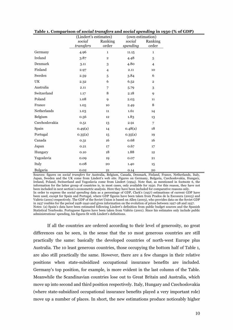
Table 1 shows a comparison between the levels of social transfers estimated by

Lindert for 1930 and my estimations of social spending for the same year. As expected,

the levels of social spending are higher in my estimation, which includes state-

subsidized occupational insurance benefits. Only in the cases of Finland and

Yugoslavia, Lindert's figures are slightly higher than those presented here, which is

probably explained by the fact that the sources used are not exactly the same. In some

countries the difference between the two estimates is not very wide. For instance, my

estimate for Ireland amounts to 4.48% of GDP as opposed to 3.87% in the case of

Lindert’s data. However, sometimes the difference is much bigger. For example, social

spending in the UK in 1930 was 6.52% of GDP, according to my estimations, while

according to Lindert's estimations it was just 2.32%. In the case of Czechoslovakia, my

estimations of social spending are also much higher: 2.91% of GDP as opposed to

0.51%.

specific legislation for each type of risk. The provisions of pure private insurance have not been included in the estimations. 11 The countries in the sample are: Australia, Austria, Belgium, Brazil, Bulgaria, Canada, Czechoslovakia, Denmark, Finland, France, Germany, Greece, the Netherlands, New Zealand, Norway, Hungary, Ireland, Italy, Japan, Poland, Portugal, the Soviet Union, Spain, Sweden, Switzerland, the United Kingdom, the United States and Yugoslavia. In some cases, the information for certain social spending items were not available for 1930 and 1933 but for other nearby years such as 1929, 1931 or 1934. 12 Table A.1 in the appendix shows my new estimates of social spending.

10

Table 1. Comparison of social transfers and social spending in 1930 (% of GDP)

(Lindert’s estimates) (own estimation)

social transfers

Ranking order

social spending

Ranking order

Germany 4.96 1 11.15 1

Ireland 3.87 2 4.48 5

Denmark 3.11 3 4.80 4

Finland 2.97 4 2.11 10

Sweden 2.59 5 3.84 6

UK 2.32 6 6.52 2

Australia 2.11 7 5.79 3

Switzerland 1.17 8 2.18 9

Poland 1.08 9 2.03 11

France 1.05 10 2.49 8

Netherlands 1.03 11 1.61 14

Belgium 0.56 12 1.83 13

Czechoslovakia 0.51 13 2.91 7

Spain 0.49(a) 14 0.48(a) 18

Portugal 0.35(a) 15 0.35(a) 19

Canada 0.31 16 0.68 16

Japan 0.21 17 0.67 17

Hungary 0.10 18 1.88 12

Yugoslavia 0.09 19 0.07 21

Italy 0.08 20 1.40 15

Bulgaria 0.02 21 0.14 20 Sources: figures on social transfers for Australia, Belgium, Canada, Denmark, Finland, France, Netherlands, Italy, Japan, Sweden and the UK come from Lindert’s web site. Figures on Germany, Bulgaria, Czechoslovakia, Hungary, Ireland, Poland, Switzerland and Yugoslavia come from Lindert (1994). Note that, as mentioned in footnote 6, the information for the latter group of countries is, in most cases, only available for 1930. For this reason, they have not been included in next section’s econometric analysis. Here they have been included for comparative reasons only. In order to express the social spending data as a percentage of GDP, Clark's (1957) estimations of current GDP have been used, except for Spain and Portugal, where GDP figures have been taken from Prados de la Escosura (2003) and Valério (2001) respectively. The GDP of the Soviet Union is based on Allen (2003), who provides data on the Soviet GDP in 1937 roubles for the period 1928-1940 and gives information on the evolution of prices between 1927-28 and 1937. Notes: (a) Spain’s data have been estimated following Lindert’s definition from public budget sources and the Spanish Statistical Yearbooks. Portuguese figures have been taken from Valério (2001). Since his estimates only include public administrations’ spending, his figures fit with Lindert’s definitions.

If all the countries are ordered according to their level of generosity, no great

differences can be seen, in the sense that the 10 most generous countries are still

practically the same: basically the developed countries of north-west Europe plus

Australia. The 10 least generous countries, those occupying the bottom half of Table 1,

are also still practically the same. However, there are a few changes in their relative

positions when state-subsidized occupational insurance benefits are included.

Germany's top position, for example, is more evident in the last column of the Table.

Meanwhile the Scandinavian countries lose out to Great Britain and Australia, which

move up into second and third position respectively. Italy, Hungary and Czechoslovakia

(where state-subsidized occupational insurance benefits played a very important role)

move up a number of places. In short, the new estimations produce noticeably higher

11

figures for social spending than Lindert's estimations and also bring about changes in

relative positions, with a relative improvement of those countries where state-

subsidized occupational insurance played an important role.

Finally, as in the case of Lindert’s data, my estimates can also be broken down

by programme. However, the information contained in the ILO reports is not

completely homogeneous. Classification criteria and the level of detail of the

information varied from country to country. Despite the difficulties, I have been able to

classify benefits into 3 categories of social spending: pensions, health, and welfare and

unemployment. The first one includes old-age, survivor’s and widow's pensions, plus

workmen’s compensation. The second awarded disability pensions and also temporary

incapacity benefits. However, it was impossible to distinguish between them.

Consequently they have all been grouped together under the pensions heading. Health

spending includes health-care spending plus sickness and maternity leave benefits.

Finally, spending on welfare and unemployment includes family allowances, benefits

for the unemployed, and the traditional poor-relief which was often given to the sick,

the unemployed or the elderly without distinguishing between them.

3. The determinants of social transfers between 1880 and 1930

The aim of this section is to analyse the role of inequality in the early stages of

social policy. The basic model to be estimated is given by Equation (1):

(1) 1210

εααα +++= ZINEQREDIST

where REDIST is the level of redistribution, INEQ is the level of inequality, and

Z is a group of variables that are normally included in comparative studies on the

determinants of social policy. The series of social transfers estimated by Lindert is used,

in this section, as an indicator of redistribution. As mentioned earlier, it covers the

time-period 1880-1930; the information is available for 10-year intervals (1880, 1890,

1900, 1910, 1920 and 1930) and embraces 21 different countries. In the case of Spain

the figures are my own and in the case of Portugal they come from Valério (2001).

Three alternative variables that capture the distribution of income have been

used as a proxy of inequality: the top income shares, the ratio of the GDP per capita to

the unskilled wage, and the area of non-family farms as a percentage of the total farm

12

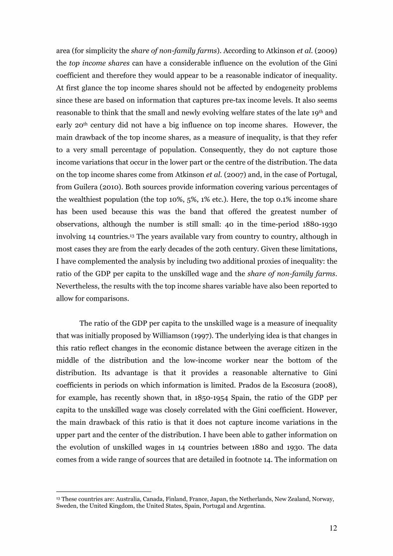
area (for simplicity the share of non-family farms). According to Atkinson et al. (2009)

the top income shares can have a considerable influence on the evolution of the Gini

coefficient and therefore they would appear to be a reasonable indicator of inequality.

At first glance the top income shares should not be affected by endogeneity problems

since these are based on information that captures pre-tax income levels. It also seems

reasonable to think that the small and newly evolving welfare states of the late 19th and

early 20th century did not have a big influence on top income shares. However, the

main drawback of the top income shares, as a measure of inequality, is that they refer

to a very small percentage of population. Consequently, they do not capture those

income variations that occur in the lower part or the centre of the distribution. The data

on the top income shares come from Atkinson et al. (2007) and, in the case of Portugal,

from Guilera (2010). Both sources provide information covering various percentages of

the wealthiest population (the top 10%, 5%, 1% etc.). Here, the top 0.1% income share

has been used because this was the band that offered the greatest number of

observations, although the number is still small: 40 in the time-period 1880-1930

involving 14 countries.13 The years available vary from country to country, although in

most cases they are from the early decades of the 20th century. Given these limitations,

I have complemented the analysis by including two additional proxies of inequality: the

ratio of the GDP per capita to the unskilled wage and the share of non-family farms.

Nevertheless, the results with the top income shares variable have also been reported to

allow for comparisons.

The ratio of the GDP per capita to the unskilled wage is a measure of inequality

that was initially proposed by Williamson (1997). The underlying idea is that changes in

this ratio reflect changes in the economic distance between the average citizen in the

middle of the distribution and the low-income worker near the bottom of the

distribution. Its advantage is that it provides a reasonable alternative to Gini

coefficients in periods on which information is limited. Prados de la Escosura (2008),

for example, has recently shown that, in 1850-1954 Spain, the ratio of the GDP per

capita to the unskilled wage was closely correlated with the Gini coefficient. However,

the main drawback of this ratio is that it does not capture income variations in the

upper part and the center of the distribution. I have been able to gather information on

the evolution of unskilled wages in 14 countries between 1880 and 1930. The data

comes from a wide range of sources that are detailed in footnote 14. The information on

13 These countries are: Australia, Canada, Finland, France, Japan, the Netherlands, New Zealand, Norway, Sweden, the United Kingdom, the United States, Spain, Portugal and Argentina.

13

the GDP per capita has been taken from Maddison.14 Given my model, one possible

concern regarding the ratio of the GDP per capita to the unskilled wage is that this

variable might be affected by endogeneity problems, because the unskilled wage might

be affected by social programs. As is shown below, I have applied some endogeneity

tests and there is no evidence suggesting that this indicator is significantly affected by

endogeneity problems. Perhaps, this is because the social programs implemented in

1880-1933 were not big enough to affect market inequality in a significant way.

Lastly, I have also used the share of non-family farms as a proxy of inequality.

The information has been taken from Vanhanen (1997), who defines a family farm as

one that provides work for a maximum of four people, including family members. The

size of family farms can therefore change over time and from one country to another,

depending on the technology or weather conditions. The purpose of this criterion is to

separate family farms from big farms worked by paid employees. Note that it is the

share of non-family farms (the opposite of Vanhanen's share of family farms) that is

used here, because the aim is to have an indicator of inequality, not equality.

Apparently, the share of non-family farms variable has the advantage of not being

subject to problems of reverse causality, because there is no reason to think that social

transfers had a direct influence on the distribution of land ownership. However, this

indicator loses representativity as the industrialization process advances and

agriculture loses weight in the economy. Even so, it appears to be a reasonable proxy,

especially in a period such as the one analyzed here on which information is very

limited and the agrarian sector was much more important than nowadays. In fact, this

variable has been used in a number of earlier studies as a proxy for overall inequality

(Vanhanen, 1997; Boix, 2003; Keefer and Knack, 2002; Alesina and Rodrik, 1994).

Here, I have decided to keep this variable to make the exercise more robust and to

14 For Belgium, France, Italy, the Netherlands and the UK, the wage information between 1880 and 1910 has been taken from Allen (2001), while in 1920 and 1930 it comes from Scholliers (1995), Sicsic (1995), Scholliers and Zamagni (1995), Vermaas (1995) and Feinstein (1995), respectively. Wages in 1920 and 1930 have been rescaled to make them equal to those from Allen (2001) in 1910. Wage data for Canada, Denmark, Norway and the United States comes from the historical statistics of the respective country. For Sweden, wage information comes from Björklund and Stenlund (1995). In the case of Spain, the information in 1880-1900 comes from Reher and Ballesteros (1995), while in 1910-30 it comes from Vilar (2005). In the case of Portugal, the data has been taken from Martins (1997), and for Australia and New Zealand it comes from ILO (1938) and Mitchell (2003). Information on New Zealand for 1880-1910, Australia for 1880-1900, and Portugal for 1920-30 is missing. Therefore the total number of available observations is 75. Most of my wage data refers to unskilled labor in the construction sector. On the other hand, between 1880 and 1930 there was a considerable variation in working hours. Therefore, to make the international comparison more informative, I have computed the annual disposable income of unskilled workers. To make the calculations working-hours data has been taken from Huberman and Minns (2007). Next, nominal wages have been deflated by using Maddison (1991)’s price index (this should help to keep consistency with Maddison’s GDP figures). And national real wages have been transformed to US dollars to calculate international real wage indices for which the real wage in the US for 1910 has been set equal to 100. Maddison’s GDP figures have also been indexed by setting US real GDP per capita in 1910 equal to 100.

14

allow comparisons with the results obtained with the top income shares and the ratio of

the GDP per capita to the unskilled wage. Moreover, this is the proxy for which I have

more observations available. However, one needs to keep in mind the limitations of this

variable when interpreting the results.

The control variables (parameter Z in Equation 1) include the logarithm of GDP

per capita, the ageing of population –measured by the percentage of population over

65– and the degree of political democratization. GDP figures come from Maddison, and

the percentage of population over 65 has been taken from the Lindert website database,

except for Spain, which comes from Nicolau (2005). The expected sign of the

coefficients of both the income level and the ageing of population variables is positive.

Pampel and Williamson (1989) and Mulligan et al. (2010), in fact, consider that these

are the most important variables to explain the development of social policy. The

degree of democratization, meanwhile, has been measured as the extension of voting

rights –calculated as the number of registered voters as a percentage of the population

over 20 years old-.15 Since voting rights only are effective when certain conditions of

political freedom and political party competition are fulfilled, when the autocracy

index of the Polity IV Project was higher than the democracy index, I have set my

democracy variable equal to zero (that is, I have assumed that the situation was similar

to that in which there were no voting rights –one example in my sample is Portugal in

1880-1900).16

The expected sign of the degree of democratization, however, is less clear than

in the case of the level of GDP per capita and the ageing of population. Initially one

might think that democracy should have a positive effect on social spending, since it

guarantees the right to vote to lower-income groups and allows the existence of left-

wing parties and workers' unions (Lindert, 1994; Hicks, 1999; Espuelas, 2012).

Mulligan et al. (2010), however, maintain that social spending is mostly driven by

economic and demographic factors and that democracy is not a key determinant of the

development of social policy. Hence the expected sign of this variable is not clear.

15 Data on registered voters has been taken from the Bank’s cross-national time-series database, completed with Mackie and Rose (1991). When calculating my index of the extension of voting rights for countries and time-periods in which voting rights were limited to the male population, I have used the male population over 20 years old as the denominator. When voting rights were extended to women, then I have used the whole population over 20 years old. 16 I have also estimated the model: 1) taking the number of registered voters as a percentage of the population over 20 years old, and 2) including a dummy variable to control for the existence of democracy, and the results are very similar.

15

Results

The results of estimating the basic model given in equation (1), using my three

alternative proxies of inequality, are shown in Table 2. The estimation method used in

the regressions is least squares with country random-effects. Particularly in the

regressions in which the top income shares are used as a proxy of inequality the

random-effects model is preferred to the fixed-effects model. Given the scant number

of observations, the latter would have been very costly in terms of losing degrees of

freedom. The Hausman test was applied and no evidence was found to reject the

random-effects model. Following Niskanen (1971), one might argue that once social

programmes are established they have a tendency to grow by themselves (due to the

aspirations of bureaucracy), giving rise to a kind of inertia effect. In other words, the

growth of social transfers may be no more than the result of a simple time trend.

Similarly, one might argue that the evolution of social transfers depends on shocks

occurring at specific moments, such as the impact of the World War I or the copycat

effect that may have come about after the pioneering countries introduced the first

social protection measures. To test both possibilities and give more robustness to the

analysis, I have also estimated the model including a time trend (that should capture

the inertia effect) and time fixed-effects (that should capture the influence of specific

shocks). Finally, as in Lindert (1994), the results of estimating a tobit model are also

reported (columns 10 and 11), because the endogenous variable, the level of social

transfers as a share of GDP, is partially censored. Particularly at the beginning of the

time-period, there are several observations taking value zero.17

17 The results of the tobit model with the top income shares variable are not reported because there is only one single censored observation.

16

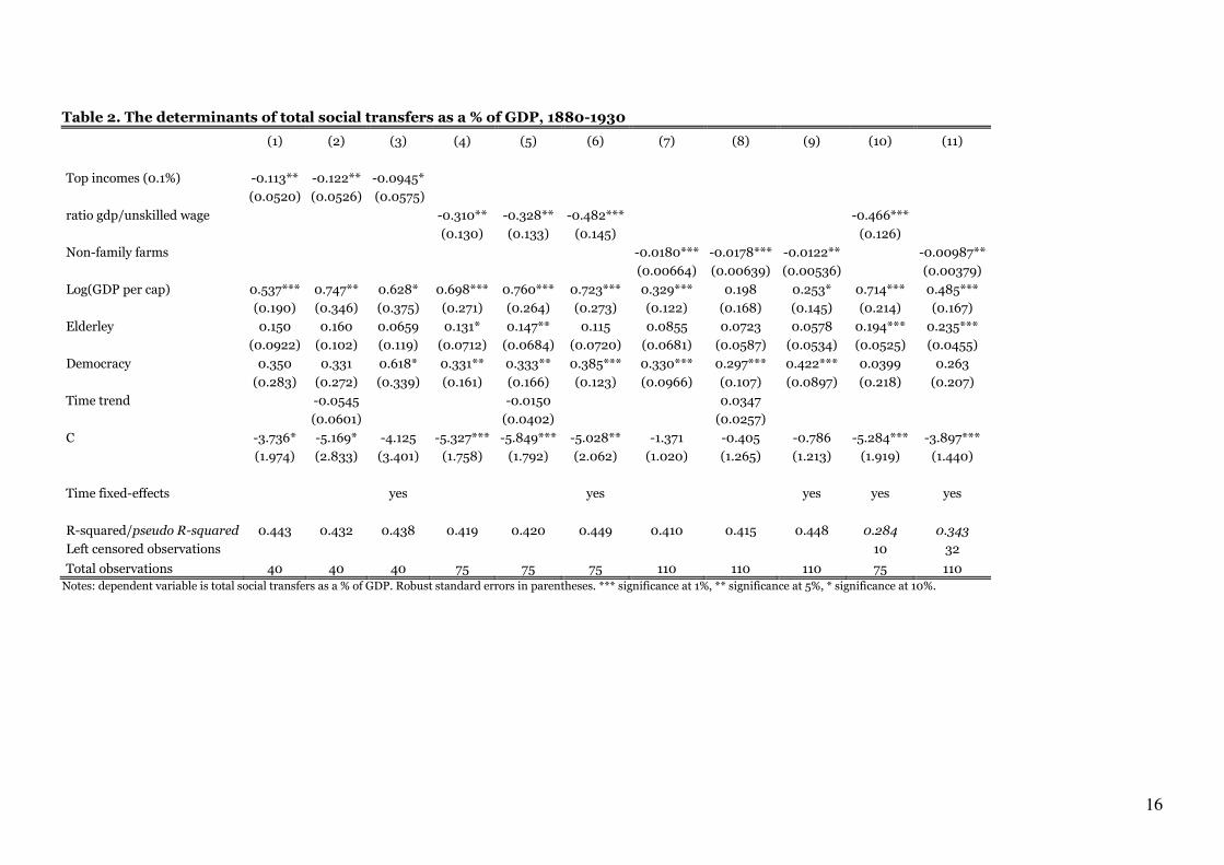
Table 2. The determinants of total social transfers as a % of GDP, 1880-1930

(1) (2) (3) (4) (5) (6) (7) (8) (9) (10) (11)

Top incomes (0.1%) -0.113** -0.122** -0.0945*

(0.0520) (0.0526) (0.0575)

ratio gdp/unskilled wage

-0.310** -0.328** -0.482***

-0.466***

(0.130) (0.133) (0.145)

(0.126)

Non-family farms

-0.0180*** -0.0178*** -0.0122**

-0.00987**

(0.00664) (0.00639) (0.00536)

(0.00379)

Log(GDP per cap) 0.537*** 0.747** 0.628* 0.698*** 0.760*** 0.723*** 0.329*** 0.198 0.253* 0.714*** 0.485***

(0.190) (0.346) (0.375) (0.271) (0.264) (0.273) (0.122) (0.168) (0.145) (0.214) (0.167)

Elderley 0.150 0.160 0.0659 0.131* 0.147** 0.115 0.0855 0.0723 0.0578 0.194*** 0.235***

(0.0922) (0.102) (0.119) (0.0712) (0.0684) (0.0720) (0.0681) (0.0587) (0.0534) (0.0525) (0.0455)

Democracy 0.350 0.331 0.618* 0.331** 0.333** 0.385*** 0.330*** 0.297*** 0.422*** 0.0399 0.263

(0.283) (0.272) (0.339) (0.161) (0.166) (0.123) (0.0966) (0.107) (0.0897) (0.218) (0.207)

Time trend

-0.0545

-0.0150

0.0347

(0.0601)

(0.0402)

(0.0257)

C -3.736* -5.169* -4.125 -5.327*** -5.849*** -5.028** -1.371 -0.405 -0.786 -5.284*** -3.897***

(1.974) (2.833) (3.401) (1.758) (1.792) (2.062) (1.020) (1.265) (1.213) (1.919) (1.440)

Time fixed-effects

yes

yes

yes yes yes

R-squared/pseudo R-squared 0.443 0.432 0.438 0.419 0.420 0.449 0.410 0.415 0.448 0.284 0.343

Left censored observations

10 32

Total observations 40 40 40 75 75 75 110 110 110 75 110

Notes: dependent variable is total social transfers as a % of GDP. Robust standard errors in parentheses. *** significance at 1%, ** significance at 5%, * significance at 10%.

17

As expected, the level of GDP per capita shows a positive impact on total social

transfers. The coefficient of the ageing of population is also positive but it is only

significant in 4 out of 12 regressions. As for the coefficient associated to the degree of

democratization, it is also positive and significant in most of the regressions. This

suggests that the advent of democracy and the subsequent incorporation of low-income

groups into the political process stimulated the development of social policy.

Inequality, on the other hand, has a negative and significant effect, no matter whether

it is approximated by the top income shares, the ratio of the GDP to the unskilled wage

or the share of non-family farms. This is just the opposite of what would have been

expected according to the median voter models. Moreover, the results hold when

controlling for time fixed-effects and a time-trend, suggesting that the observed

negative correlation is not the result of the passage of time or an inertia effect.

However, the main potential concern is that the results in table 2 might be biased

because of the existence of endogeneity. On the one hand, both the top income shares

and the ratio of the GDP to the unskilled wage might be influenced by (past) social

transfers, which would lead to inverse causality and endogeneity problems. On the

other hand, the share of non-family farms is less likely to be affected by current or past

social transfers. However, its evolution is unlikely to be random. On the contrary, one

might argue that the share of non-family farms is likely to diminish over time (because

of the introduction of new technology, for example, allowing families to work bigger

extensions of land without hiring employees).

To test for the existence of endogeneity, I have implemented the Durbin-Wu-

Hausman (DWH) specification test. The models tested are the specifications given in

columns 3, 6 and 9 of Table 2. In the instrumental variable estimates, I have used the

lagged values of social transfers and inequality as the instruments for inequality. The

results of the DWH test are the following. In the case of the specification with the top

income shares as a proxy of inequality the statistic associated to the DWH test is chi-

squared (1) = 1.59, which indicates that there is weak evidence against the null that the

regressor is exogenous. This result, however, should be interpreted with caution

because of the scant number of observations. In the case of the ratio of the GDP per

capita to the unskilled wage, the statistic associated to the DWH test is chi-squared (1)

= 0.21. Again, no evidence is found to reject the least squares model. As suggested

before, these results seem to indicate that social programs of the late 19th and early 20th

centuries were not big enough to affect market inequality in a significant way.

18

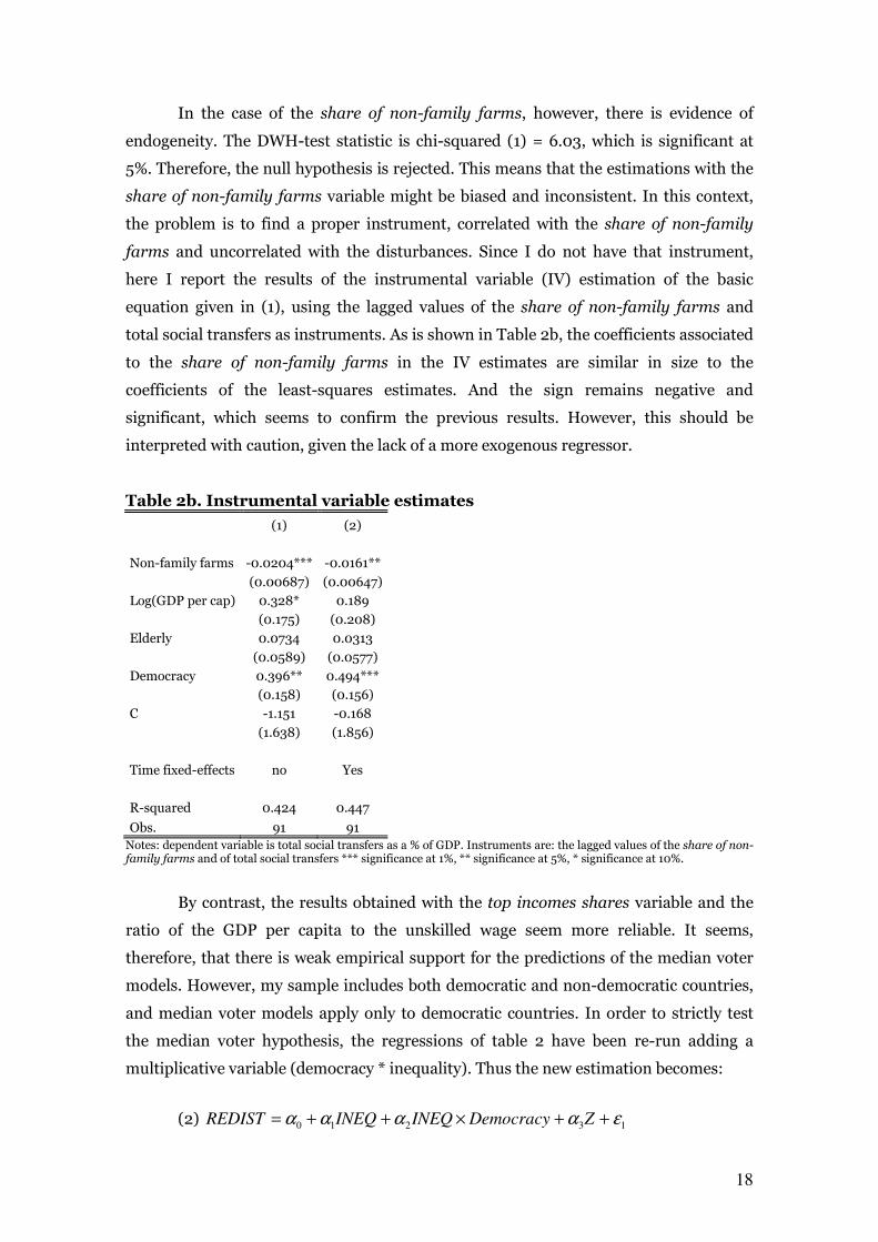
In the case of the share of non-family farms, however, there is evidence of

endogeneity. The DWH-test statistic is chi-squared (1) = 6.03, which is significant at

5%. Therefore, the null hypothesis is rejected. This means that the estimations with the

share of non-family farms variable might be biased and inconsistent. In this context,

the problem is to find a proper instrument, correlated with the share of non-family

farms and uncorrelated with the disturbances. Since I do not have that instrument,

here I report the results of the instrumental variable (IV) estimation of the basic

equation given in (1), using the lagged values of the share of non-family farms and

total social transfers as instruments. As is shown in Table 2b, the coefficients associated

to the share of non-family farms in the IV estimates are similar in size to the

coefficients of the least-squares estimates. And the sign remains negative and

significant, which seems to confirm the previous results. However, this should be

interpreted with caution, given the lack of a more exogenous regressor.

Table 2b. Instrumental variable estimates

(1) (2)

Non-family farms -0.0204*** -0.0161**

(0.00687) (0.00647)

Log(GDP per cap) 0.328* 0.189

(0.175) (0.208)

Elderly 0.0734 0.0313

(0.0589) (0.0577)

Democracy 0.396** 0.494***

(0.158) (0.156)

C -1.151 -0.168

(1.638) (1.856)

Time fixed-effects no Yes

R-squared 0.424 0.447

Obs. 91 91

Notes: dependent variable is total social transfers as a % of GDP. Instruments are: the lagged values of the share of non-family farms and of total social transfers *** significance at 1%, ** significance at 5%, * significance at 10%.

By contrast, the results obtained with the top incomes shares variable and the

ratio of the GDP per capita to the unskilled wage seem more reliable. It seems,

therefore, that there is weak empirical support for the predictions of the median voter

models. However, my sample includes both democratic and non-democratic countries,

and median voter models apply only to democratic countries. In order to strictly test

the median voter hypothesis, the regressions of table 2 have been re-run adding a

multiplicative variable (democracy * inequality). Thus the new estimation becomes:

(2) 13210

εαααα ++×++= ZDemocracyINEQINEQREDIST

19

where DemocracyINEQ× is the new multiplicative variable and the rest of the

parameters are the same as in Equation (1). The total marginal effect of inequality

under democracy in this new estimation would be:

(3) DemocracyINEQREDIST ×+=∂∂21

/ αα

Notice that my democracy indicator is a continuous variable that ranges

between 0 and 1 (where 1 means that the whole adult population is enfranchised), and

that my inequality proxies grow with inequality. Therefore, if the predictions of the

median voter models are correct, the new multiplicative variable should have a positive

sign: the greater the inequality and the more democratic the political context, the

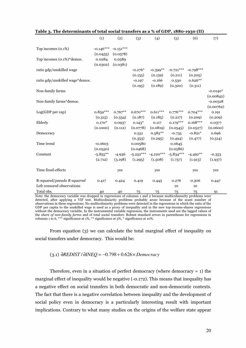
greater the level of redistribution should be. However, the results of the econometric

regressions do not seem to confirm this hypothesis. As is shown in Table 3, the

coefficient associated with the multiplicative variable is not significant in most of the

regressions. This suggests that the impact of inequality, even in democracy, continues

to be negative. The only exception is the regression of column 7 in which the interaction

between democracy and inequality has appositive sign and is statistically significant.

The coefficient, however, is too small to compensate for the negative effect of

inequality.

20

Table 3. The determinants of total social transfers as a % of GDP, 1880-1930 (II)

(1) (2) (3) (4) (5) (6) (7)

Top incomes (0.1%) -0.146*** -0.151***

(0.0455) (0.0578)

Top incomes (0.1%)*democ. 0.0284 0.0589

(0.0302) (0.0381)

ratio gdp/unskilled wage

-0.276* -0.399** -0.721*** -0.798***

(0.155) (0.159) (0.211) (0.205)

ratio gdp/unskilled wage*democ.

-0.197 -0.166 0.530 0.626**

(0.195) (0.189) (0.320) (0.311)

Non-family farms

-0.0140*

(0.00842)

Non-family farms*democ.

-0.00318

(0.00762)

Log(GDP per cap) 0.859*** 0.767** 0.670*** 0.611*** 0.776*** 0.704*** 0.191

(0.315) (0.334) (0.187) (0.185) (0.217) (0.209) (0.209)

Elderly 0.170* 0.0937 0.143* 0.117 0.179*** 0.168*** 0.0377

(0.1000) (0.112) (0.0778) (0.0819) (0.0545) (0.0527) (0.0600)

Democracy

0.551 0.582** -0.735 -0.821* 0.696

(0.353) (0.295) (0.494) (0.477) (0.514)

Time trend -0.0603

0.00580

0.0645

(0.0550)

(0.0468)

(0.0586)

Constant -5.855** -4.936 -5.252*** -4.220*** -5.834*** -4.492** -0.353

(2.712) (3.198) (1.295) (1.508) (1.757) (1.913) (1.937)

Time fixed-effects

yes

yes

yes yes

R-squared/pseudo R-squared 0.417 0.424 0.419 0.445 0.276 0.306 0.447

Left censored observations

10 10 Total obs. 40 40 75 75 75 75 91

Note: the democracy variable was dropped in regressions of columns 1 and 2 because multicolinearity problems were detected, after applying a VIF test. Multicoliniarity problems probably arose because of the scant number of observations in these regressions. No multicoliniarity problems were detected in the regressions in which the ratio of the GDP per capita to the unskilled wage is used as a proxy of inequality and in the new top-income-shares regressions without the democracy variable. In the instrumental variable regression, the instruments used are the lagged values of the share of non-family farms and of total social transfers. Robust standard errors in parentheses for regressions in columns 1 to 6, *** significance at 1%, ** significance at 5%, * significance at 10%.

From equation (3) we can calculate the total marginal effect of inequality on

social transfers under democracy. This would be:

(3.1) DemocracyINEQREDIST ×+−=∂∂ 626.0798.0/

Therefore, even in a situation of perfect democracy (where democracy = 1) the

marginal effect of inequality would be negative (-0.172). This means that inequality has

a negative effect on social transfers in both democratic and non-democratic contexts.

The fact that there is a negative correlation between inequality and the development of

social policy even in democracy is a particularly interesting result with important

implications. Contrary to what many studies on the origins of the welfare state appear

21

to implicitly suggest, inequality did not favour the development of social policy even in

its initial stages (when the level of social transfers was really low and social needs were

therefore greater than today). However, the fact that social spending is negatively

correlated with inequality suggests that unequal societies were in a sort of inequality

trap, in the sense that inequality itself was an obstacle to redistribution.

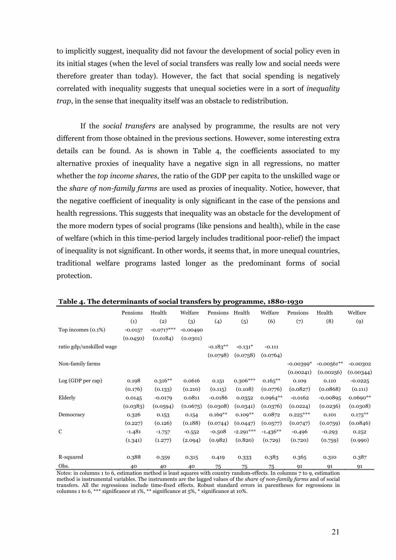
If the social transfers are analysed by programme, the results are not very

different from those obtained in the previous sections. However, some interesting extra

details can be found. As is shown in Table 4, the coefficients associated to my

alternative proxies of inequality have a negative sign in all regressions, no matter

whether the top income shares, the ratio of the GDP per capita to the unskilled wage or

the share of non-family farms are used as proxies of inequality. Notice, however, that

the negative coefficient of inequality is only significant in the case of the pensions and

health regressions. This suggests that inequality was an obstacle for the development of

the more modern types of social programs (like pensions and health), while in the case

of welfare (which in this time-period largely includes traditional poor-relief) the impact

of inequality is not significant. In other words, it seems that, in more unequal countries,

traditional welfare programs lasted longer as the predominant forms of social

protection.

Table 4. The determinants of social transfers by programme, 1880-1930

Pensions Health Welfare Pensions Health Welfare Pensions Health Welfare

(1) (2) (3) (4) (5) (6) (7) (8) (9)

Top incomes (0.1%) -0.0157 -0.0717*** -0.00490

(0.0450) (0.0184) (0.0301)

ratio gdp/unskilled wage

-0.183** -0.131* -0.111

(0.0798) (0.0758) (0.0764)

Non-family farms

-0.00399* -0.00561** -0.00302

(0.00241) (0.00256) (0.00344)

Log (GDP per cap) 0.198 0.316** 0.0616 0.151 0.306*** 0.165** 0.109 0.110 -0.0225

(0.176) (0.133) (0.210) (0.115) (0.108) (0.0776) (0.0827) (0.0868) (0.111)

Elderly 0.0145 -0.0179 0.0811 -0.0186 0.0352 0.0964** -0.0162 -0.00895 0.0690**

(0.0383) (0.0594) (0.0675) (0.0308) (0.0341) (0.0376) (0.0224) (0.0236) (0.0308)

Democracy 0.326 0.153 0.154 0.169** 0.109** 0.0872 0.225*** 0.101 0.175**

(0.227) (0.126) (0.188) (0.0744) (0.0447) (0.0577) (0.0747) (0.0759) (0.0846)

C -1.481 -1.757 -0.552 -0.508 -2.291*** -1.436** -0.496 -0.293 0.252

(1.341) (1.277) (2.094) (0.982) (0.820) (0.729) (0.720) (0.759) (0.990)

R-squared 0.388 0.359 0.315 0.419 0.333 0.383 0.365 0.310 0.387

Obs. 40 40 40 75 75 75 91 91 91

Notes: in columns 1 to 6, estimation method is least squares with country random-effects. In columns 7 to 9, estimation method is instrumental variables. The instruments are the lagged values of the share of non-family farms and of social transfers. All the regressions include time-fixed effects. Robust standard errors in parentheses for regressions in columns 1 to 6, *** significance at 1%, ** significance at 5%, * significance at 10%.

22

4. The determinants of social spending in 1930-33

As was seen earlier, in many countries the rise of the welfare state was closely

linked to the development of state-subsidized occupational insurance programs. The

aim of this section is to analyse whether the negative effect of inequality is maintained

when the provisions of these programs are included in the analysis. Therefore, the new

estimation of social spending presented in Section 3 has been used as the endogenous

variable for the analysis. As before, I have used the top income shares, the ratio of the

GDP per capita to the unskilled wage and the share of non-family farms18 as proxies of

inequality. The estimation method is least squares and, given the low number of

observations, it was considered best to include random effects instead of fixed effects

since the latter would be very costly in terms of losing degrees of freedom. Also, some

explanatory variables take the same value in 1930 as in 1933 because the information is

only available for every 10 years or covers various years, and they therefore act as a

quasi fixed-effect. As before, in the case of the regressions with the share of non-family

farms, the estimation method is instrumental variables, using the share of non-family

farms in 1920 as an instrument.

The rest of the explanatory variables are practically the same as in the previous

section. The percentage of population over 65 has been used to capture the effect of the

ageing of population. The data come from Lindert's website, except in the case of

Bulgaria, Czechoslovakia, Hungary, Ireland, Poland, the Soviet Union and Yugoslavia,

for which they have been taken from Mitchell (1998). The percentage of registered

voters over the adult population has again been used to measure the degree of

democratization. In order to avoid possible distortions brought about by the impact of

the Great Depression, instead of GDP per capita I have included the percentage of the

working population in agriculture, which is a more stable indicator of economic

development. The information comes from Mitchell (1998), except for the USSR and

Spain, for which it has been taken from Allen (2003) and Nicolau (2005) respectively.

Finally, in order to capture the effect of the economic cycle and, especially, to account

for the impact of the Great Depression, the rate of economic growth during the previous

five years (taken from Maddison) has also been included in the estimation.

18 In the Soviet Union the share of non-family farms takes value zero. In the 1930s, non-family farms basically belonged to the State and therefore they are not a good indicator of inequality or of the political influence of upper-income groups. In fact the political conditions in this country in the 1930s would make likely to assume that rural landowners had no political power and that the agrarian reform of 1917 and the subsequent collectivization brought about a radical decrease in inequality.

23

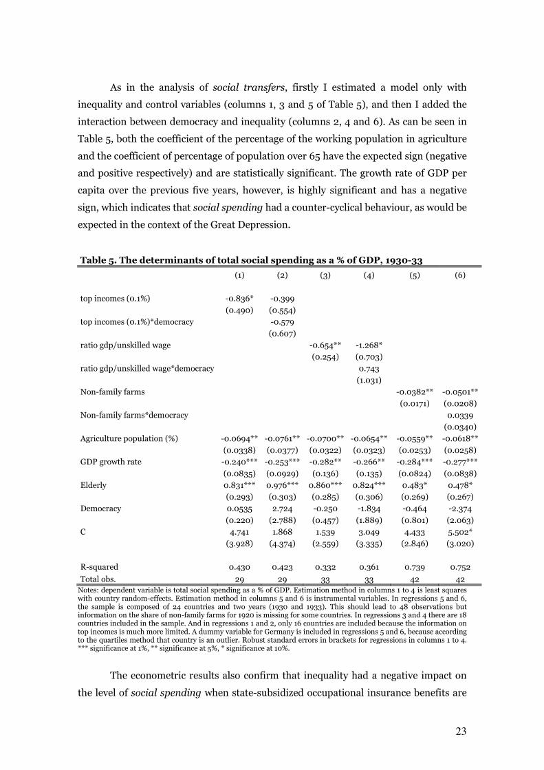
As in the analysis of social transfers, firstly I estimated a model only with

inequality and control variables (columns 1, 3 and 5 of Table 5), and then I added the

interaction between democracy and inequality (columns 2, 4 and 6). As can be seen in

Table 5, both the coefficient of the percentage of the working population in agriculture

and the coefficient of percentage of population over 65 have the expected sign (negative

and positive respectively) and are statistically significant. The growth rate of GDP per

capita over the previous five years, however, is highly significant and has a negative

sign, which indicates that social spending had a counter-cyclical behaviour, as would be

expected in the context of the Great Depression.

Table 5. The determinants of total social spending as a % of GDP, 1930-33

(1) (2) (3) (4) (5) (6)

top incomes (0.1%) -0.836* -0.399

(0.490) (0.554)

top incomes (0.1%)*democracy

-0.579

(0.607)

ratio gdp/unskilled wage

-0.654** -1.268*

(0.254) (0.703)

ratio gdp/unskilled wage*democracy

0.743

(1.031)

Non-family farms

-0.0382** -0.0501**

(0.0171) (0.0208)

Non-family farms*democracy

0.0339

(0.0340)

Agriculture population (%) -0.0694** -0.0761** -0.0700** -0.0654** -0.0559** -0.0618**

(0.0338) (0.0377) (0.0322) (0.0323) (0.0253) (0.0258)

GDP growth rate -0.240*** -0.253*** -0.282** -0.266** -0.284*** -0.277***

(0.0835) (0.0929) (0.136) (0.135) (0.0824) (0.0838)

Elderly 0.831*** 0.976*** 0.860*** 0.824*** 0.483* 0.478*

(0.293) (0.303) (0.285) (0.306) (0.269) (0.267)

Democracy 0.0535 2.724 -0.250 -1.834 -0.464 -2.374

(0.220) (2.788) (0.457) (1.889) (0.801) (2.063)

C 4.741 1.868 1.539 3.049 4.433 5.502*

(3.928) (4.374) (2.559) (3.335) (2.846) (3.020)

R-squared 0.430 0.423 0.332 0.361 0.739 0.752

Total obs. 29 29 33 33 42 42

Notes: dependent variable is total social spending as a % of GDP. Estimation method in columns 1 to 4 is least squares with country random-effects. Estimation method in columns 5 and 6 is instrumental variables. In regressions 5 and 6, the sample is composed of 24 countries and two years (1930 and 1933). This should lead to 48 observations but information on the share of non-family farms for 1920 is missing for some countries. In regressions 3 and 4 there are 18 countries included in the sample. And in regressions 1 and 2, only 16 countries are included because the information on top incomes is much more limited. A dummy variable for Germany is included in regressions 5 and 6, because according to the quartiles method that country is an outlier. Robust standard errors in brackets for regressions in columns 1 to 4. *** significance at 1%, ** significance at 5%, * significance at 10%.

The econometric results also confirm that inequality had a negative impact on

the level of social spending when state-subsidized occupational insurance benefits are

24

included in the analysis. Both the top income shares and the ratio of the GDP per capita

to the unskilled wage and the share of non-family farms have a negative sign and are

significant in almost all the regressions. The only exception is the regression in column

2, where the interaction between democracy and the top income shares is included.

However, neither the variable democracy nor the interaction between inequality and

democracy are significant in the regressions, which again suggests that even in

democracy there is a negative correlation between inequality and social spending.

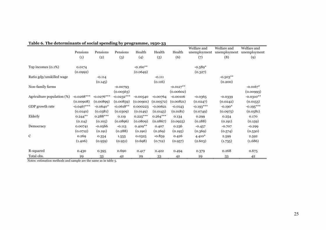
As in the previous section, I have also analysed the relationship between

inequality and social spending programme by programme. The results are shown in

Table 6. As expected, it seems that the percentage of the working population in

agriculture had a negative impact (although it is not significant in all regressions). The

ageing of population had a positive and significant effect on pensions and health; and

the GDP growth rate has a negative and significant sign, which again suggests that

social spending was counter-cycle. The coefficient associated to the variable democracy,

in contrast, is not statistically significant (it only shows a significant positive effect in

column 4). Finally, the coefficient associated to the inequality variables has a negative

sign in almost all regressions (the only exception is column 1). And it is statistically

significant in the regressions where health and welfare and unemployment are the

endogenous variables. Perhaps, this indicates that the response to increasing

unemployment during the 1930s was faster in more egalitarian countries. In any case, it

seems that inequality’s effect on social spending is also negative when specific social

programmes are analyzed. Therefore, again it seems that there is weak support for the

median voter hypothesis.

25

Table 6. The determinants of social spending by programme, 1930-33

Pensions Pensions Pensions Health Health Health Welfare and unemployment

Welfare and unemployment

Welfare and unemployment

(1) (2) (3) (4) (5) (6) (7) (8) (9)

Top incomes (0.1%) 0.0174

-0.160**

-0.589*

(0.0992)

(0.0649)

(0.327)

Ratio gdp/unskilled wage

-0.114

-0.111

-0.503**

(0.145)

(0.116)

(0.200)

Non-family farms

-0.00793

-0.0127**

-0.0167*

(0.00563)

(0.00602)

(0.00993)

Agriculture population (%) -0.0268*** -0.0276*** -0.0232*** -0.00540 -0.00764 -0.00106 -0.0365 -0.0339 -0.0310**

(0.00908) (0.00899) (0.00859) (0.00901) (0.00572) (0.00821) (0.0247) (0.0242) (0.0153)

GDP growth rate -0.0467*** -0.0640* -0.0618** 0.000223 -0.00621 -0.0143 -0.193*** -0.190* -0.195***

(0.0140) (0.0381) (0.0309) (0.0149) (0.0143) (0.0181) (0.0749) (0.0975) (0.0581)

Elderly 0.244** 0.288*** 0.119 0.225*** 0.264*** 0.134 0.299 0.254 0.170

(0.114) (0.105) (0.0896) (0.0809) (0.0867) (0.0925) (0.188) (0.191) (0.159)

Democracy 0.00741 -0.0566 -0.113 0.409** 0.407 0.236 -0.457 -0.707 -0.299

(0.0712) (0.191) (0.288) (0.190) (0.269) (0.195) (0.369) (0.574) (0.530)

C 0.269 0.354 1.555 0.0325 -0.859 0.426 4.410* 2.599 2.592

(1.406) (0.959) (0.951) (0.698) (0.712) (0.957) (2.603) (1.735) (1.686)

R-squared 0.430 0.395 0.690 0.417 0.422 0.494 0.379 0.268 0.675

Total obs. 29 33 42 29 33 42 29 33 42

Notes: estimation methods and sample are the same as in table 5.

26

In summary, the findings of these section and the previous one suggest that,

between 1880 and 1930-33, inequality had a rather negative influence on the

development of social policy, regardless of whether we use social transfers or social

spending as an indicator of redistribution, and regardless of whether we use the top

income shares, the ratio of the GDP per capita to the unskilled wage, or the share of

non-family farms as an indicator of inequality. This has some important implications

for economic growth. According to Alesina and Rodrik (1994) and Persson and

Tabellini (1994) inequality is harmful to economic growth because it leads to higher

redistribution and taxation. However, if my results are correct, these theories fail to

identify the mechanisms through which inequality hampers economic growth (because

inequality does not appear to result in higher redistribution, but the opposite). In fact,

there are a number of theories proposing alternative channels to explain why inequality

is bad for economic growth. Bénabou (1996), for example, considers that, if there are

market failures, inequality hampers human capital accumulation and, therefore,

economic growth. Perotti (1996), meanwhile, suggests that inequality stimulates

political violence, which, in turn, discourages investment. And Keefer and Knack

(2002) maintain that inequality increases political polarization, provoking uncertainty

on the protection of property rights and discouraging investment.

5. Conclusions

It is often assumed that the fight against inequality played an important role

during the early stages of the Welfare State. However, not many studies have tested this

hypothesis from a quantitative and comparative perspective. In this paper, the impact

of inequality on social policy between 1880 and 1930 has been analyzed, by using two

alternative indicators of redistribution -social transfers and social spending- and three

alternative proxies of inequality -the top income shares, the ratio of the GDP per capita

to the unskilled wage and the share of non-family farms-. Although it might look

counter-intuitive, the econometric outcomes show that inequality did not favour the

development of social policy even in its early stages. Curiously, more egalitarian

countries were also pioneers in the rise of the Welfare State. Somehow, this means that

unequal societies were in a sort of inequality trap, in the sense that inequality itself was

an obstacle to redistribution.

There are at least three theoretical arguments to explain this apparent paradox.

1) In the median voter theories it is assumed that redistribution implies dead-weight

27

losses. However, if there are market failures, as Bénabou (2000, 2005) stresses, then

redistribution can lead to efficiency gains, which (if inequality is low enough) can

compensate for the cost of redistribution. Instead, as inequality rises, so does the

number of individuals rich enough not to be compensated for the cost of redistribution.

Therefore, political support for redistribution will diminish. 2) In the median voter

theories it is also assumed that, in democracy, political power is equally distributed, as

all the citizens have the right to vote, and all the votes are worth the same. However,

according to a number of recent studies, power and political influence depend on

individuals’ income level. This means that if inequality increases then the political

power of the well-off will be also reinforced, so they will be able to stop redistribution

more easily. 3) Finally, it also looks plausible to consider, as Lindert (2004) does, that

political support for redistribution does not depend on the gap between the median

voter income and the average income, but on the gap between the median-income

groups (who are decisive in the elections) and the lower-income groups. The closer is

the distance between these two groups and the more the median-income groups believe

that they can become beneficiaries of social policy, the larger the political support for

redistribution.

Bibliography

Alesina, A. and Drazen, A., 1991. Why are stabilizations delayed. The American

Economic Review 81 (5), 1170-1188.

Alesina, A. and Rodrik, D., 1994. Distributive politics and economic growth. The

Quarterly Journal of Economics 109 (2), 465-490.

Alesina, A., Glaescer, E., and Sacerdote, B., 2001. Why doesn’t the United States

Have a European-Style Welfare State? Brooking Papers on Economic Activity 2, 187-

254.

Allen, R. C., 2001. The Great Divergence in European Wages and Prices from

the Middle Ages to the First World War. Explorations in Economic History 38, pp. 411-

447.

Allen, R. C., 2003. Farm to factory: a reinterpretation of the Soviet industrial

revolution. Princeton University Press, Princeton.

Ashford, D. E., 1989. La aparición de los Estados de Bienestar. Ministerio de

Trabajo y Seguridad Social, Madrid.

Atkinson, A. B., Piketty, T., and Saez, E., 2009. Top incomes in the long run of

history. NBER working paper 15408.

28

Atkinson, A. B. and Piketty, T. (Eds.), 2007. Top Incomes Over the Twentieth

Century. A Contrast Between Continental European and English-Speaking Countries.

Oxford University Press, Oxford.

Baldwin, P., 1990. The politics of Social Solidarity and the Bourgeois Basis of

the European Welfare State, 1875-1975. Cambridge University Press, Cambridge.

Bandrés, Eduardo (1999). Gasto Público y estructuras del bienestar: el sistema

de protección social. In: García Delgado, J. L. (dir.), España Economía: ante el siglo

XXI. Espasa Calpe, Madrid.

Bartels, L. M., 2002. Economic Inequality and Political Representation. Mimeo.

Barth, E. and Moene, K., 2009. The equality multiplier. NBER working paper

15076.

Bassett, W.F., Burkett, J.P. and Putterman, L., 1999. Income distribution,

government transfers, and the problem of unequal influence. European Journal of

Political Economy 15, 207-228.

Bénabou, R., 1996. Inequality and growth. NBER Macroeconomic Annual. MIT

Press, Cambridge, MA.

Bénabou, R., 2000. Unequal societies: income distribution and the social

contract. The American Economic Review 90 (1), 96-129.

Bénabou, R., 2005. Inequality, Technology and the Social Contract. In: Agion, P.

and Durlauf, S. N. (Eds.), Handbook f Economic Growth, Elsevier, Amsterdam, Oxford,

pp. 1596-1638.

Berg, A. and Sachs, J., 1988. The Debt Crisis: Structural Explanations of

Country Performance. Journal of Development Economics 29 (3), 271-306.

Björklund, J. and Stenlund, H., 1995. Real wages in Sweden, 1870-1950: a study

of six industrial branches. In: Scholliers, P. and Zamagni V. (eds.). Labour’s reward.

Edward Elgar, Aldershot Hants, pp. 151-166, 253-257.

Boix, C., 2003. Democracy and redistribution. Cambridge University Press,

Cambridge.

Clark, C., 1957. The conditions of Economic Progress. Macmillan, London.

Eitrheim, Ø., J.T. Klovland and J.F. Qvigstad (eds.), 2007. Historical Monetary

Statistics for Norway. Norges Bank, Oslo.

Elu, A., 2006. Las primeras pensiones públicas de vejez en España. Un estudio

del Retiro Obrero, 1909-1936. Revista de Historia Industrial 32 (3), 33-68.

Espuelas, S., 2012. Are dictatorships less redistributive? A comparative analysis

of social spending in Europe (1950-1980). European Review of Economic History 16

(2), 211-232.

29

Feinstein, Ch., 1995. Changes in nominal wages, the cost of living and real wages

in the United Kingdom over two centuries, 1780-1990. In: Scholliers, P. and Zamagni

V. (eds.). Labour’s reward. Edward Elgar, Aldershot Hants, pp. 3-36, 258-266.

Flora, P., 1983. State, economy and society in Western Europe, 1815-1975.

Campus Verlag, Frankfurt.

Flora, P. and Heidenheimer, A., (Eds.), 1981. The development of welfare state

in Europe and America. Transaction Books, New Brunswick (USA) and London (UK).

Fraser, D., [1973]2003. The Evolution of the British Welfare State. A History of

Social Policy since the Industrial Revolution. Palgrave Macmillan, Hampshire and New

York.

Guilera, J., 2010. The evolution of top income and wealth shares in Portugal

since 1936. Revista de Historia Económica, Journal of Iberian and Latin American

Economic History 28 (1), 139-171.

Herranz, A. (2010). La difusión internacional de los seguros sociales antes de

1945. In: Pons Pons J. and Silvestre Rodríguez J. (eds.), Los orígenes del Estado del

Bienestar en España, 1900-1945: los seguros de accidentes, vejez, desempleo y

enfermedad. Prensas universitarias de Zaragoza, Zaragoza.

Hicks, A., 1999. Social democracy and welfare capitalism. A century of income

security politics. Cornell University Press, London.

Huberman M. and Lewchuk, W., 2003. European economic integration and the

labour compact, 1850-1913. European Review of Economic History 7 (1), pp.3-41.

Huberman M. and Minns, C., 2007. The times are not changin’: Days and hours

of work in Old and New Worlds, 1870-2000. Explorations in Economic History 44,

pp.538-567.

International Labour Office, 1938. Year-book of labour statistics. ILO, Geneva.

Johansen, H. Ch., 1985. Dansk Økonomisk Statistik, 1814-1980. Gyldendal,

Copenhagen.

Keefer P. and Knack S., 2002. Polarization, politics and property rights: Links

between inequality and growth. Public Choice 111 (1-2), 127–154.

Kenworthy, L. and Pontusson, J., 2005. Rising Inequality and the Politics of

Redistribution in Affluent Countries. Perspectives on Politics 3 (3), 449-471.

Kristov, L., Lindert, P. H., and McClelland, R., 1992. Pressure groups and

redistribution. Journal of Public Economics 48 (2), 135-163.

Lindert, P.H., 1992. The Rise of Social Spending, 1880-1930. Working Paper

series, no. 68, Agricultural History Center, UC-Davis.

Lindert, P. H., 1994. The Rise of social Spending, 1880-1930. Explorations in

Economic History 31 (1), 1-37.

30

Lindert, P. H., 2004. Growing public social spending and economic growth

since the eighteenth century. Cambridge University Press, Cambridge.

Lynch, J., 2006. Age in the welfare state: the origins of social spending on

pensioners, workers, and children. Cambridge University Press, Cambridge.

Mackie, T. and Rose, R., 1991. The international almanac of electoral history.

Macmillan, London.

Maddison, A., 1991. Dynamic forces in capitalist development: a long run

comparative view. Oxford UP, New York.

Martins, C. A., 1997. Trabalho e condiçoes de vida em Portugal (1850-1913).

Análise Social, vol.XXXII (142), pp. 483-535.

Meltzer, A. H. and Richard, S. F., 1981. A rational theory of the size of

government. Journal of Political Economy 89 (5), 914-927.

Meltzer, A. H. and Richard, S. F., 1983. Tests of a rational theory of the size of

government. Public Choice 41 (3), 403-418.

Milanovic, B., 2000. The median-voter hypothesis, income inequality, and

income redistribution: an empirical test with the required data. European Journal of

Political Economy 16, 367-410.

Mitchell, B. R., 1998. International Historical Statistics: Europe, 1750-1993.

Stockton Press, Macmillan.

Mitchell, B. R., 2003. International Historical Statistics: Africa, Asia & Oceania

1750-2000. Palgrave Macmillan, New York.

Mulligan, C. B., Gil, R., and Sala-i-Martin, X., 2010. Social Security and

Democracy. The B.E. Journal of Economic Analysis and Policy 10 (1), article 18.

Murray, J. E., 2007. Origins of American health insurance: a history of

industrial sickness funds. Yale University Press, New Haven.

Nicolau, R., 2005. Población, salud, y actividad. In: Carreras, A. and Tafunell,

X. (coords.). Estadísticas históricas de España, vol. 1. Fundación BBVA, Bilbao, pp.

1027-1154.

Niskanen, W. A., 1971. Bureaucracy and Representative Government. Aldine,

Chicago.

OECD, 1985. Social expenditure: 1960-1990, Problems of growth and control.

OECD, Paris.

OECD, 2007. The social expenditure database: An interpretative guide. SOCX

1980-2003. OECD (www.oecd.org).

Pampel, F. C. and Williamson, J. B., 1989. Age, class, politics, and the welfare

state. Cambridge University Press, Cambridge.

31

Perotti, R., 1994. Income distribution and investment. European Economic

Review 38 (3-4), 827-835.

Perotti, R., 1996. Growth, Income Distribution, and Democracy: What the Data

Say. Journal of Economic Growth 1 (2), 149-187.

Persson, T. and Tabellini, G., 1994. Is inequality harmful for growth? American

Economic Review 84 (3), 600-621.

Prados de la Escosura, L., 2003. El progreso económico de España, 1850-2000.

Fundación BBVA, Bilbao.

Prados de la Escosura, L., 2008. Inequality, poverty and the Kuznets curve in

Spain, 1850-2000. European Review of Economic History 12, 287-324.

Reher, D. S. and Ballesteros, E. 1995. Precios y salaries en Castilla la Nueva: la

construcción de un índice de salarios reales, 1501-1991. Revista de historia económica

(11), pp. 101-151.

Rodrik, D., 1999. Where Did All the Growth Go? External Shocks, Social

Conflict, and Growth Collapses. Journal of Economic Growth 4 (4), 385-412.

Roemer, J. E., 1998. Why the poor do not expropriate the Rich: an old argument

in new garb. Journal of Public Economics, 70 (3), 399-424.

Rosenstone, S. and Hansen, J., 1993. Mobilization, Participation and

Democracy in America. MacMillan Publishing Company, New York.

Scholliers, P., 1995. A century of real wages in Belgium, 1840-1939. In:

Scholliers, P. and Zamagni V. (eds.). Labour’s reward. Edward Elgar, Aldershot Hants,

pp. 106-137, 203-205.

Scholliers, P. and Zamagni V. (eds.), 1995. Labour’s reward. Edward Elgar,

Aldershot Hants.

Sicsic, P., 1995. Wage dispersion in France, 1850-1930. In: Scholliers, P. and

Zamagni V. (eds.). Labour’s reward. Edward Elgar, Aldershot Hants, pp. 169-181, 206-

209.

Statistics Canada, 1983 [1999]. Historical Statistics of Canada

(http://www5.statcan.gc.ca/bsolc/olc-cel/olc-cel?catno=11-516-X&chropg=1&lang=eng)

Sutch, R. and Carter S. B., (eds.), 2006. The Historical Statistics of the United

States: Millennial Edition. Cambridge UP, New York.

Valério, N. (Ed.), 2001. Estatísticas Históricas Portuguesas. INE, Lisbon.

Vanhanen, T., 1997. Prospects of Democracy: a study of 172 countries.

Routledge, London and New York.

Vermaas, A., 1995. Real industrial wages in the Netherlands, 1850-1913. In:

Scholliers, P. and Zamagni V. (eds.). Labour’s reward. Edward Elgar, Aldershot Hants,

pp. 138-150, 234-237.

32

Vilar, M., 2005. Mercado de trabajo y crecimiento económico en España (1908-

1963): una nueva interpretación del primer franquismo. Mimeo.

Williamson, J. G., 1997. Globalization and Inequality, Past and Present. The

World Bank Research Observer 12 (2), 117-135.

Appendix

Table A.1. Social spending (as a % of GDP), 1930 and 1933

1930 1933

Australia 5.79 6.17

Austria 8.70

Belgium 1.83 5.85

Brazil 0.00

Bulgaria 0.14 0.17

Canada 0.68 2.15

Czechoslovakia 2.91 4.72

Denmark 4.8 6.32

Finland 2.11 2.57

France 2.49 3.97

Germany 11.15 12.41

Greece 0.50

Hungary 1.88 1.61

Ireland 4.48 5.44

Italy 1.4 1.4

Japan 0.67 0.51

Netherlands 1.61 6.56

New Zealand 5.45

Norway 4.72

Poland 2.03

Portugal 0.35 0.58

Spain 0.48 1.05

Sweden 3.84 6.02

Switzerland 2.18 3.54

United Kingdom 6.52 7.7

United States 3.21

URSS 1.81 2.55

Yugoslavia 0.07 0.14

Sources: see text.