The Indian Ocean Dipole: A Monopole in SST

YONGJING ZHAO AND SUMANT NIGAM

Department of Atmospheric and Oceanic Science, University of Maryland, College Park, College Park, Maryland

(Manuscript received 14 January 2014, in final form 13 May 2014)

ABSTRACT

The claim for a zonal-dipole structure in interannual variations of the tropical IndianOcean (IO) SSTs—the

Indian Ocean dipole (IOD)—is reexamined after accounting for El Niño–Southern Oscillation’s (ENSO)

influence. The authors seek an a priori accounting of ENSO’s seasonally stratified influence on IO SSTs and

evaluate the basis of the related dipole mode index, instead of seeking a posteriori adjustments to this index,

as common.

Scant observational evidence is found for zonal-dipole SST variations after removal of ENSO’s influence

from IOSSTs: The IODpoles are essentially uncorrelated in theENSO-filtered SSTs in both recent (1958–98)

and century-long (1900–2007) periods, leading to the breakdown of zonal-dipole structure in surface tem-

perature variability; this finding does not depend on the subtleties in estimation of ENSO’s influence.

Deconstruction of the fall 1994 and 1997 SST anomalies led to their reclassification, with a weak IOD in 1994

and none in 1997.

Regressions of the eastern IOD pole on upper-ocean heat content, however, do exhibit a zonal-dipole

structure but with the western pole in the central-equatorial IO, suggesting that internally generated basin

variability can have zonal-dipole structure at the subsurface.

The IO SST variability was analyzed using the extended-EOF technique, after removing the influence of

Pacific SSTs; the technique targets spatial and temporal recurrence and extracts modes (rather than patterns)

of variability. This spatiotemporal analysis also does not support the existence of zonal-dipole variability at

the surface. However, the analysis did yield a dipole-like structure in the meridional direction in boreal fall/

winter, when it resembles the subtropical IOD pattern (but not the evolution time scale).

1. Introduction

The tropical Indian Ocean (IO) basin—home to

pronounced seasonal low-level wind variability in-

cluding direction reversal (monsoonal flow)—exhibits

notably weak interannual variability in SST and surface

winds (e.g., Nigam and Shen 1993), especially in com-

parison with the Pacific where interannual El Niño–Southern Oscillation (ENSO) variability is impressive

and influential. The proximity of the two basins and

ENSO’s large-scale structure and near-global response

provides scope for basin interaction. ENSO, in fact, does

influence the Indian Ocean SST and low-level winds,

especially during July–November (Nigam and Shen

1993, see their Fig. 2).

More recently, Saji et al. (1999) identified a dipole

pattern of SST variability in the tropical Indian Ocean,

which is widely referred to as the Indian Ocean dipole

(IOD). The identification was based on the EOF anal-

ysis of SST anomalies of all calendarmonths in the 1958–

98 period. The leading pattern, describing basin-scale

anomalies of uniform polarity, was taken to represent

the ENSO influence on the Indian Ocean, and the sec-

ond pattern, the IOD, was thus considered temporally

independent of ENSO. This basic premise of Saji et al. is

questioned in this study.

Saji et al.’s characterization of their leading EOF

pattern as representing ENSO’s influence on the Indian

Ocean is reexamined for the following reasons. First,

ENSO’s influence varies with season whereas their

leading EOF is seasonally invariant: The ENSO-related

warming of the tropical Indian Ocean, for example, is

focused in the northwestern basin in summer and fall

and in its southeastern sector in boreal winter (Nigam

and Shen 1993, their Figs. 2 and 4). Second, character-

izing (filtering) ENSO’s influence is challenging as its

Corresponding author address: Sumant Nigam, Department of

Atmospheric and Oceanic Science, 3419 Computer and Space

Science Building, University of Maryland, College Park, College

Park, MD 20742-2425.

E-mail: nigam@umd.edu

VOLUME 28 J OURNAL OF CL IMATE 1 JANUARY 2015

DOI: 10.1175/JCLI-D-14-00047.1

� 2015 American Meteorological Society 3

evolution is not representable by a single index or EOF

due to complex spatiotemporal development (e.g., Guan

and Nigam 2008, hereafter GN2008; Compo and

Sardeshmukh 2010). Saji et al.’s characterization of

the leading EOFs thus requires reconsideration.

Since Saji et al.’s analysis, the IOD structure and impacts

have been widely analyzed using the dipole mode index

(DMI; Saji et al. 1999). The DMI index, interestingly, is

neither tightly correlated with the second EOF’s time se-

ries (;0.7, or only 50% common variance) nor in-

dependent of ENSO (correlation with Niño-3.0 SST indexis ;0.35), all as reported in Saji et al. (1999). The corre-

lation of the EOF time series itself with the Niño-3.0 (orrelated) SST indexwas not reported by the authors, leavingopen the question of IOD’s independence from ENSO.

Not surprisingly, the IOD–ENSO link has been exten-

sively debated. Several observational studies lend support

to IOD’s independence from ENSO (e.g., Behera et al.

1999; Webster et al. 1999; Murtugudde et al. 2000; Ashok

et al. 2003; Behera et al. 2003; Yamagata et al. 2003), while

others question the same (e.g., Chambers et al. 1999;

Reason et al. 2000; Allan et al. 2001; Nicholls and

Drosdowsky 2001;Baquero-Bernal et al. 2002;Dommenget

and Latif 2002; Hastenrath 2002; Xie et al. 2002;

Dommenget 2007; Jansen et al. 2009; Dommenget 2011).

Allan et al. (2001) claim that ENSO’s spatiotemporal

evolution is aliased in theDMI index but these authors did

not question the basis of the index itself. Meyers et al.

(2007) could not infer a clear link between IOD and

ENSO events, attributing the lack of clarity to the decadal

variations in thermocline depth off Java and Sumatra.

Modeling studies (e.g., Baquero-Bernal et al. 2002;

Shinoda et al. 2004; Yu and Lau 2005; Kug and Kang

2006; Jansen et al. 2009) also provide insights into the

contribution of ENSO and ocean dynamics in generating

Indian Ocean SST variability. From analysis of the

tropical Indian Ocean response to observed wind forc-

ing, Shinoda et al. found the dipole mode to be the

leading mode of thermocline depth variability, with the

ENSO-independent dipole variability more strongly ex-

pressed in the upper-ocean heat content than SSTs. The

successive IOD events of 2006 (an El Niño year) and2007 (a La Niña year) spurred further interest in IODgenesis and predictability (e.g.,Luo et al. 2008), includingthe possibility of IOD’s link with noncanonical ENSO

variability (Ashok et al. 2007; Luo et al. 2010); the latter

is referred to as the noncanonical ENSO mode by

GN2008 andElNiñoModoki byAshok et al. (2007). The

evidence for ENSO’s influence on the IOD is growing:

Yamagata et al. (2004) found one-third of IOD events to

be connected with ENSO using seasonally stratified

correlations. Behera et al. (2006) found a significant

fraction of IOD events correlated with tropical Pacific

variability, including ENSO, in their modeling study.

The influence of IOD on ENSO has also been in-

vestigated (e.g., Wu and Kirtman 2004; Dommenget

et al. 2006; Jansen et al. 2009; Izumo et al. 2010; Frauen

and Dommenget 2012), with indications of interbasin

interaction on both interannual and decadal time scales

(Huang and Shukla 2007a,b; Dommenget 2011).

Given the large body of literature on analysis of the

IOD–ENSO link, it is, perhaps, necessary to articulate

the goals of this observational study:

d Most observational investigations of the IOD–ENSO

link begin with IOD’s putative characterization—

a zonal dipole structure—manifest in the DMI index,

and seek index refinement by factoring for ENSO’s

influence; that is, they seek a posteriori adjustments.

This study, in contrast, questions the IOD’s canonical

characterization itself (i.e., the basis for the DMI

index). It thus seeks an a priori accounting of ENSO’s

influence, like Meyers et al. (2007).d ENSO’s influence on Indian Ocean SSTs is character-

ized taking into account ENSO’s complex develop-

ment: the spatiotemporally varying impact of both

canonical and noncanonical ENSO variability is esti-

mated and filtered prior to the search for recurrent

modes of SST variability in the Indian Ocean. Many

previous studies have estimated this influence—

incompletely, in our opinion—from the tracking of

ENSO’s mature phase alone and related compositing

(e.g., Yamagata et al. 2004).d ENSO-filtered Indian Ocean SSTs are analyzed using

the extended empirical orthogonal function technique

(extended EOF), which focuses on spatial and tem-

poral recurrence and, as such, yields modes (rather

than patterns) of variability—all rooted in the Indian

Ocean basin, in this case. Unlike some earlier studies

(e.g., Behera et al. 2003), SSTs are not smoothed or

filtered in any manner, except for ENSO variability,

avoiding potential aliasing of the SST record. A

century-long SST record is also analyzed here in the

interest of robust findings.

The ENSO characterization and the follow-on Indian

Ocean SST analysis are based on the recent innovative

analysis of natural variability and secular trend in the

Pacific (and Atlantic) SSTs in the twentieth century

(GN2008). By focusing on spatial and temporal re-

currence, the extended-EOF analysis discriminates be-

tween interannual and decadal-multidecadal variability,

and the nonstationary secular trend—all without any

advance filtering (and potential aliasing) of the SST re-

cord. The Atlantic SSTs were similarly analyzed but

after excluding the influence of Pacific SSTs and the SST

secular trend on the Atlantic basin (Guan and Nigam

4 JOURNAL OF CL IMATE VOLUME 28

2009), leading to a clarified view of the Atlantic multi-

decadal oscillation (AMO) structure and the implicit

decadal time-scale exchanges of sub-Arctic and North

Atlantic water (e.g., the 1980s Great Salinity Anomaly;

Guan and Nigam 2009). The Atlantic basin analysis

serves as a prototype for this Indian Ocean SST analysis.

The claim for the dipole structure of interannual SST

variability in the tropical Indian Ocean is examined in

section 3. Section 4 examines if the 1994 and 1997 SST

anomalies indeed represent IOD events, as suggested by

Saji et al. (1999, their Fig. 1). The search for dipole

variability is extended to the IndianOcean subsurface in

section 5, which examines the structure of upper-ocean

heat content variations linked with the eastern pole of

the IOD (the more viable of the two poles). The IO SST

analysis is described in section 6 and concluding remarks

follow in section 7.

2. Datasets

The UK Met Office’s Hadley Centre Sea Ice and Sea

Surface Temperature dataset (HadISST 1.1; Rayner

et al. 2003) is analyzed in both the Saji et al. analysis

period (1958–98) and the century-long period (1900–

2007) in section 3. The extended EOF analysis of filtered

Indian Ocean SSTs in the period 1900–2007 is discussed

in section 6. The linear regressions reported in sections 4

and 6 are computed for the 1902–2005 period, given the

end-point truncation of the principal components (PCs)

in extended-EOF analysis.

The Simple Ocean Data Assimilation (SODA) 2.1.6

dataset is used for computing the upper-ocean heat

content (Carton et al. 2000; Carton andGiese 2008). The

SODA heat content (0–381m) analysis is confined to

1958–98, the common period of the Saji et al. analysis,

1958–98, and the 40-yr European Centre for Medium-

Range Weather Forecasts (ECMWF) Re-Analysis

(ERA-40; Uppala et al. 2005), 1958–2001. The SODA

2.1.6 ocean reanalysis is, interestingly, driven by the ERA-

40 winds, which are also analyzed here. The Climate Re-

search Unit TS 3.1 (CRU TS3.1) dataset is used in the

continental precipitation analysis reported in section 6.

All datasets are analyzed at seasonal resolution.

3. Variability in ENSO-filtered Indian Ocean SSTs:No evidence for a zonal dipole

The claim for a dipole structure of interannual vari-

ability in tropical Indian Ocean SSTs rests on the zonal

structure of the second-leading EOF in Saji et al.

(1999)—a dipole structure—that led to the DMI index.

The index is from the difference of area-averaged SST

anomalies in the western (108S–108N, 508–708E) and

eastern (108S–08, 908–1088E) tropical Indian Ocean; the

regions are marked in black in Fig. 1. Although these

regions are identified from a dipole-type EOF structure,

there is no assurance that they are anticorrelated as

EOFs often pick up structure to maximize explained

variance (e.g., Dommenget and Latif 2002).

The connectedness of the western and eastern Indian

Ocean regions—the two poles of the claimed dipole—is

investigated in boreal fall in Fig. 1. The Saji et al. period

(1958–98) is analyzed first using the detrended SST

anomaly record.1Regressions of thewestern IODbox (the

W-IOD box; 108S–108N, 508–708E) (Fig. 1a) support thedipole nature of variability but with a slightly southeast-

ward displaced eastern center vis-à-vis IOD’s eastern box.

Regressions of the eastern box (the E-IOD box; 108S–08,908–1088E), shown in Fig. 1b are, however, focused in the

south-central equatorial IO rather than the western box,

diminishing reciprocity between the marked dipole cen-

ters. Support for the western box as a center of action of

the dipole is even less in the century-long analysis (Fig. 1f)

which exhibits vanishing regressions over this region.

The connectedness of the IOD centers crumbles upon

removal of the ENSO signal from the IO SSTs, irre-

spective of the analysis period. The spatiotemporally

varying ENSO influence was estimated by multiplying

the time-dependent Pacific SST PCs of canonical

ENSO variability [captured as two modes, the growth

(ENSO2) and decay (ENSO1) modes in GN2008 (see

their Fig. 3)], noncanonical ENSO variability (ENSONC

in GN2008, their Fig. 5), and biennial variability

(GN2008, their Fig. 10) with their respective regressions

on contemporaneous IO SSTs in the full record (1900–

2007).2 The Indian Ocean SSTs, filtered for this ENSO

1The century-long (1900–2007) anomaly record was detrended

by subtracting the projections of the SST secular trend mode

(GN2008, their Fig. 13 and related discussion) from the seasonal

anomalies. A linearly detrended SST anomaly record could just as

well be used. A subperiod (1958–98) of the detrended record is

analyzed in the left panels while the full record (1900–2007) is

analyzed in the right ones of Fig. 1.2 ENSO is taken to consist of canonical, noncanonical, and bi-

ennial variability, consistent with prevailing views. For example,

Rasmusson et al. (1990) viewed ENSO as superposition of biennial

and lower-frequency variability; see Fig. 8 in GN2008 for the im-

pact of biennial variability on ENSO duration. That biennial var-

iability is an integral component of ENSO is also indicated by

correlations of the observed Niño-3.4 SST index and its syntheticversions based on various SST reconstructions. For example, if onlycanonical ENSO modes are used in SST reconstruction, the cor-relation is 0.84; correlation increases to 0.92 when the noncanonicalENSO mode is additionally included in the reconstruction, andeven further to 0.95 when the biennial mode is included as well. TheSST principal components are available online at http://dsrs.atmos.

umd.edu/DATA/sst_pcs/.

1 JANUARY 2015 ZHAO AND N IGAM 5

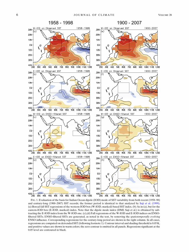
FIG. 1. Evaluation of the basis for Indian Ocean dipole (IOD) mode of SST variability from both recent (1958–98)

and century-long (1900–2007) SST records; the former period is identical to that analyzed by Saji et al. (1999).

(a) Boreal fall SST regressions of the western-IOD box (W-IOD, marked) based SST index. (b) As in (a), but for the

eastern-IOD box (E-IOD, marked) index. Note that the dipole mode index (DMI; Saji et al.) is obtained by sub-

tracting the E-IOD index from theW-IOD one. (c),(d) Fall regressions of theW-IOD and E-IOD indices on ENSO-

filtered SSTs; ENSO-filtered SSTs are generated, as noted in the text, by removing the spatiotemporally evolving

ENSO influence. Corresponding regressions for the century-long period are shown in the right column. In all cases,

regressions are computed on detrended SST (following footnote 1). Contour interval and shading threshold is 0.05K,

and positive values are shown in warm colors; the zero contour is omitted in all panels. Regressions significant at the

0.05 level are contoured in black.

6 JOURNAL OF CL IMATE VOLUME 28

influence, are referred to as filtered SSTs. The analysis of

filtered SSTs in the Saji et al. period (1958–98) shows the

western dipole center to be nonviable: regressions of

the western IOD box have no footprint whatsoever over

the eastern box (Fig. 1c), and likewise for regressions

of the eastern IOD box (Fig. 1d) over the other region.

The eastern box is again found more connected to the

south-central equatorial IO SSTs,3 albeit more weakly

than before. The century-long (1900–2007) analysis of

filtered SSTs (Figs. 1g,h) corroborates the shorter-period

findings, as does an inspection of the related correlation

maps (not shown).

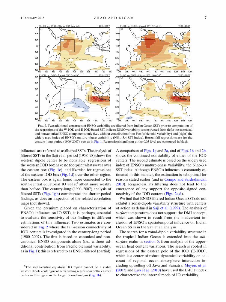
Given the premium placed on characterization of

ENSO’s influence on IO SSTs, it is, perhaps, essential

to evaluate the sensitivity of our findings to different

estimations of this influence. Two estimates are con-

sidered in Fig. 2 where the fall-season connectivity of

IOD centers is investigated in the century-long period

(1900–2007). The first is based on canonical and non-

canonical ENSO components alone (i.e., without ad-

ditional contribution from Pacific biennial variability,

as in Fig. 1); this is referred to as ENSO-filtered (partial).

A comparison of Figs. 1g and 2a, and of Figs. 1h and 2b,

shows the continued nonviability of either of the IOD

centers. The second estimate is based on the widely used

index of ENSO’s mature-phase variability, the Niño-3.4SST index. Although ENSO’s influence is commonly es-

timated in this manner, the estimation is suboptimal for

reasons stated earlier (and in Compo and Sardeshmukh

2010). Regardless, its filtering does not lead to the

emergence of any support for opposite-signed con-

nectivity of the IOD centers (Figs. 2c,d).

We find that ENSO-filtered IndianOcean SSTs do not

exhibit a zonal-dipole variability structure with centers

of action as defined in Saji et al. (1999). The analysis of

surface temperature does not support the DMI concept,

which was shown to result from the inadvertent in-

clusion of ENSO’s spatiotemporal influence on Indian

Ocean SSTs in the Saji et al. analysis.

The search for a zonal-dipole variability structure in

the tropical Indian Ocean is extended into the sub-

surface realm in section 5, from analysis of the upper-

ocean heat content variations. The search is rooted in

regressions of the eastern pole of the IOD (E-IOD),

which is a center of robust dynamical variability on ac-

count of regional ocean–atmosphere interaction in-

cluding upwelling off Java and Sumatra. Meyers et al.

(2007) and Luo et al. (2010) have used the E-IOD index

to characterize the internal mode of IO variability.

FIG. 2. Two additional constructs of ENSO variability are filtered from Indian Ocean SSTs prior to computation of

the regressions of theW-IOD and E-IODbased SST indices: ENSO variability is constructed from (left) the canonical

and noncanonical ENSO components only (i.e., without contribution from Pacific biennial variability) and (right) the

widely used index of ENSO’s mature-phase variability (Niño-3.4 SST index). Boreal fall regressions are for thecentury-long period (1900–2007); rest as in Fig. 1. Regressions significant at the 0.05 level are contoured in black.

3 The south-central equatorial IO region cannot be a viable

western dipole center given the vanishing regressions of the eastern

center in this region in the longer period analysis (Fig. 1h).

1 JANUARY 2015 ZHAO AND N IGAM 7

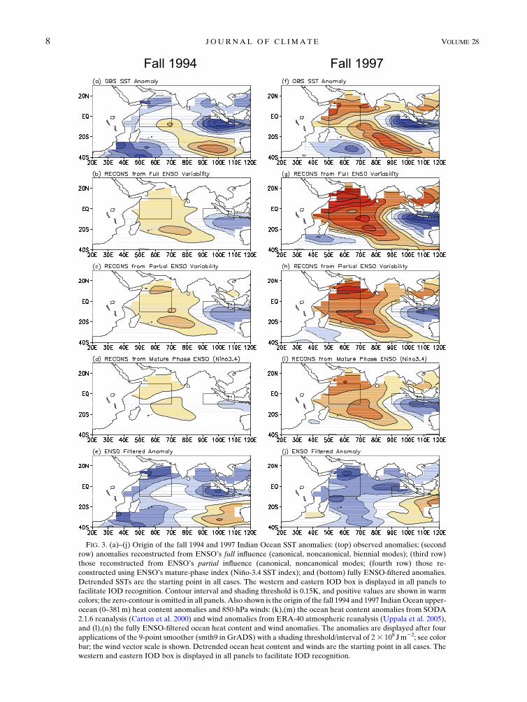
FIG. 3. (a)–(j) Origin of the fall 1994 and 1997 Indian Ocean SST anomalies: (top) observed anomalies; (second

row) anomalies reconstructed from ENSO’s full influence (canonical, noncanonical, biennial modes); (third row)

those reconstructed from ENSO’s partial influence (canonical, noncanonical modes; (fourth row) those re-

constructed using ENSO’s mature-phase index (Niño-3.4 SST index); and (bottom) fully ENSO-filtered anomalies.Detrended SSTs are the starting point in all cases. The western and eastern IOD box is displayed in all panels tofacilitate IOD recognition. Contour interval and shading threshold is 0.15K, and positive values are shown in warmcolors; the zero-contour is omitted in all panels. Also shown is the origin of the fall 1994 and 1997 IndianOcean upper-ocean (0–381m) heat content anomalies and 850-hPa winds: (k),(m) the ocean heat content anomalies from SODA

2.1.6 reanalysis (Carton et al. 2000) and wind anomalies from ERA-40 atmospheric reanalysis (Uppala et al. 2005),

and (l),(n) the fully ENSO-filtered ocean heat content and wind anomalies. The anomalies are displayed after four

applications of the 9-point smoother (smth9 in GrADS) with a shading threshold/interval of 23 108 Jm22; see color

bar; the wind vector scale is shown. Detrended ocean heat content and winds are the starting point in all cases. The

western and eastern IOD box is displayed in all panels to facilitate IOD recognition.

8 JOURNAL OF CL IMATE VOLUME 28

4. The 1994 and 1997 fall SST anomalies: IODevents?

The dipole mode index is strongly positive in the fall

of 1994 and 1997 (Saji et al.1999, their Fig. 1); 1994 was

a weak El Niño year but the 1997 winter saw one of thestrongest warm events on record (NOAA Climate Di-agnostic Bulletin). As ENSO’s influence is aliased in the

DMI definition (cf. Figs. 1 and 2 and related discussion),

it is instructive to examine the structure of both raw

and ENSO-filtered Indian Ocean SST and upper-ocean

(0–381m) heat content anomalies in these two years; the

detrended SSTs and ocean heat content anomalies are

the starting point in both cases. SST anomalies are based

on the century-long (1900–2007) seasonal climatology,

and reconstructed from PCs obtained from an extended-

EOF analysis of SSTs in the same period. The ocean

heat content anomalies are, of necessity, based on the

shorter 41-yr period (1958–98)—the SODAdata period,

which is also Saji et al.’s analysis period. The SST ano-

malies are displayed in Figs. 3a–j, while the heat content

ones are shown in Figs. 3k–n.

The fall 1994 SST anomaly (top panel) is strongly

negative off Sumatra (i.e., over the E-IOD box) but

weaker and ofmixed sign over theW-IODbox. TheDMI

is, interestingly, positive [0.605 (20.03)2 (20.63)] with

similar-signed anomalies in the two IOD boxes. The next

three panels display various estimates of ENSO’s con-

tribution to the fall 1994 SST anomaly. The one obtained

from accounting of the spatiotemporal influence of ca-

nonical and noncanonical ENSO variability, and biennial

variability (i.e., the full ENSO influence) on IO SSTs is

shown in Fig. 3b, while the version without the biennial

component is in Fig. 3c. The IO SST anomaly constructed

from regressions of the Niño-3.4 SST index is shown inFig. 3d. All three estimates of ENSO’s influence on IO

SSTs exhibit a zonal-dipole structure, one that would,

undoubtedly, project on the DMI index. The ENSO-

unrelated IO SST anomaly (i.e., observedminus ENSO’s

full influence) is shown in the bottom panel. The SST

anomalies off Sumatra are not as strong as before

(Fig. 3a) while the ones along the Somali coast and

Arabian Sea are stronger (and of the same sign as the

Sumatra ones) in the ENSO-filtered version (Fig. 3e),

yielding a smaller DMI (0.25) than the one calculated

from unfiltered anomalies (Fig. 3a; 0.60).

The fall 1997 SST anomalies are analyzed in the right

column of Fig. 3. All three estimates of the ENSO

contribution to IO SSTs are now stronger; not surpris-

ing, given the unusually strong 1997 El Niño. The large-scale anomaly structure (zonal dipole) is very similar(except for the amplitude) to that seen in the 1994

FIG. 3. (Continued)

1 JANUARY 2015 ZHAO AND N IGAM 9

contributions (Figs. 3b–d), and also among themselves

(Figs. 3g–i). The ENSO-filtered IO SST anomaly in 1997

(Fig. 3j), interestingly, does not exhibit an impressive

zonal-dipole structure in the IO. The DMI index from

the original (Fig. 3f) and ENSO-filtered SST anomalies

(Fig. 3j) is 1.05 and 20.09, respectively.

A full accounting of ENSO’s contribution to the In-

dian Ocean surface (SST) anomalies in fall 1994 and

1997 suggests a weak IOD event in 1994, and none at all

in 1997. The accounting leads to a rather different as-

sessment in 1997, which was marked as a strongly posi-

tive IOD year in previous analyses (e.g., Saji et al. 1999),

based on DMI computation off raw SST anomalies.

An IOD event was also reported in fall 2006 (Horii

et al. 2008), with aDMI index (0.57) similar to that in fall

1994 (both are weak El Niño years). Reconstruction ofthe IO SST anomalies indicates a strong ENSO contri-bution whose filtering leads to a DMI index of 0.14, ora weak IOD event, much as in fall 1994.

Subsurface anomaly structure

In view of the above-noted disagreement in charac-

terization of the nature and structure of the IO SST

anomalies in fall of 1994, and especially 1997, the related

subsurface anomaly structure is examined in Figs. 3k–n

though plots of the upper-ocean heat content; as before,

both observed and ENSO-filtered versions are shown.

Interestingly, the ENSO-filtered anomaly is nearly in-

distinguishable from the original one in 1994, but very

distinct in 1997 (a strong El Niño year). A zonal-dipolestructure is evident in 1994 but with the western polelocated to the right of the W-IOD box, but no dipolestructure is manifest in the filtered 1997 heat-contentanomaly (Fig. 3n). Strong southeasterlies are present onthe west coast of Sumatra in both cases (Figs. 3k,m),

leading to coastal upwelling and colder SSTs. The

ENSO-filtered winds (Figs. 3l,n) remain southeasterly

but the filtered SSTs off Sumatra are cold only in fall

1994, indicating the significance of other influences on

SST in fall 1997. The similarity of the observed and

ENSO-filtered winds attests to the rather modest in-

fluence of ENSO on Indian Ocean winds (;1–2m s21),

consistent with earlier diagnoses of this signal (e.g.,

Nigam and Shen 1993, see their Fig. 2). The fall 2006

anomalies (not shown) are similar to the 1994 ones in

that their ENSO-filtered versions exhibit weak IOD

variability in SST but robust dipole variability in sub-

surface temperatures.

This limited analysis (two cases) suggests that the

tropical IO basin can exhibit internally generated zonal-

dipole structure, but mainly at the subsurface. Externally

driven IO variability (e.g., from ENSO’s influence), on

the other hand, can generate zonal-dipole type structure

both at the surface and subsurface. If this analysis is

corroborated from additional observational and mod-

eling studies, it would caution against identification of

IOD events from surface analysis.

5. Seasonally evolving subsurface variability in theIndian Ocean: ENSO’s influence

The upper-ocean (0–381m) heat content is an inte-

grated measure of ocean temperature, reflecting input

from surface fluxes, advective transports, and upwelling;

it is thus amore steadymeasure of the upper-ocean state

than SST (Merle 1980). Positive/negative ocean heat

content (OHC) anomalies are generally indicative of

positive (negative) subsurface temperature anomalies,

a deepening (shoaling) thermocline, and at times,

anomalously high (low) SSTs.

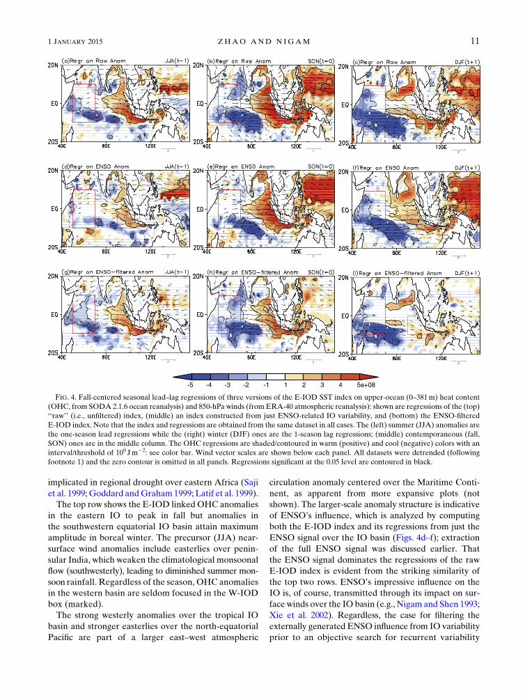
The seasonal evolution of OHC and 850-hPa wind

anomalies associated with fall SST variability at the

E-IOD box—the more viable dipole center—is dis-

played in Fig. 4; the 850-hPa winds, and not surface

winds, are displayed to preclude use of extrapolated

winds over adjoining landmasses. Regressions of three

versions of the E-IOD SST index are shown: lead/lag

regressions of the ‘‘raw’’ (i.e., unfiltered) index are in the

top row, of an index constructed from just ENSO related

IO variability in the middle, and of the ENSO-filtered

E-IOD index are in the bottom row. Seasonal anomalies

are analyzed: The summer [June–August (JJA)] anom-

alies (first column) are the one-season lead regressions

while the winter [December–February (DJF)] ones (last

column) are the one-season lag regressions; contem-

poraneous [fall; i.e., September–November (SON)]

ones are in the middle column.

Regressions of the E-IOD will naturally bring out the

negative phase IOD structure, when temperatures and

OHCoff Sumatra are above normal, and strong westerly

anomalies blow across the western coast of Sumatra

(Fig. 4b); the alongshore winds being from the northwest

lead to coastal downwelling. Equatorial westerlies, on

the other hand, generate downwelling over the open

ocean, leading to thermocline depression over the

eastern equatorial basin. Downwelling equatorial and

coastally trapped Kelvin waves also contribute to the

positive OHC anomalies in this region (Wyrtki 1973;

Clarke and Liu 1993). The southwesterly anomalies

across the southwestern equatorial IO basin generate

upwelling Rossby waves, leading to shallower thermo-

cline and negative OHC anomalies here (Fig. 4b; Meehl

et al. 2003); related regional feedbacks have also been

proposed (e.g., Saji et al. 1999). The off-shore westerly

anomalies (and related moisture transports), evident

especially off Somalia in Fig. 4b, have, of course, been

10 JOURNAL OF CL IMATE VOLUME 28

implicated in regional drought over eastern Africa (Saji

et al. 1999; Goddard andGraham 1999; Latif et al. 1999).

The top row shows the E-IOD linked OHC anomalies

in the eastern IO to peak in fall but anomalies in

the southwestern equatorial IO basin attain maximum

amplitude in boreal winter. The precursor (JJA) near-

surface wind anomalies include easterlies over penin-

sular India, which weaken the climatological monsoonal

flow (southwesterly), leading to diminished summer mon-

soon rainfall. Regardless of the season, OHC anomalies

in the western basin are seldom focused in the W-IOD

box (marked).

The strong westerly anomalies over the tropical IO

basin and stronger easterlies over the north-equatorial

Pacific are part of a larger east–west atmospheric

circulation anomaly centered over the Maritime Conti-

nent, as apparent from more expansive plots (not

shown). The larger-scale anomaly structure is indicative

of ENSO’s influence, which is analyzed by computing

both the E-IOD index and its regressions from just the

ENSO signal over the IO basin (Figs. 4d–f); extraction

of the full ENSO signal was discussed earlier. That

the ENSO signal dominates the regressions of the raw

E-IOD index is evident from the striking similarity of

the top two rows. ENSO’s impressive influence on the

IO is, of course, transmitted through its impact on sur-

face winds over the IO basin (e.g., Nigam and Shen 1993;

Xie et al. 2002). Regardless, the case for filtering the

externally generated ENSO influence from IO variability

prior to an objective search for recurrent variability

FIG. 4. Fall-centered seasonal lead–lag regressions of three versions of the E-IOD SST index on upper-ocean (0–381m) heat content

(OHC, from SODA 2.1.6 ocean reanalysis) and 850-hPa winds (from ERA-40 atmospheric reanalysis): shown are regressions of the (top)

‘‘raw’’ (i.e., unfiltered) index, (middle) an index constructed from just ENSO-related IO variability, and (bottom) the ENSO-filtered

E-IOD index. Note that the index and regressions are obtained from the same dataset in all cases. The (left) summer (JJA) anomalies are

the one-season lead regressions while the (right) winter (DJF) ones are the 1-season lag regressions; (middle) contemporaneous (fall,

SON) ones are in the middle column. The OHC regressions are shaded/contoured in warm (positive) and cool (negative) colors with an

interval/threshold of 108 Jm22: see color bar. Wind vector scales are shown below each panel. All datasets were detrended (following

footnote 1) and the zero contour is omitted in all panels. Regressions significant at the 0.05 level are contoured in black.

1 JANUARY 2015 ZHAO AND N IGAM 11

structures across this basin is reinforced by the above

analysis.

Finally, the structure of internally generated vari-

ability in the IO basin is revealed in Figs. 4g–i (bottom

row) via regressions of the E-IOD index; the index and

regressions are both obtained from ENSO-filtered IO

variability. Not unexpectedly, OHC anomalies are now

present primarily in the IO basin. But, somewhat sur-

prisingly, a coherent dipole structure is manifest, with

the western basin anomalies somewhat better posi-

tioned vis-à-vis the W-IOD box. The analysis supportsthe finding of the previous section, namely that internallygenerated variability in the tropical IO basin can exhibita zonal-dipole structure at the subsurface.

6. Recurrent modes of variability in filtered IndianOcean SSTs

An objective search for the recurrent modes of vari-

ability of Indian Ocean SSTs is undertaken, in contrast to

the analysis of variability patterns in the preceding sec-

tions. The distinction between mode and pattern is im-

portant as the former refers to a unique spatiotemporal

variability structure while the latter to just a spatial pat-

tern of variability that is linked, potentially, with more

than one time scale. Another difference is that previous

analyses factored for just ENSO’s influence on the IO

basin, while the present one will also factor for the in-

fluence of Pacific decadal SST variability. Finally, the

previous sectionswere too focused on theE-IODbecause

it was themore viable of the IODpoles, but it is unclear if

the E-IOD region would emerge as a key variability

center in an objective analysis of filtered IO SSTs.

a. SST filtering

Recurrent spatiotemporal structure of SST variability

in the Indian Ocean is analyzed after filtering the in-

fluence of both interannual and decadal Pacific SST

variability. The influence of ENSO variability was esti-

mated in section 3; the impact of decadal variability is,

likewise, estimated from regressions of the pan-Pacific

and North Pacific PCs (GN2008). The first mode, with

a horseshoe structure in the Pacific, exhibits connections

to the tropical–subtropical Atlantic resembling the

AMO. The second, capturing the 1976/77 climate shift,

is similar to Pacific decadal oscillation (Mantua et al.

1997) in structure but with interesting links to the IO

SSTs (cf. Fig. 12 in GN2008). The SST record was al-

ready detrended earlier using regressions of the non-

stationary SST secular trend (cf. footnote 1); this mode

captures the widespread but nonuniform warming of all

basins along with a sliver of cooling in the central

equatorial Pacific.4

b. Analysis technique

The filtered, seasonal SST anomalies during 1902–

2007 were analyzed in the Indian Ocean basin (408S–308N, 208–1208E) using the extended-EOF technique

(Weare and Nasstrom 1982); seven-season-long anom-

aly sequences were targeted in the primary analysis (T0)

where two leading loading vectors are rotated. Robust-

ness of the variability modes was ascertained by per-

turbing the primary analysis: no rotation of loading

vectors (T1), rotation of three loading vectors (T2),

shorter (five season long) sampling window (T3), Indian

Ocean SSTs additionally filtered for Atlantic’s influence

(T4), and Indian Ocean SSTs are only detrended but not

filtered for any external influences (T5); all are listed in

Table 1.

Table 2 describes the sensitivity analysis results, in-

cluding temporal correlation of the PCs of the primary

and perturbed analyses. An observational realization of

the mode is the ultimate proof of its physicality. But it is

seldom that observed anomalies are composed of just

one mode of variability (i.e., with all other modes sup-

pressed at that time); of course, should this happen, an

observational ‘‘analog’’ of that mode is encountered.

The number of observational analogs of an extracted set

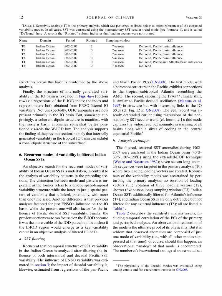
TABLE 1. Sensitivity analysis: T0 is the primary analysis, which was perturbed as listed below to assess robustness of the extracted

variability modes. In all cases, SST was detrended using the nonstationary SST secular trend mode (see footnote 1), and is called

‘‘DeTrend’’ here. A zero in the ‘‘Rotated’’ column indicates that loading vectors were not rotated.

Name Domain Period Rotated Sampling window SST

T0 Indian Ocean 1902–2007 2 7-season DeTrend, Pacific basin influence

T1 Indian Ocean 1902–2007 0 7-season DeTrend, Pacific basin influence

T2 Indian Ocean 1902–2007 3 7-season DeTrend, Pacific basin influence

T3 Indian Ocean 1902–2007 0 5-season DeTrend, Pacific basin influence

T4 Indian Ocean 1902–2007 0 7-season DeTrend, Pacific and Atlantic basin influences

T5 Indian Ocean 1902–2007 0 7-season DeTrend

4 The physicality of the decadal modes was evaluated using

analog counts and fish recruitment records in GN2008.

12 JOURNAL OF CL IMATE VOLUME 28

ofmodes in the anomaly record is one objectivemeasure

of the ‘‘physicality’’ of that extraction, and the primary

analysis is chosen in this manner. An observed anomaly

will be deemed a modal analog if any one PC is larger

than all others in that analysis by at least one unit of

magnitude; note that PCs are orthonormal with or

without rotation. The identification is objective and

easily implemented, and Table 3 lists the number of

analogs in the six analyses (T0–T5): Considering just the

first two PCs, 128 seasonal anomalies (out of the 424

analyzed) are found to be analogs of the first or second

mode in the T0 analysis.

c. Analysis results

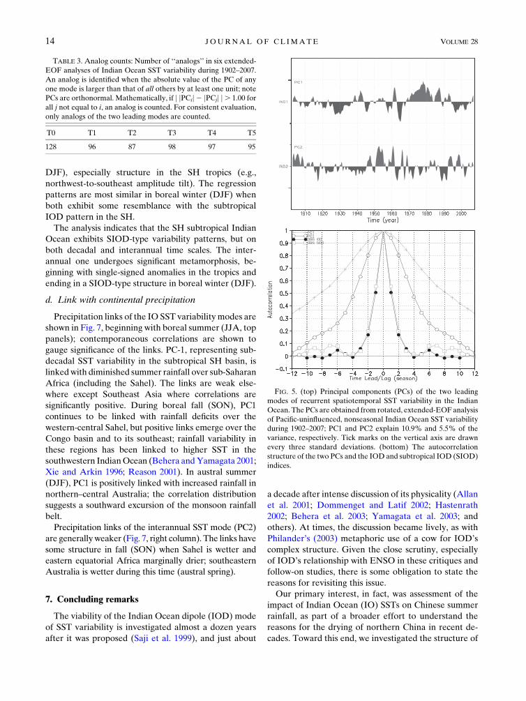
The two leading PCs from the primary analysis (T0)

are shown in Fig. 5a. The leading PC accounts for;11%

of the variance, and represents subdecadal variability

with a notable warm phase in the 1970s–1980s. As seen

later (Fig. 6), the represented SST variability has a me-

ridional dipole structure with a pronounced southern

pole in the subtropical SouthernHemisphere (SH) basin

(focused southward of Mauritius); this region was

anomalously warm during the 1970s to 1980s. The sec-

ond PC (explaining 5%–6% of variance) represents,

principally, interannual variability; the related loading

vector (Fig. 6) is more tropically focused and resembles

the IOD structure in the western-central basin; the

similarity with IOD ends here, however, as shown and

discussed later. Unlike the leading mode, this one ex-

hibits considerable structural evolution, evolving into

a meridional dipole (with a stronger northern pole) in

the SH tropical–subtropical basin before dissipating

(Fig. 6). Potential links with the IOD and the subtropical

IOD (SIOD; Behera and Yamagata 2001) are investi-

gated in Figs. 5b and 6.

The autocorrelation structure of the PCs is examined

in Fig. 5b to estimate the modal time scale; a conserva-

tive estimate follows from the temporal distance of

points where autocorrelation is e21 (’0.37), yielding;6

years for PC1 and 2–3 years for PC2. The autocorrela-

tion structure of the IOD and SIOD indices is also dis-

played in Fig. 5b, for context; both, evidently, represent

much shorter time scale (;1 yr) variability. The corre-

lation of PC1 and the IOD (SIOD) index is 0.14 (0.47),

significant at the 0.001 level. The corresponding PC2

correlations are 20.11 and 0.22, at the 0.05 significance

level. The IOD is thus unrelated to the extracted modes

which exhibit some pattern (but not time scale) simi-

larity to SIOD variability.

Spatiotemporal evolution of the SST variability

modes in the T0 analysis is displayed in the first two

columns of Fig. 6. Seasonal lead–lag regressions of the

fall-season (SON) PCs are shown in order to compare

with the IOD pattern (third column), which is robust in

fall; the fourth column depicts evolution of the sub-

tropical IOD using its winter (DJF)-based index. The

five-season evolution (time running downward) clearly

conveys the variability time scales: significantly longer

than five seasons for PC1, just about this period for PC2,

and shorter than five seasons for both IOD and SIOD,

consistent with the autocorrelation analysis (Fig. 5b).

The evolution of the leading mode is not seasonally

sensitive in view of its;6-yr time scale but others are, as

manifest from the regressions centered on other seasons

(not shown). As noted earlier, the leading mode is fo-

cused in the SH with large amplitudes in the western

subtropics. The second mode, in contrast, has footprints

in the northern basin as well, and shows significant

spatiotemporal development: evolving from a single-

signed anomaly pattern in the tropics in spring–fall into

ameridional dipole in the SH subtropics in boreal winter

(DJF); note the similarity of the winter patterns in the

SH.5 The secondmode dissipates by the following spring

[March–May (MAM)] whereas the first mode shows no

such sign.

A comparison of columns 2 and 3 indicates both

similarities and differences between the second mode of

this analysis and the IOD. Key differences include the

lack of modal amplitude in the western basin (including

Arabian Sea) in fall (SON) and the absence of a zonal-

dipole structure in the tropics (e.g., no modal amplitude

off Sumatra). The similarity accrues from the amplitude

focus in the central basin in boreal fall–winter (SON,

TABLE 2. Sensitivity results: Column 1 shows the leading modes identified in the primary analysis (T0); numbers following the name

indicate the percentage variance explained by the mode and its rank, respectively. Columns 2–6 list attributes of the leading modes in the

five sensitivity tests (T1–T5), with the three-slash numbers indicating correlation between the test case and primary analysis PC, the

percentage variance explained by that mode, and its rank in the test analysis. Asterisks indicate ‘‘no match.’’ All correlation coefficients

are significant at the 0.001 level.

T0 T1 T2 T3 T4 T5

IND1/10.9/1 0.96/11.4/1 0.98/10.3/1 0.94/12.6/1 0.92/10.9/1 0.67/6.7/3

IND2/5.5/2 0.96/5.0/2 0.82/5.1/3 0.88/6.3/2 0.71/5.2/2 *

5An extended-EOF analysis is well positioned to distinguish

variability structures having similar spatial footprint but different

time scales and evolution.

1 JANUARY 2015 ZHAO AND N IGAM 13

DJF), especially structure in the SH tropics (e.g.,

northwest-to-southeast amplitude tilt). The regression

patterns are most similar in boreal winter (DJF) when

both exhibit some resemblance with the subtropical

IOD pattern in the SH.

The analysis indicates that the SH subtropical Indian

Ocean exhibits SIOD-type variability patterns, but on

both decadal and interannual time scales. The inter-

annual one undergoes significant metamorphosis, be-

ginning with single-signed anomalies in the tropics and

ending in a SIOD-type structure in boreal winter (DJF).

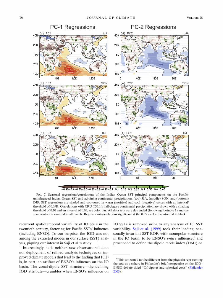
d. Link with continental precipitation

Precipitation links of the IO SST variability modes are

shown in Fig. 7, beginning with boreal summer (JJA, top

panels); contemporaneous correlations are shown to

gauge significance of the links. PC-1, representing sub-

decadal SST variability in the subtropical SH basin, is

linkedwith diminished summer rainfall over sub-Saharan

Africa (including the Sahel). The links are weak else-

where except Southeast Asia where correlations are

significantly positive. During boreal fall (SON), PC1

continues to be linked with rainfall deficits over the

western-central Sahel, but positive links emerge over the

Congo basin and to its southeast; rainfall variability in

these regions has been linked to higher SST in the

southwestern IndianOcean (Behera andYamagata 2001;

Xie and Arkin 1996; Reason 2001). In austral summer

(DJF), PC1 is positively linked with increased rainfall in

northern–central Australia; the correlation distribution

suggests a southward excursion of the monsoon rainfall

belt.

Precipitation links of the interannual SST mode (PC2)

are generallyweaker (Fig. 7, right column). The links have

some structure in fall (SON) when Sahel is wetter and

eastern equatorial Africa marginally drier; southeastern

Australia is wetter during this time (austral spring).

7. Concluding remarks

The viability of the Indian Ocean dipole (IOD) mode

of SST variability is investigated almost a dozen years

after it was proposed (Saji et al. 1999), and just about

a decade after intense discussion of its physicality (Allan

et al. 2001; Dommenget and Latif 2002; Hastenrath

2002; Behera et al. 2003; Yamagata et al. 2003; and

others). At times, the discussion became lively, as with

Philander’s (2003) metaphoric use of a cow for IOD’s

complex structure. Given the close scrutiny, especially

of IOD’s relationship with ENSO in these critiques and

follow-on studies, there is some obligation to state the

reasons for revisiting this issue.

Our primary interest, in fact, was assessment of the

impact of Indian Ocean (IO) SSTs on Chinese summer

rainfall, as part of a broader effort to understand the

reasons for the drying of northern China in recent de-

cades. Toward this end, we investigated the structure of

FIG. 5. (top) Principal components (PCs) of the two leading

modes of recurrent spatiotemporal SST variability in the Indian

Ocean. The PCs are obtained from rotated, extended-EOF analysis

of Pacific-uninfluenced, nonseasonal Indian Ocean SST variability

during 1902–2007; PC1 and PC2 explain 10.9% and 5.5% of the

variance, respectively. Tick marks on the vertical axis are drawn

every three standard deviations. (bottom) The autocorrelation

structure of the two PCs and the IOD and subtropical IOD (SIOD)

indices.

TABLE 3. Analog counts: Number of ‘‘analogs’’ in six extended-

EOF analyses of Indian Ocean SST variability during 1902–2007.

An analog is identified when the absolute value of the PC of any

one mode is larger than that of all others by at least one unit; note

PCs are orthonormal. Mathematically, if j jPCij2 jPCjj j. 1.00 for

all j not equal to i, an analog is counted. For consistent evaluation,

only analogs of the two leading modes are counted.

T0 T1 T2 T3 T4 T5

128 96 87 98 97 95

14 JOURNAL OF CL IMATE VOLUME 28

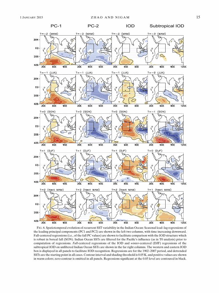
FIG. 6. Spatiotemporal evolution of recurrent SST variability in the IndianOcean: Seasonal lead–lag regressions of

the leading principal components (PC1 and PC2) are shown in the left two columns, with time increasing downward.

Fall-centered regressions (i.e., of the fall PC values) are shown to facilitate comparison with the IOD structure which

is robust in boreal fall (SON). Indian Ocean SSTs are filtered for the Pacific’s influence (as in T0 analysis) prior to

computation of regressions. Fall-centered regressions of the IOD and winter-centered (DJF) regressions of the

subtropical IOD on unfiltered Indian Ocean SSTs are shown in the far right columns. The western and eastern IOD

box is displayed in all panels to facilitate IOD recognition. Regressions are for the 1902–2007 period, and detrended

SSTs are the starting point in all cases. Contour interval and shading threshold is 0.05K, and positive values are shown

in warm colors; zero-contour is omitted in all panels. Regressions significant at the 0.05 level are contoured in black.

1 JANUARY 2015 ZHAO AND N IGAM 15

recurrent spatiotemporal variability of IO SSTs in the

twentieth century, factoring for Pacific SSTs’ influence

(including ENSO). To our surprise, the IOD was not

among the extracted modes in our surface (SST) anal-

ysis, piquing our interest in Saji et al.’s study.

Interestingly, it is neither new observational data

nor deployment of refined analysis techniques or im-

proved climatemodels that lead to the finding that IOD

is, in part, an artifact of ENSO’s influence on the IO

basin. The zonal-dipole SST structure—the defining

IOD attribute—crumbles when ENSO’s influence on

IO SSTs is removed prior to any analysis of IO SST

variability. Saji et al. (1999) took their leading, sea-

sonally invariant SST EOF, with monopolar structure

in the IO basin, to be ENSO’s entire influence,6 and

proceeded to define the dipole mode index (DMI) on

FIG. 7. Seasonal regressions/correlations of the Indian Ocean SST principal components on the Pacific-

uninfluenced Indian Ocean SST and adjoining continental precipitation: (top) JJA, (middle) SON, and (bottom)

DJF. SST regressions are shaded and contoured in warm (positive) and cool (negative) colors with an interval/

threshold of 0.05K. Correlations with CRU TS3.1’s half-degree continental precipitation are shown with a shading

threshold of 0.10 and an interval of 0.05; see color bar. All data sets were detrended (following footnote 1) and the

zero contour is omitted in all panels. Regressions/correlations significant at the 0.05 level are contoured in black.

6 This too would not be different from the physicist representing

the cow as a sphere in Philander’s brief perspective on the IOD–

ENSO debate titled ‘‘Of dipoles and spherical cows’’ (Philander

2003).

16 JOURNAL OF CL IMATE VOLUME 28

the basis of the second EOF’s structure. As the EOFs are

temporally orthogonal, Saji et al. viewed the IOD (based

on DMI) to be ENSO-independent. ENSO’s full in-

fluence on IO SSTs was, of course, not captured by Saji

et al.’s first mode. Although capturing ENSO’s full in-

fluence is nontrivial, as discussed in GN2008 and Compo

and Sardeshmukh (2010), and earlier in section 3 and 6a

of this study, we show that a zonal-dipole variability

structure is untenable even when a rudimentary estimate

of ENSO’s influence on IO SSTs (from Niño-3.4 SSTindex regressions) is filtered in advance of IO SST vari-ability analysis.Not surprisingly, Dommenget (2011) reached a simi-

lar conclusion, namely that variations of the IO zonal

SST gradient (or DMI) are not independent of ENSO,

using the distinct EOF (DEOF) analysis technique

(Dommenget 2007) where a first-order autoregressive

model is used to generate the null hypothesis for the

EOF patterns. This analysis, like ours, revealed no co-

herent connection between the two DMI centers at the

surface. Meyers et al. (2007) also sought to remove the

ENSO signal from the IO SSTs prior to the IO analysis,

using a lagged-EOF technique that seeks to capture

a spatiotemporally evolving signal (e.g., ENSO) as a

single mode. The efficacy of this technique in capturing

ENSO’s complex variability, however, was not assessed

by the authors (e.g., from correlations of the observed

and reconstructed Niño-3.4 SST indices). The methodinvolves restoring phase lags—a daunting task when the

variability mode exhibits multiple time scales, not all of

which are a priori known. Some differences in assess-

ment of the IOD–ENSO relationship among analyses

are thus expected. Note that our extended-EOF analysis

(Weare and Nasstrom 1982) is equivalent to the widely

used multichannel singular spectrum analysis (von

Storch and Zwiers 1999).

Unable to find a zonal-dipole mode of internal vari-

ability at the surface (SST), we extended the search to the

subsurface realm, specifically upper-ocean (0–381m) heat

content (OHC) variations. The search was first conducted

in context of the two recent fall-period IO SST anomalies

(1994 and 1997), both of which are classified as positive

IOD events (e.g., Saji et al. 1999), with a DMI index of

10.60 and 11.05, respectively. Deconstruction of the fall

SST anomalies revealed a DMI index of10.25 and20.09

in the ENSO-filtered SST anomalies (i.e., a weak IOD

event in 1994 and none at all in 1997). Deconstruction of

the OHC anomalies did indicate a zonal-dipole structure

in 1994 but with thewestern pole positioned to the right of

the western IOD box; no dipole was manifest in 1997 in

the ENSO-filtered OHC. This limited analysis suggests

that internally generated variability in the tropical IO

basin can exhibit zonal-dipole structure, but perhaps only

at the subsurface. This finding, based on two cases, was

corroborated from regressions of the E-IOD index (based

on SST anomalies in the eastern IODbox) onOHCover a

40-yr period.

Finally, we report on an objective search for the re-

current modes of variability of IO SSTs from which the

influence of both ENSO and Pacific decadal SST vari-

ability has been removed. The reported search for the

internally generated modes of IO variability is different

from prior analyses that typically focus on recurrent

spatial patterns, in contrast with spatiotemporal patterns

in the present search. Interestingly, none of the ex-

tracted modes was found to exhibit a zonal-dipole

structure in SST. The second leading mode does have

a dipole-like structure but in the meridional direction

and in boreal fall/winter, when it resembles the sub-

tropical IOD (SIOD) pattern. The resemblance, how-

ever, stops there as this mode’s evolution time scale is

considerably longer than the SIOD’s. The seasonally

evolving continental precipitation links of the two SST

variability modes contain interesting features over sub-

Saharan Africa, the Congo basin, and northern-central

Australia.

Our study calls into question the edifice built on the

DMI index, including constructs such as the Equatorial

Indian Ocean Oscillation (EQUINOO)–(IOD-related

zonal surface wind variability at the equator (Gadgil et al.

2004).

Acknowledgments. The authors thank Bin Guan

(NASA/JPL) and Alfredo Ruiz-Barradas (University

of Maryland) for advice and technical help with data

analysis. This work is part of the doctoral dissertation of

the first author.

REFERENCES

Allan, R. J., and Coauthors, 2001: Is there an Indian Ocean dipole

and is it independent of the El Niño–Southern Oscillation?

CLIVAR Exchanges, No. 6, International CLIVAR Project

Office, Southampton, United Kingdom, 18–22.

Ashok, K., Z. Y. Guan, and T. Yamagata, 2003: A look at the re-

lationship between the ENSO and the Indian Ocean dipole.

J. Meteor. Soc. Japan, 81, 41–56, doi:10.2151/jmsj.81.41.

——, S. K. Behera, S. A. Rao, H. Y.Weng, and T. Yamagata, 2007:

El Niño Modoki and its possible teleconnection. J. Geophys.

Res., 112, C11007, doi:10.1029/2006JC003798.

Baquero-Bernal, A., M. Latif, and S. Legutke, 2002: On dipolelike

variability of sea surface temperature in the tropical IndianOcean.

J. Climate, 15, 1358–1368, doi:10.1175/1520-0442(2002)015,1358:

ODVOSS.2.0.CO;2.

Behera, S. K., and T. Yamagata, 2001: Subtropical SST dipole

events in the southern Indian Ocean. Geophys. Res. Lett., 28,327–330, doi:10.1029/2000GL011451.

——, R. Krishnan, and T. Yamagata, 1999: Unusual ocean–

atmosphere conditions in the tropical Indian Ocean during

1 JANUARY 2015 ZHAO AND N IGAM 17

1994. Geophys. Res. Lett., 26, 3001–3004, doi:10.1029/

1999GL010434.

——, S. A. Rao, H. N. Saji, and T. Yamagata, 2003: Comments on

‘‘A cautionary note on the interpretation of EOFs’’. J. Cli-

mate, 16, 1087–1093, doi:10.1175/1520-0442(2003)016,1087:

COACNO.2.0.CO;2.

——, J. J. Luo, S.Masson, S. A. Rao, H. Sakuma, and T. Yamagata,

2006: A CGCM study on the interaction between IOD and

ENSO. J. Climate, 19, 1688–1705, doi:10.1175/JCLI3797.1.

Carton, J. A., and B. S. Giese, 2008: A reanalysis of ocean climate

using Simple Ocean Data Assimilation (SODA). Mon. Wea.

Rev., 136, 2999–3017, doi:10.1175/2007MWR1978.1.

——, G. Chepurin, and X. Cao, 2000: A Simple Ocean Data

Assimilation analysis of the global upper ocean 1950–95.

Part II: Results. J. Phys. Oceanogr., 30, 311–326, doi:10.1175/

1520-0485(2000)030,0311:ASODAA.2.0.CO;2.

Chambers, D., B. Tapley, and R. Stewart, 1999: Anomalous warm-

ing in the Indian Ocean coincident with El Niño. J. Geophys.

Res., 104, 3035–3047, doi:10.1029/1998JC900085.Clarke, A. J., and X. Liu, 1993: Observations and dynamics of

semiannual and annual sea levels near the eastern equatorial

Indian Ocean boundary. J. Phys. Oceanogr., 23, 386–399,

doi:10.1175/1520-0485(1993)023,0386:OADOSA.2.0.CO;2.

Compo, G. P., and P. D. Sardeshmukh, 2010: Removing ENSO-

related variations from the climate record. J. Climate, 23,

1957–1978, doi:10.1175/2009JCLI2735.1.

Dommenget, D., 2007: Evaluating EOF modes against a stochastic

null hypothesis. Climate Dyn., 28, 517–531, doi:10.1007/

s00382-006-0195-8.

——, 2011: An objective analysis of the observed spatial structure

of the tropical Indian Ocean SST variability.Climate Dyn., 36,

2129–2145, doi:10.1007/s00382-010-0787-1.

——,andM.Latif, 2002:Acautionarynoteon the interpretationofEOFs.

J. Climate, 15, 216–225, doi:10.1175/1520-0442(2002)015,0216:

ACNOTI.2.0.CO;2.

——, V. Semenov, and M. Latif, 2006: Impacts of the tropical In-

dian and Atlantic Oceans on ENSO. Geophys. Res. Lett., 33,

L11701, doi:10.1029/2006GL025871.

Frauen, C., and D. Dommenget, 2012: Influences of the tropical

Indian and Atlantic Oceans on the predictability of ENSO.

Geophys. Res. Lett., 39, L02706, doi:10.1029/2011GL050520.

Gadgil, S., P. Vinayachandran, P. Francis, and S. Gadgil, 2004:

Extremes of the Indian summer monsoon rainfall, ENSO and

equatorial Indian Ocean oscillation. Geophys. Res. Lett., 31,

L12213, doi:10.1029/2004GL019733.

Goddard, L., and N. E. Graham, 1999: Importance of the Indian

Ocean for simulating rainfall anomalies over eastern and

southern Africa. J. Geophys. Res., 104, 19 099–19 116,

doi:10.1029/1999JD900326.

Guan, B., and S. Nigam, 2008: Pacific sea surface temperatures in

the twentieth century: An evolution-centric analysis of vari-

ability and trend. J. Climate, 21, 2790–2809, doi:10.1175/

2007JCLI2076.1.

——, and——, 2009: Analysis of Atlantic SST variability factoring

interbasin links and the secular trend: Clarified structure of the

Atlantic multidecadal oscillation. J. Climate, 22, 4228–4240,

doi:10.1175/2009JCLI2921.1.

Hastenrath, S., 2002: Dipoles, temperature gradient, and tropical

climate anomalies. Bull. Amer. Meteor. Soc., 83, 735–738,

doi:10.1175/1520-0477(2002)083,0735:WLACNM.2.3.CO;2.

Horii, T., H. Hase, I. Ueki, and Y. Masumoto, 2008: Oceanic

precondition and evolution of the 2006 Indian Ocean dipole.

Geophys. Res. Lett., 35, L03607, doi:10.1029/2007GL032464.

Huang, B., and J. Shukla, 2007a: Mechanisms for the interannual

variability in the tropical Indian Ocean. Part I: The role of

remote forcing from the tropical Pacific. J. Climate, 20, 2917–

2936, doi:10.1175/JCLI4151.1.

——, and ——, 2007b: Mechanisms for the interannual variability

in the tropical Indian Ocean. Part II: Regional processes.

J. Climate, 20, 2937–2960, doi:10.1175/JCLI4169.1.

Izumo, T., and Coauthors, 2010: Influence of the state of the Indian

Ocean dipole on the following year’s El Niño. Nat. Geosci., 3,

168–172, doi:10.1038/ngeo760.

Jansen, M. F., D. Dommenget, and N. Keenlyside, 2009: Tropical

atmosphere–ocean interactions in a conceptual framework.

J. Climate, 22, 550–567, doi:10.1175/2008JCLI2243.1.

Kug, J.-S., and I.-S. Kang, 2006: Interactive feedback between

ENSO and the Indian Ocean. J. Climate, 19, 1784–1801,

doi:10.1175/JCLI3660.1.

Latif,M., D.Dommenget,M.Dima, andA.Grötzner, 1999: The roleof IndianOcean sea surface temperature in forcingEastAfrican

rainfall anomalies during December–January 1997/98. J. Cli-

mate, 12, 3497–3504, doi:10.1175/1520-0442(1999)012,3497:

TROIOS.2.0.CO;2.

Luo, J. J., S. Behera, Y. Masumoto, H. Sakuma, and T. Yamagata,

2008: Successful prediction of the consecutive IOD in 2006 and

2007. Geophys. Res. Lett., 35, L14S02, doi:10.1029/

2007GL032793.

——, R. Zhang, S. K. Behera, Y. Masumoto, F.-F. Jin, R. Lukas,

and T. Yamagata, 2010: Interaction between El Niño and ex-treme Indian Ocean dipole. J. Climate, 23, 726–742, doi:10.1175/

2009JCLI3104.1.

Mantua, N. J., S. R. Hare, Y. Zhang, J. M. Wallace, and R. C.

Francis, 1997: A Pacific interdecadal climate oscillation

with impacts on salmon production. Bull. Amer. Meteor.

Soc., 78, 1069–1079, doi:10.1175/1520-0477(1997)078,1069:

APICOW.2.0.CO;2.

Meehl, G. A., J. M. Arblaster, and J. Loschnigg, 2003: Coupled

ocean–atmosphere dynamical processes in the tropical Indian

and Pacific Oceans and the TBO. J. Climate, 16, 2138–2158,

doi:10.1175/2767.1.

Merle, J., 1980: Seasonal heat budget in the equatorial

Atlantic Ocean. J. Phys. Oceanogr., 10, 464–469, doi:10.1175/

1520-0485(1980)010,0464:SHBITE.2.0.CO;2.

Meyers, G., P. McIntosh, L. Pigot, and M. Pook, 2007: The years

of El Niño, La Niña, and interactions with the tropicalIndian Ocean. J. Climate, 20, 2872–2880, doi:10.1175/

JCLI4152.1.

Murtugudde, R., J. P. McCreary, and A. J. Busalacchi, 2000:

Oceanic processes associated with anomalous events in the

Indian Ocean with relevance to 1997–1998. J. Geophys. Res.,

105, 3295–3306, doi:10.1029/1999JC900294.

Nicholls, N., and W. Drosdowsky, 2001: Is there an equato-

rial Indian Ocean SST dipole, independent of the El NiñoSouthern Oscillation? Preprints, Conf. on Climate Vari-

ability, the Oceans, and Societal Impacts, Albuquerque,

New Mexico, Amer. Meteor. Soc., 1.9 [Available online

at https://ams.confex.com/ams/annual2001/techprogram/

paper_17337.htm.]

Nigam, S., and H.-S. Shen, 1993: Structure of oceanic and atmo-

spheric low-frequency variability over the tropical Pacific

and Indian Oceans. Part I: COADS observations. J. Cli-

mate, 6, 657–676, doi:10.1175/1520-0442(1993)006,0657:

SOOAAL.2.0.CO;2.

Philander, S. G., 2003: Of dipoles and spherical cows. Bull. Amer.

Meteor. Soc., 84, 1424, doi:10.1175/BAMS-84-10-1424Philander.

18 JOURNAL OF CL IMATE VOLUME 28

Rasmusson, E. M., X. Wang, and C. F. Ropelewski, 1990: The bi-

ennial component of ENSO variability. J. Mar. Syst., 1, 71–96,

doi:10.1016/0924-7963(90)90153-2.

Rayner, N. A., D. E. Parker, E. B. Horton, C. K. Folland, L. V.

Alexander, D. P. Rowell, E. C. Kent, and A. Kaplan, 2003:

Global analyses of sea surface temperature, sea ice, and night

marine air temperature since the late nineteenth century.

J. Geophys. Res., 108, 4407, doi:10.1029/2002JD002670.

Reason, C., 2001: Subtropical Indian Ocean SST dipole events and

southern African rainfall. Geophys. Res. Lett., 28, 2225–2227,

doi:10.1029/2000GL012735.

——, R. Allan, J. Lindesay, and T. Ansell, 2000: ENSO and cli-

matic signals across the Indian Ocean basin in the global

context. Part I: Interannual composite patterns. Int. J. Climatol.,

20, 1285–1327, doi:10.1002/1097-0088(200009)20:11,1285::

AID-JOC536.3.0.CO;2-R.

Saji, N.H., B. N.Goswami, P.N.Vinayachandran, andT.Yamagata,

1999: A dipole mode in the tropical Indian Ocean.Nature, 401,

360–363.

Shinoda, T., H. H. Hendon, and M. A. Alexander, 2004: Surface

and subsurface dipole variability in the Indian Ocean and its

relation with ENSO. Deep Sea Res., 51, 619–635, doi:10.1016/

j.dsr.2004.01.005.

Uppala, S.M., andCoauthors, 2005: TheERA-40Re-Analysis.Quart.

J. Roy. Meteor. Soc., 131, 2961–3012, doi:10.1256/qj.04.176.

von Storch, H., and F. W. Zwiers, 1999: Statistical Analysis in Cli-

mate Research. Cambridge University Press, 484 pp.

Weare,B.C., and J. S.Nasstrom, 1982:Examples of extended empirical

orthogonal function analyses. Mon. Wea. Rev., 110, 481–485,

doi:10.1175/1520-0493(1982)110,0481:EOEEOF.2.0.CO;2.

Webster, P. J., A.M.Moore, J. P. Loschnigg, andR.R. Leben, 1999:

Coupled ocean–atmosphere dynamics in the Indian Ocean

during 1997–98. Nature, 401, 356–360, doi:10.1038/43848.

Wu, R., and B. P. Kirtman, 2004: Understanding the impacts of

the Indian Ocean on ENSO variability in a coupled GCM.

J. Climate, 17, 4019–4031, doi:10.1175/1520-0442(2004)017,4019:

UTIOTI.2.0.CO;2.

Wyrtki, K., 1973: Physical oceanography of the Indian Ocean. The

Biology of the Indian Ocean, Springer, 18–36.

Xie, P., and P. A. Arkin, 1996: Analyses of global monthly precip-

itation using gauge observations, satellite estimates, and nu-

merical model predictions. J. Climate, 9, 840–858, doi:10.1175/1520-0442(1996)009,0840:AOGMPU.2.0.CO;2.

Xie, S.-P., H. Annamalai, F. A. Schott, and J. P. McCreary,

2002: Structure and mechanisms of south Indian Ocean

climate variability. J. Climate, 15, 864–878, doi:10.1175/

1520-0442(2002)015,0864:SAMOSI.2.0.CO;2.

Yamagata, T., S. K. Behera, S. A. Rao, Z. Guan, K. Ashok, and

H. N. Saji, 2003: Comments on ‘‘Dipoles, temperature gradi-

ents, and tropical climate anomalies.’’ Bull. Amer. Meteor.

Soc., 84, 1418–1422, doi:10.1175/BAMS-84-10-1418.

——, ——, J. J. Luo, S. Masson, M. R. Jury, and S. A. Rao, 2004:

Coupled ocean–atmosphere variability in the tropical Indian

Ocean. Ocean–Atmosphere Interaction and Climate Vari-

ability, Geophys. Monogr.,Vol. 147, Amer. Geophys. Union,

189–212.

Yu, J.-Y., and K. M. Lau, 2005: Contrasting Indian Ocean SST

variability with and without ENSO influence: A coupled

atmosphere–ocean GCM study. Meteor. Atmos. Phys., 90,

179–191, doi:10.1007/s00703-004-0094-7.

1 JANUARY 2015 ZHAO AND N IGAM 19