Embed Size (px)
Citation preview
Ž .Journal of Empirical Finance 8 2001 537–572www.elsevier.comrlocatereconbase
The independence axiom and asset returns
Larry G. Epstein), Stanley E. Zin 1
Abstract
This paper integrates models of atemporal risk preference that relax the independenceaxiom into a recursive intertemporal asset-pricing framework. The resulting models areamenable to empirical analysis using market data and standard Euler equation methods. Weare thereby able to provide the first nonlaboratory-based evidence regarding the usefulnessof several new theories of risk preference for addressing standard problems in dynamiceconomics. Using both stock and bond returns data, we find that a model incorporating riskpreferences that exhibit first-order risk aÕersion accounts for significantly more of themean and autocorrelation properties of the data than models that exhibit only second-orderrisk aÕersion. Unlike the latter class of models which require parameter estimates that areoutside of the admissible parameter space, e.g., negative rates of time preference, the modelwith first-order risk aversion generates point estimates that are economically meaningful.We also examine the relationship between first-order risk aversion and models that employexogenous stochastic switching processes for consumption growth. q 2001 Published byElsevier Science B.V.
Keywords: Independence axiom; Asset returns; Risk preference
1. Introduction
The expected utility model of decision making under risk and, particularly, itscornerstone, the independence axiom, have come under attack recently. The
) Corresponding author. Department of Economics, University of Rochester, Rochester, NY 14627,USA.
1 Graduate School of Industrial Administration, Carnegie Mellon University, Pittsburgh, PA 15213and NBER.
0927-5398r01r$ - see front matter q2001 Published by Elsevier Science B.V.Ž .PII: S0927-5398 01 00039-1
( )L.G. Epstein, S.E. ZinrJournal of Empirical Finance 8 2001 537–572538
empirical evidence upon which this criticism is based consists mostly of behav-ioralrexperimental studies where subjects’ choices among hypothetical andror
Žsmall scale gambles are observed e.g., Kahneman and Tversky, 1979; Chew and. Ž .Waller, 1986; Camerer, 1989a,b; Conlisk, 1989 . Machina 1982 surveys much of
the evidence and argues that violations of the independence axiom are bothsystematic and widespread. A number of new theories of choice under uncertaintyhave been developed in an attempt to explain the evidence which contradicts
Žexpected utility theory. Those upon which we focus here are due to Chew 1983,. Ž .1989 and Gul 1991 .
In this paper, we use the general intertemporal asset-pricing model developed inŽ .Epstein and Zin 1989 and aggregate monthly U.S. time-series data for consump-
tion and asset returns as the basis for an empirical examination of the generalizedtheories of Chew and Gul. In common with much of the empirical literature onaggregate consumption and asset returns, we assume the existence of a representa-tive agent, the homotheticity of preferences and the rationality of expectations. Weinquire whether, given these assumptions, relaxing the independence axiom in thedirections defined by Chew and Gul can help account for the time-series data. Toour knowledge, this is the first evidence available regarding the usefulness of thesenewly developed theories of choice for explaining market data. Of course, tests of
Ž .a theory based on behavior in the field as opposed to the laboratory are prone topotentially serious problems such as errors in data measurement and unavoidablejoint hypotheses. Laboratory-based methods, however, also have well-knowndrawbacks and the behavioral evidence is inconclusive. Some recent behavioral
Ž .studies e.g., Camerer, 1989b; Conlisk, 1989; Harrison, 1990 have cast doubtupon the extent and systematic nature of violations of expected utility theory.Thus, we feel that an analysis based upon market data would provide an importantcomplementary piece of evidence regarding the usefulness of the generalizedtheories of choice. Moreover, we suspect that many economists would attach
Ž .greater importance to the question of whether these new theories do or do nothelp to resolve some of the standard problems in economics, than to theirconsistency with laboratory behavior. The explanation of asset returns clearlyqualifies as such a standard problem.
Representative agent models, with preferences represented by the expectedvalue of the discounted sum of within-period utilities, have not performed well in
Žexplaining the behavior of consumption and asset returns over time e.g., Hansen.and Singleton, 1982, 1983; Mehra and Prescott, 1985 . This, in part, motivates the
Ž .work in Epstein and Zin 1989 , which formulates a class of intertemporal utilityfunctions which are recursive, but not necessarily additive or consistent withexpected utility theory. Recursive utility permits some degree of separation in themodeling of risk aversion and intertemporal substitution. In Epstein and ZinŽ .1991 , generalized method of moments estimation procedures are applied to theEuler equations implied by a particular parametric member of this class of utilityfunctions. The results are mixed though some support is provided for the general-
( )L.G. Epstein, S.E. ZinrJournal of Empirical Finance 8 2001 537–572 539
ized specification. The functional form used in that study does not conform withintertemporal expected utility. However, it satisfies the independence axiom forthe set of so-called timeless wealth gambles—those for which all uncertainty isresolved before further consumptionrsavings decisions are made. Since these areprecisely the sort of gambles that are considered in the experimental literature, the
Ž .specification of intertemporal utility that is estimated in Epstein and Zin 1991 isinconsistent with the cited evidence against the independence axiom. This paperfocuses on the empirical gains from further generalizations of intertemporal utilityto specifications in which orderings of timeless wealth gambles conform with thetheories of Chew and Gul and not necessarily with the independence axiom.
The Euler equations implied by a representative agent’s consumptionrportfolioselection problem form the basis for the empirical analysis. We first makegraphical comparisons of the meanrvariance properties of the stochastic discountrates, i.e., the marginal rates of intertemporal substitution, that are implied by theEuler equations for each model. In addition, these meanrvariance properties can
Ž .be used as in Hansen and Jagannathan 1991 to form an informal test of theseasset-pricing models. Second, we provide a more formal statistical analysis basedon the generalized method of moments. Finally, we explore the relationshipbetween the general preference-based models and standard expected utility modelsin which consumption growth rates are subject to exogenous stochastic processswitching.
The paper proceeds as follows. The next two sections lay the groundwork forthe empirical analysis by summarizing and applying the most relevant materialfrom the two literatures on decision theory and intertemporal asset pricing. In
Ž . Ž .Section 2, the Chew 1983, 1989 and Gul 1991 utility functions are described.Section 3 outlines their integration into a recursive model of intertemporal utility
Ž .based on Epstein and Zin 1989 and presents the implied model of asset returns.Section 4 contains the empirical analysis. Section 5 concludes and summarizes thepaper.
2. Certainty equivalents for timeless wealth gambles
In this section, we summarize the relevant aspects of the utility functionsŽ . Ž .proposed by Chew 1983, 1989 and Gul 1991 . These functions represent
preferences over atemporal or one-shot gambles. Integration into a multiperiodsetting is described in the next section.
Ž 1 .Consider a utility function, m, defined on a subset of D R , the set ofqqŽ .cumulative distribution functions cdf’s F, on the positive real line. If x)0, then
Ž .d represents the gamble in which the outcome, x, is certain; d y s0 if y-xx xŽ . nand d y s1 if yGx. Similarly, FsÝ P d represents the gamble in whichx is1 i x i
the outcome, x , is realized with probability, p , is1, 2, . . . , n.i i
( )L.G. Epstein, S.E. ZinrJournal of Empirical Finance 8 2001 537–572540
Only the ordinal properties of m are relevant. Without essential loss ofgenerality, therefore, we can assume that:
m d sx for all x)0. 2.1Ž . Ž .x
As a result, m assigns to any cdf F its certainty equivalent, i.e., that wealth level,x, such that receiving x with certainty is indifferent to the gamble represented byF. Thus, we refer to m as a certainty equivalent function.
Consistent with the relevant empirical literature on intertemporal asset pricingand consumption, we assume that m exhibits constant relative risk aversion. Thatis, for any random variable, x, with cdf Fx:˜ ˜
m F slm F for all l)0. 2.2Ž .Ž . Ž .l x x˜ ˜
The functional forms for m considered in this paper are all special cases of thefollowing, which represents the constant-relative-risk-averse members of the fam-
Ž .ily of semiweighted utility functions studied by Chew 1989 :
f xrm F d F x s0. 2.3Ž . Ž . Ž .Ž .H SW
where f has the form:
wU x Õ x yÕ 1 , xG1Ž . Ž . Ž .Ž .f x s 2.4Ž . Ž .
L½w x Õ x yÕ 1 , xF1.Ž . Ž . Ž .Ž .Under suitable assumptions for the valuation function, Õ, and for the lower and
L U Ž . Ž .upper weight functions, w and w , Eq. 2.3 defines m F implicitly for each cdfŽ .F. Note that m defined in this way satisfies the certainty equivalent condition 2.1
Ž .if f 1 s0.Ž . Ž .Though the general form of Eq. 2.2 has an intuitive interpretation see below ,
we find it instructive to restrict our attention initially to the parametric specializa-tions we will use in our empirical investigation. Accordingly, restrict the valuationand weight functions to have the forms:
x ay1 ra , a/0.Ž .Õ x sŽ . ½ log x , as0,Ž .
wL x sx d and wU x sAx d . 2.5Ž . Ž . Ž .Consider the further parametric restrictions:
0-AF1 and aq2d-1. 2.6Ž .Ž . Ž .In Appendix A, it is shown that the given Eqs. 2.4 – 2.6 , we can find an interval
w x Ž . Ž .a, b , depending on a and d , 0-a-1-b, such that Eq. 2.3 defines m Fw ximplicitly for all cdf’s on the positive real line which have support in a, b .
Furthermore, on this domain, m is strictly monotone in the sense of first-degreestochastic dominance, implies risk aversion in the sense of strict aversion to meanpreserving spreads and exhibits constant relative risk aversion. Finally, under some
( )L.G. Epstein, S.E. ZinrJournal of Empirical Finance 8 2001 537–572 541
auxiliary assumptions, m is well defined and well behaved in the above sense forall cdf’s having finite mean and support in the positive real line. Those assump-tions are:
i ds0 and a-1, orŽ .ii d-0 and 0-aqd-1, orŽ .iii 0-d-1 and aqd-0. 2.7Ž . Ž .
Turn to some special cases. For greater ease of interpretation, we express thefunctional forms for cdf’s having finite support.
( )2.1. Expected utility ds0, As1
With these parameter restrictions, we obtain the linearly homogeneous expectedutility certainty equivalent:
1ra° an p x , a/0,Ž .Ý i i~m p d s 2.8Ž .ÝEU i x iž / ¢exp p log x , as0.Ž .1 Ž .Ý i i
The Arrow-Pratt measure of relative risk aversion equals 1ya .
( )2.2. Weighted utility As1
Ž .The constant relative risk averse from of Chew’s 1983 weighted utility theoryis given by:
1ra° dqap xÝ i i, a/0,
dp xÝ i i~m p d s 2.9Ž .ÝŽ .WU i x i dp x log xŽ .Ý i i iexp , as0.
d¢ p xÝ i i
Ž .Note that m is a single-parameter extension of Eq. 2.8 . The connectionWU
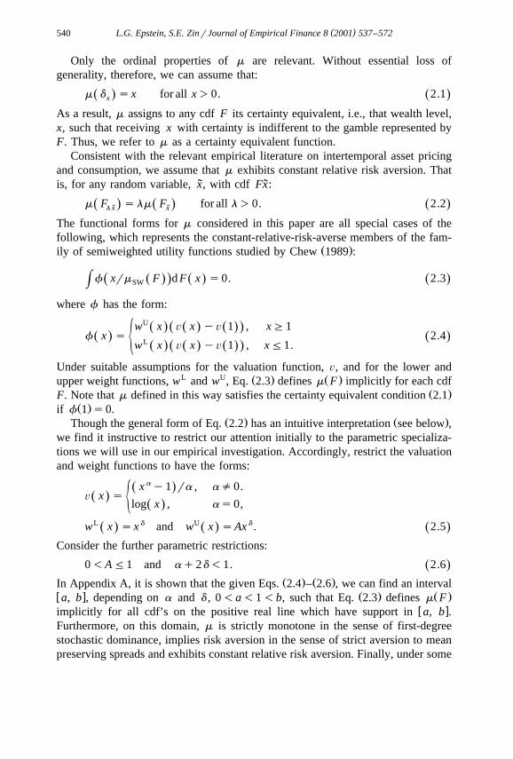
between expected and weighted utility is clarified by the reference to their impliedindifference curves in the probability simplex for the case of three-outcome
Ž .gambles ns3; see Fig. 1 . It is well known that the indifference curves of mEU
are parallel straight lines. For m , indifference curves remain linear; however, ifWU
d/0, they emanate from a finite point, Q, in the plane; Q recedes to infinity asd™0.
In the triangle shown, indifference curves corresponding to higher levels ofŽ .utility are steeper. Such indifference curves are said to fan out. Machina 1982 ,
via his Hypothesis II, points out the close connection between fanning out and theconsistency with Allais-type behavior and the empirical patterns that have come to
( )L.G. Epstein, S.E. ZinrJournal of Empirical Finance 8 2001 537–572542
Fig. 1. Utility function for timeless wealth gambles.
be known as the common consequence effect and the common ratio effect.ŽHowever, recent behavioral evidence regarding fanning out is inconclusive see
.the papers by Camerer and Conlisk . Fortunately, if d)0, weighted utility alsoadmits fanning in, where the point Q lies to the north–east of the triangle and
( )L.G. Epstein, S.E. ZinrJournal of Empirical Finance 8 2001 537–572 543
higher indifference curves are flatter. In Section 4, we are able to exploit theflexibility of weighted utility to investigate whether fanning in or fanning out isindicated by financial market data.
The degree of risk aversion implicit in m is of interest. It follows fromWUŽ .Chew 1983, p. 1083 that the risk premium for a random variable with mean x
2 2 2 Ž . Žand a small variance s x is approximately xs 1yay2d r2. Thus, 1ya
.y2d is a measure of relative risk aversion for small gambles about certainty.Risk aversion increases as a or d falls.
( )2.3. Disappointment aÕersion ds0
Ž . Ž .If we set ds0 in Eq. 2.4 , then Eq. 2.3 implies the following functionalform, which is the contrast-relative-risk-averse specialization of the utility func-
Ž . Ž .tions axiomatized by Gul 1991 : m ÝP d is the unique solution to:DA i x i
ma ras p x araq Ay1 y1 p x ayma ra , a/0,Ž . Ž .Ý ÝDA i i i i DAx -mi DA
log m s p log x q Ay1 y1 p log x y log m , as0.Ž . Ž .Ý ÝDA i i i i DAx -mi DA
2.10Ž .
This functional form provides an alternative single parameter extension ofexpected utility for which As1. The generalization to A-1 admits the follow-ing psychological interpretation. Refer to an outcome x as disappointing if it is1
worse than expected in the sense of being smaller than the certainty equivalent ofŽ .the gamble according to m . In Eq. 2.10 , disappointing outcomes generateDA
negative values for the second summations on the right sides, Ay1 y1)0. Thus,the certainty equivalent is smaller than it would be if As1, reflecting an aversionto disappointment.2
The indifference curves for m in the two-dimensional simplex are shown inDA
Fig. 1. They are linear and emanate from two distinct points Q and QX, both ofwhich recede to infinity as A™1. Thus, indifference curves fan out in the lowerpart of the triangle and otherwise fan in. It is interesting to note in this regard thatthe behavioral evidence supporting fanning out is weaker in the upper triangle than
Ž .in the lower region see Conlisk, for example.
2 There is a similarity in spirit between the structure of m and the hypothesis of Kahneman andDAŽ .Tversky 1979 that individuals evaluate risky prospects in terms of gains and losses relative to a
reference position. Here the reference position is the certainty equivalent of the gamble and the gainsand losses are treated differently in computing the utility of the prospect. Since the reference point isendogenous and depends on the gamble in question, one obtains an ordering based on final wealthpositions. In the cited sources, an exogenously specified reference position is taken to apply to allgambles under consideration and the preference ordering is defined on deviations from that position.
( )L.G. Epstein, S.E. ZinrJournal of Empirical Finance 8 2001 537–572544
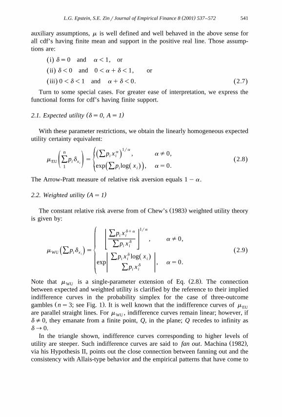
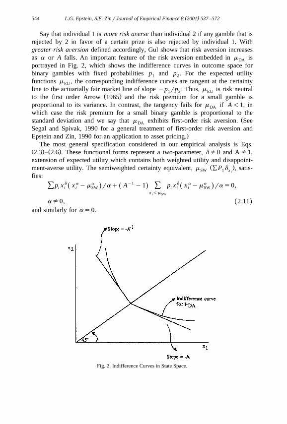
Say that individual 1 is more risk aÕerse than individual 2 if any gamble that isrejected by 2 in favor of a certain prize is also rejected by individual 1. Withgreater risk aÕersion defined accordingly, Gul shows that risk aversion increasesas a or A falls. An important feature of the risk aversion embedded in m isDA
portrayed in Fig. 2, which shows the indifference curves in outcome space forbinary gambles with fixed probabilities p and p . For the expected utility1 2
functions m , the corresponding indifference curves are tangent at the certaintyEU
line to the actuarially fair market line of slope yp rp . Thus, m is risk neutral1 2 EUŽ .to the first order Arrow 1965 and the risk premium for a small gamble is
proportional to its variance. In contrast, the tangency fails for m if A-1, inDA
which case the risk premium for a small binary gamble is proportional to theŽstandard deviation and we say that m exhibits first-order risk aversion. SeeDA
Segal and Spivak, 1990 for a general treatment of first-order risk aversion and.Epstein and Zin, 1990 for an application to asset pricing.
The most general specification considered in our empirical analysis is Eqs.Ž . Ž .2.3 – 2.6 . These functional forms represent a two-parameter, d/0 and A/1,extension of expected utility which contains both weighted utility and disappoint-
Ž .ment-averse utility. The semiweighted certainty equivalent, m ÝP d , satis-SW 1 x1
fies:
p x d x ayma raq Ay1 y1 p x d x ayma ras0,Ž .Ž . Ž .Ý Ýi i i SW i i i SWx -mi SW
a/0, 2.11Ž .and similarly for as0.
Fig. 2. Indifference Curves in State Space.
( )L.G. Epstein, S.E. ZinrJournal of Empirical Finance 8 2001 537–572 545
It is straightforward to provide a disappointment-aversion interpretation forA-1 and also to show that the latter implies first-order risk aversion. Riskaversion increases as a , d or A falls. Finally, a probability simplex indifference
Ž Xmap for m is shown in Fig. 1. Other configurations for Q and Q are possibleSW.though, in all cases, they are collinear with the vertex p s1 . All of the above2
certainty equivalents share the property that indifference curves in the three-out-come probability simplex are straight lines and more generally are hyperplanes inhigher dimensional simplices. Thus, they satisfy the axiom of betweenness, whichis a weakening of the independence axiom proposed and studied by FishburnŽ . Ž . Ž .1983 , Dekel 1986 and Chew 1983, 1989 .
There exist in the literature alternative generalizations of expected utility whichcan explain some of the accumulated behavioral evidence. Two such alternatives
Ž .are prospect theory Kahneman and Tversky, 1979 and rank-dependent or antici-Ž .pated utility theory e.g., Quiggin, 1982; Yaari, 1987; Segal, 1989 . However, in
each case, there are serious difficulties associated with adopting the correspondingfunctional forms in the analysis to follow. For example, prospect theory violatesfirst-degree stochastic dominance unless potential violations are eliminated in apreliminary editing phase; however, a satisfactory specification of the latter is notapparent to us. On the other hand, the central role played by the rank ordering ofoutcomes in the structure of rank-dependent theory makes it computationallyintractable in our multiple asset portfolio choice context. In contrast, there are nosuch difficulties associated with the betweenness-conforming utility functionsadopted here. Whether alternative generalizations of the independence axiom andexpected utility can help to explain the data we study remains a subject for futureresearch.
3. Intertemporal asset pricing with recursive utility
The certainty equivalent functions of the last section are now integrated into aninfinite-horizon, intertemporal setting. Then, we describe the restrictions impliedfor consumption and asset returns by the optimizing behavior of a representative
Ž .agent. The reader is referred to Epstein and Zin 1989 for the details whichsupport the discussion in this section.
There is a single consumption good in each period. In period t, currentconsumption, c , is known with certainty; however, future consumption levels aret
generally uncertain. Thus, intertemporal utility is defined over random consump-tion sequences. It is assumed that the intertemporal utility function is recursive inthe sense that the utility, U , derived from consumption in period t and beyond,t
satisfies the recursive relation:
U sW c , m , tG0, 3.1Ž . Ž .t t t
( )L.G. Epstein, S.E. ZinrJournal of Empirical Finance 8 2001 537–572546
˜ ˜Ž .where m sm U is the certainty equivalent of random future utility, U ,t tq1 tq1
conditional upon period t information.3 The function W is called an aggregatorsince it aggregates current consumption, c , with a certainty-equivalent index oft
the future in order to determine current utility.We restrict W to have the CES form:
1rrr r1yb c qb y , 0/r-1,Ž .W c, y s 3.2Ž . Ž .½exp 1yb log c qb log y , rs0,Ž . Ž . Ž .
where 0-b-1. The utility of deterministic consumption paths is given by theCES intertemporal utility function:
1rp`
t rU s 1yb b c ,Ž . Ý0 tts0
Ž .y1with the elasticity of intertemporal substitution given by ss 1yr and theŽ .constant rate of time preference given by gs 1rb y1. We, therefore, interpret
r as an intertemporal substitution parameter.For the certainty equivalent function, m, we take the semiweighted form m .SW
In our earlier work, we show that m represents the implied preference orderingover timeless wealth gambles, i.e., gambles in which all uncertainty is resolvedbefore further consumption takes place. Moreover, we have already noted that allof the behavioral evidence referred to above regarding individual choice underuncertainty is based on choices among timeless gambles. Thus, the precedingdiscussion of m is pertinent. In particular, risk aversion with respect to timelessSW
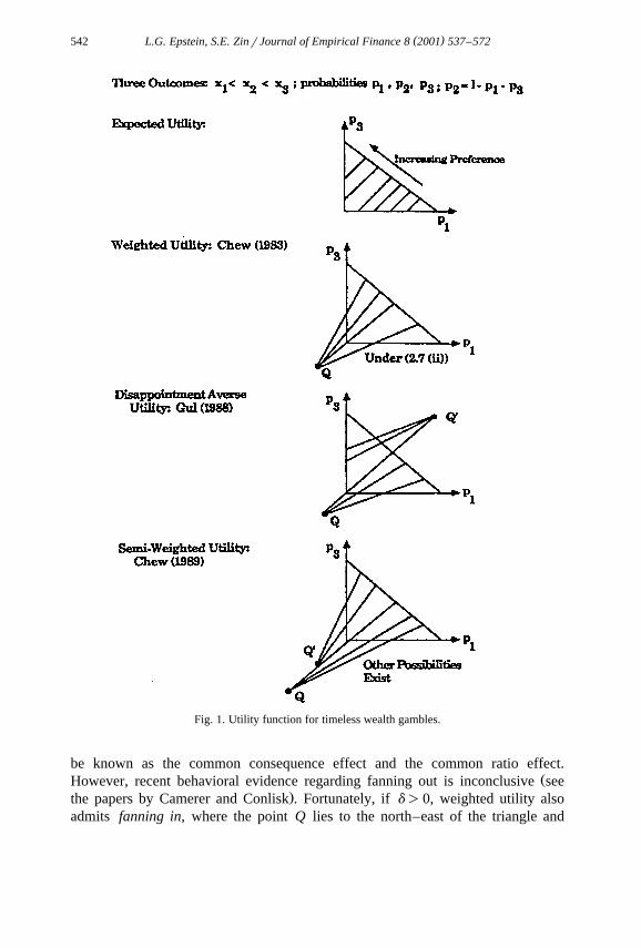
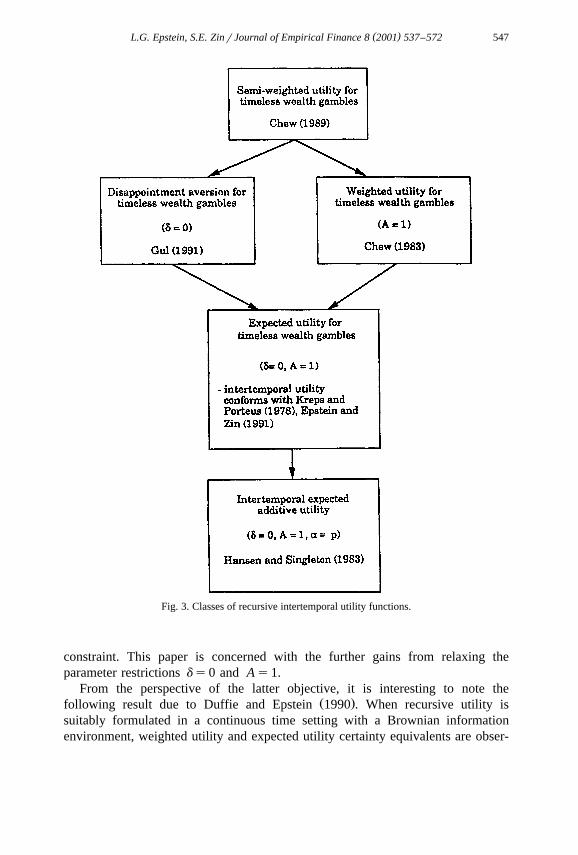
wealth gambles is inversely related to each of the parameters a , A and d .The specializations of m discussed above imply corresponding subclasses ofSW
recursive intertemporal utility functions shown in Fig. 3. Note that the expectedŽ Ž ..utility certainty equivalent specification, m see Eq. 2.8 , does not imply theEU
standard intertemporal utility specification:
1ra`°t a1yb E b c , a/0,Ž . Ý0 t~U s 3.3Ž .ts00
t¢exp 1yb E b log c , as0.Ž . Ž .Ý0 t
Rather, m leads to the infinite-horizon generalization of the intertemporal utilityEUŽ .function of Kreps and Porteus 1978 , explored empirically in Epstein and Zin
Ž . Ž .1991 . The specification Eq. 3.3 corresponds to the added restriction that asr,leaving only a single parameter to model both intertemporal substitution and riskaversion. Our earlier work examined the empirical gains from relaxing this
3 ˜ ˜ ˜ ˜Ž . Ž .Here, we write m U as shorthand for m FU , where FU is the cdf for U conditionaltq1 tq1 tq1 tq1
upon period t information.
( )L.G. Epstein, S.E. ZinrJournal of Empirical Finance 8 2001 537–572 547
Fig. 3. Classes of recursive intertemporal utility functions.
constraint. This paper is concerned with the further gains from relaxing theparameter restrictions ds0 and As1.
From the perspective of the latter objective, it is interesting to note theŽ .following result due to Duffie and Epstein 1990 . When recursive utility is
suitably formulated in a continuous time setting with a Brownian informationenvironment, weighted utility and expected utility certainty equivalents are obser-
( )L.G. Epstein, S.E. ZinrJournal of Empirical Finance 8 2001 537–572548
Žvationally equivalent to one another, whereas and this is strongly suggested,.though not proven by their analysis they are distinguishable from m . Moreover,DA
the essential reason for this difference between m and m seems to be that theDA WU
former alone satisfies first-order risk aversion. Since in the present paper we arenot assuming a Brownian-information, continuous time setting, we cannot rule out
Ž .the potential empirical importance of the generalization from m ds0, As1 ,EUŽ .to m As1 . On the other hand, this result suggests that an empirical analysis,WU
such as ours, should include consideration of certainty equivalents like m thatDA
exhibit first-order risk aversion.We now describe the implications for asset returns and consumption of a
representative agent having recursive intertemporal utility. The agent is assumed tooperate in a standard competitive environment. There are N assets and the ith
� 4asset has positive gross real return, r when held over the interval t, tq1 .˜1, tq1˜Denote by M the return to the market portfolio over the same interval.tq1
In Appendix A, we derive the following Euler equations which representfirst-order conditions for the representative agent’s consumptionrportfolio choiceproblem:
r yr˜ ˜i , tq1 j , tq1E h z I z s0, i/ js1, . . . , N , 3.4Ž .Ž . Ž .˜ ˜t tq1 A tq1 ž /M̃tq1
and
E f z s0, 3.5Ž .Ž .˜t tq1
Ž . Ž .where f is defined by Eqs. 2.4 and 2.5 :Ž . 1r rry1 rM1r r tq1z sb c rc , r/0, 3.6Ž . Ž .tq1 tq1 t
and
x d x a 1qdra ydra , a/0� 4Ž .h x s 3.7Ž . Ž .
d½ x 1qd log x , as0.Ž .Above, E is the expected value operator conditional on period t information andt
I is the indicator function:A
1, x-1,I x sŽ .A ½A , xG1.
For these Euler equations to be valid in the general case where A/1, we mustrestrict the probability distribution of consumption growth and asset returns asdescribed in Appendix A. Sufficient conditions are that for each information set att:
Ž . w xa the conditional distribution of r , . . . , r has compact support in1, tq1 N, tq1
the positive orthant; andŽ . Ž .Ž ry1.rM tq1
1r r
b the conditional distribution of the random variable c rc hastq1 t
a bounded density function.
( )L.G. Epstein, S.E. ZinrJournal of Empirical Finance 8 2001 537–572 549
Ž .According to the model of asset returns represented by Eq. 3.4 , mean excessreturns are determined by covariances of returns with a function of consumptiongrowth and the return to the market. Of course, if As1 and ds0, then one
Ž .obtains the model of asset returns studied in Epstein and Zin 1991 , which has asspecial cases both the static CAPM when as0, and the consumption CAPMwhen asr. These latter restrictions correspond to the standard expected utility
Ž .model studied by Hansen and Singleton 1982, 1983 .To obtain a set of restrictions that apply directly to the levels of individual asset
Ž .returns, multiply Eq. 3.4 by the portfolio weights and sum over all N securitiesto get:
r̃i , tq1E I z h z sE I z h z , is1, . . . , N.Ž . Ž . Ž . Ž .˜ ˜ ˜ ˜t A tq1 tq1 t A tq1 tq1ž /M̃tq1
3.8Ž .Ž . Ž .Now use Eq. 3.5 to rewrite Eq. 3.8 in the form:
r̃i , tq1 dE I z h z sE I z z , 3.9Ž .Ž . Ž . Ž .˜ ˜ ˜ ˜t A tq1 tq1 t A tq1 tq1ž /M̃tq1
which is an equation restricting the level of each return, is1, . . . ; N.
4. Empirical analysis
4.1. The marginal rate of intertemporal substitution
The asset-pricing model derived in the previous sections has the geometricŽ .structure studied by Hansen and Richard 1987 . That is, the model predicts that
equilibrium asset prices are determined by a marginal rate of intertemporalsubstitution, which discounts future asset payoffs before they are averaged acrossstates. For example, we can rewrite our model’s asset-pricing equation for excess
Ž .returns given in Eq. 3.4 as:
E MRS r yr s0, 4.1Ž .˜ ˜Ž .t tq1, t i , tq1 j , tq1
where the marginal rate of intertemporal substitution of c for c is:tq1 t
˜y1MRS sM h z I z , 4.2Ž .Ž . Ž .˜ ˜tq1, t tq1 tq1 A tq1
Ž .for z defined in Eq. 3.6 . The marginal rate of intertemporal substitution for antq1Ž .individual asset return, rather than an excess return, is defined in Eq. 3.9 as:
˜y1h z I z MŽ . Ž .˜ ˜tq1 A tq1 tq1)MRS s .tq1, t dE I z zŽ .˜ ˜t A tq1 tq1
( )L.G. Epstein, S.E. ZinrJournal of Empirical Finance 8 2001 537–572550
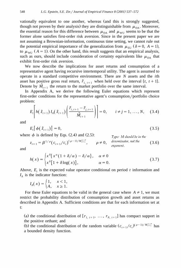
Fig. 4. Hansen-Jagannathan Statistic as RRA varies: s s0.01 and ds0.
We focus on the properties of MRS rather than on MRS) since the latter involvesa conditional expectation which is difficult to compute.4
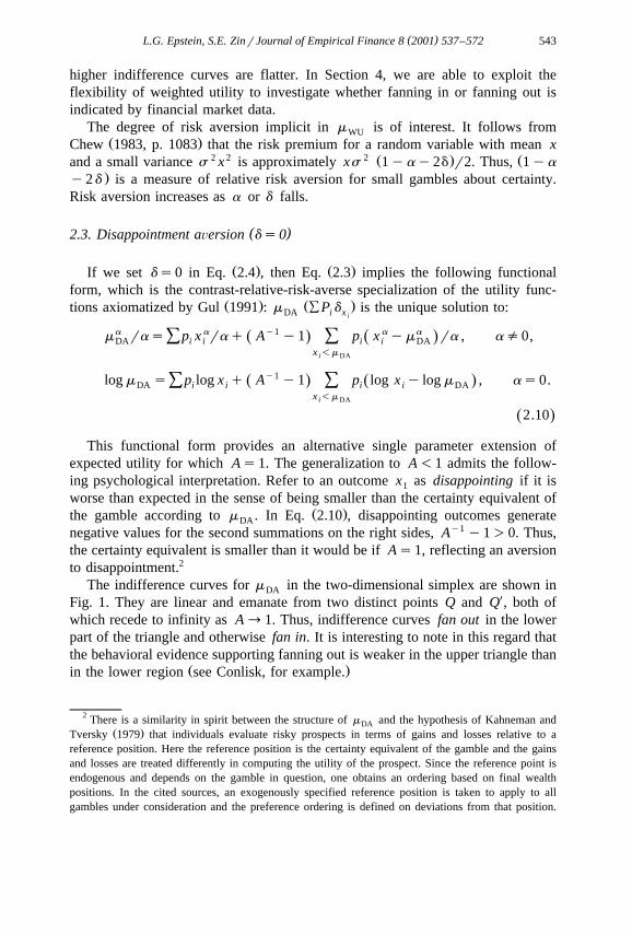
Figs. 4–11 plot the ratio of the estimated standard deviation of MRS to itsmean for various parameter values. Consumption is measured as monthly percapita expenditure in nondurables and services and the monthly NYSE value-weighted return is used to measure the return on the aggregate wealth portfolio5
for the time period 1959:3 to 1986:12. Each figure has five graphs, one for each ofthe five choices for the first-order risk aversion parameter, A. These values rangefrom first-order risk neutrality, As1, to first-order risk aversion corresponding to
Ž .y1As0.3. The elasticity to intertemporal sustitution, ss 1yr , varies across� 4the figures and takes on the values 0.01, 0.1, 0.5, 10 to reflect varying degrees of
substitutability. For Figs. 4–7, the additional risk-aversion parameter for theweighted utility specification, d , is held fixed at zero. Therefore, these figurespertain to the special case of disappointment aversion. The parameter a is varied
Ž .between y29 and 1 so that second-order relative risk aversion varies from 0 to30. In Figs. 8–11, a is fixed at y1 and d is allowed to vary so that the measure
Ž .of local second-order risk aversion, 1yay2d , still varies from 0 to 30. In allof the figures, the discount factor, b , is fixed at 0.9975 corresponding to a 3%annual constant rate of time preference.
4 Ž . )The methods of Gallant et al. 1991 could be used to evaluate MRS by first fitting asemi-nonparametric estimator for the joint distribution of consumption growth and asset returns.
5 Ž .The counsumption data and corresponding implicit price deflator are from Citibase and thevalue-weighted return is from CRSP.
( )L.G. Epstein, S.E. ZinrJournal of Empirical Finance 8 2001 537–572 551
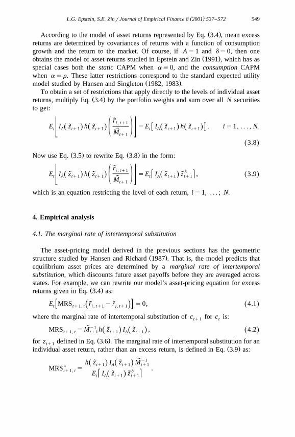
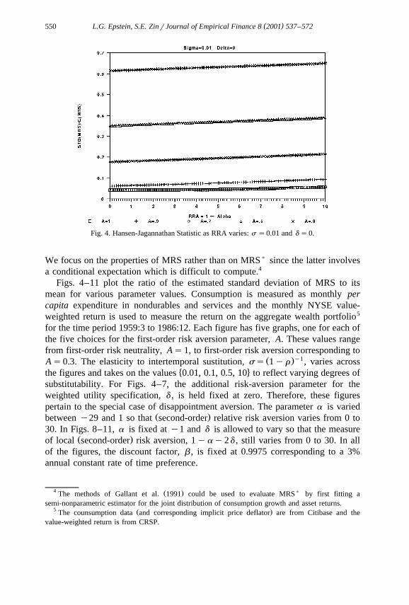
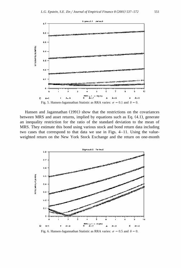
Fig. 5. Hansen-Jagannathan Statistic as RRA varies: s s0.1 and ds0.
Ž .Hansen and Jagannathan 1991 show that the restrictions on the covariancesŽ .between MRS and asset returns, implied by equations such as Eq. 4.1 , generate
an inequality restriction for the ratio of the standard deviation to the mean ofMRS. They estimate this bond using various stock and bond return data includingtwo cases that correspond to that data we use in Figs. 4–11. Using the value-weighted return on the New York Stock Exchange and the return on one-month
Fig. 6. Hansen-Jagannathan Statistic as RRA varies: s s0.5 and ds0.
( )L.G. Epstein, S.E. ZinrJournal of Empirical Finance 8 2001 537–572552
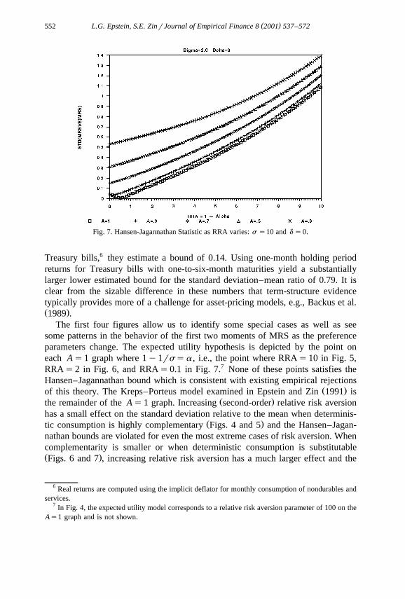
Fig. 7. Hansen-Jagannathan Statistic as RRA varies: s s10 and ds0.
Treasury bills,6 they estimate a bound of 0.14. Using one-month holding periodreturns for Treasury bills with one-to-six-month maturities yield a substantiallylarger lower estimated bound for the standard deviation–mean ratio of 0.79. It isclear from the sizable difference in these numbers that term-structure evidencetypically provides more of a challenge for asset-pricing models, e.g., Backus et al.Ž .1989 .
The first four figures allow us to identify some special cases as well as seesome patterns in the behavior of the first two moments of MRS as the preferenceparameters change. The expected utility hypothesis is depicted by the point oneach As1 graph where 1y1rssa , i.e., the point where RRAs10 in Fig. 5,RRAs2 in Fig. 6, and RRAs0.1 in Fig. 7.7 None of these points satisfies theHansen–Jagannathan bound which is consistent with existing empirical rejections
Ž .of this theory. The Kreps–Porteus model examined in Epstein and Zin 1991 isŽ .the remainder of the As1 graph. Increasing second-order relative risk aversion
has a small effect on the standard deviation relative to the mean when determinis-Ž .tic consumption is highly complementary Figs. 4 and 5 and the Hansen–Jagan-
nathan bounds are violated for even the most extreme cases of risk aversion. Whencomplementarity is smaller or when deterministic consumption is substitutableŽ .Figs. 6 and 7 , increasing relative risk aversion has a much larger effect and the
6 Real returns are computed using the implicit deflator for monthly consumption of nondurables andservices.
7 In Fig. 4, the expected utility model corresponds to a relative risk aversion parameter of 100 on theAs1 graph and is not shown.
( )L.G. Epstein, S.E. ZinrJournal of Empirical Finance 8 2001 537–572 553
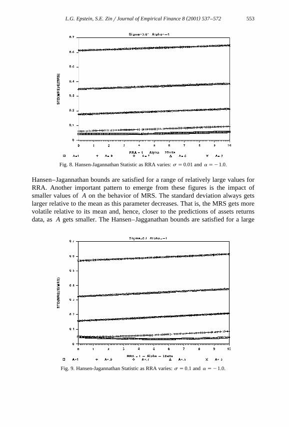
Fig. 8. Hansen-Jagannathan Statistic as RRA varies: s s0.01 and asy1.0.
Hansen–Jagannathan bounds are satisfied for a range of relatively large values forRRA. Another important pattern to emerge from these figures is the impact ofsmaller values of A on the behavior of MRS. The standard deviation always getslarger relative to the mean as this parameter decreases. That is, the MRS gets morevolatile relative to its mean and, hence, closer to the predictions of assets returnsdata, as A gets smaller. The Hansen–Jagganathan bounds are satisfied for a large
Fig. 9. Hansen-Jagannathan Statistic as RRA varies: s s0.1 and asy1.0.
( )L.G. Epstein, S.E. ZinrJournal of Empirical Finance 8 2001 537–572554
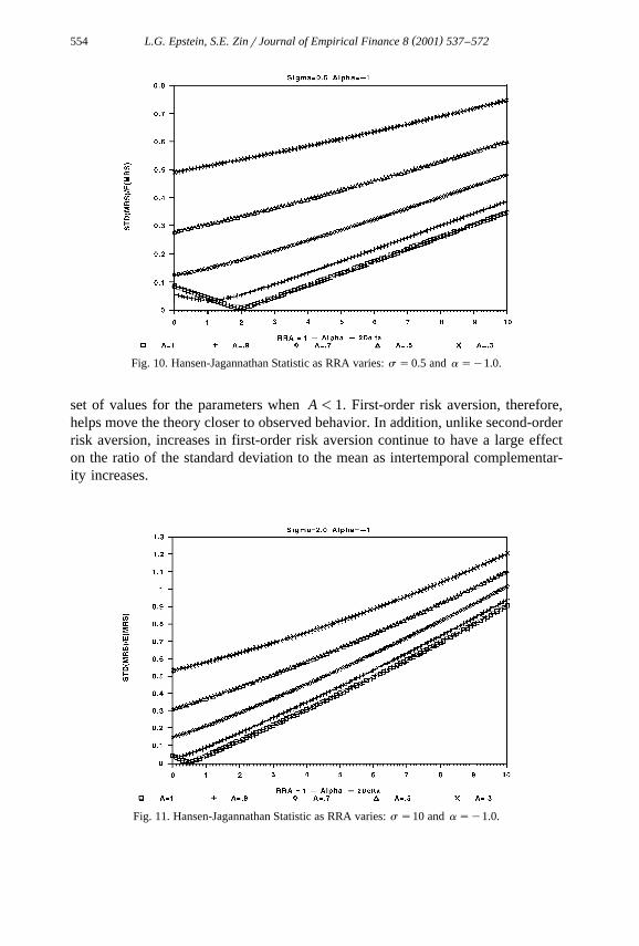
Fig. 10. Hansen-Jagannathan Statistic as RRA varies: s s0.5 and asy1.0.
set of values for the parameters when A-1. First-order risk aversion, therefore,helps move the theory closer to observed behavior. In addition, unlike second-orderrisk aversion, increases in first-order risk aversion continue to have a large effecton the ratio of the standard deviation to the mean as intertemporal complementar-ity increases.
Fig. 11. Hansen-Jagannathan Statistic as RRA varies: s s10 and asy1.0.
( )L.G. Epstein, S.E. ZinrJournal of Empirical Finance 8 2001 537–572 555
The next four figures correspond to weighted and semiweighted utility general-izations in the d dimension. Recall that in these figures, the parameter a is
Žconstrained to equal y1 and the parameter d varies so that 1yay2d the local.measure or second-order relative risk aversion when As1 varies from 0 to 30.
Values along the horizontal axis greater than 2, therefore, imply fanning out, whilevalues less than 2 imply fanning in. The most striking feature of these figures isthe way they closely mimic the previous four figures in which ds0. Thisprovides some confirmation of the theoretical prediction of Duffie and EpsteinŽ .1990 regarding the observational equivalence of weighted utility and Kreps–Porteus utility.
4.2. GMM estimation
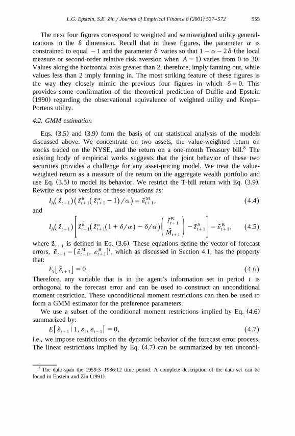
Ž . Ž .Eqs. 3.5 and 3.9 form the basis of our statistical analysis of the modelsdiscussed above. We concentrate on two assets, the value-weighted return onstocks traded on the NYSE, and the return on a one-month Treasury bill.8 Theexisting body of empirical works suggests that the joint behavior of these twosecurities provides a challenge for any asset-pricing model. We treat the value-weighted return as a measure of the return on the aggregate wealth portfolio and
Ž . Ž .use Eq. 3.5 to model its behavior. We restrict the T-bill return with Eq. 3.9 .Rewrite ex post versions of these equations as:
I z z d z a y1 ra s´ M , 4.4Ž .Ž . Ž .˜ ˜ ˜ ˜Ž .A tq1 tq1 tq1 tq1
andBr̃tq1d a d BI z z z 1qdra ydra yz s´ , 4.5Ž . Ž .Ž . Ž .˜ ˜ ˜ ˜ ˜A tq1 tq1 tq1 tq1 tq1ž /M̃tq1
Ž .where z is defined in Eq. 3.6 . These equations define the vector of forecast˜ tq1w M B xTerrors, ´ s ´ , ´ , which as discussed in Section 4.1, has the property˜ ˜tq1 tq1 tq1
that:E ´ s0. 4.6Ž .˜t tq1
Therefore, any variable that is in the agent’s information set in period t isorthogonal to the forecast error and can be used to construct an unconditionalmoment restriction. These unconditional moment restrictions can then be used toform a GMM estimator for the preference parameters.
Ž .We use a subset of the conditional moment restrictions implied by Eq. 4.6summarized by:
E ´ N1, ´ , ´ s0, 4.7Ž .˜tq1 t ty1
i.e., we impose restrictions on the dynamic behavior of the forecast error process.Ž .The linear restrictions implied by Eq. 4.7 can be summarized by ten uncondi-
8 The data span the 1959:3–1986:12 time period. A complete description of the data set can beŽ .found in Epstein and Zin 1991 .
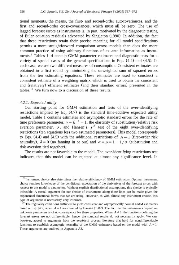
( )L.G. Epstein, S.E. ZinrJournal of Empirical Finance 8 2001 537–572556
tional moments, the means, the first- and second-order autocovariances, and thefirst and second-order cross-covariances, which must all be zero. The use oflagged forecast errors as instruments is, in part, motivated by the diagnostic testing
Ž .of Euler equation residuals advocated by Singleton 1990 . In addition, the factthat these restrictions retain their precise meaning for all model specificationspermits a more straightforward comparison across models than does the morecommon practice of using arbitrary functions of ex ante information as instru-ments.9 Tables 1–4 contain GMM parameter estimates and diagnostic tests for a
Ž . Ž .variety of special cases of the general specifications in Eqs. 4.4 and 4.5 . Ineach case, we use two different measures of consumption. Consistent estimates areobtained in a first round by minimizing the unweighted sum of squared errorsfrom the ten estimating equations. These estimates are used to construct aconsistent estimate of a weighting matrix which is used to obtain the consistent
Ž . Ž .and relatively efficient estimates and their standard errors presented in thetables.10 We turn now to a discussion of these results.
4.2.1. Expected utilityOur starting point for GMM estimation and tests of the over-identifying
Ž .restrictions implied by Eq. 4.7 is the standard time-additive expected utilitymodel. Table 1 contains estimates and asymptotic standard errors for the rate oftime preference parameter, gsby1 y1, the elasticity of substitutionrrelative riskaversion parameter, s , and Hansen’s x 2 test of the eight over-identifying
Ž .restrictions ten equations less two estimated parameters . This model correspondsŽ . Ž . Žto Eqs. 4.4 and 4.5 with the additional restrictions of As1 first-order risk. Ž . Žneutrality , ds0 no fanning in or out and asrs1y1rs substitution and
.risk aversion tied together .The results are not favorable to the model. The over-identifying restrictions test
indicates that this model can be rejected at almost any significance level. In
9 Instrument choice also determines the relative efficiency of GMM estimators. Optimal instrumentchoice requires knowledge of the conditional expectation of the derivatives of the forecast errors withrespect to the model’s parameters. Without explicit distributional assumptions, this choice is typicallyinfeasible. A casual argument for our choice of instruments along these lines can be made given theexponential functional forms that we are using. However, as with almost any instrument choice, thistype of argument is necessarily very informal.
10 The regularity conditions sufficient to yield consistent and asymptotically normal GMM estimatorsŽ . Ž .based on Eq. 4.7 when As1 are covered by Hansen 1982 . The fact that the instruments depend on
unknown parameters is of no consequence for these properties. When A/1, the functions defining theforecast errors are not differentiable; hence, the standard results do not necessarily apply. We can,however, appeal to arguments from the empirical process literature that hold for nondifferentiablefunctions to establish asymptotic normality of the GMM estimators based on the model with A/1.These arguments are outlined in Appendix A3.
( )L.G. Epstein, S.E. ZinrJournal of Empirical Finance 8 2001 537–572 557
Table 1Expected utility
Parameter Nondurables Nondurables and services
Ž . Ž .g y0.0043 0.0022 y0.0132 0.0022Ž . Ž .s 0.2073 0.0094 0.1217 0.0093
� 4 � 4a 1y1rs 1y1rs� 4 � 4d 0 0� 4 � 4A 1 1
2Ž .x 8 35.91 28.08w x w x0.00002 0.0005
Ž 7 . Ž 7 .Moment Fitted value Weight =10 Fitted value Weight =10MŽ . Ž . Ž .E ´ y0.1355 0.0554 0.0012 y0.0697 0.0297 0.0038BŽ . Ž . Ž .E ´ 0.1285 0.0702 0.0001 0.1224 0.0710 0.0001M MŽ . Ž . Ž .E ´ ´ y0.0047 0.0011 12.530 y0.0011 0.0003 125.71y1B BŽ . Ž . Ž .E ´ ´ y0.0483 0.0089 0.1595 y0.0292 0.0062 0.1909y1M BŽ . Ž . Ž .E ´ ´ 0.0180 0.0035 1.4398 0.0077 0.0017 4.8541y1B MŽ . Ž . Ž .E ´ ´ 0.0145 0.0031 1.3587 0.0055 0.0014 5.0839y1M MŽ . Ž . Ž .E ´ ´ y0.0003 0.0010 10.464 y0.0001 0.0003 101.83y2B BŽ . Ž . Ž .E ´ ´ 0.0022 0.0096 0.1413 0.0043 0.0079 0.1501y2M BŽ . Ž . Ž .E ´ ´ y0.0027 0.0029 1.3898 y0.0004 0.0014 4.4613y2B MŽ . Ž . Ž .E ´ ´ 0.0026 0.0030 1.3898 y0.0001 0.0015 4.2351y2
Ž .Asymptotic standard errors, asymptotic p-values, and constrained parameter values are denoted by P ,w x � 4 M BP , and P , respectively. ´ and ´ denote the Euler equation errors for the stock and bond returns.Estimated moments and their standard errors are multiplied by 100. AWeightB is the diagonal elementof the weighting matrix used to compute the estimator.
addition, the estimated rate of time preference is negative and significantly so forone of the consumption measures.
ŽThe lower part of the table contains the estimated moments and their asymp-.totic standard errors and the diagonal elements of the weighting matrix. The
former give us an additional set of tests of the restrictions of the model and thelatter provide some information about how each equation is weighted in thecomputation of the GMM estimator. These help to identify the directions in whichthe model is rejected. The forecast errors exhibit significant first-order autocorrela-tion for both the stock and the bond return equations. Note that the momentsinvolving the bond equation error have a corresponding diagonal element of theweighting matrix that is much smaller than do those for the market equation error.The GMM estimator, therefore, attaches relatively greater weight to the momentsfor the market equation which accounts for the fact that their fitted values aretypically closer to zero than the others.
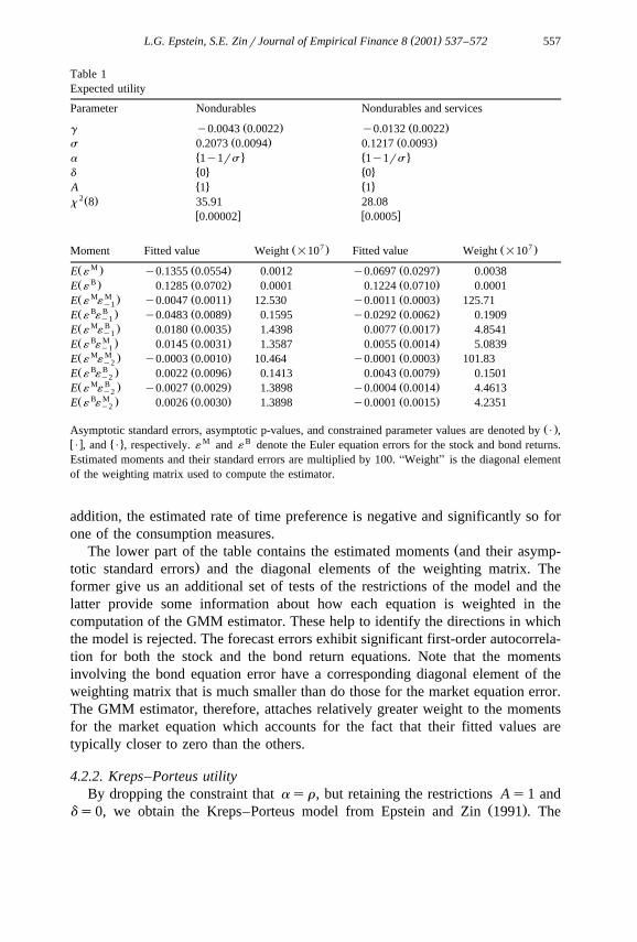
4.2.2. Kreps–Porteus utilityBy dropping the constraint that asr, but retaining the restrictions As1 and
Ž .ds0, we obtain the Kreps–Porteus model from Epstein and Zin 1991 . The
( )L.G. Epstein, S.E. ZinrJournal of Empirical Finance 8 2001 537–572558
results in Table 2 differ numerically from our previous study given the differentmoment restrictions imposed on the estimation problem; however, they exhibit thesame patterns. The substitution elasticity is small as is the coefficient of relativerisk aversion. The rate of time preference is again large and negative. Fornondurable consumption, the x 2 test of the seven over-identifying restrictions hasa p-value of approximately 13%, so it would not be rejected at, say, the 10%level. The nondurables and services measure provides a stronger rejection with ap-value of 1.2%.
The estimated moments for this model have substantially larger standard errorsthan for the expected utility model. As a result, marginal t-tests of the hypothesisthat the moments are individually equal to zero do not reject. The relatively largevalues of the joint test statistic, therefore, come from the correlations across thesemoment equations. Even though these moments are not estimated very precisely,there are a number of changes in the point estimates from those obtained for thepreceding model. The large negative autocorrelation in the bond equation error inthe expected utility model is now a small positive correlation. In fact, almost all ofthe moments involving the bond error have changed sign. The positive averageerror for the bond equation in the expected utility model is now a large negativeaverage error. However, the pattern of attaching relatively more weight to the
Table 2Kreps–porteus utility
Parameter Nondurables Nondurables and services
Ž . Ž .g y0.0077 0.0012 y0.0110 0.0022Ž . Ž .s 0.1550 0.0736 0.1416 0.0632Ž . Ž .a 0.4117 0.2407 1.7113 0.6518
� 4 � 4d 0 0� 4 � 4A 1 1
2Ž . w x w xx 7 11.25 0.128 18.08 0.012
Ž 8. Ž 8.Moment Fitted value Weight =10 Fitted value Weight =10MŽ . Ž . Ž .E ´ y0.0949 0.1643 0.0003 y0.0474 0.0704 0.0013BŽ . Ž . Ž .E ´ y0.2316 0.4584 0.00004 y0.2386 0.4319 0.00004M MŽ . Ž . Ž .E ´ ´ y0.0038 0.0074 5.7739 y0.0012 0.0016 17.674y1B BŽ . Ž . Ž .E ´ ´ 0.0083 0.0544 0.1310 0.0041 0.0538 0.1650y1M BŽ . Ž . Ž .E ´ ´ y0.0018 0.0203 0.8460 y0.0021 0.0094 5.0732y1B MŽ . Ž . Ž .E ´ ´ y0.0049 0.0198 0.9062 y0.0039 0.0090 5.7790y1M MŽ . Ž . Ž .E ´ ´ y0.0002 0.0072 6.7000 y0.0001 0.0014 17.525y2B BŽ . Ž . Ž .E ´ ´ y0.0039 0.0526 0.1334 y0.0063 0.0504 0.1477y2M BŽ . Ž . Ž .E ´ ´ y0.0039 0.0195 0.9603 y0.0014 0.0086 5.2289y2B MŽ . Ž . Ž .E ´ ´ 0.0013 0.0195 0.9324 y0.0010 0.0085 4.9152y2
See Table 1.
( )L.G. Epstein, S.E. ZinrJournal of Empirical Finance 8 2001 537–572 559
moments involving the stock return equation and, hence, providing a better fit forthese moments, is still present.
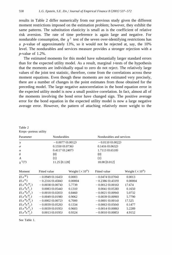
4.2.3. Weighted utilityTable 3 presents results for a model with risk preferences that exhibit first-order
Ž . Ž . Ž .risk neutrality As1 , but are allowed to fan out d-0 or fan in d)0 . Asone might anticipate, given the similarities of the weighted utility model and theKreps–Porteus model found in Section 4.1, the additional parameter introduced bythis specification is not well identified. The value of the objective functiontypically changes very little with substantial changes in the values of a and d .The large standard errors for the estimates of these parameters id further evidenceof this weak identification. The point estimates indicate fanning out for both datasets, however, the large standard errors do not allow fanning in to be rejected.Further, the Kreps–Porteus model cannot be rejected using either a t-test of ds0or a likelihood-ratio-type comparison of x 2 values. The estimate of the rate oftime preference is positive; however, the estimate of the elasticity of substitution issignificantly negative indicating convex utility of deterministic paths. Given theseresults, it is difficult to consider this parameterization to be much of an improve-
Table 3Weighted utility
Parameter Nondurables Nondurables and services
Ž . Ž .g 0.0072 0.0055 0.0067 0.0038Ž . Ž .s y0.3169 0.0450 y0.3656 0.0680
Ž . Ž .a 2.4105 9.7503 8.1409 8.0639Ž . Ž .d y0.6480 9.4916 y4.0372 7.1304
� 4 � 4A 1 1Ž . Ž .1yay2d y0.1145 9.2563 0.9335 6.3145
2Ž . w x w xx 6 11.78 0.067 7.28 0.2962 2Ž . Ž . w x w xx 7 – x 6 0.0272 0.869 0.7953 0.373
Ž 7 . Ž 7 .Moment Fitted value Weight =10 Fitted value Weight =10MŽ . Ž . Ž .E ´ 0.0145 0.0085 0.0010 0.0453 0.0234 0.0011BŽ . Ž . Ž .E ´ y0.2283 0.0711 0.0001 y0.0222 0.0535 0.0002M MŽ . Ž . Ž .E ´ ´ 0.0005 0.0004 7.9989 0.0013 0.0006 8.5998y1B BŽ . Ž . Ž .E ´ ´ y0.0047 0.0054 0.0720 y0.0026 0.0011 0.5406y1M BŽ . Ž . Ž .E ´ ´ y0.0019 0.0020 0.6876 0.0022 0.0015 1.6651y1B MŽ . Ž . Ž .E ´ ´ y0.0055 0.0015 0.8933 y0.0000 0.0009 2.4646y1M MŽ . Ž . Ž .E ´ ´ 0.0006 0.0006 9.2146 y0.0002 0.0006 9.8977y2B BŽ . Ž . Ž .E ´ ´ y0.0023 0.0069 0.0694 0.0019 0.0021 0.4633y2M BŽ . Ž . Ž .E ´ ´ y0.0010 0.0021 0.8382 0.0010 0.0013 2.5605y2B MŽ . Ž . Ž .E ´ ´ 0.0024 0.0021 0.7633 0.0010 0.0013 1.9340y2
2Ž . 2Ž .See Table 1. x 7 – x 6 is a likelihood ratio-type test of the ds0 restriction.
( )L.G. Epstein, S.E. ZinrJournal of Empirical Finance 8 2001 537–572560
ment over the Kreps–Porteus model. In addition, our market data seem to imputelittle importance to the fanning pattern of indifference curves, which as notedearlier, has received considerable attention in the experimental literature.
4.2.4. Disappointment aÕersionWe now turn to the results for a model with first-order risk aversion. We were
Ž .unable to identify the model with all five parameters g , s , a , d and A ,unrestricted. This is not surprising given the nature of the results for the weightedutility model. Thus, we fix ds0 and estimate the remaining four parameters forthe disappointment aversion model.
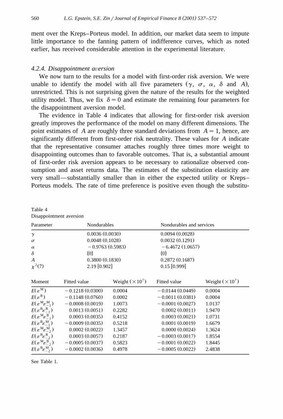
The evidence in Table 4 indicates that allowing for first-order risk aversiongreatly improves the performance of the model on many different dimensions. Thepoint estimates of A are roughly three standard deviations from As1, hence, aresignificantly different from first-order risk neutrality. These values for A indicatethat the representative consumer attaches roughly three times more weight todisappointing outcomes than to favorable outcomes. That is, a substantial amountof first-order risk aversion appears to be necessary to rationalize observed con-sumption and asset returns data. The estimates of the substitution elasticity arevery small—substantially smaller than in either the expected utility or Kreps–Porteus models. The rate of time preference is positive even though the substitu-
Table 4Disappointment aversion
Parameter Nondurables Nondurables and services
Ž . Ž .g 0.0036 0.0030 0.0094 0.0028Ž . Ž .s 0.0048 0.1028 0.0032 0.1291Ž . Ž .a y0.9763 0.5983 y6.4672 1.0657
� 4 � 4d 0 0Ž . Ž .A 0.3800 0.1830 0.2872 0.1687
2Ž . w x w xx 7 2.19 0.902 0.15 0.999
Ž 7 . Ž 7 .Moment Fitted value Weight =10 Fitted value Weight =10MŽ . Ž . Ž .E ´ y0.1218 0.0300 0.0004 y0.0144 0.0449 0.0004BŽ . Ž . Ž .E ´ y0.1148 0.0760 0.0002 y0.0011 0.0381 0.0004M MŽ . Ž . Ž .E ´ ´ y0.0008 0.0019 1.0073 y0.0001 0.0027 1.0137y1B BŽ . Ž . Ž .E ´ ´ 0.0013 0.0051 0.2282 0.0002 0.0011 1.9470y1M BŽ . Ž . Ž .E ´ ´ 0.0003 0.0035 0.4152 0.0003 0.0021 1.0731y1B MŽ . Ž . Ž .E ´ ´ y0.0009 0.0035 0.5218 0.0001 0.0019 1.6679y1M MŽ . Ž . Ž .E ´ ´ 0.0002 0.0022 1.3457 0.0000 0.0024 1.3624y2B BŽ . Ž . Ž .E ´ ´ 0.0003 0.0057 0.2187 y0.0003 0.0017 1.8554y2M BŽ . Ž . Ž .E ´ ´ y0.0005 0.0037 0.5823 y0.0001 0.0022 1.8445y2B MŽ . Ž . Ž .E ´ ´ y0.0002 0.0036 0.4978 y0.0005 0.0022 2.4838y2
See Table 1.
( )L.G. Epstein, S.E. ZinrJournal of Empirical Finance 8 2001 537–572 561
tion elasticity is small. A negative rate of time preference is not needed in thismodel to match the average levels of returns. In other words, the model appears tobe generating sensible results with economically meaningful values of the parame-ters.
The over-identifying restrictions test almost never rejects this model. Thepotential for singularity in a system of moment restrictions is always a concern.However, the matrix in the quadratic form used to construct the x 2 test had a
Ž .substantially larger condition number ratio of the smallest to largest eigenvaluein this case than for any of the other models. It is, therefore, unlikely that the risk
Ž .of a singularity is greater than for any of the other models which typically reject .The estimated moments and their standard errors indicate that this model generatesmoments that are much closer to their theoretical value than any of the otherspecifications. The pattern of fitting stock restrictions more closely than bondrestrictions is no longer present. The mean of each error appears to be receivingapproximately the same weight and the same is true for the autocovariances.Overall, the empirical performance of this model appears to be very good.
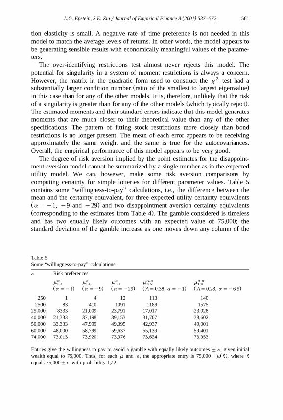
The degree of risk aversion implied by the point estimates for the disappoint-ment aversion model cannot be summarized by a single number as in the expectedutility model. We can, however, make some risk aversion comparisons bycomputing certainty for simple lotteries for different parameter values. Table 5contains some Awillingness-to-payB calculations, i.e., the difference between themean and the certainty equivalent, for three expected utility certainty equivalentsŽ .asy1, y9 and y29 and two disappointment aversion certainty equivalentsŽ .corresponding to the estimates from Table 4 . The gamble considered is timelessand has two equally likely outcomes with an expected value of 75,000; thestandard deviation of the gamble increase as one moves down any column of the
Table 5Some Awillingness-to-payB calculations
´ Risk preferencesa a a A,a A,am m m m mEU EU EU DA DA
Ž . Ž . Ž . Ž . Ž .asy1 asy9 asy29 As0.38, asy1 As0.28, asy6.5
250 1 4 12 113 1402500 83 410 1091 1189 1575
25,000 8333 21,009 23,791 17,017 23,02840,000 21,333 37,198 39,153 31,707 38,60250,000 33,333 47,999 49,395 42,937 49,00160,000 48,000 58,799 59,637 55,139 59,40174,000 73,013 73,920 73,976 73,624 73,953
Entries give the willingness to pay to avoid a gamble with equally likely outcomes "´ , given initialŽ .wealth equal to 75,000. Thus, for each m and ´ , the appropriate entry is 75,000ym x , where x˜ ˜
equals 75,000"´ with probability 1r2.
( )L.G. Epstein, S.E. ZinrJournal of Empirical Finance 8 2001 537–572562
table. From these calculations, we can see that even for a small gamble, theexpected utility model does not differ much from risk neutrality, even for a ‘large’degree of relative risk aversion, while the disappointment aversion model displayssubstantial risk aversion. However, for a range of moderate to large gambles, thedisappointment aversion certainty equivalent corresponding to As0.38 and asy1 exhibits less risk aversion than an expected utility certainty equivalent with a
Ž Ž .‘moderate’ value of relative risk aversion, asy9. See Epstein and Zin 1990.for additional comparisons of risk aversion along these lines.
We note that what constitutes a ‘moderate’ or ‘large’ magnitude for the degreeŽ .of relative risk aversion RRA is not at all clear. While the conventional wisdom
Žhas until recently held that only values of RRA less than 10 are reasonable e.g.,. Ž .Mehra and Prescott, 1985 , Kandel and Stambaugh 1990 have raised serious
doubts about the validity of arguments typically invoked to support this view. Thedisappointment aversion model, of course, is not immune to this debate. Whetheror not one should view the degree of risk aversion embodied in the results in Table4 to be implausibly large is equally unclear. However, it is clear that since ‘large’second-order risk aversion alone still leads to rejections of the theory, it is the‘large’ first-order risk aversion that improves the empirical performance of themodel. Although this property is structural in the context of the representativeagent formulation of this paper, there is some reason to believe that it may bereflecting a feature of the market structure rather than individual preferences. For
Ž .example, Epstein 1991 presents a simple example in which an exogenouslygiven, suboptimal risk-sharing rule leads to community preferences that exhibitfirst-order risk aversion, even though all individuals have standard expectedpreferences. There is also an interesting link between the disappointment aversionmodel and stochastic process switching models, to which we now turn.
4.3. Switching models for consumption and MRS
When consumption growth exhibits stochastic process switching, expectedŽutility models generates more plausible asset-pricing predictions e.g., Cecchetti et
.al., 1989; Kandel and Stambaugh, 1990 . This is similar to the inclusion ofŽso-called Adisaster statesB in the consumption growth process e.g., Reitz, 1988;
.Backus et al., 1989 . We now examine an interesting empirical similarity betweenthese models and the disappointment aversion model.
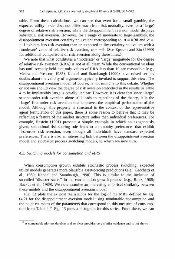
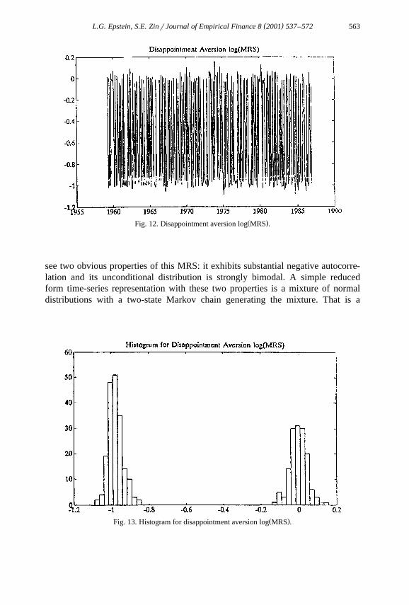
Fig. 12 plots the ex post realizations for the log of the MRS defined by Eq.Ž .4.2 for the disappointment aversion model using nondurable consumption andthe point estimates of the parameters that correspond to this measure of consump-tion from Table 4.11 Fig. 13 plots a histogram for this series. From these, we can
11 A comparable plot nondurables and services provides very similar evidence and is not shown.
( )L.G. Epstein, S.E. ZinrJournal of Empirical Finance 8 2001 537–572 563
Ž .Fig. 12. Disappointment aversion log MRS .
see two obvious properties of this MRS: it exhibits substantial negative autocorre-lation and its unconditional distribution is strongly bimodal. A simple reducedform time-series representation with these two properties is a mixture of normaldistributions with a two-state Markov chain generating the mixture. That is a
Ž .Fig. 13. Histogram for disappointment aversion log MRS .
( )L.G. Epstein, S.E. ZinrJournal of Empirical Finance 8 2001 537–572564
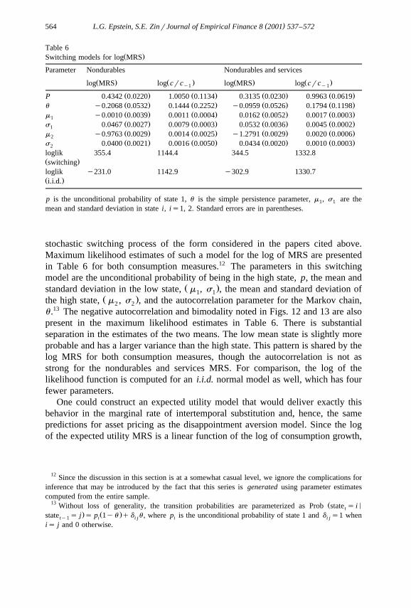
Table 6Ž .Switching models for log MRS
Parameter Nondurables Nondurables and services
Ž . Ž . Ž . Ž .log MRS log crc log MRS log crcy1 y1
Ž . Ž . Ž . Ž .P 0.4342 0.0220 1.0050 0.1134 0.3135 0.0230 0.9963 0.0619Ž . Ž . Ž . Ž .u y0.2068 0.0532 0.1444 0.2252 y0.0959 0.0526 0.1794 0.1198Ž . Ž . Ž . Ž .m y0.0010 0.0039 0.0011 0.0004 0.0162 0.0052 0.0017 0.00031Ž . Ž . Ž . Ž .s 0.0467 0.0027 0.0079 0.0003 0.0532 0.0036 0.0045 0.00021Ž . Ž . Ž . Ž .m y0.9763 0.0029 0.0014 0.0025 y1.2791 0.0029 0.0020 0.00062Ž . Ž . Ž . Ž .s 0.0400 0.0021 0.0016 0.0050 0.0434 0.0020 0.0010 0.00032
loglik 355.4 1144.4 344.5 1332.8Ž .switchingloglik y231.0 1142.9 y302.9 1330.7Ž .i.i.d.
p is the unconditional probability of state 1, u is the simple persistence parameter, m , s are the1 1
mean and standard deviation in state i, is1, 2. Standard errors are in parentheses.
stochastic switching process of the form considered in the papers cited above.Maximum likelihood estimates of such a model for the log of MRS are presentedin Table 6 for both consumption measures.12 The parameters in this switchingmodel are the unconditional probability of being in the high state, p, the mean and
Ž .standard deviation in the low state, m , s , the mean and standard deviation of1 1Ž .the high state, m , s , and the autocorrelation parameter for the Markov chain,2 2
u .13 The negative autocorrelation and bimodality noted in Figs. 12 and 13 are alsopresent in the maximum likelihood estimates in Table 6. There is substantialseparation in the estimates of the two means. The low mean state is slightly moreprobable and has a larger variance than the high state. This pattern is shared by thelog MRS for both consumption measures, though the autocorrelation is not asstrong for the nondurables and services MRS. For comparison, the log of thelikelihood function is computed for an i.i.d. normal model as well, which has fourfewer parameters.
One could construct an expected utility model that would deliver exactly thisbehavior in the marginal rate of intertemporal substitution and, hence, the samepredictions for asset pricing as the disappointment aversion model. Since the logof the expected utility MRS is a linear function of the log of consumption growth,
12 Since the discussion in this section is at a somewhat casual level, we ignore the complications forinference that may be introduced by the fact that this series is generated using parameter estimatescomputed from the entire sample.
13 ŽWithout loss of generality, the transition probabilities are parameterized as Prob state s iNt. Ž .state s j s p 1yu qd u , where p is the unconditional probability of state 1 and d s1 whenty1 i i j i i j
is j and 0 otherwise.
( )L.G. Epstein, S.E. ZinrJournal of Empirical Finance 8 2001 537–572 565
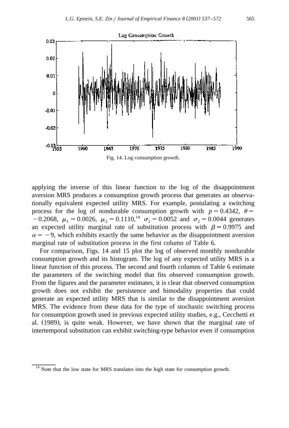
Fig. 14. Log consumption growth.
applying the inverse of this linear function to the log of the disappointmentaversion MRS produces a consumption growth process that generates an observa-tionally equivalent expected utility MRS. For example, postulating a switchingprocess for the log of nondurable consumption growth with ps0.4342, usy0.2068, m s0.0026, m s0.1110,14 s s0.0052 and s s0.0044 generates1 2 1 2
an expected utility marginal rate of substitution process with bs0.9975 andasy9, which exhibits exactly the same behavior as the disappointment aversionmarginal rate of substitution process in the first column of Table 6.
For comparison, Figs. 14 and 15 plot the log of observed monthly nondurableconsumption growth and its histogram. The log of any expected utility MRS is alinear function of this process. The second and fourth columns of Table 6 estimatethe parameters of the switching model that fits observed consumption growth.From the figures and the parameter estimates, it is clear that observed consumptiongrowth does not exhibit the persistence and bimodality properties that couldgenerate an expected utility MRS that is similar to the disappointment aversionMRS. The evidence from these data for the type of stochastic switching processfor consumption growth used in previous expected utility studies, e.g., Cecchetti et
Ž .al. 1989 , is quite weak. However, we have shown that the marginal rate ofintertemporal substitution can exhibit switching-type behavior even if consumption
14 Note that the low state for MRS translates into the high state for consumption growth.
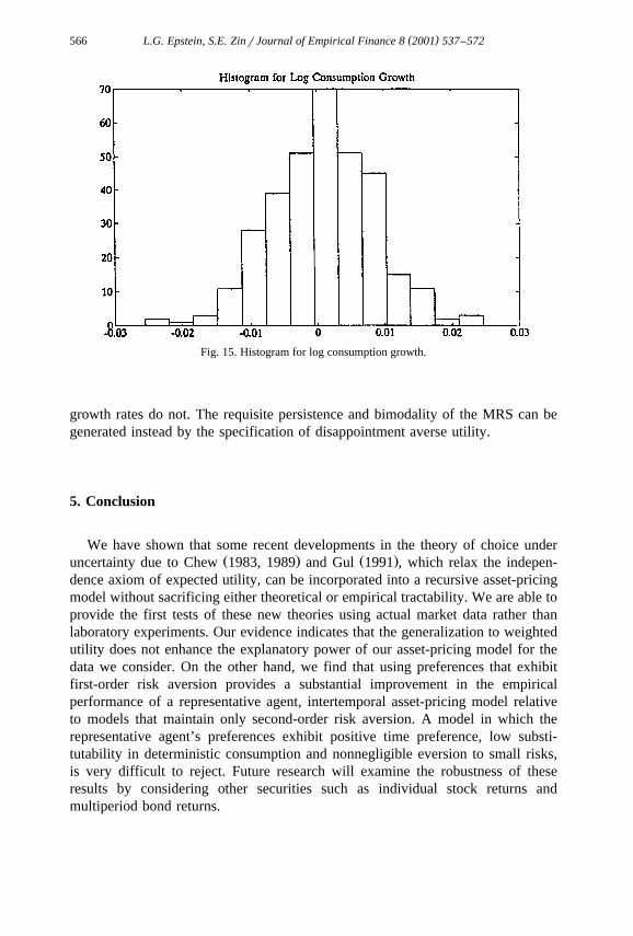
( )L.G. Epstein, S.E. ZinrJournal of Empirical Finance 8 2001 537–572566
Fig. 15. Histogram for log consumption growth.
growth rates do not. The requisite persistence and bimodality of the MRS can begenerated instead by the specification of disappointment averse utility.
5. Conclusion
We have shown that some recent developments in the theory of choice underŽ . Ž .uncertainty due to Chew 1983, 1989 and Gul 1991 , which relax the indepen-
dence axiom of expected utility, can be incorporated into a recursive asset-pricingmodel without sacrificing either theoretical or empirical tractability. We are able toprovide the first tests of these new theories using actual market data rather thanlaboratory experiments. Our evidence indicates that the generalization to weightedutility does not enhance the explanatory power of our asset-pricing model for thedata we consider. On the other hand, we find that using preferences that exhibitfirst-order risk aversion provides a substantial improvement in the empiricalperformance of a representative agent, intertemporal asset-pricing model relativeto models that maintain only second-order risk aversion. A model in which therepresentative agent’s preferences exhibit positive time preference, low substi-tutability in deterministic consumption and nonnegligible eversion to small risks,is very difficult to reject. Future research will examine the robustness of theseresults by considering other securities such as individual stock returns andmultiperiod bond returns.
( )L.G. Epstein, S.E. ZinrJournal of Empirical Finance 8 2001 537–572 567
Acknowledgements
The first author gratefully acknowledges the financial support of the SocialSciences and Humanities Research Council of Canada. We are also indebted toChew Soo Hong, Robert Miller and Fallaw Sowell for valuable discussions. Thispaper is part of NBER’s research program in Financial Markets and MonetaryEconomics. Any opinions expressed are those of the authors and not those of theNational Bureau of Economic Research.
Appendix A
A.1. Properties of mSW
Ž . Ž .Recall the definition Eq. 2.3 of m where f is given by Eqs. 2.4 andSWŽ . XŽ . YŽ .2.5 . Note that f 1 )0 and f 1 -0. Thus, f is strictly increasing and
w x Ž . Žconcave on an interval a, b containing 1. Note also that f 1 s0. Under Eq.Ž . .2.7 , the preceding is true for any positive numbers a and b.
w xLet F have support in a, ` . Then:
f xra d F x G f 1 d F x s0.Ž . Ž . Ž . Ž .H HOn the other hand, if F has finite mean m, then by Jensen’s inequality:
f xrm d F x Ff 1 s0.Ž . Ž . Ž .HŽ . Ž . Ž . Ž .Thus, there exists a unique l such that Hf xrl d F x s0. We define m FSW
sl.Ž . Ž .Properties 2.1 and 2.2 are immediate. Consistency with first-degree stochas-
tic dominance and risk aversion follows from the monotonicity and concavity off. For example, if G is a mean preserving spread of F, then:
f xrm F d F xŽ . Ž .Ž .H SW
s0s f xrm G dG x F f xrm G d F xŽ . Ž . Ž . Ž .Ž . Ž .H HSW SW
´m F Gm G .Ž . Ž .SW SW
A.2. DeriÕation of the Euler equations
Ž . Ž .Turn to the derivation of the Euler Eq. 3.4 . It follows from Eq. 2.3 andŽ . )Epstein and Zin 1989, pp. 957–958 that the optimal portfolio share vector v t
solves:ry1 rrŽ .1rr 1yr rr TŽ .˜max E f b M c rc v r , A.1Ž .Ž .˜ ˜v t tq1 tq1 t tq1
( )L.G. Epstein, S.E. ZinrJournal of Empirical Finance 8 2001 537–572568
˜ )Twhere r is the vector of gross real returns, M sv r , the return to the˜ ˜tq1 tq1 t tq1Ž . �market porfolio, and where vs v , . . . , v varies over the simplex v: v G01 N i
4for all i and Ýv s1 . We will show that, under additional assumptions, theiŽ . )objective function in Eq. A.1 is differentiable at v and the associatedt
Ž .first-order conditions are given by Eq. 3.4 . The existence of an interior optimumis assumed.
Ž .Recall the definition Eq. 3.6 of z and define:tq1
x d x ay1 ra , a/0,Ž .g x sŽ .
d½ x log x , as0.Ž .
Ž Ž ..The optimization problem Eq. A.1 can be written:
max g z My1 vTr d FŽ .Hv tq1 tq1 tq1 t
q Ay1 g z My1 vTr d F ,Ž . Ž .H tq1 tq1 tq1 ty1 Tz M v r G1� 4tq1 tq1 tq1
where F is the appropriate conditional cdf. Since g is differentiable, the onlyt
potential difficulty arises because the domain of the second integral depends uponv and because A/1, in general.
Define:
c v s g z d F . A.2Ž . Ž . Ž .H tq1 ty1 Tz M v r G1� 4tq1 tq1 tq1
When there is positive probability associated with z s1, c can fail to betq1
differentiable at vsv ). However, under Assumptions 1 and 2, c is differen-t
tiable there and:
c v ) yc v ) s0, i , js1, . . . , N. A.3Ž .Ž . Ž .i t j t
Ž . Ž .It then follows that Eq. 3.4 represents the first-order conditions for Eq. A.1 .
Assumption 1. For each information set at time t, the conditional distribution ofr has compact support in the positive orthant.tq1
Assumption 2. For each information set at t, there exists an ´)0 such that:
y1sup ´ Prob z : 1y´-z -1q´ -`.� 4˜ ˜Ž .0- ´- ´ t tq1 tq1
A necessary condition for Assumption 2 is that the conditional probability thatz s1 be zero. A sufficient condition is that z have bounded conditional˜ ˜tq1 tq1
density function.
( )L.G. Epstein, S.E. ZinrJournal of Empirical Finance 8 2001 537–572 569
Ž .One can apply elementary arguments and the fact that g 1 s0 to the differ-Ž .ence quotient corresponding to Eq. A.3 to prove the latter. Details are omitted.
A.3. Asymptotic properties of the GMM estimator
Turn now to the asymptotic properties of the GMM estimator when A/1. Inthis case, the objective function is not differentiable. We, therefore, employ the
Ž . Ž .results in Andrews 1989a,b to show how the arguments in Hansen 1982 can bemodified to deal with this nonstandard situation. The application of these results toour problem is straightforward so we simply outline the steps involved in deriving
Ž .asymptotic properties for the GMM estimator. Note that unlike Andrews 1989a,b ,we do not have the added complication of infinite dimensional nuisance parameterestimation; all of the parameters in our model are finite dimensional.
Ž . y1 T ŽFor simplicity, consider first the just-identified case. Let fT b 'T Ý f x ,ts1 t. Ž .b be the sample analogue for a sample of size T of the population orthogonality
Ž .restrictions based on Eq. 4.7 , where x is the vector of variables and b is thetŽ .vector of parameters. The GMM estimator, b , is defined such that f b s0T T T
Ž .and the true value of the parameter vector, b , is such that Ef b s0. If a0 T 0Ž .uniform law of large numbers holds for f b and if b is identified, then aT 0
Ž ..standard proof e.g., Hansen, 1982; or Andrews, 1989a, Theorem 1.1 of theŽ .consistency of b can be constructed when Ef b is continuous. The continuityT T
of this expectation follows from the discussion in Appendix A2 and will beassumed from here on.
Ž . Ž .Since the functions defined in Eqs. 4.4 and 4.5 are not differentiable in theŽ .parameters of the model, the mean value expansion of f b at b , which isT T 0
typically used to establish asymptotic normality for the GMM estimator, does notŽ .necessarily exist. We can, however, expand Ef b at b since this function isT 0 T
differentiable. This expansion has the form:
EEf bŽ .T TEf b sEf b y b yb .Ž . Ž . Ž .T 0 T T T 0
Eb
1r2 Ž .where b is between b and b . This implies that T b yb is asymptoti-T T 0 T 01r2 Ž . Ž .cally normal distributed if T Ef b has this property, since Ef b equals 0T T T 0
by definition. Note the difference in this result from the standard argument which1r2 Ž . 1r2 Ž .says that T b yb is asymptotically normally distributed if T f b hasT 0 T 0
this property.Ž . 1r2 w Ž . Ž .xDefine the empirical process, Õ b 'T f b yEf b . If this processT T T
Ž .has the property of stochastic equicontinuity as defined in Andrews, 1989b atŽ .the b , and if b is consistent for b , then Õ b is asymptotically equivalent to0 T 0 T T
Ž . 1r2 Ž .Õ b . This in turn implies that T Ef b is asymptotically equivalent toT 0 T T1r2 Ž . Ž . Ž .yT f b , since both Ef b and f b are zero by definition. When aT 0 T 0 T T
( )L.G. Epstein, S.E. ZinrJournal of Empirical Finance 8 2001 537–572570
1r2 Ž .central limit theorem holds for T f b as in the standard case, it follows thatT 01r2 Ž .T f b yb is asymptotically normally distributed with covariance matrix:T T 0
y1 y1EEf b EEf bŽ . Ž .T 0 T 01r2Var T f b .Ž .T 0
Eb Eb
An estimator of the matrix of derivatives in this expression can be constructedŽ .using a finite difference of the sample average as in Pakes and Pollard, 1989
evaluated at a consistent estimator for b , provided the finite difference converges0
to zero at an appropriate rate as the sample size gets large. The variance of theorthogonality conditions in the middle of this expression can be consistently
Ž . Ž .Testimated in the standard way by using the sample average of f x , b f x , b ,t t
evaluated at a consistent estimator for b .0
When the model is over-identified, b is defined as the minimizer of theTŽ .T Ž .quadratic form f b W f b , where W is a positive definite matrix that canT T T T
depend on the sample size and has a probability limit of W. As in the just-identi-Ž .fied case, asymptotic normality follows from an expansion of Ef b around b .T 0 T
wŽ Ž .. xTPremultiply both sides of this expansion by EEf b rEb W. It follows thatT 0wŽ Ž .. xT 1r2 Ž . Ž .when EEf b rEb WT f b is o 1 and the stochastic equicontinuityT 0 T T p
1r2Ž .condition holds, T b yb is asymptotically normally distributed with covari-T 0
ance matrix:
y1 y1T T 1r2 TD WD D W Var T f b WD D WD ,Ž .Ž . Ž .Ž .0 0 0 T 0 0 0 0
wŽ Ž .. x y1where D s EEf b rEb . When W s V where V is equal to0 T 0w 1r2 xy1Var T f b , the asymptotic covariance matrix of the GMM estimator isT 0
Ž T y1 .y1D V D . This defines an efficient estimator in the sense that this covariance0 0
matrix differs from the covariance matrix of an estimator defined for an arbitrarychoice of weighting matrix, W , by a positive semidefinite matrix. Further, forT
Ž .T y1 Ž . 2this efficient estimator, Tf b V f b has a limiting x distribution withT T T T
degrees of freedom equal to the number of restrictions less the number ofestimated parameters. Note that this result differs from the just-identified case by
wŽ Ž .. xT 1r2 Ž .requiring that EEf b rEb WT f b converge to zero in probability asT 0 T T
the sample size gets arbitrarily large. When the objective function is differentiable,the analogous condition to this follows from the necessary conditions for theoptimization problem that defines the estimator. Alternatively, one can think of the
Žover-identified model as corresponding to a particular just-identified model as in. Ž .Hansen, 1982 , by defining it as the solution to a f b s0, where a hasT T T T
column dimension equal to the number of orthogonality restrictions and rowdimension equal to the number of parameters, i.e., the estimator sets a particularlinear combination of the orthogonality restrictions equal to zero. In the differen-tiable case, a can be thought of as defining the first-order conditions. In theT
wŽ Ž .. xTnondifferentiable case, when a converges to EEf b rEb W, the asymptoticT T 0
results discussed above will hold without any additional assumptions. Therefore,
( )L.G. Epstein, S.E. ZinrJournal of Empirical Finance 8 2001 537–572 571
constructing a just-identified GMM estimator for the linear combinations of thewŽ Ž .. xTorthogonality restrictions given by a consistent estimator of EEf b rEb WT 0
results in an estimator that is asymptotically equivalent to the estimator based onwŽ Ž ..the minimization of the quadratic form and the requirement that EEf b rT 0
xT 1r2 Ž . Ž .Eb WT f b so 1 .T T p
The results discussed above rely on the stochastic equicontinuity of theempirical process. Sufficient conditions for this in a time-series context that can be
Ž .applied to our model are given in Andrews 1989b . Note that the functions thatŽwe deal with involve his type I and type III functions indicator functions and
.power functions .
References
Andrews, D.W.K., 1989. Asymptotics for semiparametric econometric models: Estimation, Cowlesdiscussion paper no. 908, Yale University.
Andrews, D.W.K., 1989. Asymptotics for semiparametic econometric models: II. Stochastic equiconti-nuity, Cowles discussion paper no. 909, Yale University.
Arrow, K.J., 1965. The theory of risk aversion. Aspects of the Theory of Risk Bearing. Yrjo JahnsonSaatio, Helsinki, Chap. 2.
Backus, D.K., 1989. Risk premiums in the term structure: evidence from artificial economies. Journalof Monetary Economics 24, 371–399.
Camerer, C.F., 1989a. An experimental test of several generalized utility theories. Journal of Risk andUncertainty 2, 61–104.
Camerer, C.F., 1989b. Recent of generalizations of expected utility theory, mimeo. University ofPennsylvania, Philadelphia.
Cecchetti, S.G., Lam, P., Mark, N.C., 1989. The equity premium and the risk free rate: matching themoments, mimeo. Ohio State University, Columbus.
Chew, S.H., 1983. A generalization of the quasilinear mean with applications to the measurement ofincome inequality and decision theory resolving the Allais paradox. Econometrica 51, 1065–1092.
Chew, S.H., 1989. Axiomatic utility theories with the betweenness property. Annals of OperationsResearch 19, 273–298.
Chew, S.H., Waller, W.S., 1986. Empirical tests of weighted utility theory. Journal of MathematicalPsychology 30, 55–72.
Conlisk, J., 1989. Three variants on the Allais example. American Economic Review 79, 392–407.Duffie, D., Epstein, L.G., 1990. Stochastic differential utility and asset pricing, mimeo. Stanford
University, Stanford.Epstein, L.G., 1991. Behaviour under risk: recent development in theory and applications. In: Laffont,
Ž .J.J. Ed. , Forthcoming in Advances in Economic Theory. Cambridge Univ. Press, Cambridge.Epstein, L.G., Zin, S.E., 1989. Substitution, risk aversion and the temporal behavior of consumption
and asset returns: a theoretical framework. Econometrica 57, 937–969.Epstein, L.G., Zin, S.E., 1990. ‘First-order’ risk aversion and the equity premium puzzle. Journal of
Monetary Economics 26, 387–407.Epstein, L.G., Zin, S.E., 1991. Substitution, risk aversion and the temporal behavior of consumption
and asset returns: an empirical analysis. Journal of Political Economy 99, 263–286.Fishburn, P.C., 1983. Transitive measurable utility. Journal of Economic Theory 31, 293–317.Gallant, R., Hansen, L.P., Tauchen, G., 1991. Using conditional moments of asset payoffs to infer the
volatility of intertemporal marginal rates of substitution. Journal of Econometrics 45, 141–180.
( )L.G. Epstein, S.E. ZinrJournal of Empirical Finance 8 2001 537–572572
Ž .Gul, F., 1991. A theory of disappointment aversion. Econometrica 59 3 , 667–689.Hansen, L.P., 1982. Large sample properties of generalized method of moments estimators. Economet-
rica 50, 1029–1054.Hansen, L.P., Jagannathan, R., 1991. Implications of security market data for models of dynamic
economies. Journal of Political Economy 99, 225–262.Hansen, L.P., Richard, S., 1987. The role of conditioning information in deducing testable restrictions
implied by dynamic asset pricing models. Econometrica 55, 587–613.Hansen, L.P., Singleton, K.J., 1982. Generalized instrumental variables estimation of nonlinear rational
expectations models. Econometrica 50, 1269–1286.Hansen, L.P., Singleton, K.J., 1983. Stochastic consumption, risk aversion and the temporal behavior
of asset returns. Journal of Political Economy 91, 249–265.Harrison, G., 1990. Expected utility theory and the experimentalists, working paper B-90-04. Univer-
sity of South Carolina.Kahneman, D., Tversky, A., 1979. Prospect theory: an analysis of choice under risk. Econometrica 47,
263–291.Kandel, S., Stambaugh, R.F., 1990. Modelling expected stock returns for long and short horizons,
mimeo. University of Pennsylvania, Philadelphia.Kandel, S., Stambaugh, R.F., 1990. Asset returns and intertemporal preferences, NBER working paper
no. 3633.Kreps, D.M., Porteus, E.L., 1978. Temporal resolution of uncertainty and dynamic choice theory.
Econometrica 46, 185–200.Machina, M.J., 1982. ‘Expected utility’ analysis without the independence axiom. Econometrica 50,
277–323.Mehra, R., Prescott, E., 1985. The equity premium: a puzzle. Journal of Monetary Economics 15,
145–161.Pakes, A., Pollard, D., 1989. Simulation and symptotics of optimization. Econometrica 57, 1027–1057.Quiggin, J.C., 1982. A theory of anticipated utility. Journal of Economic Behavior and Organization 3,
323–343.Reitz, T., 1988. The equity premium: a solution. Journal of Monetary Economics 22, 117–131.Segal, U., 1989. Axiomatic representation of expected utility with rank-dependent probabilities. Annals
of Operations Research 19, 359–373.Segal, U., Spivak, A., 1990. ‘First-order’ versus ‘second-order’ risk aversion. Journal of Economic
Theory 51, 111–125.Singleton, K.J., 1987. Specification and estimation of intertemporal asset pricing models. In: Friedman,
Ž .B., Hahn, F. Eds. , Handbook in Monetary Economics.Yaari, M.E., 1987. The dual theory of choice under risk. Econometrica 55, 95–115.