Finance and Economics Discussion SeriesDivisions of Research & Statistics and Monetary Affairs

Federal Reserve Board, Washington, D.C.

The Income-Achievement Gap and Adult Outcome Inequality

Eric R. Nielsen

2015-041

Please cite this paper as:Eric R. Nielsen (2015). “The Income-Achievement Gap and Adult Outcome Inequality,”Finance and Economics Discussion Series 2015-041. Washington: Board of Governors of theFederal Reserve System, http://dx.doi.org/10.17016/FEDS.2015.041.

NOTE: Staff working papers in the Finance and Economics Discussion Series (FEDS) are preliminarymaterials circulated to stimulate discussion and critical comment. The analysis and conclusions set forthare those of the authors and do not indicate concurrence by other members of the research staff or theBoard of Governors. References in publications to the Finance and Economics Discussion Series (other thanacknowledgement) should be cleared with the author(s) to protect the tentative character of these papers.

THE INCOME-ACHIEVEMENT GAP AND ADULT OUTCOMEINEQUALITY*

ERIC R. NIELSEN

THE FEDERAL RESERVE BOARD

Abstract. This paper discusses various methods for assessing group differences in

academic achievement using only the ordinal content of achievement test scores. Re-

searchers and policymakers frequently draw conclusions about achievement differences

between various populations using methods that rely on the cardinal comparability

of test scores. This paper shows that such methods can lead to erroneous conclu-

sions in an important application: measuring changes over time in the achievement

gap between youth from high- and low-income households. Commonly-employed, car-

dinal methods suggest that this “income-achievement gap” did not change between

the National Longitudinal Surveys of Youth (NLSY) 1979 and 1997 surveys. In con-

trast, ordinal methods show that this gap narrowed substantially for reading achieve-

ment and may have narrowed for math achievement as well. In fact, any weighting

scheme that places more value on higher test scores must conclude that the read-

ing income-achievement gap decreased between these two surveys. The situation for

math achievement is more complex, but low-income students in the middle and high

deciles of the low-income math achievement distribution unambiguously gained rela-

tive to their high-income peers. Furthermore, an anchoring exercise suggests that the

narrowing of the income-achievement gap corresponds to an economically significant

convergence in lifetime labor wealth and school completion rates for youth from high-

and low-income backgrounds. JEL Codes: I24, I21, J24, C18, C14.

Date: May 14, 2015.*I thank Derek Neal, Gary Becker, Ali Hortaçsu, James Heckman, Sandy Black, Armin Rick, andseminar participants at the University of Chicago, Federal Reserve Board, and the DC EducationWorking Group. The views and opinions expressed in this paper are solely those of the author and donot reflect those of the Board of Governors or the Federal Reserve System.Contact: Division of Research and Statistics, Board of Governors of the Federal Reserve System, MailStop 97, 20th and C Street NW, Washington, D.C. 20551. eric.r.nielsen@frb.gov. (202) 872-7591.

1

1. Introduction

Economists and policymakers frequently use standardized test score data to measure

group differences in academic achievement. For example, researchers use achievement

test scores to measure changes in the black-white achievement gap over time, to assess

school and teacher quality, and to quantify the importance of class size and other school

inputs for student achievement. A fundamental question in all of these applications is

how best to use test score data to measure student achievement. The typical methods

employed in education economics provide a deeply inadequate answer to this question.

In almost all empirical work, researchers first normalize test scores to have a mean

of zero and a standard deviation of one within each year/age cohort and then compare

these normalized scores (or “z-scores”) across different cohorts using standard statistical

techniques, such as mean differences or regression. This approach makes two very strong

assumptions on the normalized test scores. First, it assumes that the normalized test

scale has a constant interpretation throughout the range of scores, so that a score change

of x represents the same change in achievement at all starting locations in the test scale.

Second, it assumes that a given z-score has a fixed interpretation across all cohorts.

Neither of these assumptions is well justified by either economic or psychometric theory,

and if either fails, standard methods may produce biased estimates. It is even possible

for these methods to misidentify the sign of the achievement change.

In recent work, Reardon (2011) uses such standard methods to argue that the income-

achievement gap has increased markedly over the last several decades. This dramatic

finding has received substantial press coverage and has been cited frequently in a grow-

ing body of academic research.1 This excitment is understandable, as the income-

achievement gap is an important driver of intergenerational mobility and adult outcome

inequality. Unfortunately, Reardon’s conclusions rely very heavily on the cardinal com-

parability of test scores, both in the cross section and over time.

1In the popular press, see Garland (2013) and Tevernise (2012), among others. In the academicliterature, Corak (2013), Jerrim and Vignoles (2013), and many others cite Reardon’s work.

2

This paper makes two important contributions, one methodological and the other

empirical. On the methodological side, I introduce several ordinal measures of achieve-

ment inequality that are not sensitive to the scale of test scores. I show that there are

precise, testable conditions under which these ordinal measures unambiguously identify

a decrease in achievement inequality. My method has two key components. First, I use

test scores that have been “crosswalked” to ensure that a given score corresponds to

the same underlying level of achievement regardless of the cohort. Second, I compute

achievement gaps using only the rank order of students in the test score distributions.

Empirically, I reexamine Reardon’s findings on the income-achievement gap using these

ordinal methods and find compelling evidence in the NLSY79 and NLSY97 surveys that

the income-achievement gap narrowed substantially between 1980 and 1997.2 This re-

sult stands in sharp contrast to Reardon, who finds no significant change using the

same data.

In particular, I estimate Cliff’s δ, an easy-to compute ordinal statistic that measures

the degree of overlap between two distributions. Estimates of Cliff’s δ uniformly sug-

gest that there was a large, statistically significant decrease in the income-achievement

gap between 1980 and 1997. These estimates are robust to income and test score mea-

surement error, as well as to various methods for adjusting income to reflect household

size and composition. I also test a number of first-order stochastic dominance (FOSD)

relationships in the crosswalked test score data. These tests allow me to make a very

strong claim for reading achievement: any weighting scheme that places greater weight

on higher scores would necessarily measure a smaller achievement gap in 1997 than

in 1980. This conclusion follows because the low-income achievement distribution in

1997 is unambiguously higher than it was in 1980, while the high-income achievement

distribution is unambiguously lower. I cannot make such a strong claim about math

achievement because low-achieving low-income students suffered an adverse shift in

their achievement, while high-achieving low-income students improved unambiguously.

2The NLSY79 provides achievement data for 1980 while the NLSY97 provides data from 1997.3

Nonetheless, any weighting scheme that does not place too much emphasis on the bot-

tom of the achievement distribution would find a smaller math achievement gap in 1997

than in 1980.

Finally, to assess whether these ordinal shifts are economically significant, I use the

NLSY79 to anchor test scores on various later-life outcomes. In particular, I use the

NLSY79 to estimate a set of skill prices that I then use to translate ordinal test score

shifts into economically interpretable units. The results of this anchoring exercise sug-

gest that the achievement test shifts that I document correspond to economically large

shifts in both lifetime labor wealth and school completion rates. Using NLSY79 skill

prices, the decrease in the reading achievement gap between high- and low-income youth

corresponds to a narrowing of the lifetime earnings gap of between $50,000 and $70,000

in present discounted value and a decrease in the high school and college completion

gaps of between 0.05 and 0.07 probability units.

My findings should give researchers who use standard methods pause. Ordinal meth-

ods disagree with traditional cardinal approaches in at least one important setting, and

other findings that use standard methods may be similarly fragile. Ordinal methods

are prima facie more credible, as the conditions needed for them to provide valid infer-

ence are substantially weaker than those required by cardinal methods. When possible,

researchers should use methods that do not rely on the scale of achievement test scores.

The ordinal techniques that I develop in this paper apply to any situation in which

a researcher wishes to use test score data to assess group differences in achievement;

nothing about the analysis assumes that time is the relevant dimension for comparison.

For example, the methods in this paper could be used to compare black-white achieve-

ment inequality in the American South versus the North at a given point in time, or the

achievement of suburban students versus urban students across different metropolitan

areas.

The rest of this paper is organized as follows. Section 2 reviews the literature on using

test scores to assess group achievement differences. Section 3 describes the NLSY data.

Sections 4 and 5 discuss various ordinal estimates of income-achievement gap changes,

4

while Sections 6 and 7 show how to reach even stronger conclusions if crosswalked test

scores are available. Section 8 presents the anchoring analysis. Section 9 discusses the

relationship between my empirical results and the literature on differential investments

in children by parental income class. Section 10 concludes. Appendix A contains proofs

and additional econometric details. Appendices B-C contain all of the empirical results.

2. Literature Review

Recent research by Reardon (2011) argues that the difference in academic achieve-

ment between high-income and low-income students has widened tremendously over

the last half century. Reardon defines the income-achievement gap as the difference in

average academic achievement, measured in z-scores, between students from families

at the 90th percentile and 10th percentile of the household income distribution. He

estimates that this gap is 30 to 40 percent larger for those students born in 2001 than

those born three decades earlier. His regression-based method assumes that the z-scores

are cardinally comparable, both in the cross section and over time.3

My research does not address Reardon’s larger thesis, as I study a much shorter

time period and do not use the full complement of surveys that he employs. The large

increases that Reardon documents come from cross-sectional income-achievement gaps

estimated using surveys other than the NLSY79 and NLSY97. It is possible that my

methods would also find an increasing income-achievement gap with these alternate

data. However, Reardon does use both NLSY surveys in his analysis, and he calculates

a negligible change in the income-achievement gap with these data.

The literature studying changes in achievement gaps over time focuses mostly on

black-white disparities estimated assuming the cardinal comparability of z-scores. For

example, Fryer and Levitt (2004, 2006) study the evolution of the black-white achieve-

ment gap in the first few years of school by comparing standardized test scores.4 Neal

(2006) uses standardized test scores for much of his discussion, yet he also recognizes

3The online appendix contains an exhaustive description of his method.4Other papers in this literature that assume the cardinal comparability of standardized test scoresinclude Clotfelter et al. (2009), Duncan and Magnuson (2006), and Hanushek and Rivkin (2006).

5

that “[a]chievement has no natural units,” and so he also compares percentile rankings

between black and white test takers. This procedure is related to the one I employ,

although he does not conduct inference using ordinal methods.

A number of authors in economics and psychometrics have focused on the sensitivity

of standard statistical approaches to the arbitrary choice of test scale. Lang (2010)

and Cascio and Staiger (2012) argue that standard treatment effects and value-added

estimates are sensitive to arbitrary scaling decisions. In a 2008 working paper, Reardon

(2007) shows that black-white achievement gap estimates are sensitive to the choice of

test scale, while Bond and Lang (2013) show that order-preserving transformations of

achievement test scores can dramatically effect the estimated evolution of the black-

white achievement gap from kindergarten through third grade.5 Stevens (1946) argues

that most psychometric scales are inherently ordinal. Lord (1975) shows that IRT scale

scores from 2- or 3-parameter logistic models are ordinal in the sense that there are

infinitely many rescalings of these scores that will fit any test data equally well.

Cunha et al. (2010), Cunha and Heckman (2008), and many others create inter-

pretable test scales by anchoring scores to later-life, economically meaningful outcomes.

This approach offers an appealing solution to the arbitrariness of achievement test

scales. However, anchoring has a number of significant downsides. Most importantly,

anchoring requires data on outcomes years or even decades after the test date in order

to accurately measure lifetime differences between test subjects. For many pressing

questions, waiting 20 to 30 years for an answer is not a viable option. In addition,

estimates based on anchored scores may be sensitive to the particular outcome chosen

as the anchor and to the functional forms used to implement the anchoring procedure.

Despite these shortcomings, I augment my ordinal estimates by anchoring test scores

on school completion and labor market earnings in Section 8.

5In extreme cases, they find that such transformations can actually reverse the estimated growth inthe gap. The online appendix presents a simple, parametric example in which it is always possible tofind a rescaling such that the estimated gap change calculated using z-scores has the opposite sign asthe true gap change.

6

3. Data

I use the NLSY79 and NLSY97 surveys for all of my analysis. These are high-

quality, nationally representative surveys of young adults that contain detailed family

background and achievement test score data. Both surveys follow respondents through-

out their adult lives, making the anchoring analysis of Section 8 possible. I restrict my

attention to the NLSY surveys simply because they are designed to be comparable to

each other. Other data sources have income and achievement measures that do not

map easily across surveys, adding an additional layer of complexity and uncertainty to

the analysis.

The NLSY79 and NLSY97 collect comprehensive family income information for each

respondent. In my empirical work, I define family income as the sum of all sources of

income for all household members in the base year of each survey.6 As a robustness

check, I rerun the analysis using the average household income in a three-year window

around the base year of the survey and obtain qualitatively similar results.

NLSY respondents took the Armed Services Vocational Aptitude Battery (ASVAB)

near the start of each survey. I use a subset of the ASVAB known as the Armed Forces

Qualifying Test (AFQT), along with its math and reading subsections, as my measures

of academic achievement.7 The ASVAB test format changed between the NLSY79 and

the NLSY97. For reasons that I will explain in Section 6, I would like the achievement

test scores I use to maintain a constant relationship over time between the test score

and the underlying level of achievement. To this end, I make use of a crosswalk created

by Segall (1997) based on a sample of test takers who were randomly assigned to the

two versions of the ASVAB.8

6This definition includes income earned by the respondent herself, in addition to the income earnedby her parents. Since the respondents I study are less than 18 years old, their share of total householdincome is usually negligible. Subsetting on respondents positively identified in the data as beingdependent on their parents has a very minor effect on the ordinal estimates.7The definition of the AFQT changed in 1989; throughout, I will use the current, post-1989 definition.Using the old definition, I estimate somewhat larger and more statistically-significant decreases in themath income-achievement gap.8The NLSY79 test is pencil and paper (P&P) while the NLSY97 test follows a computer adaptivedesign (CAD). The crosswalk is courtesy of Altonji et al. (2011) and is available at the followingurl: http://www.econ.yale.edu/~fl88/data.html. The crosswalk contains a percentile-mapped1980-equivalent score for each component of the CAD ASVAB for each respondent in the NLSY97.

7

I restrict my analysis to respondents who were between the ages of 15 and 17 when

they took the ASVAB. I select this age range for two reasons. First, the two NLSY

surveys have very different age distributions, yet both have large numbers of respondents

in this age range. Focusing on this age group therefore reduces the importance of age

standardization in my empirical work. My results do not change qualitatively if I eschew

age-standardization entirely and instead restrict my analysis to 16-year-old test takers.9

Second, respondents in this age range are just on the cusp of becoming independent

adults. Test scores for such students provide a measure of the cumulative effect of

parental income on achievement through high school.

4. Percentile-Percentile Curves

This section uses percentile-percentile curves (PPCs) to document shifts in the income-

achievement gap between the NLSY79 and the NLSY97. Let L and H denote youth

from low- and high-income households, respectively. The PPC for L relative to H

simply plots the percentiles of the group-L scores in the distribution of group-L scores

against the percentiles of the group-L scores in the distribution of the group-H scores.

Formally, let FL and FH be the cumulative distribution functions (cdfs) for low- and

high-income students. The PPC for L relative to H is given by (pi, qi) i ∈ L, where

pi = FL(si) and qi = FH(si).10 The PPC summarizes how the low-income scores com-

pare to the high-income scores. If the scores in L tend to be lower than the scores in H,

the corresponding PPC will lie below the 45-degree line, since the pth percentile in the

group-L score distribution will correspond to the qth < pth percentile in the group-H

score distribution. The further below the 45-degree line the PPC is, the more the scores

in H dominate those in L.

Comparing PPCs across different surveys allows one to assess changes in the per-

formance of low-income compared to high-income youth. Shifts in the PPCs closer

Creating a 1980-equivalent AFQT score by adding these cross-walked subscores together is not strictlyvalid because it ignores the covariance structure of the different ASVAB components. However, Segall(1999) reports that the AFQT scores resulting from such a procedure are virtually identical to thoseobtained by crosswalking the AFQT scores directly.9The online appendix shows the main ordinal estimates calculated separately for each age.10In practice, these percentiles must be estimated by their obvious sample analogues.

8

to or further from the 45-degree line indicate decreasing or increasing differences, re-

spectively, in the score distributions between the two groups. Only relative changes

in test scores between groups L and H are detectable in the PPCs; if both groups are

experiencing secular increases (or decreases) in their test scores, the curves will show no

change. The empirical PPCs created using income in the NLSY surveys look very much

like Lorenz curves. This is no accident, as the definition of a PPC is very similar to the

definition of a Lorenz curve. Since high-income test scores always dominate low-income

test scores in both NLSY surveys, the PPCs I calculate will all be below the 45-degree

line. However, unlike Lorenz curves, this is not true by construction.11

Figure I in Appendix C displays the math, reading, and AFQT PPCs for the bottom

versus the top income quintiles in both NLSY surveys. The large income-achievement

gap in both surveys is clear from the great distance between all of the PPCs and the

45-degree line. For example, the median reading score in the high-income distribution

of the NLSY79 corresponds roughly to the 90th percentile in the low-income score

distribution.

The reading and AFQT PPCs for 1997 lie uniformly closer to the 45-degree line than

those for 1980. This indicates that the score distributions for high- and low-income

students are more similar to each other in the NLSY97 than in the NLSY79. The shifts

are quite large in magnitude. In the 1980 data, the 60th percentile in the low-income

reading distribution corresponds roughly to the 13th percentile in the high-income dis-

tribution. By 1997, the same point in the low-income distribution corresponds to the

18th percentile in the high-income distribution. The NLSY97 math PPC also lies above

the PPC for 1980, but the two curves coincide almost perfectly for low-income score

percentiles below 50. The convergence in the math score distributions is smaller and

less uniform than the convergence in the reading and AFQT distributions.

Figure II displays black-white achievement inequality by designating white respon-

dents as the H group and black respondents as the L group. Both curves are very

11There is also no constraint that the curves start at (0,0) and end at (1,1). These will be the endpointsonly if both groups have support on the same range of test scores. Furthermore, PPCs may intersectthe 45-degree line any number of times.

9

far below the 45-degree line, indicating that there is substantial black-white achieve-

ment inequality in both surveys. Furthermore, the 1997 curve is always above the 1980

curve, which suggests that the black and white test score distributions became more

similar between the two NLSY surveys. This result is consistent with the findings on

black-white achievement convergence in Altonji et al. (2011) and Neal (2006).

The narrowing of the black-white gap over this time period is a strong force push-

ing against a widening income-achievement gap. Since black students tend to come

from more economically-disadvantaged families than white students, their relative im-

provement implies that a large subpopulation of low-income families gained relative

to wealthier white families.12 Low-income white students would have to have fallen

much farther behind their wealthier white peers in order for the change in the overall

income-achievement gap to have been flat or positive.

PPCs calculated using data restricted by race and sex show shifts in the income-

achievement gap separately for various demographic subgroups. The PPCs restricted

to white respondents suggest that the income-achievement gap for whites narrowed be-

tween the two surveys, while the PPCs for black respondents suggest that the income-

achievement gap for black youth may have widened. This conclusion for black re-

spondents is sensitive to whether or not income is adjusted for household size and

composition. Similarly, the PPCs for women show little evidence of a shift in the

income-achievement gap, while the PPCs for men indicate a sharp decrease in achieve-

ment inequality between 1980 and 1997.13

5. Cliff’s δ

5.1. Estimates and Discussion. The PPCs provide suggestive evidence that the

income-achievement gap narrowed between 1980 and 1997, but they do not readily

12For example, the black respondents in my NLSY79 sample have household incomes of $26,000 ayear, versus $47,000 for whites. In 1997 the means shifted to $30,000 and $61,000, respectively. In theNLSY79, 37% of the bottom income quintile is black, compared just 3.6% of the top income quintile.In the NLSY97, 29% of the bottom income quintile is black, compared to 7% in the top quintile.13PPCs in which the H category is all men and the L category is all women indicate that there wasvery little change in male-female achievement inequality between the two surveys. Please refer to theonline appendix for the PPCs broken down by race and sex.

10

admit formal hypothesis testing. Tests of first-order stochastic dominance are feasible,

but the resulting test statistics are not interpretable as effect sizes.14 I therefore seek a

test statistic that allows me to conduct inference on shifts in the q distributions. Fur-

thermore, since the q’s are not themselves cardinally interpretable, the statistic should

be ordinal.

Cliff’s δ is an ordinal statistic that satisfies these requirements. Before defining Cliff’s

δ, it is worth emphasizing that it is not the only statistic that meets my criteria. Rather,

δ is simply an easy-to-compute and easy-to-interpret statistic that ordinally measures

the degree of overlap between two distributions.

The definition of Cliff’s δ is quite simple. Consider two randomly selected low-income

students, one from the NLSY79 and one from the NLSY97. Let qi,97 = FH,97(si) and

qj,79 = FL,79(si) be each student’s respective population test score percentile relative to

high-income students in her cohort. Cliff’s δ is then defined by

(1) δ97,79 ≡ Pr(qi,97 ≥ qj,79)− Pr(qi,97 < qj,79).

That is, δ97,79 is the probability that a randomly selected low-income youth from the

NLSY97 has a higher q than a randomly selected low-income youth from the NLSY79,

minus the reverse probability. The subtraction is simply a normalization to ensure

that Cliff’s δ always lies between -1 and 1. A positive value of δ97,79 implies that the

respondent with higher relative achievement is more likely to come from the NLSY97.

In other words, δ97,79 > 0 suggests that the income-achievement gap decreased.

Estimating δ97,79 requires two steps. First, one must estimate qi,t for each low-income

student i in survey t. Let qi,t denote a consistent estimate of qi,t for t ∈ 79, 97.

Second, δ97,79 must be estimated from these q’s. A consistent estimate for δ97,79 is

(2) δ97,79 =

∑N97,L

i=1

∑N79,L

j=1 [I (qi ≥ qj)− I (qi < qj)]

N97,LN79,L

.

14The online appendix shows the results of such tests on the low-income score percentiles relative to thehigh-income score distributions. In the full sample, the relevant null hypotheses are strongly rejectedfor all three achievement measures.

11

This estimator does not depend on the scale of the q’s, and it will be unaffected if the

test scores in the two surveys are subjected to distinct, arbitrary rescalings.

I rely exclusively on bootstrapped confidence intervals to conduct inference on δ97,79.

Asymptotic formulas for δ97,79 are available, but they do not account for the fact that

both the q’s and the high- and low-income thresholds are estimated from the data.

Adjusting for this first-stage estimation is quantitatively important in this setting; the

asymptotic formulas give standard errors that are about half as large as those obtained

via the bootstrap.

Table II displays the δ estimates comparing high- and low-income youth. Comparing

either income quintiles or deciles, I estimate large, positive δ’s for reading and AFQT.

I can reject at 1% or 5% the null that δ = 0 against the alternative that δ > 0 for both

of these achievement measures. The estimates for math achievement are smaller and

less statistically significant. Despite this, I can still reject δ = 0 against δ > 0 at either

5% or 10% for all comparisons. The race-specific δ’s show a significant decrease in the

income-achievement gap among white youth and a significant increase in the income-

achievement gap among black youth, consistent with the PPC analysis of the previous

section. Table II subdivides the sample by race before calculating the income thresh-

olds; each comparison is between income categories defined relative to the race-specific

income distribution. Since white respondents come from relatively wealthy households,

the high- and low-income groups defined in this manner will be somewhat wealthier

than their full-sample counterparts. Symmetrically, the high- and low-income groups

in the black-only subsample will have lower incomes than their full-sample counterparts.

Table III sets income thresholds using the full sample before subsetting on race. As

before, the point estimates for white youth are all positive. The reading and AFQT es-

timates are significantly above 0 at either 5% or 10%, while the math estimates, though

positive, are no longer distinguishable from 0. The black-only estimates in Table III

have very wide confidence intervals because there are very few black respondents in

the upper quintile of the household income distribution. Nonetheless, δ is significantly

greater than 0 at 5% for both reading and AFQT.

12

Thus far, I have defined the high- and low-income categories using percentile cutoffs

created separately for each survey. I can also define the income thresholds using the

same real-dollar cutoffs for both surveys. If the absolute level of income, rather than

relative income, is what matters for creating achievement, then these income categories

will come closer to measuring the relevant income-achievement gap.15 Table IV displays

these estimates. Compared to Table II, all of the point estimates for the full sample and

the white-only subsample are substantially larger for reading and AFQT and moderately

larger for math. The point estimates for the black-only sample are typically smaller

than in the baseline case, but they are very imprecisely estimated.

Cliff’s δ may be used to measure cross-sectional achievement inequality between

high- and low-income youth. The cross-sectional δ is given by the probability that a

randomly selected high-income youth has a larger test score than a randomly selected

low-income youth from the same cohort, minus the reverse probability. A natural

alternative measure for the change in the relative dominance of high-income scores

over low-income scores is the difference in the cross-sectional δ’s for the NLSY97 and

the NLSY79.16 Although the cross-sectional δ’s theoretically can disagree with δ97,79

in both sign and significance, Table V shows that the two approaches lead to similar

conclusions in the NLSY data. The differences in the cross-sectional δ’s suggest that

there was a significant decrease in the income-achievement gap for the full sample and

the white-only subsample, while hinting at an increase in the gap for the black-only

subsample.

5.2. Measurement Error. Both test scores and household income are measured with

error. Unfortunately, measurement error in either of these variables can create either

positive or negative asymptotic bias in the δ’s. For sufficiently extreme measurement

15Since there was real income growth between 1980 and 1997, income categories defined in this mannerwill have relatively many 1997 observations in the high-income category and relatively many 1980observations in the low-income category.16Please refer to the online appendix for a more formal discussion of this statistic.

13

error distributions, it is even possible that the probability limit of δ will have the op-

posite sign as δ.17 Perverse outcomes like this generally require that the two surveys

have very different amounts of measurement error. To see this, suppose that the rela-

tionship between household income and expected achievement is monotone increasing.

Income measurement error will result in missclassifications at both ends of the income

scale. These missclassifications will increase apparent achievement in the low-income

group, since the misclassified youth will have higher average incomes and thus higher

average achievement than their truly low-income peers. Symmetrically, the missclas-

sifications in the high-income group will decrease that group’s apparent achievement.

Therefore, income measurement error will bias cross-sectional measures of achievement

inequality toward 0. Now suppose that there is more actual achievement inequality and

more measurement error in the NLSY97 than in the NLSY79. If the disparity in the

amount of measurement error is sufficiently great, it will erroneously appear as though

achievement inequality decreased between the two surveys. An analogous argument

shows that, test-score measurement error will tend to bias cross-sectional measures of

the income-achievement gap toward 0 but can bias gap-change estimates away from 0

if the test scores in the two surveys have very different reliabilities.

I use the observed test score and household income distributions, along with intelli-

gent guesses about the reliabilities of both variables, to simulate the asymptotic bias

stemming from each type of measurement error.18 I use reported reliabilities for each

ASVAB component testm in these simulations. The NLSY surveys do not give reli-

ability estimates for their income measures, so I use a range of reliabilities reported

from other surveys and data sources. Table VI has the results of these simulations,

which suggest that both income and test score measurement error lead to moderate

attenuation bias. For a range of plausible reliabilities, the probability limits of the δ

estimates are 7 to 25 percent closer to 0 than the true population δ’s. The only way to

bias the estimates away from 0 is to assume that income in the NLSY79 is much more

17This is true even if the underlying test scores and income variables are only subject to classicalmeasurement error. Please see Appendix A for a formal demonstration of these claims.18Please refer to Appendix A for a detailed description of the simulation procedure.

14

precisely measured than income in the NLSY97. To my knowledge, there is no good

reason to suppose that the two income measures differ so much in their reliability. I

conclude that my gap-change estimates are probably conservative.

5.3. Size and Composition Adjustments. My baseline analysis treats all house-

holds equally, regardless of their size and composition. Making no distinctions between

households with the same total incomes but very different sizes and compositions ig-

nores the fact that resources must be shared among household members. Holding

income fixed, as a household grows larger, the income available per household mem-

ber falls. Furthermore, adults and children have different consumption needs, so that

households with the same size and income but different compositions may have different

“real” incomes.

The size and composition of the typical household changed dramatically between the

two NLSY surveys. In the NLSY79, roughly 19 percent of 15-17 year-olds reported

not having a father-figure in their household.19 By 1997, almost 28 percent reported

that they did not live with a father-figure. The average household size also decreased

between the two surveys: in the NLSY79, 42 percent of respondents lived in households

with 4 or fewer members, whereas 59 percent of respondents in the NLSY97 lived in

such households.20 The average number of youth (<19 years old) per household fell from

2.8 in 1980 to 2.2 in 1997, while the number of adults per household barely changed.

I adjust for household size and composition by transforming income into equivalency

units and then recomputing the δ estimates with the high- and low-income groups de-

fined by percentiles in the transformed income distribution. In particular, I assume that

larger households need more income to be equivalently well off, but that the increase is

not one-to-one with size because of economies of scale in household production. I also

assume that children consume a constant fraction of what adults consume, so that a

household with more children will need less income than a household of the same size

with fewer children. More specifically, I assume that the equivalency scale for household19“Father-figure” includes step-fathers and adopted fathers. The motherless household rates are verylow in both surveys, with the NLSY97 rate only slightly above the NLSY79 rate.20The mean household size is 4.95 in the NLSY79 and 4.41 in the NLSY97.

15

i with Ai adults and Ki children is given by Ei = (Ai+θKi)γ, where γ ∈ [0, 1] gives the

returns to scale in household production and θ ∈ [0, 1] gives the fraction of an adult’s

consumption used by a child. I follow Citro and Michael (1995) and set γ = θ = 0.7. I

also use θ = γ = 1, which implies that per capita income is the relevant scale. Finally,

I use the equivalency scales used by the U.S. Census.21

Table VII displays the Cliff’s δ’s calculated using each of these three adjustment

methods. The estimates are generally quite similar to those calculated using unadjusted

income. The math estimates are usually about half as large as the unadjusted estimates.

The reading and AFQT estimates are typically slightly larger, with the proportional

adjustment producing the smallest increases. The bootstrapped standard errors are

also quite similar to the unadjusted estimates for all three achievement tests. For both

reading and AFQT, I can reject at 1% or 5% the null that δ ≤ 0 against the alternative

that δ > 0. For math achievement, only the [90-100] vs [10-20] estimates using either

census adjusted or functionally adjusted income are distinguishable from 0. Thus, it

does not appear that changes in household characteristics are driving my results.22

6. Valuing Achievement Shifts

The previous two sections present compelling evidence that the test score distribu-

tions for high- and low-income youth are less dissimilar in the NLSY97 than in the

NLSY79. Does this convergence in test scores imply that the value of the achievement

stocks held by high- and low-income youth also converged? Unfortunately, the answer

to this question is no for two distinct reasons.

21These equivalency scales are are defined by eligibility criteria for various government transferprograms. The census scale does not adjust for composition and can be modeled roughly byEi = (Ai +Ki)

0.55.22I also test an alternative adjustment method in which I regress standardized achievement test scoreson a host of demographic variables such as race, sex, and age of parents and then use the estimatedresiduals as measures of background-adjusted achievement. Using regression-adjusted scores invariablyresults in smaller estimated shifts in the achievement gap between high- and low-income youth. Ineach case, however, the adjusted scores still show a sizable decrease in the income-achievement gapbetween the NLSY79 and the NLSY97, providing further evidence that household size and compositionchanges are not driving my results. Please refer to the online appendix for a more detailed discussionof this method and results.

16

The first problem is that the amount of achievement represented by a given q =

FH,t(s) may not be constant over time. In the extreme case that the lower end of the

high-income achievement support in the NLSY79 lies above the upper end of the high-

income achievement support in the NLSY97, qi,1997 > qj,1979 cannot imply that i has

greater achievement than j. The achievement represented by a given percentile in the

high-income score distribution needs to either remain constant or increase over time in

order for qi,1997 > qj,1979 to imply that i has greater achievement than j.

Second, the value of an improvement in test scores will not generally be constant

throughout the range of scores. The social value of a test score can be viewed as a

composition of maps: the map from test score to true, underlying achievement; the

map from achievement to life outcomes; and the map from outcomes to social welfare.

There is no reason to think that the composition of these maps is linear.

Formally, suppose that si,t is the achievement test score of student i in year t ∈

1979, 1997 and that ψt : s→ a is the map from test score to underlying achievement.23

Let W(Y ) : RN → R be the social welfare that the analyst assigns to the vector

Y ≡ (y1, . . . , yN) of life outcomes. Finally, define f (j)t : a → yj to be the map from

achievement to outcome yj in year t, and let Ft denote the vector of these maps. The

social value associated with a test score of s in t is then given by Γt ≡ W(Ft(ψt(s))).

This formulation makes explicit both problems with inferring shifts in the value of

the underlying achievement gap from shifts in the test score distributions. The first

difficulty, that qi,t > qj,t−1 ; ai,t > ai,t−1, comes from the fact that ψt may not equal

ψt−1. The second problem, that the value of a score improvement may not be constant

throughout the range of scores, comes from the fact that Γt will not generally be linear

in s.

23This formulation implicitly assumes that achievement is unidimensional. Allowing achievement tobe multidimensional only slightly complicates the theoretical exposition. Empirically, however, suchan extension presents significant difficulties because one must take a stand on which dimensions ofachievement are measured by a given achievement test. Such a modification is left to future work.

17

If both ψ and F are held fixed, then Γt = Γt−1 and it is possible to value shifts in test

score distributions against a common, interpretable standard.24 In practice, it will be

difficult to know or estimate either ψ or F . Even if these functions are known, different

analysts may reasonably assign different weights W to the outcomes in Y . Pinning

down Γ is therefore not straightforward. Despite this difficulty, it is still reasonable to

assume that Γ is strictly increasing in s, since test scores ordinally measure achievement

and achievement has a positive effect on a wide array of economically important life

outcomes.

The above discussion suggests the following requirement for a decrease in the income-

achievement gap to be deemed unambiguous: all achievement-weighting schemes that

place greater weight on higher achievement levels must measure a smaller difference in

achievement in the later period, holding skill prices constant. Atkinson (1970) showed

that a given distribution Ω1(s) will be strictly preferred to another distribution Ω2(s)

for any Γ precisely when Ω1 first-order stochastically dominates Ω2. The conditions

required for a gap change to be unambiguously positive are likewise based on FOSD.

Theorem 1. The income-achievement gap unambiguously decreased between t−1 and t

if both Ωt−1,H % Ωt,H and Ωt,L % Ωt−1,L and at least one of these relationships is strict.

Moreover, in this case, the PPC for t will lie uniformly above the PPC for t− 1.

Proof. Please refer to Appendix A for a proof of this statement.

Theorem 1 says that the income-achievement gap will have decreased unambiguously

only when high-income youth performance declines unambiguously and low-income

youth performance improves unambiguously, in the sense of FOSD.

7. PPCs and Crosswalked Test Scores

Whether one can infer an unambiguous shift in the income-achievement gap from an

unambiguous shift in the high- and low-income test score distributions depends critically

on the map from test scores to underlying achievement in each survey. In particular, if24Throughout, I assume that W is fixed. Since W simply represents the preferences of the analyst,such an assumption is both natural and justified.

18

this map is fixed (that is, if ψt = ψt−1), then tests of first-order stochastic dominance

on the high- and low-income test score distributions will be sufficient to show that any

reasonable system for assigning weights to test scores would measure a decrease in the

income-achievement gap. If the relationship between ψt and ψt−1 is not known, one

cannot reach such strong conclusions from ordinal shifts in high- and low-income test

score distributions.

Fortunately, it is possible to examine directly how ψ changed between the NLSY79

and the NLSY97 for each achievement measure I use. As described in Section 3, there

is a crosswalk between the ASVAB component scores in the NLSY79 and the NLSY97.

The crosswalk makes use of a sample of test takers who were randomly assigned to take

one of the two versions of the test by equating their scores based on percentile rank.25

Since the two groups of test takers have roughly equal achievement distributions, the

percentile-equated test scores will map scores that correspond to the same underlying

level of achievement to each other. ψ1979 ≈ ψ1997 for the crosswalked scores.

FOSD tests on the crosswalked score distributions imply that the conditions speci-

fied in Theorem 1 hold for reading and AFQT achievement but do not hold for math

achievement. Table VIII displays the p-values from these tests for all three achieve-

ment tests for both high- and low-income students.26 For reading achievement, these

tests show that low-income students’ scores improved unambiguously and high-income

students’ scores declined unambiguously. In contrast, the FOSD tests on the math test

score distributions do not suggest than any of the needed dominance relationships hold.

Figure III plots the PPCs for high-income students in 1980 relative to high-income

students in 1997 and the PPCs for low-income students in 1980 relative to low-income

students in 1997. For reading and AFQT, these plots simply confirm the results of the

FOSD analysis. The high-income PPCs lie everywhere above the 45-degree line, while

the low-income PPCs lie everywhere below. The high- and low-income PPCs for math

present a more complex picture. The high-income math PPC is always very close to

25For example, if a 90th percentile student in the NLSY79 earned a score of x and the 90th percentilestudent in the NLSY97 earned a score of y, the crosswalk would map x to y.26I implement the test described in Barrett and Donald (2003).

19

the 45-degree line; the math achievement distribution for high-income students does

not appear to have shifted much between the two surveys. The low-income PPC for

math is above the 45-degree line for scores below the 30th percentile and below the 45-

degree line for scores above the 30th percentile. This suggests that the low end of the

performance distribution shifted down among low-income students, while the high end

shifted up.27 It is the downward shift at the bottom end of the low-income achievement

distribution that is driving the rejection of FOSD; a weighting scheme that placed a lot

of emphasis on the bottom end of the achievement distribution would assess a larger

income-achievement gap in math in the NLSY97 than in the NLSY79.

8. Anchoring and Later-Life Outcomes

8.1. Motivation. I have thus far been able to make several very strong claims about

changes in the income-achievement gap using only ordinal methods. The ordinal analy-

sis is limited, however, in that it cannot say whether a given test score shift corresponds

to an economically important change in achievement. The reading and AFQT achieve-

ment gaps narrowed unambiguously, but did they narrow by an interesting amount

given a plausible set of achievement weights? The FOSD analysis of math scores shows

that there exist achievement weights that would measure a larger achievement gap in

1997 than in 1980. Given this ambiguity, would a realistic set of weights assess an

increase or a decrease in the gap for math?

This section estimates the economic importance of the convergence in achievement

between high- and low-income youth by mapping crosswalked achievement test scores

to various life outcomes. My basic approach uses the NLSY79 to flexibly estimate

the reduced-form relationship between crosswalked achievement test scores and a given

later-life outcome. Holding this relationship constant, the empirical distribution of

crosswalked test scores for low- and high-income youth in the NLSY97 can be used to

compute “counterfactual” outcome distributions for the NLSY97 respondents. These

27Although it looks as though the high-income PPC is below the 45-degree line above the 80th per-centile, confidence intervals for percentiles in this range cannot reject that the PPC is at or above the45-degree line.

20

counterfactual distributions answer the following question: “If the relationship be-

tween achievement and a given outcome were unchanged between the NLSY79 and

the NLSY97, what would be the distribution of that outcome for the NLSY97 cohort

given their observed test scores?”

8.2. Formal Discussion. Carrying over the notation from Section 6, the value of test

score distribution Ω(s) in survey t is given by V (Ω,W , ψt, Ft) =´W(Ft(ψt(s)))dΩ(s).

Using crosswalked test scores guarantees that ψt = ψt+1 ≡ ψ. This implies that

V (Ω,W , ψ, Ft) 6= V (Ω,W , ψ, Ft+1) only if Ft 6= Ft+1. There are two natural “fixed-

price” comparisons that measure changes in V due to shifts in Ω: ∆(Ft) ≡ V (Ω97,W , ψ, Ft)−

V (Ω79,W , ψ, Ft) for t ∈ 79, 97. Similarly, there are two “achievement-constant” com-

parisons that quantify the value of the change from F79 to F97: ∆(Ωt) ≡ V (Ωt,W , ψ, F97)−

V (Ωt,W , ψ, F79), t ∈ 79, 97. Although these expressions provide a convenient theo-

retical framework for thinking about evaluating changes in Ω, they are of little practical

use because a full list of the outcomes that enter into W will not be available in even

the richest data sets. Using only observable outcomes to calculate ∆(Ft) and ∆(Ωt) will

provide valid estimates only ifW is separable in the observed and unobserved outcomes.

Given these difficulties, I pursue a much more modest objective: I ignore W alto-

gether and focus on computing gap changes denominated in the units of some particu-

lar outcome j. The j-denominated value of distribution Ω is given by v(Ω, ψ, f (j)

)≡

´f (j) (ψ(s)) dΩ(s). I define four gap changes denominated in the units of yj:

∆(ft, j) ≡ v(

Ω97, ψ, f(j)t

)− v

(Ω79, ψ, f

(j)t

), t ∈ 79, 97

∆(Ωt, j) ≡ v(

Ωt, ψ, f(j)97

)− v

(Ωt, ψ, f

(j)79

), t ∈ 79, 97

In practice, f (j)97 will typically not be estimatable because the NLSY97 respondents

are not currently old enough to accurately measure differences in lifetime outcomes.

Therefore, I mostly report ∆(f79, j) for various outcomes j.

8.3. Empirical Method. This section outlines my empirical method. For brevity, I

will omit technical details and suppress the dependence of my estimates on demographic21

and background characteristics.28 My approach for the expected value of outcome y

consists of the following steps:

(1) Estimate F79(y|s), the conditional distribution of y given s in the NLSY79.

(2) Use F79(y|s) to estimate E79[y|s] =´ydF79(y|s).

(3) Estimate Ωt,G(s) for each income groupG ∈ H,L and survey t ∈ 1979, 1997.

(4) Estimate the counterfactual mean of y in groupG: E97,G[y] ≡´E79[y|s]dΩ97,G(s).

(5) Estimate the y-denominated gap change for G by ∆EG[y] ≡ E97,G[y]− E79,G[y].

(6) Estimate the y-denominated gap change by ∆(y) ≡ ∆EH [y]− ∆EL[y].

I can also use Q79(y; τ, s), τth quantile of y conditional on s estimated from F79(y|s),

as the skill-pricing function. Section 8.5 reports gap-change estimates using both skill-

pricing functions.

The techniques I employ to implement steps 2 - 6 are standard. For the continuous

outcomes in step 1, I construct F79(y|s) using a large number of quantile regressions that

predict different quantiles of y as polynomial functions of s. These fitted regressions

give an estimate of the quantile function of y conditional on s, which can then be

inverted and smoothed to obtain an estimate of F79(y|s). I estimate F79(y|s) for binary

outcomes such as high school and college completion using a large number of probit

regressions.29

It is important to emphasize that this approach does not allow me to make any causal

claims. A given skill-pricing relationship is a complex equilibrium object that depends

on on many different, endogenously-chosen factors that are not explicitly modeled here.

Making causal statements using any of these relationships would require a much more

complete model of the labor market. When I make statements like, “The improvement in

achievement among low-income white men corresponds to an increase of $X of lifetime

wage income,” I am not arguing that the improvement in achievement caused an increase

28For most of my empirical work, I simply calculate gap change estimates separately for each race/sexbucket. I only discuss using NLSY79 skill prices to calculate counterfactual gap changes in the NLSY97.Please refer to Appendix A for a detailed discussion of the anchoring methodology.29I also estimate gap changes for binary outcomes using local polynomial regressions. This procedureproduces very similar gap-change estimates as those reported here. Please refer to the online appendixfor these estimates.

22

in wage income of $X for low-income white men. Rather, I am simply translating test

score shifts to wage income shifts using the same set of skill prices for both surveys.

8.4. Data. I carry over all of the data restrictions from the previous sections. Both

NLSY surveys collect longitudinal data on income, education, employment, and many

other outcomes annually or biennially. I can observe the NLSY79 respondents through

ages 45-47 and the NLSY97 respondents through ages 29-31. Since a large share of

the total heterogeneity in labor market outcomes has yet to be revealed by age 30, I

estimate skill-pricing equations mostly using the NLSY79. The exception is high school

and college completion; very few people change their school completion status after age

30, so I can use either NLSY survey to estimate skill-pricing relationships for these

outcomes.

The primary outcome that I study is the present discounted value of lifetime la-

bor wealth (pdv_labor).30 The labor/leisure decision faced by workers complicates

the analysis of pdv_labor because the lifetime budget set of an individual depends on

the degree to which she controls her labor supply. To see this, consider two extreme

scenarios: one in which there is no voluntary unemployment and one in which there

is no involuntary unemployment. If no worker is ever voluntarily unemployed, then

the discounted sum of observed annual wage incomes yields the economically relevant

measure of lifetime labor wealth. In contrast, if there is only voluntary unemployment,

then the present value of the observed income flows will understate true lifetime labor

wealth. In this case, the correct measure of annual income is given by an individual’s

hourly wage rate multiplied by the total number of hours she could possibly work in a

year. Of course, the truth is probably somewhere between these two extremes: workers

have some control over their labor supply, but they may also face involuntary unem-

ployment. To address this indeterminacy, I estimate pdv_labor under both extreme

unemployment assumptions and compare the resulting gap-change estimates.

30I convert all dollar values to a 1997 basis using the CPI-U prior to any calculations. I use a discountrate of 5% throughout.

23

Annual earnings data are often missing in the NLSY surveys. Rather than model

selection explicitly, I compare gap-change estimates computed assuming either extreme

positive or extreme negative selection. Pessimistically, I impute earnings equal to the

minimum ever observed for an individual; optimistically, I impute the maximum.31 I

also focus my analysis on white males, as this group has comparatively high labor force

participation.

The optimistic and pessimistic imputation rules do not bound the change in pdv_labor

associated with a given change in the distribution of achievement. The size of the esti-

mated gap change depends on the slope of the reduced-form skill-pricing relationship.

The steeper the pricing relationship is in the regions where group G’s test score density

is greatest, the larger the estimated change for group G will be. Similarly, the gap-

change estimates assuming all or no voluntary unemployment do not generally bound

the true gap-change. Despite this, these various methods for estimating gap-changes are

still informative. As the next section will discuss, these different methods all produce

qualitatively similar estimates. The robustness of my results suggests that the true

population changes are likely close to those I report here. Please refer to Appendix A

for a more detailed discussion of the construction of these data.

Both NLSY surveys collect annual data on the highest grade completed by each sur-

vey respondent. Using the highest-grade-completed variable from either NLSY survey,

I construct two school-completion variables. The indicator “college” is equal to 1 if the

respondent has completed college and equal to 0 otherwise. Analogously, “high school”

is equal to 1 if the respondent has at least completed high school and 0 otherwise. As

with income, I can define optimistic and pessimistic imputations for respondents with

missing highest grade completed data in all years. There are very few such respondents,

31These optimistic and pessimistic imputation rules are quite extreme. Suppose that a respondentreports wage income of $100 in 1983 at the age of 20, and then reports wage income of $100,000for 2000, 2002, and 2006, but has no wage income recorded for 2004. The pessimistic imputationrule will assign to this individual a wage income for 2004 of at most $100. Similarly, if the sameindividual has wage income missing in 1982, when she was 19 years old, the optimistic imputationrule will assign her a wage income of at least $100,000 for that year. Under mild conditions, theoptimistically and pessimistically imputed conditional means will bound the true population mean:Et,pess[y|s] ≤ Et[y|s] ≤ Et,opt [y|s], ∀s.

24

so the imputation method matters very little for the gap-change estimates. Table IX

has the summary statistics for the outcome variables that I use.

8.5. Estimates and Discussion. Table X contains the white male mean gap-change

estimates for lifetime labor wealth estimated using NLSY79 skill prices. These esti-

mates show that the decrease in the reading income-achievement gap corresponds to

an economically meaningful decrease in the lifetime labor wealth gap between white

men from high- and low-income households. Assuming workers have full control over

their labor supply, the improvement in reading achievement among low-income white

males corresponds to an increase of $8,000-$11,000 in lifetime labor wealth, while the

adverse shift in achievement among high-income white males translates to a decrease

of $34,000-$42,000. Together, these estimates imply that the decrease in the reading

income-achievement gap translates to a decrease of $43,000-$52,000 in the lifetime labor

wealth gap between these groups. The gap-change estimates increase to $56,000-$69,000

if workers cannot control their own labor supply. The AFQT gap-change estimates

are quite similar to those for reading: $30,000-$35,000 with flexible labor supply and

$47,000-$51,000 with fixed labor supply. Unfortunately, the bootstrapped standard er-

rors for these gap changes are quite large, so I cannot reject that the true gap change

is $0 at any standard significance level.

The ordinal estimates do not conclusively show that the math income-achievement

gap decreased. The ambiguity is driven by the polarization of low-income achievement:

low-performing, low-income youth suffered an adverse shift in math achievement, while

high-performing, low-income youth experienced clear gains. The mean gap-change es-

timates for pdv_labor reflect this polarization. With flexible labor supply, the shifts in

math correspond to a narrowing of lifetime wealth gap of $10,000-$22,000. In contrast,

if labor supply is fixed, the gap-change estimates range from -$7,000-$13,000. Strik-

ingly, the estimated changes in both cases for high- and low-income white men are all

negative; the total value of the achievement stocks held by these groups decreased, but

the decrease may have been larger for low-income men. The standard errors for the25

math point estimates are also quite large and preclude rejection of the null that the

true gap change is $0.

I also use Q79(pdv_labor; τ, s), the estimated τth percentile of pdv_labor conditional

on s, as an alternative skill-pricing function. Through the examination of different test

score and outcome percentiles, I can get a more nuanced picture of how changes in high-

and low-income achievement have translated to changes in outcomes. An additional

benefit of using Q79 is that the resulting gap-change estimates are much less sensitive

to outliers than the estimates using the conditional mean as the skill-pricing function.

This results in substantially smaller standard errors that allow me to reject the null

that the true gap change is $0 at 1% significance in almost all cases.

Table XI shows the estimated gap changes for various projected pdv_labor percentiles

for the median values of s in the high- and low-income groups. I compute standard

errors via the bootstrap. The interpretation of this table is somewhat subtle. Con-

sider the top leftmost entry of $13,378. This value equals Q79

(pdv_labor; 10, s

(50)L,97

)−

Q79

(pdv_labor; 10, s

(50)L,79

)where s(50)

L,t is the math test score corresponding to the me-

dian of the survey-t test score distribution of low-income white men. Table XI shows

that the shifts in median achievement for high- and low-income white men translate to a

narrowing of the median labor wealth gap between these two groups of $41,000-$43,000

for reading and $38,000-$40,000 for AFQT. The estimated gap changes are larger for

higher projected wealth percentiles and smaller for smaller projected wealth percentiles.

In sharp contrast with the mean estimates, the median gap-change estimates for math

all suggest a narrowing of the labor wealth gap between high- and low-income white

men. Indeed, the point estimates for math are often somewhat larger than those for

reading. Unlike the conditional mean estimates, gap-change estimates for wealth per-

centiles less than or equal to the median assuming either fixed or flexible labor supply

are almost identical for all three achievement measures. For wealth percentiles above

the median, the gap change estimates assuming no voluntary unemployment are larger

for all three achievement measures. All of the point estimates are significantly different

from 0 at 1% for each projected wealth percentile and each achievement measure. The

26

estimates using either optimistically or pessmistically imputed data are very similar

and can be found in the online appendix. However income is computed, the changes in

achievement at the medians of the high- and low-income score distributions correspond

to economically large shifts in projected lifetime labor wealth.32

Figure IV plots the math and reading gap-change estimates for test scores at the 10th,

50th, and 90th percentiles of the high- and low-income test score distributions for a wide

range of projected income percentiles. These curves show substantial heterogenaity for

different scores and different projected incomes. For math and reading, the curves

comparing the medians of the high- and low-income distributions lie always above

the curves comparing the 10th and 90th percentiles. This pattern suggests that the

convergence in median achievement corresponds to greater convergence in later-life

inequality than achievement convergence in the tails. Strikingly, the 90th percentile

math curve is always negative, while the corresponding curve for reading almost never is.

This discrepancy helps explain why the mean gap-change estimates for math are small

and insignificant; these estimates roughly correspond to the average of the projected

income changes for the median, 10th, and 90th score percentiles. The 10th percentile

changes are close to 0, while the median and 90th percentile changes are virtually mirror

images of each other and therefore nearly cancel each other out. In contrast, no reading

curve is ever significantly negative, so the resulting mean gap-change estimates are

positive and large. Figure V plots these curves with pointwise 95% confidence intervals

estimated via the bootstrap. The confidence intervals confirm that the differences in

the math and reading curves are statistically significant.

Table XII displays the gap-change estimates for high school and college completion.

Using NLSY79 skill prices, I calculate that the improvement in any of the three achieve-

ment measures between 1980 and 1997 corresponds to a decrease of about 0.05-0.06 in

the high school graduation gap for white men. The high school gap changes for math

32Please refer to the online appendix for gap-change estimates computed at the 25th and 75th per-centiles of the high- and low-income test score distributions.

27

and AFQT are marginally distinguishable from 0, while the change for reading is sig-

nificant at 1%. The estimates for white men using NLSY97 skill prices paint a similar

picture, though with slightly smaller and less statistically significant point estimates.

The college gap-change estimates are around 0.07 for both sets of skill prices and all

three achievement measures. In all cases, the college gap changes are distinguishable

from 0 at 1% significance. The college and high school point estimates for white women

are all close to 0 and statistically insignificant. For black men and women, the gap-

change estimates for both high school and college are negative but insignificant. Overall,

these results suggest that the decrease in the income-achievement gap between 1980 and

1997 corresponds to a large decrease in the high school and college completion gaps for

white men. The estimates are inconclusive for other demographic groups, although

there is some evidence that the changes correspond to large increases in both the high

school and college completion gaps among black youth.

9. A Puzzle: The Parental Income-Investment Gap

The gap in childhood investment expenditures between high- and low-income par-

ents increased dramatically over the last several decades. Data on parental time use

and direct monetary expenditures show that while all parents substantially increased

their investments since 1970, high-education and high-income parents increased their

expenditures much more rapidly. For example, Duncan and Murnane (2011) calculate

that the parents in the top income quintile increased their enrichment expenditures per

child by 150% between 1972 and 2006, while parents in the bottom quintile increased

their expenditures only 57%. Looking at time diaries, Ramey and Ramey (2010) es-

timate that college-educated mothers increased their childcare time by almost 9 hours

per week in the 1990s, while less-educated mothers increased their childcare time by

only 4 hours.33

33Gautier, Smeeding, and Gauthier et al. (2004) find evidence that educated mothers increased theirtime spent with children more than did low-education mothers. Guryan et al. (2008) estimate thatCanadian college-educated mothers spend 16.5 hours per week on childcare tasks, while women withonly a high school degree spend 12.1 hours. Hill and Stafford (1974) and Leibowitz (1975) reach similarconclusions about cross-sectional differences in time investments. Aguiar and Hurst (2007) find that

28

Given my finding that the income-achievement gap decreased between 1980 and 1997,

these results are quite puzzling. High-income parents dramatically increased their in-

vestments relative to low-income parents but seem to have less than nothing to show

for it. The time use results do not actually directly contradict my results because high-

income parents only began to differentially increase their time investments around 1993;

the NLSY79 and NLSY97 youth probably received similar parental time investments at

least through age 11-13. We would only expect to see a widening income-achievement

gap between the NLSY97 youth and even younger cohorts if in fact parental time ex-

penditures are effective at generating achievement. In contrast, the parental goods

investment evidence does imply that the gap in enrichment expenditures between high

and low-income households should be much larger in the NLSY97 than in the NLSY79.

If parental investments are subject to decreasing returns, it is logically possible for

the investment gap to increase and for the achievement gap to simultaneously de-

crease. However, my results comparing high-income youth in the two surveys using

the crosswalked test scores show that the achievement of the high-income group actu-

ally decreased in absolute terms between 1980 and 1997. This is not consistent with

a decreasing-returns explanation for achievement convergence, as such an explanation

implies that both groups in 1997 should outperform their like-income peers in 1980.

There are a number of explanations that could rationalize the enrichment expendi-

ture results with my estimates of the income-achievement gap. The parental expendi-

ture data may be misclassifying consumption spending as enrichment spending. Art

camp, trips to the science museum, and similar activities may simply not be effective

at improving achievement test scores. Alternatively, perhaps the kind of enrichment

spending high-income parents differentially engage in has payoffs along dimensions not

well-measured by achievement tests. For example, colleges like to see well-rounded stu-

dents with diverse lists of extracurricular activities. Spending on these activities by

parents may not improve achievement test scores, but may nevertheless provide a large

parental time with children increased by roughly 2.0 hours per week between 1965 and 2003. Bianchi(2000) and Ramey and Ramey (2010) reach similar conclusions.

29

benefit. These explanations are speculative; without more research, my results have

uncovered a genuine puzzle.

10. Discussion and Conclusion

Ordinal methods using test score data show that the gap in academic achievement

between youth from high- and low-income households decreased dramatically between

1980 and 1997. These results are robust to measurement error, composition adjust-

ments, and various data-inclusion criteria. Using percentile-equated test scales, I find

strong evidence that the ordinal shifts in reading and AFQT must correspond to un-

ambiguous decreases in the true income-achievement gap. The ordinal shifts in math

achievement do not necessarily correspond to a decrease in the underlying achieve-

ment gap, although low-income students above the 30th percentile of the low-income

math-achievement distribution unambiguously gained. Anchoring reading and AFQT

test scores on various later-life outcomes shows that these ordinal shifts correspond to

economically-important shifts in underlying achievement. For white men, the narrow-

ing of the income-achievement gap translates to a narrowing in the lifetime wealth gap

of roughly $50,000 and a narrowing of the high school and college completion gaps of

0.05 to 0.08 probability units. The results are less clear-cut for math. Changes in math

achievement correspond to an ambiguous change in the mean labor wealth gap but a

large decrease in the median wealth gap for median high- and low-income white males.

My results should give pause to economists and policymakers who analyze achieve-

ment inequality using test score data. The typical methods used to quantify differences

in academic achievement between groups assume that test scores are cardinally com-

parable. This assumption is not well justified, and cardinal methods are often quite

sensitive to order-preserving transformations of the test score data. For instance, recent

research using standard methods finds a negligible change in the income-achievement

gap using the same NLSY data that I employ. Cardinal methods can lead to conclusions

about changes in achievement inequality that are not supported by the ordinal content

of the test scores.30

Given recent findings on changes in parental investments in children by income class,

my finding that the income-achievement gap has narrowed is puzzling. High-income

parents have increased their enrichment spending on their children much more rapidly

than low-income parents have over the last three decades, yet my estimates imply that

the distribution of high-income reading achievement shifted down while the low-income

reading distribution shifted up. Even in math achievement, where the ordinal analysis

leads to less clear-cut conclusions, I find no evidence that the achievement distribution

for high-income youth shifted up between 1980 and 1997. Testing various hypotheses

that could resolve this puzzle is a worthwhile avenue for future research.

Holding skill prices fixed, the anchoring estimates imply that the convergence in

achievement between high- and low-income should have been a powerful force reducing

adult outcome inequality. This does not imply, however, that inequality in outcomes

between youth from high- and low-income households will be lower in the NLSY97

than in the NLSY79. If the returns to achievement become more convex over time,

for example, smaller true achievement differences may well translate to larger absolute

outcome differences than in the past. Unfortunately, the young age of the NLSY97

respondents precludes directly examining their lifetime labor market outcomes. As

more data becomes available over the next decade, it will be fascinating to track adult

outcome inequality for the youth in this more recent cohort.

Appendix A. Additional Discussion and Proofs

A.1. Calculating δ Using Weighted Data. Define WX =∑

i∈X wi and WY =∑j∈Y ωj, where wi are the weights for sample X and ωj are the weights for sample

Y . δx,y is given by:

δx,y =1

WYWX

∑i∈NX

∑j∈NY

wiωj [I(xi > yj)− I(xi < yj)] .(3)

A.2. Bootstrap Procedure for δ.

(1) For each observation i in the NLSY97 and j in the NLSY79, define pi ≡ wiW97

and pj ≡ wjW79

similarly.31

(2) For each t = 1, . . . , T for some large number T of bootstrap iterations:

(a) Draw samples of size N1979 and N1997 from the two NLSY surveys, using

pi and pj as the sampling probabilities.

(b) Estimate the unweighted δt from the resulting pseudosample.

(3) Use the distribution of δt for hypothesis testing.

A.3. Measurement Error. Let si denote a generic true achievement test score in a

population X and sj a generic true score in a population Y . Assume the observed

test scores s are equal to the true test scores plus classical measurement error: sk =

sk + ηk, E[ηk|sk] = 0, k ∈ i, j. Define δx,y ≡ Pr(si > sj) − Pr(si < sj) and

δx,y ≡ Pr(si > sj) − Pr(si < sj). Theorem 2 states that under some symmetry

conditions, δx,y will have the same sign as δx,y but be smaller in magnitude.

Theorem 2. Suppose that the following hold: (1) (si, sj, ηi, ηj) are mutually inde-

pendent for all pairs (i, j), (2) the distribution of ηi − ηj ≡ ∆ηi,j =D −∆ηi,j , (3)

si − sj ≡ ∆si,j follows a single-peaked distribution, and (4) both ∆si,j and ∆ηi,j have

density everywhere on their supports.34 Then sign(δx,y) = sign(δx,y) and |δx,y| > |δx,y|.

Proof. δx,y can be decomposed as follows:

δx,y = δx,y +(−Pr(si > sj)[γ

+ − 1] + Pr(si < sj)[γ− − 1]

)︸ ︷︷ ︸Biasx,y

γ+ ≡ [Pr(si > sj|si > sj)− Pr(si < sj|si > sj)]

γ− ≡ [Pr(si < sj|si < sj)− Pr(si > sj|si < sj)] .

Suppose that the peak of the ∆si,j distribution is greater than 0. Let Φ() denote the

cdf of ∆ηi,j, and let f∆ and F∆ denote the pdf and cdf of ∆si,j, respectively. Further,

suppose that Support(∆si,j) = (−a, b) ⊆ (−∞,∞) and Support(∆ηi,j) = (−l, h) ⊆34These assumptions are merely sufficient for the conclusion in Theorem 2 to hold. The necessaryconditions are

δx,y > 0 =⇒ A1 > A2, δx,y < 0 =⇒ A1 < A2

A1 = Pr(∆si,j > 0|∆si,j + ∆ηi,j < 0)Pr(∆si,j + ∆ηi,j < 0)

A2 = Pr(∆si,j < 0|∆si,j + ∆ηi,j > 0)Pr(∆si,j + ∆ηi,j > 0).

32

(−∞,∞). By assumption, l and h are both greater than 0. Based on assumptions 1-3,

γ+ and γ− can be rewritten as

γ+ =1

1− F∆(0)

ˆ b

0

[2Φ(k)− 1] f∆(k)dk, γ− =1

F∆(0)

ˆ b

0

[2Φ(k)− 1] f∆(−k)dk.

Substituting these expressions into the formula for Biasx,y yields

Biasx,y =

(ˆ b

0

2Φ(k) [f∆(−k)− f∆(k)] dk

)+ 2 [1− 2F∆(0)] .

The single-peaked assumption on F∆ implies that [f∆(−k)− f∆(k)] < 0, ∀k ≥ 0.

Therefore, the integral in the above expression for Biasx,y is negative. At the same

time, the single-peaked assumption also implies that 2F∆(0) < 1, which implies that

the second term in the Biasx,y formula is positive. Since Φ(k) is strictly increasing in

k everywhere on (−l, h),´ b

02Φ(0) [f∆(−k)− f∆(k)] dk >

´ b0

2Φ(k) [f∆(−k)− f∆(k)] dk

must hold. Symmetry in ∆ηi,j implies Φ(0) = 12, so that

´ b0

2Φ(0) [f∆(−k)− f∆(k)] dk =

2F∆(0) − 1. Therefore, Biasx,y < 1 − 2F∆(0) > 0. Since Φ(k) ≤ Φ(∞) = 1,´ b

02 [f∆(−k)− f∆(k)] dk >

´ b0

2Φ(k) [f∆(−k)− f∆(k)] dk. The RHS of this inequal-

ity simplifies to 2 [2F∆(0)− 1]. But combined with Biasx,y < 1 − 2F∆(0) > 0, this

implies that Biasx,y > 0. Since 1− 2F∆(0) ∈ (0, 1), the bias must lie strictly between 0

and 1. This establishes that δx,y > 0 =⇒ δx,y ∈ (0, δx,y). The argument for δx,y < 0 is

symmetric and omitted for brevity.

Theorem 3. Define δ ≡ Pr(qi > qj)−Pr(qi < qj) and δ ≡ Pr(qi > qj)−Pr(qi < qj). If

the true test score and measurement error distributions are all normal and independent,

there exist means and variances for these distributions such that |δ| > |δ|. There also

exist means and variances such that sign(δ) = −sign(δ).

Proof. For each si,L,x and sj,L,y, define mi and mj as the probit transformations of qi

and qj.35 Since Φ−1(; 0, 1) is monotone increasing, δx,y = Pr(mi > mj)−Pr(mi < mj).

35That is, mi ≡ Φ−1(Φ(si,L;µH,x, σ

2H,x); 0, 1

)and mj ≡ Φ−1

(Φ(sj,L;µH,y, σ

2H,y); 0, 1

).

33

Both mi and mj are normally distributed:

mi ∼ N

µL,x − µH,xσH,x︸ ︷︷ ︸µm,x

,σ2L,x

σ2H,x︸︷︷︸σ2m,x

, mj ∼ N

µL,y − µH,yσH,y︸ ︷︷ ︸µm,y

,σ2L,y

σ2H,y︸︷︷︸σ2m,y

.

Define (mi, mj) analogously to (mi,mj), but with the noisy test scores. These (mi, mj)

are also jointly normal:

mi ∼ N

µL,x − µH,x√σ2H,x + σ2

η,x︸ ︷︷ ︸µm,x

,σ2L,x + σ2

η,x

σ2H,x + σ2

η,x︸ ︷︷ ︸σ2m,x

, mj ∼ N

µL,y − µH,y√σ2H,y + σ2

η,y︸ ︷︷ ︸µm,y

,σ2L,y + σ2

η,y

σ2H,y + σ2

η,y︸ ︷︷ ︸σ2m,y

.

Define

R ≡ µm,x − µm,y√σ2

m,x + σ2m,y

=

µL,x−µH,x√σ2H,x+σ2

η,x

− µL,y−µH,y√σ2H,y+σ2

η,y√σ2L,x+σ2

η,x

σ2H,x+σ2

η,x+

σ2L,y+σ2

η,y

σ2H,y+σ2

η,y

(4)

R ≡ µm,x − µm,y√σ2

m,x + σ2m,y

=

µL,x−µH,x√σ2H,x

− µL,y−µH,y√σ2H,y√

σ2L,x

σ2H,x

+σ2L,y

σ2H,y

.(5)

Normality implies δx,y = 2Φ

(µm,x−µm,y√σ2m,x+σ2

m,y

; 0, 1

)−1 and δx,y = 2Φ

(µm,x−µm,y√σ2m,x+σ2

m,y

; 0, 1

)−1.

R and R thus determine the relative signs and sizes of δx,y and δx,y. Comparing these

quantities in general is quite complicated, so I consider a number of special cases that

delineate scenarios in which δx,y is biased toward or away from 0, as well as cases in

which the sign of δx,y is different from the sign of δx,y.

Case 1: σH,x = σH,y = σH , σL,x = σL,y ≡ σL, and ση,x = ση,y ≡ σ. Let ∆µy ≡

µH,y − µL,y and ∆µx ≡ µH,x − µL,x. These assumptions imply that R = (∆µy−∆µx)

σL√

2and

R = (∆µy−∆µx)√σ2L+σ2

√2. The signs of both R and R are determined by the sign of (∆µy−∆µx).

Since√σ2L + σ2 > σL, it must be that |R| < |R|. Measurement error must lead to

asymptotic attenuation bias.

34

Case 2: σH,x = σL,x ≡ σx, σH,y = σL,y ≡ σy, and ση,x = ση,y ≡ σ. Under these

assumptions, R = 1√2

(∆µyσy− ∆µx

σx

)and R = 1√

2

(∆µy√σ2y+σ2

− ∆µx√σ2x+σ2

). Suppose that

R > 0. This implies that σ−1x ∆µx < σ−1

y ∆µy. Differentiating R with respect to σ2

yields ∂R∂σ2 ∝ ∆µx

(σ2x+σ2)

32− ∆µy

(σ2y+σ2)

32. Evaluated at σ2 = 0, the derivative is proportional

to ∂R∂σ2 |σ=0 ∝ ∆µx

σ3x− ∆µy

σ3y. This derivative is positive when ∆µx

∆µy> σ3

x

σ3y. However, in order

for R > 0, it must be that ∆µx∆µy

< σxσy. Therefore, if σx

σy> ∆µx

∆µy> σ3

x

σ3y, both R > 0 and

∂R∂σ2 |σ=0 > 0. But then, by continuity there must exist an interval (0, σ) such that for

all σ ∈ (0, σ), δx,y > δx,y > 0. When σ > σ, the measurement error will bias δx,y toward

0: δx,y > δx,y > 0. If ∆µx∆µy

< σ3x

σ3y, then for all values of σ, δx,y is attenuated toward 0

relative to δx,y. In either case, as σ becomes arbitrarily large, R→ 0.

Case 3: σH,x = σH,y = σL,x = σL,y ≡ υ and σ2 = σ2η,x = α−1σ2

η,y. These assumptions

imply R = (∆µy−∆µx)

υ√

2and R = 1√

2

(∆µy√υ2+σ2 − ∆µx√

υ2+ασ2

). Evaluating ∂R

∂σ2 at σ = 0 gives

an expression proportional to 1υ3

(∆µx − α∆µy). Note that R > 0 =⇒ ∆µy > ∆µx.

However, if α < ∆µx∆µy

, then R > R will hold for all σ in some neighborhood of 0. If,

by contrast, α > ∆µx∆µy

, then R will always be less than R. If R < 0, then if α > ∆µx∆µy

,

R < R < 0 for all σ in a neighborhood of 0. Therefore, both positive and negative

bias is possible regardless of the sign of R. Furthermore, it is now possible for R to

have a different sign than R. Suppose that R > 0. R is strictly decreasing in α and,

as α→∞, R→ −∆µx√υ2+σ2 . Therefore, for a large enough α, R > 0 > R. Analogously, as

α→ 0, R→∞, which means that for any δx,y, δx,y → 1 as α→ 1.

A.4. Asymptotic Bias Simulation Procedure. The online appendix reports test

score reliabilities in the NLSY surveys. For each test s, I estimate (µs,t,G, σs,t,G) for

G ∈ H,L and t ∈ 1979, 1997 using the sample means and standard deviations. I

draw random pseudo-samples of test scores of size N , for N large, from each distri-

bution N(µs,t,G, σs,t,G). I use these pseudosamples to estimate δ. Then, if Rs,t is the

reliability of assessment s in year t, I generate “noiseless” pseudosamples drawn from

N(µs,t,G,√Rs,tσs,t,G) and use these pseudosamples to compute δ. I compute δ and δ for

35

each achievement test for the whole range of possible reliabilities reported in Reardon

(2011) and report the extrema of this procedure.

To simulate the bias stemming from income measurement error, I suppose the true

distribution of income is lognormal with mean µt and variance σ2t in both surveys t. I

also assume that observed log income mi,t is equal to true log income plus a normally

distributed classical measurement error ηi,t with variance ση,t. Finally, I suppose that

observed standardized test scores are linear in true log income: si,t = at + Btmi,t +

εi,t, E[εi,t|mi,t] = 0, εi,t ∼ N(0, σε,t). Under these assumptions, a linear regression of

test scores on observed log income will recover an asymptotically biased estimate of Bt:

plim Bolst = BtRt = Bt

(σ2t

σ2t+σ2

η,t

). If R2 is the true share of variance explained, then

the asymptotic share explained in the noisy regression is R2 = RtR2. These facts imply

that the following procedure will provide valid approximations for δ and δ:

(1) Estimate ˆµt and ˆσt from the sample means and standard deviations of the log

income distributions. Then, for some large N ∈ N, draw a sample mi,t of size

N from N(ˆµt, Rmˆσ2t ). These mi,t are the “clean” income values.

(2) Run a linear regression of si,t on the observed log income values. Using the R2

from this regression, simulate a population of errors εi,t of size N by drawing

a random sample from N(

0, 1−R2

Rm

). Then, for each mi,t in the created sample

from step 1, simulate a test score via si,t = RmBolst mi,t + εi,t.

(3) Create a virtual population of noisy incomes mvi,t of sizeN via mv

i,t = mi,t+ηi,t,

where the ηi,t are iid draws from N(0, (1− Rm)ˆσ2t ). Repeat these steps for the

other survey.

(4) For the clean data, calculate δ from the scores that correspond to incomes in

the top 20 percent and bottom 20 percent of the true income distributions for

years t and t + 1. For the noisy data, calculate ˆδ analogously using the noisy

income distribution and compute Bias(Rm) = δ−ˆδ

δ.

A.5. Proof of Theorem 1.36

Proof. The income-achievement gap in year k ∈ t − 1, t is V (Ωk,H ,Γ) − V (Ωk,L,Γ),

where V (Ω,Γ) ≡´

Γ(s)dΩ(s). Suppose that Ωt−1,H % Ωt,H . Since Γ is strictly increas-

ing, it must be that V (Ωt−1,H ,Γ) ≥ V (Ωt,H ,Γ) with the inequality strict eactly when

Ωt−1,H Ωt,H . Similarly, if Ωt,L % Ωt−1,L then V (Ωt,L,Γ) ≥ V (Ωt−1,L,Γ) with the

inequality strict exactly when Ωt,L Ωt−1,L. Putting this together, the change in the

income achievement gap is

[V (Ωt,H ,Γ)− V (Ωt−1,H ,Γ)]− [V (Ωt,L,Γ)− V (Ωt−1,L,Γ)] ≤ 0

This inequality will be strict if either FOSD relationships is strict. To prove the claim

about PPCs, note first that the y-axis of the PPC for survey k ∈ t−1, t can be written

as a function of the low-group test score percentile p: PPCk(p) ≡ Ωk,H(Ω−1k,L(p)). The

two FOSD conditions on high- and low-income score distributions imply Ω−1t,L(p) ≥

Ω−1t−1,L(p), ∀p and Ωt,H(s) ≥ Ωt−1,H(s), ∀s. Together, these inequalities imply that

Ωt,H(Ω−1t,L(p)) ≥ Ωt−1,H(Ω−1

t−1,L(p)),∀p. Moreover, these inequalities will be strict on

(0, 1) if both FOSD conditions are strict.

A.6. Life Outcomes Data and Method.

A.6.1. Data. Calculating pdv_labor for each respondent is complicated by three forms

of missing data. First, only some respondents are asked about their income in each

year, and not every respondent who is asked provides a valid response. Second, not

every survey respondent is in the labor force in a given year. Third, after 1994, the

respondents were only interviewed every other year, so income data is missing for odd-

numbered years between 1994 and 2010. I address the first two kinds of missing data

through the imputation rules described in Section 8. I address the third form of missing

data by linearly interpolating wage income values for the odd-numbered years between

1995 and 2009 after applying one of my three imputation rules.

The NLS computes hourly wage rates for each wave of both NLSY surveys using

reported annual wage income and reported annual hours worked. I use the “hourly rate37

of pay – job #1-5” variables in my analyses. I construct an annual average hourly wage

rate for each respondent by simply averaging the reported hourly wages across all of

the respondent’s jobs.

The age-earnings profiles of men with different education levels are not simply log-

level shifts of each other. Highly educated men experience much more rapid wage

income growth in percentage terms between the ages of 20 and 50. To account for these

differences, I use Census data from 2005 to construct synthetic age-earnings profiles

for men with different education levels.36 I use the mean earnings of men in several

age buckets (18-24, 25-34, 35-44, 45-54, 55-64, and 65+) crossed with several education

categories (<high school, high school, and college+). Since the synthetic data are

computed for full-time, year-round workers over the age of 18, they are more directly

applicable to the estimates that assume no involuntary unemployment. As a robustness

check, I also use median earnings data for white men from the ACS unconditional on

full-time status. The estimates made using these alternate data tell qualitatively the

same story about the value of achievement shifts between high- and low-income white

men.37

I use data bucketed into 5- and 10-year increments, as doing so appears to affect

my final estimates very little relative to using more granular age-earnings data. Let

me,a,a+1 be the slope of the earnings line connecting the labor income in age buckets

a and a + 1 for education category e ∈ < high school, high school, college+, and

let wi,t,k be the (imputed) annual wage income for respondent i in survey wave t using

imputation rule k ∈ Reas,Pess,Opt. The final wave I observe in the NLSY79 is

t = 31 (if 1979 is t = 0), at which point the NLSY79 respondents in my sample are

between 45 and 47 years old. Since most workers retire between the ages of 60 and 70,

I assume that each of my NLSY respondents will work until age 65 and then retire.

I calculate the expected annual wage income of i in year 2011, wi,2011,k, by running a

36These data are available at https://www.census.gov/hhes/www/income/data/historical/people/.37The online appendix shows the age-earnings profiles from these two data sources.

38

quadratic regression of t on wi,t,k for t ∈ 2000, 2010 separately for each i.38 I assume

that i’s yearly income increases and decreases from wi,2011,k between the ages of 45 and

65 in accordance with the slopes me(i),a,a+1, where e(i) is the education level of i.

Putting all of this together, the pdv of a youth who was 15 at the start of the NLSY79

is given by

PDVi,k ≡t=31∑t=0

(0.95)t wi,t,k︸ ︷︷ ︸observed

+ wi,2011,k

10∑j=1

(0.95)31+j (1 +me(i),35,45j)

︸ ︷︷ ︸projected, age 46-55

+ wi,2011,k

(1 + 10me(i),35,45

) 10∑j=1

(0.95)41+j (1 +me(i),45,55j)

︸ ︷︷ ︸projected, age 56-65

.

As a robustness check, I rerun the pdv_chosen estimates while assuming that wage

growth for each individual tracks the average (or median) growth in her educational

group in levels, not slopes. This alternate projection procedure does not qualitatively

affect the gap-change estimates.

Both NLSY surveys record the highest grade completed for each respondent in each

survey wave. I construct a new variable for each survey wave t equal to the largest

highest grade completed observed in any wave up to and including t. Occasionally,

the highest grade completed for a respondent will decrease between one survey and the

next. These data are difficult to interpret; my “fill-in” rule assumes that the lower value

is incorrect. I only use the grade-completion variables up to 14 years after the start of

the survey, as this is as far out as I can go in the NLSY97. Very few people change

their education status after age 30 in the NLSY79, so this restriction should have little

effect on my estimates.

38That is, if (ai,k, β1,i,k, β2,i,k) are the OLS estimates of wi,t,k = αi,k + β1,i,kt + β2,i,kt2, t ∈

2000, . . . , 2010, the projected income for i in 2011 is wi,2011,k = αi,k + β1,i,k2011 + β2,i,k20112.39

A.6.2. Method. Implementing the procedure outlined in Section 8 requires that I es-

timate the conditional cdf F79(y|s) for each s ∈ [s, s] and the marginal test score dis-

tributions Ωt,G for each t ∈ 79, 97 and G ∈ H,L. I estimate the marginal test

score distributions using a smoothed kernel density estimator. I estimate F79,t(y|s)

in two steps. First, I estimate polynomial quantile regressions of the form y(τ) =

α(τ) +β(τ)1 s+β

(τ)2 s2 + . . . β

(τ)n sn for each τ ∈ τ1, . . . , τM, where 0 < τi < τi+1 < 1, 1 ≤

i ≤ M − 1. My baseline estimates use cubic quantile regressions (n = 3); higher-order

polynomials produce very similar estimates. I use the estimated quantile regressions

to estimate Q79(u|s), the quantile function of y conditional on s. Since the quantile

regressions do not guarantee that the resulting Q79(u|s) is monotone in u, I estimate

F79(y|s) =´ 1

0I(Q79(u|s) ≤ y

)du. Even if Q79(u|s) is not monotone, F79(y|s) will be.

Finally, I use cubic b-splines to smooth out the stepwise function defined by the above

integral. The derivative of this smoothed cdf yields a smooth estimate of the conditional

density of y given s, f79(y|s).

The above method will not work for binary outcomes. The simplest method for

dealing with binary outcomes is to estimate a probit (or logit) of y on a polynomial

in s. The estimated parameters of this probit can then be used to directly estimate

E[y|s] because E[y|s] = P r(y = 1|s) = Φ(α + β1s+ . . .+ βMs

M). This method is less

flexible than the one I employ for continuously distributed outcomes.

My empirical work allows the estimated relationship between s and y to depend

on student characteristics. In particular, I estimate E[y|s, x] for a student with char-

acteristics x via two methods. My baseline specification estimates Ex[y|s] separately

for each x ∈ Black,White × Male,Female. If y is continuously distributed, this

amounts to estimating the quantile regressions y(τ,x) = α(τ,x) + β(τ,x)1 s + . . . + β

(τ,x)N sN

separately for each x. I also run specifications in which I include race and gen-

der dummies in the (quantile) regressions used to construct F (y|s). For continu-

ously distributed y, this amounts to estimating quantile regressions of the form y(τ) =

α(τ) + β(τ)1 s + β

(τ)2 s2 + . . . + β

(τ)n sn + γ

(τ)x I(X = x). The estimated gap changes using

40

the dummy methodology for white males are generally slightly closer to 0 than the

fully-interacted estimates.

References

Mark Aguiar and Erik Hurst. Measuring Trends in Leisure: The Allocation of Time

Over Five Decades. Quarterly Journal of Economics, 122:969–1006, 2007.

Joseph Altonji, Prashant Bharadwaj, and Fabian Lange. Changes in the Characteristics

of American Youth: Implications for Adult Outcomes. Journal of Labor Economics,

2011.

Anthony B. Atkinson. On the Measurement of Inequality. Journal of Economic Theory,

2:244–263, 1970.

Garry Barrett and Stephen Donald. Consistent Tests for Stochastic Dominance. Econo-

metrica, 71:71–104, 2003.

Suzanne M. Bianchi. Maternal Employment and Time with Children: Dramatic Change

of Surprising Continuity? Demography, 37:401–414, 2000.

Timothy Bond and Kevin Lang. The Evolution of the Black-White Test Score Gap

in Grades K-3: The Fragility of Results. Review of Economics and Statistics, 95:

1468–1479, 2013.

Elizabeth Cascio and Douglas Staiger. Knowledge, Tests, and Fadeout in Education

Intervention. NBER Working Papers, 18038, 2012.

Constance F. Citro and Robert T. Michael. Measuring Poverty: A New Approach.

Technical report, The United States Census Bureau, 1995.

Charles Clotfelter, Helen Ladd, and Jacob Vigdor. The Academic Achievement Gap in

Grades 3-8. The Review of Economics and Statistics, 91:398–419, 2009.

Miles Corak. Income Inequality, Equality of Opportunity, and Intergenerational Mo-

bility. The Journal of Economic Perspectives, 27:79–102, 2013.

Flavio Cunha and James J. Heckman. Formulating, Identifying, and Estimating the

Technology of Cognitive and Noncognitive Skill Formation. Journal of Human Re-

sources, 43:738–782, 2008.41

Flavio Cunha, James J. Heckman, and Susan Schennach. Estimating the Technology

of Cognitive and Noncognitive Skill Formation. Econometrica, 78:883–931, 2010.

Greg Duncan and Katherine Magnuson. The Role of Family Socioeconomic Resources

in the Black-White Test Score Gap Among Young Children. Developmental Review,

87:365–399, 2006.

Greg Duncan and Richard Murnane. Figure 1.6: Enrichment Expenditures on Children,

1972-2006, chapter 1, page 11. Russell Sage, 2011.

Roland G. Fryer and Steven D. Levitt. Understanding the Black-White Test Score Gap

in the First Two Years of School. The Review of Economics and Statistics, 86(2):

447–464, 2004.

Roland G. Fryer and Steven D. Levitt. The Black-White Test Score Gap Through

Third Grade. American Law and Economics Review, 8:249–81, 2006.

Sarah Garland. When Class Became More Important to a Child’s Education Than

Race. www.theatlantic.com, August 2013. URL www.theatlantic.com.

Anne Gauthier, Timothy Smeedeng, and Frank Furstenberg Jr. Are Parents Investing

Less Time in Children? Trends in Selected Industrialized Countries. Population and

Development Review, 30:647–671, 2004.

Jonathan Guryan, Erik Hurst, and Melissa Kearney. Parental Education and Parental

Time with Children. Journal of Economic Perspectives, 22:23–46, 2008.

Eric Hanushek and Steven Rivkin. School Quality and the Black-White Achievement

Gap. NBER, 12651, 2006.

Russell Hill and Frank Stafford. Allocation of Time to Preschool Children and Educa-

tional Opportunity. The Journal of Human Resources, 9:323–341, 1974.

John Jerrim and Anna Vignoles. Social mobility, regression to the mean and the cogni-

tive development of high ability children from disadvantaged homes. Journal of the

Royal Statistical Society Series A, 176:887–906, 2013.

Kevin Lang. Measurement Matters: Perspectives on Education Policy from an Econ-

omist and School Board Member. Journal of Economic Perspectives, 24:167–181,

2010.

42

Arleen Leibowitz. Education and the Allocation of Women’s Time. In Education,

Income, and Human Behavior. NBER, 1975.

Frederic Lord. The ‘Ability’ Scale in Item Characteristics Curve Theory. Psychometrika,

40:205–217, 1975.

Derek Neal. Why Has Black-White Skill Convergence Stopped? Handbook of Economics

of Education, 1, 2006.

Gary Ramey and Valerie Ramey. The Rug Rat Race. Working Paper 2010, 2010.

Sean Reardon. Thirteen Ways of Looking at the Black-White Test Score Gap. CEPA

Working Paper, Stanford University, 2007.

Sean Reardon. The Widening Academic Achievement Gap Between the Rich and the

Poor: New Evidence and Possible Explanations. Whither Opportunity? Rising In-

equality, Schools, and Children’s Life Chances, July 2011.

D. Segall. Equating the CAT-ASVAB. In Computerized Adaptive Testing: From En-

quiry to Operation. American Psychological Association, 1997.

D. Segall. Chapter 18: Equating the CAT-ASVAB with the P&P-ASVAB. (from)

CATBOOK, Computerized Adaptive Testing: From Enquiry to Operation. Technical

report, United States Army Research Institute for the Behavioral and Social Sciences,

1999.

S. Stevens. On the Theory of Scales of Measurement. Science, 103:677–680, 1946.

Sabrina Tevernise. Poor Dropping Further Behind Rich in School. The New York

Times, 2012.

43

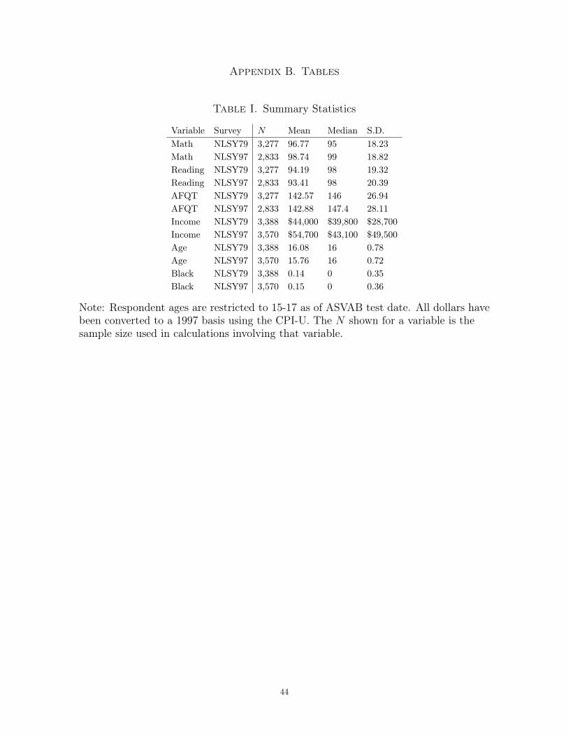
Appendix B. Tables

Table I. Summary Statistics

Variable Survey N Mean Median S.D.Math NLSY79 3,277 96.77 95 18.23Math NLSY97 2,833 98.74 99 18.82Reading NLSY79 3,277 94.19 98 19.32Reading NLSY97 2,833 93.41 98 20.39AFQT NLSY79 3,277 142.57 146 26.94AFQT NLSY97 2,833 142.88 147.4 28.11Income NLSY79 3,388 $44,000 $39,800 $28,700Income NLSY97 3,570 $54,700 $43,100 $49,500Age NLSY79 3,388 16.08 16 0.78Age NLSY97 3,570 15.76 16 0.72Black NLSY79 3,388 0.14 0 0.35Black NLSY97 3,570 0.15 0 0.36

Note: Respondent ages are restricted to 15-17 as of ASVAB test date. All dollars havebeen converted to a 1997 basis using the CPI-U. The N shown for a variable is thesample size used in calculations involving that variable.

44

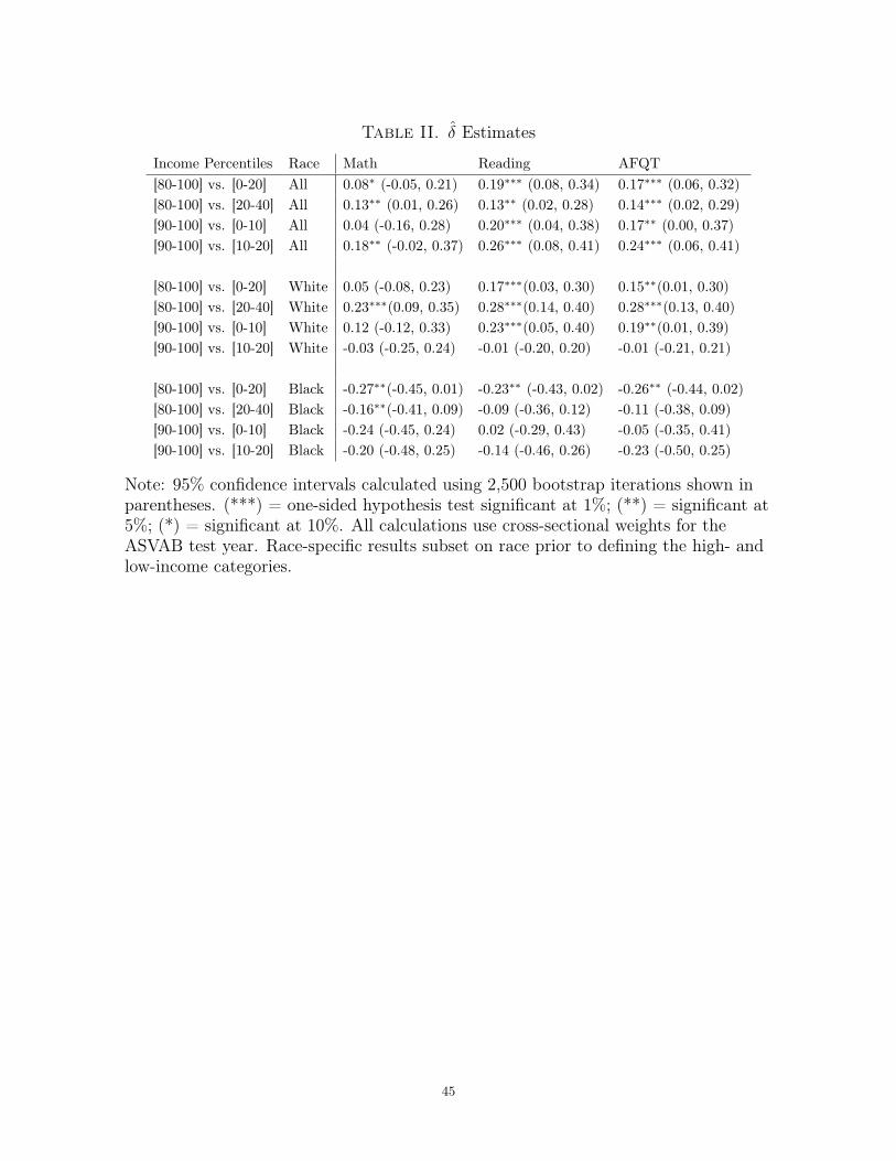
Table II. δ Estimates

Income Percentiles Race Math Reading AFQT[80-100] vs. [0-20] All 0.08∗ (-0.05, 0.21) 0.19∗∗∗ (0.08, 0.34) 0.17∗∗∗ (0.06, 0.32)[80-100] vs. [20-40] All 0.13∗∗ (0.01, 0.26) 0.13∗∗ (0.02, 0.28) 0.14∗∗∗ (0.02, 0.29)[90-100] vs. [0-10] All 0.04 (-0.16, 0.28) 0.20∗∗∗ (0.04, 0.38) 0.17∗∗ (0.00, 0.37)[90-100] vs. [10-20] All 0.18∗∗ (-0.02, 0.37) 0.26∗∗∗ (0.08, 0.41) 0.24∗∗∗ (0.06, 0.41)

[80-100] vs. [0-20] White 0.05 (-0.08, 0.23) 0.17∗∗∗(0.03, 0.30) 0.15∗∗(0.01, 0.30)[80-100] vs. [20-40] White 0.23∗∗∗(0.09, 0.35) 0.28∗∗∗(0.14, 0.40) 0.28∗∗∗(0.13, 0.40)[90-100] vs. [0-10] White 0.12 (-0.12, 0.33) 0.23∗∗∗(0.05, 0.40) 0.19∗∗(0.01, 0.39)[90-100] vs. [10-20] White -0.03 (-0.25, 0.24) -0.01 (-0.20, 0.20) -0.01 (-0.21, 0.21)

[80-100] vs. [0-20] Black -0.27∗∗(-0.45, 0.01) -0.23∗∗ (-0.43, 0.02) -0.26∗∗ (-0.44, 0.02)[80-100] vs. [20-40] Black -0.16∗∗(-0.41, 0.09) -0.09 (-0.36, 0.12) -0.11 (-0.38, 0.09)[90-100] vs. [0-10] Black -0.24 (-0.45, 0.24) 0.02 (-0.29, 0.43) -0.05 (-0.35, 0.41)[90-100] vs. [10-20] Black -0.20 (-0.48, 0.25) -0.14 (-0.46, 0.26) -0.23 (-0.50, 0.25)

Note: 95% confidence intervals calculated using 2,500 bootstrap iterations shown inparentheses. (***) = one-sided hypothesis test significant at 1%; (**) = significant at5%; (*) = significant at 10%. All calculations use cross-sectional weights for theASVAB test year. Race-specific results subset on race prior to defining the high- andlow-income categories.

45

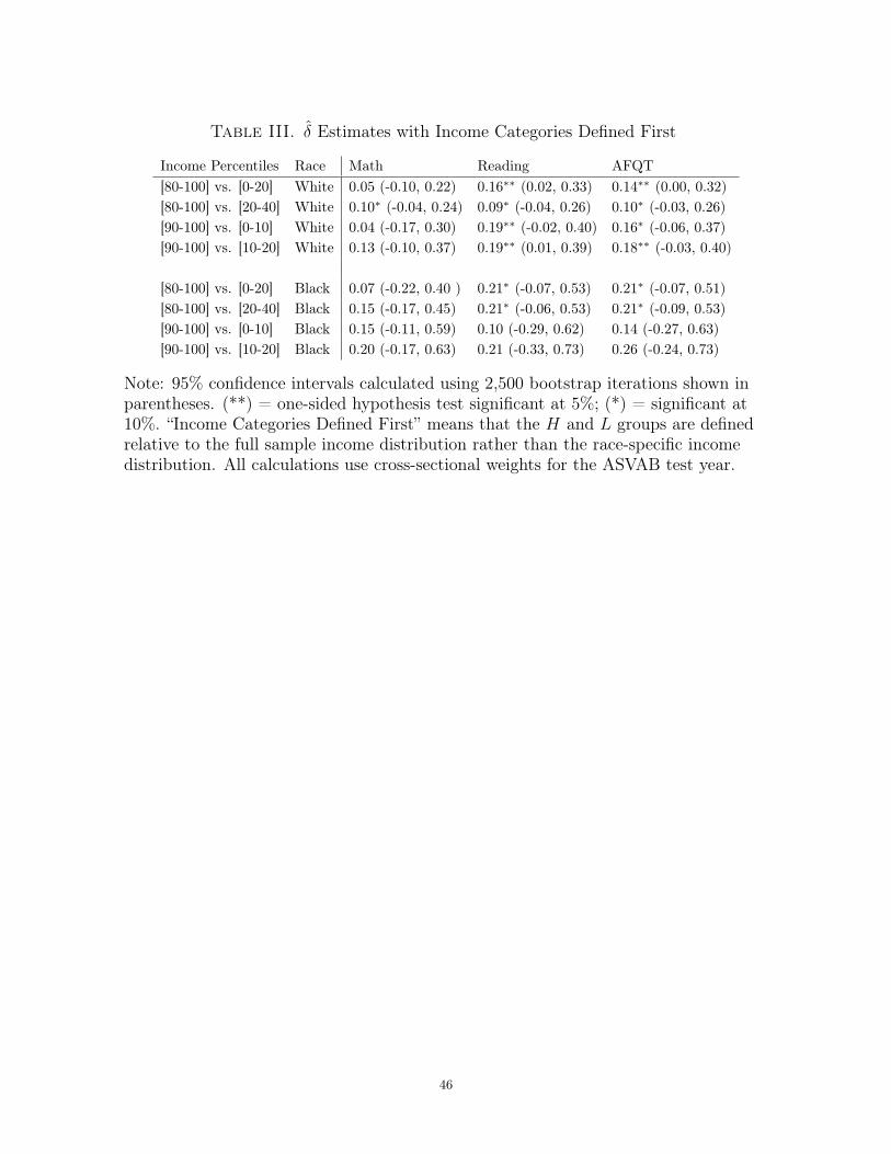
Table III. δ Estimates with Income Categories Defined First

Income Percentiles Race Math Reading AFQT[80-100] vs. [0-20] White 0.05 (-0.10, 0.22) 0.16∗∗ (0.02, 0.33) 0.14∗∗ (0.00, 0.32)[80-100] vs. [20-40] White 0.10∗ (-0.04, 0.24) 0.09∗ (-0.04, 0.26) 0.10∗ (-0.03, 0.26)[90-100] vs. [0-10] White 0.04 (-0.17, 0.30) 0.19∗∗ (-0.02, 0.40) 0.16∗ (-0.06, 0.37)[90-100] vs. [10-20] White 0.13 (-0.10, 0.37) 0.19∗∗ (0.01, 0.39) 0.18∗∗ (-0.03, 0.40)

[80-100] vs. [0-20] Black 0.07 (-0.22, 0.40 ) 0.21∗ (-0.07, 0.53) 0.21∗ (-0.07, 0.51)[80-100] vs. [20-40] Black 0.15 (-0.17, 0.45) 0.21∗ (-0.06, 0.53) 0.21∗ (-0.09, 0.53)[90-100] vs. [0-10] Black 0.15 (-0.11, 0.59) 0.10 (-0.29, 0.62) 0.14 (-0.27, 0.63)[90-100] vs. [10-20] Black 0.20 (-0.17, 0.63) 0.21 (-0.33, 0.73) 0.26 (-0.24, 0.73)

Note: 95% confidence intervals calculated using 2,500 bootstrap iterations shown inparentheses. (**) = one-sided hypothesis test significant at 5%; (*) = significant at10%. “Income Categories Defined First” means that the H and L groups are definedrelative to the full sample income distribution rather than the race-specific incomedistribution. All calculations use cross-sectional weights for the ASVAB test year.

46

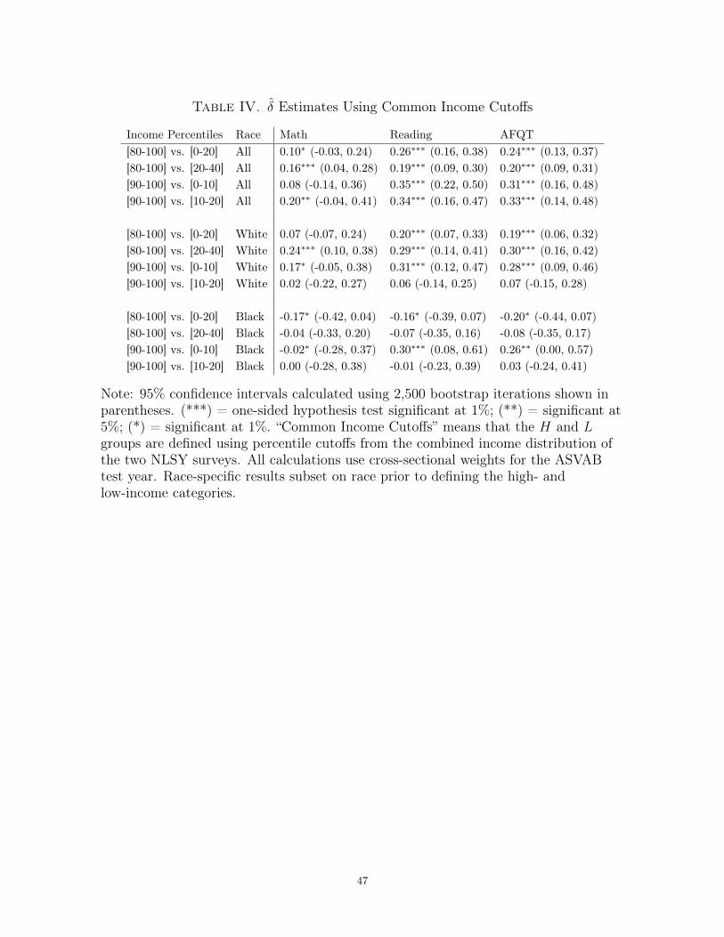
Table IV. δ Estimates Using Common Income Cutoffs

Income Percentiles Race Math Reading AFQT[80-100] vs. [0-20] All 0.10∗ (-0.03, 0.24) 0.26∗∗∗ (0.16, 0.38) 0.24∗∗∗ (0.13, 0.37)[80-100] vs. [20-40] All 0.16∗∗∗ (0.04, 0.28) 0.19∗∗∗ (0.09, 0.30) 0.20∗∗∗ (0.09, 0.31)[90-100] vs. [0-10] All 0.08 (-0.14, 0.36) 0.35∗∗∗ (0.22, 0.50) 0.31∗∗∗ (0.16, 0.48)[90-100] vs. [10-20] All 0.20∗∗ (-0.04, 0.41) 0.34∗∗∗ (0.16, 0.47) 0.33∗∗∗ (0.14, 0.48)

[80-100] vs. [0-20] White 0.07 (-0.07, 0.24) 0.20∗∗∗ (0.07, 0.33) 0.19∗∗∗ (0.06, 0.32)[80-100] vs. [20-40] White 0.24∗∗∗ (0.10, 0.38) 0.29∗∗∗ (0.14, 0.41) 0.30∗∗∗ (0.16, 0.42)[90-100] vs. [0-10] White 0.17∗ (-0.05, 0.38) 0.31∗∗∗ (0.12, 0.47) 0.28∗∗∗ (0.09, 0.46)[90-100] vs. [10-20] White 0.02 (-0.22, 0.27) 0.06 (-0.14, 0.25) 0.07 (-0.15, 0.28)

[80-100] vs. [0-20] Black -0.17∗ (-0.42, 0.04) -0.16∗ (-0.39, 0.07) -0.20∗ (-0.44, 0.07)[80-100] vs. [20-40] Black -0.04 (-0.33, 0.20) -0.07 (-0.35, 0.16) -0.08 (-0.35, 0.17)[90-100] vs. [0-10] Black -0.02∗ (-0.28, 0.37) 0.30∗∗∗ (0.08, 0.61) 0.26∗∗ (0.00, 0.57)[90-100] vs. [10-20] Black 0.00 (-0.28, 0.38) -0.01 (-0.23, 0.39) 0.03 (-0.24, 0.41)

Note: 95% confidence intervals calculated using 2,500 bootstrap iterations shown inparentheses. (***) = one-sided hypothesis test significant at 1%; (**) = significant at5%; (*) = significant at 1%. “Common Income Cutoffs” means that the H and Lgroups are defined using percentile cutoffs from the combined income distribution ofthe two NLSY surveys. All calculations use cross-sectional weights for the ASVABtest year. Race-specific results subset on race prior to defining the high- andlow-income categories.

47

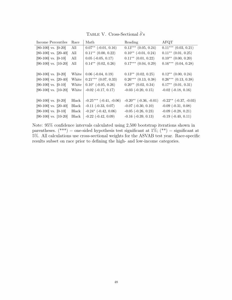
Table V. Cross-Sectional δ’s

Income Percentiles Race Math Reading AFQT[80-100] vs. [0-20] All 0.07∗∗ (-0.01, 0.16) 0.13∗∗∗ (0.05, 0.24) 0.11∗∗∗ (0.03, 0.21)[80-100] vs. [20-40] All 0.11∗∗ (0.00, 0.22) 0.10∗∗ (-0.01, 0.24) 0.11∗∗ (0.01, 0.25)[90-100] vs. [0-10] All 0.05 (-0.05, 0.17) 0.11∗∗ (0.01, 0.22) 0.10∗∗ (0.00, 0.20)[90-100] vs. [10-20] All 0.14∗∗ (0.02, 0.26) 0.17∗∗∗ (0.04, 0.29) 0.16∗∗∗ (0.04, 0.28)

[80-100] vs. [0-20] White 0.06 (-0.04, 0.19) 0.13∗∗ (0.02, 0.25) 0.12∗∗ (0.00, 0.24)[80-100] vs. [20-40] White 0.21∗∗∗ (0.07, 0.33) 0.26∗∗∗ (0.13, 0.38) 0.26∗∗∗ (0.13, 0.38)[90-100] vs. [0-10] White 0.10∗ (-0.05, 0.26) 0.20∗∗ (0.02, 0.34) 0.17∗∗ (0.01, 0.31)[90-100] vs. [10-20] White -0.02 (-0.17, 0.17) -0.03 (-0.20, 0.15) -0.02 (-0.18, 0.16)

[80-100] vs. [0-20] Black -0.25∗∗∗ (-0.41, -0.06) -0.20∗∗ (-0.36, -0.01) -0.22∗∗ (-0.37, -0.03)[80-100] vs. [20-40] Black -0.11 (-0.33, 0.07) -0.07 (-0.30, 0.10) -0.09 (-0.31, 0.08)[90-100] vs. [0-10] Black -0.24∗ (-0.42, 0.06) -0.05 (-0.26, 0.23) -0.09 (-0.28, 0.21)[90-100] vs. [10-20] Black -0.22 (-0.42, 0.09) -0.16 (-0.39, 0.13) -0.19 (-0.40, 0.11)

Note: 95% confidence intervals calculated using 2,500 bootstrap iterations shown inparentheses. (***) = one-sided hypothesis test significant at 1%; (**) = significant at5%. All calculations use cross-sectional weights for the ASVAB test year. Race-specificresults subset on race prior to defining the high- and low-income categories.

48

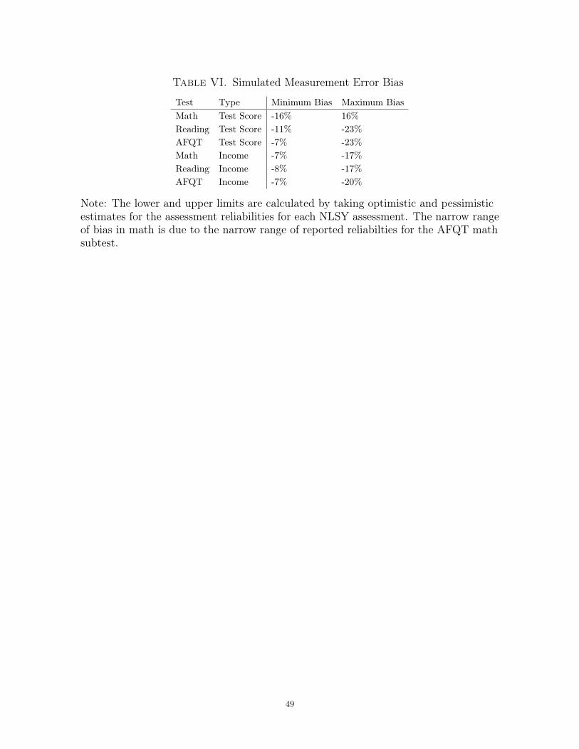
Table VI. Simulated Measurement Error Bias

Test Type Minimum Bias Maximum BiasMath Test Score -16% 16%Reading Test Score -11% -23%AFQT Test Score -7% -23%Math Income -7% -17%Reading Income -8% -17%AFQT Income -7% -20%

Note: The lower and upper limits are calculated by taking optimistic and pessimisticestimates for the assessment reliabilities for each NLSY assessment. The narrow rangeof bias in math is due to the narrow range of reported reliabilties for the AFQT mathsubtest.

49

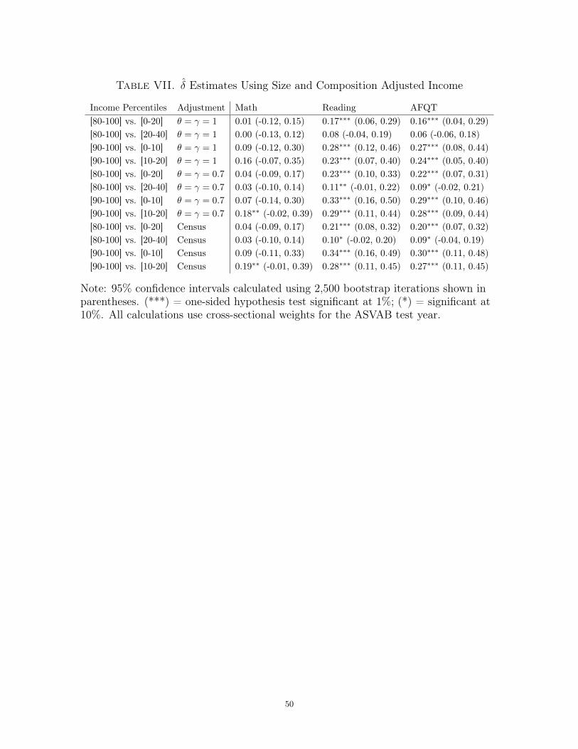
Table VII. δ Estimates Using Size and Composition Adjusted Income

Income Percentiles Adjustment Math Reading AFQT[80-100] vs. [0-20] θ = γ = 1 0.01 (-0.12, 0.15) 0.17∗∗∗ (0.06, 0.29) 0.16∗∗∗ (0.04, 0.29)[80-100] vs. [20-40] θ = γ = 1 0.00 (-0.13, 0.12) 0.08 (-0.04, 0.19) 0.06 (-0.06, 0.18)[90-100] vs. [0-10] θ = γ = 1 0.09 (-0.12, 0.30) 0.28∗∗∗ (0.12, 0.46) 0.27∗∗∗ (0.08, 0.44)[90-100] vs. [10-20] θ = γ = 1 0.16 (-0.07, 0.35) 0.23∗∗∗ (0.07, 0.40) 0.24∗∗∗ (0.05, 0.40)[80-100] vs. [0-20] θ = γ = 0.7 0.04 (-0.09, 0.17) 0.23∗∗∗ (0.10, 0.33) 0.22∗∗∗ (0.07, 0.31)[80-100] vs. [20-40] θ = γ = 0.7 0.03 (-0.10, 0.14) 0.11∗∗ (-0.01, 0.22) 0.09∗ (-0.02, 0.21)[90-100] vs. [0-10] θ = γ = 0.7 0.07 (-0.14, 0.30) 0.33∗∗∗ (0.16, 0.50) 0.29∗∗∗ (0.10, 0.46)[90-100] vs. [10-20] θ = γ = 0.7 0.18∗∗ (-0.02, 0.39) 0.29∗∗∗ (0.11, 0.44) 0.28∗∗∗ (0.09, 0.44)[80-100] vs. [0-20] Census 0.04 (-0.09, 0.17) 0.21∗∗∗ (0.08, 0.32) 0.20∗∗∗ (0.07, 0.32)[80-100] vs. [20-40] Census 0.03 (-0.10, 0.14) 0.10∗ (-0.02, 0.20) 0.09∗ (-0.04, 0.19)[90-100] vs. [0-10] Census 0.09 (-0.11, 0.33) 0.34∗∗∗ (0.16, 0.49) 0.30∗∗∗ (0.11, 0.48)[90-100] vs. [10-20] Census 0.19∗∗ (-0.01, 0.39) 0.28∗∗∗ (0.11, 0.45) 0.27∗∗∗ (0.11, 0.45)

Note: 95% confidence intervals calculated using 2,500 bootstrap iterations shown inparentheses. (***) = one-sided hypothesis test significant at 1%; (*) = significant at10%. All calculations use cross-sectional weights for the ASVAB test year.

50

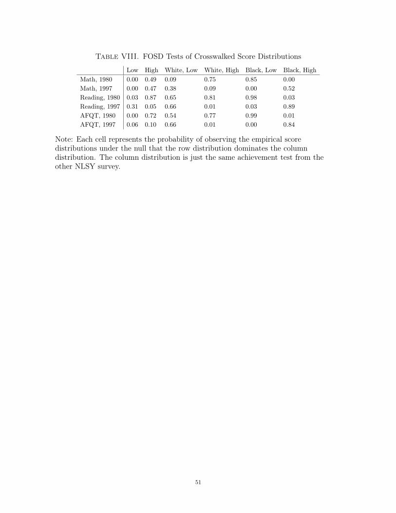
Table VIII. FOSD Tests of Crosswalked Score Distributions

Low High White, Low White, High Black, Low Black, HighMath, 1980 0.00 0.49 0.09 0.75 0.85 0.00Math, 1997 0.00 0.47 0.38 0.09 0.00 0.52Reading, 1980 0.03 0.87 0.65 0.81 0.98 0.03Reading, 1997 0.31 0.05 0.66 0.01 0.03 0.89AFQT, 1980 0.00 0.72 0.54 0.77 0.99 0.01AFQT, 1997 0.06 0.10 0.66 0.01 0.00 0.84

Note: Each cell represents the probability of observing the empirical scoredistributions under the null that the row distribution dominates the columndistribution. The column distribution is just the same achievement test from theother NLSY survey.

51

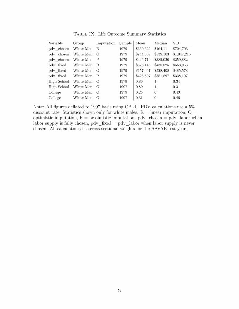
Table IX. Life Outcome Summary Statistics

Variable Group Imputation Sample Mean Median S.D.pdv_chosen White Men R 1979 $660,622 $464,11 $704,703pdv_chosen White Men O 1979 $744,669 $539,103 $1,047,215pdv_chosen White Men P 1979 $446,719 $385,020 $259,882pdv_fixed White Men R 1979 $578,148 $438,825 $563,953pdv_fixed White Men O 1979 $657,067 $528,408 $485,578pdv_fixed White Men P 1979 $425,897 $351,897 $338,197High School White Men O 1979 0.86 1 0.34High School White Men O 1997 0.89 1 0.31College White Men O 1979 0.25 0 0.43College White Men O 1997 0.31 0 0.46

Note: All figures deflated to 1997 basis using CPI-U. PDV calculations use a 5%discount rate. Statistics shown only for white males. R = linear imputation, O =optimistic imputation, P = pessimistic imputation. pdv_chosen = pdv_labor whenlabor supply is fully chosen, pdv_fixed = pdv_labor when labor supply is neverchosen. All calculations use cross-sectional weights for the ASVAB test year.

52

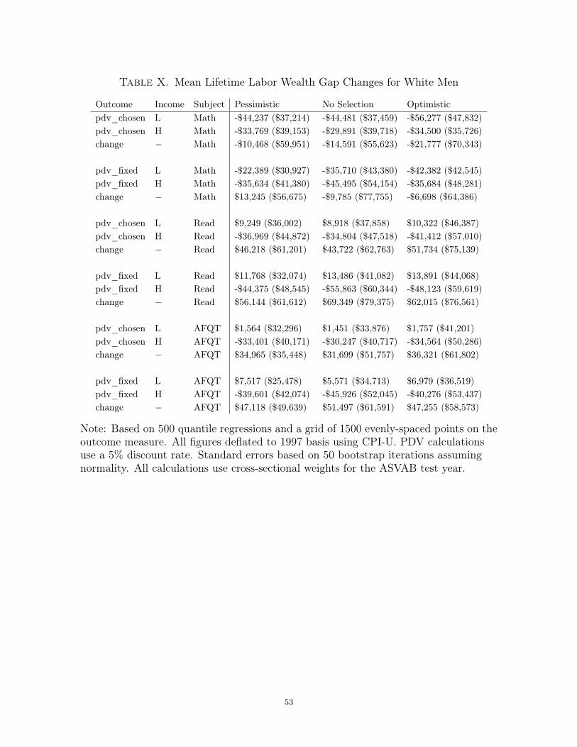
Table X. Mean Lifetime Labor Wealth Gap Changes for White Men

Outcome Income Subject Pessimistic No Selection Optimisticpdv_chosen L Math -$44,237 ($37,214) -$44,481 ($37,459) -$56,277 ($47,832)pdv_chosen H Math -$33,769 ($39,153) -$29,891 ($39,718) -$34,500 ($35,726)change − Math -$10,468 ($59,951) -$14,591 ($55,623) -$21,777 ($70,343)

pdv_fixed L Math -$22,389 ($30,927) -$35,710 ($43,380) -$42,382 ($42,545)pdv_fixed H Math -$35,634 ($41,380) -$45,495 ($54,154) -$35,684 ($48,281)change − Math $13,245 ($56,675) -$9,785 ($77,755) -$6,698 ($64,386)

pdv_chosen L Read $9,249 ($36,002) $8,918 ($37,858) $10,322 ($46,387)pdv_chosen H Read -$36,969 ($44,872) -$34,804 ($47,518) -$41,412 ($57,010)change − Read $46,218 ($61,201) $43,722 ($62,763) $51,734 ($75,139)

pdv_fixed L Read $11,768 ($32,074) $13,486 ($41,082) $13,891 ($44,068)pdv_fixed H Read -$44,375 ($48,545) -$55,863 ($60,344) -$48,123 ($59,619)change − Read $56,144 ($61,612) $69,349 ($79,375) $62,015 ($76,561)

pdv_chosen L AFQT $1,564 ($32,296) $1,451 ($33,876) $1,757 ($41,201)pdv_chosen H AFQT -$33,401 ($40,171) -$30,247 ($40,717) -$34,564 ($50,286)change − AFQT $34,965 ($35,448) $31,699 ($51,757) $36,321 ($61,802)

pdv_fixed L AFQT $7,517 ($25,478) $5,571 ($34,713) $6,979 ($36,519)pdv_fixed H AFQT -$39,601 ($42,074) -$45,926 ($52,045) -$40,276 ($53,437)change − AFQT $47,118 ($49,639) $51,497 ($61,591) $47,255 ($58,573)

Note: Based on 500 quantile regressions and a grid of 1500 evenly-spaced points on theoutcome measure. All figures deflated to 1997 basis using CPI-U. PDV calculationsuse a 5% discount rate. Standard errors based on 50 bootstrap iterations assumingnormality. All calculations use cross-sectional weights for the ASVAB test year.

53

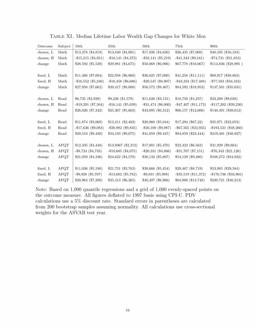
Table XI. Median Lifetime Labor Wealth Gap Changes for White Men

Outcome Subject 10th 25th 50th 75th 90th

chosen, L Math $13,378 ($4,819) $13,840 ($4,001) $17,926 ($4,630) $26,435 ($7,008) $40,105 ($16,183)chosen, H Math -$15,215 ($4,951) -$16,141 ($4,373) -$32,141 ($5,219) -$41,343 ($9,161) -$74,731 ($21,853)change Math $28,592 ($5,529) $29,981 ($4,675) $50,068 ($6,906) $67,778 ($10,067) $114,836 ($28,995 )

fixed, L Math $11,406 ($7,084) $22,958 ($6,960) $36,025 ($7,090) $41,258 ($11,111) $69,917 ($38,863)fixed, H Math -$16,552 ($5,240) -$16,458 ($6,686) -$20,547 ($8,907) -$43,334 ($17,488) -$77,583 ($34,163)change Math $27,958 ($7,662) $39,417 ($8,008) $56,572 ($9,467) $84,592 ($18,953) $147,501 ($35,031)

chosen, L Read $6,735 ($2,929) $9,226 ($1,579) $11,620 ($3,131) $18,750 ($4,237) $23,289 ($9,038)chosen, H Read -$19,291 ($7,504) -$16,141 ($5,039) -$31,474 ($6,000) -$47,407 ($11,173) -$117,202 ($39,230)change Read $26,026 ($7,342) $25,367 ($5,663) $43,095 ($6,312) $66,157 ($12,606) $140,491 ($39,612)

fixed, L Read $11,874 ($3,069) $13,211 ($2,402) $20,960 ($5,044) $17,294 ($67,22) $25,971 ($22,053)fixed, H Read -$17,636 ($9,083) -$20,982 ($9,835) -$20,100 ($9,987) -$67,565 ($22,935) -$193,521 ($48,260)change Read $29,510 ($9,430) $34,193 ($9,075) $41,059 ($9,447) $84,859 ($23,444) $219,491 ($48,927)

chosen, L AFQT $12,335 ($4,448) $13,9367 ($2,312) $17,801 ($5,470) $22,422 ($6,563) $31,929 ($9,864)chosen, H AFQT -$8,724 ($4,733) -$10,685 ($4,075) -$20,331 ($4,866) -$31,707 ($7,151) -$76,343 ($21,126)change AFQT $21,059 ($4,336) $24,622 ($4,579) $38,132 ($5,807) $54,129 ($9,480) $108,272 ($24,932)

fixed, L AFQT $11,036 ($5,190) $21,731 ($3,763) $30,666 ($5,454) $29,467 ($8,719) $53,985 ($29,584)fixed, H AFQT -$9,928 ($5,707) -$13,682 ($5,782) -$9,831 ($5,988) -$35,519 ($11,372) -$176,736 ($33,965)change AFQT $20,964 ($7,290) $35,413 ($6,365) $40,497 ($6,966) $64,986 ($13,748) $230,721 ($40,213)

Note: Based on 1,000 quantile regressions and a grid of 1,000 evenly-spaced points onthe outcome measure. All figures deflated to 1997 basis using CPI-U. PDVcalculations use a 5% discount rate. Standard errors in parentheses are calculatedfrom 200 bootstrap samples assuming normality. All calculations use cross-sectionalweights for the ASVAB test year.

54

Table XII. Probit-Estimated Mean School Completion Gap-Change Estimates

Outcome Group Skill Prices Math Reading AFQTHigh School White Men NLSY79 0.05 (0.03) 0.06 (0.03) 0.06 (0.04)High School White Men NLSY97 0.02 (0.02) 0.05 (0.03) 0.04 (0.03)College White Men NLSY79 0.07 (0.03) 0.07 (0.03) 0.07 (0.03)College White Men NLSY97 0.06 (0.02) 0.07 (0.03) 0.07 (0.03)

High School White Women NLSY79 -0.02 (0.03) -0.01 (0.03) -0.01 (0.03)High School White Women NLSY97 -0.02 (0.02) -0.01 (0.02) -0.01 (0.02)College White Women NLSY79 0.02 (0.02) -0.01 (0.03) 0.02 (0.03)College White Women NLSY97 0.02 (0.03) -0.02 (0.03) 0.01 (0.03)

High School Black Men NLSY79 -0.08 (0.08) 0.00 (0.08) -0.02 (0.08)High School Black Men NLSY97 -0.05 (0.08) 0.01 (0.08) -0.00 (0.09)College Black Men NLSY79 -0.03 (0.07) 0.04 (0.07) 0.01 (0.07)College Black Men NLSY97 -0.01 (0.07) 0.00 (0.04) -0.01 (0.04)

High School Black Women NLSY79 -0.04 (0.06) -0.04 (0.06) 0.00 (0.06)High School Black Women NLSY97 -0.03 (0.06) -0.04 (0.07) 0.00 (0.07)College Black Women NLSY79 -0.10 (0.07) -0.06 (0.05) -0.07 (0.06)College Black Women NLSY97 -0.09 (0.08) -0.06 (0.07) -0.07 (0.08)

Note: Based on 500 probit regressions and a grid of 3000 evenly-spaced points on theoutcome measure. Results use only optimistically-imputed data. Confidence intervalsbased on 200 bootstrap iterations assuming normality. All calculations usecross-sectional weights for the ASVAB test year.

55

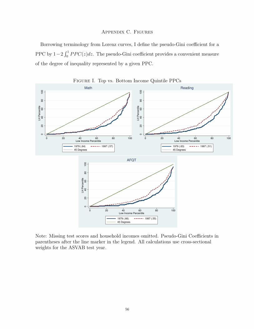
Appendix C. Figures

Borrowing terminology from Lorenz curves, I define the pseudo-Gini coefficient for a

PPC by 1−2´ 1

0PPC(z)dz. The pseudo-Gini coefficient provides a convenient measure

of the degree of inequality represented by a given PPC.

Figure I. Top vs. Bottom Income Quintile PPCs

020

40

60

80

100

LH

Perc

entile

0 20 40 60 80 100Low Income Percentile

1979 (.64) 1997 (.57)

45 Degrees

Math

020

40

60

80

100

LH

Perc

entile

0 20 40 60 80 100Low Income Percentile

1979 (.63) 1997 (.51)

45 Degrees

Reading0

20

40

60

80

100

LH

Perc

entile

0 20 40 60 80 100Low Income Percentile

1979 (.66) 1997 (.55)

45 Degrees

AFQT

Note: Missing test scores and household incomes omitted. Pseudo-Gini Coefficients inparentheses after the line marker in the legend. All calculations use cross-sectionalweights for the ASVAB test year.

56

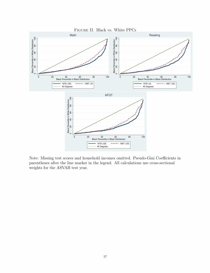
Figure II. Black vs. White PPCs0

20

40

60

80

100

Bla

ck P

erc

entile

in W

hite D

istr

ibution

0 20 40 60 80 100Black Percentile in Black Distribution

1979 (.56) 1997 (.5)

45 Degrees

Math

020

40

60

80

100

Bla

ck P

erc

entile

in W

hite D

istr

ibution

0 20 40 60 80 100Black Percentile in Black Distribution

1979 (.6) 1997 (.52)

45 Degrees

Reading

020

40

60

80

100

Bla

ck P

erc

entile

in W

hite D

istr

ibution

0 20 40 60 80 100Black Percentile in Black Distribution

1979 (.62) 1997 (.53)

45 Degrees

AFQT

Note: Missing test scores and household incomes omitted. Pseudo-Gini Coefficients inparentheses after the line marker in the legend. All calculations use cross-sectionalweights for the ASVAB test year.

57

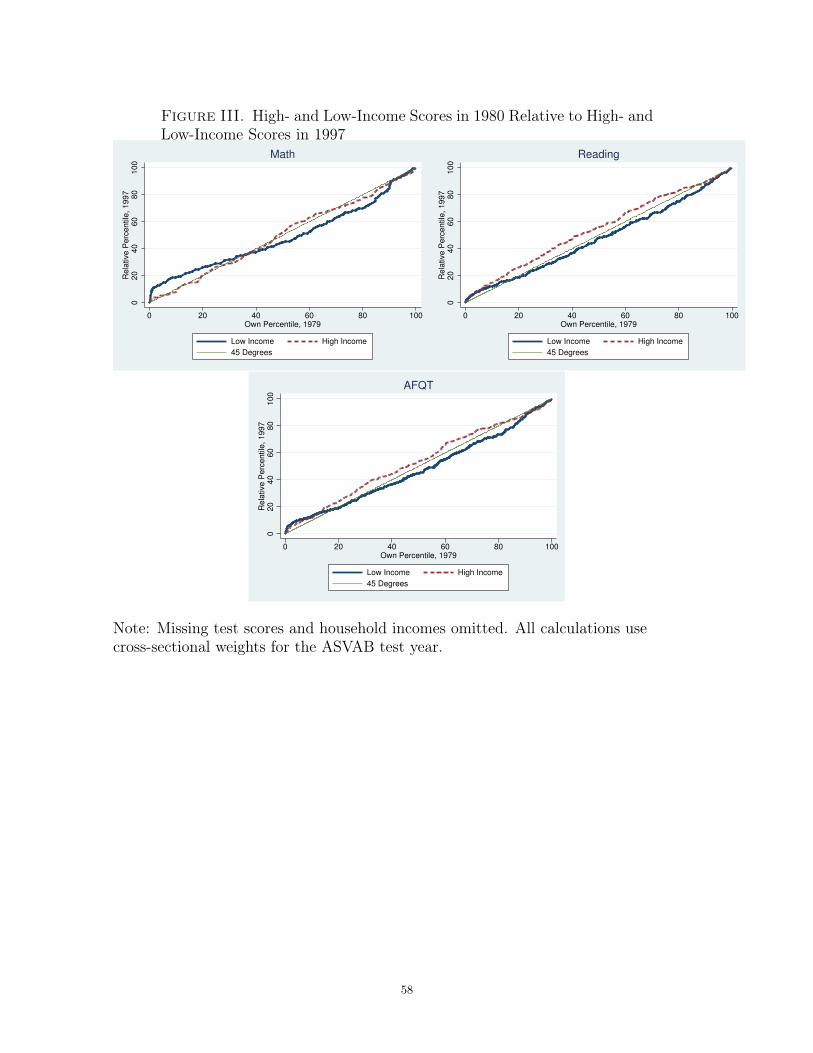
Figure III. High- and Low-Income Scores in 1980 Relative to High- andLow-Income Scores in 1997

020

40

60

80

100

Rela

tive P

erc

entile

, 1997

0 20 40 60 80 100Own Percentile, 1979

Low Income High Income

45 Degrees

Math

020

40

60

80

100

Rela

tive P

erc

entile

, 1997

0 20 40 60 80 100Own Percentile, 1979

Low Income High Income

45 Degrees

Reading

020

40

60

80

100

Rela

tive P

erc

entile

, 1997

0 20 40 60 80 100Own Percentile, 1979

Low Income High Income

45 Degrees

AFQT

Note: Missing test scores and household incomes omitted. All calculations usecross-sectional weights for the ASVAB test year.

58

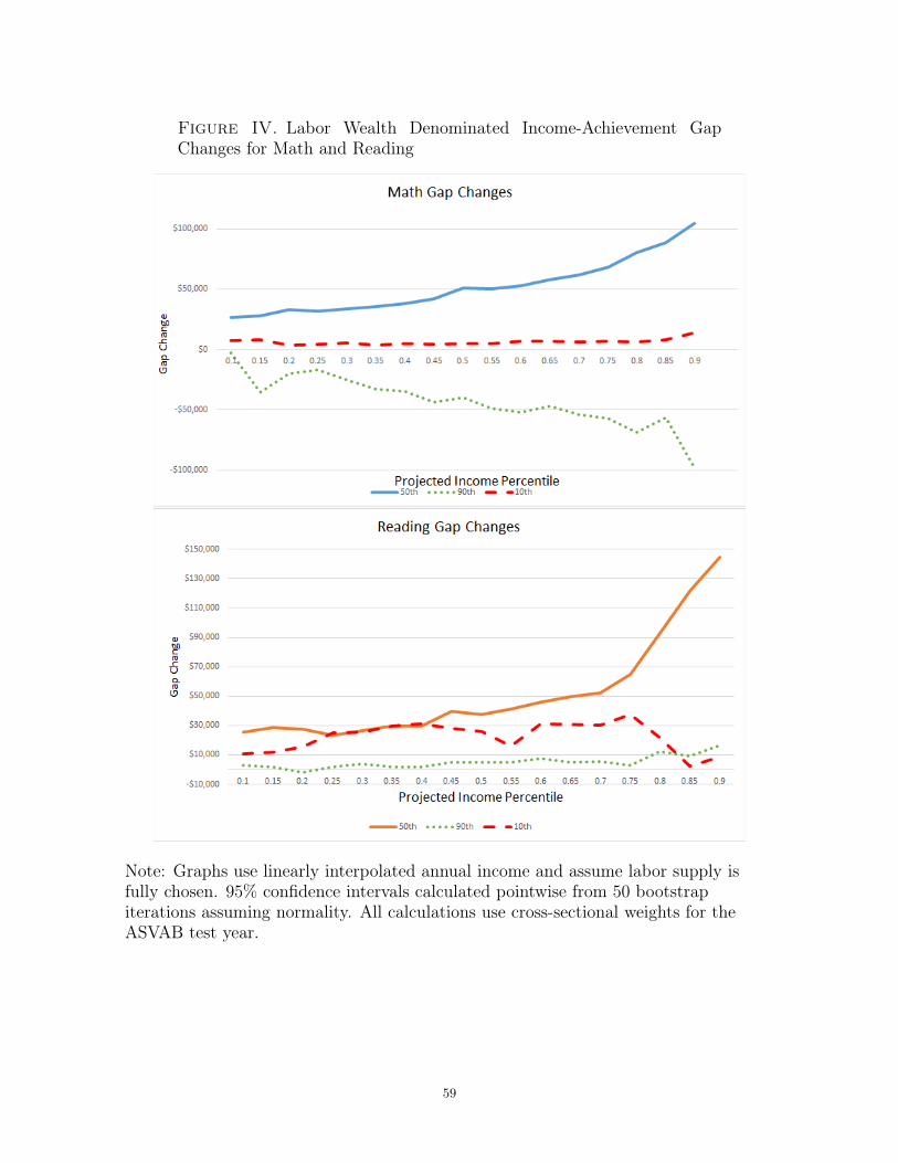
Figure IV. Labor Wealth Denominated Income-Achievement GapChanges for Math and Reading

Note: Graphs use linearly interpolated annual income and assume labor supply isfully chosen. 95% confidence intervals calculated pointwise from 50 bootstrapiterations assuming normality. All calculations use cross-sectional weights for theASVAB test year.

59

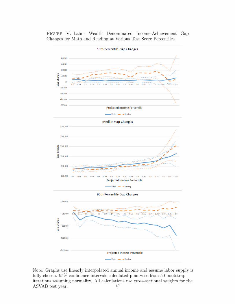
Figure V. Labor Wealth Denominated Income-Achievement GapChanges for Math and Reading at Various Test Score Percentiles

Note: Graphs use linearly interpolated annual income and assume labor supply isfully chosen. 95% confidence intervals calculated pointwise from 50 bootstrapiterations assuming normality. All calculations use cross-sectional weights for theASVAB test year. 60