Embed Size (px)
Citation preview

The influence of blended learningon students’ learning behavior with
respect to the heterogeneity ofstudents
Dissertation
zur Erlangung des akademischen Grades eines
Doktors der Wirtschaftswissenschaft
(Dr. rer. pol.)
durch die Fakultat fur Wirtschaftswissenschaften
der Universitat Duisburg-Essen
Campus Essen
vorgelegt von
Name: Yvonne Maria Braukhoff
Geburtsort: Tarnowitz (Polen)
Essen 2017

Tag der mundlichen Prufung: 04.04.2017
Erstgutachter: Prof. Dr. Erwin Amann
Zweitgutachter: Prof. Dr. Thomas Retzmann

Preface
I have written this dissertation during my employment as a research assistant at the
Chair of Microeconomics (Prof. Dr. Erwin Amann) at the University of Duisburg-
Essen. Throughout these challenging years, I have developed my academic skills and
met many people who I greatly esteem and to whom I am very grateful.
Special thanks go to my supervisor, Prof. Dr. Erwin Amann, who supported and
guided me during these years. At any time he devoted time to fruitful discussions
and suggestions and was open to new ideas. His support has always been helpful and
enriching. In addition, I am very thankful to Prof. Dr. Thomas Retzmann who did
not hesitate to be my second supervisor.
I am deeply grateful to my co-author, Marcel Braukhoff, who helped to create
a productive and illuminating working atmosphere and who always empowered me.
I also thank Ana Khazalashvili and Jan Schilling for proof-reading and being great
colleagues. I wish to thank Ilona Braun and Eva Zielke who were there for me at any
time and supported me with help and advice.
Most importantly, I am eternally grateful to my parents, family and friends who
always believed in me and supported me through all ups and downs. Their encourage-
ment made me strong and persistent.
I

Contents
Introduction 1
1 Impact of incentives and blended learning on students’ learning be-
havior 8
1.1 Introduction . . . . . . . . . . . . . . . . . . . . . . . . . . . . . . . . . 10
1.2 The model . . . . . . . . . . . . . . . . . . . . . . . . . . . . . . . . . . 12
1.2.1 The growth rate of skills . . . . . . . . . . . . . . . . . . . . . . 12
1.2.2 The exam and the utility function . . . . . . . . . . . . . . . . . 14
1.2.3 Utility maximization without mid-term examination . . . . . . . 15
1.2.4 Utility maximization with mid-term examination . . . . . . . . 26
1.2.5 Results . . . . . . . . . . . . . . . . . . . . . . . . . . . . . . . . 29
1.3 Conclusion . . . . . . . . . . . . . . . . . . . . . . . . . . . . . . . . . . 33
2 Influence of online feedback on students’ learning behavior 35
2.1 Introduction . . . . . . . . . . . . . . . . . . . . . . . . . . . . . . . . . 37
2.2 Feedback setting . . . . . . . . . . . . . . . . . . . . . . . . . . . . . . 39
2.3 The model . . . . . . . . . . . . . . . . . . . . . . . . . . . . . . . . . . 40
2.3.1 Optimal learning behavior . . . . . . . . . . . . . . . . . . . . . 40
2.3.2 Feedback on solving online exercises . . . . . . . . . . . . . . . . 43
2.3.3 Predicting optimal learning behavior . . . . . . . . . . . . . . . 45
2.3.4 Mid-term test . . . . . . . . . . . . . . . . . . . . . . . . . . . . 46
II

2.3.5 Updating learning behavior . . . . . . . . . . . . . . . . . . . . 47
2.3.6 Low-ability student . . . . . . . . . . . . . . . . . . . . . . . . . 53
2.3.7 Ungraded exams . . . . . . . . . . . . . . . . . . . . . . . . . . 58
2.3.8 Outlook . . . . . . . . . . . . . . . . . . . . . . . . . . . . . . . 61
2.4 Conclusion . . . . . . . . . . . . . . . . . . . . . . . . . . . . . . . . . . 63
3 Blended learning as response to student heterogeneity 65
3.1 Introduction . . . . . . . . . . . . . . . . . . . . . . . . . . . . . . . . . 67
3.2 Student heterogeneity . . . . . . . . . . . . . . . . . . . . . . . . . . . . 69
3.2.1 Dimensions of student heterogeneity . . . . . . . . . . . . . . . 69
3.2.2 Current measures to respond to student heterogeneity . . . . . . 71
3.3 The signaling mechanism in higher education . . . . . . . . . . . . . . . 71
3.3.1 Theoretical background . . . . . . . . . . . . . . . . . . . . . . . 72
3.3.2 Signals in higher education . . . . . . . . . . . . . . . . . . . . . 73
3.3.3 Self-assessment and dropout rate of students . . . . . . . . . . . 82
3.4 New measures as response . . . . . . . . . . . . . . . . . . . . . . . . . 84
3.4.1 Blended learning as response . . . . . . . . . . . . . . . . . . . . 84
3.4.2 JACK as example for blended learning . . . . . . . . . . . . . . 85
3.5 Conclusion . . . . . . . . . . . . . . . . . . . . . . . . . . . . . . . . . . 89
Conclusion 92
Bibliography 96
III

Introduction
The current learning environment is characterized by an increasing heterogeneity of
students and by a trend towards online learning.
In addition to a growing number of first year students, higher education has to
cope with various dimensions of student heterogeneity. Traditional sources of hetero-
geneity like skills, professional experience, social and cultural background are extended
by new dimensions (Hanft 2015). These new dimensions of heterogeneity are repre-
sented by a broader age span and by differences in organizing self-study among students
(Schulmeister et al. 2012). For this purpose, higher education has to rethink homo-
geneous university structures and traditional teaching methods, which do not fit the
current diversity. Until now, universities try to meet this increasing heterogeneity with
receiving inspections and preparatory courses, concentrating mainly on the start of
higher education studies (Hanft 2015). These measures try to transform heterogene-
ity into homogeneity instead of accepting the diversity of students. Hence, in order
to accept heterogeneous students, higher education might be forced to adapt course
structures (Biggs and Tang 2011; Wildt 2001). In this connection, the restructuring of
higher education within the Bologna process represents a possibility to pay attention
to heterogeneous students (EACEA 2012). The choice between bachelor’s and master’s
degrees considers different cognitive abilities and levels of commitment.
Besides the heterogeneity of students, today’s learning environment shows a new
trend towards online learning. Since traditional teaching methods are taken up by this
trend, blended learning is in the focus, being a mixture of face-to-face sessions and
1

INTRODUCTION 2
e-learning tools. Many studies show that e-learning tools have increased significantly
in the current learning experience of students (Allen and Seaman 2006). Furthermore,
students prefer to learn online and reduce their commitment in face-to-face education
(Garrison and Kanuka 2004; Sebastianelli and Tamimi 2011). Making use of online
learning tools, teachers who are confronted with a huge number of students benefit from
economies of scale and scope (Twigg 2013; Morris 2008). In addition, feedback which is
implemented in computer-supported learning has a positive influence on the students’
motivation and problem-solving (Zumbach and Reimann 2003). Assuming courses with
a considerable number of students, e-learning tools reduce the workload associated
with individual and immediate feedback. Furthermore, feedback plays a crucial role
in guiding the self-study and evaluating the learning progress. In this connection,
Dunning et al. (2004) show that most students have a flawed self-assessment and
especially overestimate their abilities. Furthermore, the decision to begin one’s studies
is driven by the self-perception of skills (Chevalier et al. 2009). Especially a high self-
perception promotes the investment in higher education and the danger of dropping
out. Thus, flawed self-perception justifies the need for feedback.
This dissertation examines the influence of blended learning on student’s learning
behavior with respect to student heterogeneity. The analysis is based on theoretical
models. Since blended learning offers a variety of learning opportunities which are
available around-the-clock, it is able to influence learning in a different way than tra-
ditional teaching methods. Especially online feedback helps students to self-regulate
learning and to assess their abilities. Taking the growing heterogeneity of students into
consideration, blended learning may be a measure to rethink homogeneous university
structures.
In the following, I will describe the assumed blended learning setting. Then, I will
give a brief overview of the theoretical concepts which are used in this dissertation. Af-
terwards, I will provide an outline of the studies which apply and extend the presented
theoretical background.

INTRODUCTION 3
Blended learning setting
The blended learning setting of all chapters is based on the courses of the Chair of
Microeconomics at the University of Duisburg-Essen. They use an online tool called
JACK, described in detail in Chapter 3. The e-learning tool is implemented in addi-
tion to traditional face-to-face sessions. While, weekly lectures and tutorial classes aim
to teach basic knowledge and demonstrate examples, the offer of e-learning exercises
represents a possibility of around-the-clock self-training and assessment of course con-
tents. The combination of traditional face-to-face sessions and e-learning opportunities
is called blended learning.
The described courses are characterized by a considerable number of students, plac-
ing new demands on teachers. In this context, e-learning opportunities are able to
reduce the workload of teachers. The e-learning tool offers online exercises which are
available around-the-clock and an online mid-term test with the possibility to improve
the final exam mark.
Online exercises guide students’ self-study, since they repeat every topic of the
course. Students are able to solve online exercises anywhere and around-the-clock and
receive an immediate feedback after handing in their solution. Variables are randomized
in order to offer a variety of possibilities to retain course contents. In addition to online
exercises, students have the possibility to take an online mid-term test and gain bonus
points for the final exam. Thereby, a failed mid-term test is not credited. In contrast
to this, a passed mid-term test only improves the final exam mark if the student passes
the final exam. The key advantage of e-learning tools is the fairness and the immediate
electronic correction. Since the correction of online exercises and mid-term tests is
carried out automatically, the workload remains small and objectivity is guaranteed.

INTRODUCTION 4
Theoretical background
This thesis is based on the concept of learning by doing (Arrow 1962; Gocke 2002) and
on Spence’s (1973) signaling model. Thereby, Chapter 1 and 2 apply learning by doing
to university courses and Chapter 3 uses Spence’s signaling model in order to analyze
the higher education system.
Arrow (1962) was the first author who introduced learning by doing to the eco-
nomic literature within the field of production. He describes learning as experience
which is gained during the process of problem-solving and activity. Thus, performance
improves over time based on intertemporal changes in production functions. As a re-
sult, knowledge is growing in time as a product of experience. Gocke (2002) takes up
the idea of learning by doing and introduces the optimal allocation of time between
working and leisure. He models learning as a by-product of working which is measured
by aggregated output in time. Thus, human capital accumulation depends on working
time which leads to learning and consumption of goods. Gocke assumes that utility
consists of leisure and of the consumption of goods. Nevertheless, working time is lim-
ited due to the optimal time allocation to working and leisure. Therefore, growth of
experience accumulation is limited because of consumption saturation effects in favor
of the expansion of leisure. In contrast to this, the production side shows constant
returns to scale on experience itself.
Chapter 1 and 2 apply this concept to university courses with the trade-off between
learning and leisure. In this context, utility is based on the final exam mark and the
disutility of learning. As a consequence, accumulation of skills is limited by passing
the exam with the best mark and by the desire to consume leisure.
The second theoretical strain is represented by Spence’s signaling model of 1973.
In this paper he firstly introduced the effects of signals on the job market which is
characterized by asymmetrical information. He assumes that the employer does not
know the productivity of the individual before hiring him. With the aim to counteract
this uncertainty, individuals can invest in education. Obtaining a degree serves as

INTRODUCTION 5
an observable signal for the employer, because it involves costs in terms of time and
money. Spence distinguishes two groups of highly and less productive individuals who
know their productivity. The employer believes that a critical level of education exists,
distinguishing between high- and low-ability individuals. Therefore, he pays a wage
which equals the individual productivity, since it is the contribution of the graduate
to the firm. According to this wage schedule, individuals choose their investments
in education with the aim to maximize their utility which is given by the difference
between wage and signaling-costs.
Chapter 3 applies this model to the current higher education system comprising
bachelor’s and master’s degrees. Since two possible investment in education exist, the
model is extended by a third productivity level.
Overview of chapters
Chapter 1 and Chapter 2 follow Gocke (2002) by applying his model of learning by
doing to the framework of university courses. These chapters analyze how learning
behavior is influenced by online learning opportunities. Chapter 3 introduces a broader
perspective, shedding light on the impact of blended learning on student heterogeneity
which characterizes today’s higher education system. In order to analyze the current
higher education system, Spence’s signaling model (1973) is extended by a third level
of productivity. While students’ learning behavior plays a central role in the first and
second Chapter, student heterogeneity is the main focus of Chapter 3.
Chapter 1 was created in collaboration with Erwin Amann and Marcel Braukhoff.
Chapter 2 is co-authored with Marcel Braukhoff and Chapter 3 is my own work.
The first chapter develops a simple model of learning by doing in the context of
university courses which is based on Gocke (2002). Thereby, exam marks are a result
of skills which are accumulated during the learning period. Students have the oppor-
tunity to repeat course contents whenever and how often they wish to, since blended

INTRODUCTION 6
learning creates around-the-clock learning opportunities. In this connection, e-learning
exercises help to improve the retention of newly acquired skills. In addition, mid-term
tests provide incentives for early learning, since they bear the possibility to improve
the final exam mark. While solving online exercises, students accumulate skills. This
accumulation of skills is limited by passing the exam with the best mark. Furthermore,
they face a trade-off between learning and leisure, since learning leads to a reduction
of leisure time. This trade-off curtails spending the total time for learning. Students
have perfect knowledge about their skill level and differ by preferences for learning.
While students with preferences for long-term learning prefer to learn constantly dur-
ing the learning period, students with preferences for short-term learning tend to do
last-minute learning. Utility is maximized for both types of students and the results for
the case with and without mid-term test are compared. In addition, continuity of learn-
ing activity during the learning period is analyzed. Finally, Chapter 1 addresses the
question how incentives and blended learning influence and improve learning behavior
of the student.
Chapter 2 extends this model by assuming that students have an imperfect knowl-
edge about their skill level. For this purpose, this chapter introduces the influence of
feedback. Online exercises and a mid-term test serve as sources of feedback since they
provide information about the individual skill level. Depending on the utilization of
feedback implemented in blended learning, students may check their learning progress
and individual skill level. As a first step, the influence of online exercises on the per-
ceived learning progress is analyzed. Secondly, we look at the impact of the mid-term
test as source of feedback on the perceived skill level. While students who do not
use blended learning base their learning time on their perceived skill level, students
using blended learning are able to compare their perceived skill level to the received
feedback. This evaluation of accumulated skills enables students to update their fur-
ther learning activity. For this purpose, dynamic utility maximization is analyzed in
the case of average and low-ability students. In addition, this analysis sheds light on

INTRODUCTION 7
the influence of feedback on utility. Consequently, this chapter addresses the question
how the feedback implemented in blended learning influences and improves learning
behavior and utility.
Chapter 3 introduces a new perspective by looking at blended learning and the
higher education system which is characterized by a growing heterogeneity of students.
For this purpose I give an overview over dimensions of student heterogeneity. There-
after, the higher education system which has been restructured within the framework
of the Bologna process is compared to previous systems with only one possible degree.
The choice between different degrees like the bachelor’s and master’s degree is a pos-
sibility to pay attention to student heterogeneity. In contrast to prior degrees, this
differentiated system gives students the possibility to choose different levels of higher
education degrees according to individual abilities and future plans. Since the com-
pleted degree serves as a signal for the employer and thereby reduces his uncertainty
concerning the productivity of the graduate, I apply Spence’s (1973) signaling model
in order to compare the signaling power of different degrees. Nevertheless, Spence’s
signaling model assumes perfect knowledge about individual skills, although dropout
rates in higher education indicate the opposite. Flawed self-assessment might be one
reason for this dropout rate. With the aim to implement new teaching routines in
higher education, Chapter 3 proposes blended learning as a response to the wrong
self-assessment and increasing heterogeneity of students. As support to traditional
face-to-face sessions, the online learning tool JACK is introduced and described in de-
tail. With reference to the described dimensions of student heterogeneity and with
the aim to correct flawed self-assessment, the gains of blended learning are depicted in
detail. Thus, this chapter analyzes dimensions of student heterogeneity and shows how
blended learning takes these dimensions into consideration and helps to correct flawed
self-assessment.

Chapter 1
Impact of incentives and blended
learning on students’ learning
behavior
Erwin Amann1
Marcel Braukhoff2
Yvonne Maria Braukhoff3
1Department of Economics, University of Duisburg-Essen, 45117 Essen Germany. Email:[email protected]
2Department of Mathematics, University of Cologne, 50931 Cologne Germany. Email:[email protected]
3Department of Economics, University of Duisburg-Essen, 45117 Essen Germany. Email:[email protected]
8

CHAPTER 1. INCENTIVES AND BLENDED LEARNING 9
Abstract
This paper focuses on a blended learning approach implemented in uni-
versity courses at the University of Duisburg-Essen with the aim to improve
the performance of students in the exam and the course of study. In addition
to the created online learning opportunities, an incentive-based approach
aims to promote student engagement in courses and gives the opportunity
to self-assess own skills. Due to this incentive-based blended learning con-
cept, the learning process has been proven to become more effective and
successful. Students tend to learn continuously and work off their back-
log. Additionally, students’ motivation to deal with the teaching material
rises. Consequently, the lack of preparation which often results in poor
performance decreases.
Exam outcomes are the result of training skills, which rise while solving
exercises and spending learning time. Additional learning opportunities,
automated feedback and hints help to reduce learning costs, to improve
the organization of individual learning time and to increase the students’
success. This paper uses a dynamic utility maximization approach consider-
ing the choice between learning time and leisure. Depending on individual
skills, on preferences for leisure time and for discounting, the individual
learning performance varies. Changing the opportunities and incentives
has a specific impact on overall learning time as well as on partitioning
learning time along the semester.
Hence, this paper introduces a specific model of accumulation of skills
and then emphasizes the importance of the interplay of incentives to learn,
e-learning opportunities and face-to-face sessions in regard to more efficient
learning behavior.

CHAPTER 1. INCENTIVES AND BLENDED LEARNING 10
1.1 Introduction
Since traditional teaching methods are taken up by the new trend towards online
learning, blended learning becomes more important. Blended learning combines face-
to-face sessions and e-learning opportunities and thus meets these growing expectations
and needs for better learning opportunities and outcomes (Garrison and Kanuka 2004).
This trend is confirmed by various surveys which show that online learning tools in
students’ learning experiences have increased significantly (Allen and Seaman 2006).
In Germany, for example, nearly every University offers e-learning platforms (Henning
2015).
The significant growth rate of online learning strategies is driven by supply and
demand side reasons. On the one hand, university teachers benefit from economies of
scale and scope in teaching a large number of students (Twigg 2013; Morris 2008). On
the other hand, students show a new attitude towards online learning (Sebastianelli
and Tamimi 2011) and a reduced engagement with face-to-face education (Exetere et
al. 2010).
Furthermore, students are characterized by an increasing heterogeneity these days
(Hanft 2015). Besides social differences, students show diverging cognitive abilities and
commitment levels. The homogeneous university structures and teaching methods are
confronted with these heterogeneous student characteristics. Nevertheless, most initi-
ated actions only affect the access to higher education studies like receiving inspections
and take no account of teaching routines. In the future higher education has to cope
with new demands concerning student heterogeneity.
In order to develop a simple model, this paper makes use of the concept of learning
by doing to show the influence of blended learning on learning behavior. Until now,
economic literature has only focused on learning by doing within the field of production.
In this context, learning by doing was first introduced in 1962 by Arrow, who describes
learning as a product of experiences which are gained during the process of problem-
solving and activity. Thus, production functions underlie intertemporal changes in

CHAPTER 1. INCENTIVES AND BLENDED LEARNING 11
skills. As a result, skills are growing in time due to improvement in performance.
Gocke (2002) extends this model by analyzing the optimal allocation of time be-
tween work and leisure in the context of learning by doing. Furthermore, he models an
experience curve which characterizes learning as a by-product of working. Thus, expe-
rience as human capital is accumulated via learning by doing and depends on working
time and the consumption of goods. The author concludes that the rise in productivity
is utilized for an expanding leisure time. Therefore, growth of experience accumulation
is limited by utility side reasons, whereas the production side shows constant returns
to scale on experience itself.
This paper introduces a simple model of learning by doing in the context of univer-
sity courses. The exam outcome depends on the skill accumulation during the learning
period. Thereby, blended learning creates additional learning opportunities which are
available 24 hours per day during 7 days per week. E-learning exercises take student
heterogeneity into account, since they are characterized by a high flexibility of time
and space and since they offer many possibilities to improve the retention of newly-
acquired skills. In addition, mid-term examinations provide incentives to continuous
learning and consequently boost the commitment in blended learning with the help of
rewards. While solving blended learning exercises, students acquire skills and human
capital is accumulated, hereafter called skills in this paper. However, students have to
decide upon the optimal time allocation to learning and leisure which differs in utility
formulation. This model shows similarities to Gocke (2002), yet learning by doing is
applied to university courses instead of production. Furthermore, the choice between
working/learning and leisure is not the only concern of this paper. This trade-off just
curtails the overall spending of time for learning.
Thus, we address the question how incentive and blended learning influence and
improve learning behavior.

CHAPTER 1. INCENTIVES AND BLENDED LEARNING 12
1.2 The model
This paper introduces the concept of learning by doing to university courses supported
by incentive-oriented blended learning. Besides face-to-face sessions students have
the possibility to solve online exercises during the semester in order to improve their
skills with the overall aim to pass the exam. These online exercises take student
heterogeneity into account, since they offer different levels of difficulty, individual hints
and are characterized by a high flexibility of time and space and last but not least offer
possibilities to repeat course contents.
1.2.1 The growth rate of skills
In this model the accumulation of skills via learning by doing is the result of solving
exercises. In this first approach we assume that a student uses the blended learning
platform to improve his skills. The relative learning time q = q(t) describes the fraction
of time a student spends using learning opportunities at time t during the semester.
Overall time is split into learning time q(t) ∈ [0, 1] and leisure 1− q(t). Let E(ξ, q) be
the number of exercises solved by a student per time unit.
The number of exercises students can solve per time unit depends on their expertise
and the time spent for learning. It is assumed that both increasing time and skills has
a positive impact on E:
∂E
∂ξ(ξ, q) ≥ 0,
∂E
∂q(ξ, q) > 0.
In the sequel, we work with a simplified model and suppose that E is bilinear in ξ
and q, i.e. we have
E(ξ, q) = eqξ with e = const.
The learning parameter e differs between students but also can be positively affected
by improving learning opportunities. Moreover, we assume that skills ξ are differen-

CHAPTER 1. INCENTIVES AND BLENDED LEARNING 13
tiable in time t and induced by the exercises solved fulfilling the ordinary differential
equationd
dtξ = A(E, q, ξ),
for some differentiable function A depending on the learning activity of the student
and his current skills. Assuming that A is linear in E and does not directly depend on
ξ, A(E, q, ξ) = a(q) · E(ξ, q), we can rewrite
d
dtξ = a(q) · eq · ξ (1.1)
and interpret a(q) · eq as the growth rate of the skills. Keeping this in mind, a models
the productivity. We suppose
∂a
∂q(q) R 0 whenever q R q0
for some q0 ∈ (0, 1). However, if a critical relative learning time q0 is exceeded, the
productivity decreases due to the absence of pauses. In the following, we apply a simple
approach for the learning productivity by choosing
a(q) = q(1− q).
Now, we can directly solve Equation (1.1) by
ξ(t) = ξ0 exp
(e
∫ t
0
q(s)2(1− q(s))ds).
As we see, skills start with an individual initial skill level ξ0 and are accumulated during
the semester as a result of solving online exercises E.

CHAPTER 1. INCENTIVES AND BLENDED LEARNING 14
1.2.2 The exam and the utility function
Utility is a result of accumulated skills and leisure as the residual of learning time. We
assume quasi linear utility of a student writing the exam at time T
u := Xe−δT − γ∫ T
0
q(t)e−δtdt
for some γ, δ ≥ 0 and 0 < t0 < T , where X is the result of the exam. We use the
convention that X = 1 represents the best mark and X = X0 = 12
the minimal mark
for a student to pass the exam. Therefore X ∈ {0} ∪ [12, 1], where X = 0 means failed.
Utility decreases with time spent on learning q, since a high learning activity results
in less leisure time. Furthermore, the term e−δt models individual time preferences,
where δ ≥ 0 specifies the individual discount rate. δ = 0 implies no discounting of the
future. Large values of delta implies a decrease of the valuation of the exam at the
beginning of the semester. Students with high δ rather prefer intensive learning at the
end of the semester instead of regular learning during the semester.
The result of the exam depends on the skills of the student at time T and thus, we
interpret X as a function of ξ. However, this dependency is not perfectly given, since it
is not possible for the student to exactly predict the result of the exam before actually
writing it. Therefore, we introduce an additional parameter ε for the uncertainty
modeling good luck or bad luck, concentration and further unpredictable influences.
Definition 1. The function
X(ξ, ε) =
0 if ξ + ε < 1
2,
1 if ξ + ε > 1,
ξ + ε else
(1.2)
describes the result function of the exam.

CHAPTER 1. INCENTIVES AND BLENDED LEARNING 15
We can thus rewrite the utility function as
u(q, ε) = X(ξ(T ), ε)e−δT − γ∫ T
0
q(t)e−δtdt.
1.2.3 Utility maximization without mid-term examination
Since the only choice in this model is on the time spent on learning and leisure, utility
is maximized by dynamic optimization in q(t). As a baseline, we first determine the
optimal choice of learning time q without taking a mid-term examination into account.
Section 1.2.4 then examines dynamic optimization with mid-term examination in order
to identify the specific incentives.
The resulting function of the exam X(ξ, ε) includes four cases, leading to different
utility-maximizing time allocations q. We start with a student reaching in equilibrium
a positive but not the best result with certainty. The second case describes students
who fail the exam with certainty. The third case deals with students having a positive
probability to fail and last, students who pass the exam with positive probability
reaching the best score. We have chosen this order with the aim to start with the
average and most common student.
Optimal time allocation for an average student
The first case deals with an average student. This case is given by 12< ξ(T ) + ε < 1.
Given that X(ξ, ε) = ξ + ε, we can derive the utility function as
u(q, ε) = (ξ(T ) + ε)e−δT − γ∫ T
0
q(t)e−δtdt. (1.3)
The disutility of learning at time t given by γq(t)e−δt decreases for increasing δ and t.

CHAPTER 1. INCENTIVES AND BLENDED LEARNING 16
In order to maximize the utility in (1.3), we derive the first order condition
d
dsu(q + sv)
∣∣s=0
= e−δT ξ0e
∫ T
0
(2qv − 3q2v)dt · exp
(e
∫ T
0
q2(1− q)dt)− γ
∫ T
0
veδtdt
=
∫ T
0
v
(ξ0eq(2− 3q) exp
(e
∫ T
0
q2(1− q)dt′ − δT)− γe−δt
)dt
!= 0
for all v = v(t). Inserting the delta-function v(t) = δτ (t) defined by
∫ T
0
δτf(t)dt = f(τ),
it follows that
ξ0eq(t)(2− 3q(t)) exp
(e
∫ T
0
q2(1− q)dt′ − δT)
= γe−δt.
Note that the factor exp e∫ T
0q2(1− q)dt′ is independent from time t. Defining
C := 3γ
ξ0eexp
(−e∫ T
0
q2(1− q)dt+ δT
)(1.4)
entails
q(t)2 − 2
3q(t) +
1
9Ce−δt = 0.
This equation only has a real-valued solution if Ce−δt ≤ 1. For C ≤ 1, the optimal q
is given by
q(t) =1
3
(1 +
√1− Ce−δt
), (1.5)

CHAPTER 1. INCENTIVES AND BLENDED LEARNING 17
since the second order condition for a maximum,
0 ≥ d2
ds2u(q + sv)
∣∣s=0
= ξ0
∫ T
0
2v2(1− 3q)dt exp
(∫ T
0
q2(1− q)dt− δT)
+ ξ0
(∫ T
0
v(2q − 3q2)dt
)2
exp
(∫ T
0
q2(1− q)dt− δT),
ensures q ≥ 13: The second term is always non-negative such that the first term has to
be ≤ 0 for a utility maximum leading to q ≥ 13. The constant C can be computed by
solving Equation (1.4) after inserting Equation (1.5). For this, we need to evaluate the
following integral
∫ t
0
q2(1− q)ds =2
27δ
[1
3(√
1− Ce−δt3−√
1− C3)− 2(
√1− Ce−δt −
√1− C)
− 2 log(1−√
1− Ce−δt
1−√
1− C)
]
for δ > 0 and
∫ t
0
q2(1− q)ds =t
27
((2 + C) (1 +
√1− C)− C
)for δ = 0. Finally, Equation
C := 3γ
ξ0eexp
(−e∫ T
0
q2(1− q)dt+ δT
)
may be solved for given values of γ, ξ0, e, T using numerics. The corresponding results
are presented in the following figures.
In order to illustrate the derived optimal learning time q during the semester com-
prising four months, Figure 1.1 is introduced. Figure 1.1 shows the optimal learning
time during the semester with T as date of the exam and three graphs characterizing
different types of students. The first type is characterized by no discounting (δ = 0).
This type learns uniformly during the semester. The second and third type have time

CHAPTER 1. INCENTIVES AND BLENDED LEARNING 18
0 T/2 T0
0.1
0.2
0.3
0.4
0.5
0.6
time t
lear
nin
gti
meq
δ = 0, γξ0
= e5
δ = 2T
log(2), γξ0
= e5
δ = 2T
log(2), γξ0
= e10
Figure 1.1: Graph of the optimal q for e · T = 8.
preferences δ > 0. Those types of students optimally show an increasing learning
activity.
The student with γ/ξ0 = e/5 and δ = 0 is always more motivated than the student
with preferences for short-term learning with the same γ/ξ0. The third student is
chosen such that his disutility of learning at half time is equal to the disutility at half
time of the student preferring long-term learning. According to his time preferences,
his average learning time is low at the beginning of the semester and continues to rise
up to a higher level at the end of the semester. Nevertheless, it is always on a higher
level than the average learning time of the other short-term learner, since he has a
lower disutility for learning.
Finally, the third type prefers to learn short-term and his disutility of learning
increases in the case of higher values of δ. According to his preferences for last-minute
learning his learning time is very low at the beginning of the semester and continues
to rise up to a high level at the end of the semester.
Parameter analysis
As we have seen above, the optimal time allocation q(t) for a student can be computed
using numerics. For this, we have to choose adequate parameters ξ0, e, γ, δ and T . In

CHAPTER 1. INCENTIVES AND BLENDED LEARNING 19
0 0.1 0.2 0.3
0.55
0.6
0.65
δ
q=
1 T
∫ T 0q(t)dt
0 0.1 0.2 0.3
1.7
1.75
1.8
δ
ξ(T
)/ξ 0
γ = 112ξ0
γ = 16ξ0
γ = 0q = 0.6
Figure 1.2: Graph of q and ξ(T )ξ0
as a function of δ for T = 4 and e = 1 for a utilityoptimising q for an average student.
this subsection, we denote q(t) = q1(ξ0, e, γ, δ, T, t) as the solution of (1.5) w.r.t. these
parameters. However, there are some combinations of the parameters which entail the
same optimal time allocation q(t).
Lemma 2. We have
q1(ξ0, e, γ, δ, T, t) = q1
(ξ0
γ, e, 1, δ, T, t
)= q1
(ξ0, 1,
γ
e,δ
e, e · T, e · t
).
In particular, the optimal time allocation q(t) is a function of three free parameters and
time t. We therefore may write
q (t) = qopt
(ξ0e
γ,δ
e, eT, et
).
Proof. The first equation is a direct consequence of the fact that only the fraction of
ξ0 and γ contributes to Equation (1.4). For the second property, we readjust the time
by substituting s = et. Thus, Equation (1.4) transforms to
C = 3γ
ξ0eexp
(−∫ eT
0
q2(1− q)ds− δ
eeT
),

CHAPTER 1. INCENTIVES AND BLENDED LEARNING 20
0 0.1 0.2 0.3
0.55
0.6
0.65
γ/ξ0
q=
1 T
∫ T 0q(t)dt
0.1 0.2 0.3
1.7
1.75
1.8
γ/ξ0
ξ(T
)/ξ 0
δ = 0
δ = 14
log 2
Figure 1.3: Graph of q and ξ(T )ξ0
as a function of γ/ξ0 for T = 4 and e = 1.
where the equation for q reads
q(s) =1
3
(1 +
√1− Ce− δe s
).
In order to illustrate the analyzed parameters and to show their influence on learn-
ing, we introduce Figure 1.2, 1.3 and 1.4.
First of all, the influence of δ on learning is described. In this context, Figure 1.2
plots the average learning time q on the left-hand side and the learning progress ξ(T )/ξ0
on the right-hand side against δ, the parameter describing preferences for learning
time. The values of γ/ξ0 are varied for the first three graphs, i.e. γ/ξ0 = 16, 1
12, 0. The
parameter γ/ξ0 describes the trade-off between learning time and leisure time. If this
parameter is high, leisure time rises because learning is more costly.
The average learning time q decreases when δ is rising, since the ratio between costs
of learning and the positive part of the utility function increases in response to higher
values of δ. According to the costs of learning, which vary according to the parameter
γ/ξ0, the average learning time q differs. The more costly learning gets, which is true
in the case of increasing values of γ/ξ0, the less students learn on average. On the
right-hand side of Figure 1.2, we see that the learning progress is higher when γ/ξ0 is

CHAPTER 1. INCENTIVES AND BLENDED LEARNING 21
1 1.1 1.2 1.3 1.4 1.50.56
0.58
0.6
0.62
e
q=
1 T
∫ T 0q(t)dt
0.8 1 1.2 1.4
0.25
0.5
0.75
1
1.25
e
log(ξ
(T)/ξ 0
)
δ = 0
δ = 18
log 2
Figure 1.4: Graph of q as a function of e and a semilogarithmic plot of ξ(T )/ξ0 as afunction of e for T = 4 and γ
ξ0= 1.
small. Furthermore, the dependency on δ is smaller in the case of decreasing values of
γ/ξ0.
Moreover, Figure 1.2 emphasizes that the learning progress decreases in δ and
that simultaneously the average learning time falls. A fourth line shows the learning
progress for a constant average learning time q = 0.6. Here the graph indicates that
higher values of δ lead to a less effective learning strategy.
We introduce Figure 1.3 with the aim to describe the influence of γ/ξ0 on the
average learning time and the learning progress. Thereby, Figure 1.3 plots the average
learning time q on the left-hand side and the learning progress ξ(T )/ξ0 on the right-
hand side against γ/ξ0. On the left-hand side of Figure 1.3, we see that the average
learning time decreases as a response to higher values of γ/ξ0, since learning is more
costly. Thereby, the maximal average learning time is q = 23
and is reached in the
case of a vanishing learning disutility (γ = 0). Furthermore, on the left-hand side of
Figure 1.3 the learning progress is diminishing when values of ξ(T )/ξ0 are expanded:
this decrease is even stronger if δ = 14
log 2. The average learning time and the learning
progress are smaller in the case of preferences for short-term learning.
Finally, we want to illustrate the impact of e on learning. For this purpose, Figure

CHAPTER 1. INCENTIVES AND BLENDED LEARNING 22
1.4 illustrates the average learning time q and the learning progress ξ(T )/ξ0 as a func-
tion of e. Thereby, e describes the effectiveness of solving exercises. The greater e is,
the more exercises the student is able to solve per time unit. Note that the graph on
the right-hand side is actually semi-logarithmic. Consequently, the learning progress
is increasing as response to higher values of e in an almost exponential manner. In
addition, the average learning time is also increasing with respect to e. This entails
that increasing the effectiveness of learning has the biggest effect on individual learning
behavior. Note that the average learning time and the learning progress are on a higher
level in case of lower discounting.
Optimal time allocation for low-ability or high-ability students
Next, we take a closer look at the second case given by ξ(T ) + ε0 <12, indicating that
the student is not able to pass the exam. Given that X(ξ, ε) = 0, we can rewrite the
utility function as
u(q, ε) = 0− γ∫ T
0
q(t)e−δtdt.
As we have shown, skills at time T are maximized by a constant q = 23. Therefore,
the student is not able to pass the exam if 12− ε > ξmax(T ) := ξ0 exp 4
27T . Here,
ξmax(T ) describes the maximal possible skill level the student is able to achieve until
the date of the exam. This inequality depends on the uncertainty parameter ε with
the range [−ε0, ε0]. Consequently, q = 0 maximizes expected utility of the student for
12− ε0 > ξmax(T ) being independent of ξ. This student cannot be activated by any
incentives. The only way is to give him longer learning periods, increase his initial
skills or improve learning productivity.
The third case deals with students whose time allocation derived as in Section 1.2.3
leads to a critical value of knowledge at time T by means of ξ(T ) ∈ [12− ε0, 1
2+ ε0).
Hence, using the strategy from Section 1.2.3, success of the student also depends on

CHAPTER 1. INCENTIVES AND BLENDED LEARNING 23
luck.
Now let us assume that the student is aware of the probability distribution of
ε ∈ [−ε0, ε0]. Therefore, the student modifies his learning time allocation in order to
maximize the expected utility
u(q) = e−δT∫ ε0
12−ξ(T )
P (ε)(ξ(T ) + ε)dε− γ∫ T
0
q(t)e−δtdt (1.6)
by requiring ξ(T ) ∈ [12− ε0, 1
2+ ε0).
Let us fix X ∈ [12− ε0, 1
2+ ε0). In order to compute the utility-maximizing q for
this case, we apply the method of Lagrange multipliers.
L(q, λ) = Ξ(X)− γ∫ T
0
e−δtqdt+ λ(ξ(T )−X)
= λξ0 exp
(e
∫ T
0
q2(1− q)dt)− γ
∫ T
0
e−δtqdt
+ Ξ(X)− λX,
where Ξ(X) := e−δT∫ ε0
12−X P (ε)(X + ε)dε. If we assume the existence of a utility-
maximizing q, we suppose these two conditions:
d
dsL(q + sv, λ)
∣∣s=0
!= 0 for all v = v(t), (1.7)
d
dλL(q, λ) = ξ(T )−X !
= 0. (1.8)
The first condition can be written as
d
dsL(q + sv, λ)
∣∣s=0
= λξ0e
∫ T
0
(2qv − 3q2v)dt exp
(e
∫ T
0
q2(1− q)dt)− γ
∫ T
0
veδtdt
=
∫ T
0
v(λeq(2− 3q)ξ(T )− γe−δt
)dt
!= 0
for all v = v(t). Inserting the delta-function v(t) = δτ (t) and applying Condition (1.7)

CHAPTER 1. INCENTIVES AND BLENDED LEARNING 24
it follows that λeq(t)(2− 3q(t))(12− ε) = γe−δt, which can be solved by
q(t) =1
3+
√1
9− 1
3
γe−δt
λeX.
Note that the student’s learning capability is low such that the student needs to
learn close to the skills maximizing q = 23. For reasons of simplicity we now define
Cλ =3γ
λeX.
In order to compute λ, we have to make use of Condition (1.8), which we recall as
ξ(T ) = ξ0 exp
(e
∫ T
0
q2(1− q)dt)
= X
with q(t) = 13(1 +
√1− Cλe−δt) being equivalent to
∫ t
0
q2(1− q)dt = log
(X
ξ0
).
Hence, Cλ can be computed by solving the previous equation using
∫ t
0
q2(1− q)ds =2
27δ
[1
3
(√1− Ce−δt
3−√
1− C3)− 2(√
1− Ce−δt −√
1− C)
− 2 log
(1−√
1− Ce−δt
1−√
1− C
)]
for δ > 0 and
∫ t
0
q2(1− q)ds =t
27
((2 + C) (1 +
√1− C)− C
)for δ = 0. For the second step, let q(t,X) denote the optimal time allocation for given
parameter ε at time t. Now the optimal learning strategy can be achieved by the

CHAPTER 1. INCENTIVES AND BLENDED LEARNING 25
0.4 0.45 0.5 0.55 0.6
-0.3
-0.2
-0.1
0
0.1
0.2
0.3
ξ(T )
utilityu
0.4 0.45 0.5 0.55 0.6
-0.3
-0.2
-0.1
0
0.1
0.2
0.3
ξ(T )
utilityu
γ = 0.1:expected utilitypassed exam
failed exam
γ = 0.3:expected utilitypassed exam
failed exam
Figure 1.5: Graph of expected utility ε0 = 0.1, ξ0 = 0.3, δ = 0, T = 4, e = 1.
following program
max−ε0≤X− 1
2<ε0
(Ξ(X)− γ
∫ T
0
q(t,X)e−δtdt
),
which can be solved by deriving the first order condition or directly by a numerical
solver.
In order to illustrate the low-ability student who is uncertain whether he will pass
the exam, we introduce Figure 1.5. Thereby, Figure 1.5 plots individual utility against
skill level at the date of the exam T for two outcomes of this low-ability student.
Under the assumption of equipartition and preferences for long-term learning (δ = 0),
the left-hand side of Figure 1.5 shows a student with a low disutility of learning (γ =
0.1), in contrast to a student with a high disutility (γ = 0.3) on the right-hand side.
At the beginning of the semester, both types face a trade-off concerning the choice
between learning and leisure time. On the one hand, a high learning time increases

CHAPTER 1. INCENTIVES AND BLENDED LEARNING 26
the probability to pass the exam, on the other hand it reduces leisure time. For each
student the intermediate graph shows the expected utility taking into account the
probability of failure.
As a result, the student on the left-hand side of Figure 1.5 maximizes his utility
by learning at the maximum learning time of q = 23, the right-hand side type will not
learn at all. Intermediate students might even fail with positive probability although
they do not learn with maximum intensity.
Finally, we have a look at the last case which is given by a high-ability and ambitious
student who aims to pass the exam with the best mark and is able to do so in the
optimum. This case is characterized by ξ + ε > 1, consequently the student passes
the exam achieving the best mark with positive probability. If X(ξ, ε) = 1 holds, the
utility is given by
u(q, ε) = e−δT − γ∫ T
0
q(t)e−δtdt.
This case is very similar to the third case, because we can again apply the method of
Lagrange multipliers. The incentives to learn decrease since the best grade is reached.
Depending on his discounting, he will eventually not learn at all at the beginning of
the semester or decrease his learning activity along the semester.
1.2.4 Utility maximization with mid-term examination
In order to illustrate the impact of a mid-term test on learning behavior, the result
of the mid-term test Xt is added to the utility function. With the aim to reduce
complexity, we consider only one mid-term test. The mid-term test takes place in the
half of the semester in order to provide incentives for continuous learning and feedback.
If a student passes the exam, the result of the test improves the exam mark. However,
a successful test is not credited if the student fails the exam.

CHAPTER 1. INCENTIVES AND BLENDED LEARNING 27
In this context utility changes to
u(x) = e−δTX − γ∫ T
0
e−δtqdt,
where the result function of the exam is determined by the initial level of skills ξ0, the
uncertainty parameter ε and the growth of skills till time T :
X = ξ(T ) + ε+ αξ(τ)
= ε+ ξ0 exp
(e
∫ T
0
q2(1− q)ds)
+ αεt + αξ0 exp
(e
∫ τ
0
q2(1− q)ds).
The parameter α captures the fact, that mid-term examination only counts for a
small proportion of the final grade.
As described in Section 1.2.3, the result function of the exam includes four cases,
leading to different utility-maximizing time allocations q. Since the first case represents
the average student, this case is computed in detail hereafter. The remaining three cases
do not need exact calculation, as the influence of the test can be derived causally.
Likewise, the utility maximization without test, the first case describes a student,
whose optimal behavior leads to an interior solution, not receiving the best mark but
also not failing the exam. Thus, following the computation in Section 1.2.3, the first
order condition is given by
d
dsu(q + vs)
∣∣s=0
= e−δT ξ0e
∫ T
0
qv(2− 3q)dt exp
(e
∫ T
0
q2(1− q)dt)
+ e−δταξ0e
∫ τ
0
qv(2− 3q)dt exp
(e
∫ τ
0
q2(1− q)dt)− γ
∫ T
0
ve−δtdt
!= 0.

CHAPTER 1. INCENTIVES AND BLENDED LEARNING 28
Inserting the Delta-function v = δs(t), it follows
ξ0eq(t)(2− 3q(t))
(exp
(e
∫ T
0
q2(1− q)ds− δT)
+ α exp
(e
∫ τ
0
q2(1− q)ds− δτ))
= γe−δt
for t ≤ τ and
ξ0eq(t)(2− 3q(t)) exp
(e
∫ T
0
q2(1− q)ds− δT)
= γe−δt
for t > τ . Analogously to the derivation in Section 1.2.3, we define
C1 := 3γ
ξ0e
(exp
(e
∫ T
0
q2(1− q)ds+ δT
)+ α exp
(e
∫ τ
0
q2(1− q)ds+ δτ
))−1
,
C2 := 3γ
ξ0eexp
(−e∫ T
0
q2(1− q)ds+ δT
).
Thus, derivation leads to utility-maximizing learning time
q(t) =1
3
(1 +
√1− CKe−δt
)for K = 1, if t ≤ τ and K = 2, if t > τ .
The second case is given by a student who is not able to pass the exam. This case
does not differ from utility maximization without test, since the result of the test only
improves the mark and does not influence the passing of the exam. Thus, again q = 0
represents the utility-maximizing choice of learning time.
The student in the third case will eventually shift his learning time to the start of
the semester for two reasons: In case he passes the exam he achieves a better mark.
The probability of passing the exam increases due to higher skills and this improves
the learning success close to the exam. This again increases his incentives to achieve a
better grade also in the final exam.

CHAPTER 1. INCENTIVES AND BLENDED LEARNING 29
0 τ T0
0.1
0.2
0.3
0.4
0.5
0.6
t
qlong-term learner, δ = 0
0 τ T0
0.1
0.2
0.3
0.4
0.5
t
q
short-term learner, δ = 14
log(2)
α = 0α = 0.25α = 0.5
Figure 1.6: Graph of the optimal q for ξ0/γ = 4, τ = 2, T = 4, e = 1.
The fourth case deals with a high-ability student. The result of the test improves
his exam mark. Therefore, thanks to the test he is able to learn less in order to achieve
the best mark. His learning behavior will only stay high, if he is intrinsically motivated.
Consequently, the introduction of a mid-term examination for perfectly rational
and completely informed students leads to an improvement of learning performance
and outcomes only in the first and third case. In the third case an increase in the
probability of passing the exam can eventually occur.
1.2.5 Results
Computation of the utility-maximizing q without test in Chapter 2.3 leads to
q(t) =1
3
(1 +
√1− Ce−δt
).
In Section 1.2.4, the derivation of the utility-maximizing q with test results in
q(t) =1
3
(1 +
√1− CKe−δt
)

CHAPTER 1. INCENTIVES AND BLENDED LEARNING 30
for K = 1 if t ≤ τ and K = 2 if t > τ .
The utility-maximizing q-functions with and without test for both types of students
against time are plotted in Figure 1.6. Furthermore, each figure shows one graph in
the case of no test, a second graph for α = 14
and a third graph for α = 12
varying the
value of the mid-term test. As time frame we assume one semester comprising four
months, with a mid-term test in the half of the semester after two months.
In the case of δ = 0 denoting no discounting, the utility-maximizing q-functions
are illustrated on the left-hand side of Figure 1.6. As a result, utility is maximized by
a constant learning time q per unit during the time period without test. Introducing
a test, the fraction of learning remains constant in time before and after the test.
Nevertheless, it is characterized by a higher level before the test. The level of learning
time before the test is increasing in α.
The utility-maximizing q-functions in the case of δ > 0 denoting discounting are
illustrated on the right-hand side of Figure 1.6. In contrast to the left-hand side of
Figure 1.6, they are characterized by a minor increase of q in t during the semester.
Moreover, assuming a mid-term test, there is a step at the time of the test with a
higher overall level of q before the test. Furthermore, the overall level of q before the
test increases with the value of the test. Although the choice of learning time q is not
constant in time and despite preferences for short-term learning, last-minute learning
is avoided with and without test.
Consequently, Figure 1.6 shows that blended learning results in a more continuous
learning activity over time and the mid-term test leads to a higher level of learning
time per unit at the beginning of the learning period. Thus, student engagement in
constant and early learning is promoted independent of individual time preferences.
Next we introduce Figure 1.7 in order to analyze the dependency of the aver-
age learning time q on the learning progress ξ(T )/ξ0 which can be interpreted as the
efficiency of learning. Figure 1.7 comprises three graphs illustrating three types of
students. The first student prefers to learn continuously with δ = 0. He is the most

CHAPTER 1. INCENTIVES AND BLENDED LEARNING 31
0.5 0.52 0.54 0.56 0.58 0.6 0.62 0.64 0.66
1.65
1.7
1.75
1.8
q
ξ(T
)/ξ 0
δ = 0
δ = 12
log 2δ = log 2
Figure 1.7: Graph of ξ(T )/ξ0 as a function of q for T = 4 and e = 1.
effective learner, since his progress in learning shows the greatest rise in the case of
increasing average learning time. The second and the third types of students are char-
acterized by discounting. The third type has the highest discounting δ. Their graphs
emphasize that learning gets less productive if values of δ are high. This effect be-
comes canceled out if q = 23
which characterizes the maximum learning time. In the
case of q = 23, learning time is totally constant for every type and thus no improve-
ment of learning can be realized. Consequently, this figure emphasizes the significance
of a constant learning activity, since the learning progress is higher if students learn
constantly.
Because of the importance of constant learning and in order to show the influence
of a mid-term test on this continuity, we introduce Figure 1.8. As a measure for the
continuity of learning, we define the variance
σ2 =1
T
∫ T
0
(q − q)2dt
with q = 1T
∫ T0qdt being the mean value of q.
Figure 1.8 plots the measure of continuity σ/q against δ. Furthermore, the figure

CHAPTER 1. INCENTIVES AND BLENDED LEARNING 32
shows one graph in the case of no test (α = 0), a second graph for α = 14
and a third
graph for α = 12. Thus, we vary the value of the mid-term test, similar to Figure 1.6.
The learning activity of students with preferences for long-term learning with δ = 0
is totally constant without a test. In contrast to this, a mid-term test encourages
students to learn more before the test. This effect is enhanced with increasing values
for α.
In the case of preferences for short-term learning and without a mid-term test, the
continuity of learning time decreases with increasing δ. In contrast to this fact, the
existence of a mid-term test leads to a rise of the continuity of learning behavior with
increasing values for α. Thus, the more important the test becomes, the more constant
the learning activity becomes (beyond a critical value of δ). This effect is even stronger
in case of higher preferences for short-term learning.
Consequently, the continuity of q(t) rises with increasing valuation of the test.
This effect is even enhanced with increasing discounting. Nevertheless, students with
preferences for long-term learning learn more constantly without a mid-term test, since
a test intensifies a shift towards early learning.
If we combine these results with the results of Figure 1.7, we see that the learning
progress of students with preferences for long-term learning is greater without mid-term
test, because in this case they learn more constantly. In contrast to this, the learning
productivity of students with preferences for short-term learning increases in the case
of a mid-term test, leading to a more constant learning time. Therefore, short-term
learners are able to increase their learning progress if a mid-term test exists.
These results support our concern to emphasize the importance of blended learning
and mid-term tests leading to effective learning behavior and better learning outcomes.
Consequently, the resulting utility-maximizing learning time of both types of students
leads to better learning performance and the blended learning opportunities fully meet
the demands of an optimal learning environment.

CHAPTER 1. INCENTIVES AND BLENDED LEARNING 33
0.05 0.1 0.15 0.2 0.25 0.30.3
0.02
0.04
0.06
0.08
0.1
0.12
δ
σ/q
α = 0α = 0.25α = 0.5
Figure 1.8: Graph of the measure of continuity σ/q as a function of δ for q = 0.55,e = 1, τ = 2 and T = 4.
1.3 Conclusion
This paper has analyzed a simple model based on learning by doing in the context
of university courses. Exam outcomes depend on accumulated skills through learning
during the semester. Thereby, the offered range of blended learning allows flexible and
around-the-clock learning opportunities. On the one hand this improves effectiveness
of learning behavior by increasing the productivity of learning e. On the other hand
this range increases the incentives to learn and the probability to pass the exam.
In addition, a mid-term test entails the possibility to improve the exam outcome
and to get an early feedback on individual skills. This increases incentives and skills
at an early stage in the semester. Together with the rising efficiency of skills, students
reach a better mark with lower learning intensity and lower aggregate learning time.
Considering dynamic utility maximization, overall invested time is lower in the case
of a continuous learning strategy. Referring to the continuity of learning, we also show
that a constant learning activity increases the learning progress.
Offering a mid-term test induces students to increase learning time preceding the

CHAPTER 1. INCENTIVES AND BLENDED LEARNING 34
mid-term examination. Therefore, blended learning combined with a mid-term test
enhances the effect of constant and early learning and leads to more effective learning.
In addition, all students who pass the mid-term test experience an improvement of the
exam outcome and the probability of passing the exam increases.
In conclusion, we are able to show that learning behavior becomes more continu-
ous and successful thanks to incentivizing tests and around-the-clock online learning
opportunities.

Chapter 2
Influence of online feedback on
students’ learning behavior
Marcel Braukhoff1
Yvonne Maria Braukhoff2
1Department of Mathematics, University of Cologne, 50931 Cologne Germany. Email:[email protected]
2Department of Economics, University of Duisburg-Essen, 45117 Essen Germany. Email:[email protected]
35

CHAPTER 2. FEEDBACK AND BLENDED LEARNING 36
Abstract
This paper focuses on the feedback-function of blended learning imple-
mented in university courses with the aim to improve learning performance.
Since surveys show that students misconceive their own learning progress
and especially overestimate their own ability, the feedback-mechanism of
online learning tools aims to support students’ self-assessment. Thereby,
online exercises and online mid-term tests serve as sources of feedback.
For this purpose, the concept of learning by doing is introduced to
blended learning and university courses. Exam outcomes are mainly the
result of skills which rise in solving exercises and spending learning time.
Dynamic maximization of utility is performed, considering the choice be-
tween learning time and leisure time. Furthermore, the self-assessment of
skills depends on the utilization of feedback implemented in blended learn-
ing. While the learning behavior of students who do not use blended learn-
ing is based on their expected skill level, students using blended learning
compare their expected skill level to the received feedback.
As a result, we are able to show that online exercises and a mid-term test
improve self-assessment of skills and the failure rate of the exam if students
persistently make use of these online learning opportunities. Thus, this
paper emphasizes the importance of online feedback in regard to a better
learning behavior.
CHAPTER 2. FEEDBACK AND BLENDED LEARNING 37
2.1 Introduction
Self-perception of skills plays a crucial role in the decision to invest in higher education
and has a significant influence on a successfull graduation.
A wide range of literature examines the self-perception of students and its impact
on their studies. In this context, Chevalier et al. (2009), who investigated the im-
pact of students’ self-perception on participation rates in higher education, found out
that students misconceive their own performance and especially over-estimate their
own ability. Thereby, a high self-perception supports the decision to attend higher
education.
Furthermore, by examining self-assessment in real-world settings, Dunning et al.
(2004) show that most students are not able to assess themselves accurately and even
tend to be overconfident concerning acquired skills. Moreover, students are often not
able to assess whether they have understood newly acquired skills because they focus on
the quick acquisition of contents and neglect and underestimate the retention and the
transfer of course contents. For this reason, authors propose feedback as an opportunity
to improve pupils’ self-assessment and check newly acquired contents, since feedback
helps students to evaluate their own performance. Attending to feedback, students self-
regulate their learning activity and check their self-assessment. Thereby, self-regulated
students are able to estimate their own skills and to update and organize their further
learning activity (Butler and Winne 1995). Nevertheless, considering courses with a
huge number of students, individual feedback places great demands on teachers. In this
connection, e-learning tools might be a solution since they are able to offer immediate
feedback, independent of the course size. Investigating computer-supported learning,
Zumbach and Reimann (2003) confirm the positive influence of external feedback on
students motivation and problem-solving.
Moreover, the current learning environment is characterized by a trend towards
online learning. For this reason, blended learning catches up with traditional teaching
methods. Various surveys show that online learning tools have increased significantly

CHAPTER 2. FEEDBACK AND BLENDED LEARNING 38
in students’ learning experiences (Allen and Seaman 2006) and that students show a
new attitude towards online learning (Sebastianelli and Tamimi 2011). In Germany,
for example, nearly every university offers an e-learning platform (Henning 2015). The
virtual learning environment places new demands on educators (Harasim et al. 1995).
Besides, traditional requirements guiding and helping students through formative feed-
back becomes more important.
In order to show the impact of feedback and blended learning on learning behavior,
this paper develops a simple model of learning by doing.
Until now, economic literature has only focused on learning by doing within the
field of production. In this context, Arrow (1962) was the first who introduced learning
as a product of experience gained during the process of problem-solving and activity.
Gocke (2002) extends this model by analyzing the optimal allocation of time between
working and leisure in the context of learning by doing.
This paper is based on the model of Chapter 1 and introduces the influence of feed-
back. The exam outcome depends on accumulated skills during the learning period.
Thereby, blended learning creates learning opportunities which are available 24 hours
per day during 7 days per week. E-learning exercises take student heterogeneity into
account, since they are characterized by a high flexibility of time and space. While
solving blended learning exercises, students acquire skills and human capital is accumu-
lated. However, students have to decide upon the optimal time allocation to learning
and leisure, leading to different utility formulations. This model shows similarities to
Gocke (2002), yet we apply learning by doing to university courses. We apply this
model and introduce the self-assessment of skills which depends on the utilization of
feedback implemented in blended learning. In this context, online exercises and mid-
term tests provide feedback. While students who do not use blended learning base their
learning behavior on their expected skill level, students using blended learning are able
to compare their expected skill level to the received feedback. For this purpose, we
analyze the impact of online exercises and of the mid-term test as sources of feedback.

CHAPTER 2. FEEDBACK AND BLENDED LEARNING 39
These sources of online feedback evaluate accumulated skills, so that further learning
activity can be updated according to this evaluation.
Consequently, we address the question how feedback implemented in blended learn-
ing influences and improves learning behavior.
2.2 Feedback setting
Hattie (2013) describes feedback as an information about the individual performance
or comprehension which is delivered by a teacher. Feedback aims to reduce the discrep-
ancy between the current ability and the learning objective. He distinguishes between
three types of feedback: “Feed Up”, “Feed Back” and “Feed Forward”. “Feed Up”
focuses on the learning objective, “Feed Back” on the learning progress and “Feed
Forward” on the future perspective. We assume that students have the opportunity
to regulate their learning activity supported by online feedback. Thereby, online exer-
cises which are available around the clock and a mid-term test offer feedback and thus
information about the individual skill level and progress. Since these sources focus on
the learning progress and the learning objective, they represent “Feed Up” and “Feed
Back”. The utilization of the described online feedback is voluntary. While students
who choose the traditional way of learning without online feedback rely on uncertain
assumptions about their skills, students who make use of blended learning and partici-
pate in the test are able to estimate their skills and as a consequence to optimize their
learning activity.
On the one hand, we analyze the influence of mid-term tests as feedback source.
On the other hand, we examine the influence of online exercises as source of feedback.
In order to model feedback offered by the mid-term test, we divide the learning
period into a pre- and a post-monitoring phase (Doerr 2013), separated by the date of
the mid-term test when monitoring takes place. Since the mid-term test gives a mark
and therefore a detailed evaluation of individual skills, students are able to connect

CHAPTER 2. FEEDBACK AND BLENDED LEARNING 40
skills and mark. In contrast to this, feedback on online exercises does not create this
connection. Consequently, accumulated skills are evaluated at the date of the mid-term
test and the learning activity of the post-monitoring phase may be updated based on
the gained information.
Although working with online exercises does not create a connection between skills
and mark, they offer many feedback possibilities. Students who use the online learning
platform to solve exercises receive hints about their current abilities during the whole
term. Consequently, they are able to check their learning progress on a regular basis,
even though feedback without grades does not offer detailed information.
2.3 The model
This paper introduces the concept of learning by doing to university courses supported
by blended learning and feedback. Beside traditional face-to-face sessions, students
have the possibility to solve online exercises during the semester and participate in a
mid-term test in order to estimate their skills with the aim to pass the exam. The
offered online exercises take student heterogeneity into account, since students can
solve exercises according to their individual learning progress and may repeat them
around-the-clock.
2.3.1 Optimal learning behavior
Let us assume that skills ξ are accumulated during the process of learning by doing.
The student solves exercises using the blended learning platform in order to improve
his skill level. In Chapter 1, ξ is interpreted as a differentiable function of time t
fulfilling an ordinary differential equation. However, a unique dependency between
learning and skill improvement seems to be unrealistic. Therefore, we rather assume
that the improvement of the skill level is normally distributed at each point in time
with standard deviation proportional to the skill level. Moreover, every improvement

CHAPTER 2. FEEDBACK AND BLENDED LEARNING 41
shall be independent from another. Combining these consideration with the model
from Chapter 1 motivates the stochastic differential equation
dξt = a(q) · eq · ξtdt+ σξtdBt, (2.1)
where Bt denotes a Brownian motion and σ is a parameter modeling the uncertainty.
The growth rate of skills, a(q)eq = eq2(1− q), depends on the learning activity of the
student. As in Chapter 1, the relative learning time q = q(t) describes the fraction of
time the student spends using the online learning opportunities at time t. The values
of q belong to the interval [0, 1], where q(t) = 0 describes no learning and q(t) = 1
learning without breaks, respectively. The parameter e models the number of exercises
solved by the student per time unit. Thus, the slope of skills equals the number of
solved exercises E times the factor q(1− q) modeling the students productivity, which
is increasing until a critical learning time q0 and decreasing afterwards because of the
absence of pauses. Note that 1 − q represents the students leisure time. Likewise to
the model of Chapter 1, we can directly solve Equation (2.1) by
ξ(t) = ξ0 exp
(e
∫ t
0
(q2(1− q)− 1
2σ2
)dt+ σBt
).
Note that q(t) is yet unknown. In contrast to Chapter 1, the skill level of a student
is a random variable. Therefore, the student’s optimal learning time maximizes his
expected utility, which is determined by uncertainty with respect to the skill level as
well as considering the outcome of the exam.
As suggested in Chapter 1, the utility functional u is given by
u(q) := e−δTX(T )− γ∫ T
0
q(t)e−δtdt (2.2)
for some γ, δ ≥ 0. Here, X(T ) denotes the result of the exam at time T and the
second term, γ∫ T
0q(t)e−δtdt, describes the disutility caused by the lack of leisure time.

CHAPTER 2. FEEDBACK AND BLENDED LEARNING 42
Note that the parameter δ distinguishes between different types of students: While
students with higer discounting prefer to shift their learning activity towards the end
of the semester when the exam takes place, students with lower or no discounting
prefer to learn continuously from the beginning of the semester until the exam and
thus spend less time in aggregate for learning. In this article we want to focus on an
average student, who will in his optimum pass the exam with a mark strictly between
X(T ) = 1 and X(T ) = 12, for which one still passes in the exam. Thus, for simplicity,
we suppose that his result of the exam is given by
X = ξ(T ) + ε for some ε ∈ [ε, ε], (2.3)
which is in accord with Chapter 1, where ε models the uncertainty of the result. We
do this in order to focus on the individual incentives to learn in order to improve the
grade. By this, we assume that the probability of failing the exam or obtaining the
best result are neglectable.
The student’s expected utility is thus given by
E[u(q)] = e−δT (Eξ(T ) + Eε)− γ∫ T
0
q(t)e−δtdt.
Note that the expected skill level solves the ordinary differential equation
d
dtEξ = eq2(1− q)Eξ, (2.4)
which coincides with the one in Chapter 1. Hence, we can apply the following propo-
sition to our scenario.
Proposition 3 (Chapter 1). The optimal learning strategy q for an average student is
implicitly given by
eq(2− 3q)ξ0 exp
(e
∫ T
0
q2(1− q)dt− δT)
= γe−δt. (2.5)

CHAPTER 2. FEEDBACK AND BLENDED LEARNING 43
Due to Eq. (2.4) and (2.5), a rational student maximizes his skills at time T based
on his expected initial skill level ξ0 at t = 0. This is also true the other way round,
which can be seen by the following Lemma in conjunction with rewriting Eq. (2.5) to
eq(2− 3q)e−δTEξ(T ) = γe−δt, (2.6)
where we have inserted (2.1).
2.3.2 Feedback on solving online exercises
The optimal learning behavior is determined by Eq. (2.6). However, this equation
contains several parameters: the expected skill level at the date of the exam Eξ(T ),
the parameter e connecting solved exercises to the growth rate of knowledge and the
disutility parameters γ and δ. We assume that γ and δ may differ across students but
are known by the students, since they represent individual learning preferences and
attitudes. Therefore, the student’s main purpose is to specify Eξ(T ) and e.
As mentioned above, we assume that the student solves exercises using the blended
learning platform. After having submitted his result of an exercise to the platform, the
student obtains feedback about how well he has solved the exercise. However, an online
exercise and a written exam use different methods to evaluate the student’s skill level. A
graded exam offers detailed information connecting skills and mark. In contrast to this,
the blended learning platform provides feedback rather on the learning improvement
than on the actual skill level which is relevant for the exam. Let us suppose that the
time the student requires for solving an exercise is ∆t. Then the learning improvement
for solving an exercise at time ti is given by the fraction ξ(ti+∆t)ξ(ti)
.
Nevertheless, the improvement in skills is normally distributed and therefore not
directly given. As a consequence, the student needs to solve several exercises in order
to gain knowledge about his personal growth rate of skills and in particular about
the parameter e. Thus, the average relative learning improvement is more significant

CHAPTER 2. FEEDBACK AND BLENDED LEARNING 44
than each single learning improvement. We assume that the online learning platform
provides a vast number of exercises so that the student is able to determine his average
relative learning improvement 1N
∑Ni=1
ξ(ti+∆t)ξ(ti)
for a large number of solved exercises.
We are interested in the limit
I := limN→∞
1
N
N∑i=1
ξ(ti + ∆t)
ξ(ti).
If the student solves a reasonable number of exercises, he is able to calculate I up to a
certain degree.
The relative learning improvement after solving one exercise satisfies
ξ(ti + ∆t)
ξ(ti)= exp
(∆t
(eq2(1− q)− 1
2σ2
)+ σ(Bti+∆t −Bti)
).
Since Bti+∆t − Bti is normally distributed with mean 0 and variance ∆t and in-
dependent, the relative learning improvements ξ(t+∆t)ξ(t)
are independent, identically-
distributed random variables with mean
Eξ(ti + ∆t)
ξ(ti)= exp
(e∆tq2(1− q)
).
According to the weak law of large numbers, we encounter that
I := limN→∞
1
N
N∑i=1
ξ(ti + ∆t)
ξ(ti)= exp
(e∆tq2(1− q)
).
Finally, if the student gets information about I, he is able to guess the parameter e
connecting solved exercises to the growth rate of skills. As we see by Condition (2.6),
the parameter is crucial for computing the optimal learning strategy. In addition,
Chapter 1 exemplarily shows the huge influence of e to the utility function. The
opportunity of blended learning allows the student to determine his effective growth
rate of skills by using constant feedback.

CHAPTER 2. FEEDBACK AND BLENDED LEARNING 45
2.3.3 Predicting optimal learning behavior
In the foregoing section, we have seen that the student can use the feedback of the
solved exercises to compute the parameter e. However, this feedback does not provide
a direct information on the actual skill level since a written exam and the online exercise
use different methods to evaluate the skill level.
In contrast to Chapter 1, we assume that students are not able to estimate their skill
level with precision, i.e. only a prediction of the individual ξ0 can be made. Estimating
ξ0 is equivalent to predicting Eξ(T ) for a rational student.
For this reason, we assume in the following that the student predicts his skill level
ξ(T ) at time T by ξpre(T ). Thus, he computes his predicted optimal learning time qpre
by solving
eqpre(2− 3qpre)e−δT ξpre(T ) = γe−δt. (2.7)
Here, we have replaced Eξ(T ) in Eq. (2.6) by ξpre(T ). Because of his experience, the
student supposes that the probability p that the optimal achievable skill level falls
within a range
(1− p)ξpre(T ) ≤ ξ(T ) ≤ (1 + p)ξpre(T ) (2.8)
close to 100%, where p ∈ (0, 1).
Definition 4. We say that a student is overconfident or under-confident if his presumed
range given by p is too small and the probability P for (2.8) is reasonably small, i.e.
P((1− p)ξpre(T ) ≤ ξ(T ) ≤ (1 + p)ξpre(T )
)≤ 5%,
for ξ(T ) = ξ0 exp(e∫ T
0q2
pre(1− qpre)dt)
, where qpre is given by (2.7). Of course the
bound 5% is arbitrary. If the uncertainty parameter σ vanishes, this condition is
reduced to
ξ(T ) /∈ [(1− p)ξpre(T ), (1 + p)ξpre(T )].
Otherwise, we call the student confident, because he has a reasonably well-calibrated

CHAPTER 2. FEEDBACK AND BLENDED LEARNING 46
self-perception.
Since the predicted skill level ξpre directly influences the computation of the learning
time qpre by means of Eq. (2.7), ξ(T ) 6= ξpre does not characterize a utility maximum:
In fact, utility rises with a good exam mark and decreases with time spent on
learning as the residual of learning time. Since the exam mark depends on accumulated
skills, under- and overestimation lead to disutility. While students who overestimate
their skill level might not learn enough, students who underestimate their skill level
might spent too much time on learning. In addition to this faulty optimiziation of
learning time, an additional utility loss might result due to the surprise because of
the gap between expected and actual exam performance. For high values of p, the
difference in utility concerning optimal and real learning behavior might be significant.
2.3.4 Mid-term test
Let us extend our model by a mid-term test which aims to improve the student’s
knowledge about his skill level. A mid-term test with direct benefits was already
introduced in Chapter 1. In contrast to that, we assume that the result of the mid-term
test has no (direct) influence on the utility. In order to facilitate the computations, we
assume in the following that σ vanishes and therefore ξ and Eξ coincides. Consequently,
the utility for an average student is given by
u(q, ε) = e−δT (ξ(T ) + ε)− γ∫ T
0
q(t)e−δtdt
(compare with Subsection 2.3.1). Recall that δ, γ ≥ 0 are parameters modeling the
disutility of spending time for learning and ε ∈ [ε, ε] describes the uncertainty during
the exam, modeling unpredictable influences like luck, concentration and so on.
The result of the mid-term test has no direct influence on the utility, since it does
not change the exam mark. Nevertheless, the test is marked and thus gives information
about the true skill level. Consequently, the student’s imperfect knowledge about his

CHAPTER 2. FEEDBACK AND BLENDED LEARNING 47
true skill level decreases if he participates in the mid-term test. We assume that the
grading of the mid-term test equals the final exam grading according to the following
definition.
Definition 5.
Xreal(τ) =
Xt,max if ξ + εt ≥ Xt,max,
ξ(τ) + ετ else.
(2.9)
Since the mark of the test has no influence on the mark of the final exam, the
student cannot fail the test. In addition, Xt,max which denotes the test’s maximal
score is less than the exam mark, since it takes place during the semester and the
lecture is not advanced yet. Thus, it applies that Xt,max < 1. We use ετ as uncertainty
parameter, modeling unpredictable factors involved during the test situation like luck
and concentration.
2.3.5 Updating learning behavior
Participating in the mid-term test, the student is able to reduce his uncertainty about
his true skill level. This result helps to update his learning strategy given by q. As in
the previous section, we assume that σ vanishes in order to simplify the calculations.
A student writing the mid-term test at time τ = T2
expects the mark
Xpre(τ) = ξpre(T ) exp
(−e∫ T
τ
q2pre(1− qpre)dt
)
with qpre(t) being the solution of Eq. (2.7). Here, qpre(t) describes the optimal learning
behavior based on the assumption that ξpre(T ) is the skill level at the date of the exam.
Despite this computation, the real mark is given by
Xreal(τ) = ξ0 exp
(e
∫ τ
0
q2pre(1− qpre)dt
)+ ετ
for some εt ∈ [ε, ε]. For simplicity, we assume that the range of uncertainty ετ for the

CHAPTER 2. FEEDBACK AND BLENDED LEARNING 48
mid-term test has the same size as the range of the uncertainty of the final exam. Note
that the real mark might not coincide with its prediction Xpre(τ).
In order to optimize his learning behavior, the student compares the predicted and
the observed value. First, he knows that the result of the test does not exactly describe
his actual skill. Nevertheless, it holds
ξ(τ) ∈ A := [Xreal(τ)− ε,Xreal(τ) + ε].
Second, the student is aware of the misjudgment of his skill level at the date of the
exam ξpre(T ) according to (2.8). Therefore, he expects
ξ(τ) ∈ B := [(1− p)Xpre(τ), (1 + p)Xpre(τ)]
for some given p ∈ (0, 1), where Xpre(τ) = ξpre(T ) exp(−e∫ Tτq2(1− q)dt
).
The student is now able to improve and update his current learning strategy using
the test result. On the one hand, the test result may serve as a signal changing his
learning strategy. On the other hand, it may confirm the student’s expectation. In
order to analyze these situations, we have to distinguish four cases:
1. A∩B = ∅. In this case the ranges of the real and the predicted skill level do not
intersect, so that the student is over- or under-confident. Therefore, the student
becomes aware of his over- or under-confidence after the test, which yields a
strong signal.
2. A ⊆ B. Here, the range of the predicted ability is large, whereas the range of the
real value is small. Therefore, the student is not able to calibrate his skill level
well.
3. A * B and A + B. Since in this case A ∩ B represents a real subinterval of A
and of B, a strong signaling effect is the result. On the one hand, this situation
occurs in the case of an overconfident student who scores badly in the test and
CHAPTER 2. FEEDBACK AND BLENDED LEARNING 49
on the other hand, in the case of an under-confident student who scores better
than predicted. In both cases the student discovers his flawed self-assessment.
However, note that this case may also include an over- or under-confident student,
who does not discover his flawed self-assessment. If the predicted value falls
within the range of the real value, it indicates that the range of the predicted
ability is small, whereas the range of the real value is large. Depending on
the range of the uncertainty parameter ε, the student might not find out his
misjudgment because of being lucky or unlucky during the mid-term test.
4. A ⊇ B. In this case, the test result shows a high fluctuation and thus gives no
specific information to update students self-assessment.
As already described in the third case, this case may also include an over- or
under-confident student, who does not discover his flawed self-assessment.
Nevertheless, this case is more or less already taken into account in Chapter 1
since the prediction about the individual skill level is less uncertain than the
outcome of the exam in consideration.
With the aim to optimize future learning behavior, the student updates his predic-
tion of ξ(τ) from ξpre(τ) to a new
ξnew(τ) ∈ I :=
A ∩B if A ∩B 6= 0,
A else.
Without knowing the distribution of uncertainty, we assume that a student aims to
keep the percentage deviation p of skill level ξ(T ) at the date of the final exam as low
as possible.
Therefore, we compute pnew and ξnew(τ) using the following system of equations:
(a
b
)=
(1− pnew
1 + pnew
)ξnew(τ), (2.10)

CHAPTER 2. FEEDBACK AND BLENDED LEARNING 50
−0.1 −0.05 0 0.05 0.10
0.1
0.2
ετ
p new
−0.1 −0.05 0 0.05 0.1
0.54
0.56
0.58
0.6
ετ
q=
1T−τ
∫ T τq(t)dt
qopt
qnew
qpre
Figure 2.1: Graph of pnew and q as a function of ετ ∈ [−ε, ε] for T − τ = 2, e = 1,δ = 1
2log 2, γ = 1
8e−δT , ξ(τ) = 1
2, ε = ε = 0.1 and Xpre(τ) = 1
3, p = 1
2.
where a, b are given by I = [a, b]. In particular, we have
(1 + pnew)a = (1− pnew)b ⇔ pnew =b− aa+ b
.
Example 6 (A ⊆ B). Assume that ε = ε := ε0 for ε0 > 0 as well as I = [a, b] for
a = Xreal(τ)− ε0 and b = Xreal(τ) + ε0. Thus,
pnew =ε0
Xreal(τ)and ξnew(τ) = Xreal(τ).
Having changed his prediction of the skill level at time τ = 12, the student updates
his learning strategy qpre after the mid-term test to qnew, implicitly given by
eqnew(t)(2− 3qnew(t))ξnew(τ) exp
(∫ T
τ
q2new(1− qnew)ds− δT
)= γe−δt
for τ < t ≤ T .
Figure 2.1 describes an under-confident student, since his predicted skill level of
Xpre(τ) = 13
is less than his real skill level of ξ(τ) = 12. In addition, his expected range
is large with p = 12.
The left hand side of this figure shows the influence of the uncertainty parameter

CHAPTER 2. FEEDBACK AND BLENDED LEARNING 51
ετ on the size of his new range with pnew. Participating in the mid-term test, the
student is able to reduce pnew, therefore to narrow down the range of his predicted
skill level. Furthermore, pnew decreases for higher values of ετ , representing a more
successfull mid-term test. In this case, the result of the mid-term test is far away from
the predicted value and thus, has a high signaling effect for the student.
On the right hand side we see the optimal, the predicted and the new average learn-
ing time as a function of the uncertainty parameter ετ . The predicted average learning
time is lower than the optimal average learning time, because before participating in
the mid-term test the student thinks that his ability is low and thus, he learns less. If
he succeeds in the mid-term test - which is more probable for high values of ετ - his
new average learning time approaches the optimal average learning time because he
discovers that his ability is higher than expected. In contrast to this, he feels confirmed
about his predicted low ability if he has a bad result in the mid-term test and therefore
his new average learning time remains low.
Our first expectation was that students who participate in the mid-term test update
their learning activity according to the gained knowledge about their true ability. More
precisely, students who discover that they are under-confident reduce their learning
activity because their ability is higher then expected. Besides, students who discover
that they are overconfident increase their learning activity since their skills are lower
than expected.
In contrast to this, utility maximization shows that overconfident students spend
substantial time on learning before the mid-term test, but reduce their learning activity
when they discover their overconfidence. In contrast to this, under-confident students
learn less before the mid-term test, but increase their learning time when they discover
their under-confidence.
This phenomenon may be explained by motivation as a key determinant of the
individual commitment to learning and endurance in learning activity (Klein et al.
2006). Thereby, intrinsic motivation is understood as the engagement in an activity

CHAPTER 2. FEEDBACK AND BLENDED LEARNING 52
for pleasure without being reinforced (Davis, Bagozzi and Warshaw 1992). Chan and
Ahern (1999) show that intrinsically motivated students are willing to learn more and
achieve better results.
In contrast to this, perceived barriers to learn affect motivation and therefore,
commitment to learning. If students are frustrated, they reduce their learning activity
because they do not believe that additional workload will be worth the effort. Although
these barriers to learn may be perceived, they directly influence motivation and they
negatively affect learning performance and learning outcomes (Mathieu et al. 1992).
Therefore, high-ability students who enjoy learning are motivated to learn more,
although they do not have to do so because of their high real or perceived skill level.
On the other hand, low-ability students who should learn more because of their low
skill level, learn less, because of a barrier to learn or demotivation.
In the following, we derive hypotheses for further empirical research, since our
research focuses on a theoretical analysis. This empirical future research may confirm
our theoretically derived results. The courses of the Chair of Microeconomics at the
University of Duisburg-Essen use online learning tools in addition to traditional face-
to-face sessions. In this connection, the chair has selected a lot of data about the
students’ learning behavior and their use of online learning tools. This data can be
consulted in order to test the hypotheses of this chapter.
The results of this section can be summarized by the following two hypotheses:
Hypothesis 1. If an average student discovers his under-confidence, then he will
increase his learning time, as long as he is not among the best students.
Hypothesis 2. If an average student discovers his overconfidence, he will reduce his
learning activity or drop out.
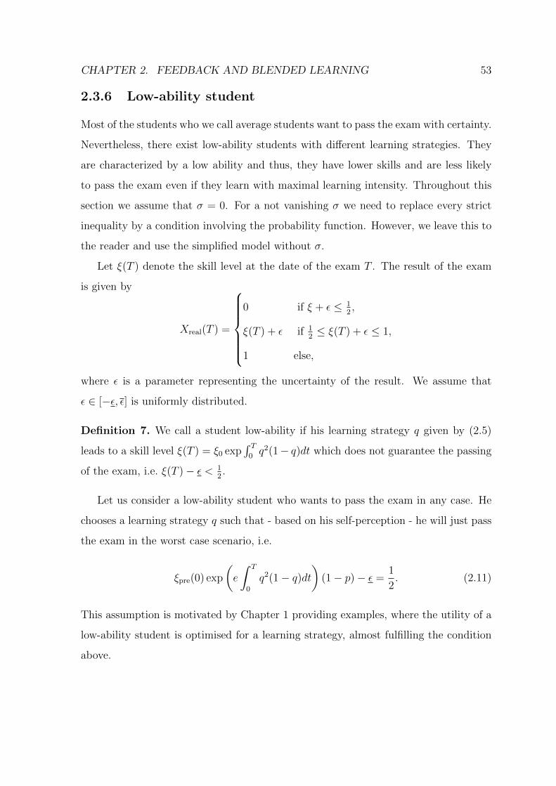
CHAPTER 2. FEEDBACK AND BLENDED LEARNING 53
2.3.6 Low-ability student
Most of the students who we call average students want to pass the exam with certainty.
Nevertheless, there exist low-ability students with different learning strategies. They
are characterized by a low ability and thus, they have lower skills and are less likely
to pass the exam even if they learn with maximal learning intensity. Throughout this
section we assume that σ = 0. For a not vanishing σ we need to replace every strict
inequality by a condition involving the probability function. However, we leave this to
the reader and use the simplified model without σ.
Let ξ(T ) denote the skill level at the date of the exam T . The result of the exam
is given by
Xreal(T ) =
0 if ξ + ε ≤ 1
2,
ξ(T ) + ε if 12≤ ξ(T ) + ε ≤ 1,
1 else,
where ε is a parameter representing the uncertainty of the result. We assume that
ε ∈ [−ε, ε] is uniformly distributed.
Definition 7. We call a student low-ability if his learning strategy q given by (2.5)
leads to a skill level ξ(T ) = ξ0 exp∫ T
0q2(1− q)dt which does not guarantee the passing
of the exam, i.e. ξ(T )− ε < 12.
Let us consider a low-ability student who wants to pass the exam in any case. He
chooses a learning strategy q such that - based on his self-perception - he will just pass
the exam in the worst case scenario, i.e.
ξpre(0) exp
(e
∫ T
0
q2(1− q)dt)
(1− p)− ε =1
2. (2.11)
This assumption is motivated by Chapter 1 providing examples, where the utility of a
low-ability student is optimised for a learning strategy, almost fulfilling the condition
above.
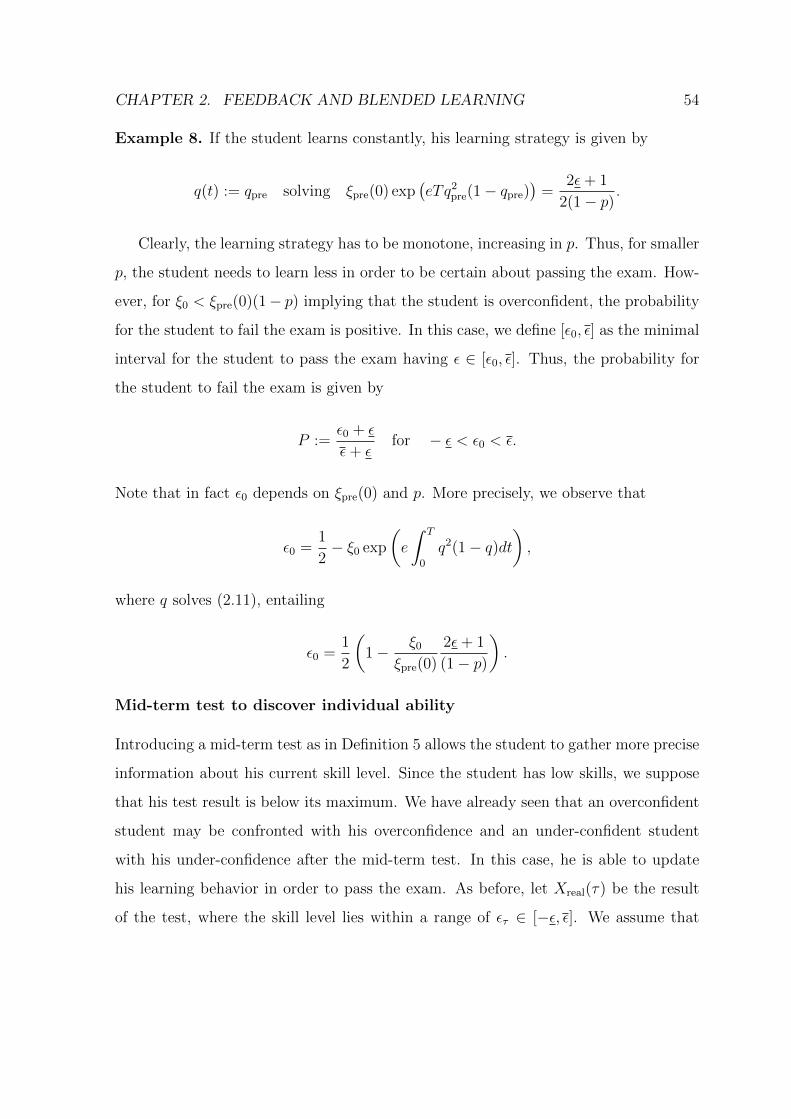
CHAPTER 2. FEEDBACK AND BLENDED LEARNING 54
Example 8. If the student learns constantly, his learning strategy is given by
q(t) := qpre solving ξpre(0) exp(eTq2
pre(1− qpre))
=2ε+ 1
2(1− p).
Clearly, the learning strategy has to be monotone, increasing in p. Thus, for smaller
p, the student needs to learn less in order to be certain about passing the exam. How-
ever, for ξ0 < ξpre(0)(1− p) implying that the student is overconfident, the probability
for the student to fail the exam is positive. In this case, we define [ε0, ε] as the minimal
interval for the student to pass the exam having ε ∈ [ε0, ε]. Thus, the probability for
the student to fail the exam is given by
P :=ε0 + ε
ε+ εfor − ε < ε0 < ε.
Note that in fact ε0 depends on ξpre(0) and p. More precisely, we observe that
ε0 =1
2− ξ0 exp
(e
∫ T
0
q2(1− q)dt),
where q solves (2.11), entailing
ε0 =1
2
(1− ξ0
ξpre(0)
2ε+ 1
(1− p)
).
Mid-term test to discover individual ability
Introducing a mid-term test as in Definition 5 allows the student to gather more precise
information about his current skill level. Since the student has low skills, we suppose
that his test result is below its maximum. We have already seen that an overconfident
student may be confronted with his overconfidence and an under-confident student
with his under-confidence after the mid-term test. In this case, he is able to update
his learning behavior in order to pass the exam. As before, let Xreal(τ) be the result
of the test, where the skill level lies within a range of ετ ∈ [−ε, ε]. We assume that

CHAPTER 2. FEEDBACK AND BLENDED LEARNING 55
the student overestimates his skill level, i.e. ξ(τ) < ξpre(τ)(1 − p). Thus, he realizes
his overconfidence if his test result is worse than predicted even in the most optimistic
view:
Xreal(τ) + ε < (1− p)Xpre(τ).
The probability that the student faces his own overconfidence with no doubt is therefore
given by ε1+εε+ε
with
ξ(τ) + ε1 + ε = (1− p)Xpre(τ).
Consequently, a mid-term test helps the low-ability student to update his true skill
level and to reflect his learning strategy. The knowledge about his current skills has
two effects. On one hand, his skills are lower than predicted and thus his learning
productivity is lower. This leads to decreasing incentives. If, on the other hand, this
leads to a positive probability of failing the test, the incentives could either increase or
lead to a complete dropout.
Finally, the probability to fail the exam is calculated by
Pnew :=(ε0 + ε)(ε− ε1)
(ε+ ε)2
=1 + 2ε
2(ε+ ε)2
(1− ξ0
ξpre(0)
1
(1− p)
)2
(1− p)ξpre(τ)
whenever it belongs to [0, 1], where
(1− p)ξpre(τ) =1 + 2ε
2exp
(−e∫ T
τ
q2(1− q)dt)≤ 1 + 2ε
2.
according to (2.11). Comparing this to the case without mid-term test shows
Pnew = P 2 exp
(−e∫ T
τ
q2(1− q)dt)≤ P 2
since P = 1+2ε2(ε+ε)
(1− ξ0
ξpre(0)2ε+1(1−p)
).

CHAPTER 2. FEEDBACK AND BLENDED LEARNING 56
This comparison emphasizes the reduction of the probability to fail the exam as a
result of participating in the mid-term test. If we assume an initial probability to fail
the exam of 50%, taking the mid-term test decreases this probability to less than 25%.
Consequently, a mid-term test is able to reduce the failure rate.
Dropout rate
Since low-ability students face a risk of failing the exam, dropping out of the exam can
be a better choice than learning in vain. In the following we will have a closer look at
the trade-off between learning and giving up.
For this, let us consider a low-ability student who is highly overconfident. Thus,
his real skill level is quite low compared to his individually estimated skill level:
ξ0 � ξpre(0).
Thereby, ξpre(0) is his estimated skill level at t = 0. We consider a student who,
according to his prediction, chooses a learning strategy with the aim to pass the exam
in the worst case scenario. However, he learns too little since he is highly overconfident.
Therefore, it is possible that the student has already no chance to pass the final exam
with certainty at the date of the mid-term test even if he continues to learn at maximal
intensity until the end of the semester. In this case, the optimal strategy for the student
might be, to stop learning and drop out of the course. Here, the mid-term test may
serve as a signal for the student to give up.
Let Xpre(τ) denote the predicted mid-term test result and p > 0 such that the stu-
dent assumes that his true skill level at time τ lies within the range [(1−p)Xpre(τ), (1+
p)Xpre(τ)]. The student therefore chooses the learning strategy qpre so that his learning
progress satisfiesξ(T )
ξ(τ)=
0.5 + ε
(1− p)Xpre(τ).
Note that here ξ(T ) depends on his actual learning strategy q = qpre. However, the

CHAPTER 2. FEEDBACK AND BLENDED LEARNING 57
actual skill level of the student at time τ is given by
ξ(τ) = ξ0 exp
(e
∫ τ
0
qpre(t)2(1− qpre(t))dt
), (2.12)
which leads him unavoidably to fail the exam if
ξmax(T, ξ) = ξ exp
(4
27e(T − τ)
)<
1
2− ε. (2.13)
for ξ = ξ(τ). Here, ξmax(T, ξ) denotes the maximal possible skill level at the time of
the exam under the condition that the student’s skill level at time τ is given by ξ. It
can be computed using the maximal learning strategy q = 23. This highly overconfident
student discovers his inability to pass the exam after writing the mid-term test if the
condition in (2.13) is fulfilled for every
ξ ∈ [Xreal(τ)− ε,Xreal(τ) + ε].
Thus, the probability that this student learns about his hopeless situation can be
computed by
P = max
{ε0 + ε
ε+ ε, 1
}for ε0 given by
(ξ(τ) + ε0 + ε) exp
(4
27e(T − τ)
)=
1
2− ε.
where ξ(τ) is given by (2.12). Consequently, the highly overconfident student gives up
and stops learning if this case occurs.
Within this section dealing with the decision-making of low-ability students, four
hypotheses summarize the main findings:
Hypothesis 3. If a low-ability student passes the mid-term test with an average result,
he will continue to learn unchanged.
Hypothesis 4. If a low-ability student passes the mid-term test with a better result,

CHAPTER 2. FEEDBACK AND BLENDED LEARNING 58
0.2 0.25 0.3 0.35 0.40
5
10
Xpre(τ)
rela
tive
uti
lity
chan
gein
%
0.2 0.25 0.3 0.35 0.4
2.3
2.4
2.5
·10−2
Xpre(τ)
uti
lity
Optimal qq based on self-perception
q optimized by mid-term test
Figure 2.2: Graph of the expected utility as a function of Xpre(τ) ∈ [0.2, 0.4] in thecase of ungraded exams. The figure shows the optimal case that the mid-term testresult coincided with the actual skill level with parameters given by T − τ = 2, e = 1,δ = 1
2log 2, γ = 1/6e−δT , ξ(τ) = 1
3, ε = ε = 0.1, p = 1
2and ετ = 0.
he will increase learning activity.
Hypothesis 5. If a low-ability student performs badly in the mid-term test, he will
learn more if and only if he has to recover to pass the exam.
Hypothesis 6. If a low-ability student who is highly overconfident performs very badly
in the mid-term test, he will give up and stop learning.
2.3.7 Ungraded exams
Ungraded exams can be found in many real-world settings, like in teacher-training
courses. Therefore, students face two possible outcomes: passing or failing the exam.
In order to analyze the impact on utility maximization for this case, we introduce a
different model of examination where final exams are not graded. As before, mid-term
tests remain graded. Thus, we assume that the results are given by
X(T ) =
1 if ξ(T ) + ε ≥ 12,
0 else.

CHAPTER 2. FEEDBACK AND BLENDED LEARNING 59
Similarly as above, ε ∈ [−ε, ε] is a parameter modeling unpredictable influences, which
is assumed to be uniformly distributed. The utility function is given as in (2.2). With-
out knowing the parameter ε exactly, the student is rather interested in the expected
utility. For −ε ≤ ξ(T )− 12≤ ε, it is approximately given by
Eu = e−δT2Eξ(T )− 1 + 2ε
2(ε+ ε)− γ
∫ T
0
qe−δtdt.
In case of an ungraded exam, we assume that the range [−ε, ε] is rather big such that
−ε ≤ ξ(T ) − 12≤ ε is probably satisfied for average students. Thus, throughout this
section, we will assume that the probability for the counter case is neglectable.
Likewise to Section 2.3.3, we suppose that the student has an imperfect knowledge
about his true skill level and is only able to predict it within the range [(1−p)ξpre(0), (1+
p)ξpre(0)]. Observing that the expected utility function is an affine transformation of the
one in Section 2.3.3, we can similarly compute the student’s optimal learning strategy.
Moreover, introducing a mid-term test at time τ = T2, the student is able to adapt
his learning strategy to qnew being the solution of
qnew(t)(2− 3qnew(t))ξnew(τ)
ε+ εexp
(∫ T
τ
q2new(1− qnew)ds− δT
)= γe−δt for τ < t ≤ T,
where ξnew(τ) is given by (2.10). Finally, we are able to derive the students’ new
expected utility by
eδTEunew =ξ0
ε+ εexp
e τ∫0
q2pre(1− qpre)dt+ e
T∫τ
q2new(1− qnew)dt
+
2ε− 1
2(ε+ ε)− γ
τ∫0
e−δtqpredt+
T∫τ
e−δtqnewdt
.
In order to find out whether the new strategy dominates the previous one, we need

CHAPTER 2. FEEDBACK AND BLENDED LEARNING 60
0.2 0.25 0.3 0.35
0
5
10
Xpre(τ)
rela
tive
uti
lity
chan
gein
%
0.2 0.25 0.3 0.35
2.3
2.4
2.5
·10−2
Xpre(τ)
uti
lity
Optimal qq based on self perception
q optimized by mid-term test
Figure 2.3: Graph of the expected utility as a function of Xpre(τ) ∈ [0.2, 0.4] in thecase of ungraded exams. The figure shows the optimal case that the mid-term test isworse than the actual skill level with Xreal(τ) = ξ(τ)− 0.05. The parameters used forthis plot are T − τ = 2, e = 1, δ = 1
2log 2, γ = 1/12, ξ(τ) = 1
3, ε = ε = 0.1, p = 1
2
to investigate the relative change in expected utility
∆EuEu
:=Eunew − Eu
Eu.
On the left-hand side of Figure 2.2 we see the relative utility change as a function of
the predicted skill level Xpre(τ). Note that this figure assumes ετ = 0. Consequently,
the mid-term test reveals the true skill level without uncertainty. The relative utility
change decreases if the predicted skill level is near the real skill level. Therefore, utility
decreases if the predicted skill level is far away from its real value.
The right-hand side of Figure 2.2 shows utility if learning time is based on the
condition that it is optimal, that it is based on the self-assessment and that it is
updated after the mid-term test. Utility increases for higher values of the predicted
skill level. Here, utility is on its lowest level if learning time is based on a low predicted
skill level. Note that learning time is optimal if the predicted skill level is equal to the
real skill level. Assuming a flawed self-assessment, the student is able to increase his
utility if he updates his learning activity according to the results of the mid-term test.
Consequently, taking the exam, the student is able to increase his utility by updating

CHAPTER 2. FEEDBACK AND BLENDED LEARNING 61
his learning strategy. In contrast to this, utility stays on a low level if the student does
not take the test and maintains his low learning time.
In contrast to Figure 2.2, Figure 2.3 assumes ετ > 0. Therefore, the mid-term test
does not always reveal the real skill level. Not surprisingly, utility in the case of the
updated learning time after the mid-term test only approaches the utility maximum,
since the updated skill level is based on the uncertainty of the test situation. Still, a
student who takes the mid-term test and updates his learning activity is mostly able
to increase his utility. However, assuming the student’s self-perception which reflects
his actual skill level, i.e. Xpre(τ) = ξ(τ), the feedback of the mid-term test can lead
to a less optimal learning behavior and decrease the student’s utility if the test result
is better or worse than the actual skill level. This is possible since the test result also
depends on the concentration and luck-level. Nevertheless, this is only a minor case
and the relative utility change is rather small see Figure 2.3.
In conclusion, the analysis of the utility with and without mid-term test emphasizes
the positive impact of feedback. In most cases, students are able to increase their utility
if they update their learning activity according to the gained information about their
real skill level.
2.3.8 Outlook
Among all results we have derived six hypotheses which may be tested empirically.
Since our research focuses on a theoretical analysis, further empirical research may
follow.
Without knowing the student’s predicted skill level, it is not possible to make state-
ments about his under- or overconfidence. The introduction of a placement examination
at the beginning of the semester may serve as a measure to receive information about
the individual skill level. Based on the result of this placement examination, students
are able to build their self-assessment. In addition, the result of the placement exami-
nation categorizes students into low-ability and average students. Since Hypothesis 1

CHAPTER 2. FEEDBACK AND BLENDED LEARNING 62
and Hypothesis 2 deal with average students and Hypothesis 3, Hypothesis 4, Hypoth-
esis 5 and Hypothesis 6 deal with a low-ability students, this distinction is necessary.
Participating in the mid-term test, students have the opportunity to discover their
under- or overconfidence. The learning activity before and after the mid-term test can
be measured by considering the time spent on solving online exercises.
Hypothesis 1 says that an average student who discovers his under-confidence will
increase his learning activity. It is possible to test this hypothesis by looking at a stu-
dent whose mid-term test result is better than the result of his placement examination.
In this case he should increase his learning activity because of the gained motivation.
Hypothesis 2 implies that an average student who discovers his overconfidence, will
reduce his learning time. This hypothesis can be confirmed if the student performs
badly in the mid-term test, although he expected a higher skill level according to the
placement examination. Furthermore, after discovering his overconfidence he would
feel frustrated and because of that reduce his learning activity .
Hypothesis 3 implies that a low-ability student will continue to learn if the result of
his mid-term test is average. This hypothesis may be tested by looking at the learning
activity before and after the mid-term test of a low-ability student with an average
result.
Hypothesis 4 implies that a low-ability student will increase his learning activity if
the result of his mid-term test is better. This hypothesis may be tested by looking at
the learning activity before and after the mid-term test of a low-ability student with a
better result.
Hypothesis 5 says that a low-ability student will learn more if the result of his
mid-term test is bad. This hypothesis can be proved by observing the learning activity
before and after the mid-term test of a low-ability student with a bad result.
Finally, Hypothesis 6 implies that a low-ability student who is highly overconfident
and performs very badly in the mid-term test will give up and stop learning. It is
possible to prove this hypothesis by showing that a low-ability student with a bad

CHAPTER 2. FEEDBACK AND BLENDED LEARNING 63
mid-term test result does not take the exam or stops solving online exercises.
2.4 Conclusion
This paper has extended the simple model of learning by doing in the context of
university courses (see Chapter 1) by introducing the role of feedback. Exam outcomes
are the result of accumulated skills through learning during the semester. Thereby, the
offered blended learning opportunities enable a flexible and around-the-clock learning
activity. Nevertheless, learning time is limited due to the trade-off between leisure
and learning time. We introduce feedback with the aim to analyze its impact on
students’ flawed self-assessment. In this context, online exercises and mid-term tests
serve as sources of feedback to check the individual skill level. Students who use blended
learning are able to compare their expected skill level to the received feedback and may,
based on this comparison, update their learning behavior.
Considering feedback on solving online exercises, we show that a student is able
to determine his growth rate of skills if he constantly makes use of this source of
feedback. Although feedback on online exercises rather offers hints about the learning
improvement than on the actual skill level, it connects performance of online exercises
to the learning progress. Thus, it has a huge influence on the utility function.
Assuming a mid-term test as source of feedback, students who take the mid-term
test have the opportunity to compare their predicted to their real skill level. Neverthe-
less, the test does not exactly describe the current skill level because of unpredictable
influences like luck and concentration. Furthermore, the student assumes that his
predicted skill level falls within a certain range because he is not able to estimate it
precisely. Therefore, the student is overconfident if his true skill level is smaller than
the lower bound of this range and under-confident if his true skill level is higher than
the upper bound. Otherwise, the student has a well-calibrated self-assessment. Making
use of the gained knowledge about his true skill level, the student is able to update

CHAPTER 2. FEEDBACK AND BLENDED LEARNING 64
his learning strategy. However, depending on the range of his predicted skill level, it
is also possible that an over- or under-confident student does not discover his flawed
self-assessment. Furthermore, we show that high-ability students who enjoy learning,
are motivated to learn more and low-ability students who should learn more learn less.
This result may be explained by intrinsic motivation which influences the commitment
to learn. While intrinsically motivated students are willing to learn more, students
who are frustrated or perceive barriers reduce learning performance independent of the
result of the mid-term test.
Furthermore, we analyze the decision-making of a low-ability student whose skill
level does not guarantee to pass the exam. We are able to show that a mid-term
test helps the low-ability student to discover his true skill level and, based on this
information, to update his learning behavior by adjusting it upwards. This knowledge
increases his probability to pass the exam. Nevertheless, we also show that students
who perform badly in the mid-term test stop learning and do not take the exam. Hence,
low-ability students face a high risk of perceiving barriers to learning and give up as a
consequence.
In addition to improving the self-assessment of skills and reducing the failure rate,
feedback also has a positive influence on utility. If students take the mid-term test and
update their learning time according to the gained information about their real skill
level, they mostly increase their utility.
Concluding, we are able to show that online exercises and mid-term tests as sources
of feedback are able to improve flawed self-assessment, learning performance and to
reduce the failure-rate if students make use of them on a regular basis.

Chapter 3
Blended learning as response to
student heterogeneity
Yvonne Maria Braukhoff 1
1Department of Economics, University of Duisburg-Essen, 45117 Essen Germany. Email:[email protected]
65

CHAPTER 3. HETEROGENEITY AND BLENDED LEARNING 66
Abstract
These days the student body is characterized by a considerable hetero-
geneity. Thus, higher education has to cope with new demands concerning
heterogeneous students. This paper analyzes dimensions of student hetero-
geneity and corresponding measures in order to respond to these changes.
Furthermore, the higher education system comprising bachelor’s and mas-
ter’s degrees is analyzed by comparing the signaling power of different de-
grees by using Spence’s (1973) signaling model. In contrast to prior one-
signal-degrees, this more differentiating system enables students to choose
different levels of higher education degrees and thus takes into consider-
ation student heterogeneity. Nevertheless, entering higher education does
not always ensure a successful completion. Dropout rates in higher educa-
tion may be the result of wrong self-assessment, since signaling requires the
knowledge of one’s individual productivity and capabilities.
In order to implement interventions in the daily teaching routine, JACK
as an example of blended learning is presented as a response to faulty
self-assessment and the increasing heterogeneity of students. On the one
hand, the implementation of JACK in university courses meets the growing
demands of a heterogeneous student body through guiding self-study and
through flexibility of time and space. On the other hand, JACK helps
to correct flawed self-assessment with the aid of immediate feedback and
opportunities to repeat course contents.
Consequently, this paper analyzes dimensions of student heterogeneity
and, based on this analysis, proposes blended learning as a successful mea-
sure to adapt teaching routines.

CHAPTER 3. HETEROGENEITY AND BLENDED LEARNING 67
3.1 Introduction
These days, higher education is characterized by an increasing heterogeneity of stu-
dents (Hanft 2015). Besides traditional aspects of heterogeneity like skills, professional
experiences, social and cultural background, diversity has further dimensions. New
sources of heterogeneity are represented by a broader age span and by differences in
organizing self-study among students (Schulmeister et al. 2012). The homogeneous
university structures, teaching methods and courses with a huge number of students
are confronted with these heterogeneous student characteristics. Thus, higher edu-
cation has to cope with new demands caused by student heterogeneity. Until now,
initiated actions like receiving inspections and preparatory courses concentrate mainly
on the orientation phase of and access to higher education studies and do not take
teaching routines into account (Hanft 2015). Instead of transforming heterogeneity
into homogeneity, higher education might be forced to adapt course structures in or-
der to accept and accommodate heterogeneous students (Biggs and Tang 2011; Wildt
2001).
Within the framework of the Bologna process, the higher education system has been
restructured to bachelor’s and master’s degrees (EACEA 2012). In contrast to prior
degrees like the Diplom in Germany, this highly differentiating system enables stu-
dents to choose different levels of higher education degrees according to their cognitive
abilities and commitment level and therefore has to cope with a higher heterogeneity
within bachelor’s degrees. In addition, the Bologna process aims to harmonize tertiary
education among European countries. Under this common framework, bachelor’s and
master’s degrees have been standardized to improve the equivalence between similar
programs and to simplify students’ international mobility.
In this connection, the completed degree serves as a signal for the employer, which
reduces his uncertainty concerning the productivity of the graduate (Spence 1973). In
order to compare the signaling power of different degrees, I compare a one-signal-degree
and the bachelor’s and master’s degree as a two-signal-degree by using Spence’s (1973)

CHAPTER 3. HETEROGENEITY AND BLENDED LEARNING 68
signaling model.
Spence’s signaling model assumes students to be perfectly informed about their
skills, but entering higher education does not always ensure a successful graduation in
reality. Although the choice of bachelor’s and master’s degrees gives individuals differ-
entiated possibilities of education, many students drop out. According to the results
of the research of “OECD-Education at glance” (OECD 2013) and “Bologna Process
Implementation Report” (EACEA 2012), only 70% of students who enter higher edu-
cation graduate among OECD countries. This dropout rate in higher education may
be the result of faulty self-assessment, since signaling requires the knowledge of one’s
individual productivity.
With the aim of accepting student heterogeneity and improving the flawed self-
assessment, higher education should give more attention to the adaptation of course
structures instead of purely concentrating on the selection process before the start of
higher education studies. In order to implement actions in the daily teaching routine, I
propose blended learning as a response to the frequently imperfect self-assessment and
increasing heterogeneity of students.
Blended learning combines traditional face-to-face sessions with online learning op-
portunities which are available 24 hours per day and 7 days per week. E-learning
exercises take individual preferences and living conditions into account, since they are
characterized by a high flexibility of time and space. In addition, they help to organize
the self-study and improve the retention of acquired course contents. The immediate
feedback helps to validate acquired skills and to recognize one’s progress in learning.
Beside these advantages of blended learning, the current learning environment shows
a trend towards online learning. Many surveys confirm this trend by emphasizing
that online learning tools have significantly increased in students’ learning experiences
(Allen and Seaman 2006) and that students show a new attitude towards online learn-
ing (Sebastianelli and Tamimi 2011).
Thus, this paper analyzes dimensions of student heterogeneity, copes with the more

CHAPTER 3. HETEROGENEITY AND BLENDED LEARNING 69
heterogeneous educational offers and shows how differentiated and more flexible learn-
ing arrangements pay attention to these dimensions and improves a potentially flawed
self-assessment.
3.2 Student heterogeneity
3.2.1 Dimensions of student heterogeneity
Nowadays, higher education is characterized by an increasing heterogeneity among
students. This growing heterogeneity has multiple reasons. The first reason is caused
by the increasing number of first-year students. Over the past 16 years, the number of
graduates has increased by nearly 20 percent on average across OECD countries (OECD
2013). Furthermore, more than 50 percent of each age group start to study (OECD
2011). Looking at Germany, the number of first-year students doubled since the 80s
and 90s, having arrived at a higher overall count than beginners of apprenticeships
(Hanft 2015).
Secondly, universities are open to all social classes which had no opportunity to
study in former times. Thus, in these days higher education studies are not reserved
to the elites anymore (Middendorf 2015). Beyond this, our society is characterized
by a social change with a multitude of background conditions to grow up with. Con-
sequently, the student body shows an increasing age span and differences in regard
to previous experiences, skills, motivation, goals and social background (Middendorf
2015). In this context, some policy changes in Germany lead to younger first-year
students, while changing living conditions lead to older students. These are reasons for
the described age span. The educational reform G8, for instance, shortened the overall
duration of compulsory schooling by one year in Germany. In addition, conscription
has been discontinued, i.e. young men are not obligated to compulsory military ser-
vice anymore and thus begin to study earlier. Moreover, many students are gainfully
employed during their studies or work before or between their bachelor’s and master’s

CHAPTER 3. HETEROGENEITY AND BLENDED LEARNING 70
degree (Hanft 2015). This additional workload may lead to a postponed graduation
and an advanced age.
Alauddin and Ashman (2014) confirm these significant changes in the student body
over the last two decades by adding an international dimension. Beside the increased
number of students, the share of international students has expanded in particular.
This trend is confirmed by the OECD Indicators (2015) which emphasize that inter-
national students constitute a significant share of higher education graduates among
OECD countries. In more detail, it has been shown that 18% of students who attained
a master’s degree and 7% who attained a bachelor’s degree are international students.
The internationalization of higher education entails a highly diverse cultural back-
ground with individual differences in the philosophy of studying and learning (Johnson
and Kumar 2010). This philosophy is shaped by previous experiences at home like
expectations and pressure exerted by the family.
Beside traditional aspects like social background, age, skills and professional experi-
ence, diversity has further dimensions which go beyond the traditional ones. Schulmeis-
ter et al. (2012) emphasize a different learning behavior among students as new source
of heterogeneity. By analyzing how students spend their time on self-study, attending
courses and leisure time, they discover a wide range of time allocation leading to differ-
ent results. Although students face the same homogeneous university structures, every
student responds in a different manner of time management. The resulting diverse
learning behavior leads to different learning outcomes and university success. Espe-
cially the time spent on self-study is characterized by a huge diversity among students.
In contrast to this, the participation in courses is almost the same for all students. As
a response to the diversity of learning behavior, Schulmeister et al. (2012) demand
new teaching methods which support the organization and support of self-study.
As we have seen, student heterogeneity comprises many dimensions which provide
higher education with new challenges.

CHAPTER 3. HETEROGENEITY AND BLENDED LEARNING 71
3.2.2 Current measures to respond to student heterogeneity
Until now, initiated actions mainly concentrate on the introductory phase of higher
education studies and do not take account of teaching routines (Hanft 2015). Coun-
seling, tutorials and preparatory courses are offered in order to prepare students for
their studies and in order to select the appropriate individuals. However, a change of
university structures still has not yet been realized. Receiving inspections aim to create
homogeneous student groups. All these actions aim to homogenize the student body
without changing organization and structures of higher education. Thus, until now
homogeneous university structures persist and only the orientation phase attempts to
meet the requirements of the growing heterogeneity of students.
In this context, Wildt (2001) distinguishes two dimensions of measures. On the one
hand, heterogeneity may be accepted and the universities can respond to the changing
requirements. On the other hand, heterogeneity may be transformed into homogeneity.
As described above, higher education so far mainly focuses on transforming heterogene-
ity into homogeneity. However, the first aspect, accepting heterogeneity, shall be given
higher priority in the future, if the requirements of society are going to be met. This
point of view is also supported by Bigg and Tang (2011), who argue that university
teaching should be adapted to the needs of an increasingly heterogeneous student body.
Section 3.4 focuses on this gap by adapting course structures and thus, accepting het-
erogeneity. Before we cope with this aspect, we start with a simple signaling model
analysing the changing incentives with more differentiated educational programmes.
3.3 The signaling mechanism in higher education
The choice between differentiated higher education degrees is one possibility to cope
with higher heterogeneity of students. Certificates in higher education like the bache-
lor’s and the master’s degree do not only represent an investment in education, they also
serve as a signal for the employer in case of otherwise asymmetrical information. This

CHAPTER 3. HETEROGENEITY AND BLENDED LEARNING 72
section analyzes the signaling mechanism of degrees in higher education and compares
their signaling power with respect to student heterogeneity.
3.3.1 Theoretical background
In 1973, Spence introduced the aspect of education as a signaling device on the job
market for the first time. Since asymmetrical information prevails on the job market,
the employer would like to learn about the productivity of the individual before hiring
him. In order to counteract this uncertainty, according to Spence individuals have
the opportunity to invest in education involving costs in terms of money and time
which vary according to the individual skills. Obtaining a degree serves as an observ-
able signal for the employer if skills and productivity are correlated. Consequently,
in this context education can be a signal to reduce the inefficiencies associated with
asymmetric information.
Spence (1973) distinguishes two groups of high and less productive individuals who
are assumed to know their own skills. Every individual can choose to specifically invest
in education. Signaling works, if costs are negatively correlated with individual skills
and productivity, since highly productive individuals then have lower costs to reach a
specific education level than low-ability individuals.
In equilibrium then a critical level of education y∗ exists which distinguishes high
and less productive individuals. According to this wage schedule, individuals choose
their investment in education with the aim to maximize their utility, given by the
difference between wage and signaling-costs. In a signaling equilibrium, high-ability
individuals invest the critical level of education y∗, while low-ability individuals do not
invest in education.
Thereby, the employer pays a wage according to education level, even if education
has no impact on skills and thus on productivity. It is pure self selection that makes
differences in wages and job offers. If employers are completely competitive, wages
paid in equilibrium equal expected individual productivity.

CHAPTER 3. HETEROGENEITY AND BLENDED LEARNING 73
In this equilibrium, there exists overinvestment in education, even if education has
a positive impact on skills and productivity. There are also pooling equilibria without
signalling. This is however in general instable if employers have credible beliefs about
the equilibrium path. If signaling cost are high and the share of high skill workers is
low, the pooling equilibrium dominates the separating equilibrium however.
Spence assumed a continuous spectrum of educational levels. In practice however
there are only specific degrees. This might be unable to cope with larger or increasing
heterogeneity. With only one specific degree, in Germany the Diplom, full separa-
tion would not be possible. Differentiating the degrees by splitting the Diplom into
bachelor’s and master’s degrees allows to further differentiate the different skill level.
The following subsection analyses the different equilibria and asks, which group
might be better off after the change and which group might be worse off.
3.3.2 Signals in higher education
Certificates in higher education like the bachelor’s, the master’s degree and the German
Diplom represent an investment in education incurring costs, which allows students to
distinguish themselves from less productive individuals by choosing a specific degree.
If different talented students behave in a different manner according to their individual
ability the chosen degree might serve as a signal for the employer and determine the
individual wage.
An investment in higher education bears the possibility to indicate that students are
able to learn sizeable quantities over a longer period of time, that they are able to pass
exams, that they can work in a team, that they function in a social setting and that they
are able to follow a predetermined schedule (Krassen 2014). Consequently, investing
in higher education represents the acquisition of skills and the ability to achieve a
goal. Obtaining a higher education degree serves as a signal if students reveal their
ability depending on their graduation. Although signals give no information about
the student’s ability to do the job, they show to which extent the student invested

CHAPTER 3. HETEROGENEITY AND BLENDED LEARNING 74
effort and costs. Since the labor market is characterized by asymmetric information,
costly signals offer a remedy to the resulting inefficiency by resolving asymmetries
of information. Nevertheless, there is a risk of over-education which may result in
the distortion of the signal and the bumping-down effect on less educated people. If
more and more students complete higher education degrees, the pressure to further
increase higher education arises. This situation is not desirable because the degree as
a signal loses its power. Therefore, higher education should give better opportunities
to differentiate.
In this connection, the switch to the system of bachelor’s and master’s programs
offers more differentiating opportunities for students of higher education, in contrast
to prior one-signal-degrees like the Diplom in Germany. The resulting offer of different
degrees may reduce over-education.
In order to analyze different higher education degrees and its signaling power, I
extend Spence’s signaling model from 1973 by introducing a third level of productivity.
Since nowadays higher education is characterized by a differentiated system of degrees
comprising bachelor’s and master’s degrees, the model needs differentiated equilibrium
cut off levels. In order to emphasize the signaling power of the bachelor’s and master’s
degrees in contrast to the signaling power of the Diplom as a one-signal-example, I use
a numerical example.
I assume three groups of individuals with different productivity levels θ. Individuals
of Group 1 (low ability) have a productivity of θl = 1 and signaling costs of cl = y,
individuals of Group 2 (mid ability) are characterized by a level of productivity of
θm = 2 and signaling costs of cm = y2
and finally, individuals of Group 3 (high ability)
show a level of productivity of θh = 3 and signaling costs of ch = y3. Population shares
of the three groups are given by: ql, qm and qh = 1− ql − qm.
In the case of Bologna including bachelor’s and master’s degrees, the employer takes
two critical levels of education yB and yM into consideration which distinguish high-
, mid- and low-ability individuals. Consequently, if y < yB in equilibrium expected

CHAPTER 3. HETEROGENEITY AND BLENDED LEARNING 75
productivity equals 1, if yB ≤ y < yM expected productivity equals 2 and if y ≥ yM
expected productivity equals 3. In this case, there are three in equilibrium values of y:
y = 0, y = yB and y = yM .
In a signaling equilibrium, individuals of Group 1 set y = 0 if
1 ≥ 2− yB.
Individuals of Group 2 set y = yB if
1 ≤ 2− yB
2,
and do not choose y = yM if
2− yB
2≥ 3− yM
2.
Finally, individuals of Group 3 set y = yM if
2− yB
3≤ 3− yM
3.
The levels of education have to satisfy the following inequality:
1 < yB < 2 < yM − yB < 3.
For further calculation I focus on the efficient critical levels of education which are
given by
yB = 1 and yM = 3.
These education levels do not reflect academic years but required effort and level of
difficulty of the degree. In contrast to the bachelor’s degree which implies three years of
studies and the acquisition of basic knowledge, the master’s degree includes two years
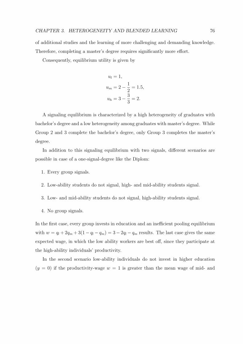
CHAPTER 3. HETEROGENEITY AND BLENDED LEARNING 76
of additional studies and the learning of more challenging and demanding knowledge.
Therefore, completing a master’s degree requires significantly more effort.
Consequently, equilibrium utility is given by
ul = 1,
um = 2− 1
2= 1.5,
uh = 3− 3
3= 2.
A signaling equilibrium is characterized by a high heterogeneity of graduates with
bachelor’s degree and a low heterogeneity among graduates with master’s degree. While
Group 2 and 3 complete the bachelor’s degree, only Group 3 completes the master’s
degree.
In addition to this signaling equilibrium with two signals, different scenarios are
possible in case of a one-signal-degree like the Diplom:
1. Every group signals.
2. Low-ability students do not signal, high- and mid-ability students signal.
3. Low- and mid-ability students do not signal, high-ability students signal.
4. No group signals.
In the first case, every group invests in education and an inefficient pooling equilibrium
with w = ql + 2qm + 3(1− ql− qm) = 3− 2ql− qm results. The last case gives the same
expected wage, in which the low ability workers are best off, since they participate at
the high-ability individuals’ productivity.
In the second scenario low-ability individuals do not invest in higher education
(y = 0) if the productivity-wage w = 1 is greater than the mean wage of mid- and

CHAPTER 3. HETEROGENEITY AND BLENDED LEARNING 77
high-ability individuals minus education costs according to the following equation:
1 ≥ 3− 3ql − qm1− ql
− y.
As a consequence, low-ability students earn wl = 1 and mid- and high-ability graduates
earn the mean wage w2/3 = 3−3ql−qm1−ql
and the critical level of education equals y∗ =
2−2ql−qm1−ql
.
In this case, utility is given by
ul = 1,
um =4− 4ql − qm
2(1− ql),
uh =7− 7ql − 2qm
3(1− ql).
Highly productive individuals lose because they earn less, while mid-ability individuals
win and make a profit of the mean productivity.
Finally, in the third case I assume that only high-ability students invest in education
and complete the Diplom, while low- and mid-ability individuals set y = 0. Therefore,
the following inequality holds
ql + 2qmql + qm
≥ 3− y
2.
Consequently, low- and mid-ability students earn the mean wage wl/m = ql+2qmql+qm
and
high-ability graduates earn wh = 3 and the critical level of education equals y∗ =
6− 2(ql+2qm)ql+qm
= 2(2ql+qm)ql+qm
.

CHAPTER 3. HETEROGENEITY AND BLENDED LEARNING 78
Therefore, utility is given by
ul =ql + 2qmql + qm
,
um =ql + 2qmql + qm
,
uh =5ql + 7qm3(ql + qm)
.
In this case high-ability individuals are payed according to their productivity. Low-
ability individuals benefit from the mean wage, while mid-ability individuals lose.
Consequently, if I assume three productivity-level and only one signal, not every
individual is payed according to his productivity. Every possible situation includes a
mean wage which puts some individuals at a disadvantage and others at an advantage.
Therefore, every equilibrium includes winners and losers.
Practical application
In order to illustrate the derived outcomes, I introduce examples for a particular case
and calculate the critical level of education and individual utility for the three described
scenarios.
For this purpose I apply the results of the survey “OECD-Education at glance”
(2015). According to this survey, an average of 36% of populations in OECD countries
received a bachelor’s degree, while about 17% received a master’s degree in 2013. Since
I assume that high-ability individuals are able to complete the master’s degree and mid-
ability individuals the bachelor’s degree, I assume for reasons of simplicity the following
population-shares: ql = 0.5, qm = 0.4, qh = 0.1.
Thus, in the first case assuming these population-shares a pooling equilibrium with
ui = wi = 1.6 results. Since many students graduate with a degree, this equilibrium
can be neglected.

CHAPTER 3. HETEROGENEITY AND BLENDED LEARNING 79
In the second scenario, mid and high-ability students graduate with a Diplom and
y = 1.2; ul = 1; um = 1.6; uh = 1.8.
Finally, if only high-ability students finish their studies with a Diplom, the following
outcomes result
y = 3.12; ul = um = 1.44; uh = 1.96.
In this context, descriptive statistics prove that graduates with a Diplom as degree
earn on average 7200 Euro more per year than graduates with a bachelor’s degree
(Briedis and Minks 2005). This wage differential among graduates indicates a higher
productivity among Diplom graduates in contrast to Bachelor’s graduates. Thus, the
third scenario in which only highly productive individuals signal appears to be an
accurate depiction of reality. If no wage differential between bachelor’s and Diplom
graduates existed the second scenario would be more realistic.
After checking the relevance of the practical application for all scenarios, I am now
able to compare the relevant two scenarios: the signaling equilibrium with bachelor’s
and master’s degrees and the signaling equilibrium with high-ability individuals com-
pleting a Diplom.
In case of a signaling equilibrium with bachelor’s and master’s programs, mid- and
high-ability individuals benefit in comparison to a signaling equilibrium with Diplom,
in which only high-ability individuals signal. Since high-ability individuals have to put
a distance between themselves and low- and mid-ability individuals, the critical level
of education is higher in case of a Diplom. Consequently, their utility is less than
their utility with a master’s degree. In addition, mid-ability individuals do not have
the opportunity to signal, meaning that their utility equals the mean wage of low-
and mid-ability graduates which is less than their utility with a bachelor’s degree. In
contrast to this, low-ability individuals benefit from this mean wage which is greater

CHAPTER 3. HETEROGENEITY AND BLENDED LEARNING 80
than their wage in case of the signaling equilibrium with bachelor’s and master’s de-
grees. Consequently, the signaling equilibrium with bachelor’s and master’s degrees
represents an improvement for high- and mid-ability individuals and a deterioration
for low-ability individuals.
In order to confront these results with an example with differentiating levels of pro-
ductivity, I take actual wage differentials into consideration. Among OECD countries,
people with a higher education degree are characterized by an advantage in earnings.
Relative earnings rise with educational attainment. Thereby, higher education gradu-
ates can expect to earn 60 % more than people with non-tertiary education (OECD
2015). In addition, according to the salary survey of the National Association of
Colleges and Employers (NACE 2013) and according to the survey of Bispinck et al.
(2012), in many career areas the starting salaries of master’s graduates are about 20%
higher than the starting salaries of bachelor’s graduates.
Thus, in order to improve the practical orientation of the model, I adapt the val-
ues of the productivities of the three groups. The levels of productivity are changed
according to the described and empirically proved wage differentials.
Since wage is equal to productivity, I assume that low-ability individuals are charac-
terized by a productivity of θl = 1, mid-ability individuals of θm = 1.6 and high-ability
individuals of θh = 1.9, taking wage differentials into account. Signaling costs, popu-
lation shares and previously derived assumptions remain unchanged.
In the case of a signaling equilibrium with two signals representing bachelor’s and
master’s degrees, the critical levels of education are
yB = 0.6 and yM = 1.2
and utility is given by
ul = 1;um = 1.3;uh = 1.5.
CHAPTER 3. HETEROGENEITY AND BLENDED LEARNING 81
If no signal exists, a pooling equilibrium with ui = wi = 1.33 results for all individuals.
Furthermore, in the second scenario there exists only one signal and mid- and high-
ability individuals signal. Here, the critical level of education is y = 0.66, leading to
the following values of utility
ul = 1; um = 1.33; uh = 1.44.
Finally, in the case of only one signal when high-ability individuals invest in education,
the critical education level is y = 1.26 and utility is given by
ul = um = 1.27; uh = 1.48.
Now I compare the relevant two scenarios in the case of the adapted levels of produc-
tivity: the signaling equilibrium with bachelor’s and master’s degrees and the signaling
equilibrium with high-ability individuals completing a Diplom.
In case of a signaling equilibrium with bachelor’s and master’s graduates, the high-
and mid-ability individuals benefit while low-ability individuals lose in comparison to
the one-signal equilibrium. Since low-ability individuals are payed according to their
productivity instead of the mean-productivity, they lose. In contrast to this, mid-
ability individuals have the possibility to distinguish themselves through a bachelor’s
degree and thus they are able to obtain a greater wage. High-ability individuals have
to invest less in education in case of a master’s degree. In case of a Diplom, high-ability
individuals have to put a distance between themselves and low- and mid-ability indi-
viduals. Therefore, in this case the critical level of education is higher. Consequently,
the bachelor’s and master’s degrees lead to an improvement for high- and mid-ability
individuals and to a deterioration for low-ability individuals.
Although I have adapted levels of productivity according to empirically-proved
wage differentials, the results remain the same. Utility varies according to the wage
differentials but winners and losers remain the same.

CHAPTER 3. HETEROGENEITY AND BLENDED LEARNING 82
On the one hand, I am able to emphasize that the bachelor’s and master’s system
leads to an increase of utility for high- and mid-ability individuals because they are
paid according to their productivity. On the other hand, I show that utility of low-
ability individuals decreases, since they do not benefit anymore from the mean wage.
In contrast to this, a Diplom leads to a very high investment in education because
high-ability individuals have to distinguish themselves from the other two groups. In
addition, low-ability individuals earn more and mid-ability individuals earn less than
they contribute to the firm. Thus, a system with two signals is much more suitable to
reduce asymmetrical information in comparison to a system with only one signal.
3.3.3 Self-assessment and dropout rate of students
Although the bachelor’s and master’s system enables individuals to choose an adequate
degree, entering higher education does not always ensure successful graduation. Ac-
cording to the results of the research of “OECD-Education at glance” (OECD 2013)
and “Bologna Process Implementation Report” (EACEA 2012), only 70% of the stu-
dents who enter higher education graduate among OECD countries.
The students who do not complete their studies drop out. Thereby, dropout may
have various reasons and motivations. On the one hand, students may drop out of uni-
versity because the study program does not fit their interests, expectations or knowl-
edge, or because they find an attractive employment opportunity. On the other hand,
the higher education system may not meet their needs (OECD 2013).
The individual self-perception of ability might be a reason why university require-
ments and perceived knowledge do not fit and thus cause notable dropout. This paper
focuses on flawed self-perception as a reason for dropout. Self-perception of ability
plays a crucial role in the decision to invest in higher education, the choice of degree
and the probability of graduation. On the one hand, underestimation may prevent en-
rollment and reduce success. On the other hand, overestimation may lead to dropout
and disappointment. Especially overconfident individuals are more risky and there-

CHAPTER 3. HETEROGENEITY AND BLENDED LEARNING 83
fore may fail more often than well-calibrated individuals (Barber and Odean 2001).
Moreover, the “hard-easy effect” proves that individuals are overconfident concerning
their abilities when they are confronted with a difficult task and underconfident be-
ing confronted with an easy task (Lichtenstein and Fischhoff 1977; Benoıt and Dubra
2011).
In contrast to over- and underconfident students, March et al. (2005) make use of
longitudinal data in order to show that students with a good self-concept show a more
efficient allocation of study time and achieve better university outcomes. Thus, the
authors emphasize the positive influence a good self-perception may exert.
A wide range of literature examines the self-perception of students and its impact
on their studies. In this context, Chevalier et al. (2009) investigate the impact of
students’ self-perception on participation rates in higher education and find out that
students misconceive their own performance and especially over-estimate their own
ability. Thereby, a high self-perception supports the decision to attend higher educa-
tion. The dimension of these effects varies according to class and gender gaps.
Furthermore, by examining self-assessment in real-world settings, Dunning et al.
(2004) show that most students are not able to self-assess themselves accurately and
even tend to be overconfident concerning acquired skills. Moreover, students are often
not able to assess whether they have understood newly acquired skills because they
focus on the quick acquisition of contents and neglect and underestimate the retention
and the transfer of course contents. For this reason, authors propose feedback as an
opportunity to improve pupil’s self-assessment and check newly acquired contents, since
feedback helps students to judge their own performance.
In addition, quantitative self-assessment studies which compare self-assessed grades
and teacher grades in higher education show that the correlation between these grades
is higher in advanced classes in contrast to introductory classes (Falchikov and Bound
1989). If I interpret the correlation of grades as a measure of correct self-perception,
experience has a positive influence on self-assessment. Consequently, in contrast to

CHAPTER 3. HETEROGENEITY AND BLENDED LEARNING 84
students of introductory classes, the students of advanced classes are more experienced
and therefore are able to self-assess themselves more precisely.
On the one hand, an extended offer of opportunities to repeat course contents
might help students to acquire experiences in solving exercises and thus improve self-
perception. On the other hand, feedback may be another solution to the flawed self-
perception of students. Receiving feedback enables students to check and to update
their self-assessment. In addition, repetition and feedback are means to pay attention
to students’ needs.
3.4 New measures as response
Section 3.2.2 has described current measures to respond to student heterogeneity. These
actions mainly concentrate on the start of higher education studies and take no account
of teaching routines. By taking reasons for dropout into account, Section 3.4 presents
blended learning as a measure which is implemented in the daily teaching routine
and may be a response to the flawed self-assessment and increasing heterogeneity of
students.
3.4.1 Blended learning as response
As a response to the growing heterogeneity of students, Schulmeister et al. (2012)
demand new teaching reforms which support students’ self-study which is neglected in
traditional teaching methods. In addition to face-to-face sessions, they need support,
feedback and extra exercises to guide their self-study. Newly acquired knowledge has to
be consolidated through application. If students have the possibility to apply and re-
peat course contents and if they receive feedback during this repetition, self-assessment
and individual motivation may be increased.
In this context, online exercises may be a response to this heterogeneity since they
offer different levels of difficulty and are available 24 hours per day during 7 days per

CHAPTER 3. HETEROGENEITY AND BLENDED LEARNING 85
week. Solving exercises represents a repetition and consolidation of acquired knowledge
and entails feedback after entering a solution. Furthermore, students are free to choose
how often and on which exercises they work.
Beside the advantages of online exercises, the current learning environment is char-
acterized by a trend towards online learning. This is the reason why blended learning
begins to take the place of traditional teaching methods. This trend is confirmed by
various surveys that show that online learning tools in students’ learning experience
have increased significantly (Allen and Seaman 2006) and that students show a new
attitude towards online learning (Sebastianelli and Tamimi 2011). In Germany, for
example, nearly every university offers an e-learning platform (Henning 2015). How-
ever, the virtual learning environment places new demands on educators (Harasim et
al. 1995). Beside the traditional requirements, guiding and helping students through
formative feedback becomes more important. Attending to feedback, students are able
to self-regulate their learning activity. Thereby, self-regulated students are able to
estimate their own skills and to update and organize their further learning activities
(Butler and Winne 1995). In the context of computer-supported learning, Zumbach
and Reimann (2003) confirm the positive influence of external feedback on students’
motivation and problem-solving.
As a response to the heterogeneity of students, blended learning offers extensive
possibilities to repeat course contents and it offers guided learning and feedback. Con-
sequently, the described advantages of blended learning might meet the requirements
of heterogeneous students and serve to improve the flawed self-assessment.
3.4.2 JACK as example for blended learning
Description of JACK
JACK was developed and is provided by PALUNO (The Ruhr Institute for Software
Technology) and represents a computer-aided system offering online exercises and their

CHAPTER 3. HETEROGENEITY AND BLENDED LEARNING 86
automatic assessment and grading (Goedicke et al. 2008). Teachers have the opportu-
nity to generate multiple-choice and fill-in exercises. Thereby, JACK does not correct
longer proofs and text sequences and thus is particularly suitable for sciences related to
mathematics. Students are free to submit answers without time restriction and receive
an immediate evaluation by the feedback-function of JACK. Randomized variables are
used for every online exercise in order to offer a variety of opportunities to repeat
course contents and in order to confront every student with different exercises. Access
to JACK is provided to students which sign in with their matriculation number. Each
user account contains information about solved exercises and their evaluation. Online
tests are administrated on a different platform and their grading is published with a
delay.
This section focuses on the courses in microeconomics of the Chair of Microeco-
nomics at the University of Duisburg-Essen which use JACK as online tool. Beside of-
fering weekly lectures and tutorial classes as usual, JACK is implemented as e-learning
setting. While weekly lectures and tutorial classes aim to teach basic knowledge and
demonstrate examples, the e-learning opportunities offered by JACK represent a pos-
sibility of around-the-clock self-training and assessment of course contents. Since the
courses in microeconomics combine face-to-face sessions and e-learning opportunities,
blended learning is applied.
The courses in microeconomics are characterized by a considerable number of stu-
dents. Face-to-face sessions are visited by about 800 students while about 600 students
take part in the final exam at the end of the semester. This huge student body places
new demands on teachers. Here, JACK provides a measures of support. On the one
hand, students have the opportunity to solve online exercises around-the-clock and on
the other hand they can participate in a mid-term test with the aim to improve the
final exam mark.
Every topic of the course is accompanied by various online exercises for the purpose
of self-study. These exercises have the form of multiple-choice or fill-in tasks. Thereby,

CHAPTER 3. HETEROGENEITY AND BLENDED LEARNING 87
each student receives the same task but different numbers since variables are random-
ized. After solving the exercise by entering a numerical solution or marking with a
cross, the student immediately gets a feedback whether his answer was partially or
completely faulty or correct. In the case of a wrong answer the student has the pos-
sibility to repeat the exercise, to get a hint by pressing the hint-putting, or to obtain
the solution. Exercises have several stages with increasing level of difficulty. Thus, in
the case of the right answer or obtaining the solution, the student is guided to the next
stage.
With the aim to avoid last-minute learning and to increase commitment, online mid-
term tests with the possibility to gain bonus points for the final exam are also offered.
The existence of a mid-term test enhances students’ engagement in early learning and
the seriousness of early learning. Thereby, students are free to choose whether they
take part or not. A failed mid-term test has no negative effect. If the student passes
the test, he gains bonus points which improve his final exam mark. Nevertheless, bonus
points are only credited if the student passes the exam without bonus points. Thus,
bonus points do not help to pass the exam but to improve the mark.
The key advantage of online tests lies in their fairness and the immediate electronic
correction. Online tests have a substantially reduced workload of correction and are
objective since correction is automatic, whereas correction by hand varies among differ-
ent teachers and depends on the individual concentration and form on the day. Since
the mid-term tests are offered online, students may solve them at home. Although they
can work in groups or use documents and books, every student obtains randomized and
therefore individualized numbers.
Consequently, the described courses in microeconomics are characterized by an
extensive offer of blended learning. While weekly lectures and tutorial classes teach
course contents, online exercises guide the self-study and mid-term tests entail the
possibility to improve the final exam grade.

CHAPTER 3. HETEROGENEITY AND BLENDED LEARNING 88
JACK’s contribution
In consideration of the dimensions of student heterogeneity described in Section 3.2.1
and with regard to the flawed self-assessment described in Section 3.3.3, I now empha-
size the contribution of JACK.
Since the number of first-year-students has increased significantly, courses are vis-
ited by a considerable number of students. Therefore, teachers are not able to guide
students individually. JACK has the possibility to pay attention to every student by
offering a huge number of exercises which repeat course contents. In addition, every
student receives individual feedback after the submission of a solution.
Since universities are open to all social classes, financing of studies represents a
burden for students of low-income families. In this connection, e-learning offers a
variety of learning opportunities which are free of charge.
Furthermore, many students are gainfully employed during their studies and show
differences in the organization of their daily life. Since online exercises are available
around-the-clock and since they can be solved everywhere, they offer a high flexibility
of time and place. This flexibility enables students to learn according to their individual
preferences of time. Flexibility and different levels of difficulty are also means to pay
attention to international students with different cultural background.
In addition, the diversity of individual learning behavior and especially the orga-
nization of self-study is described as a new source of student heterogeneity. Applying
JACK, students start solving exercises at the beginning of the semester and maintain
this effort on self-study during the whole semester, instead of learning mainly at the
end of the semester before the final exam. Thus, the possibility to learn around-the-
clock represents an incentive to learn on a regular basis during the semester. Thereby,
overall learning time is higher than usual before the mid-term test. Consequently, the
test serves as an incentive to early learning and boosts the motivation to invest time
in self-study.
Section 3.2.2 demands new measures to respond to student heterogeneity by accept-

CHAPTER 3. HETEROGENEITY AND BLENDED LEARNING 89
ing heterogeneity instead of transforming it into homogeneity. These measures include
the adaptation of courses structures. The described gains of JACK prove that the
adaptation of traditional courses to blended learning courses pays attention to student
heterogeneity and thus meets this demand.
Finally, JACK may be a solution to correct flawed self-assessment since it offers a
wide range of opportunities for repetition and feedback on a regular basis. In order
to improve the retention of taught contents, many online exercises are offered for each
topic of a course. Therefore, students have the possibility to repeat course contents by
solving as many exercises as they want and need to. Moreover, randomized variables
enable several repetitions of the same exercise. These possibilities of repetition support
the acquisition of experience in solving exercises. Furthermore, every time students
hand in a solution, it is evaluated and a response is given immediately. In addition,
mid-term tests assess the level of skills and give information about the learning progress.
Therefore, students who obtain feedback through JACK are able to check their self-
assessment and update their learning activities according to the received feedback.
Consequently, on the one hand, the implementation of JACK in courses meets
the growing demands of a heterogeneous student body through guiding self-study and
through flexibility of time and space. On the other hand, JACK helps to correct flawed
self-assessment with the aid of immediate feedback and possibilities to repeat course
contents.
3.5 Conclusion
This paper has analyzed dimensions of student heterogeneity and how higher education
system copes with the resulting new challenges.
Nowadays, the student body is characterized by considerable heterogeneity because
the number of students has increased significantly and students differ in age, living
conditions, learning behavior as well as social and cultural background. Since initiated

CHAPTER 3. HETEROGENEITY AND BLENDED LEARNING 90
measures until now mainly concentrate on the opening phase of higher education, they
only aim to make heterogeneous students fit to homogeneous university structures.
Furthermore, the higher education system offers differentiated degrees like the bach-
elor’s and master’s degree which enable heterogeneous students to choose a degree
according to their skills and future plans.
Contrasting the predominant higher education system comprising bachelor’s and
master’s degrees with prior one-signal degrees, I show that mid- and high-ability in-
dividuals benefit and low-ability individuals are disadvantaged. While mid- and high-
ability individuals are able to graduate with an advanced degree and earn higher wages,
low-ability individuals do not gain an advantage from a mean wage. Compared to a
one-signal degree, high-ability individuals have to invest more in education since they
do have to put a distance between themselves and educated mid-ability individuals.
Moreover, mid-ability individuals have the chance to complete an intermediate degree
and therefore they are able to distinguish themselves from low-ability individuals. Con-
sequently, the higher education system meets the needs of heterogeneous students but
on the cost of higher effort. The signaling model assumes students to be perfectly
informed about their skills but, in reality, dropout rates prove that students who enter
higher education do not always complete their studies. One main reason for dropout
might be a flawed self-assessment. Individual self-perception of skills plays a crucial role
in investing in higher education, the choice of degree and the probability of graduation.
In order to take heterogeneity into account and to improve the potentially flawed
self-assessment, I propose automatic self-assessment tools.
As an example of blended learning the online learning tool JACK is introduced in
order to support traditional face-to-face sessions. The around-the-clock offer of online
exercises provides individual feedback, flexibility of time and space and pays attention
to the individual learning progress of every student. Thus, online exercises consider
different living conditions, learning preferences and social and cultural background
and guide students’ self-study. By introducing online mid-term tests, the students’

CHAPTER 3. HETEROGENEITY AND BLENDED LEARNING 91
motivation to repeat course contents from the beginning of the semester is enhanced
and they receive a feedback which evaluates the acquired skills. These effects improve
flawed self-assessment, retention of newly acquired skills and regularity of learning
behavior during the semester.
Consequently, the implementation of JACK in courses takes the growing demands of
a heterogeneous student body, especially within the bachelor’s degree, into account and
improves flawed self-assessment. Students are able to learn according to their individual
preferences and backgrounds and their self-study is evaluated and guided during the
semester, decreasing dropout rates. In order to discourage low-ability individuals,
better tools within the orientation phase are needed.

Conclusion
The studies of this dissertation have analyzed the influence of blended learning on
students’ learning behavior and on the heterogeneity of students.
Nowadays, higher education faces many challenges due to the growing heterogene-
ity of students. Beside traditional aspects like skills, professional experience, as well
as social and cultural background, heterogeneity displays new dimensions. These new
dimensions are the number of first year students, the broader age span and the or-
ganization of self-study. Furthermore, today’s learning environment is characterized
by a new trend towards online learning. Since traditional teaching methods are taken
up by this new trend, blended learning becomes more important. This dissertation
investigates from a theoretical point of view how blended learning influences dynamic
utility maximization and heterogeneity in a higher education setting.
Chapter 1 and Chapter 2 develop a simple model of learning by doing in the context
of university courses. Final exam marks are the result of skills accumulated through
learning during the semester. Thereby, students are able to make use of the online
learning opportunities which are available around-the-clock. In addition to the offered
online exercises, they have the opportunity to take an online mid-term test with the
aim to improve the final exam mark or to receive feedback. However, learning time
is limited due to the trade-off between learning and leisure. Therefore, students have
to decide upon the optimal time allocation between learning and leisure depending on
their individual preferences for time management.
Chapter 1 assumes that students are perfectly informed about their individual skill
92

CONCLUSION 93
level. For this case, dynamic utility maximization emphasizes that around-the-clock
online learning opportunities lead to a nearly constant learning activity in time. In
the case of preferences for long-term learning, students learn totally constant during
the semester. Students with preferences for short-term learning are characterized by
a little increase in learning time, nevertheless last-minute learning is avoided. In this
connection, we also show that constant learning increases the learning progress. Fur-
thermore, the introduction of an online mid-term test leads to a higher level of learning
time before the test and consequently shifts the learning activity towards the begin-
ning of the semester. This shift of learning time promotes early learning instead of
last-minute learning. The importance of these results is supported by cognitive psy-
chology (Ebbinhaus 1885; Webb 2007). Many cognitive psychologists have shown that
learning is most effective if students repeat course contents at regular intervals in a
longer time frame.
Since studies on flawed self-perception indicate that students are not able to self-
assess themselves accurately, Chapter 2 assumes imperfect knowledge about the indi-
vidual ability and focuses on feedback as a solution. In this context, online exercises
and a mid-term test serve as sources of feedback to evaluate the individual skill level.
Thereby, students who make use of these online learning opportunities have the pos-
sibility to compare their predicted skill level to the received feedback and may update
their learning time according to this comparison. We are able to show that average
students who really are or perceive to be high-ability are motivated to learn more, while
students who are frustrated because of their overconfidence reduce learning. These re-
sults support the concept of intrinsic motivation which influences the commitment to
learn.
In contrast to these findings, low-ability students benefit from the received feedback
and increase their learning activity. This update of learning time increases their possi-
bility to pass the exam. Nevertheless, since they face a high risk of perceiving barriers
to learn, they may also drop out of the course. Finally, we show that online feedback

CONCLUSION 94
has a positive influence on the utility. If students take the mid-term test and update
their learning strategy according to the gained information, they are able to increase
their utility even if the mid-term test result does not improve the final exam mark.
While Chapter 1 and 2 focus on the influence of blended learning on students’
learning behavior, Chapter 3 investigates the impact of blended learning on student
heterogeneity. These days, students are characterized by a considerable heterogeneity
which comprises many dimensions. The comparison of the current higher education
system comprising bachelor’s and master’s degrees to prior one-signal degrees shows
that today’s system meets the needs of heterogeneous students. High-ability individu-
als have to invest less in education, since they do not have to put a distance between
themselves and two groups of less productive individuals. Moreover, mid-ability in-
dividuals are able to complete an intermediate degree and to distinguish themselves
from low-ability individuals. Finally, low-ability individuals do not benefit from a
mean-wage. Consequently, students have the possibility to choose a degree which fits
their future plans and individual abilities.
In the connection of teaching routines, universities mainly focus on the opening
phase by preparing and selecting heterogeneous students for homogeneous university
structures. In order to implement new teaching structures which accept student het-
erogeneity, Chapter 3 proposes blended learning. Since online exercises are available
around-the-clock, they show a high flexibility of time and space. This flexibility con-
siders different preferences, living conditions and backgrounds. In addition, online
exercises and mid-term tests offer feedback and incentives to early learning which
guide and evaluate students’ self-study. Thus, these incentives improve the flawed
self-assessment, the retention of acquired skills and increase the continuity of learning
during the semester.
On the one hand, Chapter 3 shows that blended learning guides the self-study of
students and improves flawed self-assessment and on the other hand, blended learning
is able to transform teaching routines in higher education to adapt to the heterogeneous

CONCLUSION 95
student body.

Bibliography
[1] Alauddin, M. and Ashman, A. (2014), “The changing academic environment and
diversity in students’ study philosophy, beliefs and attitudes in higher education”,
Higher Education Research and Development, Vol. 33, No. 5, pp. 857 - 870.
[2] Allen, I. E. and Seaman, J. (2006), “Making the grade: Online education in the
United States”, Boston: Sloan Consortium.
[3] Arrow, K. J. (1962), “The Economic Implication of Learning by Doing”, The
Review of Economic Studies, Vol. 29, No. 3, pp. 155 - 173.
[4] Barber, B., M. and Odean, T. (2001), “Boys will be boys: Gender, overconfidence,
and common stock investment”, Quarterly journal of Economics, pp. 261 - 292.
[5] Benoıt, J.-P., and Dubra, J. (2011), “Apparent overconfidence”, Econometrica,
Vol. 79, No. 5, pp. 1591 - 1625.
[6] Biggs, J. and Tang, C. (2011), “Teaching for Quality Learning at University (Fourth
Edition)”, Buckingham and Philadelphia: Society for Research into Higher Educa-
tion & Open University Press.
[7] Bispinck, R., Drippush, H., Oz, F. and Stoll, E. (2012), “Bachelor, Master und
Co.- Einstiegsgehalter und Arbeitsbedingungen von jungen Akademikerinnen und
Akademikern”, Projekt LohnSpiegel.de, Arbeitspapier 10/2012.
96

BIBLIOGRAPHY 97
[8] Briedis, K. and Minks, K.-H. (2005), “Der Bachelor als Sprungbrett? Ergebnisse
der ersten Bundesweiten Befragung von Bachelorabsolventinnen und Bachelorab-
solventen”, HIS-Hochschul-Informations-System, Kurzinformation A3/2015.
[9] Butler, D. L. and Winne, P. H. (1995), “Feedback and Self-Regulated Learning: A
Theoretical Synthesis”, Review of Educational Research, Vol. 65, No. 3, pp. 245 -
281.
[10] Chan, T. S. and Ahern, T. C. (1999), “Targeting motivation adapting flow theory
to instructional design”, Journal of Educational Computing Research, Vol. 21, No.
2, pp. 152 - 163.
[11] Chevalier, A., Gibbons, S., Thorpe, A., Snell, M. and Hoskins, S. (2004), “Students
academic self-perception”, Economics of Education Review, Vol. 28, pp. 716 - 727.
[12] Davis, F. D., Bagozzi, R. P. and Warshaw, P. R. (1992), “Extrinsic and Intrin-
sic Motivation to use Computers in the Workplace”, Journal of Applied Social
Psychology, Vol. 22, No. 14, pp. 1111 - 1132.
[13] Doerr, U. (2013), “Subjective self-assessment and decision making under uncer-
tainty”, Inaugural-Dissertation, University of Kiel, Germany.
[14] Dunning, D., Heath, C. and Suls, J. M. (2004), “Flawed Self-Assessment- Implica-
tions for Health, Education, and the Workplace”, PSYCHOLOGICAL SCIENCE
IN THE PUBLIC INTEREST, Vol. 5, No. 3, pp. 69 - 106.
[15] EACEA (2012), “The European Higher Education Area in 2012: Bologna Process
Implementation Report”, Education, Audiovisual and Culture Executive Agency
(EACEA).
[16] Ebbinghaus, H. (1885), “Uber das Gedachtnis: Untersuchungen zur experi-
mentellen Psychologie”, Darmstadt: WBG.

BIBLIOGRAPHY 98
[17] Exetere, D. J. ,Ameratungaa, S. , Ratimab, M., Morton, S., Dicksona, M., Hsua,
D. and Jackson, R. (2010), “Student engagement in very large classes: the teachers’
perspective”, Studies in Higher Education, Vol. 35, No.7, pp. 761 - 775.
[18] Falchikov, N. and Bound, D. (1989), “Student Self-Assessment in Higher Educa-
tion: A Meta-Analysis”, Review of Educational Research, Vol. 59, No. 4, pp. 395 -
430.
[19] Garrison, D. R. and Kanuka, H. (2004), “ Blended learning: uncovering its trans-
formative potential in higher education.”, The Internet and Higher Education,
Vol.7, No.2, pp. 95 - 105.
[20] Gocke, M. (2002), “Leisure versus learning-by-doing - saturation effects and
utility-side limits to endogenous growth”, Economic Modelling, Vol. 19, pp. 585 -
609.
[21] Goedicke, M., Striewe M. and Balz M. (2008), “Computer Aided Assessments and
Programming Exercises with JACK”, ICB Report No.28, Institute of Computer
Science and Business Information Systems, University of Duisburg-Essen.
[22] Hanft, A. (2015), “Heterogene Studierende - Homogene Studienstrukturen”, In
Hanft, A., Zawacki-Richter, O. and Gierke, W. B. (Ed.), Herausforderung Hetero-
genitat beim Ubergang in die Hochschule, pp. 13 - 28, New York: Waxmann.
[23] Hattie, J. (2013), “Lernen sichtbar machen - Uberarbeitete deutschsprachige Aus-
gabe von ”Visible learning”, Baltmannsweiler: Schneider Verlag Hohengehren.
[24] Harasim, L., Hiltz, R., Teles, L. and Turoff, M. (1995), “Learning Networks - A
Field Guide to Teaching and Learning Online”, Massachusetts:The MIT Press.
[25] Henning, P. A. (2015), “eLearning 2015. Stand der Technik und neueste Trends”,
Wiesbaden: Springer.

BIBLIOGRAPHY 99
[26] Johnson, R. and Kumar, M. (2010), “The Monsoon Wedding phenomenon: Un-
derstanding Indian students studying in Australian universities”, Higher Education
Research Development, Vol. 29, No. 3 , pp. 215 - 227.
[27] Klein, J. H., Noe, R. A. and Wang, C. (2006), “Motivation to learn and Course
Outcomes: The Impact of Delivery Mode, Learning Goal, Orientation, and per-
ceived Barriers and Enablers”, Personnel Psychology, Vol. 59, pp. 665 - 702.
[28] Krassen, P. (2014), “The importance of the signalling mechanism in higher ed-
ucation”, In Coiffait, L. (Ed.), “BLUE SKIES. New thinking about the future of
higher education”, pp. 42 - 45, London: Pearson.
[29] Lichtenstein, S. and Fischhoff, B. (1977), “Do those who know more also know
more about how much they know?”, Organizational behavior and human perfor-
mance, Vol. 20, No. 2, pp. 159 - 183.
[30] March, H., Koller, O., Trautwein, U., Ludtke, K. and Baumert, J. (2005), “Aca-
demic Self-Concept, Interest, Grades, and Standardized Test Scores: Reciprocal
Effects Models of Causal Ordering”, Child Development, Vol. 76, No. 2, pp. 397 -
416.
[31] Mathieu, J. E., Tannenbaum, S. I. and Salas, E. (1992), “Influence of individual
and situational characteristics on measures of training effectiveness”, Academy of
Management Journal, Vol. 35, pp. 828 - 847.
[32] Middendorf, E. (2015), “Wachsende Heterogenitat unter Studierenden? Em-
pirische Befunde zur Prufung eines postulierten Trends”, In Banscherus, U., Engel,
O., Mindt, A., Spexard, A. and Wolter, A. (Ed.), Differenzierung im Hochschulsys-
tem. Nationale und internationale Entwicklungen und Herausforderungen, pp. 261
- 277, New York: Waxmann.

BIBLIOGRAPHY 100
[33] Morris, D. (2008), “Economies of scale and scope in e-learning.”, Studies in Higher
Education, Vol. 33, No. 3, pp. 331 - 343.
[34] National Association of Colleges and Employers (2013), “NACE Salary Sur-
vey: Starting Salaries for new College Graduates. Data reported by Employers”,
www.naceweb.org.
[35] OECD (2011), “Education at a Glance 2011: OECD Indicators”, OECD Publish-
ing.
[36] OECD (2013), “Education at a Glance 2013: OECD Indicators”, OECD Publish-
ing.
[37] OECD (2015), “Education at a Glance 2015: OECD Indicators”, OECD Publish-
ing.
[38] Pasternak, P. and Wielepp, F. (2013), “Der Umgang mit zunehmender Hetero-
genitat der Studierenden.”, HoF-Handreichungen, 2. Beiheft, Die Hochschule, pp.
66 69.
[39] Schulmeister, R., Metzger, Ch. and Martens, Th. (2012), “Heterogenitat und Stu-
dienerfolg. Lehrmethoden fur Lerner mit unterschiedlichem Lernverhalten.” Pader-
borner Universitaetsreden, PUR 123.
[40] Sebastianelli, R. and Tamimi, N. (2011), “Business Statistics and Management
Science Online: Teaching Strategies and Assesment of Student Learning”, Journal
of Education for Business, Vol. 86, No. 6, pp. 317 - 325.
[41] Spence, M. (1973), “Job market signaling”, The Quartely Journal of Economics,
Vol. 87, No. 3, pp. 355 - 374.
[42] Twigg, C. A. (2013), “Improving learning and reducing costs: Outcomes from
changing the equation”, Change: The Magazine of Higher Learning, Vol. 45, No.4,
pp. 6 - 14.

BIBLIOGRAPHY 101
[43] Webb, S. (2007), “The Effects of Repetition on Vocabulary Knowledge”, Applied
Linguistics, Vol. 28, No.1, pp. 46 - 65.
[44] Wildt, J. (2001), “Hochschuldidaktische Aspekte einer Reform der Studienein-
gangsphase.” HIS-Veranstaltung Ubergang von der Schule in die Hochschule Zugang
zum Studium zwischen Markt und Recht auf Bildung, 30.01.2001.
[45] Zumbach, J. and Reimann, P. (2003), “Influence of Feedback on Distributed Prob-
lem Based Learning ”, Proceedings of the International Conference on Computer
Support for Collaborative Learning 2003, Vol. 2, pp. 219 - 228.