BMeteorologische Zeitschrift, Vol. 26, No. 4, 441–455 (published online March 10, 2017) Traffic Meteorology© 2017 The authors

The In-flight icing warning system ADWICE for Europeanairspace – Current structure, recent improvements andverification resultsFrank Kalinka1∗, Katharina Roloff2, Jakob Tendel2 and Thomas Hauf2

1Deutscher Wetterdienst, Offenbach, Germany2Institute of Meteorology and Climatology, Gottfried Wilhelm Leibniz Universität Hannover, Germany

(Manuscript received November 6, 2015; in revised form December 9, 2016; accepted December 12, 2016)

AbstractThe Advanced Diagnosis and Warning System for Aircraft Icing Environments (ADWICE) has been in devel-opment since 1998 in a collaboration between the German Aerospace Centre (DLR), Deutscher Wetterdienst(German Weather Service, DWD) and the Institute of Meteorology and Climatology of the Leibniz Univer-sität Hannover (IMuK). ADWICE identifies atmospheric regions containing supercooled liquid water whereaircraft icing can occur. Running operationally at DWD since 2002, ADWICE is used at the German AdvisoryCentres for Aviation (Luftfahrtberatungszentrale) to support pilots in route planning by warning of hazardousin-flight icing conditions. The model domain covers Europe and the Mediterranean coast of North Africawith a horizontal grid spacing of about 7 km and 30 vertical hybrid levels. The warning system consists oftwo algorithms. Based on output data of the operational numerical weather prediction model COSMO-EU(Consortium of Small-Scale Modelling – Europe), the Prognostic Icing Algorithm (PIA) allows the forecastof areas with an icing hazard. The Diagnostic Icing Algorithm (DIA) realises a fusion of forecast, observa-tional and remote sensing data such as satellite data to describe the current icing hazard. Both algorithmscreate a three-dimensional icing product containing information about the likely icing scenario and its associ-ated icing intensity. This paper describes the current structure of ADWICE, its output, as well as its diagnosisand forecast skill. For verification, the output of the two algorithms was compared with pilot observationsover Europe. The results show satisfactory values for the probability of detection and the volume efficiency.

Keywords: ADWICE, In-flight Icing, icing intensity, supercooled liquid water, supercooled large droplets,METEOSAT second generation

1 Introduction

Aircraft in-flight icing belongs to one of the most dan-gerous aviation weather hazards. Based on the Na-tional Transportation Safety Board (NTSB) and Avia-tion Safety Reporting System (ASRS) databases, Green(2006), among others, reported 944 icing related ac-cidents and incidents between 1978 and 2005 in theUnited States. Appiah-Kubi (2011) added 228 accidentsand 30 incidents for the following years 2006 to 2010.The physical reason behind this hazard is the existenceof cloud supercooled liquid water (SLW) in the temper-ature range between 0 °C and −40 °C. Liquid water ofthat temperature is in a physically metastable state andmay freeze spontaneously upon contact with any solidbody such as an aircraft. When flying through such con-ditions, ice accretes on the leading edges of aerodynamicsurfaces, increasing the aircraft’s drag and modifyingthe flow and pressure distribution around the fuselageand, most importantly, the wing and tail. Depending onthe amount of accreted ice, the aircraft performance de-grades as long as the accreted ice is not removed. Details

∗Corresponding author: Frank Kalinka, Deutscher Wetterdienst, Researchand Development Division, Frankfurter Strasse 135, 63067 Offenbach, Ger-many, e-mail: Frank.Kalinka@dwd.de

of performance degradation were investigated, e.g., byPolitovich (1996). Current appropriate de-icing sys-tems are inflatable rubber boots or heated surfaces at theleading edge of a wing or at any other similar parts ofthe aircraft where the air stagnates and ice accretion isstrongest. Clouds at sub-zero temperatures may exist aspure ice clouds such as cirrus clouds, pure liquid clouds,such as those found in the tropics (“warm clouds”), andin freezing fog, or as mixed phase clouds. In the lattercase, both water phases exist simultaneously.

The creation of empirically based expert systems todiagnose and forecast aircraft icing was motivated bythe aviation community’s need to have accurate, non-text-based, colour coded graphical representations of ic-ing hazards with the highest spatial and temporal res-olution currently possible. The difficulty of simulatingthe formation processes with current numerical weatherprediction (NWP) models arises from their small scaleand the only meta-stable state of SLW clouds, whichmay remain in the liquid state for up to days in the ab-sence of ice nuclei. These clouds can glaciate withinminutes once nuclei are introduced into the cloud. Accu-rate simulation of the complex processes would requireexplicitly-solving cloud-microphysical interactions, aswell as the complete knowledge of the initial conditions.

© 2017 The authorsDOI 10.1127/metz/2017/0756 Gebrüder Borntraeger Science Publishers, Stuttgart, www.borntraeger-cramer.com

442 F. Kalinka et al.: The In-flight icing warning system ADWICE Meteorol. Z., 26, 2017

These requirements exceed the state of the art in mod-elling of processes, computing resources, and large-areameasurements of the cloud microphysical state. Thesehard constraints are somewhat compensated by the icingexpert systems using sufficiently reliable empirical rela-tionships between observable meteorological quantitiesand icing severity. Empirical methods can be enrichedwith outputs from NWP models in a hybrid approach.

2 State of the art

To completely understand and eventually also model thein-flight icing process for the purpose of warning, twomajor problems have to be faced. The first is related tothe existence of SLW, and the corresponding absence ofnatural freezing, and the second relates to the impact andice accretion processes.

Supercooled liquid cloud particles either freeze spon-taneously at temperatures below −40 °C, in what is re-ferred to as homogeneous freezing, or when an ice nu-cleus initiates the freezing process, which is referredto as inhomogeneous freezing. A huge variety of air-borne particles (aerosols) can function as ice nuclei, butthey represent only a small number fraction (∼ 0.1 %)of all aerosols. Mineral dust was found by Pruppacherand Klett (1997), DeMott et al. (2003), Hung et al.(2003), soot by Andreae and Rosenfeld (2008) andKärcher et al. (2007), as well as crystalline salts byAbbatt et al. (2006), Wise et al. (2010), Shilling et al.(2006), Martin (1998), and Zuberi et al. (2002). Re-cently, the importance of biological aerosol particles wasnoted by Christner et al. (2008) and Möhler et al.(2007). Ice particles themselves may also act as ice nu-clei. The ability of any one particle to act as an ice nu-cleus – the activation of an ice nucleus – depends mostlyon the temperature. With decreasing temperature, moreice nuclei become activated. This temperature effect, to-gether with the available water vapour in the atmospherethat diminishes with lower temperature, leads to an ob-served maximum of SLW within the range of −5 °C to−20 °C, while peaking at about −10 °C (Korolev et al.2003). Due to the metastable state of SLW and the factthat existing ice particles may act as ice nuclei as well,the natural freezing of liquid cloud particles in grow-ing clouds – the glaciation of a cloud – may happenwithin minutes. Simulating such a rapid phase change ina numerical model requires comprehensive knowledgeof the ice nuclei distribution, their chemical nature andthe respective activation temperature. Numerical stud-ies by Phillips et al. (2002), Rosenfeld and Woodley(2000), Lohmann and Diehl (2006), Flossmann andWobrock (2010), Morrison and Pinto (2005) as wellas Thompson (2012) show the importance of detailedice nuclei information and its strong impact on clouddevelopment. DeMott et al. (2011) clearly emphasisethat the current understanding of ice nuclei is far fromsufficient.

The impact of SLW drops on an aircraft and thesubsequent freezing, the second major simulation chal-lenge, occurs mainly near stagnation points of the air-flow. Due to their inertia, droplets are less able to fol-low the curved airflow around the fuselage, engines, pro-pellers and other parts exposed to the flow, and conse-quently impinge on the aircraft. Due to the release oflatent heat during the freezing process, large dropletsremain in a semi-liquid state for up to a second. Dur-ing that time, they are able to flow downstream un-til all heat is transferred to the air and aircraft struc-ture, and the ambient temperature is reached. Obviously,for low temperatures or very small drops, freezing oc-curs more or less on impact to form rime icing. Forhigher temperatures or relatively larger drops, e.g., be-tween −5 °C and −10 °C and drizzle droplets, so calledclear run-back ice with flow streaks of up to one me-tre can be observed. A complete understanding of theimpact and freezing problem thus requires knowledgeof the collection efficiency of each part of the aircraftfor an initially unknown ambient SLW droplet size dis-tribution. Both the freezing process and the related lo-cal heat transfer must then be solved. Eventually, therun-back flow must be simulated. In addition, it shouldbe noted that the ice accretion shapes modify the air-flow and thus the collection process itself. This results intypical ice accretion shapes with fingers or mushroom-like structures. Furthermore, in mixed phase conditions,impinging solid ice particles may stick to the accretedice instead of bouncing from the airfoil. The aforemen-tioned problems are simulated by extensive numericalice accretion codes such as NASA’s LEWICE (Ruffand Berkowitz 1990), ONERA (Hedde and Guffond1995) and Bombardier Aerospace’s CANICE (Tranet al. 1995). The amount of accreted ice depends obvi-ously on the spatial distribution of SLW along the air-craft trajectory. The longer a flight in a homogeneousSLW field, the more ice accretes. This applies to astraight and level flight, but also to a holding patternwithin the same cloud. The empirical relationship be-tween temperature, average SLW content and a dropletsize distribution for a given flight distance is describedby a set of two-dimensional closed graphs, referred toas envelopes (Appendix C to Federal Aviation Admin-istration (FAA) document 14 Code of Federal Regula-tions (CFR) Part 25 and 14 CFR Part 29) and is used forFAA aircraft certification (Jeck 2002). The droplet sizedistribution is usually described by a single parametersuch as the mean-volume diameter. Data used in Ap-pendix C dating back to 1940–1960 do not reflect thesignificance of supercooled large droplets (SLD), com-monly also known as drizzle drops, with diameters rang-ing between 40 and 500 µm. These drops especially con-tribute to the above mentioned run-back ice on the wing,and were determined to have contributed to some ma-jor accidents, among them the one in Roselawn (Indi-ana) in 1994 (Marwitz et al. 1997). In the aftermath ofthat latter accident, a revision of Appendix C was initi-ated which resulted in new certification procedures and

Meteorol. Z., 26, 2017 F. Kalinka et al.: The In-flight icing warning system ADWICE 443

guidelines. A complete revision of Appendix C, follow-ing the suggestions by Cober and Isaac (2012), how-ever, is still underway.

In summary, modelling of the complete in-flight ic-ing process, especially for warning and route planning,including the ice accretion process, is beyond current ca-pabilities and is therefore not currently feasible. Knowl-edge of aircraft icing situations and associated weatherconditions are mainly based on pilot reports (PIREP) ofaircraft icing encounters, about which numerous stud-ies exist. Tafferner et al. (2003) explained the rea-soning for the icing warning system and listed icingobservations, similar to Bernstein et al. (1997). Poli-tovich et al. (2002) investigated aircraft icing in win-ter storms over Colorado. Bernstein et al. (2007) andBernstein and LeBot (2009) inferred the existenceof SLW, SLD and icing conditions from surface obser-vations, temperature and moisture profiles. Rosenfeldet al. (2013) studied freezing drizzle in coastal areas ofthe Western US. Politovich and Bernstein (1995),as well as Rasmussen et al. (1995), deepened the un-derstanding for the occurrence of aircraft icing in casestudies. Marwitz et al. (1997) examined icing-relatedaircraft accidents. Research flights in icing conditionsincluding SLD focused on icing in convective as wellas stratiform clouds (Rasmussen et al. 1992; Hauf andSchröder 2006; Miller et al. 1998; Ryerson et al.2000; Isaac et al. 2001). These and other studies laidthe foundation for heuristic and empirically based ic-ing analysis and forecasting algorithms like IIDA (Inte-grated Icing Diagnosis Algorithm) and IIFA (IntegratedIcing Forecast Algorithm) at NCAR in 1998 (Schultzand Politovich 1992; McDonough and Bernstein1999; Politovich 2000). Their warning products CIP(Current Icing Product) and FIP (Forecast Icing Prod-uct) have been continuously improved since then. Theseproducts provide two types of information: the spatialand temporal distribution of clouds with an icing haz-ard, as well as the expected strengths of icing and SLD.The algorithms may also be referred to as expert sys-tems which combine satellite, radar, surface, lightningand PIREP observations with model output to create adetailed three-dimensional hourly diagnosis of the icinghazard. The latter is expressed as the potential for theexistence of icing and SLD and can be understood as aprobability forecast. For the forecast product, numericalmodel data replace observed data and thus enable theforecast of an icing hazard using a similar algorithm.Tafferner et al. (2003) adapted the NCAR/ResearchApplications Program (NCAR/RAP) icing algorithm byThompson et al. (1997) to Central European conditionsand created the ADWICE warning system. The differ-ence between the American and the German systemoriginates from the different set of data sources and theirqualities. One major difference in data quality is thedenser network of surface observation stations in Europe(Leifeld 2003). LeBot (2003) has developed a similartype of icing warning algorithm SIGMA (System of Ic-ing Geographic Identification in Meteorology for Avia-

tion) using available observational data at Météo France.SIGMA combines model, satellite and radar data every15 minutes to diagnose the icing hazard for France andits bordering regions.

All these expert systems are affected by an over-forecasting and over-diagnosis of icing conditions asTafferner et al. (2003), Bernstein et al. (2005), Ten-del and Wolff (2011) and Tendel (2013) have provenduring different verification studies. This is one reasonfor the continuous effort to adapt aircraft icing warningsystems to new observational data sources. In 2014, theuse of MSG satellite data was implemented into the di-agnostic part of the German warning system ADWICE.This paper describes the current model structure and theimplementation of satellite data into the algorithm. Fur-thermore, a case study will show an improvement of thediagnosing skill of ADWICE, which can be traced backto the implementation of satellite data.

3 Current model structure

Tafferner et al. (2003) described the structure of theADWICE algorithm which was developed initially fordiagnostic purposes by using observational data, amongother data sources. Since then, two major changes weremade in the system structure. For the operational useof ADWICE within the DWD, it was on the one handindispensable to extend the algorithm by a prognosticpart (Leifeld 2003). Especially at the German AdvisoryCentres for Aviation, forecasts of icing conditions werenecessary for supporting pilots in planning icing-freeflight paths some hours before take-off. On the otherhand, the remaining diagnostic part of the algorithm wasadapted to the new observational data source providedby satellites (Tendel 2013). The current model structureis presented in the following sections.

3.1 Input data from COSMO-EU

Both the diagnostic and the prognostic part of ADWICEdepend on input data from a NWP model which iscurrently provided by the German mesoscale modelCOSMO-EU (formerly Lokalmodell). COSMO-EU isa non-hydrostatic compressible NWP model with a ro-tated grid and a horizontal resolution of about 7 km(Doms 2011). For simplifying the post-processing ofNWP data in ADWICE, the grid structure of COSMO-EU was transferred into ADWICE. However, only thelower 30 vertical hybrid levels of COSMO-EU are usedfor deriving icing warnings in ADWICE, due to the factthat in the upper ten levels, the temperature is too lowfor the existence of SLW.

For parameterising cloud microphysical processes, aone-moment bulk model is implemented in the modelphysics. With the aid of a two-category ice scheme, theevolution of the microphysical classes of cloud water,cloud ice, rain, snow and water vapour are modelled.Whereas the total mass fraction of each class is pre-dicted directly by COSMO-EU, the size distributions

444 F. Kalinka et al.: The In-flight icing warning system ADWICE Meteorol. Z., 26, 2017

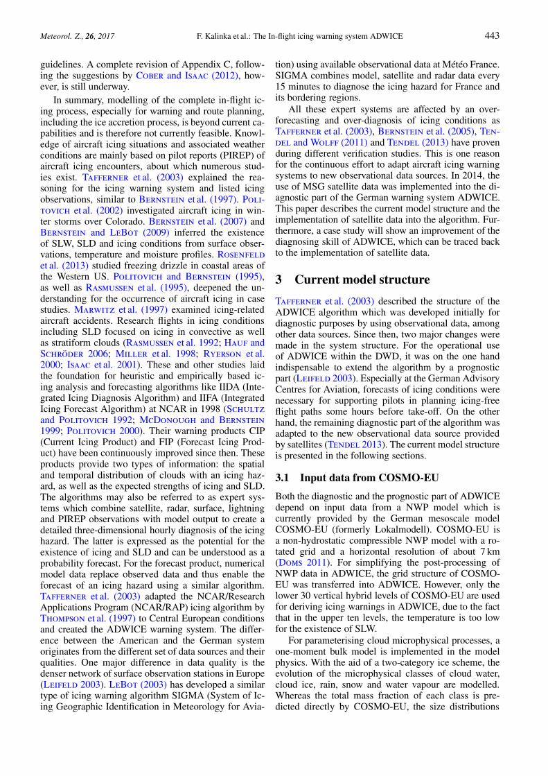
Figure 1: Algorithm structure of the German aircraft icing warningsystem ADWICE: the Prognostic Icing Product PIP is generated byrunning the PIA-algorithm with COSMO-EU data as input data.The combination of PIP, observations and model data in the DIA-algorithm results in the Diagnostic Icing Product DIP.

of the particles are assumed to be monodisperse for thenon-precipitating classes, and exponentially distributedwith respect to the hydrometeor diameter for the precip-itating classes (Doms et al. 2011). Furthermore, neitherthe transport nor the chemical composition of ice nucleiare implemented in the parameterisation of cloud mi-crophysical processes; just a temperature dependent icenuclei concentration is included. Therefore, a satisfac-tory description of the inhomogeneous freezing processas well as the amount and spatial distribution of liquidwater content cannot be supplied currently by COSMO-EU (Roloff 2012; Köhler and Görsdorf 2014).

3.2 Algorithm to forecast icing conditions

The Prognostic Icing Algorithm PIA receives COSMO-EU input data as illustrated in Figure 1. The fore-cast profiles of temperature and specific humidity arescanned by PIA to distinguish between four differenticing scenarios resulting in the Prognostic Icing Prod-uct (PIP), as will be explained in the following sub-sections. The thresholds for temperature and humidityrequired by these scenarios were originally derived forthe IIDA algorithm and were based on observationaldata in the vicinity of icing PIREPs (Thompson et al.1997; Schultz and Politovich 1992). They later wereadapted to European conditions by Leifeld (2003). Theclassification into four icing scenarios reflects the ex-pected droplet sizes within the predicted icing areas, in-cluding SLD. After identifying the relevant specific sce-nario, the associated icing intensity is derived from me-teorological parameters. A detailed description of thiscalculation is given in Section 3.4.

3.2.1 Scenario “Freezing”

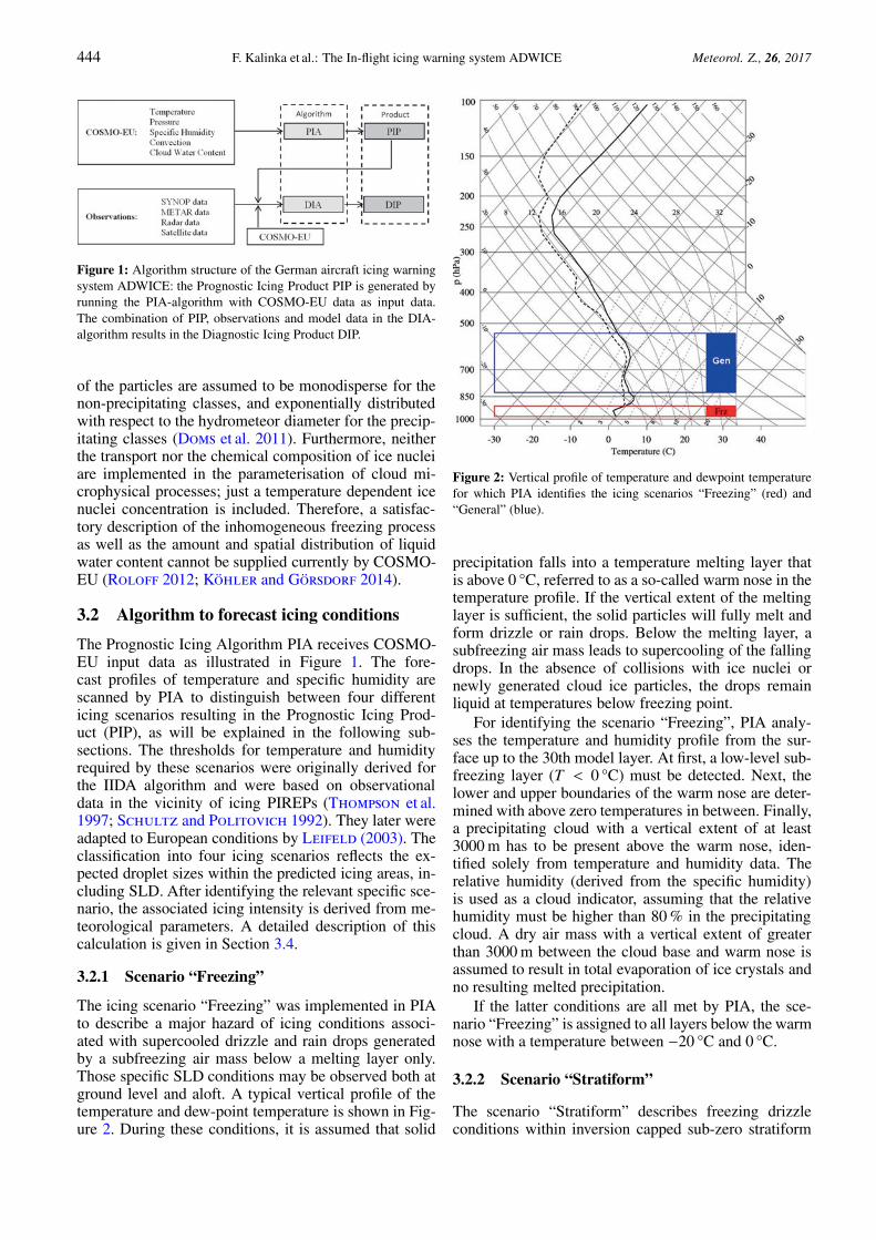
The icing scenario “Freezing” was implemented in PIAto describe a major hazard of icing conditions associ-ated with supercooled drizzle and rain drops generatedby a subfreezing air mass below a melting layer only.Those specific SLD conditions may be observed both atground level and aloft. A typical vertical profile of thetemperature and dew-point temperature is shown in Fig-ure 2. During these conditions, it is assumed that solid

Figure 2: Vertical profile of temperature and dewpoint temperaturefor which PIA identifies the icing scenarios “Freezing” (red) and“General” (blue).

precipitation falls into a temperature melting layer thatis above 0 °C, referred to as a so-called warm nose in thetemperature profile. If the vertical extent of the meltinglayer is sufficient, the solid particles will fully melt andform drizzle or rain drops. Below the melting layer, asubfreezing air mass leads to supercooling of the fallingdrops. In the absence of collisions with ice nuclei ornewly generated cloud ice particles, the drops remainliquid at temperatures below freezing point.

For identifying the scenario “Freezing”, PIA analy-ses the temperature and humidity profile from the sur-face up to the 30th model layer. At first, a low-level sub-freezing layer (T < 0 °C) must be detected. Next, thelower and upper boundaries of the warm nose are deter-mined with above zero temperatures in between. Finally,a precipitating cloud with a vertical extent of at least3000 m has to be present above the warm nose, iden-tified solely from temperature and humidity data. Therelative humidity (derived from the specific humidity)is used as a cloud indicator, assuming that the relativehumidity must be higher than 80 % in the precipitatingcloud. A dry air mass with a vertical extent of greaterthan 3000 m between the cloud base and warm nose isassumed to result in total evaporation of ice crystals andno resulting melted precipitation.

If the latter conditions are all met by PIA, the sce-nario “Freezing” is assigned to all layers below the warmnose with a temperature between −20 °C and 0 °C.

3.2.2 Scenario “Stratiform”

The scenario “Stratiform” describes freezing drizzleconditions within inversion capped sub-zero stratiform

Meteorol. Z., 26, 2017 F. Kalinka et al.: The In-flight icing warning system ADWICE 445

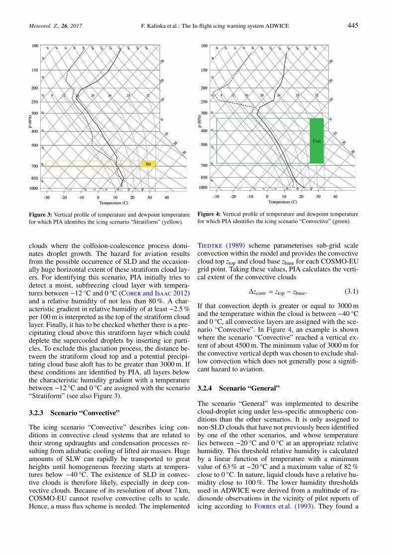
Figure 3: Vertical profile of temperature and dewpoint temperaturefor which PIA identifies the icing scenario “Stratiform” (yellow).

clouds where the collision-coalescence process domi-nates droplet growth. The hazard for aviation resultsfrom the possible occurrence of SLD and the occasion-ally huge horizontal extent of these stratiform cloud lay-ers. For identifying this scenario, PIA initially tries todetect a moist, subfreezing cloud layer with tempera-tures between −12 °C and 0 °C (Cober and Isaac 2012)and a relative humidity of not less than 80 %. A char-acteristic gradient in relative humidity of at least −2.5 %per 100 m is interpreted as the top of the stratiform cloudlayer. Finally, it has to be checked whether there is a pre-cipitating cloud above this stratiform layer which coulddeplete the supercooled droplets by inserting ice parti-cles. To exclude this glaciation process, the distance be-tween the stratiform cloud top and a potential precipi-tating cloud base aloft has to be greater than 3000 m. Ifthese conditions are identified by PIA, all layers belowthe characteristic humidity gradient with a temperaturebetween −12 °C and 0 °C are assigned with the scenario“Stratiform” (see also Figure 3).

3.2.3 Scenario “Convective”

The icing scenario “Convective” describes icing con-ditions in convective cloud systems that are related totheir strong updraughts and condensation processes re-sulting from adiabatic cooling of lifted air masses. Hugeamounts of SLW can rapidly be transported to greatheights until homogeneous freezing starts at tempera-tures below −40 °C. The existence of SLD in convec-tive clouds is therefore likely, especially in deep con-vective clouds. Because of its resolution of about 7 km,COSMO-EU cannot resolve convective cells to scale.Hence, a mass flux scheme is needed. The implemented

Figure 4: Vertical profile of temperature and dewpoint temperaturefor which PIA identifies the icing scenario “Convective” (green).

Tiedtke (1989) scheme parameterises sub-grid scaleconvection within the model and provides the convectivecloud top ztop and cloud base zbase for each COSMO-EUgrid point. Taking these values, PIA calculates the verti-cal extent of the convective clouds

Δzconv = ztop − zbase. (3.1)

If that convection depth is greater or equal to 3000 mand the temperature within the cloud is between −40 °Cand 0 °C, all convective layers are assigned with the sce-nario “Convective”. In Figure 4, an example is shownwhere the scenario “Convective” reached a vertical ex-tent of about 4500 m. The minimum value of 3000 m forthe convective vertical depth was chosen to exclude shal-low convection which does not generally pose a signifi-cant hazard to aviation.

3.2.4 Scenario “General”

The scenario “General” was implemented to describecloud-droplet icing under less-specific atmospheric con-ditions than the other scenarios. It is only assigned tonon-SLD clouds that have not previously been identifiedby one of the other scenarios, and whose temperaturelies between −20 °C and 0 °C at an appropriate relativehumidity. This threshold relative humidity is calculatedby a linear function of temperature with a minimumvalue of 63 % at −20 °C and a maximum value of 82 %close to 0 °C. In nature, liquid clouds have a relative hu-midity close to 100 %. The lower humidity thresholdsused in ADWICE were derived from a multitude of ra-diosonde observations in the vicinity of pilot reports oficing according to Forbes et al. (1993). They found a

446 F. Kalinka et al.: The In-flight icing warning system ADWICE Meteorol. Z., 26, 2017

mean relative humidity of 82 % with a standard devia-tion of 19 % (therefore the thresholds 63 % and 82 % inthe algorithm). The scenario “General” is also applied toupper layers in multilayer icing conditions above one ofthe previously defined icing scenarios. Figure 2 showssuch a multilayer situation with the scenario “Freezing”identified near the surface and the scenario “General”aloft. The precipitating cloud which is needed for theidentification of the scenario “Freezing” is assigned withthe icing scenario “General” in this case.

3.3 Algorithm to diagnose icing conditions

Icing forecasts based solely on humidity and temper-ature thresholds from model data (like in PIA) gener-ally produce a high false alarm rate (Tafferner et al.2003). This mainly is a result of the model’s grid reso-lution, which is too coarse to resolve clouds correctly.Lower thresholds of relative humidity result in higherrates of false alarms (because of the overestimation oficing). Using a high threshold of relative humidity as-sumes that we rely on a numerical model to forecastclouds correctly. Therefore, the aim is to use thresholdsthat will lead to a high probability of detection and alow false alarm rate. Thompson et al. (1997) did notsucceed in tuning relative humidity, and therefore sug-gested to use icing predictions as a first guess and im-prove it by using additional data from satellites, synop-tical stations (SYNOP) or RADAR. In the DiagnosticIcing Algorithm (DIA) of ADWICE, the model-basedPIP described in Section 3.2 is therefore initially used asa first guess of icing conditions. To minimise a possiblyhigh false alarm rate, assigned icing scenarios of PIP areconfirmed, extended or rejected by surface observationsfrom SYNOP stations, METeorological Aerodrome Re-ports (METAR) and by remote sensing data from radarinformation. Nevertheless, there exists a lack of opera-tionally available, widely distributed and systematic sur-face observations of vertical information about cloudceiling, the temperature and the humidity profile. How-ever, this information is necessary to find a possiblemelting layer as well as the vertical extent of a possibleicing risk. Using additional remote sensing data sourcesthat have become operational in recent years, the falsealarm rate can be further reduced in many situations.Such satellite derived products are used in a further stepfor identifying (non) hazardous clouds and for determin-ing their vertical extent. In the current Diagnostic IcingAlgorithm (DIA), operated by DWD, surface observa-tions are still treated as the most direct and reliable datasources, followed by remote sensing retrievals (radar,satellite data), followed by model data.

Tafferner et al. (2003) explicitly described the im-plementation of observation and radar data into DIA.Therefore, the following chapter will mainly focus ona detailed explanation of the integration of satellite dataand only briefly describe the fusion of synoptic and radardata.

3.3.1 Synoptic data

According to Bernstein and LeBot (2009), there is astrong correlation between defined surface weather phe-nomena and the detection of supercooled droplets inclouds and precipitation. Cloud ceiling and cloud type aswell as significant weather are reported by ground obser-vations and provide a first guess, not only about the lo-cation of clouds, but also about their vertical dimensionand the cloud phase. In accordance with the previouslydescribed four icing scenarios (“Stratiform”, “Convec-tive”, “Freezing” and “General”), DIA tries to identifypossible icing scenarios by using observed weather in-formation from SYNOP and METAR reports. Showerand thunderstorms, for example, indicate a strong ver-tical development of clouds and, therefore, a likely ex-istence of supercooled liquid droplets (scenario “Con-vective” confirmed). Drizzle is typically an indicator fora thin cloud layer and, therefore, possibly confirms thestratiform icing risk. Snowfall is a sign that icing condi-tions are likely non-existent as supercooled water doesnot persist in the presence of ice crystals because ofriming and/or the Bergeron-Findeisen process (Prup-pacher and Klett 1997) (icing scenarios rejected). Iffreezing rain is observed at the surface, it is a directproof of the existence of supercooled large droplets aloftbetween the ground and the melting layer and, therefore,the icing scenario “Freezing” is set or confirmed. Be-cause weather reports by automatic stations still sufferfrom quality deficiencies, especially for freezing precip-itation, only information from manned stations are cur-rently used in DIA.

Weather observations are normally valid for the ge-ographical location they are made, e.g., the precipita-tion amount. On the other hand, cloud observations re-fer to a larger area. In practice, the observed weatherphenomenon is interpreted as a representative informa-tion source for a certain surrounding area. To definethe validity area around an observation, the “Voronoi-Method” is applied (DeBerg et al. 2000) which subdi-vides the model domain into a honeycomb of polygonalcells, each with a weather station at its centre. The cellborders are drawn at the halfway point to neighbouringweather stations or at 70 km, whichever is closer. Everygrid point of the model domain located in one such cellis associated with the observation value of the respectiveweather station. Further information about transferringspatial fixed weather observations to the ADWICE gridare found in Leifeld (2003).

3.3.2 European radar composite

A radar reflectivity product from a Europe-wide weatherradar network is used to detect possible icing risk ar-eas. A reflectivity higher than 19 dBZ suggests a weathersituation with rain or snowfall while values lower than19 dBZ are typical for uniform stratiform clouds withechoes caused by drizzle, small rain droplets, or smallsnowflakes (scenario “Stratiform” confirmed). Radardata thus are helpful in identifying some current weathersituations, including clouds with icing risk.

Meteorol. Z., 26, 2017 F. Kalinka et al.: The In-flight icing warning system ADWICE 447

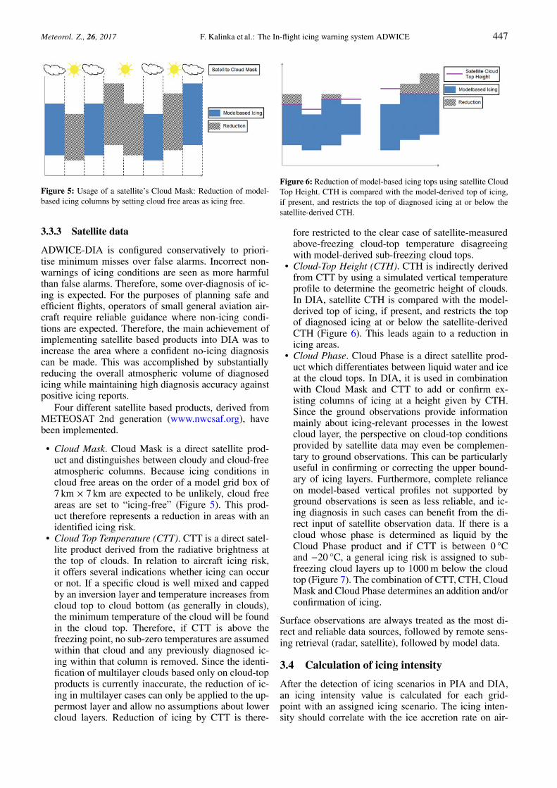
Figure 5: Usage of a satellite’s Cloud Mask: Reduction of model-based icing columns by setting cloud free areas as icing free.

3.3.3 Satellite data

ADWICE-DIA is configured conservatively to priori-tise minimum misses over false alarms. Incorrect non-warnings of icing conditions are seen as more harmfulthan false alarms. Therefore, some over-diagnosis of ic-ing is expected. For the purposes of planning safe andefficient flights, operators of small general aviation air-craft require reliable guidance where non-icing condi-tions are expected. Therefore, the main achievement ofimplementing satellite based products into DIA was toincrease the area where a confident no-icing diagnosiscan be made. This was accomplished by substantiallyreducing the overall atmospheric volume of diagnosedicing while maintaining high diagnosis accuracy againstpositive icing reports.

Four different satellite based products, derived fromMETEOSAT 2nd generation (www.nwcsaf.org), havebeen implemented.

• Cloud Mask. Cloud Mask is a direct satellite prod-uct and distinguishes between cloudy and cloud-freeatmospheric columns. Because icing conditions incloud free areas on the order of a model grid box of7 km × 7 km are expected to be unlikely, cloud freeareas are set to “icing-free” (Figure 5). This prod-uct therefore represents a reduction in areas with anidentified icing risk.

• Cloud Top Temperature (CTT). CTT is a direct satel-lite product derived from the radiative brightness atthe top of clouds. In relation to aircraft icing risk,it offers several indications whether icing can occuror not. If a specific cloud is well mixed and cappedby an inversion layer and temperature increases fromcloud top to cloud bottom (as generally in clouds),the minimum temperature of the cloud will be foundin the cloud top. Therefore, if CTT is above thefreezing point, no sub-zero temperatures are assumedwithin that cloud and any previously diagnosed ic-ing within that column is removed. Since the identi-fication of multilayer clouds based only on cloud-topproducts is currently inaccurate, the reduction of ic-ing in multilayer cases can only be applied to the up-permost layer and allow no assumptions about lowercloud layers. Reduction of icing by CTT is there-

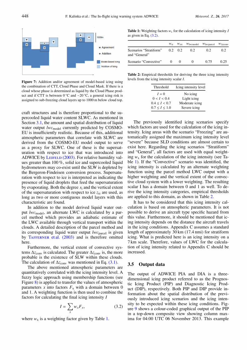
Figure 6: Reduction of model-based icing tops using satellite CloudTop Height. CTH is compared with the model-derived top of icing,if present, and restricts the top of diagnosed icing at or below thesatellite-derived CTH.

fore restricted to the clear case of satellite-measuredabove-freezing cloud-top temperature disagreeingwith model-derived sub-freezing cloud tops.

• Cloud-Top Height (CTH). CTH is indirectly derivedfrom CTT by using a simulated vertical temperatureprofile to determine the geometric height of clouds.In DIA, satellite CTH is compared with the model-derived top of icing, if present, and restricts the topof diagnosed icing at or below the satellite-derivedCTH (Figure 6). This leads again to a reduction inicing areas.

• Cloud Phase. Cloud Phase is a direct satellite prod-uct which differentiates between liquid water and iceat the cloud tops. In DIA, it is used in combinationwith Cloud Mask and CTT to add or confirm ex-isting columns of icing at a height given by CTH.Since the ground observations provide informationmainly about icing-relevant processes in the lowestcloud layer, the perspective on cloud-top conditionsprovided by satellite data may even be complemen-tary to ground observations. This can be particularlyuseful in confirming or correcting the upper bound-ary of icing layers. Furthermore, complete relianceon model-based vertical profiles not supported byground observations is seen as less reliable, and ic-ing diagnosis in such cases can benefit from the di-rect input of satellite observation data. If there is acloud whose phase is determined as liquid by theCloud Phase product and if CTT is between 0 °Cand −20 °C, a general icing risk is assigned to sub-freezing cloud layers up to 1000 m below the cloudtop (Figure 7). The combination of CTT, CTH, CloudMask and Cloud Phase determines an addition and/orconfirmation of icing.

Surface observations are always treated as the most di-rect and reliable data sources, followed by remote sens-ing retrieval (radar, satellite), followed by model data.

3.4 Calculation of icing intensity

After the detection of icing scenarios in PIA and DIA,an icing intensity value is calculated for each grid-point with an assigned icing scenario. The icing inten-sity should correlate with the ice accretion rate on air-

448 F. Kalinka et al.: The In-flight icing warning system ADWICE Meteorol. Z., 26, 2017

Figure 7: Addition and/or agreement of model-based icing usingthe combination of CTT, Cloud Phase and Cloud Mask. If there is acloud whose phase is determined as liquid by the Cloud Phase prod-uct and if CTT is between 0 °C and −20 °C, a general icing risk isassigned to sub-freezing cloud layers up to 1000 m below cloud top.

craft structures and is therefore proportional to the su-percooled liquid water content SLWC. As mentioned inSection 3.1, the amount and spatial distribution of liquidwater output lwcmodel currently predicted by COSMO-EU is insufficiently realistic. Because of this, additionalatmospheric parameters that correlate with SLWC arederived from the COSMO-EU model output to serveas a proxy for SLWC. One of these is the supersat-uration with respect to ice that was introduced intoADWICE by Leifeld (2003). For relative humidity val-ues greater than 100 %, solid ice and supercooled liquidhydrometeors may co-exist until the SLW is depleted bythe Bergeron-Findeisen conversion process. Supersatu-ration with respect to ice is interpreted as indicating thepresence of liquid droplets that feed the supersaturationby evaporating. Both the degree si and the vertical extentof the supersaturation with respect to ice zsi are used, aslong as two or more contiguous model layers with thischaracteristic are found.

In addition to the model derived liquid water out-put lwcmodel, an alternate LWC is calculated by a par-cel method which provides an adiabatic estimate ofthe LWC available through vertical transport within theclouds. A detailed description of the parcel method andits corresponding liquid water output lwcparcel is givenby Tafferner et al. (2003) and is therefore omittedhere.

Furthermore, the vertical extent of convective sys-tems Δzconv is calculated. The greater Δzconv is, the moreprobable is the existence of SLW within these clouds.The calculation of Δzconv was mentioned in Eq. (3.1).

The above mentioned atmospheric parameters arequantitatively correlated with the icing intensity level. Afuzzy logic approach using membership functions (seeFigure 8) is applied to transfer the values of atmosphericparameters x into factors Fx with a domain between 0and 1. A weighting function is then used to combine thefactors for calculating the final icing intensity I

I =∑

x

wxFx, (3.2)

where wx is a weighting factor given by Table 1.

Table 1: Weighting factors wx for the calculation of icing intensity Ias given in Eq. (3.2).

wsi wzsi wlwcmodel wlwcparcel wΔzconv

Scenarios “Stratiform”and “General”

0.2 0.2 0.2 0.2 0.2

Scenario “Convective” 0 0 0 0.75 0.25

Table 2: Empirical thresholds for deriving the three icing intensitylevels from the icing intensity scalar I.

Threshold Icing intensity level

I = 0 No icing0 < I < 0.4 Light icing

0.4 ≤ I < 0.7 Moderate icing0.7 ≤ I ≤ 1.0 Severe icing

The previously identified icing scenarios specifywhich factors are used for the calculation of the icing in-tensity. Icing areas with the scenario “Freezing” are au-tomatically assigned the maximum icing intensity level“severe” because SLD conditions are almost certain toexist here. Regarding the icing scenarios “Stratiform”and “General”, all factors are used with equal weight-ing wx for the calculation of the icing intensity (see Ta-ble 1). If the “Convective” scenario was identified, theicing intensity is calculated by an alternate weightingfunction using the parcel method LWC output with ahigher weighting and the vertical extent of the convec-tive cloud system with a lower weighting. The resultingscalar I has a domain between 0 and 1 as well. To de-rive the icing intensity categories, empirical thresholdsare applied to this domain, as shown in Table 2.

It has to be considered that this icing intensity cal-culation is based on atmospheric parameters. It is notpossible to derive an aircraft type specific hazard fromthis value. Furthermore, it should be mentioned that ic-ing intensity depends on the distance the aircraft travelsin the icing conditions. Appendix C assumes a standardlength of approximately 30 km (17.4 nmi) for stratiformicing. What is predicted here is an icing intensity on a7 km scale. Therefore, values of LWC for the calcula-tion of icing intensity related to Appendix C should beincreased.

3.5 Output data

The output of ADWICE PIA and DIA is a three-dimensional icing product referred to as the Prognos-tic Icing Product (PIP) and Diagnostic Icing Prod-uct (DIP), respectively. Both PIP and DIP provide in-formation about the spatial distribution of the previ-ously introduced icing scenarios and the icing inten-sity to be expected within these icing conditions. Fig-ure 9 shows a colour-coded graphical output of the PIPin a top-down composite view showing column max-ima for 04:00 UTC 06 November 2013. This example

Meteorol. Z., 26, 2017 F. Kalinka et al.: The In-flight icing warning system ADWICE 449

Figure 8: Membership functions Fx for the calculation of icing intensity as given in Eq. (3.2). S i is the degree, zsi the vertical extent ofsupersaturation with respect to ice, Δzconv the vertical extent of convective clouds (Eq. (3.1)), lwcmodel the liquid water content derived by themodel and lwcparcel the liquid water content derived by the parcel method.

Figure 9: Illustration of the ADWICE output PIP. Left: a composite view presenting the distribution of the four icing scenarios“General” (blue), “Convective” (green), “Stratiform” (yellow) and “Freezing” (red). Right: the associated icing intensity within the threeintensity levels “Light” (green), “Moderate” (yellow) and “Severe” (red).

case demonstrates that ADWICE is capable of resolvingalso small-scale icing conditions, e.g., within a clusterof thunderstorms to the northeast of Sicily which wereverified by a pilot reporting moderate icing conditions inthis area.

PIA runs operationally at DWD and is updated fourtimes a day at about 03, 09, 15 and 21 UTC follow-ing the main runs of COSMO-EU at 00, 06, 12 and18 UTC. PIA provides an hourly forecast 21 hours ahead(00/06/12/18 UTC + 4 h, + 5 h, . . . , 24 h), followed bya three-hourly forecast between the forecast times +24 hand +48 h, followed by a six-hourly forecast between theforecast times +48 h and +78 h. In contrast, DIA runs ev-ery hour based on the current PIP and all necessary ob-servational data. PIP and DIP are both available across30 model layers and interpolated to 12 flight levels.

4 Verification against pilot reports overEurope

A validation study was performed to quantify the impactof the above described implementation of satellite de-rived data in ADWICE-DIA. For this purpose, the prog-nostic and the diagnostic icing products (with and with-out implemented satellite data) are separately comparedwith pilot reports.

4.1 Validation data and quality

PIREPS currently represents the only widely availabledataset for direct in-situ icing observations aloft thatcan identify the existence of supercooled liquid water inthe atmosphere. However, over Europe there are someproblematic properties that must be considered:

450 F. Kalinka et al.: The In-flight icing warning system ADWICE Meteorol. Z., 26, 2017

• Pilot observed icing intensity is subjective and is de-fined by the impact on aircraft handling, which de-pends, e.g., on the size and speed of the aircraft, theangle of attack, the aircraft de-icing system on board,if any, and on other factors. Severe icing for a smallsports airplane without any de-icing system may beregarded as trace ice for bigger airplanes with heatedwings. The severity of reported icing is insufficientlydefined to compare directly with model-derived icingintensity. For this reason, all observed icing degreeslight, moderate and severe are summarised in the fol-lowing evaluation as a positive observation (“YES”).

• PIREPS are human-based. If a pilot notices ice ac-cumulation, countermeasures (activation of de-icing,descending or climbing, etc.) have to be initiatedfirst. In general, the report is transmitted as soon asthe aircraft is in a less stressful situation for the pilot,thus allowing him to report the event to the ground.Altogether, this results in time delays and an inaccu-rate horizontal and vertical location of the observedevent.

• The transmission of a PIREP is requested of pilotsbut is not obligatory, so that not all events are re-ported.

• “No icing” is rarely reported. However, negative ob-servations are essential for validation studies. To in-crease the dataset of “no icing events”, a PIREP re-porting “clear above” is handled as an implicit “noicing” report for the cloud-free area above.

• In summary, PIREPs exhibit strong category biastowards positive events and distribution bias aroundicing areas. On top of this, PIREPs are also naturallybiased in their distribution towards areas of high airtraffic density.

PIREPs over Europe are often signed by hand and af-terwards not transmitted to the meteorological offices.There is no centralised and unified European collectionsystem so that data are easily lost or even not trans-mitted because of time constraints, depending on theweather situation. Nevertheless, the PIREP data is cur-rently the only source to verify forecasting systems forin-flight icing. The validation study presented here re-quired the comparison of point observations (PIREPs)with point forecast/diagnosis values derived from thegridded ADWICE output. In order to consider inaccu-racies in space and time in the observations as well as inthe model output, the required point value for the fore-cast/diagnosis was not simply taken from the grid pointclosest to the observation, but rather generated from sev-eral grid points around the observation. The maximumof predicted and diagnosed icing in a generated cube of7× 7 horizontal and three vertical model grid boxes (ap-proximately 49 × 49 km in horizontal; vertical distancedepends on the level and surface height: the closer tothe surface, the lower the distance in between the lev-els, and vice versa) was compared with the PIREP infor-mation. For time consideration, always the next forecasthour to the observational time according to Section 3.5

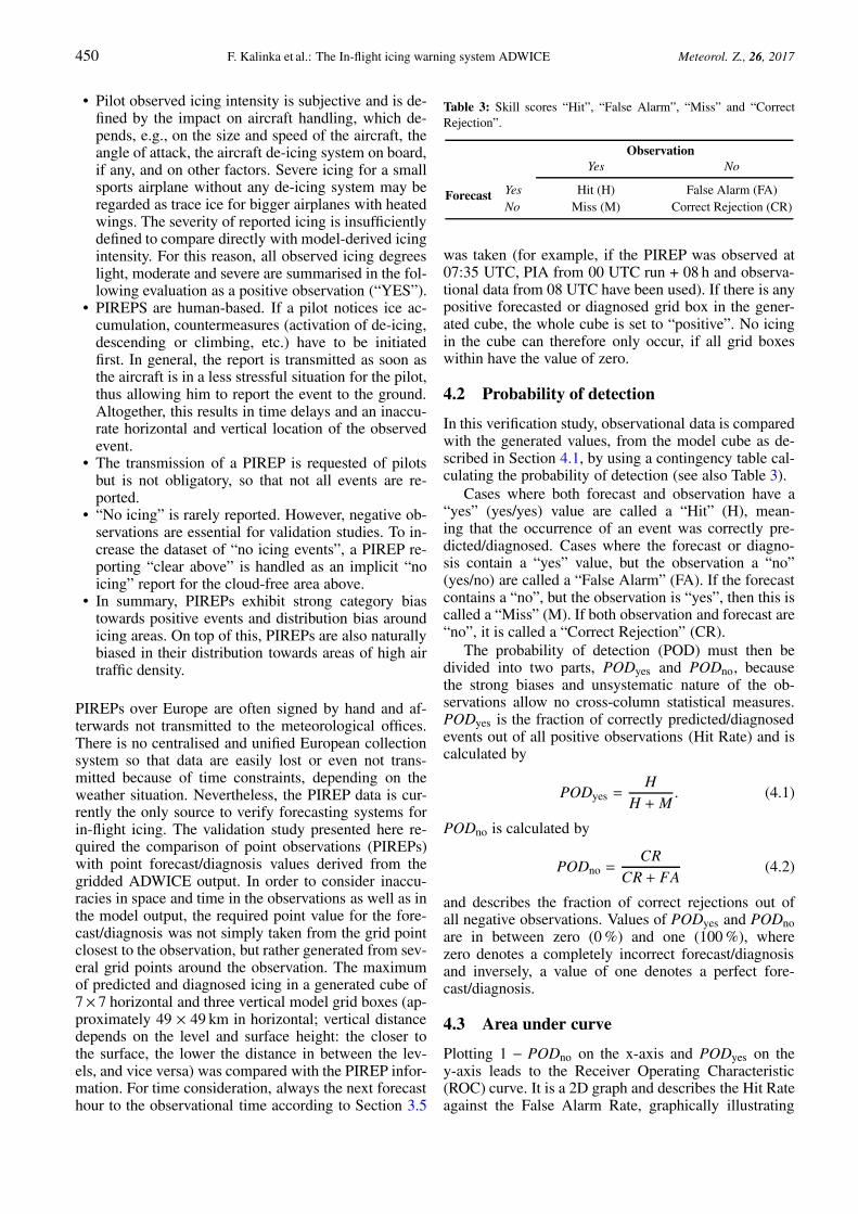
Table 3: Skill scores “Hit”, “False Alarm”, “Miss” and “CorrectRejection”.

ObservationYes No

Forecast Yes Hit (H) False Alarm (FA)No Miss (M) Correct Rejection (CR)

was taken (for example, if the PIREP was observed at07:35 UTC, PIA from 00 UTC run + 08 h and observa-tional data from 08 UTC have been used). If there is anypositive forecasted or diagnosed grid box in the gener-ated cube, the whole cube is set to “positive”. No icingin the cube can therefore only occur, if all grid boxeswithin have the value of zero.

4.2 Probability of detection

In this verification study, observational data is comparedwith the generated values, from the model cube as de-scribed in Section 4.1, by using a contingency table cal-culating the probability of detection (see also Table 3).

Cases where both forecast and observation have a“yes” (yes/yes) value are called a “Hit” (H), mean-ing that the occurrence of an event was correctly pre-dicted/diagnosed. Cases where the forecast or diagno-sis contain a “yes” value, but the observation a “no”(yes/no) are called a “False Alarm” (FA). If the forecastcontains a “no”, but the observation is “yes”, then this iscalled a “Miss” (M). If both observation and forecast are“no”, it is called a “Correct Rejection” (CR).

The probability of detection (POD) must then bedivided into two parts, PODyes and PODno, becausethe strong biases and unsystematic nature of the ob-servations allow no cross-column statistical measures.PODyes is the fraction of correctly predicted/diagnosedevents out of all positive observations (Hit Rate) and iscalculated by

PODyes =H

H + M. (4.1)

PODno is calculated by

PODno =CR

CR + FA(4.2)

and describes the fraction of correct rejections out ofall negative observations. Values of PODyes and PODnoare in between zero (0 %) and one (100 %), wherezero denotes a completely incorrect forecast/diagnosisand inversely, a value of one denotes a perfect fore-cast/diagnosis.

4.3 Area under curve

Plotting 1 − PODno on the x-axis and PODyes on they-axis leads to the Receiver Operating Characteristic(ROC) curve. It is a 2D graph and describes the Hit Rateagainst the False Alarm Rate, graphically illustrating

Meteorol. Z., 26, 2017 F. Kalinka et al.: The In-flight icing warning system ADWICE 451

additional characteristics of forecast/diagnosis skill. Thecurve is plotted beginning in x = 0 and y = 0, throughall POD pairs and ends in x = 1 and y = 1. The areain between the x-axis and the ROC-curve is called the“Area Under Curve” (AUC), representing a measure ofthe forecast’s ability to discriminate between “yes” and“no” observations. An AUC value of 0.5 represents arandom equivalent forecast, values above 0.5 representa better forecast, values below 0.5 a worse forecast.

4.4 Volume efficiency

PIREPS are usually reported to warn following aircraftin case of any severe weather event. Accordingly, non-severe weather reports are nearly unimportant for flightsafety so that they are reported rarely. This low numberof data points makes it difficult to determine a reliabletrue False Alarm Rate for the diagnosis and forecasts ofADWICE. The concept of volume efficiency is thereforeused as an alternative, since it can help illustrate the rel-ative amount of spatial-volume different-diagnosis out-puts assigned with the icing potential to achieve theirhit rate. This relationship between PODyes and the ic-ing volume simulated in a prognosis or diagnosis is de-scribed by

Voleff = 100 ·PODyes

Vol%, (4.3)

where the icing volume percentage is defined as

Vol% = 100 ·Volice

Voltot. (4.4)

Here, Volice is the summed volume of all grid points withan associated positive event and Voltot is the summedvolume of all grid points. The Volume Efficiency setsthe values of PODyes in relation to the fraction of totalpredicted/diagnosed icing. The higher Voleff, the morereliable PODyes. This approach is therefore very usefulin simulations where a reliable PODyes may be calcu-lated from a large number of positive observations, but alow number of negative observations leads to an unreli-able PODno. It must be stressed, however, that absolutevalues for Vol% and Voleff are in themselves meaning-less and are only useful to illustrate differences in al-gorithm configurations that run on otherwise identicalmodel grids (constant Voltot).

4.5 Results

From October 2013 to the end of January 2014, 848PIREPS with positive and negative icing informationwere collected over Europe. The geographic distributionis shown in Figure 10. In 824 cases, at least “light ic-ing” was observed, where in only 24 cases, “no icing”or “clear above” were reported. Neglecting the reportedicing intensity, every PIREP was compared with its as-sociated “model cube” as described in Section 4.1. Thecalculated skill scores can be found in Table 4.

Figure 10: Location of 848 observed PIREPS over Europe betweenOctober 2013 and January 2014. Green = light, yellow = moderate,red = severe and blue = no icing observed.

Table 4: Results of PIA and DIA with and without satellite data incomparison with pilot icing observations.

PODyes (%) PODno (%) Vol% Voleff AUC

Prognosis 90.78 62.5 12.7 7.14 0.77

Diagnosis,without sat.-data

88.11 62.5 11.4 7.72 0.75

Diagnosis,with sat.-data

88.47 62.5 9.54 9.28 0.75

With nearly 91 %, PIP shows the best results in HitRate, whereas DIP, both with and without satellite data,has a slightly lower Hit Rate of ca. 88 %. PODno staysequal in all three runs at 62.5 % due to the low num-ber of 24 “no icing” observations. The correspondingAUC values are 0.77 for PIA and 0.75 for both DIAversions. Initially, it is notable that the Hit Rate doesnot increase for DIA, even though observational data isused. But filling all model grid points with a positiveicing event would lead to a Hit Rate of 100 % as wellas to a False Alarm Rate of 100 %. This is the reasonwhy a few negative observations cannot be a reliable ba-sis for finding a significant statistical conclusion aboutPODno and about the model performance. Due to thelack of negative observations, the Volume Efficiency de-scribed in Section 4.4 was introduced to allow a conclu-sion about model performance: the higher the Volumeefficiency, the better the model performance. Results forVolume Efficiency were raised from 7.14 in PIA to 7.72in DIA without satellite data, and finally to 9.28 in DIAusing satellite data. Fewer grid points are assigned icingconditions while the hit rate remains high.

The influence of the individual satellite products aswell as of SYNOP and RADAR data on icing diagnosis

452 F. Kalinka et al.: The In-flight icing warning system ADWICE Meteorol. Z., 26, 2017

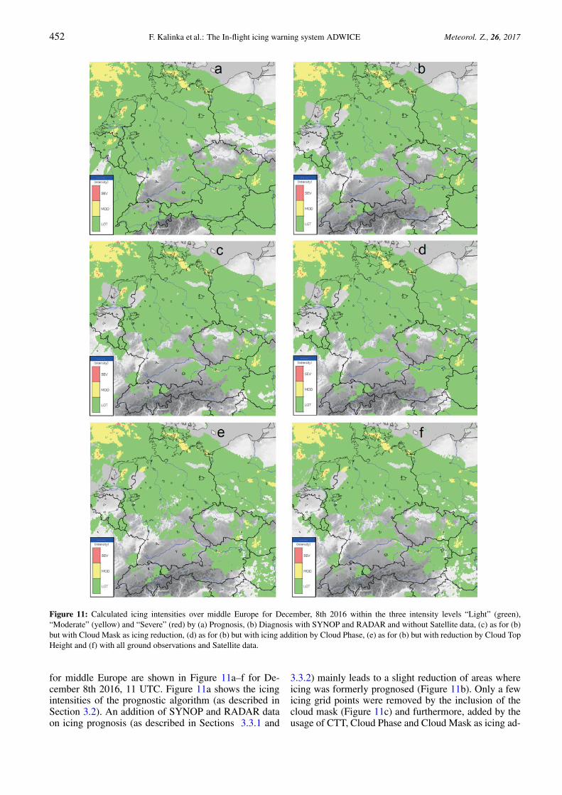
Figure 11: Calculated icing intensities over middle Europe for December, 8th 2016 within the three intensity levels “Light” (green),“Moderate” (yellow) and “Severe” (red) by (a) Prognosis, (b) Diagnosis with SYNOP and RADAR and without Satellite data, (c) as for (b)but with Cloud Mask as icing reduction, (d) as for (b) but with icing addition by Cloud Phase, (e) as for (b) but with reduction by Cloud TopHeight and (f) with all ground observations and Satellite data.

for middle Europe are shown in Figure 11a–f for De-cember 8th 2016, 11 UTC. Figure 11a shows the icingintensities of the prognostic algorithm (as described inSection 3.2). An addition of SYNOP and RADAR dataon icing prognosis (as described in Sections 3.3.1 and

3.3.2) mainly leads to a slight reduction of areas whereicing was formerly prognosed (Figure 11b). Only a fewicing grid points were removed by the inclusion of thecloud mask (Figure 11c) and furthermore, added by theusage of CTT, Cloud Phase and Cloud Mask as icing ad-

Meteorol. Z., 26, 2017 F. Kalinka et al.: The In-flight icing warning system ADWICE 453

ditions (see Figure 11d). The highest influence of satel-lite products has the usage of CTH for icing reductionof model-based icing tops (see Figure 11e). The final re-sult using all ground observations, RADAR and satellitedata is shown in Figure 11f.

In conclusion, the newly introduced satellite algo-rithm in DIA efficiently reduces over-forecasting rel-ative to PIA. Because of the low number of PIREPSover Europe, an additional validation campaign was per-formed over the United States, where a reliable numberof diverse pilot reports exist. Results for PODyes witha value of nearly 90 % are almost similar to those overEurope, whereas PODno (21.5 %) and AUC (0.556) aresomewhat lower than over Europe (Tendel 2013). Butagain, the satellite-based icing product of ADWICE wasable to reduce the overall icing volume percentage bybetween 10 % and 30 %. Furthermore, ADWICE wascompared with FIP in Tendel and Wolff (2011). Thestudy found good agreement in fundamental model skillindicated by stable and very similar AUC scores.

5 Conclusions and future work

ADWICE consists of a diagnostic part DIA, which maybe seen as a nowcasting system, and a very similarprognostic part PIA where the required observationalinput data are replaced by or estimated from modeloutput data. The icing diagnosis quality depends onthe amount, quality and type of input data. Standardinput data includes temperature and specific humidityfrom a NWP model, as well as SYNOP and METARinformation, radar, and satellite data.

In this paper, it was shown how the newly intro-duced satellite data are implemented in ADWICE andhow the overall quality of ADWICE was improved. Themain improvement in the use of satellite data broughtto ADWICE lies in the reduction of over-diagnosis byallowing the identification of additional icing-free areasin the model domain that were conservatively labelledas potential icing by the baseline algorithm. This reduc-tion in icing volume while maintaining a high rate ofcorrectly capturing reported icing encounters implies amore accurate placement of icing areas. This also in-creases trust in the diagnosis of no-icing conditions,an important factor for visual flight rules (VFR) flightsafety.

The various icing expert systems such as ADWICE,SIGMA (Meteo France) and CIP/FIP (NCAR) are ad-justed to the region to which they are applied. Oppor-tunities for optimisation lie in the differences in spatialavailability, e.g., for SYNOP data in Europe and in theUS and in the weighting with which those data enter thealgorithms.

Validation of ADWICE and other icing expert sys-tems is conventionally performed against PIREPs. Thesehave some significant deficiencies as validation data, butare, so far, the only readily available independent icinginformation source. Any warning scheme suffers from

significant over-forecasting, and correspondingly highfalse-alarm-rates. To quantify this, negative (no) icinginformation is needed, which unfortunately is not pro-vided in sufficient quality by PIREPs. This will hope-fully change in the future when aircraft data from ic-ing detectors will be included in the AMDAR data-link scheme and will be reported to the ground. PIREPsmostly report positive (“yes”) icing information. Icingdetector signals will consistently report “no icing” aswell. Experience shows that in more than 90 % of allcases, icing conditions are not present in a particularcloud. Systematic icing detector readings will alleviatethe category bias and the icing-related location bias ofPIREPs and report realistic fractions of icing vs. no-icing conditions along the flight path. The location biastoward areas with a high air-traffic density will remain,however. In the future, PIREPs may continue to be usedfor validation, as presented in this paper. However, theymay also be used as an additional information source innowcasting systems.

The AMDAR programme will also introduce air-borne humidity measurements in the near future. Fromthat data, one may infer the existence of clouds and icesupersaturation. Both measurement quantities would behugely beneficial in ADWICE and of course in all NWPmodels.

Besides the AMDAR measurements, other valuabledata sources will become operationally available in thefuture. One of them will be Doppler polarisation radarinformation and the coupled particle identification algo-rithm. This will allow, for instance, the direct detectionof liquid water vs. ice crystals in precipitation, enablingthe remote identification of supercooled freezing rain orinversely, the SLWC depletion potential of ice crystals.

In conclusion, the current ADWICE version hasproven to be a successful update to the system for diag-nosing supercooled liquid water content. There is, how-ever, still significant room for improvement concerningthe detection of SLWC and also of the icing severity.Future data sources, including the improved use of next-generation NWP output will serve to also improve theforecast products.

Acknowledgments

This work was funded by the DWD’s Research ProgramSFP 1.10.

References

Abbat,t J.P.D., S. Benz, D.J. Cziczo, Z.A. Kanji,U. Lohmann, O. Möhler, 2006: Solid AmmoniumSulfate Aerosols as Ice Nuclei: A Pathway for Cirrus CloudFormation. – Science 313, 1770–1773. DOI: 10.1126/science.1129726.

Andreae, M.O., D. Rosenfeld, 2008: Aerosol-cloud-precipitation interactions, Part 1: The nature and sourcesof cloud-active aerosols. – Earth-Sci. Rev. 89, 13–41. DOI:10.1016/j.earscirev.2008.03.001.

454 F. Kalinka et al.: The In-flight icing warning system ADWICE Meteorol. Z., 26, 2017

Appiah-Kubi P., 2011: U.S Inflight Icing Accidents and Inci-dents, 2006 to 2010. – Master thesis. University of Tennessee,Knoxville.

Bernstein, B.C., C. LeBot, 2009: An Inferred Climatology ofIcing Conditions Aloft, Including Supercooled Large Drops.Part II: Europe, Asia, and the Globe. – J. Appl. Meteor. Cli-matol. 48, 1503–1526. DOI: 10.1175/2009JAMC2073.1.

Bernstein, B.C., T.A. Omeron, F. McDonough,M.K. Politovich, 1997: The Relationship betweenAircraft Icing and Synoptic-Scale Weather Condi-tions. – Wea. Forecast. 12, 742–762. DOI: 10.1175/1520-0434(1997)012<0742:TRBAIA>2.0.CO;2.

Bernstein, B.C., F. McDonough, M.K. Politovich,B.G. Brown, 2005: Current Icing Potential: AlgorithmDescription and Comparison with Aircraft Observations. –J. Appl. Meteor. 44, 969–986. DOI: 10.1175/JAM2246.1.

Bernstein, B.C., C.A. Wolff, F. McDonough, 2007: An In-ferred Climatology of Icing Conditions Aloft, Including Su-percooled Large Drops. Part I: Canada and the ContinentalUnited States. – J. Appl. Meteor. Climatol. 46, 1857–1878.DOI: 10.1175/2007JAMC1607.1.

Christner, B.C., C.E. Morris, C.M. Foreman, R. Cai,D.C. Sands, 2008: Ubiquity of Biological Ice Nucle-ators in Snowfall. – Science 319, 1214. DOI: 10.1126/science.1149757.

Cober, S.G., G.A. Isaac, 2012: Characterization of Aircraft Ic-ing Environments with Supercooled Large Drops for Applica-tion to Commercial Aircraft Certification. – J. Appl. Meteor.Climatol. 51, 265–284. DOI: 10.1175/JAMC-D-11-022.1.

DeBerg, M., M. vanKreveld, M. Overmars, O. Schwarz-kopf, 2000: Voronoi Diagrams. – Computational Geometry:Algorithms and Applications, Springer 7, 147–163.

DeMott, P.J., D.J. Cziczo, A.J. Prenni, D.M. Murphy,S.M. Kreidenweis, D.S. Thomson, R. Borys, D.C. Rogers,2003: Measurements of the concentration and compositionof nuclei for cirrus formation. – Proceedings of the NationalAcademy of Sciences of the United States of America 100,14655–14660.

DeMott, P.J. and Coauthors, 2011: Resurgence in Ice Nu-clei Measurement Research. – Bull. Amer. Meteor. Soc. 92,1623–1635. DOI: 10.1175/2011BAMS3119.1.

Doms, G., 2011: A Description of the Nonhydrostatic RegionalCOSMO – Model. Part I: Dynamics and Numerics. – Tech-nical Report, Deutscher Wetterdienst, Offenbach, Germany,153 pp.

Doms, G., J. Förstner, E. Heise, H-J. Herzog, D. Mironov,M. Raschendorfer, T. Reinhardt, B. Ritter, R. Schro-din, J-P. Schulz, G. Vogel, 2011: A Description of theNonhydrostatic Regional COSMO – Model. Part II: PhysicalParameterizations. – Technical Report, Deutscher Wetterdi-enst, Offenbach, Germany, 161 pp.

Flossmann, A.I., W. Wobrock, 2010: A review of our under-standing of the aerosol cloud interaction from the perspec-tive of a bin resolved cloud scale modelling. – J. Atmos. Res.97(4), 478–497. DOI: 10.1016/j.atmosres.2010.05.008.

Forbes, G.S., Y. Hu, B.G. Brown, B.C.. Bernstein,M.K. Politovic, 1993: Examination of conditions in theproximity of pilot reports of icing during STORM-FEST. –Fifth International Conference on Aviation Weather Systems.2–6 August 1993, Vienna, Virginia, American MeteorologicalSociety, 282-286.

Green S.D., 2006: A study of U.S. Inflight Icing Accidents,1978 to 2002. – Proceedings of the 44th AIAA AerospaceSciences Meeting and Exhibit, AIAA 2006-82, Reno, Nevada.

Hauf, T., F. Schröder, 2006: Aircraft icing research flightsin embedded convection. – Meteorology and AtmosphericPhysics 91, 247–265. DOI: 10.1007/s00703-004-0082-y.

Hedde, T., D. Guffond, 1995: ONERA Three-DimensionalIcing Model. – AIAA Journal 33, 1038–1045.

Hung, H.M., A. Malinowski, S.T. Martin, 2003: Kinetics ofHeterogeneous Ice Nucleation on the Surfaces of Mineral DustCores Inserted into Aqueous Ammonium Sulfate Particles. –J. Phys. Chem. A 107, 1296–1306. DOI: 10.1021/jp021593y.

Isaac, G.A., S.J. Cober, J.W. Strapp, A.V. Korolev, A. Trem-blay, D.L. Marcotte, 2001: Recent Canadian research onaircraft in-flight icing. – Canadian Aeronautics Space J. 47,213–221.

Jeck, R.K., 2002: Icing Design Envelopes (14 CFR Parts 25and 29, Appendix C) Converted to a Distance-Based Format.DOT/FAA/AR-00/30. Federal Aviation Administration, Air-port and Aircraft Safety Research and Development, WilliamJ. Hughes Technical Center, Atlantic City International Air-port, NJ 08405. Final Report, available to the U.S. publicthrough the National Technical Information Service (NTIS),Springfield, Virginia 22161a.

Kärcher, B., O. Möhler, P.J.. DeMott, S. Pechtl, F. Yu,2007: Insights into the role of soot aerosols in cirrus cloudformation. – J. Atmos. Chem. Phys. 7, 4203–4227. DOI:10.5194/acp-7-4203-2007.

Köhler, F., U. Görsdorf, 2014: Towards 3D prediction ofsupercooled liquid water for aircraft icing: Modifications ofthe microphysics in COSMO-EU. – Meteorol. Z. 23, 253–262.DOI: 10.1127/metz/2014/0545.

Korolev, A.V., G.A. Isaac, S.G. Cober, J.W. Strapp, J. Hal-lett, 2003: Microphysical characterization of mixed-phaseclouds. – Quart. J. Roy. Meteor. Soc. 129, 39–65. DOI:10.1256/qj.01.204.

LeBot, C., 2003: SIGMA: System of Icing Geographic identi-fication in Meteorology for Aviation. – SAE Technical Paper.DOI: 10.4271/2003-01-2085.

Leifeld C., 2003: Weiterentwicklung des NowcastingsystemsADWICE zur Erkennung vereisungsgefährdeter Lufträume. –PhD thesis. Institute of Meteorology and Climatology, Gott-fried Wilhelm Leibniz Universität Hannover, Hannover, Ger-many, 113 pp.

Lohmann, U., K. Diehl, 2006: Sensitivity Studies of the Im-portance of Dust Ice Nuclei for the Indirect Aerosol Effect onStratiform Mixed-Phase Clouds. – J. Atmos. Sci. 63, 968–982.DOI: 10.1175/JAS3662.1.

Martin S.T., 1998: Phase transformations of the ternary sys-tem (NH4)2SO4-H2SO4-H2O and the implications for cirruscloud formation. – Geophys. Res. Lett. 25, 1657–1660.

Marwitz, J.D., M.K. Politovich, B.C. Bernstein,F.M. Ralph, P.J. Neiman, R. Ashenden, J. Bresch, 1997:Meteorological Conditions Associated with the ATR-72Aircraft Accident near Roselawn, Indiana on 31 October1994. – Bull. Amer. Meteor. Soc. 78, 41–52. DOI: 10.1175/1520-0477(1997)078<0041:MCAWTA>2.0.CO;2

McDonough, F., B.C. Bernstein, 1999: Combining satel-lite, radar and surface observations with model data to cre-ate a better aircraft icing diagnosis. – Proceedings of the8th Conference on Aviation, Range and Aerospace Meteorol-ogy. 10–15 January 1999, Dallas, TX, 467–471.

Miller D., T. Ratvasky, B.C. Bernstein, F. McDonough,J.W. Strapp, 1998: NASA/FAA/NCAR supercooled largedroplet icing flight research: summary of winter 96/97 flightoperations. – Proceedings of 36th Aerospace Science Meet-ing and Exhibit, AIAA, Reno, NV, 12–15 January 1998. DOI:10.2514/6.1998-577.

Möhler, O., P.J. DeMott, G. Vali, Z. Levin, 2007: Microbiol-ogy and atmospheric processes: the role of biological particlesin cloud physics. – Biogeosci. Discuss. 4, 2559–2591.

Morrison, H., J.O. Pinto, 2005: Mesoscale Modeling ofSpringtime Arctic Mixed-Phase Stratiform Clouds Using a

Meteorol. Z., 26, 2017 F. Kalinka et al.: The In-flight icing warning system ADWICE 455

New Two-Moment Bulk Microphysics Scheme. – J. Atmos.Sci. 62, 3683–3704. DOI: 10.1175/JAS3564.1.

Phillips, V.T.J., T.W. Choularton, A.M. Blyth, J. Latham,2002: The influence of aerosol concentrations on the glacia-tion and precipitation of a cumulus cloud. – Quart. J. Roy. Me-teor. Soc. 128), 951–971. DOI: 10.1256/0035900021643601.

Politovich, M.K., 1996: Response of a Research Aircraft toIcing and Evaluation of Severity Indices. – Journal of Aircraft,33(2), 291–297. DOI: 10.2514/3.46936.

Politovich, M.K., 2000: Predicting Glaze or Rime Ice Growthon Airfoils. – J. Aircraft 37, 117–121. DOI: 10.2514/2.2570.

Politovich, M.K., B.C. Bernstein, 1995: Production and de-pletion of supercooled liquid water in a Colorado winterstorm. – J. Appl. Meteor. 34, 2631–2648. DOI: 10.1175/1520-0450(1995)034<2631:PADOSL>2.0.CO;2.

Politovich, M.K., A.O. Tiffany, B.C. Bernstein, 2002: Air-craft Icing Conditions in Northeast Colorado. – J. Appl. Me-teor. 41, 118–132.

Pruppacher, H.R., J.D. Klett, 1997: Microphysics of Cloudsand Precipitation, – Kluwer Academic Publishers, Dordrecht,954 pp.

Rasmussen, R.M., M. Politovich, W. Sand, G. Stoss-meister, B.C. Bernstein, K. Elmore, J. Marwitz,J. McGinley, J. Smart, E. Westwater, B. Stankov,R. Pielke, S. Rutledge, D. Wesley, N. Powell, D. Bur-rows, 1992: Winter icing and storms project (WISP). –Bull. Amer. Meteor. Soc. 73., 951–974. DOI: 10.1175/1520-0477(1992)073<0951:WIASP>2.0.CO;2.

Rasmussen, R.M., B.C. Bernstein, M. Murakami, G. Stoss-meister, J. Reisner, B. Stankov, 1995: The 1990 Valen-tine’s Day arctic outbreak. Part I: Mesoscale and microscalestructure and evolution of a Colorado Front Range shal-low upslope cloud. – J. Appl. Meteor. 34, 1481–1511. DOI:10.1175/1520-0450-34.7.1481.

Roloff, K., 2012: Untersuchung zur Eignung wolkenmikro-physikalischer Parameter des numerischen Wettervorhersage-modells COSMO-EU zur Vereisungsprognose in ADWICE. –Master thesis. Institute of Meteorology and Climatology, Gott-fried Wilhelm Leibniz Universität Hannover, Hannover, Ger-many, 141 pp.

Rosenfeld, D., W.L. Woodley, 2000: Deep convective cloudswith sustained supercooled liquid water down to −37.5 °C. –Nature 405, 440–442. DOI: 10.1038/35013030.

Rosenfeld, D., R. Chemke, P. DeMott, R.C. Sullivan,R. Rasmussen, F. McDonough, J. Comstock, B. Schmid,J. Tomlinson, H. Jonsson, K. Suski, A. Cazorla,K. Prather, 2013: The common occurrence of highly super-cooled drizzle and rain near the coastal regions of the west-ern United States. – J. Geophys. Res. Atmos. 118, 9819–9833.DOI: 10.1002/jgrd.50529.

Ruff, G.A., M. Berkowitz, 1990: Users Manual for the NASALewis Ice Accretion Prediction Code (LEWICE). – NASAContractor Report 185129.

Ryerson, C., G. Koenig, F. Scott, 2000: Retrieval of cloudmicrophysics during the Mt. Washington Icing Sensors Project(MWISP). – Proceedings of the 8th Conference on Aviation,Range and Aerospace Meteorology, Orlando, FL, 531–535.

Schultz, P., M.K. Politovich, 1992: Toward the Im-provement of Aircraft Icing Forecasts for the Continen-tal United States. – Wea. Forecast. 7, 491–500. DOI:10.1175/1520-0434(1992)007<0491:TTIOAI>2.0.CO;2.

Shilling, J.E., T.J. Fortin, M.A. Tolbert, 2006: Depositionalice nucleation on crystalline organic and inorganic solids. –J. Geophys. Res. Atmos. 111, DOI: 10.1029/2005JD006664.

Tafferner, A., T. Hauf, C. Leifeld, T. Hafner,H. Leykauf, U. Voigt, 2003: ADWICE: AdvancedDiagnosis and Warning System for Aircraft Icing Envi-ronments. – Wea. Forecast. 18, 184–203. DOI: 10.1175/1520-0434(2003)018<0184:AADAWS>2.0.CO;2.

Tendel J., 2013: Warning of In-Flight Icing Risk through Fusionof Satellite Products, Ground Observations and Model Fore-casts. – PhD thesis. Institute of Meteorology and Climatology,Gottfried Wilhelm Leibniz Universität Hannover, Hannover,Germany.

Tendel, J., C. Wolff, 2011: Verification of ADWICE InflightIcing Forecasts: Performance vs. PIREPs Compared to FIP. –Proceedings of SAE International Conference on Aircraft andEngine Icing and Ground Deicing, Chicago, IL, June 13–17,2011. SAE International, Warrendale, PA. DOI: 10.4271/2011-38-0068.

Thompson, J., 2012: High-resolution winter simulations over theColorado Rockies: Sensitivity to microphysics parameteriza-tions. – ECMWF workshop on parameterization of clouds andprecipitation across model resolutions. 5-8 November 2012,ECMWF, Reading UK.

Thompson, G., R.T. Bruintjes, B.G. Brown, F. Hage,1997: Intercomparison of In-Flight Icing Algorithms. Part I:WISP94 Real-Time Icing Prediction and Evaluation Pro-gram. – Wea. Forecast. 12, 878–889. DOI: 10.1175/1520-0434(1997)012<0878:IOIFIA>2.0.CO;2.

Tiedtke, M., 1989: A comprehensive mass flux schemefor cumulus parameterization in large-scale mod-els. – Mon. Wea. Rev. 117, 1779–1800. DOI: 10.1175/1520-0493(1989)117<1779:ACMFSF>2.0.CO;2.

Tran, P., M.T. Brahimi, I. Paraschivoiu, 1995: Ice Accretionon Aircraft Wings with Thermodynamic Effects. – J. Aircraft32, 444–446. DOI: 10.2514/3.46737.

Wise, M.E., K.J. Baustian, M.A. Tolbert, 2010: Internallymixed sulfate and organic particles as potential ice nucleiin the tropical tropopause region. – Proceedings of the Na-tional Academy of Sciences of the United States of America107(15), 6693-6698.

Zuberi, B., A.K. Bertram, C.A. Cassa, L.T. Molina,M.J. Molina, 2002: Heterogeneous nucleation of icein (NH4)2SO4-H2O particles with mineral dust immer-sions. – Geophys. Res. Lett. 29, 1421–1424. DOI: 10.1029/2001GL014289.