THE IMPORTANCE OF SOCIO DEMOGRAPHIC VARIABLES ON …afcerc.tamu.edu/publications/Publication-PDFs/CP-02-09_BrierProbitProbabilityOrganic...THE IMPORTANCE OF SOCIO DEMOGRAPHIC VARIABLES

i

THE IMPORTANCE OF SOCIO DEMOGRAPHIC VARIABLES ON THE QUALITY OF PREDICTED PROBABILITIES FROM BINARY CHOICE MODELS: AN

APPLICATION OF THE BRIER PROBABILITY SCORE METHOD CONCERNING ORGANIC MILK CHOICE

Pedro A. Alviola IV,

David Bessler Oral Capps, Jr*

AFCERC Consumer Product

Research Report No. CP-02-09 December 2009

*Pedro A. Alviola IV is Program Associate, Department of Agricultural Economics and

Agribusiness, University of Arkansas; David Bessler is Regents Professor; and Oral Capps, Jr. is Executive Professor, Co-Director of the Agribusiness, Food and Consumer Economics Research Center, and Holder of the Southwest Dairy Marketing Chair, Department of Agricultural Economics, Texas A&M University, College Station, TX 77843-2124.

ii



Agribusiness, Food, and Consumer Economics Research Center (AFCERC) Consumer Product Report No. CP-02-09, December 2011 by Pedro A. Alviola IV, Dr. David Bessler, and Dr. Oral Capps, Jr.

ABSTRACT The study of the predictive outcomes from binary choice models can be enhanced with

the use of the Brier score and its associated Yates partition. We demonstrate this enhancement through an example of probabilities issued from a discrete choice model concerning the decision to purchase or not to purchase organic milk. In this example, specifications omitting socio-demographic variables resulted in reduced variability of predicted probabilities. This reduction diminishes the ability to discriminate between alternative choices. The Yates partition of the Brier score applied to these probabilities shows this declining variability in the predicted probabilities results in declining values of the scatter and minimum forecast variance. These resultant changes in scatter and minimum forecast variance can be tentatively regarded as increased noise filtering and relatively lower forecast variance. Key Words: Organic Milk, Binary Choice Models, Brier Probability Score, Yates Brier Score Decomposition

ACKNOWLEDGEMENTS We gratefully acknowledge funding for this work from the Southwest Dairy Farmers. Special recognition in this regard is due to Jim Hill, General Manager of the Southwest Dairy Farmers. Any errors or omissions are the sole responsibility of the authors. The Agribusiness, Food, and Consumer Economics Research Center (AFCERC) provides analyses, strategic planning, and forecasts of the market conditions impacting domestic and global agricultural, agribusiness, and food industries. Our high-quality, objective, and timely research supports strategic decision-making at all levels of the supply chain from producers to processors, wholesalers, retailers, and consumers. An enhanced emphasis on consumer economics adds depth to our research on the behavioral and social aspects of health, nutrition, and food safety. Through research efforts, outreach programs, and industry collaboration, AFCERC has become a leading source of knowledge on how food reaches consumers efficiently and contributes to safe and healthy lives. AFCERC is a research and outreach service of Texas AgriLife Research and Extension and resides within the Department of Agricultural Economics at Texas A&M University.

iii



EXECUTIVE SUMMARY The use of binary choice models has been standard in explaining behavioral choice between two alternatives or events. Because of the pervasiveness of these models in terms of looking at the underlying drivers associated with dichotomous choices, the task of evaluating these models in terms of their ability to predict correct predictions becomes paramount. One popular measure of fit is the use of the prediction-success/expectation-prediction contingency tables. This approach classifies correct predictions from the following rule: if the predicted probability is greater than 0.5 and the first choice is selected, then the decision of choosing the first choice is correctly predicted. Likewise, if the probability is less than 0.5 and the second alternative is chosen, then the model is said to have made a correct classification of the alternative choice. Accordingly, summing the correctly classified cases over the total number of observations gives the percentage of correct predictions. The higher the percentage of right predictions, the better the predictive power of the model. Another alternative rule is to forego the 0.5 cut-off and use the mean frequency of observations of the choice variable as the cut-off (Capps and Kramer 1985, Park and Capps 1997, Alviola and Capps 2009, Cameron and Trivedi 2009, 2008). Using this cutoff value rather than 0.5 better represents the ability of the model perhaps more to predict correct classifications. Wooldridge (2002) suggested that the more appropriate values to look at are the sensitivity and specificity rather than the overall prediction-success. We add to the literature by assessing the predictive capacity of binary choice models through the use of probability scores. In short, we examine the prediction probabilities of discrete choice models, namely logit and probit models as well as the linear probability model (LPM), through the Brier Probability Scoring Method. The Brier score is a type of incentive compatible probability forecast method that is used to assess subjective probability forecasts. We also apply the Yates Brier Sore Partition in order to determine the effect of differing model specifications on the ability to sort events that occurred and those that did not occur. Finally, to demonstrate the use of the Brier method in our analysis, we utilize the 2004 Nielsen Homescan panel in constructing three choice models associated with the purchase/non-purchase of organic milk. Utilizing probit, logit and linear probability choice models to represent the choice of organic milk or conventional milk, both Brier scores and prediction-success tables were evaluated to determine their usefulness in making accurate predictions. Results indicated that the probit model predicted better among the three models by having the lowest Brier Score and highest forecast covariance values. However, when the prediction-success criterion was used, the logit model performed best in terms of correct classifications. One notable observation was that across the three models, the values of the Brier score, Yates partition factors and prediction-success tables were very close in magnitude. The study also utilized probabilistic graphs in order to illustrate the ability of all models to differentiate between events that occurred (choosing organic milk) and those that did not occur (choosing conventional milk).

iv

When important socio-demographic variables were omitted in the binary choice models, the variability level of the predicted probabilities was notably reduced. Consequently, the ability of the model to sort binary events or choices was diminished. Estimates from the Brier scores indicated that for each of the choice models vis-à-vis their respective income-only variant, the values increased indicating diminished forecasting ability. Likewise, results from the prediction-success table pointed to declining percentages of correct classifications. The declining slope change of the covariance graphs between “complete” models and their income-only variants was indicative of diminished binary event discriminatory ability. With regard to the effect on the factors from the Yates partition, the study focused on the scatter and minimum variance. Results showed that when socio-demographic variables were omitted, scatter and minimum variance values were reduced. An intuitive explanation for this change lies in the reduction of the variability of predicted probabilities. Also, the removal of socio-demographic variables resulted in a weakened ability to sort between events that occurred and did not occur. As to the use of prediction-success tables, analysts should also utilize other methods such as probability scoring to get a more complete picture of the ability of the binary choice model in question.

v

TABLE OF CONTENTS

Abstract ........................................................................................................................................... ii

Acknowledgements ......................................................................................................................... ii

Executive Summary ....................................................................................................................... iii

Table of Contents ............................................................................................................................ v

List of Tables ................................................................................................................................. vi

List of Figures ................................................................................................................................ vi

Introduction ..................................................................................................................................... 1

Methodology ................................................................................................................................... 2

Random Utility Model ................................................................................................................. 2

Binary Choice Models and Brier Probability Score .................................................................... 3

Yates Decomposition of the Brier Score ..................................................................................... 4

Empirical Specification ............................................................................................................... 5

Data ................................................................................................................................................. 7

Results ............................................................................................................................................. 8

Inter-Model Probabilistic Graphs ................................................................................................ 8

Intra-Binary Choice Model Comparisons .................................................................................... 8

Intra-Model Probabilistic Graphs .............................................................................................. 16

Intra-Model Analysis of the Yates Partition .............................................................................. 16

Conclusions ................................................................................................................................... 16

vi

LIST OF TABLES

Table 1: Summary Statistics of Variables Used in the Analysis .....................................................6

Table 2: Full Model Parameter Estimates of Logit, Probit and LPM Analysis of Organic Milk

Choice ...............................................................................................................................9

Table 3: Income-Only Model Parameter Estimates of Logit, Probit and LPM Analysis of

Organic Milk Choice .......................................................................................................10

Table 4: Brier Score and Decompositions of Probit, Logit and Linear Probability Model

(LPM) and Model Variants for Organic Milk Choice ....................................................11

Table 5: Prediction-Success Evaluation for Probit, Logit and Linear Probability Models

(LPM) in Both Full Model and Income-only Specifications ..........................................12

LIST OF FIGURES Figure 1: Probit (a) and Probit-Income Variant (b) Model Probabilistic Graphs ......................... 13

Figure 2: Logit (a) and Logit-Income Variant (b) Model Probabilistic Graphs ........................... 14

Figure 3: Linear Probability Model (a) and LPM-Income Variant (b) Model Probabilistic

Graphs ............................................................................................................................ 15



INTRODUCTION The use of binary choice models has been standard in explaining behavioral choice between two alternatives or events. Because of the pervasiveness of these models in terms of looking at the underlying drivers associated with dichotomous choices, the task of evaluating these models in terms of their ability to predict correct predictions becomes paramount. One popular measure of fit is the use of the prediction-success/expectation-prediction contingency tables. This approach classifies correct predictions from the following rule: if the predicted probability is greater than 0.5 and the first choice is selected, then the decision of choosing the first choice is correctly predicted. Likewise, if the probability is less than 0.5 and the second alternative is chosen, then the model is said to have made a correct classification of the alternative choice. Accordingly, summing the correctly classified cases over the total number of observations gives the percentage of correct predictions. The higher the percentage of right predictions, the better the predictive power of the model. Another alternative rule is to forego the 0.5 cut-off and use the mean frequency of observations of the choice variable as the cut-off (Capps and Kramer 1985, Park and Capps 1997, Alviola and Capps 2009, Cameron and Trivedi 2009, 2008). Using this cutoff value rather than 0.5 better represents the ability of the model perhaps more to predict correct classifications. The advantage of the approach is its simplicity and ease in calculations. If a symmetric loss function is assumed then 0.5 cutoff rule is justified (Cameron and Trivedi, 2008). However Stock and Watson (2007) argued that the equal odds cutoff does not take into account the quality of the predicted probabilities as the approach does not discriminate whether the predicted probabilities are 0.51 or 0.99. Thus, Wooldridge (2002) suggested that the more appropriate values to look at are the sensitivity and specificity where the former is the ability to predict outcome Y=1 while the latter is ability to correctly classify outcome Y=0. The Stock and Watson (2007) and Wooldridge (2002) critiques and the Cameron and Trivedi (2005, 2008) approach represent the standard textbook orthodoxy in measuring goodness of fit of binary choice models with the use of prediction-success contingency tables. We add to the literature by assessing the predictive capacity of binary choice models through the use of probability scores. In short, we examine the prediction probabilities of discrete choice models, namely logit and probit models as well as the linear probability model (LPM), through the Brier Probability Scoring Method. The Brier score is a type of incentive compatible probability forecast method that is used to assess subjective probability forecasts. We also apply the Yates Brier Sore Partition in order to determine the effect of differing model specifications on the ability to sort events that occurred and those that did not occur. Finally, to demonstrate the use of the Brier method in our analysis, we utilize the 2004 Nielsen Homescan panel in constructing three choice models associated with the purchase/non-purchase of organic milk.

2

METHODOLOGY

Random Utility Model The choice of whether to purchase organic milk can be modeled as a binary choice wherein the outcome variable Yi takes on two values where 1 can be thought of an occurrence of an event or 0 otherwise. In this alternative specification, an agent can assume a utility function where utility comparisons can be made. Given the utility function; ),( iixU , (1)

where U is function of the covariate vector x, the agent can assign 1 to a choice where the decision-maker derives higher level of utility and 0 if the alternative choice produced a lower utility level. Assuming that the utility function can be approximated as a linear function of explanatory variables, this choice problem can represented as 111 exU T , (2) 000 exU T , (3)

where U1 and U0 are the corresponding deterministic utility choices and errors terms e1 and e0 are random error components. So for this exercise the decision-maker (a household in our analysis) chooses to purchase organic milk (Yi=1) because higher utility is derived relative to conventional milk. If the household chooses organic milk, that is,. U1 > U0 and if we let p be the probability of occurrence, then the probability of occurrence Pr (Yi=1) becomes: )Pr()1Pr( 01 UUYi ,

)Pr()1Pr( 0011 exexY TT

i ,

)Pr()1Pr( 0110 TT

i xxeeY ,

)Pr()1Pr( 01 TT

i xxY ,

)()1Pr( T

i xFY , (4)

where F(.) represents the cumulative density function (cdf). If we assume that e1 and e0 are normally distributed, then the difference μ = e1-e0, also is normally distributed. If F(.) is assumed to be the standard normal cdf, then the probit model emerges. If, on the other hand, the error terms e1 and e0 follow an extreme value distribution, then the difference follows a logistic

3

distribution. Also, since the Linear Probability Model (LPM) does not rely on any distribution function, the probability of occurrence is equal to T

i xY )1Pr( .1

Binary Choice Models and Brier Probability Score Following the determination of event probabilities from the probit, logit and LPM models, the derivation of the predicted probabilities can be calculated by replacing the β’s in equation (8)

with their corresponding estimated coefficients (

’s). Thus for this exercise, the respective

predicted probabilities can be denoted as )(

Tmij xFp where m

ijp , represents the predicted

probabilities of individual i on choice j (j = 0, 1) in model m. In this case, m = probit (P), logit (L) or LPM. The respective predicted probabilities of the three models are as follows:

)(

PTP

ij xp , (5)

)(

LTL

ij xp , (6)

LPMTLPM

ij xp

, (7)

where Φ and φ are standard normal and logistic cdfs for the probit and logit specifications. With extensive use of binary choice models in modeling dichotomous product choices, assessing both forecast accuracy and sorting capability are important considerations. Following the approach of Bessler and Ruffley (2004) and Olvera and Bessler (2006), let the probability of occurrence of individual i on the jth event be ijp and denote ijd as a binary index number that

takes on the values of one if the jth event occurred and zero otherwise. Thus, the individual level quadratic probability score (PS) can be written as: 2)(),( ijij dpdpPS , (8)

where the values of PS can range from zero to one. This equation can be generalized with a mean probability score (Brier score) indexed over N observations (households in our example) at i = 1,…,N. Therefore, the Brier score can be written as:

N

iijij dp

NdpPS

1

2_

)(1

),( , (9)

Given equation (9), a Brier Score of 0 means perfect forecast accuracy while a score of 1 denotes complete forecast inaccuracy. In this exercise, estimation of the mean probability score was calculated in order to assess the quality of probability forecasts from binary choice models and to 1 Of course, the problem with the LPM is the possibility that probabilities may fall outside the unit interval (0 to 1). That is, probabilities may either be less than zero, between 0 and 1, or greater than 1. The use of the probit model or logit model eliminates any possibility that probabilities are outside the unit interval.

4

determine the importance of socio-demographic variables in terms of the ability to discriminate events that occurred and those that did not occur.

Yates Decomposition of the Brier Score Furthermore, the Yates covariance partition (1982, 1988) of the Brier score was utilized to address the issue of relationship between reported and actual forecasts. The Yates partition discussed in Bessler and Ruffley (2004) and Olvera and Bessler (2006), separates the Brier score into decomposable factors such as bias, scatter, minimum variance probability score, variance of outcome index (d) and covariance between p and d. In notation form, this decomposition can be written as:

),(*2)()()(),( 2_

dpCovBiaspScatterpMinVardVardpPS , (10) Starting with the term Var(d), defined as outcome index variance, the notational representation can be written as:

)1()(__

ijij dddVar , (11)

with

N

i

ijij dN

d1

__ 1 as the mean of the outcome index d. This term reflects the factors that are

exogenous to the forecaster (Yates 1982, 1988). Scatter (p) is defined as:

)()(1

)( 0011 jj pVarnpVarnn

pScatter , (12)

where 2

1

_

111

1 )(1

)(1

n

ij pp

npVar and 2

1

_

000

0 )(1

)(1

n

ij pp

npVar denote conditional

variances of the predicted probabilities for events that occurred (p1) and for those events that did not occur (p0). Thus, scatter is the weighted average value of the two conditional variances and is defined as an indicator of the total noise contained in the predicted probabilities of the two events. Note that n0 + n1 = N. MinVar(p) represents the total variance and is defined as: )()()( pScatterpVarpMinVar , (13)

where

N

iijij pp

NpVar

1

2_

)(1

)( with _

ijp as the mean probability of occurrence

N

iijp

N 1

1.

Likewise, the component Bias is denoted as:

5

__

ijij dpBias , (14)

This term measures the difference of the mean predicted probability and the mean outcome index. Thus, Bias measures, on average, the deviation associated with the forecasted probabilities to their true outcomes. The deviation also is the rate of miscalibration because the bias term measures how probability forecasts are over predicted or under predicted (Yates 1982, 1988). The term Cov(p,d) reflects the ability to filter relevant information that enables a proper assignment of probabilities for events that occurred and for those that did not occur. This term is given as:

))((),(_

0

_

1 dVarppdpCov , (15)

where

1

11

1

_

1

1 n

iip

np and

1

10

0

_

0

1 n

iip

np are mean probability of occurrence for events that

occurred and those that did not occur.

Empirical Specification In this exercise, two model specifications were estimated for each binary choice model. The respective model specifications were modeled as:

iiiiiiii AgepchildHsHsHsHsIncomeWqP 6543210 5432)1(

iiii legeEdusomecoloolEduhighscheEmpfulltimeEmpparttim 10987

iiiiii SouthCentralHisyesOrientalBlackWhitePlusEduCollege 17161514131211

iWest 18 , (16)

and ,)()|1Pr( 10 iii IncomeFXq (17)

In each specification as given by equation (16) or equation (17), qi represents household i’s choice to purchase organic milk and 0 otherwise. Also, F(.) is the cumulative distribution function (cdf), which is either a standard normal distribution to represent a probit specification or a logistic distribution to denote a logit specification. With the LPM model, the cdf is omitted in its specification. The set of explanatory variables include household socio-demographic variables associated with the household head such as type of employment and level of education. Other variables such as household income, the presence or absence of children, race, ethnicity and regional indicator variables were also included. See Table 1 for a description of the various explanatory variables indigenous to equation (16) and (17).

6

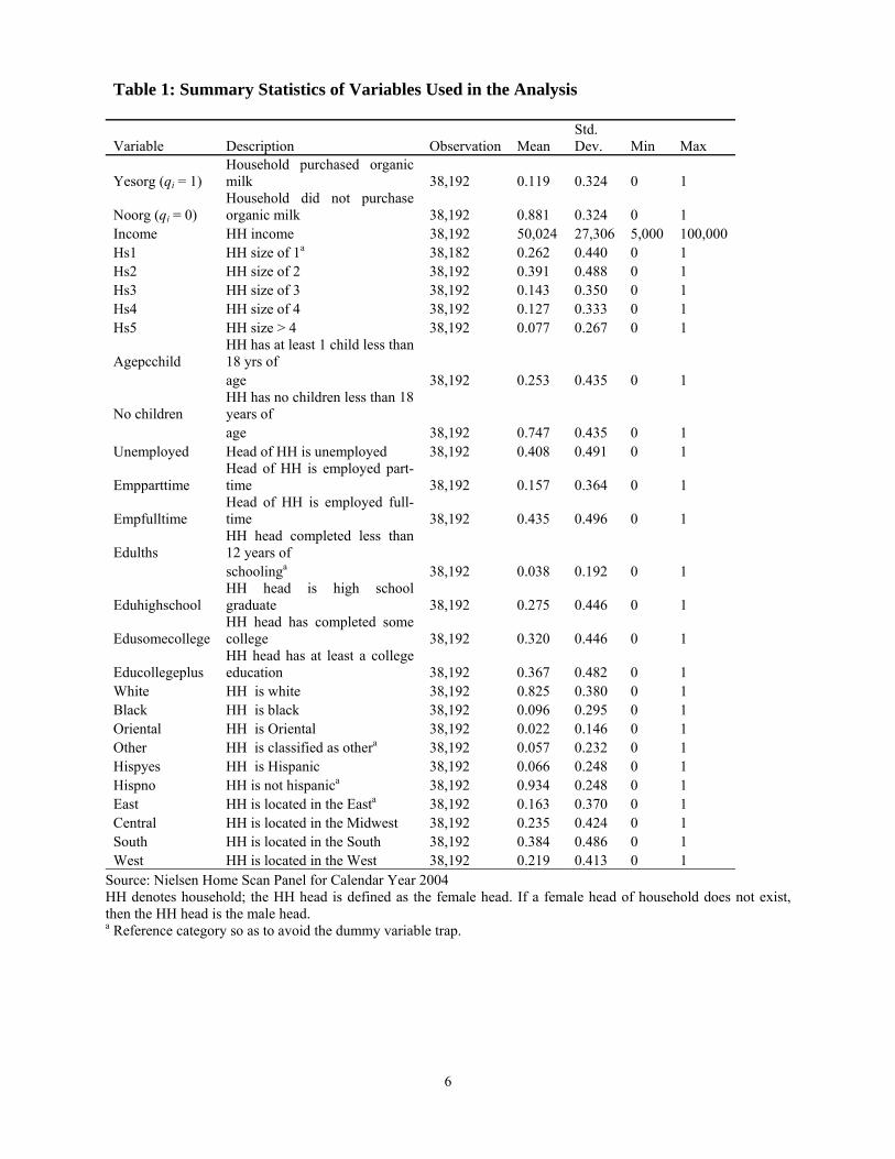
Table 1: Summary Statistics of Variables Used in the Analysis

Variable Description Observation Mean Std. Dev. Min Max

Yesorg (qi = 1)

Household purchased organic milk 38,192 0.119 0.324 0 1

Noorg (qi = 0) Household did not purchase organic milk 38,192 0.881 0.324 0 1

Income HH income 38,192 50,024 27,306 5,000 100,000 Hs1 HH size of 1a 38,182 0.262 0.440 0 1 Hs2 HH size of 2 38,192 0.391 0.488 0 1 Hs3 HH size of 3 38,192 0.143 0.350 0 1 Hs4 HH size of 4 38,192 0.127 0.333 0 1 Hs5 HH size > 4 38,192 0.077 0.267 0 1

Agepcchild HH has at least 1 child less than 18 yrs of

age 38,192 0.253 0.435 0 1

No children HH has no children less than 18 years of

age 38,192 0.747 0.435 0 1 Unemployed Head of HH is unemployed 38,192 0.408 0.491 0 1

Empparttime Head of HH is employed part-time 38,192 0.157 0.364 0 1

Empfulltime Head of HH is employed full-time 38,192 0.435 0.496 0 1

Edulths HH head completed less than 12 years of

schoolinga 38,192 0.038 0.192 0 1

Eduhighschool HH head is high school graduate 38,192 0.275 0.446 0 1

Edusomecollege HH head has completed some college 38,192 0.320 0.446 0 1

Educollegeplus HH head has at least a college education 38,192 0.367 0.482 0 1

White HH is white 38,192 0.825 0.380 0 1 Black HH is black 38,192 0.096 0.295 0 1 Oriental HH is Oriental 38,192 0.022 0.146 0 1 Other HH is classified as othera 38,192 0.057 0.232 0 1 Hispyes HH is Hispanic 38,192 0.066 0.248 0 1 Hispno HH is not hispanica 38,192 0.934 0.248 0 1 East HH is located in the Easta 38,192 0.163 0.370 0 1 Central HH is located in the Midwest 38,192 0.235 0.424 0 1 South HH is located in the South 38,192 0.384 0.486 0 1 West HH is located in the West 38,192 0.219 0.413 0 1

Source: Nielsen Home Scan Panel for Calendar Year 2004 HH denotes household; the HH head is defined as the female head. If a female head of household does not exist, then the HH head is the male head. a Reference category so as to avoid the dummy variable trap.

7

Equation (17) omits everything except for the income covariate. We use this specification to determine the impact of censoring potentially important socio-demographic variables on the forecasting ability of binary choice models. Thus, two sets of predicted probabilities for each choice model (probit, logit and LPM) were estimated. These in turn were used to derive two sets of Brier Scores, prediction success tables, and Yates Brier Score partition (decomposition) factors.

DATA For this empirical exercise, the data pertaining to the choice of purchasing organic milk, income and household socio- demographic variables are from the 2004 Nielsen Homescan Panel. Table 1 presents the definition and summary statistics of all the relevant variables that were used in the study. The Nielsen Panel is an on-going scanner data survey system, tracking household purchases in the United States.

The variable Yesorg is the dependent choice variable and is indexed as 1 to represent purchase of organic milk and 0 otherwise. Income is defined as household income and the average income level of the sample was $50,025/household. As for the household size, the study used indicator variables to describe the number of household members where Hs1 (26%) and Hs2 (40%) pertain to households having one and two members, while hs3 has three household members with a mean proportion of 14 percent. The two last household size indicator variables hs4 and hs5 describes four and five or more members in the household. The respective mean proportions are 13 and 8 percent respectively Also, households with children less than 18 years old (agepcchild) were 25 percent of the sample. The demographic characteristics of the household head also were included in this study. Both the employment status and educational attainment of the household head were represented as dummy or indicator variables. The variables Unemp, Empparttime and Empfulltime are indicator variables representing the employment status of the household head, eitherunemployed, employed part-time or employed fulltime. Their respective mean proportions are 41 percent, 16 percent and 43 percent. Similarly the variables Edulths, Eduhighschool, Edusomecollege and Educollege denote household head educational attainment whether it is below high school, high school, above high school but below college and college and beyond. The respective mean proportions are 4 percent, 28 percent, 32 percent and 37 percent. Also included into the respective model specification were race and ethnicity of the household. The indicator variables White, Black, Oriental and Others represented the major racial household distinction. Approximately 83 percent are white households. On the other hand household ethnicity was represented as either Hispanic (Hispyes-7 percent) or non-Hispanic (Hispno-93 percent). Finally, regional dummy variables such as East, Central, South and West were included to describe the regional location of the household. The respective mean proportions are 16 percent, 24 percent, 38 percent and 22 percent respectively.

8

RESULTS

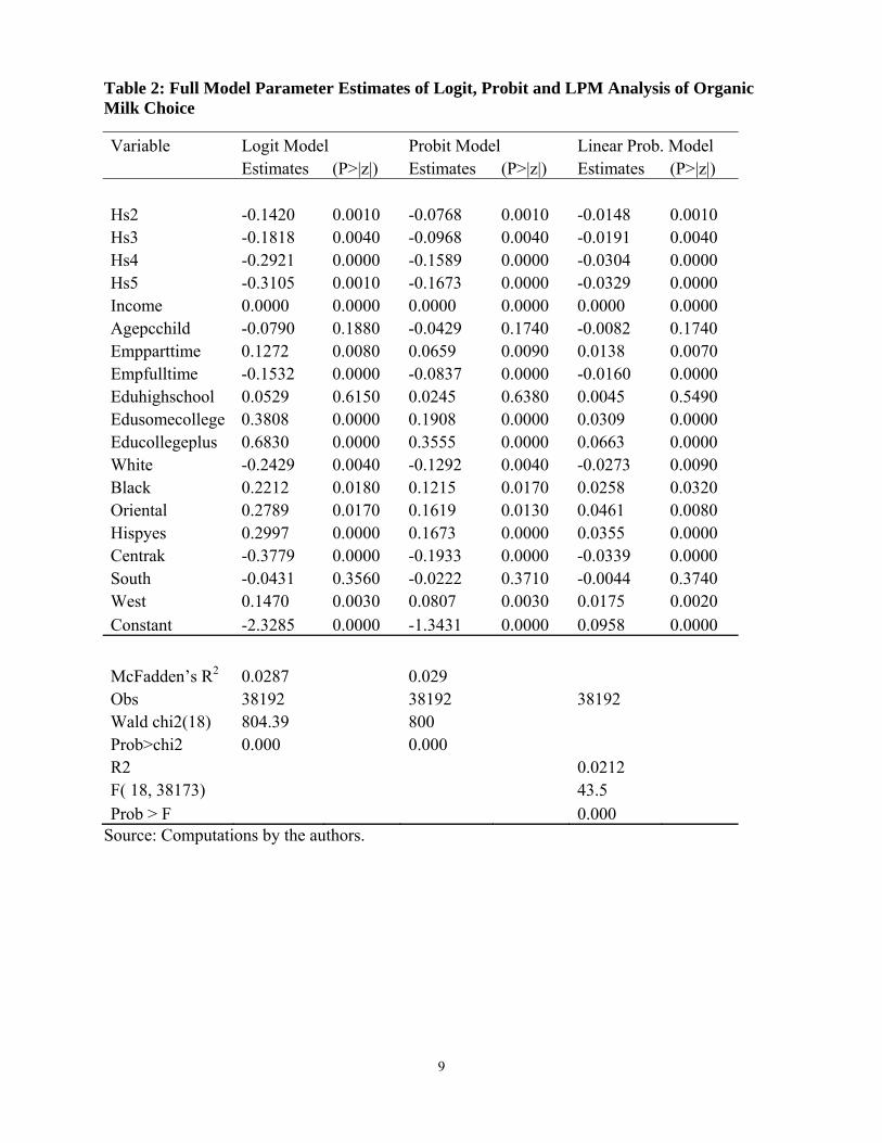
Inter-Binary Choice Model Comparisons For this exercise, three models were used, namely the probit, logit and linear probability models to represent the binary choice between organic and conventional milk. Tables 2 and 3 report the logit, probit and LPM estimated parameters of both the full model and income only model. The Brier Score and Yates partition components are exhibited in Table 4. The calculated Brier Scores (BS) for the three respective models are given as follows: probit (BS=0.1028960), logit (BS=0.1029092) and LPM (BS=0.1028963). Furthermore, the probit model has the highest forecast covariance value compared to the other two models. These results imply that the probit model predicts better than the logit and LPM models by having both the lowest Brier scores and highest forecast covariance values (Table 4). Prediction success tables also were utilized to assess the ability of the “complete” model to classify outcomes (Table 5). Instead of the default 0.5 cut-off value, the appropriate critical values were calculated based on the purchase frequency of organic milk relative to the whole sample size. The choice of cut-off value was made to reflect the actual probability of choosing organic milk and not the usual application of the equal odds approach in both choices. For all three choice models utilized, the cutoff value was equal to 0.119. Results indicate that the logit model garnered the highest percentage of right predictions (58.41 percent) relative to the probit (57.97 percent) and the LPM (54.64 percent). The implication is that the logit model results in 58 percent correct predictions, the probit just fewer than 58 percent correct predictions, and the LPM slightly more than 54 percent correct predictions. Thus, among the three models, the logit model performs best in correctly classifying those households that chose organic and/or conventional milk.

Inter-Model Probabilistic Graphs Following Yates (1982, 1988) and Olvera and Bessler (2006), illustrative constructs called probabilistic or covariance graphs were utilized to demonstrate the ability to differentiate binary choice events that had occurred or did not occur. The graphs illustrate the ability to discriminate between the choice of purchasing organic and conventional milk across three binary choice models, namely probit, logit and linear probability models (LPM). Results indicate that the slope and intercept of the three probabilistic graphs (Figures 1a, 2a and 3a) have values that are close to one another.

Intra-Binary Choice Model Comparisons In this section, the analysis shifts from comparing different binary choice models to looking at one choice model and its respective model variant. More specifically, we compare a choice model containing covariates such as income and various socio-demographic variables with a model variant which contains income as its only explanatory variable.

9

Table 2: Full Model Parameter Estimates of Logit, Probit and LPM Analysis of Organic Milk Choice

Variable Logit Model Probit Model Linear Prob. Model Estimates (P>|z|) Estimates (P>|z|) Estimates (P>|z|) Hs2 -0.1420 0.0010 -0.0768 0.0010 -0.0148 0.0010 Hs3 -0.1818 0.0040 -0.0968 0.0040 -0.0191 0.0040 Hs4 -0.2921 0.0000 -0.1589 0.0000 -0.0304 0.0000 Hs5 -0.3105 0.0010 -0.1673 0.0000 -0.0329 0.0000 Income 0.0000 0.0000 0.0000 0.0000 0.0000 0.0000 Agepcchild -0.0790 0.1880 -0.0429 0.1740 -0.0082 0.1740 Empparttime 0.1272 0.0080 0.0659 0.0090 0.0138 0.0070 Empfulltime -0.1532 0.0000 -0.0837 0.0000 -0.0160 0.0000 Eduhighschool 0.0529 0.6150 0.0245 0.6380 0.0045 0.5490 Edusomecollege 0.3808 0.0000 0.1908 0.0000 0.0309 0.0000 Educollegeplus 0.6830 0.0000 0.3555 0.0000 0.0663 0.0000 White -0.2429 0.0040 -0.1292 0.0040 -0.0273 0.0090 Black 0.2212 0.0180 0.1215 0.0170 0.0258 0.0320 Oriental 0.2789 0.0170 0.1619 0.0130 0.0461 0.0080 Hispyes 0.2997 0.0000 0.1673 0.0000 0.0355 0.0000 Centrak -0.3779 0.0000 -0.1933 0.0000 -0.0339 0.0000 South -0.0431 0.3560 -0.0222 0.3710 -0.0044 0.3740 West 0.1470 0.0030 0.0807 0.0030 0.0175 0.0020 Constant -2.3285 0.0000 -1.3431 0.0000 0.0958 0.0000

McFadden’s R2 0.0287 0.029 Obs 38192 38192 38192 Wald chi2(18) 804.39 800 Prob>chi2 0.000 0.000 R2 0.0212 F( 18, 38173) 43.5 Prob > F 0.000

Source: Computations by the authors.

10

Table 3: Income-Only Model Parameter Estimates of Logit, Probit and LPM Analysis of Organic Milk Choice

Variable Logit Model Probit Model Linear Prob. Model Estimates (P>|z|) Estimates (P>|z|) Estimates (P>|z|) Income 7.34E-06 0.0000 3.88E-06 0.0000 7.89E-07 0.0000 Constant -2.38081 0.0000 -1.3788 0.0000 0.079893 0.0000

McFadden’s R2 0.0059 0.0059 Obs 38192 38192 38192 Wald chi2(1) 165.54 164.12 Prob>chi2 0.0000 0.0000 R2 0.0044 F( 1, 38190) 156.94 Prob > F 0.0000

Source: Computations by the authors. Results from Table 4 indicate that for all three models, Brier scores had increased between complete models and their variants with income as the only explanatory variable. More specifically, the increase in terms of percent change for the probit versus probit variant (income only) model was approximately 1.71 percent. For the logit model and its respective logit variant, the percent change increased by 1.69 percent. As for the LPM and model variant, the approximate increase in percentage change was 1.71 percent. The increase in the Brier scores implies diminishing forecasting ability of all three models with respect to predicting both choices (Table 4). This difference in Brier score was brought about by the declining variability of the predicted probabilities due to the omission of critical socio-demographic variables in a binary choice model specification (MinVar(p)). Thus, the results imply that when important socio-demographic determinants are removed, the variability of predicted probabilities is reduced and therefore forecasting ability is diminished. Results from the prediction success-tables exhibited in Table 5 indicate that for both probit and logit models, the percent of right predictions declined by approximately 2.27 percent and 3 percent. As for the LPM model, percentage of right predictions increased by 3.69 percent. Also for both the probit and logit models, we find that in terms of sensitivity or the ability to classify correctly the choice of organic milk, the sensitivity declined by 15.58 percent and 14.82 percent. Likewise, the specificity, or the ability to correctly predict the choice of conventional milk, declined by 0.36 percent and 1.34 percent among model variants. The sensitivity of the LPM decreased by 21 percent while its specificity increased by 7.77 percent. Again based on the results of the prediction-success or contingency tables, censure of critical important socio-demographic variables reduces in most cases the ability of choice models to make right predictions.

11

Table 4: Brier Score and Decompositions of Probit, Logit and Linear Probability Model (LPM) and Model Variants for Organic Milk Choice

PROBIT MODEL Probit Probit % Change

(Full Model) (Income Only)a Brier Score (BS) 0.1028960 0.1046501 1.705 Variance of d (Var(d)) 0.1051212 0.1051212 0.000 Minimum variance of p (Min Var(p)) 0.0000487 0.0000020 -95.873 Scatter (Scatter(p)) 0.0022488 0.0004615 -79.478

Bias2 1.1E-10 8.1E-13 -99.264 Forecast covariance (2Cov(p,d)) 0.0045228 0.0009346 -79.336

Slope 0.0215121 0.0044453 -79.336 Intercept 0.1167921 0.1188407 1.754 LOGIT MODEL Logit Logit % Change (Full Model) (Income Only) Brier Score (BS) 0.1029092 0.1046490 1.691 Variance of d (Var(d)) 0.1051212 0.1051212 0.000 Minimum variance of p (Min Var(p)) 0.0000484 0.0000015 -96.921 Scatter (Scatter(p)) 0.0022520 0.0004645 -79.374

Bias2 0.0000000 0.0000000 0.000 Forecast covariance (2Cov(p,d)) 0.0045124 0.0009388 -79.195

Slope 0.0214629 0.0044655 -79.194 Intercept 0.1168085 0.1188375 1.737 LINEAR PROBABILITY MODEL LPM LPM % Change (Full Model) (Income Only) Brier Score (BS) 0.1028963 0.1046569 1.711 Variance of d (Var(d)) 0.1051212 0.1051212 0.000 Minimum variance of p (Min Var(p)) 0.0000471 0.0000021 -95.520 Scatter (Scatter(p)) 0.0021779 0.0004623 -78.773

Bias2 0.0000000 0.0000000 0.000 Forecast covariance (2Cov(p,d)) 0.0044500 0.0009288 -79.128

Slope 0.0211657 0.0044175 -79.129 Intercept 0.1168440 0.1188432 1.711 a Model variant has income as the only explanatory variable for all the three choice models.

Source: Computations by the authors.

12

Table 5: Prediction-Success Evaluation for Probit, Logit and Linear Probability Models (LPM) in Both Full Model and Income-only Specifications PROBIT Actual Choice

Complete Income Only

Predictions Organic Milk Conventional Organic Milk Conventional

Organic Milk 2772 14266 2340 14336

Conventional 1787 19367 2219 19297

Total 4559 33633 4559 33633

Full Model Income Only

% Right Predictionsa 57.97 56.65

Sensitivity (%)b 60.80 51.33

Specificity (%)c 57.58 57.38

Cut-off value 0.12 0.12

LOGITd Actual Choice



Organic Milk 2747 14073 2340 14336

Conventional 1812 19560 2219 19297

Total 4559 33633 4559 33633


% Right Predictions 58.41 56.65

Sensitivity (%) 60.25 51.33

Specificity (%) 58.16 57.38 Cut-off value 0.12 0.12

LPMe Actual Choice



Organic Milk 2962 15727 2340 14336

Conventional 1597 17906 2219 19297

Total 4559 33633 4559 33633


% Right Predictions 54.64 56.65

Sensitivity (%) 64.97 51.33

Specificity (%) 53.24 57.38

Cut-off value 0.12 0.12 a For full model ((2772+19367)/38192)*100 and for income only ((2340+19297)/38192)*100 b Corresponds to the percentage of correctly predicting the choice of choosing organic milk. For full model (2772/4559)*100 and for income only (2340/4559)*100 c Corresponds to the percentage of correctly predicting the choice of choosing conventional milk. For full model (19367/33633)*100 and for income only (19297/33633)*100 d, e Same calculations as with the probit example Source: Computations by the authors.

13

Figure 1: Probit (a) and Probit-Income Variant (b) Model Probabilistic Graphs

(a)

(b)

0.1

.2.3

.4O

rgan

ic M

ilk C

hoic

e F

orec

ast

0 .2 .4 .6 .8 1Outcome Index

Fitted values Model Issued Prob.

14

Figure 2: Logit (a) and Logit-Income Variant (b) Model Probabilistic Graphs

(a)

(b)

0.1

.2.3

.4O

rgan

ic M

ilk C

hoic

e F

orec

ast



0.1

.2.3

.4O

rgan

ic M

ilk C

hoic

e F

orec

ast



15

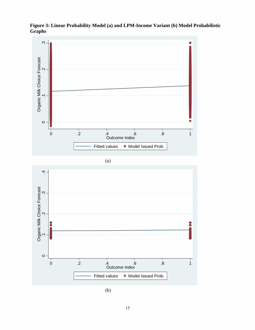
Figure 3: Linear Probability Model (a) and LPM-Income Variant (b) Model Probabilistic Graphs

(a)

(b)

0.1

.2.3

Org

anic

Milk

Cho

ice

For

ecas

t



0.1

.2.3

.4O

rgan

ic M

ilk C

hoic

e F

orec

ast



16

Intra-Model Probabilistic Graphs Figures 1a, 1b, 2a, 2b, 3a and 3b illustrate pairwise covariance graphs for probit, logit, LPM specifications and their respective model variants. Results show that the slopes of the probit, logit and LPM covariance graphs declined significantly when socio-demographic variables were removed from the original binary choice specification. For example, percentage changes in the slope for the probit and its income-only variant declined by approximately 79 percent. For the logit and LPM models, the percentage change in slope also decreased by 79 percent. These numbers are confirmed by the flatter probabilistic graphs that characterize choice models that are income-only variants.

Intra-Model Analysis of the Yates Partition The Yates partition decomposes the Brier score into factors such as bias, scatter, minimum forecast variance, variance of outcome index (d) and covariance between p and d. In this section we center attention to the effect on scatter and minimum variance components. Results from Table 4 show that across the three models, the values of both factors declined noticeably when the number of explanatory variables were reduced to only the income variable. For example, the declining percent change for the probit model and its income only variant in both minimum forecast variance and scatter were 95.87 percent and 79.48 percent. Likewise, for the logit model and its income-only model variant, the decline in percentage change were approximately 96.92 (minimum forecast variance) and 79.37 percent (scatter). As for the LPM model, similar changes also were observed in both direction of change and magnitude relative to the probit and logit models. The effect of omitting important socio-demographic variables resulted then in reducing the variability of predicted probabilities. This reduction however also can mean limited information flow which can constrain the ability of choice models to discriminate between events that occurred and those that did not occur. With limited information flow, we find that there is increased filtering of irrelevant information, and therefore the value of the scatter component decreases. As with the minimum variance, the limited information reduced the overall variance of the respective probabilities. Finally, with reduced information flow, the gap between probabilities assigned to binary events diminishes, thus we find that the forecast covariance decreases. In summary, model specifications that limit information flow in binary choice models can bring about increased noise filtering (declining scatter), lessening of overall forecast variance (decreased minimum forecast variance) and weakening of the ability to filter relevant information that enables the proper assignment of probabilities for events that occur and did not occur (reduced forecast covariance).

CONCLUSIONS There were two levels of analysis done in this study, namely considering comparisons across choice models and considering comparisons of alternative specifications within choice models. Utilizing probit, logit and linear probability choice models to represent the choice of organic milk or conventional milk, both Brier scores and prediction-success tables were evaluated to

17

determine their usefulness in making accurate predictions. Results indicated that the probit model predicted better among the three models by having the lowest Brier Score and highest forecast covariance values. However, when the prediction-success criterion was used, the logit model performed best in terms of correct classifications. One notable observation was that across the three models, the values of the Brier score, Yates partition factors and prediction-success tables were very close in magnitude. The study also utilized probabilistic graphs in order to illustrate the ability of all models to differentiate between events that occurred (choosing organic milk) and those that did not occur (choosing conventional milk). When important socio-demographic variables were omitted in the binary choice models, the variability level of the predicted probabilities was notably reduced. Consequently, the ability of the model to sort binary events or choices was diminished. Estimates from the Brier scores indicated that for each of the choice models vis-à-vis their respective income-only variant, the values increased indicating diminished forecasting ability. Likewise, results from the prediction-success table pointed to declining percentages of correct classifications. The declining slope change of the covariance graphs between “complete” models and their income-only variants was indicative of diminished binary event discriminatory ability. With regard to the effect on the factors from the Yates partition, the study focused on the scatter and minimum variance. Results showed that when socio-demographic variables were omitted, scatter and minimum variance values were reduced. An intuitive explanation for this change lies in the reduction of the variability of predicted probabilities. Also, the removal of socio-demographic variables resulted in a weakened ability to sort between events that occurred and did not occur. As to the use of prediction-success tables, analysts should also utilize other methods such as probability scoring to get a more complete picture of the ability of the binary choice model in question.

18

REFERENCES Alviola IV, P., Capps, Jr., O.(2009). Household Demand Analysis of Organic and Conventional

Fluid Milk in the United States Based on the 2004 Homescan Panel. Dept. of Agricultural Economics, Texas A&M University, Research Report.

Bessler, D.A., Ruffley, R. (2004). Prequential Analysis of Stock Market Returns. Applied Economics 36: 399-412.

Cameron, A.C., Trivedi, P.K. (2005). Microeconometrics: Methods and Applications. New York: Cambridge University Press.

Cameron, A.C., Trivedi, P.K. (2008). Microeconometrics using STATA. STATA Press, StataCorps LP, College Station, Texas.

Capps, Jr. O., Kramer, R.A.(1985). Analysis of Food Stamp Participation Using Qualitative Choice Model. American Journal of Agricultural Economics 67: 49-59.

Olvera, G.C.,. Bessler, D.A. (2006). Probability Forecasting and Central Bank Accountability. Journal of Policy Modeling 28: 223-234.

Park, J. and Capps, Jr. O. (1997). The Demand for Prepared Meals by US Households. American Journal of Agricultural Economics 79: 814-824.

Stock J. H., Watson, M.W. (2007). Introduction to Econometrics. Boston Massachusetts: Pearson-Addison Wesley.

Wooldridge, J. (2002). Econometric Analysis of Cross Section and Panel Data Method. Cambridge, Massachusetts: The MIT Press.

Yates, F.T. (1982). External correspondence: Decomposition of the Mean Probability Score. Organizational Behavior and Human Performance 30: 132-156.

Yates, F.T. (1988). Analyzing Accuracy of Probability Judgments for Multiple Events: An Extension of the Covariance Decomposition. Organizational Behavior and Human Performance 41: 281-299.

Documents

THE IMPORTANCE OF SOCIO DEMOGRAPHIC VARIABLES ON …afcerc.tamu.edu/publications/Publication-PDFs/CP-02-09_BrierProbitProbabilityOrganic...THE IMPORTANCE OF SOCIO DEMOGRAPHIC VARIABLES