1

The Impacts of Congestion on Time-definitive Urban Freight Distribution Networks CO2 Emission Levels: results from a case study in Portland,

Oregon

Miguel Andres Figliozzi Associate Professor

Department of Civil and Environmental Engineering Portland State University

P.O. Box 751, Portland, OR 97207-0751 Email: figliozzi@pdx.edu

Abstract

Increased congestion during peak morning and afternoon periods in urban areas is increasing logistics costs. In addition, environmental, social, and political pressures to limit the impacts associated with CO2 emissions are mounting rapidly. A key challenge for transportation agencies and businesses is to improve the efficiency of urban freight and commercial vehicle movements while ensuring environmental quality, livable communities, and economic growth. However, research and policy efforts to analyze and quantify the impacts of congestion and freight public policies on CO2 emissions are hindered by the complexities of vehicle routing problems with time-dependent travel times and the lack of network-wide congestion data. This research focuses on the analysis of CO2 emissions for different levels of congestion and time-definitive customer demands. Travel time data from an extensive archive of freeway sensors, time-dependent vehicle routing algorithms, and problems-instances with different types of binding constraints are used to analyze the impacts of congestion on commercial vehicle emissions. Results from the case study indicate that the impacts of congestion or speed limits on commercial vehicle emissions are significant but difficult to predict since it is shown that it is possible to construct instances where total route distance or duration increases but emissions decrease. Public agencies should carefully study the implications of policies that regulate depot locations and travel speeds as they may have unintended negative consequences in terms of CO2 emissions.

KEYWORDS: Vehicle routing, time dependent travel time-speed, GHG or CO2 emissions, urban congestion, depot location.

Submitted: December 2009 Submitted 2nd revision, December 2010

2

1. Introduction

Urban freight is responsible for a large share, or in some cities the largest share, of unhealthy

air pollution in terms of sulphur oxide, particulate matter, and nitrogen oxides in urban areas

such as London, Prague, and Tokyo (OECD, 2003, Crainic et al., 2009). The fast rate of

commercial vehicle activity growth over recent years and the higher impact of commercial

vehicles (when compared to passenger vehicles) are increasing preexisting concerns over their

cumulative effect in urban areas. In particular, environmental, social, and political pressures

to limit the impacts associated with carbon dioxide (CO2) emissions and fossil fuel

dependence are mounting rapidly.

A key challenge for transportation agencies is to improve the efficiency of urban freight and

commercial vehicle movements while ensuring environmental quality, livable communities,

and economic growth. Research in the area of city logistics has long recognized the need for a

balanced approach to reduce shippers’ and carriers’ logistics cost as well as community’s

traffic congestion and environmental problems (Taniguchi et al., 2003, Crainic et al., 2004).

Although past and current research efforts into vehicle routing algorithms and scheduling are

extensive (Cordeau et al., 2006) most research efforts have ignored freight-related

environmental and social externalities. Furthermore, the body of research devoted to

investigating the impacts of congestion on urban commercial vehicle operations and time-

dependent travel times is relatively scant. In the existing literature, there are no published

congestion case studies involving CO2 emission levels, time-dependent vehicle routing

problems, and a diverse set of customer constraints.

This research focuses on the analysis of CO2 emissions for different levels of time-definitive

customer demands using congestion data from an extensive archive of freeway and arterial

streets and a time-dependent vehicle routing (TDVRP) solution method to design commercial

vehicle routes. To the best of the author’s knowledge, there is no published research on the

impacts of congestion, land use, and travel speeds on CO2 emissions for commercial vehicle

routing in networks with time-dependent travel speeds, hard time windows, and real-world

time/distance data.

3

This research is organized as follows: Section 2 provides the necessary background and a

literature review. Section 3 presents the mathematical formulation of the time-dependent hard

time windows routing problem as well as an expression to calculate CO2 emissions. Section 4

describes the Portland case study, its data sources, and the solution approach. Section 5

presents and analyzes experimental results. Section 6 ends with conclusions.

2. Background and Literature Review

The literature review for this paper covers three main areas of research: (a) the effects of

congestion and travel time variability on vehicle tours and logistics; (b) the impact of travel

speeds on commercial vehicle emissions; and (c) time-dependent vehicle routing problems.

Direct and indirect costs of congestion on passenger travel time, shipper travel time and

market access, production, and labor productivity have been widely studied and reported in

the available literature. The work of Weisbrod et al. (2001) provides a broad review of this

literature. Survey results suggest that the type of freight operation has a significant influence

on how congestion affects carriers’ operations and costs. For example, results from a

California survey indicate that congestion is perceived as a serious problem for companies

specializing in less-than-truckload (LTL), refrigerated, and intermodal cargo (Golob and

Regan, 2001). These results largely agree with reports analyzing the effects of traffic

congestion in the Portland region (ERDG, 2005, 2007).

Congestion has a significant impact on routes where delivery times are heavily restricted by

customer time windows and schedules. In addition, there may be a fairly inelastic relationship

between delivery costs and customer’s demand characteristics and levels. For example,

Holguin-Veras et al. (2006) investigated the effects of New York City’s congestion pricing on

LTL deliveries and found little changes because delivery times were determined by customer

time windows and schedules. Figliozzi (2007, 2009a) analyzes the effects of congestion on

vehicle tour characteristics using continuous approximations to routing problems. Figliozzi

(2007) analyzes how constraints and customer service time affect trip generation using a tour

classification based on supply chain characteristics and route constraints. This work also

reveals that changes in both vehicle kilometers traveled (VKT) and vehicle hours traveled

(VHT) differ by type of tour and routing constraint. Hard time windows are the type of

constraint that most severely increases VKT and VHT. Figliozzi (2009a) models the effects of

congestion and travel time variability on vehicle tour characteristics; analytical and numerical

4

results indicate that travel speed reductions and depot-customer travel distances are the key

factors that exacerbate the impacts of travel time variability. Quak and Koster (2009) utilized

a fractional factorial design and regression analysis to quantify the impacts of delivery

constraints and urban freight policies. Quak and Koster (2009) findings confirm previous

results. Vehicle restrictions that affected customers with time window constraints did not have

an impact on customer costs. However, vehicle restrictions are found to be costly when

vehicle capacity is limited.

There is an extensive literature related to vehicle emissions and several laboratory and field

methods are available to estimate vehicle emissions rates (Ropkins et al., 2009). Research

results indicate that CO2 is the predominant transportation greenhouse gas (GHG) and is

emitted in direct proportion to fuel consumption, with a variation by type of fuel (ICF, 2006).

For most vehicles, fuel consumption and the rate of CO2 per mile traveled decreases as

vehicle operating speed increases up to an optimal speed and then begins to increase again

(ICF, 2006). Furthermore, the relationship between emission rates and travel speed is not

linear.

Congestion has a great impact on CO2 vehicle emissions and fuel efficiency. In real driving

conditions, there is a rapid non-linear growth in emissions and fuel consumption as travel

speeds fall below 30 mph (Barth and Boriboonsomsin, 2008). CO2 emissions double on a per

mile basis when speed drops from 30 mph to 12.5 mph or when speed drops from 12.5 mph to

5 mph. These results were obtained using an emission model and freeway sensor data in

California and weighted on the basis of a typical light-duty fleet mix in 2005. Frequent

changes in speed, i.e. stop and go traffic conditions, increases emission rates because fuel

consumption is a function of not only speed but also acceleration rates (Frey et al., 2008).

Some researchers have conducted surveys that indicate that substantial emission reductions

can be obtained if companies improve the efficiency of routing operations (Léonardi and

Baumgartner, 2004, Baumgartner et al., 2008). Other researchers using queuing theory,

Woensel et al. (2001) modeled the impact of traffic congestion on emissions and recommend

that private and public decision makers take into account the high impact of congestion on

emissions. From an operational perspective, carriers cannot take into account the impact of

congestion on emissions unless time-dependent travel times are considered when designing

distribution or service routes. While classic versions of the VRP, specifically the capacitated

VRP (CVRP) or VRP with time windows (VRPTW), have been widely studied in the

5

available literature (Cordeau et al., 2006), time-dependent problems have received

considerably less attention. The Time Dependent Vehicle Routing Problem (TDVRP) takes

into account that links in a network have different costs or speeds during the day. Typically,

this time-dependency is used to represent varying traffic conditions. The TDVRP was

originally formulated by Malandraki and Daskin (1992). Time dependent models are

significantly more complex and computationally demanding than static VRP models.

Approaches to solve the TDVRP can be found in the work of several authors (Malandraki,

1989, Ahn and Shin, 1991, Jung and Haghani, 2001, Ichoua et al., 2003, Fleischmann et al.,

2004, Haghani and Jung, 2005, Donati et al., 2008, Figliozzi, 2009c). The reader is referred to

Figliozzi (2009c) for an up-to-date and extensive TDVRP literature review and the

description of benchmark problems.

TDVRP instances are considerably more demanding than static VRP instances in terms of

data requirements and computational time. However, solving more realistic TDVRP instances

may indirectly achieve environmental benefits in congested areas because total route

durations and distances can be reduced even though emissions are not part of the objective

function (Sbihi and Eglese, 2007). Though the emissions problem is complex; as shown in

Section 5, it is possible to construct instances where distance or duration increases but

emissions decrease. Palmer (2008) studied the minimization of CO2 emissions utilizing real

network data, multi-stop routes averaging almost 10 deliveries per route, and shortest paths of

Surrey county in the U.K. However, Palmer’s methodology does not allow for time-dependent

speeds or multi-stop routes. Figliozzi (2010) formulated the emissions vehicle routing

problem (EVRP) with time-dependent travel times, hard time windows, and capacity

constraints. In addition to the usual binary variables for assigning vehicles to customers, this

is the first VRP with time windows formulation to include speed and departure time as

decision variables and also present conditions and algorithms to determine efficient departure

times and travel speeds. Figliozzi (2010) showed that a routing formulation and solution

algorithm that takes into account congestion and aims to minimize CO2 emissions can

produce significant reductions in emission levels with relatively small increases in distance

traveled or fleet size.

To the best of the author’s knowledge, there is no published work simultaneously integrating

in a case study problems with time-dependent speeds, distinct depot locations, hard time

windows, real-world network and congestion data, and commercial vehicles emissions.

6

3. Notation and Problem Formulation

Unlike the formulation presented by Figliozzi (2010), in this research travel speeds are not

optimized to reduce emissions but introduced as decision variables to represent restrictions

due to freight policy measures, congestion, or time windows. Hence, carriers in this research

continue “business as usual” without internalizing the costs of emissions.

Using a traditional flow-arc formulation (Desrochers et al., 1988) and building upon a

formulation of the TDVRP with time windows (Figliozzi, 2009b)b), the vehicle routing

problem studied in this research can be described as follows. Let ( , )G V A= be a graph where

{( , ) : , }i jA v v i j i j V= ≠ ∧ ∈ is an arc set and the vertex set is 0 1( ,...., )nV v v += . Vertices 0v

and 1nv + denote the depot at which vehicles of capacity maxq are based. Each vertex in V

has an associated demand 0iq ≥ , a service time 0ig ≥ , and a service time window [ , ]i ie l ; in

particular the depot has 0 0g = and 0 0q = . The set of vertices 1{ ,...., }nC v v= specifies a set of

n customers. The arrival time of a vehicle at customer ,i i C∈ is denoted ia and its departure

time ib . Each arc ( , )i jv v has an associated constant distance 0i jd ≥ and a travel time

( ) 0i j it b ≥ which is a function of the departure time from customer i . The set of available

vehicles is denoted K . The cost per unit distance traveled is denoted dc . A binary decision

variable kijx indicates whether vehicle k travels between customers i and j . A real decision

variable kiy indicates service start time if customer i is served by vehicle k ; hence the

departure time is given by the customer service start time plus service time ki i ib y g= + .

In the capacitated vehicle routing problem with time windows (VRPTW) it is traditionally

assumed that carriers minimize the number of vehicles as a primary objective and distance

traveled as a secondary objective without violating time windows, route durations, or capacity

constraints. The problem analyzed in this research follows this traditional approach; however,

CO2 emissions are also computed to analyze emissions tradeoffs due to policy restrictions,

time windows, or congestion levels.

Problem Formulation

The primary objective is fleet size minimization as defined by (1) and the secondary objective

is the minimization of distance traveled and route duration costs.

7

PRIMARY OBJECTIVE

0k

jk K j C

minimize x∈ ∈∑∑ , (1)

SECONDARY OBJECTIVE

( , )

kd ij ij

k K i j Vminimize c d x

∈ ∈∑ ∑ (2)

CONSTRAINTS

maxk

i iji C j V

q x q∈ ∈

≤∑ ∑ , k K∀ ∈ (3)

1kij

k K j V

x∈ ∈

=∑∑ , i C∀ ∈ (4)

0k kil lj

i V i V

x x∈ ∈

− =∑ ∑ , ,l C k K∀ ∈ ∀ ∈ (5)

0 1,0, 0k ki n ix x += = , ,i V k K∀ ∈ ∀ ∈ (6)

0 1kj

j Vx

∈

=∑ , k K∀ ∈ (7)

, 1 1kj n

j Vx +

∈

=∑ , k K∀ ∈ (8)

k ki ij i

j Ve x y

∈

≤∑ , ,i V k K∀ ∈ ∀ ∈ (9)

k ki ij i

j Vl x y

∈

≥∑ , ,i V k K∀ ∈ ∀ ∈ (10)

, ,( ( ))k k k ki j i i i j i i jx y g t y g y+ + + ≤ , ( , ) ,i j A k K∀ ∈ ∀ ∈ (11)

{0,1}kijx ∈ , ( , ) ,i j A k K∀ ∈ ∀ ∈ (12)

kiy ∈ℜ , ,i V k K∀ ∈ ∀ ∈ (13)

The constraints are defined as follows: vehicle capacity cannot be exceeded (3); all customers

must be served (4); if a vehicle arrives at a customer it must also depart from that customer

8

(5); routes must start and end at the depot (6); each vehicle leaves from and returns to the

depot exactly once, (7) and (8) respectively; service times must satisfy time window start (9)

and ending (10) times; and service start time must allow for travel time between customers

(11). Decision variables type and domain are indicated in (12) and (13).

Emissions Modeling

CO2 emissions are proportional to the amount of fuel consumed which is a function of travel

speed and distance traveled among other factors. In this research it is assumed that the weight

of the products loaded does not significantly affect CO2 emission levels in relation to the

impacts of travel speeds. To incorporate recurrent congestion impacts and following a

standard practice in TDVRP models, the depot working time 0 0[ , ]e l is partitioned into M

time periods 1 1, , ..., MT T T=T ; each period mT has an associated constant travel speed 0 ms≤

in the time interval [ , ]m m mT t t= .

For each departure time ib and each pair of customers i and j , a vehicle travels a non-

empty set of speed intervals 1( ) { ( ), ( ),..., ( )}m m m pij i ij i ij i ij iS b s b s b s b+ += where ( )m

ij is b denotes the

speed at departure time, ( )m pij is b+ denotes the speed at arrival time, and 1p + is the number of

time intervals utilized. The departure time at speed ( )mij is b takes place in period mT , the

arrival time at speed ( )mij is b takes place in period m pT + , and 1 m m p M≤ ≤ + ≤ .

For the sake of notational simplicity the departure time will be dropped even though speed

intervals and distance intervals are a function of departure time ib .The corresponding set of

distances and times traveled in each time period are denoted 1( ) { , ,..., }m m m pij i ij ij ijD b d d d+ += and

1( ) { , ,..., }m m m pij i ij ij ijT b t t t+ += respectively.

For heavy duty vehicles, the Transport Research Laboratory has developed a function that

links emissions, distance traveled, and travel speeds for heavy duty trucks (TRL, 1999):

30 1 2 3 2

1[ ( ) ( )]( )

l l lij ij ijl

ij

s s ds

α α α α+ + + (14)

With a the appropriate conversion factor the output from (14) can be converted from CO2 tons

per unit of distance (kilometers or miles) to fuel efficiency (diesel consumed per kilometer or

9

mile) since fuel consumption and CO2 emissions are closely correlated (ICF, 2006). The

coefficients 0 1 2 3{ , , , }α α α α = {1576.0; -17.6; 0.00117; 36067.0} are parameters for the heavy

duty truck type. For other vehicle types, e.g. medium or light duty trucks, there may be other

polynomial terms (TRL, 1999). These parameters are likely to change over time as technology

and engines evolve; however, the CO2 percentage changes and tradeoffs analysis presented in

Section 5 are likely to remain valid unless there are dramatic changes in the shape of the

speed-emissions curve. The optimal travel speed that minimizes emissions per mile is

assumed to be the speed *s , which for expression (14) the value is *s ≈44 mph or 71 kmh.

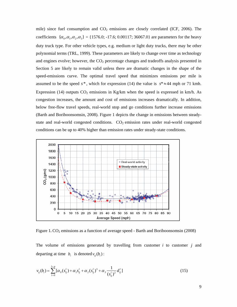
Expression (14) outputs CO2 emissions in Kg/km when the speed is expressed in km/h. As

congestion increases, the amount and cost of emissions increases dramatically. In addition,

below free-flow travel speeds, real-world stop and go conditions further increase emissions

(Barth and Boriboonsomsin, 2008). Figure 1 depicts the change in emissions between steady-

state and real-world congested conditions. CO2 emission rates under real-world congested

conditions can be up to 40% higher than emission rates under steady-state conditions.

Figure 1. CO2 emissions as a function of average speed - Barth and Boriboonsomsin (2008)

The volume of emissions generated by travelling from customer i to customer j and

departing at time ib is denoted ( )ij iv b :

( )ij iv b = 30 1 2 3 2

0

1[ ( ) ( ) ]( )

l pl l l lij ij ij ijl

l ij

s s s ds

α α α α=

=

+ + +∑ (15)

10

Expression (15) provides a simple yet good approximation for real-world CO2 emissions vs.

travel speed profiles. Acceleration impacts are not considered because detailed speed profiles

will be required; however, to account for the emission rate increases in stop-and-go traffic

conditions, the term 0 ( )lijsα could be adjusted.

Speed Constraints

Travel speeds are limited by speed limits or congestion. As indicated by constraint (16), a

vehicle traveling between two costumers ,i j cannot exceed the travel speed for that link in

period of time l .

l l lij ij ijs s s≤ ≤ (16)

In addition, travel speeds are also limited by road characteristics. To represent different road

characteristics between two customers ,i j the segment of distance ijd is partitioned into a set

of ( , )R i j segments that for the partial distance set:

1 2 ( , ){ , , ..., }R i jij ij ijr r r such that

' ( , )'

' 1

l R i jl

ij ijl

d r=

=

= ∑

Each segment 'lijr has an upper and lower speed bounds. Combining speed constraints due to

time of the day and road section we obtain the more general constraint expression (17) for

time of day l and section 'l between customers ,i j :

, ' , ' , 'l l l l l lij ij ijs s s≤ ≤ (17)

4. Portland Case Study

Considered a gateway to international sea and air freight transport, the city of Portland has

established itself both in name and trade as an important component of both international and

domestic freight movements. Its favorable geography to both international ocean and

domestic river freight via the Columbia River is also complimented by its connection to

Interstate-5 (I-5), providing good connectivity to southern California ports and international

freight traffic from Mexico and Canada (EDRG, 2007). Recent increases in regional

11

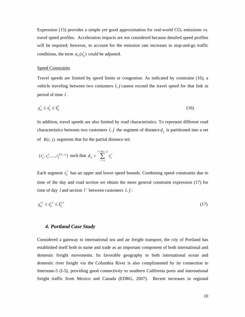
congestion, however, have hindered considerably freight operations and brought about a

substantial increase in delivery costs (Conrad and Figliozzi, 2010).

Figure 2. Depots and Customer Locations (base map sourced from Google maps1)

The I-5 freeway corridor provides the main north-south freight corridor and is used by most

carriers delivering in downtown Portland, regional through traffic, and many commuters.

Land use patterns are used to locate two carrier’s depots in warehousing/industrial areas that

are located in relatively central and suburban locations respectively. The I-5 freeway corridor,

even under congested conditions, provides the shortest distance and time path between the

urban and suburban depot and downtown Portland. Freeway, arterial, and local segments are

established for each path as required by expression (17).

1 Google Maps at http://maps.google.com

Central Depot

City Customers with hard time windows

Central Depot

Suburban Depot

12

Figure 2 also shows the relative location of downtown Portland, the I-5 corridor, the central

depot, and the suburban depot. Experimental results described in Section 5 utilize the central

and suburban depot locations shown in Figure 2 as well as an intermediate depot location (not

shown in shown in Figure 2) located between the central customers and the suburban depot.

The intermediate depot is located on I-5 at a distance that is approximately 1/3 of the distance

between the central customers and the suburban depot. The central, intermediate, and

suburban depots are located in areas with warehousing or related land uses or commercial

activities.

Travel Speed Data

Time-dependent travel speed data comes from 436 inductive loop detectors along interstate

freeways in the Portland metropolitan area. Traffic data is systematically archived in the

Portland Oregon Transportation Archived Listing (PORTAL). A complete description of this

data source is given by Bertini et al. (2005). The travel speeds used in this research are

calculated from 15 minute archived travel time data averaged over the year 2007 along the I-5

freeway corridor spanning from the Portland suburb of Wilsonville to Vancouver,

Washington. In addition, Portland State University had access to truck GPS location and time

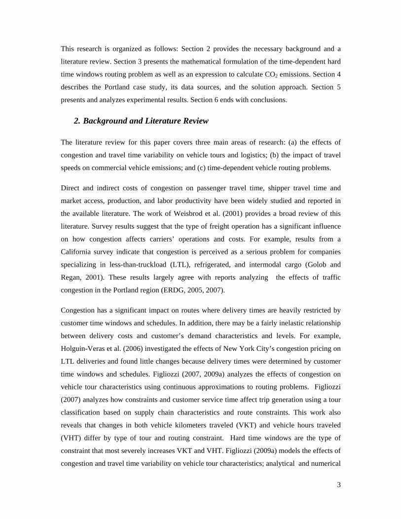
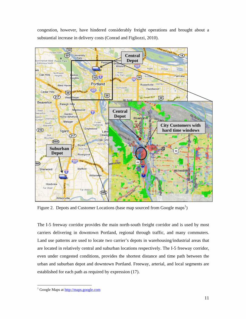
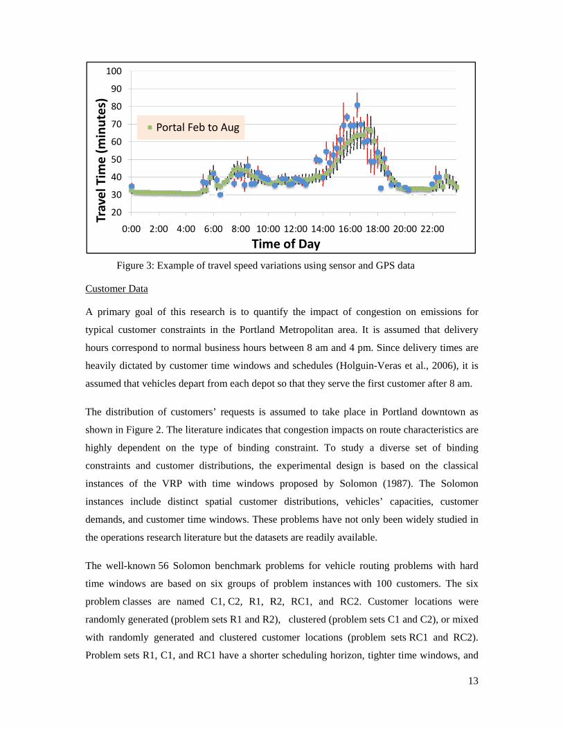
data that can be used to calculate travel speeds (Wheeler and Figliozzi, 2009). Figure 3

compares a typical week of average time-dependent travel time data using sensor data from

PORTAL and GPS base data for a section of Interstate 5; historical travel time speeds based

on sensor data are a good proxy for truck travel speeds.

Figure 3 also shows that free-flow travel speeds, around 60 miles per hour, take place at night

– mostly between 9 pm and 6 am. Some commercial vehicles travel at speeds as high as 70 or

75 miles per hour. This research assumes that travel speeds between 6 am and 9 pm are a

function of time of the day. The base scenario, uncongested travel times, assumes a constant

time dependent speed of 65 miles per hour in the freeways and 30 miles per hour in the

arterial network. Travel speed on arterials is based on speed limits during uncongested hours

and estimating congested travel times based on patterns observed in the Portland area (Wolfe

et al., 2007). The percentage of local street travel is relatively small and mostly limited to

connections between customers and freeways/arterials. Local speed is assumed to have a

constant value of 10 miles per hour.

Fi

Customer

A primar

typical cu

hours cor

heavily d

assumed

The distr

shown in

highly d

constrain

instances

instances

demands,

the opera

The well

time win

problem c

randomly

with rand

Problem

20

30

40

50

60

70

80

90

100

0

Travel Tim

e (m

inutes)

igure 3: Exa

r Data

ry goal of t

ustomer con

rrespond to n

dictated by c

that vehicles

ribution of c

n Figure 2. T

ependent on

nts and cust

s of the VR

s include d

, and custom

ations researc

l-known 56

ndows are b

classes are

y generated (

domly gene

sets R1, C1

0:00 2:00

Por

ample of trav

this research

nstraints in

normal busin

customer tim

s depart from

customers’ r

he literature

n the type

tomer distrib

RP with tim

distinct spat

mer time win

ch literature

Solomon be

ased on six

named C1

(problem set

erated and c

, and RC1 h

4:00 6:00

tal Feb to A

vel speed var

h is to quan

the Portland

ness hours b

me windows

m each depo

requests is a

e indicates th

of binding

butions, the

me windows

ial custome

ndows. Thes

but the data

enchmark pr

x groups of

, C2, R1, R

ts R1 and R2

clustered cu

have a shorte

0 8:00 10:0

Tim

Aug

riations usin

ntify the imp

d Metropolit

between 8 am

and schedu

t so that they

assumed to

hat congestio

constraint.

experiment

s proposed

er distributi

se problems

asets are read

roblems for

problem ins

R2, RC1, a

2), clustere

ustomer loca

er schedulin

00 12:00 14

me of Day

g sensor and

pact of con

tan area. It

m and 4 pm

les (Holguin

y serve the f

take place i

on impacts o

To study a

tal design i

by Solomo

ions, vehicl

have not on

dily available

vehicle rou

stances with

and RC2. C

d (problem s

ations (probl

ng horizon, t

:00 16:00 1

d GPS data

ngestion on

is assumed

m. Since deliv

n-Veras et a

first custome

in Portland

on route char

a diverse se

is based on

on (1987). T

es’ capaciti

nly been wid

e.

uting proble

h 100 custom

Customer lo

sets C1 and

lem sets RC

tighter time w

8:00 20:00

1

emissions f

that deliver

very times a

al., 2006), it

er after 8 am

downtown

racteristics a

et of bindin

the classic

The Solomo

ies, custom

dely studied

ms with har

mers. The s

ocations we

C2), or mixe

C1 and RC2

windows, an

22:00

13

for

ry

are

is

m.

as

are

ng

cal

on

mer

in

rd

six

ere

ed

2).

nd

14

fewer customers per route than problem sets R2, C2, and RC2 respectively. Demand

constraints are binding for C1 and C2 problems whereas time-window constraints are binding

for R1, R2, RC1, and RC2 problems. In this research the Solomon customer time windows

are made proportional to the assumed normal business hours between 8 am and 4 pm so the

original demand and time window constraints are maintained. Customer locations have been

scaled to fit Portland downtown area but the relative spatial distribution among customers has

been preserved.

Solution Algorithm

The time-dependent vehicle routing problems are solved using the route construction and

improvement algorithm described in detail in Figliozzi (2009c). This approach, also denoted

IRCI for Iterated Route Construction and Improvement has also been successfully applied to

VRP problems with soft time windows (Figliozzi, 2009b). As in previous research efforts

with a exploratory and policy motivation (Quak and de Koster, 2007), the focus of this

research is not on finding optimal routes for simpler problems (i.e. constant travel times

problems) but on approximating carriers’ route planning as well as possible and capturing the

trade-off between congestion, depot locations, customer characteristics, and CO2 emissions in

the case study area.

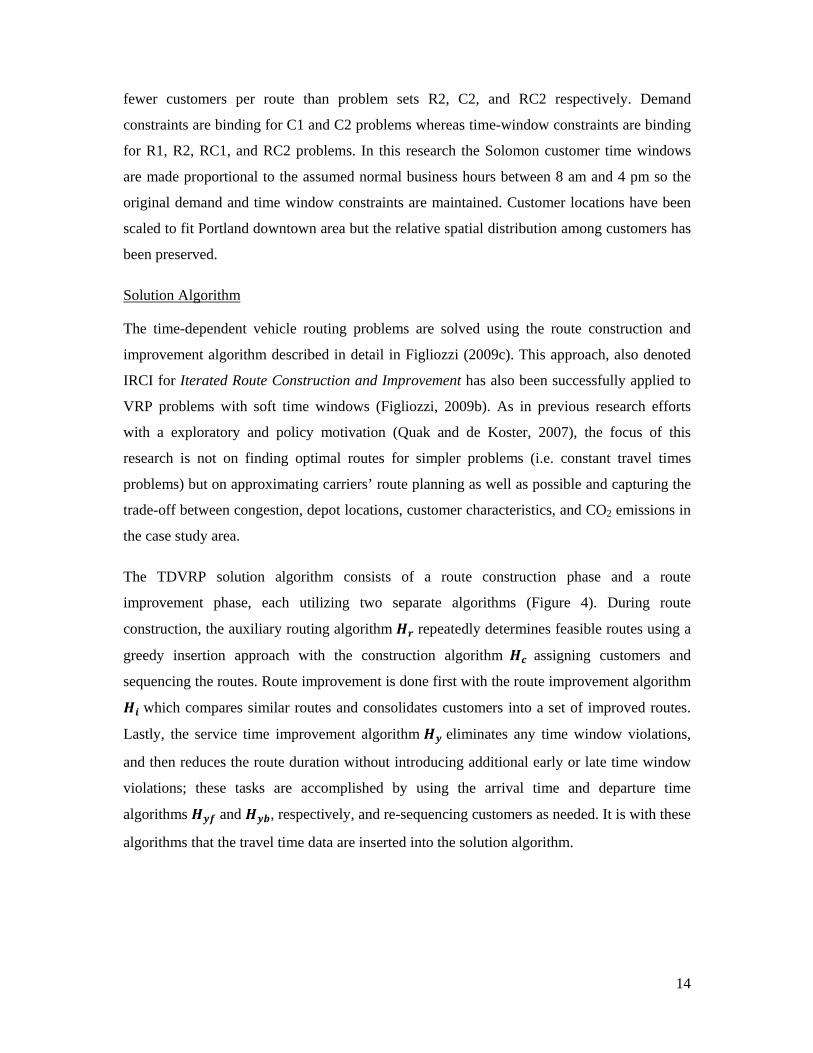
The TDVRP solution algorithm consists of a route construction phase and a route

improvement phase, each utilizing two separate algorithms (Figure 4). During route

construction, the auxiliary routing algorithm repeatedly determines feasible routes using a

greedy insertion approach with the construction algorithm assigning customers and

sequencing the routes. Route improvement is done first with the route improvement algorithm

which compares similar routes and consolidates customers into a set of improved routes.

Lastly, the service time improvement algorithm eliminates any time window violations,

and then reduces the route duration without introducing additional early or late time window

violations; these tasks are accomplished by using the arrival time and departure time

algorithms and , respectively, and re-sequencing customers as needed. It is with these

algorithms that the travel time data are inserted into the solution algorithm.

15

Figure 4: Solution method of the iterative route construction and improvement (IRCI)algorithm.

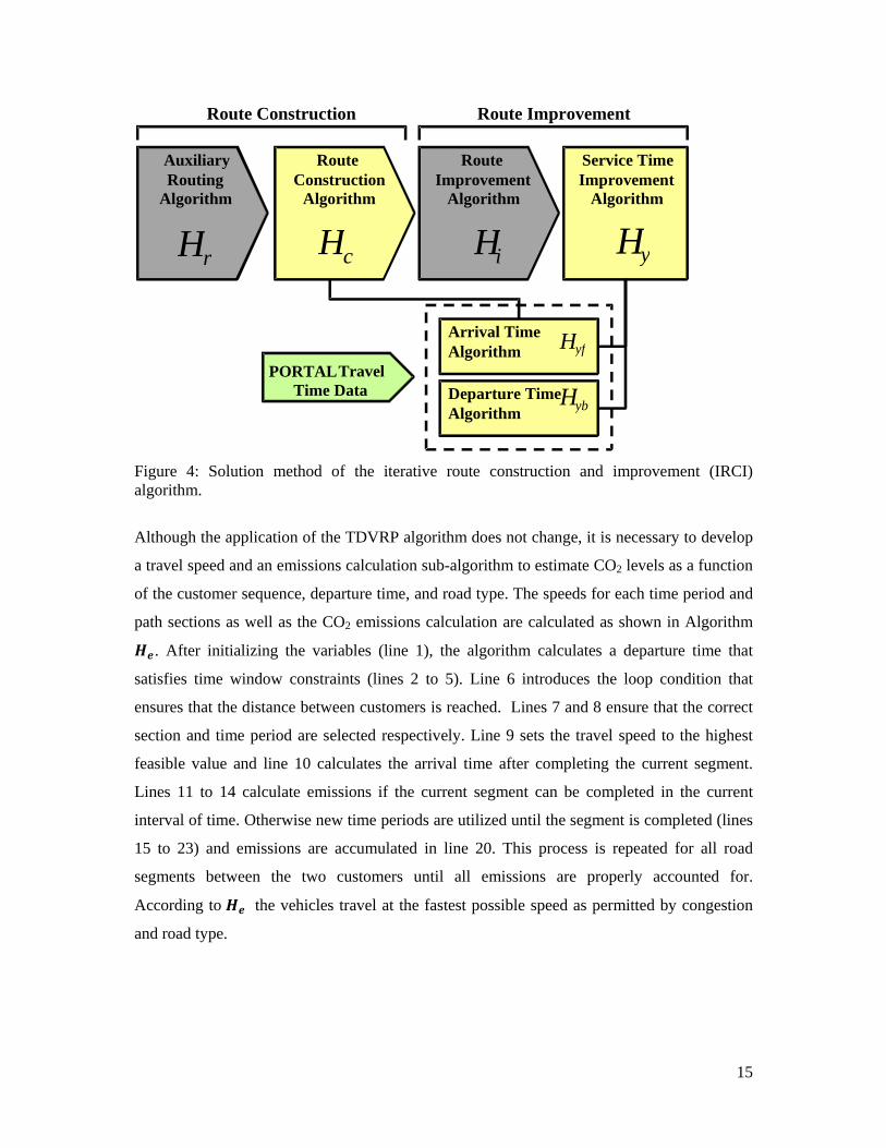
Although the application of the TDVRP algorithm does not change, it is necessary to develop

a travel speed and an emissions calculation sub-algorithm to estimate CO2 levels as a function

of the customer sequence, departure time, and road type. The speeds for each time period and

path sections as well as the CO2 emissions calculation are calculated as shown in Algorithm

. After initializing the variables (line 1), the algorithm calculates a departure time that

satisfies time window constraints (lines 2 to 5). Line 6 introduces the loop condition that

ensures that the distance between customers is reached. Lines 7 and 8 ensure that the correct

section and time period are selected respectively. Line 9 sets the travel speed to the highest

feasible value and line 10 calculates the arrival time after completing the current segment.

Lines 11 to 14 calculate emissions if the current segment can be completed in the current

interval of time. Otherwise new time periods are utilized until the segment is completed (lines

15 to 23) and emissions are accumulated in line 20. This process is repeated for all road

segments between the two customers until all emissions are properly accounted for.

According to the vehicles travel at the fastest possible speed as permitted by congestion

and road type.

AuxiliaryRouting

Algorithm

rH

Route Construction

Algorithm

c H

Route Improvement

Algorithm

iH

Service Time Improvement

Algorithm

y H

Route Construction Route Improvement

Arrival TimeAlgorithm

Departure Time Algorithm

PORTALTravel Time Data

yfH

ybH

16

Algorithm Data: T and S : time intervals and speeds

, , ,i j i iv v a b : two customers ,i jv v served in this order in route k , ia is the current arrival

time at customer i and ib the proposed departure time START

initialize 0,D ← 0,t ← ( ) 0ij iv b ← 1

if ib < max( , )i i ie a g+ then 2

max( , ) ,i i i i ib e a g t b← + ← 3

else it b← 4 end if 5 while ijD d≤ do 6

find min( ')k such that'

'

1

kk

ijD r≤∑ 7

find k such that k kt t t≤ ≤ 8 , 'k k

ijs s← 9 '

' /kk ija t r s← + 10

if 'k ka t< then 11

( ) ( )ij i ij iv b v b← + formula (15) with speed 'kks , distance 'kijr 12

' ', max( , ),k kij i k ijd r t b t D D r← ← ← + 13

end if 14 while 'k ka t> do 15

'( ) kkkd d t t s← − − 16

'( ) kkkD D t t s← + − 17 1, '

1, ', k kk k ijkt t s s ++← ← 18

' 1, '/k k ka t d s +← + 19

( ) ( )ij i ij iv b v b← + formula (15) with speed 1, ' ,k ks + distance 20

' 1, '1(min( , ) )k k kka t t s ++ − 21

1k k← + 22 end while 23

end while24 END Output:

'ka , arrival time at customer j

( )ij iv b = CO2 emissions between customers ,i j for a departure time ib

17

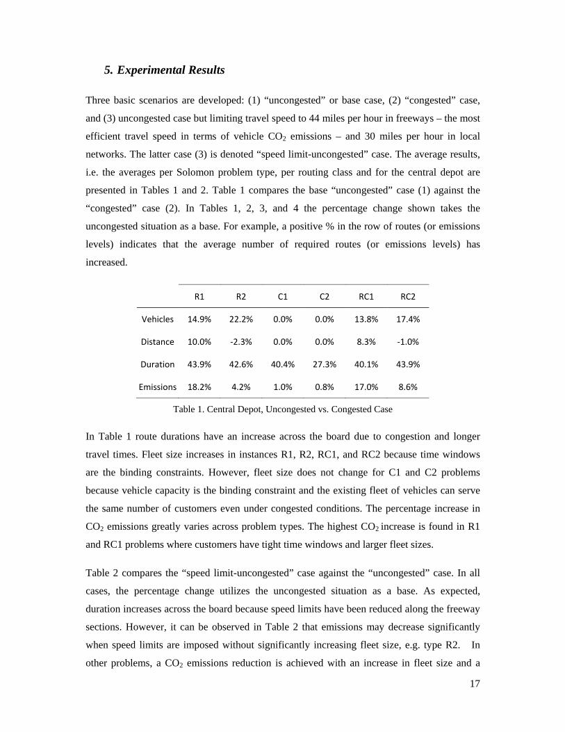
5. Experimental Results

Three basic scenarios are developed: (1) “uncongested” or base case, (2) “congested” case,

and (3) uncongested case but limiting travel speed to 44 miles per hour in freeways – the most

efficient travel speed in terms of vehicle CO2 emissions – and 30 miles per hour in local

networks. The latter case (3) is denoted “speed limit-uncongested” case. The average results,

i.e. the averages per Solomon problem type, per routing class and for the central depot are

presented in Tables 1 and 2. Table 1 compares the base “uncongested” case (1) against the

“congested” case (2). In Tables 1, 2, 3, and 4 the percentage change shown takes the

uncongested situation as a base. For example, a positive % in the row of routes (or emissions

levels) indicates that the average number of required routes (or emissions levels) has

increased.

R1  R2  C1  C2  RC1  RC2 

Vehicles  14.9%  22.2%  0.0%  0.0%  13.8%  17.4% 

Distance  10.0%  ‐2.3%  0.0%  0.0%  8.3%  ‐1.0% 

Duration  43.9%  42.6%  40.4%  27.3%  40.1%  43.9% 

Emissions  18.2%  4.2%  1.0%  0.8%  17.0%  8.6% 

Table 1. Central Depot, Uncongested vs. Congested Case

In Table 1 route durations have an increase across the board due to congestion and longer

travel times. Fleet size increases in instances R1, R2, RC1, and RC2 because time windows

are the binding constraints. However, fleet size does not change for C1 and C2 problems

because vehicle capacity is the binding constraint and the existing fleet of vehicles can serve

the same number of customers even under congested conditions. The percentage increase in

CO2 emissions greatly varies across problem types. The highest CO2 increase is found in R1

and RC1 problems where customers have tight time windows and larger fleet sizes.

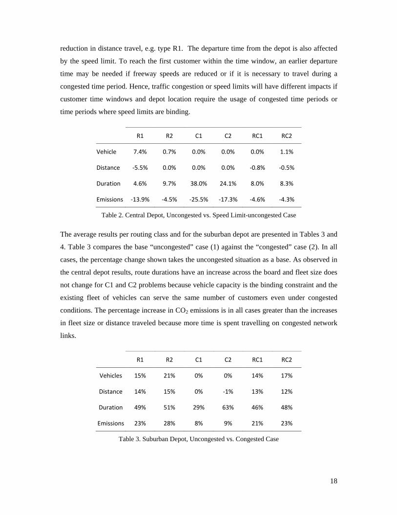
Table 2 compares the “speed limit-uncongested” case against the “uncongested” case. In all

cases, the percentage change utilizes the uncongested situation as a base. As expected,

duration increases across the board because speed limits have been reduced along the freeway

sections. However, it can be observed in Table 2 that emissions may decrease significantly

when speed limits are imposed without significantly increasing fleet size, e.g. type R2. In

other problems, a CO2 emissions reduction is achieved with an increase in fleet size and a

18

reduction in distance travel, e.g. type R1. The departure time from the depot is also affected

by the speed limit. To reach the first customer within the time window, an earlier departure

time may be needed if freeway speeds are reduced or if it is necessary to travel during a

congested time period. Hence, traffic congestion or speed limits will have different impacts if

customer time windows and depot location require the usage of congested time periods or

time periods where speed limits are binding.

   R1  R2  C1  C2  RC1  RC2 

Vehicle  7.4%  0.7%  0.0%  0.0%  0.0%  1.1% 

Distance  ‐5.5%  0.0%  0.0%  0.0%  ‐0.8%  ‐0.5% 

Duration  4.6%  9.7%  38.0%  24.1%  8.0%  8.3% 

Emissions  ‐13.9%  ‐4.5%  ‐25.5%  ‐17.3%  ‐4.6%  ‐4.3% 

Table 2. Central Depot, Uncongested vs. Speed Limit-uncongested Case

The average results per routing class and for the suburban depot are presented in Tables 3 and

4. Table 3 compares the base “uncongested” case (1) against the “congested” case (2). In all

cases, the percentage change shown takes the uncongested situation as a base. As observed in

the central depot results, route durations have an increase across the board and fleet size does

not change for C1 and C2 problems because vehicle capacity is the binding constraint and the

existing fleet of vehicles can serve the same number of customers even under congested

conditions. The percentage increase in CO2 emissions is in all cases greater than the increases

in fleet size or distance traveled because more time is spent travelling on congested network

links.

   R1  R2  C1  C2  RC1  RC2 

Vehicles  15%  21%  0%  0%  14%  17% 

Distance  14%  15%  0%  ‐1%  13%  12% 

Duration  49%  51%  29%  63%  46%  48% 

Emissions  23%  28%  8%  9%  21%  23% 

Table 3. Suburban Depot, Uncongested vs. Congested Case

19

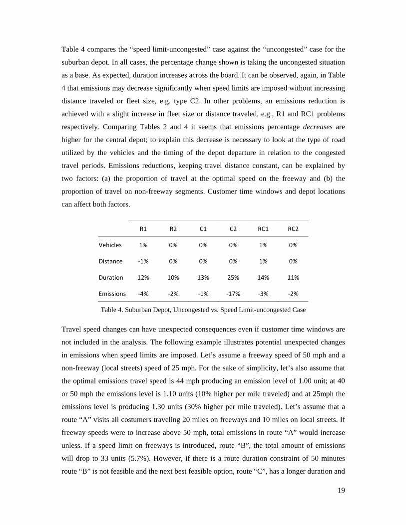
Table 4 compares the “speed limit-uncongested” case against the “uncongested” case for the

suburban depot. In all cases, the percentage change shown is taking the uncongested situation

as a base. As expected, duration increases across the board. It can be observed, again, in Table

4 that emissions may decrease significantly when speed limits are imposed without increasing

distance traveled or fleet size, e.g. type C2. In other problems, an emissions reduction is

achieved with a slight increase in fleet size or distance traveled, e.g., R1 and RC1 problems

respectively. Comparing Tables 2 and 4 it seems that emissions percentage decreases are

higher for the central depot; to explain this decrease is necessary to look at the type of road

utilized by the vehicles and the timing of the depot departure in relation to the congested

travel periods. Emissions reductions, keeping travel distance constant, can be explained by

two factors: (a) the proportion of travel at the optimal speed on the freeway and (b) the

proportion of travel on non-freeway segments. Customer time windows and depot locations

can affect both factors.

R1  R2  C1  C2  RC1  RC2 

Vehicles  1%  0%  0%  0%  1%  0% 

Distance  ‐1%  0%  0%  0%  1%  0% 

Duration  12%  10%  13%  25%  14%  11% 

Emissions  ‐4%  ‐2%  ‐1%  ‐17%  ‐3%  ‐2% 

Table 4. Suburban Depot, Uncongested vs. Speed Limit-uncongested Case

Travel speed changes can have unexpected consequences even if customer time windows are

not included in the analysis. The following example illustrates potential unexpected changes

in emissions when speed limits are imposed. Let’s assume a freeway speed of 50 mph and a

non-freeway (local streets) speed of 25 mph. For the sake of simplicity, let’s also assume that

the optimal emissions travel speed is 44 mph producing an emission level of 1.00 unit; at 40

or 50 mph the emissions level is 1.10 units (10% higher per mile traveled) and at 25mph the

emissions level is producing 1.30 units (30% higher per mile traveled). Let’s assume that a

route “A” visits all costumers traveling 20 miles on freeways and 10 miles on local streets. If

freeway speeds were to increase above 50 mph, total emissions in route “A” would increase

unless. If a speed limit on freeways is introduced, route “B”, the total amount of emissions

will drop to 33 units (5.7%). However, if there is a route duration constraint of 50 minutes

route “B” is not feasible and the next best feasible option, route “C”, has a longer duration and

20

distance traveled than route “A”. However, total emissions are reduced to 33.2 units (5.3%)

because the proportion of freeway travel has increased. Furthermore, if the objective function

is to reduce fleet and distance, a suboptimal choice from the emissions perspective will be

made if route “D” (with longer travel distance) but less emissions is not chosen. If the

reduction of freeway speed is more than it is required (congestion), the results are even worse

than in the initial starting point (compare route “E” vs. route “A”). Hence, policies that aim to

reduce CO2 emission levels by reducing speed limits will be more successful if (a) freeway

travel speeds are at the optimum emissions speed level, (b) the imposition of a speed limit

does not increase the proportion of distance traveled in local roads, and (c) the overall

distance traveled does not increase. When time windows are present, the analysis is more

difficult because the departure time from the depot is also constrained by the speed limit or

the timing of the congested period (to reach the first customer within the time window, an

earlier departure time may be needed if freeway speeds are reduced or if it is necessary to

travel during a congested time period).

Route  Speed Emission Factors  Distance   Total 

Freeway  Local  Freeway  Local  Freeway  Local  Distance  Duration  Emissions 

A  50.0  25.0  1.1  1.3  20.0  10.0  30.0  48.0  35.0 

B  44.0  25.0  1.0  1.3  20.0  10.0  30.0  51.3  33.0 

C  44.0  25.0  1.0  1.3  26.0  5.5  31.5  48.7  33.2 

D  44.0  25.0  1.0  1.3  27.1  4.5  31.6  47.8  33.0 

 E  40.0  25.0  1.1  1.3  28.5  3.0  31.5  50.0  35.3 

Table 5. Route comparisons when speed and duration constraints are introduced

Important emission reductions can be obtained by optimizing travel speeds. However, it

should be clear that depot location has a significant role on total level of emissions. To better

illustrate this point a new depot, the intermediate depot, is added approximately 1/3 of the

way between the central area and the suburban depot. To simplify comparisons, there are no

changes in vehicle fleet size and local distance in Tables 6 and 7 because vehicles in the

intermediate and suburban depots are allowed to depart earlier and return later. In addition,

depots time windows are relaxed so that the same routes are followed. In both Tables 6 and 7,

the percentage changes utilize the central depot case (uncongested and congested respectively)

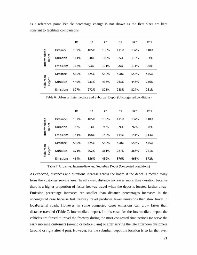
21

as a reference point Vehicle percentage change is not shown as the fleet sizes are kept

constant to facilitate comparisons.

  R1  R2  C1  C2  RC1  RC2 Interm

ediate 

Dep

ot 

Distance  137%  105%  136%  111%  137%  110% 

Duration  111%  58%  108%  65%  110%  63% 

Emissions  112%  93%  111%  96%  111%  96% 

Subu

rban

  Dep

ot 

Distance  555%  425%  550%  450%  554%  445% 

Duration  449%  233%  436%  263%  446%  256% 

Emissions  327%  272%  325%  283%  327%  281% 

Table 6. Urban vs. Intermediate and Suburban Depot (Uncongested conditions)

  R1  R2  C1  C2  RC1  RC2 

Interm

ediate 

Dep

ot 

Distance  137%  105%  136%  111%  137%  110% 

Duration  98%  53%  95%  59%  97%  58% 

Emissions  141%  108%  140%  114%  141%  113% 

Subu

rban

   Dep

ot 

Distance  555%  425%  550%  450%  554%  445% 

Duration  371%  202%  361%  227%  368%  221% 

Emissions  464%  356%  459%  376%  463%  372% 

Table 7. Urban vs. Intermediate and Suburban Depot (Congested conditions)

As expected, distances and durations increase across the board if the depot is moved away

from the customer service area. In all cases, distance increases more than duration because

there is a higher proportion of faster freeway travel when the depot is located farther away.

Emission percentage increases are smaller than distance percentages increases in the

uncongested case because fast freeway travel produces fewer emissions than slow travel in

local/arterial roads. However, in some congested cases emissions can grow faster than

distance traveled (Table 7, intermediate depot). In this case, for the intermediate depot, the

vehicles are forced to travel the freeway during the most congested time periods (to serve the

early morning customers (around or before 8 am) or after serving the late afternoon customers

(around or right after 4 pm). However, for the suburban depot the location is so far that even

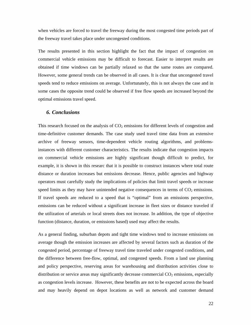
22

when vehicles are forced to travel the freeway during the most congested time periods part of

the freeway travel takes place under uncongested conditions.

The results presented in this section highlight the fact that the impact of congestion on

commercial vehicle emissions may be difficult to forecast. Easier to interpret results are

obtained if time windows can be partially relaxed so that the same routes are compared.

However, some general trends can be observed in all cases. It is clear that uncongested travel

speeds tend to reduce emissions on average. Unfortunately, this is not always the case and in

some cases the opposite trend could be observed if free flow speeds are increased beyond the

optimal emissions travel speed.

6. Conclusions

This research focused on the analysis of CO2 emissions for different levels of congestion and

time-definitive customer demands. The case study used travel time data from an extensive

archive of freeway sensors, time-dependent vehicle routing algorithms, and problems-

instances with different customer characteristics. The results indicate that congestion impacts

on commercial vehicle emissions are highly significant though difficult to predict, for

example, it is shown in this researc that it is possible to construct instances where total route

distance or duration increases but emissions decrease. Hence, public agencies and highway

operators must carefully study the implications of policies that limit travel speeds or increase

speed limits as they may have unintended negative consequences in terms of CO2 emissions.

If travel speeds are reduced to a speed that is “optimal” from an emissions perspective,

emissions can be reduced without a significant increase in fleet sizes or distance traveled if

the utilization of arterials or local streets does not increase. In addition, the type of objective

function (distance, duration, or emissions based) used may affect the results.

As a general finding, suburban depots and tight time windows tend to increase emissions on

average though the emission increases are affected by several factors such as duration of the

congested period, percentage of freeway travel time traveled under congested conditions, and

the difference between free-flow, optimal, and congested speeds. From a land use planning

and policy perspective, reserving areas for warehousing and distribution activities close to

distribution or service areas may significantly decrease commercial CO2 emissions, especially

as congestion levels increase. However, these benefits are not to be expected across the board

and may heavily depend on depot locations as well as network and customer demand

23

characteristics. Further research is needed to explore alternative policies to minimize

emissions in congested areas without increasing logistics costs or decreasing customer service

levels.

24

Acknowledgements

The author gratefully acknowledges the Oregon Transportation, Research and Education

Consortium (OTREC) and Portland State University Research Administration for sponsoring

this research. The author also thanks graduate students Alex Bigazzi, Ryan Conrad,

Myeonwoo Lim, and Nikki Wheeler for editing this paper and assisting with congesting data

collection and graphs.

25

References

AHN, B. H. & SHIN, J. Y. (1991) Vehicle-routing with time windows and time-varying congestion. Journal of the Operational Research Society, 42(5), 393-400.

BARTH, M. & BORIBOONSOMSIN, K. (2008) Real-World Carbon Dioxide Impacts of Traffic Congestion. Transportation Research Record 2058, 163-171.

BAUMGARTNER, M., LÉONARDI, J. & KRUSCH, O. (2008) Improving computerized routing and scheduling and vehicle telematics: A qualitative survey. Transportation Research Part D, 13(6), 377-382.

BERTINI, R. L., HANSEN, S., MATTHEWS, S., RODRIGUEZ, A. & DELCAMBRE, A. (2005) PORTAL: Implementing a New Generation Archive Data User Service in Portland, Oregon. 12th World Congress on ITS, 1976(November).

CONRAD, R. & FIGLIOZZI, M. A. (2010) Algorithms to Quantify the Impacts of Congestion on Time-Dependent Real-World Urban Freight Distribution Networks. Proceedings of the 89th Transportation Research Board Annual Meeting CD rom - Washington DC. USA, web.cecs.pdx.edu/~maf/publications.html.

CORDEAU, J. F., LAPORTE, G., SAVELSBERGH, M. & VIGO, D. (2006) Vehicle Routing. IN BARNHART, C. & LAPORTE, G. (Eds.) Transportation, Handbooks in Operations Research and Management Science. Amsterdam, North-Holland.

CRAINIC, T. G., RICCIARDI, N. & STORCHI, G. (2004) Advanced freight transportation systems for congested urban areas. Transportation Research Part C: Emerging Technologies, 12(2), 119.

CRAINIC, T. G., RICCIARDI, N. & STORCHI, G. (2009) Models for Evaluating and Planning City Logistics Systems. Transportation Science, 43(4), 432-454.

DESROCHERS, M., LENSTRA, J. K., SAVELSBERGH, M. W. P. & SOUMIS, F. (1988) Vehicle routing with time windows: optimization and approximation. Vehicle Routing: Methods and Studies, 16(65-84.

DONATI, A. V., MONTEMANNI, R., CASAGRANDE, N., RIZZOLI, A. E. & GAMBARDELLA, L. M. (2008) Time dependent vehicle routing problem with a multi ant colony system. European Journal of Operational Research, 185(3), 1174-1191.

EDRG (2007) The Cost of Highway Limitations and Traffic Delay to Oregon's Economy. Portland, OR.

ERDG (2005) The Cost of Congestion to the Economy of the Portland Region, Economic Research Development Group, December 2005. Boston, MA, accessed June 2008, http://www.portofportland.com/Trade_Trans_Studies.aspx.

ERDG (2007) The Cost of Highway Limitations and Traffic Delay to Oregon’s Economy, Economic Research Development Group, March 2007. Boston, MA, accessed October 2008, http://www.portofportland.com/Trade_Trans_Studies_CostHwy_Lmtns.pdf.

FIGLIOZZI, M. A. (2007) Analysis of the efficiency of urban commercial vehicle tours: Data collection, methodology, and policy implications. Transportation Research Part B, 41(9), 1014-1032.

FIGLIOZZI, M. A. (2009a) The Impact of Congestion on Commercial Vehicle Tours and Costs. Transportation Research part E: Logistics and Transportation.

FIGLIOZZI, M. A. (2009b) An Iterative Route Construction and Improvement Algorithm for the Vehicle Routing Problem with Soft-time Windows. Transportation Research Part C: New Technologies.

FIGLIOZZI, M. A. (2009c) A Route Improvement Algorithm for the Vehicle Routing Problem with Time Dependent Travel Times. Proceeding of the 88th Transportation

26

Research Board Annual Meeting CD rom. Washington, DC, January 2009, also available at http://web.cecs.pdx.edu/~maf/publications.html.

FIGLIOZZI, M. A. (2010) Emissions Minimization Vehicle Routing Problem. Forthcoming Transportation Research Record 2010.

FLEISCHMANN, B., GIETZ, M. & GNUTZMANN, S. (2004) Time-varying travel times in vehicle routing. Transportation Science, 38(2), 160-173.

FREY, H., ROUPHAIL, N. & ZHAI, H. (2008) Link-Based Emission Factors for Heavy-Duty Diesel Trucks Based on Real-World Data. Transportation Research Record, 2058(23-332.

GOLOB, T. F. & REGAN, A. C. (2001) Impacts of highway congestion on freight operations: perceptions of trucking industry managers. Transportation Research Part A: Policy and Practice, 35(7), 577-599.

HAGHANI, A. & JUNG, S. (2005) A dynamic vehicle routing problem with time-dependent travel times. Computers & Operations Research, 32(11), 2959-2986.

HOLGUIN-VERAS, J., WANG, Q., XU, N., OZBAY, K., CETIN, M. & POLIMENI, J. (2006) The impacts of time of day pricing on the behavior of freight carriers in a congested urban area: Implications to road pricing. Transportation Research Part A-Policy And Practice, 40(9), 744-766.

ICF (2006) Assessment of Greenhouse Gas Analysis Techniques for Transportation Projects, NCHRP Project 25-25 Task 17, ICF Consulting. Fairfax, VA.

ICHOUA, S., GENDREAU, M. & POTVIN, J. Y. (2003) Vehicle dispatching with time-dependent travel times. European Journal Of Operational Research, 144(2), 379-396.

JUNG, S. & HAGHANI, A. (2001) Genetic Algorithm for the Time-Dependent Vehicle Routing Problem. Transportation Research Record, 1771(-1), 164-171.

LÉONARDI, J. & BAUMGARTNER, M. (2004) CO2 efficiency in road freight transportation: Status quo, measures and potential. Transportation Research Part D, 9(6), 451-464.

MALANDRAKI, C. (1989) Time dependent vehicle routing problems: Formulations, solution algorithms and computational experiments. Evanston, Illinois., Ph.D. Dissertation, Northwestern University.

MALANDRAKI, C. & DASKIN, M. S. (1992) Time-Dependent Vehicle-Routing Problems - Formulations, Properties And Heuristic Algorithms. Transportation Science, 26(3), 185-200.

OECD (2003) Delivering the Goods 21st Century Challenges to Urban Goods Transport, OECD Organisation for Economic Co-operation and Development.

PALMER, A. (2008) The development of an integrated routing and carbon dioxide emissions model for goods vehicles. PhD Thesis Cranfield University November 2007.

QUAK, H. J. & DE KOSTER, M. B. M. (2007) Exploring retailers' sensitivity to local sustainability policies. Journal of Operations Management, 25(6), 1103.

QUAK, H. J. H. & DE KOSTER, M. (2009) Delivering Goods in Urban Areas: How to Deal with Urban Policy Restrictions and the Environment. Transportation Science, 43(2), 211-227.

ROPKINS, K., BEEBE, J., LI, H., DAHAM, B., TATE, J., BELL, M. & ANDREWS, G. (2009) Real-World Vehicle Exhaust Emissions Monitoring: Review and Critical Discussion. Critical Reviews in Environmental Science and Technology, 39(2), 79-152.

SBIHI, A. & EGLESE, R. W. (2007) Combinatorial optimization and Green Logistics. 4OR: A Quarterly Journal of Operations Research, 5(2), 99-116.

SOLOMON, M. M. (1987) Algorithms For The Vehicle-Routing And Scheduling Problems With Time Window Constraints. Operations Research, 35(2), 254-265.

27

TANIGUCHI, E., THOMPSON, R. G. & YAMADA, T. (2003) Predicting the effects of city logistics schemes. Transport Reviews, 23(4), 489-515.

TRL (1999) Methodology for calculating transport emissions and energy consumption. Transport Research Laboratory, Crowthorne, United Kingdom. Edited by A J Hickman, Project Report SE/491/98, Deliverable 22 for the project MEET (Methodologies for estimating air pollutant emissions from transport).

WEISBROD, G., DONALD, V. & TREYZ, G. (2001) Economic Implications of Congestion. NCHRP Report #463. Washington, DC, National Cooperative Highway Research Program, Transportation Research Board.

WHEELER, N. & FIGLIOZZI, M. A. (2009) Analysis of the Impacts of Congestion on Freight Movements in the Portland Metropolitan Area using GPS data. Proceedings 3nd Annual National Urban Freight Conference, Long Beach, CA. October 2009.

WOENSEL, T. V., CRETEN, R. & VANDAELE, N. (2001) Managing the environmental externalities of traffic logistics: The issue of emissions. Production and Operations Management, 10(2), 207-223.

WOLFE, M., MONSERE, C., KOONCE, P. & BERTINI, R. L. (2007) Improving Arterial Performance Measurement Using Traffic Signal System Data. Intelligent Transportation Systems Conference, 2007. ITSC 2007. IEEE, 113-118.