Marine Highway System – A Multimodal Short Sea Freight Shipping System

Marine Highway System (MHS)

(A Multimodal Short Sea Freight Shipping System)

Final Report

Prepared by:

Surface Congestion Reduction Analysis & Modeling Team

(SCRAM)

Karen Davis

Greg Haubner

James Hingst

Bill Judge

Chris Zalewski

George Mason University

Fairfax, VA

OR 680 Spring 2010

Date: May 7, 2010

i

Contents

1 Introduction ............................................................................................................................ 1

1.1 Background ........................................................................................................................ 1

1.2 Problem Statement and Scope ........................................................................................... 2

1.3 Customer and Stakeholders................................................................................................ 2

1.4 Surface Congestion Reduction Analysis & Modeling Team (SCRAM) ........................... 3

1.4.1 Karen Davis ................................................................................................................... 3

1.4.2 Greg Haubner ................................................................................................................. 3

1.4.3 James Hingst .................................................................................................................. 3

1.4.4 Bill Judge ....................................................................................................................... 4

1.4.5 Christopher Zalewski ..................................................................................................... 4

2 Technical Approach ............................................................................................................... 5

2.1 Problem Formulation and Analysis ................................................................................... 5

2.1.1 Problem Statement ......................................................................................................... 5

2.1.2 Assumptions and Limitations ........................................................................................ 5

2.2 Requirements Definition .................................................................................................... 7

2.3 Methodology ..................................................................................................................... 7

2.3.1 Project Design and Development................................................................................... 7

3 Results .................................................................................................................................. 17

3.1 Decision Analysis Tool Deliverables and Results ........................................................... 17

3.2 Simulation Deliverables and Results ............................................................................... 19

4 Discussion ............................................................................................................................ 22

5 Conclusions.......................................................................................................................... 24

5.1 Observations ................................................................................................................... 24

5.2 Follow on work............................................................................................................... 24

Appendix A. References ............................................................................................................... 27

Appendix B. Project Management Metrics ................................................................................... 28

Appendix C. Data Analysis Tool .................................................................................................. 30

Appendix D. Simulation ............................................................................................................... 38

ii

List of Figures

Figure 1. First Route Option between Richmond, VA and Norfolk, VA ..................................... 10

Figure 2. Second Route Option between Richmond, VA and Norfolk, VA ................................. 10

Figure 3. Third Route Option between Richmond, VA and Norfolk, VA .................................... 11

Figure 4. Marine Highway Simulation Flow Diagram ................................................................. 14

Figure 5. Surface Highway Simulation Flow Diagram ................................................................ 15

Figure 6. Cost per TEU versus MODA Metric ............................................................................. 17

Figure 7. Cost per TEU versus MODA Metric (24 hour gate operations and 2 cranes) .............. 18

Figure 8. Arena Surface Transportation Simulation ..................................................................... 38

Figure 9. Arena Port of Richmond Simulation ............................................................................. 41

Figure 10. Arena Port of Virginia Simulation .............................................................................. 42

iii

List of Tables

Table 1. Swing Weight Calculations ............................................................................................ 12

Table 2. Scenario Ship Type Summary ........................................................................................ 13

Table 3. Raw Metrics Used to Derive MODA Metrics ................................................................ 17

Table 4. Raw Metrics Used to Derive MODA Metrics (24 hour gate operations and 2 cranes) .. 18

Table 5. Travel time statistics for three routes .............................................................................. 39

Table 6: Normal and Unlimited Gate Hours Results .................................................................... 43

1

1 Introduction

1.1 Background With an ever increasing emphasis on efficiency, the motivation to explore innovative ways to improve the transportation of goods is also increasing. Companies and individuals are interested in not only optimizing cost and time but more recently, the carbon footprint of producing the various goods that fuel daily life. Regardless of the origination of goods (international or domestic production and manufacturing), there is a significant requirement for highway travel for interim and final destination delivery. Combining this demand with everyday commuting demands is one of the major contributing factors to growing roadway congestion. According to the "National Strategy to Reduce Congestion on America’s Transportation Network," Department of Transportation (May 2007),"...congestion is costing America an estimated $200 billion a year."1 Nearly 98 percent of all domestic freight, including through ports, moves on the United States’ highways and railroads.2 The Federal Highway Administration study entitled, “Estimated Cost of Freight Involved in Highway Bottlenecks – Final Report,” indicates that, on average, there are currently 10,500 trucks per day per mile on the Interstate Highway System. But by 2035, that volume is expected to double to 22,700 trucks, with the most heavily used portions of the system seeing upwards of 50,000 trucks per day.3 Urban communities will feel the greatest impact from the traffic volume increases. According to the Department of Transportation (DOT), trucks account for almost 40 percent of the time Americans spend stuck in traffic in the 50 most congested urban areas. Until recently, additional capacity demands were met by adding more highway lanes. But this is no longer a realistic option. Recent reports indicate that between highways and railroads more than $300 billion is needed to meet this future capacity demand. In addition, in 2007 more than 60 percent of federal highway funding went toward maintenance of existing roadways, leaving little for new development to help increase capacity.4 With the economic climate, the steady increase in population (and therefore demand), and the growing concern about climate change, the exploration of alternative methods for goods transport has become a priority. In addition to the growing research in alternative fuels and “just-in-time” delivery planning methodologies, freight movement options for trains and ships could provide viable solutions. According to the Marine Administration (MARAD) website, the Department of Transportation published an interim final rule on Oct. 9, 2008, establishing a framework to provide federal support to expand the use of America's Marine Highway. The four primary components of the framework are:

1. Marine Highway Corridors: Designating Corridors will integrate the Marine Highway into the surface transportation system and encourage the development of multi-jurisdictional coalitions to focus public and private efforts and investment. 2. Marine Highway Project Designation: Designating Marine Highway Projects is aimed at mitigating landside congestion by starting new or expanding existing services to provide the greatest benefit to the public in terms of congestion relief, improved air

2

quality, reduced energy consumption and other factors. Designated Projects will receive direct support from the Department of Transportation. 3. Incentives, Impediments and Solutions: The Maritime Administration, in partnership with public and private entities, will identify potential incentives and seek solutions to impediments to encourage utilization of the Marine Highway and incorporate it, including ferries, in multi-state, state and regional transportation planning. 4. Research: The Department of Transportation, working with the Environmental Protection Agency, will conduct research to support America’s Marine Highway, within the limitations of available resources. Research would include environmental and transportation benefits, technology, vessel design, and solutions to impediments.5

1.2 Problem Statement and Scope The primary effort was to analyze the viability of moving freight traffic from an interstate highway to a marine highway. This required conducting a comparative analysis on the payoffs to major congestion bottlenecks to include the following components: trip time, time reliability, congestion, fuel savings, and costs. Simulation was used to provide an analytically rigorous recommendation that would be productive and useful to support emerging initiatives under consideration by US DOT and the Congress on marine highway planning. A specific request from the project sponsor was to select one inland and one marine highway route that served to reduce traffic bottlenecks in and around I-95 and explore options for moving freight traffic to marine highways. Additionally, a review of existing literature showed that the feasibility of marine highways has been looked into with great depth and although this project explored feasibility to some extent, sponsor supplied studies proved that time reliability has not been looked at in depth. Some of the existing work makes reference to the potential for increased time reliability of short sea shipping but no attempt to quantify the comparative reliability have been made. Interviews with representatives of the shipping industry have revealed that time reliability is a critical part of freight shipping that is nearly as important as transit time.6 Variability in arrival times of freight to the final destination can have significant consequences to the freight customer who often needs the shipments to arrive at a specific time. This project will look at the time reliability associated with short sea shipping as compared to using trucks end to end.

1.3 Customer and Stakeholders The project was sponsored by Dr. K. Thirumalai (Research Professor, George Mason University, Department of Civil, Environmental & Infrastructure Engineering) and Dr. Chun-Hung Chen (Professor, Department of Systems Engineering & Operations Research). This project provides information that supports a larger consortium consisting of collaborators and stakeholders such as:

• I-95 Corridor Coalition

• Virginia Department of Transportation

3

• Virginia Port Authority

• Port Authority of New York and New Jersey

• Rutgers (Center for Advanced Infrastructure and Transportation-Freight Traffic Analysis, Intermodal Systems)

• DLR German Transportation Research Center (Short Sea Shipping, CRS & SI Applications)

• GEOEYE – World Leaders in Imageries (CRS & SI Data Systems)

• CSC/AMC Modeling & Simulation (Marine Operations, Multimodal Systems)

• GMU (CRS & SI Tech Applications, Infrastructure Systems, Freight Analysis)

1.4 Surface Congestion Reduction Analysis & Modeling Team (SCRAM)

1.4.1 Karen Davis

Ms. Davis, is an Associate with Booz Allen Hamilton, providing operations research support for the military medical programs across the Department of Defense (DoD). She has over 8 years of analytical and research experience. She has more than 6 years of experience applying these analytical skills within the DoD and Government. Ms. Davis has continually developed professionally through completing courses and training such as the Program Analysis & Evaluation Analyst Course, Combating Bioterrorism: Implementing Policies for Biosecurity, Operational Test and Evaluation Directorate (DOT&E) Staff Officer Training Course, and the Joint Medical Planners Course. Currently, Ms. Davis has a B.S. and M.S. degree in mechanical engineering and is working on the completion of her second M.S. degree in operations research.

1.4.2 Greg Haubner

Mr. Haubner is a Military Operations Analyst at Systems Planning and Analysis, with 10 years of professional experience. He currently provides on-site support to OPNAV N14, within the Navy’s Manpower, Personnel, Training, and Education (MPT&E) domain, analyzing various issues related to Navy recruiting policy, performance, and resources. He also has experience analyzing surface warfare requirements and campaign plans in support of OPNAV N81/6. Before joining SPA, Mr. Haubner served on Active Duty in the United States Navy for five years. He also spent two years in the financial sector prior to joining the military. Mr. Haubner holds a B.S. in Industrial Engineering and is currently working to complete his M.S. in Operations Research.

1.4.3 James Hingst

Mr. Hingst is a Senior Engineer with Modern Technology Solutions, Inc., providing operations research and engineering support to advanced and special technology programs within the Department of Defense. He has 18 years of technical analysis experience across several disciplines, ranging from the modeling and analysis of chemical kinetics, development and analysis of operational air campaign plans, through the application and analysis of advanced technologies to near term missile defense. Mr. Hingst holds a B.S. in Aeronautical Engineering and is pursuing an M.S. in Operations Research.

4

1.4.4 Bill Judge

Mr. Judge is a senior analyst with Metron, Inc. providing analytic support to the OPNAV N2/N6, that directorate that is responsible for making the budget for Navy Intelligence, Communication and Information Technology. Projects have included assessments of programs performance, translating mission level modeling results into prioritized requirements and assessing impacts of various vulnerabilities, He has supported OPNAV in this capacity for three years and previously worked in a similar capacity for the Federal Aviation Administration. He is currently pursing his M.S. in Operations Research.

1.4.5 Christopher Zalewski

Mr. Zalewski is a civilian Operations Research Analyst for the United States Air Force. He has supported studies and analyses for the Air Force and Department of Defense for 18-years as a consultant before moving to a civilian position. In this time he has conducted analyses using discrete event simulation and linear programs. Mr. Zalewski has a B.S. in Aerospace Engineering and an M.S. in Technology Systems Management. He is currently pursing his M.S. in Operations Research.

5

2 Technical Approach

2.1 Problem Formulation and Analysis

Through reviewing preliminary documents provided by the course professor and general research, the team gleaned that the goal for the project was to develop and utilize a discrete event simulation model to assess the advantages and benefits of transferring shipments from land to marine highways. This includes the following:

• Inland Waterway: Routing from the Port of Virginia terminals (Portsmouth, Newport News and

Norfolk) through James River to the Port of Richmond.

• Last Mile Analysis : Port access ways in selected ports

2.1.1 Problem Statement

The initial assessment of the scope of the problem was further refined after several meetings with our sponsors:

Analyze benefits and costs associated with implementation of marine highways to alleviate congestion on surface routes. To this effect, the group will analyze an inland water route, the James River, with potential for reducing freight traffic on surface routes, specifically Interstate 64 (I-64) . Broadly speaking, metrics will include reduced landside congestion and efficiency of moving freight.

Our sponsors also stated that “starting from a small scale by considering only a short corridor is fine,” with the goal of using simulation to provide a “rigorous and quantitative recommendation” on the viability of the marine highways.7

As mentioned previously, the sponsors initially requested the development of a scalable model. For the purposes of this study, it was assumed that scalability refers to the ability to develop a model based on a small scenario, in this case a short marine highway route between Norfolk, VA and Richmond, VA. Once a small scale model was developed, it was simulated, tested, and results analyzed. To make the model scalable, additional scenarios should be simulated and tested to ensure that the model can accommodate the larger networks accurately. Based on the timeline available for this project, it was decided with the assistance of our technical subject matter expert sponsor that the team would focus on a small scale model and then provide recommendations for the next steps in order to transition this model into a scalable one.

2.1.2 Assumptions and Limitations

The full scope of the Marine Highway Project extends well beyond the SCRAM team at George Mason University. As mentioned above, there are several state, federal, and corporate entities with vested interest in the outcome of the full study. As such, it is understood that this analysis will represent only a small piece of the much larger effort. In an effort to provide as much value

6

to the customer in the limited time allotted, the following are some assumptions that were made to help us achieve our goals:

1. For purposes of building a discrete-event based simulation of potential marine highways, the group used ARENA software. The software was recommended by our sponsors, and all team members had experience using it through their coursework at GMU, specifically in OR 635.

2. Every effort was made to seek realistic data for use in our model, from cargo unloading rates on the pier to terminal container capacity. However, where data references were not readily available, the group worked with sponsors to discuss reasonable estimates. This strategy avoided delays.

3. Variable and fixed costs associated with operating and maintaining freight vessels and trucks were researched to include: fuel consumption, berthing fees, tolls, maintenance costs, and labor costs. Fixed costs were analyzed utilizing an annualized average. Variable costs depend on the amount of freight being shipped, either by weight or by container.

4. No induced traffic. Induced traffic in short is additional demand placed on highways when capacity is increased.8 Induced traffic is in effect supply and demand at work. When capacity increases on a congested segment the “cost” in time spent driving goes down, the demand for that segment increases and more drivers end up using that segment in reaction to the reduced “cost.” Utilizing the excess capacity of an HOV lane offers a means to increase capacity but the secondary effect of induced traffic is beyond the scope of this project.

5. Transshipment fuel consumption is negligible. The fuel or energy used to move freight between the road and the ship within the port seemed insignificant and complex to calculate, therefore it was ignored. Costs and delays for transshipment were calculated, however.

6. Fixed costs and crew costs: insurance, depreciation, maintenance, crew and other fixed costs are calculated as percentage of the value of the fleet of ships. 7.7% was used for this analysis. The breakdown of which is 3% for insurance, 3% for amortized capital costs and 1.7% for crew. Capital costs for ships of various sizes were linearly interpolated from a baseline ship that carries 300, 53 foot trailers and costs $90M. This was based on assumptions from other similar studies.9

7. All costs for trucks were calculated from a $1.50 per mile rate. This was based on a survey of websites for trucking companies.

8. Market penetration: demand for short sea shipping is central to determining the viability of a route. A key factor in determining the demand is market penetration: how much of the existing flow will take the marine highway? For the purposes of this study we took the best case scenario of 25% market share from the Four Corridors Case Study of Short-Sea Shipping Services.10

9. The smallest common freight unit is a “twenty-foot equivalent unit” or TEU. TEU’s, or multiples thereof, have become the standard for international freight shipping. Although for domestic shipping 53 foot trucks are dominant, for ease of comparisons

7

we have chosen to use TEU’s as the baseline unit of freight. We assumed the average weight carried by a TEU is 12 tons.11

10. Ship loading takes nearly the same amount of time ship unloading. We found no evidence to dispute this. The simulation explicitly models the loading and unloading processes.

2.2 Requirements Definition

The following requirements were determined after a review of the sponsor’s proposal and accompanying information.

1. Develop a discrete-event based simulation for a marine highway system.

2. Estimate the impact of the marine highway on surface route congestion, specifically in

the I-95 corridor and region.

3. Provide comparison of end-to-end transportation time using surface and marine routes.

4. Provide comparison of total cost using surface and marine routes.

The requirements mentioned above were based on a review of several high-level briefs and regular communications with project sponsors. The continued contact with sponsors fostered an iterative process of defining the requirements for the project. During that iterative process it came to light that time reliability was worthwhile studying in greater depth and our simulation efforts were adjusted to capture reliability data. During the data gathering process it became apparent that determining demand for freight along I-95 was a complex problem. However, with I-64 between Norfolk, VA and Richmond, VA there was potential for a marine highway with a more easily quantifiable demand thus with our technical sponsor’s approval, we redirected effort to studying I-64 rather than I-95.

2.3 Methodology The focal point of the methodology is the development and implementation of a discrete event simulation, using ARENA simulation tool, which captures the essential elements related to the transportation of freight. The following sections provide a description of the methodology components.

2.3.1 Project Design and Development

2.3.1.1 Data Collection and Research

The feasibility analysis of diverting freight traffic from congested highways to marine highways started with data collection and research. The majority of the project resources were initially expended during the data gathering phase which served as a bounding analysis to the project.

During the data collection phase, the following were considered:

• Scope refinement

8

• Selection of potential marine highway alternatives

• Costing of those alternatives

• Determination of the available demand for freight transport on the alternatives

• Estimating the efficiency associated with the alternatives

As the team developed a greater understanding of the factors that affect marine highways the selection of viable candidates for further study became more apparent.

Prior to any detailed simulation development, the team wanted to ensure that there was as much understanding of the processes involved with transporting freight as possible. This process was researched from both the ground transportation and short sea shipping approaches.

Data collection and research methods consisted of interviewing the subject matter experts, online research, and (where gaps in data existed) educated guesses (these are documented and clearly stated as appropriate throughout the report). For the ground transportation portion, the focus was on primary travel routes along the I-64 corridor which freight is moved by truck. For the short sea shipping portion, the focus was on operations of key dock facilities in Virginia from which a marine highway system could run.

Regardless of a land or sea route, the following list are the common data types which were needed:

• Road and marine highway distances

• Ship/truck size, capacity, speed, costs and fuel consumption

• Costs (fuel, maintenance, labor, fees, and taxes)

• Freight transfer methodologies (lift-on/lift-off (LOLO, primarily for containers) or roll-on/roll-off (RORO, primarily for trailers))

• Average freight traffic (demand)

2.3.1.2 Decision Analysis Tool After some time spent researching the problem of short sea shipping it became apparent that a tool to quickly calculate feasibility metrics for a prospective marine highway alternative was needed. The feasibility metrics include cost, fuel consumption, and trip times. The group developed a decision analysis tool (see Appendix C) that would allow a decision maker to quickly assess the feasibility of a marine highway. Inputs to the decision analysis tool included all of the cost, fuel and time drivers along with demand for freight shipment along the proposed route. Using the tool, a proposed route can be quickly analyzed for feasibility. The feasibility calculations were based on research of real world data and the stated assumptions. There were additional assumptions that applied only to the decision analysis tool:

9

1. Wait time for freight to get loaded on a ship was calculated as ½ the time between ship departures. This was based on the assertion that freight will arrive at an even rate and wait to be loaded on the next departure. With this arrangement the average wait time would be approximately half the time between departures. In reality the delay waiting for a ship would be less than that because the shipper would be aware of the departure schedule and would coordinate their drayage with the ship schedule.

2. No gate hours. For the initial feasibility analysis an around the clock schedule for the port was assumed. In reality most ports have “gate hours” and freight would only be moved during those gate hours thus the trip times are rough order of magnitude estimates.

3. Fuel efficiency improves as ships get larger. A truck can move one ton of cargo 155 miles using a gallon of fuel, railroads 413 miles, and inland marine 576 miles.12 We adjusted the 576 mile figure for ships of various sizes. We assumed that 576 was the maximum ship efficiency for the largest ship modeled. Per the 12 tons per TEU assumption, trucks get 13 miles per gallon per TEU, and the best case is that ships get 48 miles per gallon per TEU. For smaller ships we assumed that the mileage would degrade and adjustments were made.

4. Freight from the available demand does not get turned away. The fractional number of ships required to support the volume of freight was rounded up to the next integer so there would always be some unused ship capacity.

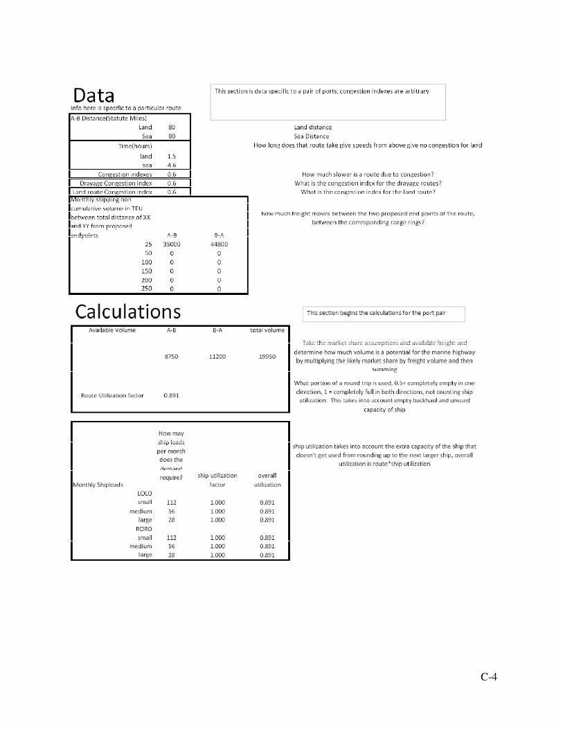
Estimation of the Available Truck Demand

The difficulty with making the model work was getting data for the available demand for freight along a proposed marine highway. For simple routes that are dominated by one parallel highway and short in length, the available demand could be approximated by the eligible traffic count that passes through any point on that parallel highway. Eligible in this context means freight that is not sensitive to the potentially higher latency of a marine highway and traveling along the proposed route. Longer proposed routes present a more difficult problem in gathering demand data because a point based traffic count becomes less accurate of an estimation since it is unknown if the end to end route of the eligible freight at any point pass near both endpoints of the proposed marine highway or if portions of a point based traffic count make intermediate stops that are short of the marine highway endpoints. Put another way, determining the eligible freight on marine highways that bypass major centers of commerce is difficult. The demand is a key element in determining the feasiblity of a short sea shipping route. In this project, demand was estimated by taking the traffic count for trucks along parallel highways and adjusting down that existing flow to reflect freight that would not take the marine highway because of the additional latency. After establishing an estimate for potential demand on the proposed marine highway additional aspects of feasibility were examined such as trip time, fuel consumption and cost.

Although not part of the scope of this project, one might want to consider what distances from a city of interest could be considered for viable freight demand. For example, further research may show that distribution centers that are further than fifty miles from a city of interest should be considered to be not viable. Figures 1-3 below shows the iterations of routes that were selected and the assumed available freight traffic.

10

Figure 1. First Route Option between Richmond, VA and Norfolk, VA

The green circle shows where a traffic sample was taken for the available freight (1,750 trucks per day from Norfolk, VA and 2,240 trucks per day from Richmond, VA).

Figure 2. Second Route Option between Richmond, VA and Norfolk, VA

Alternate route between Richmond, VA and Norfolk, VA where the green circle shows where a traffic sample was taken for the available freight (data did not provide a bi-directional estimate, therefore, it was assumed that there was equal flow-680 trucks per day from Norfolk, VA and 680 trucks per day from Richmond, VA).

11

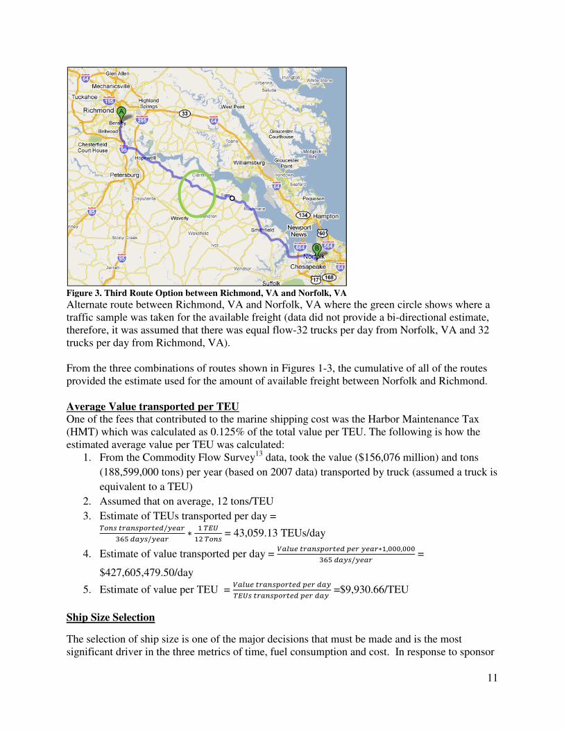
Figure 3. Third Route Option between Richmond, VA and Norfolk, VA

Alternate route between Richmond, VA and Norfolk, VA where the green circle shows where a traffic sample was taken for the available freight (data did not provide a bi-directional estimate, therefore, it was assumed that there was equal flow-32 trucks per day from Norfolk, VA and 32 trucks per day from Richmond, VA). From the three combinations of routes shown in Figures 1-3, the cumulative of all of the routes provided the estimate used for the amount of available freight between Norfolk and Richmond.

Average Value transported per TEU

One of the fees that contributed to the marine shipping cost was the Harbor Maintenance Tax (HMT) which was calculated as 0.125% of the total value per TEU. The following is how the estimated average value per TEU was calculated:

1. From the Commodity Flow Survey13 data, took the value ($156,076 million) and tons

(188,599,000 tons) per year (based on 2007 data) transported by truck (assumed a truck is

equivalent to a TEU)

2. Assumed that on average, 12 tons/TEU

3. Estimate of TEUs transported per day = ���� ���������/ ��

��� �� �/ ��∗

� ���

�� ���� = 43,059.13 TEUs/day

4. Estimate of value transported per day = ���� ��������� � ��∗�,���,���

��� �� �/ �� =

$427,605,479.50/day

5. Estimate of value per TEU = ���� ��������� � ��

���� ��������� � �� =$9,930.66/TEU

Ship Size Selection

The selection of ship size is one of the major decisions that must be made and is the most significant driver in the three metrics of time, fuel consumption and cost. In response to sponsor

12

input, an additional metric of time reliability, derived from the simulation portion of the project, was used as a comparative metric as well. With three objectives at play when selecting ship size a typical method of appropriately making decisions is using Multiple Objective Decision Analysis (MODA).14 For the MODA methodology, a value function for each of the objectives is defined from subject matter experts (SME), weights for each of the objectives are determined and then the weighted value functions are added together and the "best" option can be chosen. The value functions can be as simple as linear functions ranking the worst to the best options as follows:

Where

v(xij) is the value of option j with respect to metric i

xij is the ith metric of option j, and

xi is the vector with the ith metric for all j options.

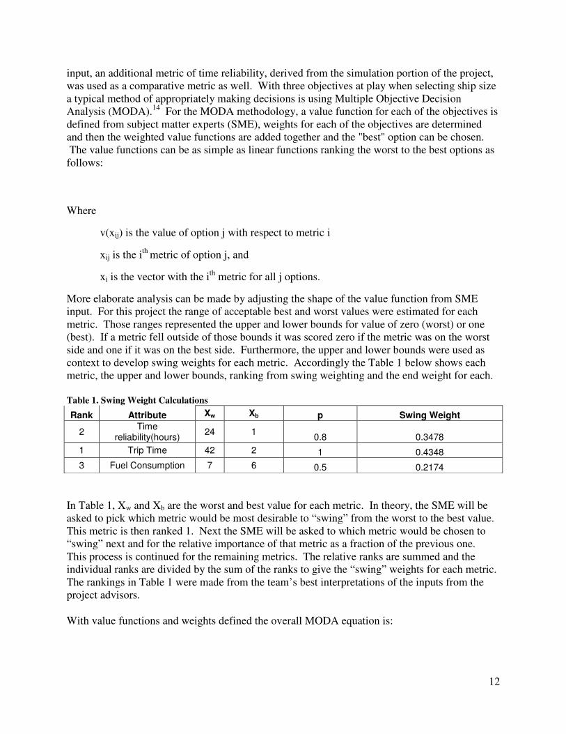
More elaborate analysis can be made by adjusting the shape of the value function from SME input. For this project the range of acceptable best and worst values were estimated for each metric. Those ranges represented the upper and lower bounds for value of zero (worst) or one (best). If a metric fell outside of those bounds it was scored zero if the metric was on the worst side and one if it was on the best side. Furthermore, the upper and lower bounds were used as context to develop swing weights for each metric. Accordingly the Table 1 below shows each metric, the upper and lower bounds, ranking from swing weighting and the end weight for each.

Table 1. Swing Weight Calculations

Rank Attribute Xw Xb p Swing Weight

2 Time

reliability(hours) 24 1

0.8 0.3478

1 Trip Time 42 2 1 0.4348

3 Fuel Consumption 7 6 0.5 0.2174

In Table 1, Xw and Xb are the worst and best value for each metric. In theory, the SME will be asked to pick which metric would be most desirable to “swing” from the worst to the best value. This metric is then ranked 1. Next the SME will be asked to which metric would be chosen to “swing” next and for the relative importance of that metric as a fraction of the previous one. This process is continued for the remaining metrics. The relative ranks are summed and the individual ranks are divided by the sum of the ranks to give the “swing” weights for each metric. The rankings in Table 1 were made from the team’s best interpretations of the inputs from the project advisors.

With value functions and weights defined the overall MODA equation is:

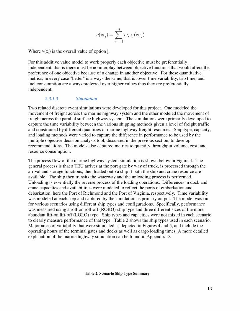
Where v(xj) is the overall value of option j.

For this additive value model to work properly each objective must be preferentially independent, that is there must be no interplay between objective functions that would affect the preference of one objective because of a change in anometrics, in every case "better" is always the same, that is lower time variability, trip time, and fuel consumption are always preferred over higher values thus they are preferentially independent.

2.3.1.3 Simulation

Two related discrete event simulations were developed for this project. One modeled the movement of freight across the marine highway system and the other modeled the movement of freight across the parallel surface highway system. Thecapture the time variability between the various shipping methods given a level of freight traffic and constrained by different quantities of marine highway freight resources. Ship type, capacity, and loading methods were varied to capture the difference in performance to be used by the multiple objective decision analysis tool, discussed in the previous section, to develop recommendations. The models also captured metrics to quantify throughput volume, cost, and resource consumption.

The process flow of the marine highway system simulation is shown below in Figure 4. The general process is that a TEU arrives at the port gate by way of truck, is processed through the arrival and storage functions, then loaded onto a ship if both the shavailable. The ship then transits the waterway and the unloading process is performed. Unloading is essentially the reverse process of the loading operations. Differences in dock and crane capacities and availabilities were moddebarkation, here the Port of Richmond and the Port of Virginia, respectively. Time variability was modeled at each step and captured by the simulation as primary output. The model was run for various scenarios using different ship types and configurations. Specifically, performance was measured using a roll-on rollabundant lift-on lift-off (LOLO) type. Ship types and capacities were not mixed in eacto clearly measure performance of that type. Table 2 shows the ship types used in each scenario. Major areas of variability that were simulated as depicted in Figures 4 and 5, and include the operating hours of the terminal gates and docks as wexplanation of the marine highway simulation can be found in Appendix D.

Table

lue of option j.

For this additive value model to work properly each objective must be preferentially independent, that is there must be no interplay between objective functions that would affect the preference of one objective because of a change in another objective. For these quantitative metrics, in every case "better" is always the same, that is lower time variability, trip time, and fuel consumption are always preferred over higher values thus they are preferentially

Simulation

Two related discrete event simulations were developed for this project. One modeled the movement of freight across the marine highway system and the other modeled the movement of freight across the parallel surface highway system. The simulations were primarily developed to capture the time variability between the various shipping methods given a level of freight traffic and constrained by different quantities of marine highway freight resources. Ship type, capacity,

ds were varied to capture the difference in performance to be used by the multiple objective decision analysis tool, discussed in the previous section, to develop recommendations. The models also captured metrics to quantify throughput volume, cost, and

The process flow of the marine highway system simulation is shown below in Figure 4. The general process is that a TEU arrives at the port gate by way of truck, is processed through the arrival and storage functions, then loaded onto a ship if both the ship and crane resource are available. The ship then transits the waterway and the unloading process is performed. Unloading is essentially the reverse process of the loading operations. Differences in dock and crane capacities and availabilities were modeled to reflect the ports of embarkation and debarkation, here the Port of Richmond and the Port of Virginia, respectively. Time variability was modeled at each step and captured by the simulation as primary output. The model was run

s using different ship types and configurations. Specifically, performance on roll-off (RORO)-ship type and three different sizes of the more

off (LOLO) type. Ship types and capacities were not mixed in eacto clearly measure performance of that type. Table 2 shows the ship types used in each scenario. Major areas of variability that were simulated as depicted in Figures 4 and 5, and include the operating hours of the terminal gates and docks as well as cargo loading times. A more detailed explanation of the marine highway simulation can be found in Appendix D.

Table 2. Scenario Ship Type Summary

13

For this additive value model to work properly each objective must be preferentially independent, that is there must be no interplay between objective functions that would affect the

For these quantitative metrics, in every case "better" is always the same, that is lower time variability, trip time, and fuel consumption are always preferred over higher values thus they are preferentially

Two related discrete event simulations were developed for this project. One modeled the movement of freight across the marine highway system and the other modeled the movement of

simulations were primarily developed to capture the time variability between the various shipping methods given a level of freight traffic and constrained by different quantities of marine highway freight resources. Ship type, capacity,

ds were varied to capture the difference in performance to be used by the multiple objective decision analysis tool, discussed in the previous section, to develop recommendations. The models also captured metrics to quantify throughput volume, cost, and

The process flow of the marine highway system simulation is shown below in Figure 4. The general process is that a TEU arrives at the port gate by way of truck, is processed through the

ip and crane resource are available. The ship then transits the waterway and the unloading process is performed. Unloading is essentially the reverse process of the loading operations. Differences in dock and

eled to reflect the ports of embarkation and debarkation, here the Port of Richmond and the Port of Virginia, respectively. Time variability was modeled at each step and captured by the simulation as primary output. The model was run

s using different ship types and configurations. Specifically, performance ship type and three different sizes of the more

off (LOLO) type. Ship types and capacities were not mixed in each scenario to clearly measure performance of that type. Table 2 shows the ship types used in each scenario. Major areas of variability that were simulated as depicted in Figures 4 and 5, and include the

A more detailed

14

Scenario Ship Type TEU Capacity

1 RORO 100

2 RORO 200

3 LOLO 100

4 LOLO 200

Figure 4. Marine Highway Simulation Flow Diagram

The surface transportation simulation flow is depicted in Figure 5. The truck-borne TEU starts as if it just left the gate of a marine terminal. It then travels surface routes to the gate of its destination marine terminal. These start and end points are essentially the same as for the marine highway to allow for comparison. Route segment length, traffic volume, and accident statistics were incorporated into the routes to propagate and capture delays. Roadway statistics were taken from 2008 data published by the US Department of Transportation. In the case of transport from

TEU arrives at port gate

Ship arrives at port

Ship departs

TEU loaded on ship

Ship transits water route

TEU moved to storage

TEU trucked to warehouse

Ship released

TEU unloaded to

trucks

Ship arrives at port

15

the Port of Richmond to the Port of Virginia, there are several equivalent routes for a truck-borne TEU to travel. The route used in any given simulation run is chosen by the user. This simulation captured the time variability of the end-to-end transportation process as well as statistics for fuel and road maintenance costs associated with the freight traffic.

Figure 5. Surface Highway Simulation Flow Diagram

2.3.1.4 Analysis

Early on in the project one goal was to reduce congestion on the highways by redirecting freight to short sea shipping. A survey of the existing body of work revealed that a best case scenario was to move 500 trucks off the highway system per day. Knowing that the capacity of 2 lanes of highway is roughly 700 trucks per hour it was evident that removing 500 trucks per day from a highway would not yield significant congestion reduction benefits. If marine highways were to become viable then other motivations needed to be promoted in addition to congestion reduction. There was a challenge when deciding on how best to analyze and show the results. Additionally, although this project focused on a small scale route, the methodology was developed to be fleixble enough for eventual scaling, therefore, the analysis needed to be equivalently flexible in nature to support the eventual scalability. The scalability of the simulation is fairly straight forward but, for reasons already mentioned, scalability of method used to determine the available demand is more difficult (reference to “Follow-on Work” section).

TEU generated at

starting warehouse

Transit surface route

Determine route

TEU arrives at destination warehouse

16

17

3 Results

Simulation results and decision analysis tool results are both presented here to give insight to the feasibility of a marine highway that would parallel I-64 between Richmond and Norfolk.

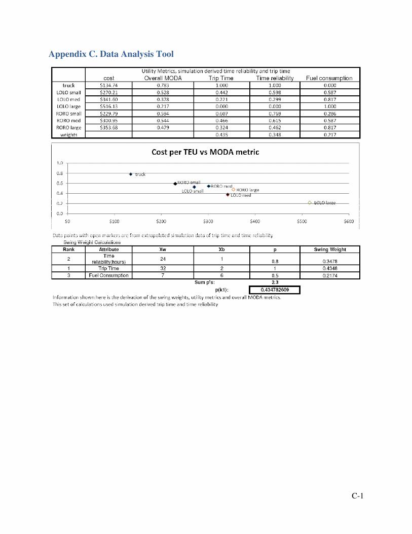
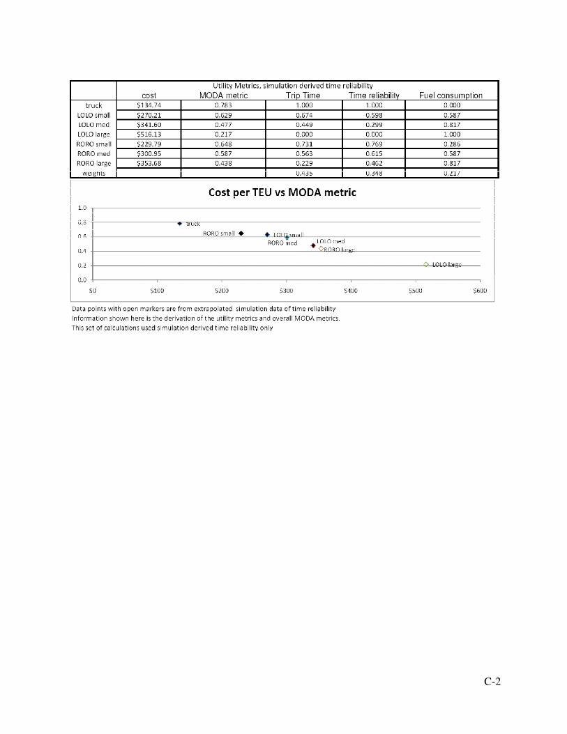
3.1 Decision Analysis Tool Deliverables and Results

With estimates of the time reliability from the simulation an overall MODA metric was developed. As detailed in the simulation section above, 4 options were simulated: small and medium, LOLO and RORO ships. Small is a capacity of 100 TEU’s and Medium is a capacity of 400 TEU’s. These results were interpolated to approximate metrics for a large capacity ship in both LOLO and RORO configuration. Those data points are detailed with an open diamond where as the data points based on simulation data are filled in black triangles.

Figure 6. Cost per TEU versus MODA Metric

MODA Metrics for 6 options, James River, 80 mile Marine Highway. note: Data points with open markers were from extrapolated simulation data of trip time and time reliability.

Table 3. Raw Metrics Used to Derive MODA Metrics

Trip time and time reliability were derived from simulations while fuel consumption was calculated.

LOLO small

LOLO med LOLO large

RORO small

RORO med

RORO large

truck

0.0

0.2

0.4

0.6

0.8

1.0

$0 $50 $100 $150 $200 $250 $300 $350 $400 $450

Util

ity

Cost per TEU vs MODA metric w/ gate hrs and 1 crane

18

Plainly from the Figure 6 and Table 3, the best option is to truck freight rather than try to utilize a marine highway for this short, 80 mile, route. Simply put the greater efficiency of moving freight on a ship is not taken advantage of for long enough to overcome the fixed costs associated with moving the cargo through the port. Additionally, gate hours, the time when the ports operate, are a major driver for trip time, 24 hour operations would allow much greater throughput and shorter trip times. Figure 7 provides a notional example of realxing the constraints by assuming 24 hours gate operations and the addition of an extra crane. For this case the time reliability is taken from the previous 80 mile simulation and the other metrics of trip time and fuel consumption are derived from deterministic calculations.

Figure 7. Cost per TEU versus MODA Metric (24 hour gate operations and 2 cranes)

MODA metrics for 7 options with relaxed constraints, calculated trip time, cost and fuel consumption. Time reliability is taken from James River simulation. note: Data points with open markers are from extrapolated simulation data of time reliability.

Table 4. Raw Metrics Used to Derive MODA Metrics (24 hour gate operations and 2 cranes)

Raw metrics used to derive MODA metrics for relaxed terminal operations. Time reliability was derived from the simulation while fuel consumption and trip time were calculated. Note: due to

Utility Metrics, simulation derived time reliability and trip time

Cost Utility Trip Time Time reliability Fuel consumption

Truck $65 0.865 0.988 0.983 0.430

LOLO small $252 0.551 0.190 0.807 0.617

LOLO med $264 0.220 0.000 0.152 0.706

LOLO large $389 0.169 0.000 0.000 0.777

RORO small $176 0.588 0.344 0.828 0.501

RORO med $223 0.209 0.000 0.172 0.617

RORO large $416 0.154 0.000 0.000 0.706

weights 0.348 0.435 0.217

LOLO small

LOLO medLOLO large

RORO small

RORO medRORO large

Truck

0.0

0.2

0.4

0.6

0.8

1.0

$0 $50 $100 $150 $200 $250 $300 $350 $400 $450

Util

ity

Cost per TEU vs MODA metric w/ no gate hrs and 2 crane

19

limitations of the decision analysis tool no gate hours were accounted for thus the trip times reflect 24 hour operations and are optimistically short.

From Figure 7 and Table 4, a Marine Highway with relaxed constrains, shows good promise of competing in cost terms with standard trucking (Figure 6 and Table 3) from the perspective of the MODA metrics chosen in this analysis although trip time was still significantly larger than an all truck route. The column highlighted in yellow shows the percentage utility improvement due to the relaxed terminal operations. Although the truck is still the most promising as far as utility, the marine options increase significantly in utility. However, the cost competiveness is still not comparable to the trucks.

3.2 Simulation Deliverables and Results

Several simulations of the road and marine networks were completed for the analysis. After compiling the results, the marine highway did not perform as well as the surface route in either time reliability or cost, which may be expected on such a short sea route. However, this doesn’t mean that the marine highway is not viable. As mentioned in the preceding section, the marine highway may become more economical over longer routes, where the surface route begins to encounter more significant and more unpredictable delay times, and the stability of the marine route can be realized. That said, in the case of I-64, while the marine highway did not perform as well as the surface routes, consider that some of the ship types possessed time reliability within 2-4 hours. Though not as good as the surface route, this is still a rather small window, perhaps small enough to make a decision maker indifferent about the range of variation. More research would need to be conducted with shippers and DOT decision makers to determine exactly what the preferences are for the range of variation on these attributes.

Another observation resulting from our simulations is that the limited operating hours of the terminal make it somewhat less flexible than the surface route. Consider that a container arriving in Port of Virginia late in the afternoon may be offloaded, but not able to be picked up by a truck to depart the terminal until the following day. Containers travelling by surface route did not encounter such delays. In real life, some of this effect is mitigated by the fact that shippers maintain private storage facilities within the terminal to provide them more flexibility. However, this level of detail was not in the scope of our project.

Finally, the simulations can provide the building blocks for comparisons between any two ports. Demand data for containers will need to be researched to include in the models, but the basic

Utility Metrics, simulation derived time reliability and trip time

Cost Utility % Improvement Trip Time Time reliability Fuel consumption

Truck $65 0.865 0% 0.988 0.983 0.430

LOLO small $252 0.716 30% 0.467 0.966 0.617

LOLO med $264 0.631 187% 0.225 0.917 0.706

LOLO large $389 0.547 224% 0.000 0.869 0.777

RORO small $176 0.685 16% 0.459 0.959 0.501

RORO med $223 0.631 202% 0.248 0.945 0.617

RORO large $416 0.571 272% 0.037 0.931 0.706

weights 0.348 0.435 0.217

20

elements of a terminal operation or surface route are present such that resource capacities, process times and delays can be scaled to suit any port. Of course with more time and resources, more detail can be added to the simulations to provide a more rigorous answer. But as an initial test of viability, we are confident that our simulation serves its purpose.

21

22

4 Discussion

Short sea shipping has various obstacles to overcome in order to become viable. First is the Jones Act, also known as the Merchant Marine Act of 192015, which requires ships that engage in intra US commerce to be US built and crewed by predominantly US personnel. The purpose of the act is to keep the US shipbuilding industry alive but as other countries have developed industrial capacity the US industry has fallen behind in cost, quality and volume. Short sea shipping could revitalize the US shipbuilding but the shipbuilding industry will need to build ships that are of the same quality, efficiency and cost as are available on the international market in order to make marine highway viable.

Calculations from the decision analysis tool have revealed that routes need to be longer than the James River route that has been analyzed in depth. Longer routes take advantage of the higher efficiency of a ship versus truck efficiency, that efficiency gain is necessary to overcome the costs and time delays associated with the transshipment of freight. Additionally the simulation comparison between truck and ship shows that for short routes the highway offers more consistent trip times. Longer routes may show variability that is comparatively less than the ship alternative. For the purposes of this project, per advisor direction, the team decided to operate under the assumption that trip time is not as significant of a driver for freight shipping but validation needs to be done to determine market sensitivity to longer shipping times as well.

Additional obstacles to short sea shipping are the gate hours present at ports. Freight shipping is generally a 24 hour operation and for short sea shipping to compete with standard trucking and railway shipping then ports will need to adopt extended hours. The gate hours also concentrate freight operations around the port during what are also peak congestion hours which is counter to some of the goals of short sea shipping. The simulation in this project took into account gate hours and subsequently the trip time and time reliability were adversely affected.

23

24

5 Conclusions

5.1 Observations It is possible that short sea shipping is not viable on its own fiscal merits but it still offers public benefits. Therefore, incentives and policy reform may be warranted to make the marine highway more attractive. For example, subsidies may be necessary to revitalize the shipbuilding industry so that US shipyards can build ships that are competitive on a global scale. The justification for these subsidies can be derived from the highway maintenance cost avoidance associated with decreasing truck travel on the highway system. Additionally, the harbor maintenance tax (HMT) applied to the value of all cargo that transits each port may be cost inhibitive for a shipper or manufacturer to consider short sea shipping. However, offering incentives such as HMT fee discounts or waiving or creating tolls or fees for trucks that travel during peak traffic times could assist in a shift in modes. Some examples of policy reform could include mandating that a specific percentage of freight (based on annual volume, frequency of trips, etc) is required to travel via a more fuel efficient or “green” way. Additionally if congestion reduction is a goal of short sea shipping, the gate hours at ports need to be adjusted to allow for 24 hr operations such that freight can be transferred to a marine highway outside of peak congestion hours.

Longer routes may provide more promising results for the marine highway, some rough estimates from this study show approximately between 400 and 600 miles might be around the break-even point.

Congestion reduction is most likely not significant based on this project, however, congestion avoidance would be a significant motivation for shippers.

The following is a summary of the overall recommendations to promote the transfer of freight from surface to marine highways:

• Increase utility – Move to 24-hour operations – Increase terminal throughput

• Increase cost competitiveness – Provide tax incentives or subsidies for use of marine highway – Re-evaluate harbor maintenance tax

• Policy reforms – Mandate certain % of freight use “greener” modes of transport

5.2 Follow on work As mentioned earlier, one of the primary issues was the data available for county to county traffic and freight demand. This data is essential for the initial viability “litmus test.” For example, the Commonwealth of Virginia DOT publishes a document (“Average Daily Traffic Volumes with Vehicle Classification Data on Interstate, Arterial, and Primary Routes”) which provide highly detailed traffic data broken out by vehicle type, weekday versus overall average, and in some cases, bi-directional flow. However, there is a lack of direct data that measures traffic flow by type that goes between counties or cities of interest. Alternatively, the US Census Bureau provides extensive commodity flow data based on surveys which can be viewed by mode

25

of transportation, commodity, and regional area. However, this data appears to provide point to point traffic information assuming that the freight originated from city A and flows to city B. Data that is missing is the freight that did not originate from city A, but may be passing within some distance from A to end or travel through city B. Therefore, the first recommendation for follow on work would be to compile a wider range of data sources (e.g., for multiple states) and then build the data architecture for the county to county traffic/freight data.

An additional method of testing viability is through sensitivity analysis. Through the use of sensitivity analysis, it is feasible that there would be a threshold for which marine highway would prove to be the most efficient (time, throughput, fuel, cost, etc) if a specific distance or ship capacity is reached.

Another possible avenue to explore would be to modify the model by developing a graphic user interface (GUI) or utilizing Visual Basic Application (VBA) code to provide input screens for the user to provide options prior to running the simulation. For example, tables could be created to document ship types which could include specifications like:

• Dimensions

• Container capacity (e.g., TEUs via LoLos or RoRos)

• Fuel consumption

• Speed

Similarly, a table for port specifications could be created to include:

• Number and type of cranes

• Crane capacity (load/unload capability)

• Crane reach

• Terminal dimensions (number of berths, main channel leading into terminal, number of piers)

• Types of cargo

• Storage capacity

• Costs (loading/unloading, storage, etc)

Finally, developing an estimate for the “savings” in congestion was too complex for the scope of this project, therefore, the congestion and road maintenance aspects should be explored more in depth for more detailed incorporation. As shown earlier, one of the outputs of the model is the TEU throughput which provided an estimate of the number that could be removed from highways. The complexity increases when attempting to measure the impact on a commuter’s congestion time due to the fact that TEUs being transferred to the marine highway will result in more traffic of other types to replace it. More in depth research should be explored on the vast traffic related data (e.g., volume, density, average time between points or mile markers) to include accident rates, hazardous material safety issues, and more detail on the relationship between road maintenance and freight traffic versus other traffic. The following is a summary of the recommended future work to continue efforts to transfer of freight from surface to marine highways:

26

• Simulation • Model multiple terminals • Expand the list of routes (marine and highway)

• Decision Analysis Tool • Consider other attributes for MODA • Research congestion metrics

• Architecture • Data feeds • Graphical User Interface

A-1

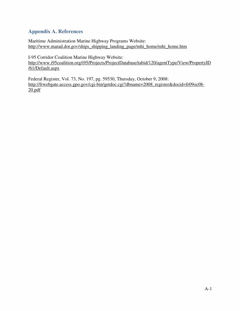
Appendix A. References

Maritime Administration Marine Highway Programs Website: http://www.marad.dot.gov/ships_shipping_landing_page/mhi_home/mhi_home.htm I-95 Corridor Coalition Marine Highway Website: http://www.i95coalition.org/i95/Projects/ProjectDatabase/tabid/120/agentType/View/PropertyID/61/Default.aspx Federal Register, Vol. 73, No. 197, pg. 59530, Thursday, October 9, 2008: http://frwebgate.access.gpo.gov/cgi-bin/getdoc.cgi?dbname=2008_register&docid=fr09oc08-20.pdf

B-1

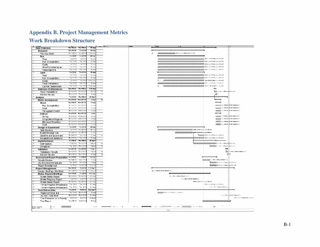
Appendix B. Project Management Metrics

Work Breakdown Structure

B-2

Earned Value management

$0.00

$5,000.00

$10,000.00

$15,000.00

$20,000.00

$25,000.00

$30,000.00

$35,000.00

BCWS

ACWP

BCWP

C-1

Appendix C. Data Analysis Tool

C-2

C-3

C-4

C-5

C-6

C-7

C-7

D-1

Appendix D. Simulation

Surface Transportation Simulation

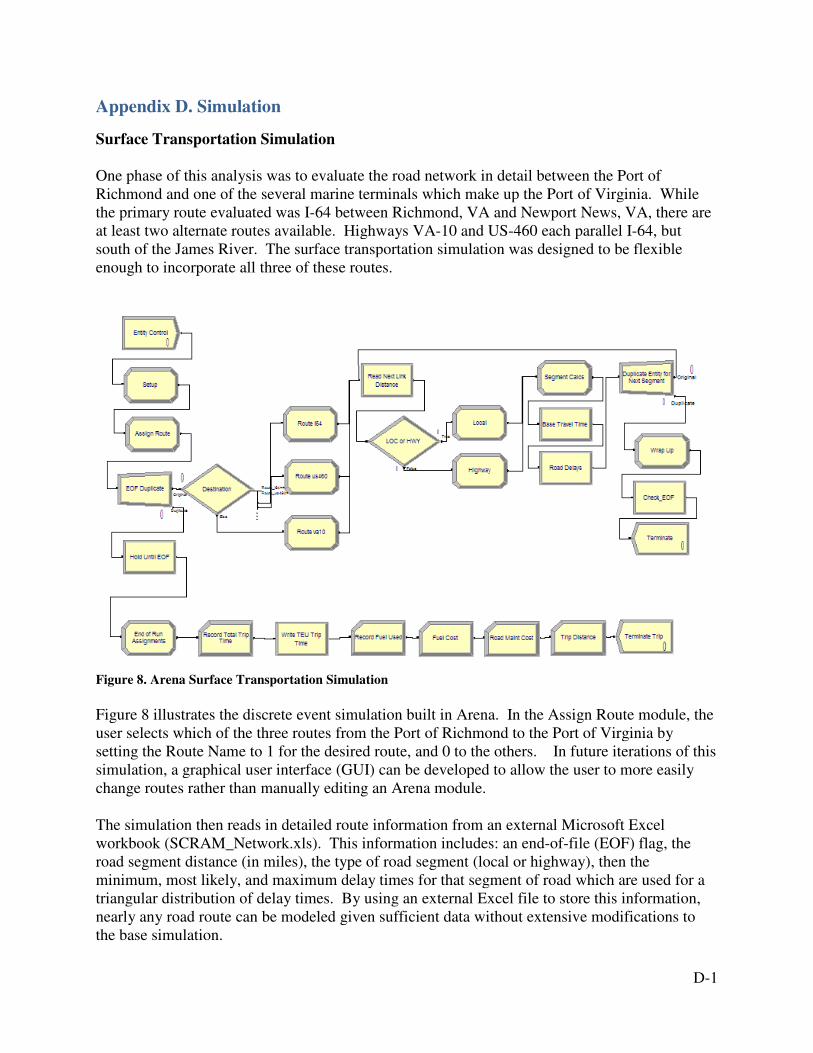
One phase of this analysis was to evaluate the road network in detail between the Port of Richmond and one of the several marine terminals which make up the Port of Virginia. While the primary route evaluated was I-64 between Richmond, VA and Newport News, VA, there are at least two alternate routes available. Highways VA-10 and US-460 each parallel I-64, but south of the James River. The surface transportation simulation was designed to be flexible enough to incorporate all three of these routes.

Figure 8. Arena Surface Transportation Simulation

Figure 8 illustrates the discrete event simulation built in Arena. In the Assign Route module, the user selects which of the three routes from the Port of Richmond to the Port of Virginia by setting the Route Name to 1 for the desired route, and 0 to the others. In future iterations of this simulation, a graphical user interface (GUI) can be developed to allow the user to more easily change routes rather than manually editing an Arena module.

The simulation then reads in detailed route information from an external Microsoft Excel workbook (SCRAM_Network.xls). This information includes: an end-of-file (EOF) flag, the road segment distance (in miles), the type of road segment (local or highway), then the minimum, most likely, and maximum delay times for that segment of road which are used for a triangular distribution of delay times. By using an external Excel file to store this information, nearly any road route can be modeled given sufficient data without extensive modifications to the base simulation.

D-2

Once the end-of-file is reached, the final values of key variables (total trip time, distance traveled, fuel used, total fuel cost, and road maintenance costs) are recorded and the total trip time is written to a second external Excel file (SCRAM_Output.xls). In this file, the minimum, maximum, mean, and standard deviation are calculated. The other key variables are held in the Arena .out output file.

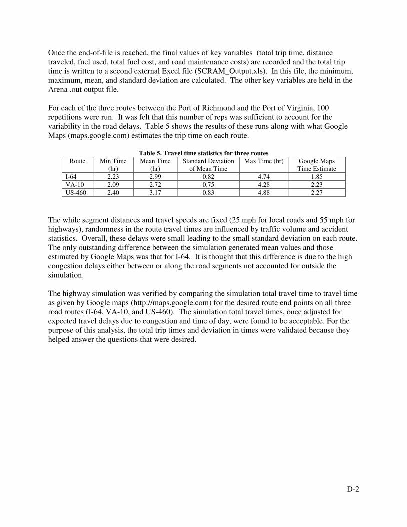
For each of the three routes between the Port of Richmond and the Port of Virginia, 100 repetitions were run. It was felt that this number of reps was sufficient to account for the variability in the road delays. Table 5 shows the results of these runs along with what Google Maps (maps.google.com) estimates the trip time on each route.

Table 5. Travel time statistics for three routes

Route Min Time (hr)

Mean Time (hr)

Standard Deviation of Mean Time

Max Time (hr) Google Maps Time Estimate

I-64 2.23 2.99 0.82 4.74 1.85

VA-10 2.09 2.72 0.75 4.28 2.23

US-460 2.40 3.17 0.83 4.88 2.27

The while segment distances and travel speeds are fixed (25 mph for local roads and 55 mph for highways), randomness in the route travel times are influenced by traffic volume and accident statistics. Overall, these delays were small leading to the small standard deviation on each route. The only outstanding difference between the simulation generated mean values and those estimated by Google Maps was that for I-64. It is thought that this difference is due to the high congestion delays either between or along the road segments not accounted for outside the simulation.

The highway simulation was verified by comparing the simulation total travel time to travel time as given by Google maps (http://maps.google.com) for the desired route end points on all three road routes (I-64, VA-10, and US-460). The simulation total travel times, once adjusted for expected travel delays due to congestion and time of day, were found to be acceptable. For the purpose of this analysis, the total trip times and deviation in times were validated because they helped answer the questions that were desired.

D-2

D-3

Port Simulations

Figure 9. Arena Port of Richmond Simulation

Figure 9 shows the portion of the simulation that represents operations at the Port of Richmond terminal. In the segment labeled “Container Arrival to Port of Richmond,” trucks carrying containers arrive at the gate. The truck arrival gate at Port of Richmond is open only between the hours of 0800 and 1700, and closed for one hour during lunch. Therefore, trucks arriving outside of these times will need to wait for the gate to open. Once through the gate, the truck will deliver its container to the storage facility, and then depart the terminal. There is a nominal time associated with the process of getting through the gate for credential validation and delivery to the storage yard, between 12-15 minutes on average. Next, in the segment labeled “Port of Richmond Terminal Operations,” ships arrive to the port each morning to pick-up TEUs according to their capacity. This operation is independent of the container arrival process, therefore, it is possible that a ship may depart the port carrying less than its full capacity. If the ship type is a LoLo, then a crane will be required for the onload operations. With the current limitations on gate and dock operating hours, it was deemed impractical to exsect more than ship to be able to onload its cargo per day. Therefore, while appropriately incorporated into the model, the crane resource was never unavailable to an arriving ship. This feature may be useful in modeling busier ports where multiple ships can be loaded each day. The RoRo does not require a crane and can begin its onload operations upon arriving dockside. Depending on the ship type and its capacity, each ship will load the smaller of the number of containers present in the storage yard and its full capacity, at the appropriate loading rate. After onload operations, the ship releases the dock and crane resources, and makes way for the Port of

Docking Time

Undocking TimeLabor TimeRecord PoR Crane

Depart PoRRelease P oR Dock

Create Arriving LoLo

PoRStart Crane Labor at

LoLo Arrival at PoR

Port of Richmond Terminal Operations

Container Arrival to Port of Richmond

Pierside Richmond

S tation PoRS hip Loading

PoR Trucks PoR Assignments PoR Gate

StoragePort of Richmond

PoR LotAdd Container to

Container LotS eize PoR

Container LotRelease PoR

RegulatorSeize P oR Flow LoLo

3Release Regulator

CraneRelease PoR

Seize Crane P oR

Seize PoR Dock

Ops TimeRecord PoR Ship

CapacityAssign Ship

Unloaded at PoRContainers

on ShipsCount Containers

TimeRecord Truck Ops

Dispose Truck

0

0

0

0

0

0

D-4

Virginia via the James River. The marine route was modeled with little variability to account for possible heavy traffic near the ports and weather.

Figure 10. Arena Port of Virginia Simulation

Figure 10 is the simulation for the “Port of Virginia Terminal Operations.” The logic is similar to Port of Richmond (Figure 9). Since operations at Port of Richmond are on a much smaller scale than Port of Virginia, the available resources at Port of Virginia could easily handle the inbound shipments. However, like Port of Richmond, the primary constraints were the operating hours of the departure gate and docks.

Much like Port of Richmond, docks and cranes were utilized as appropriate to offload the containers into the storage yard, after which the ship was disposed. Finally, trucks arriving regularly to the gate retrieve a container before departing the terminal.

Primary output metrics collected from this simulation were total container time in transit, standard deviation of this time, as well as resource utilization time for cranes and docks to which costs can be applied for a total cost comparison.

Dock ing PoV

PoVUndock ing Time

Labor TimeRecord PoV Crane

Dispose Ship EntityRelease PoV Dock

PoVStart Crane Labor at

LoLo Arrival at PoV

Port of Virginia Terminal Operations

Piers ide PoV

Station PoV

Ship Loading

StoragePort of Vi rginia

Regulator

Seize PoVFlow LoLo PoV

5

Release RegulatorCrane

Releas e PoV

Seize Crane PoV

Port of Vi rginia Seize PoV Dock

Loading OpsRecord PoV Truck

Record StDev

Container Departure from Port of Virginia

Truck Arrives PoVAssignmentsPoV Truck

Truck Departs PoV

PoV Gate

from PoV LotRemove Container

Container LotSeize PoV

Container LotRelease PoV

Leaving PoVCount Containers

Travel TimeRecord Container

PoV Load to Truck

Ops TimeRecord PoV Ship

TimeTotal Container

TruckHold for Trigger

ReleaseTrigger Truck

Chec k Gate QueueTr ue

False

Check Storage LevelTr ue

False

ContainersRecord Outbound

0

0

0

0

0

0

0

0

0

D-5

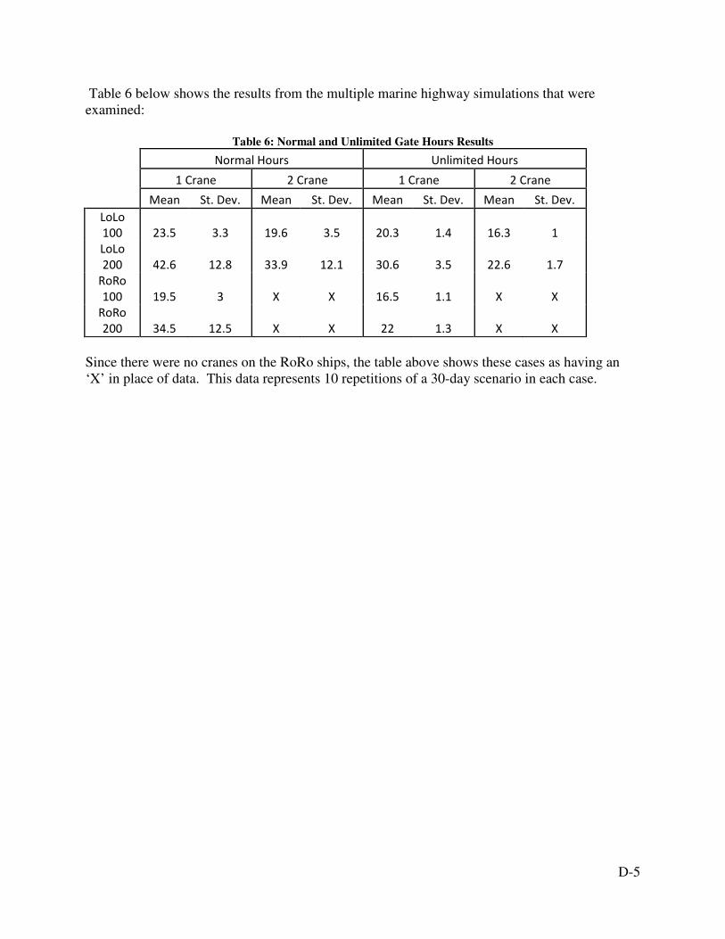
Table 6 below shows the results from the multiple marine highway simulations that were examined:

Table 6: Normal and Unlimited Gate Hours Results

Normal Hours Unlimited Hours

1 Crane 2 Crane 1 Crane 2 Crane

Mean St. Dev. Mean St. Dev. Mean St. Dev. Mean St. Dev.

LoLo

100 23.5 3.3 19.6 3.5 20.3 1.4 16.3 1 LoLo

200 42.6 12.8 33.9 12.1 30.6 3.5 22.6 1.7 RoRo

100 19.5 3 X X 16.5 1.1 X X RoRo

200 34.5 12.5 X X 22 1.3 X X

Since there were no cranes on the RoRo ships, the table above shows these cases as having an ‘X’ in place of data. This data represents 10 repetitions of a 30-day scenario in each case.

End Notes

1 http://isddc.dot.gov/OLPFiles/OST/012988.pdf 2 http://www.marad.dot.gov/ships_shipping_landing_page/mhi_home/mhi_home.htm 3 http://www.fhwa.dot.gov/policy/otps/freight.pdf 4 http://www.marad.dot.gov/ships_shipping_landing_page/mhi_home/mhi_home.htm 5 http://www.marad.dot.gov/ships_shipping_landing_page/mhi_home/mhi_home.htm 6 Mr. Alexander Landsburg, Senior Member Advisory Staff, CSC Advanced Marine Center 7 February 2, 2010 Email from Dr. Chun-Hung Chen 8 Author Unknown, (15 October 2009) Induced demand, From Wikipedia, the free encyclopedia, Retrieved from: http://en.wikipedia.org/wiki/Induced_demand. 9 Joseph Darcy, Short Sea Shipping: Barriers, Incentives and Feasibility of Truck Ferry, 2009, page 77 10 Global Insight, Four Corridors Case Study of Short-Sea Shipping Services, (submitted to US Department of Transportation, Office of the Secretary/Maritime Administration), August 2006, page 33 11 National Cooperative Highway Research Program, Multimodal corridor and capacity analysis manual Issue 399, (Transportation Research Board, 1998) page 83 12 US Maritime Administration, Americas ports and Intermodal transportion system, January 2009, Page 33 13 www.bts.gov/publications/commodity_flow_survey/ 14 Andrew G. Loerch, Larry B Rainey, Methods for Conducting Military Operational Analysis, (Military Operations Research Society, 2007), 628-629. 15 Author Unknown, (2 May 2010) Merchant Marine Act of 1920, From Wikipedia, the free encyclopedia, Retrieved from: http://en.wikipedia.org/wiki/Induced_demand.