THE IMPACT OF MONETARY POLICY ON INCOME AND WEALTH

163The Distributional Impact of Monetary Policy in SEACEN Member Economies

CHAPTER 7

THE IMPACT OF MONETARY POLICY ON INCOME AND WEALTH DISTRIBUTION:

A CASE OF THAILANDBy

Passakorn Tapasanan and Piraya Ronaparp1

1. Introduction

Not long after experiencing the financial crisis, Thailand adopted a flexible inflation targeting regime from May 2000, a change from the long implemented exchange rate targeting framework, which followed a brief period of monetary targeting regime2. Since then, Thailand has been able to achieve price stability, where core inflation moves favorably within the target range3 most of the time (Chart 1). Of late, however, when Thailand changed the target of core inflation to headline inflation, it has fallen uncomfortably short of the lower bound of the target range. Despite this shortfall, Thailand has still been able to maintain price stability along with its coherent objectives of supportive economic growth and a sound financial system.

Chart 1 Inflation and Inflation Target Range

1. The Bank of Thailand, Email: [email protected] or [email protected]. All views expressed are solely those of authors and cannot be taken to represent those of the Bank of Thailand or the SEACEN Centre.

2. Bank of Thailand was founded in 1942. It first adopted the pegged exchange rate regime (Second World War - June 1997), and briefly adopted the monetary targeting regime (July 1997 - May 2000) after floating the exchange rate. https://www.bot.or.th/English/MonetaryPolicy/MonetPolicyKnowledge/Pages/Framework.aspx

3. Since the adoption of flexible inflation targeting regimes, Thailand has had multiple target ranges throughout its history. Core inflation target at 0-3.5% (May 2000 – Dec 2008), Core inflation target at 0.5-3.0% (2009 - 2014), and Headline inflation target at 2.5% with a tolerance band of 1.5% (2015 to present). https://www.bot.or.th/English/MonetaryPolicy/MonetPolicyKnowledge/Pages/Target.aspx

%

mailto:[email protected]

mailto:[email protected]

https://www.bot.or.th/English/MonetaryPolicy/MonetPolicyKnowledge/Pages/Framework.aspx

https://www.bot.or.th/English/MonetaryPolicy/MonetPolicyKnowledge/Pages/Framework.aspx

https://www.bot.or.th/English/MonetaryPolicy/MonetPolicyKnowledge/Pages/Target.aspx

https://www.bot.or.th/English/MonetaryPolicy/MonetPolicyKnowledge/Pages/Target.aspx

The Distributional Impact of Monetary Policy in SEACEN Member Economies164 The Distributional Impact of Monetary Policy in SEACEN Member Economies The SEACEN CentreThe Impact of Monetary Policy on Income and Wealth Distribution:

A Case of Thailand

From a macro perspective, effective conduct of monetary policy in Thailand, through price stability and economic growth, is widely acknowledged. Yet few evidences point to its effectiveness from a micro perspective, particularly on household income and wealth. There is still a need for researchers to investigate this area. However, an in-depth exploration at the individual household level, rich micro-data source is required. Since 2007, Thailand has been conducting revised household surveys4, which comprise detailed household level data, including a variety of perspectives on income source and wealth.

To fully exploit available household level micro-data, our analysis follows the framework used in certain researches, but adapts the approaches to make it appropriate for the context of Thailand. The analysis begins with finding the relationship and the impact of monetary policy, particularly the policy rate, on aggregate economic variables; namely GDP, CPI, house price, stock price, yield, and effective rates. Once known, the impact will then be distributed into the household surveys, mainly classified into three different channels. The first channel considers the earnings composition of household from wage and business profits. The second channel is the saving remuneration channel, focusing on net financial position of households, both net savers and borrowers. The third channel is the asset price channel, through capital gains that each household earns from financial assets. After the impact on all available households is distributed, it is compiled into quintiles. This would distinguish the difference across groups, and allows us to determine which channel is the most effective.

From a macro perspective, the results obtained from our SVAR model are

consistent with conventional macroeconomic theories which state that expansionary monetary policy produces a positive impact on output and prices, whilst negatively affects bond yields and effective rates. In terms of the distributional impact of monetary policy, it is found that wealthy households are more sensitive to monetary policy shocks through asset price and earnings composition channel, based on the assumption that the SVAR model yields symmetric results for contractionary and expansionary monetary policy. This supports the notion that the implementation of expansionary monetary policy may increase income and wealth inequality. Our study also makes a remark about aged citizens who are likely to lose from a lowering of the policy rate as net savers, unlike others who receive benefits as net borrowers.

The remainder of the paper is organized as follows. Section 2 provides the literature review regarding the distributional impact of monetary policy on income and wealth in other countries, along with research on the impact of monetary policy on the Thai economy. Section 3 describes the framework, data, and approaches taken to study the distributional impact of monetary policy in Thailand. Section 4 shows the results of the impact of monetary policy on the aggregate economy using SVAR analysis. Section 5 shows results of the study through the lens of income, wealth and age distribution. Section 6 provides further discussions on consumption, housing, and household debt to provide a better understanding of the behavior of Thai households. Finally, Section 7 concludes.

4. “Household Socio-Economic Survey”. http://www.nso.go.th/sites/2014en/Pages/survey/Social/Household/The-2017-Household-Socio-Economic-Survey.aspx

http://www.nso.go.th/sites/2014en/Pages/survey/Social/Household/The-2017-Household-Socio-Economic-Survey.aspx

http://www.nso.go.th/sites/2014en/Pages/survey/Social/Household/The-2017-Household-Socio-Economic-Survey.aspx

The Distributional Impact of Monetary Policy in SEACEN Member Economies 165The Distributional Impact of Monetary Policy in SEACEN Member Economies The SEACEN Centre The SEACEN Centre The Impact of Monetary Policy on Income and Wealth Distribution:

A Case of Thailand

2. Related Literature

Research analyzing the distributional impact of monetary policy on households, namely on income and wealth inequality, has received growing attention. There is a great deal of research that focuses on the distributional impact from conventional monetary policy, for instance, Romer and Romer (1999) or Bunn et al. (2018). After the global financial crisis, unconventional monetary policies were used and prompted researchers to investigate its distributional impact as well, notably Casiraghi et al. (2017). With regard to the examination of the impact of conventional and unconventional monetary policy on income and wealth inequality, results are still ambiguous and sometimes negligible in several countries (Colciago et al., 2019).

In Thailand, however, the number of studies that investigates the relationship between monetary policy and income and wealth inequality is fairly limited. Only the impact of monetary policy on aggregate economy is well known. Disyatat and Vongsinsirikul (2003) studied the monetary transmission mechanism in Thailand from 1993 to 2001. They found that monetary policy is effective mainly through the interest rate channel, in which investment is sensitive and banks act as a conduit for the pass-through to the real sector. Concurrently, they also found evidence of the pass-through from the credit channel, the exchange rate channel and the asset prices channel to a lesser extent. All these findings serve as the foundation for monetary policy analysis in this chapter.

3. Methodology and Data

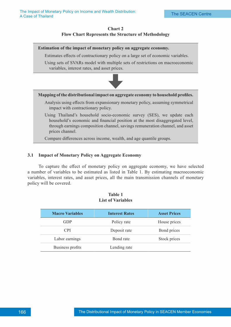
The methodology used in this analysis is based mainly on Casiraghi et al. (2017), which can be roughly divided into two parts; the impact of monetary policy on the aggregate economy and the mapping of the distributional impact on aggregate economy to household profiles (Chart 2). However, different from Casiraghi et al. (2017) who estimates multiple sets of single equations for the Bank of Italy quarterly model of the Italian economy (BIQM), our analysis is based on the estimation of a Structural Vector Autoregressions (SVARs) analysis for the aggregate economy.


A Case of Thailand

Chart 2Flow Chart Represents the Structure of Methodology

Estimation of the impact of monetary policy on aggregate economy.

Estimates effects of contractionary policy on a large set of economic variables.Using sets of SVARs model with multiple sets of restrictions on macroeconomic

variables, interest rates, and asset prices.

Mapping of the distributional impact on aggregate economy to household profiles.

Analysis using effects from expansionary monetary policy, assuming symmetrical impact with contractionary policy.

Using Thailand’s household socio-economic survey (SES), we update each household’s economic and financial position at the most disaggregated level, through earnings composition channel, savings remuneration channel, and asset prices channel.

Compare differences across income, wealth, and age quantile groups.

3.1 Impact of Monetary Policy on Aggregate Economy

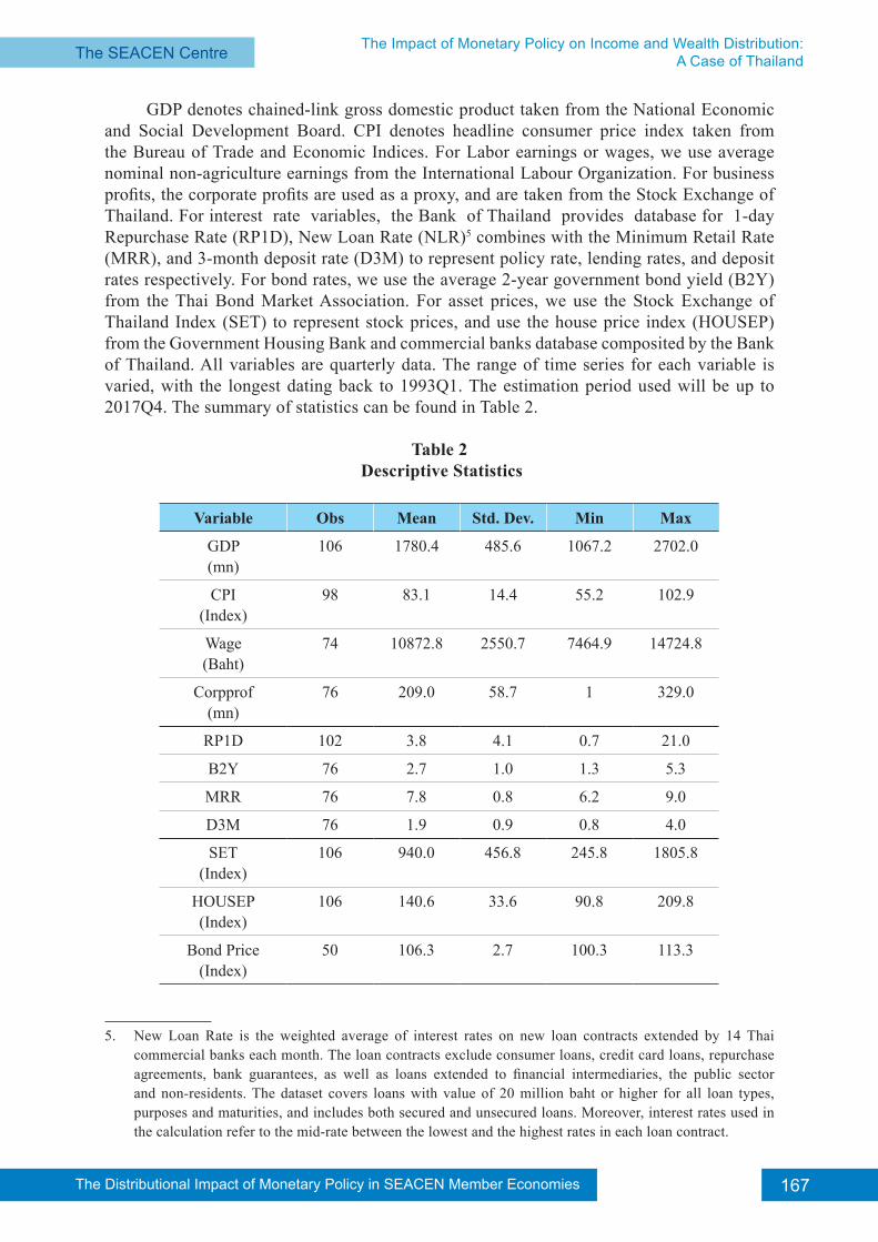
To capture the effect of monetary policy on aggregate economy, we have selected a number of variables to be estimated as listed in Table 1. By estimating macroeconomic variables, interest rates, and asset prices, all the main transmission channels of monetary policy will be covered.

Table 1List of Variables

Macro Variables Interest Rates Asset Prices

GDP Policy rate House prices

CPI Deposit rate Bond prices

Labor earnings Bond rate Stock prices

Business profits Lending rate


A Case of Thailand

GDP denotes chained-link gross domestic product taken from the National Economic and Social Development Board. CPI denotes headline consumer price index taken from the Bureau of Trade and Economic Indices. For Labor earnings or wages, we use average nominal non-agriculture earnings from the International Labour Organization. For business profits, the corporate profits are used as a proxy, and are taken from the Stock Exchange of Thailand. For interest rate variables, the Bank of Thailand provides database for 1-day Repurchase Rate (RP1D), New Loan Rate (NLR)5 combines with the Minimum Retail Rate (MRR), and 3-month deposit rate (D3M) to represent policy rate, lending rates, and deposit rates respectively. For bond rates, we use the average 2-year government bond yield (B2Y) from the Thai Bond Market Association. For asset prices, we use the Stock Exchange of Thailand Index (SET) to represent stock prices, and use the house price index (HOUSEP) from the Government Housing Bank and commercial banks database composited by the Bank of Thailand. All variables are quarterly data. The range of time series for each variable is varied, with the longest dating back to 1993Q1. The estimation period used will be up to 2017Q4. The summary of statistics can be found in Table 2.

Table 2 Descriptive Statistics

Variable Obs Mean Std. Dev. Min Max

GDP (mn)

106 1780.4 485.6 1067.2 2702.0

CPI (Index)

98 83.1 14.4 55.2 102.9

Wage (Baht)

74 10872.8 2550.7 7464.9 14724.8

Corpprof(mn)

76 209.0 58.7 1 329.0

RP1D 102 3.8 4.1 0.7 21.0

B2Y 76 2.7 1.0 1.3 5.3

MRR 76 7.8 0.8 6.2 9.0

D3M 76 1.9 0.9 0.8 4.0

SET (Index)

106 940.0 456.8 245.8 1805.8

HOUSEP(Index)

106 140.6 33.6 90.8 209.8

Bond Price(Index)

50 106.3 2.7 100.3 113.3

5. New Loan Rate is the weighted average of interest rates on new loan contracts extended by 14 Thai commercial banks each month. The loan contracts exclude consumer loans, credit card loans, repurchase agreements, bank guarantees, as well as loans extended to financial intermediaries, the public sector and non-residents. The dataset covers loans with value of 20 million baht or higher for all loan types, purposes and maturities, and includes both secured and unsecured loans. Moreover, interest rates used in the calculation refer to the mid-rate between the lowest and the highest rates in each loan contract.


A Case of Thailand

3.2 Mapping of the Distributed Impact to Household Profiles

The results from the SVAR model are then mapped onto household-level data, assuming a symmetric impact between contractionary and expansionary monetary policy. We make every effort to update all related items. However, due to the lack of some information, several assumptions are made through the mapping process. Three transmission channels will be considered in this study: earnings composition, savings remuneration and asset price channels. According to Casiraghi et al. (2017), these channels can be summarized respectively by the equations below.

(1)

(2)

(3)

(4)

From the earnings composition in (1), the main sources of income are considered. Households mostly receive wages as their main income, while those who are self-employed rely on business profits. Thus, non-financial income (YNi,t) is composed of labor earnings or wages (YLi,t), business profits (πi,t), and other income such as transfers (AYi,t). From savings remuneration in (2), interest income and payments are considered. This financial income (YFi.t) is composed of interest received from deposit rate (rd,t) times amount of deposits (Di,t-1), interest received from bond yield (rb,t) times amount of bond holding (Bi,t-1), and other financial income (AFYi.t), but deducted by interest paid from lending rate (rl,t) times amount of loans (Li,t-1). Finally, for asset prices in (3), it considers the value of asset holdings from the wealth perspective. The amount of gross wealth (GWi,t) is composed of house price (Ph,t) times number of house holding (Hi,t), bond price (Pb,t) times amount of bond holding, stock price (Pa,t) times amount of stock holding (Ai,t), and amount of deposit. However, these holdings of assets might not come from income alone, but can also come from borrowings. Thus, to consider net wealth (Wi,t), gross wealth has to be deducted by the amount of loans as in (4).


A Case of Thailand

3.2.1 Earnings Composition Channel

Based on equation (1), only three components of household non-financial income, labor earnings, business profits and transfers, are allowed to respond to a change in the policy rate. Labor earnings are regarded as the main source of income for the majority of Thai households, according to the household socio-economic survey. As a number of studies show that labor earnings are not only determined by macroeconomic variables, but also by the characteristics of workers, we construct an auxiliary equation to estimate the effects of monetary policy in order to control for such factors. A further explanation of the construction and estimation of the auxiliary equation will be given in Section 5. Apart from labor earnings, it appears that the sum of business profits is large amongst high-income households whilst low-income ones rely heavily on transfers. However, the impacts on transfers are ignored as we firmly believe that it would depend on fiscal policy rather than monetary policy.

3.2.2 Savings Remunerations Channel

Interest receipts and payments pertaining to the informal financial sector are excluded from the analysis because we do not know whether or not non-bank lenders adjust their lending rates in accordance with the policy rate. Due to the absence of information about the interest rates at the household level, it is presumed that banks offer the same deposit and lending rates to households, and all rates are adjustable with regard to the policy rate.

3.2.3 Asset Price Channel

By the supposition that a change in policy rate affects only house and stock prices, the outstanding values of other assets such as savings and bonds remain constant throughout the analysis. However, since we are unable to disaggregate bond and equity, the ratio of bond to equity, which equals to 40:60, is applied to all households. The figure is obtained from the Flow of Funds Accounts published by the National Economic and Social Development Council (NESDC) in 2017 where data on bond and equity owned by households are reported at the national level. Apart from that, it is also assumed that there is no shift in the composition of household assets after the policy rate changes, e.g. if the policy rate falls, stock prices will increase, but households will not sell stocks to buy a new house.

Micro data from the Household Socio-economic Survey (SES) administered by the National Statistical Office (NSO) are taken to estimate the distributional impact of monetary policy. The full dataset containing all information on household income, expenditure and wealth is released once every alternate year. This study uses the most recent observations which were released in 2017. Aside from the aforementioned, the SES also provides details of family compositions that allows us to scrutinize various aspects of the effects of monetary policy.


A Case of Thailand

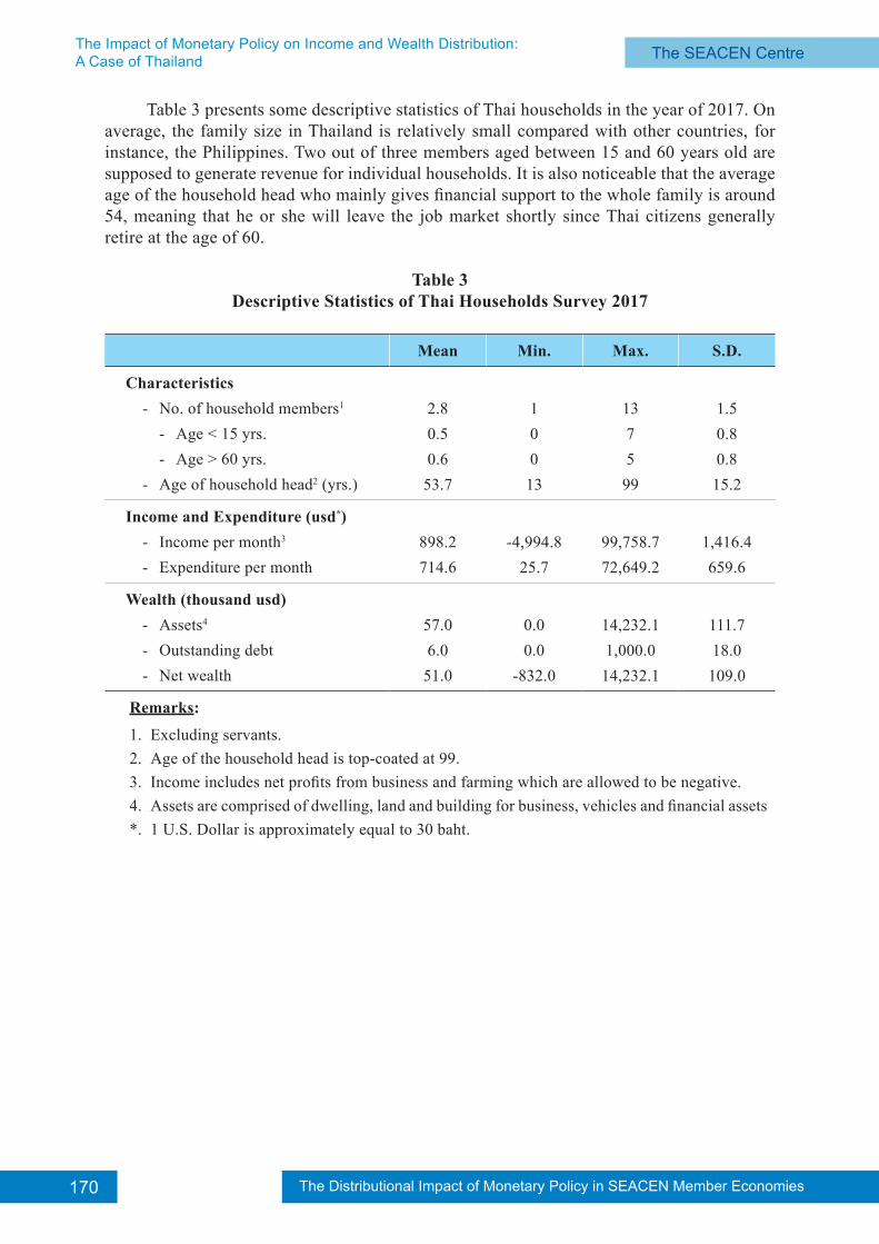
Table 3 presents some descriptive statistics of Thai households in the year of 2017. On average, the family size in Thailand is relatively small compared with other countries, for instance, the Philippines. Two out of three members aged between 15 and 60 years old are supposed to generate revenue for individual households. It is also noticeable that the average age of the household head who mainly gives financial support to the whole family is around 54, meaning that he or she will leave the job market shortly since Thai citizens generally retire at the age of 60.

Table 3Descriptive Statistics of Thai Households Survey 2017

Mean Min. Max. S.D.

Characteristics- No. of household members1

- Age < 15 yrs.- Age > 60 yrs.

- Age of household head2 (yrs.)

2.80.50.6

53.7

100

13

1375

99

1.50.80.8

15.2

Income and Expenditure (usd*)- Income per month3

- Expenditure per month898.2714.6

-4,994.825.7

99,758.772,649.2

1,416.4659.6

Wealth (thousand usd)- Assets4

- Outstanding debt- Net wealth

57.06.0

51.0

0.00.0

-832.0

14,232.11,000.0

14,232.1

111.718.0

109.0

Remarks:

1. Excluding servants.2. Age of the household head is top-coated at 99.3. Income includes net profits from business and farming which are allowed to be negative.4. Assets are comprised of dwelling, land and building for business, vehicles and financial assets*. 1 U.S. Dollar is approximately equal to 30 baht.

171The Distributional Impact of Monetary Policy in SEACEN Member Economies The SEACEN Centre The SEACEN Centre The Impact of Monetary Policy on Income and Wealth Distribution:

A Case of Thailand

Regarding household income and expenditure, it is found that the minimum of earnings is negative whilst the lowest expense is greater than zero. This indicates that some households make a loss from running a business or farming during the year but have to spend some money to maintain their livelihood. Likewise, the wealth statistics show that some households do not have any assets but take out loans. By taking these two numerical facts into consideration, it can be conjectured that a number of Thai households need to borrow money to finance consumption.

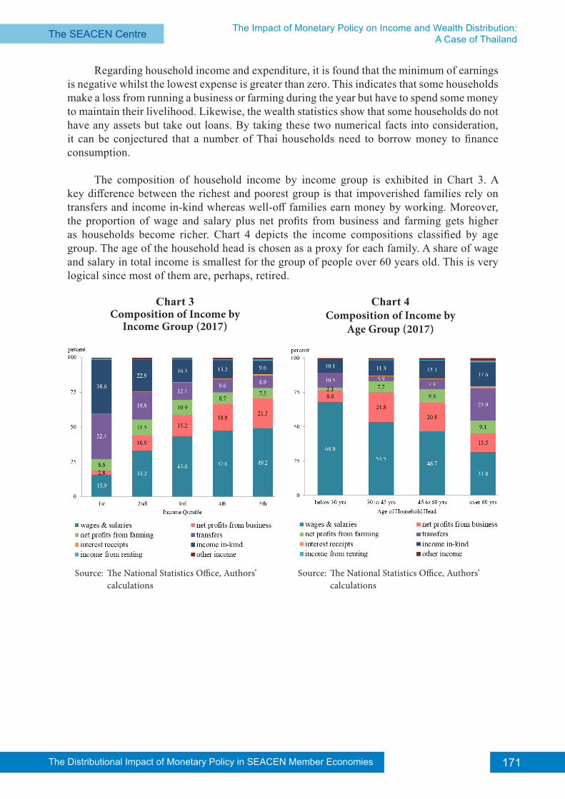
The composition of household income by income group is exhibited in Chart 3. A key difference between the richest and poorest group is that impoverished families rely on transfers and income in-kind whereas well-off families earn money by working. Moreover, the proportion of wage and salary plus net profits from business and farming gets higher as households become richer. Chart 4 depicts the income compositions classified by age group. The age of the household head is chosen as a proxy for each family. A share of wage and salary in total income is smallest for the group of people over 60 years old. This is very logical since most of them are, perhaps, retired.

Chart 3Composition of Income by

Income Group (2017)

Chart 4Composition of Income by

Age Group (2017)

Source: The National Statistics Office, Authors’ calculations



A Case of Thailand

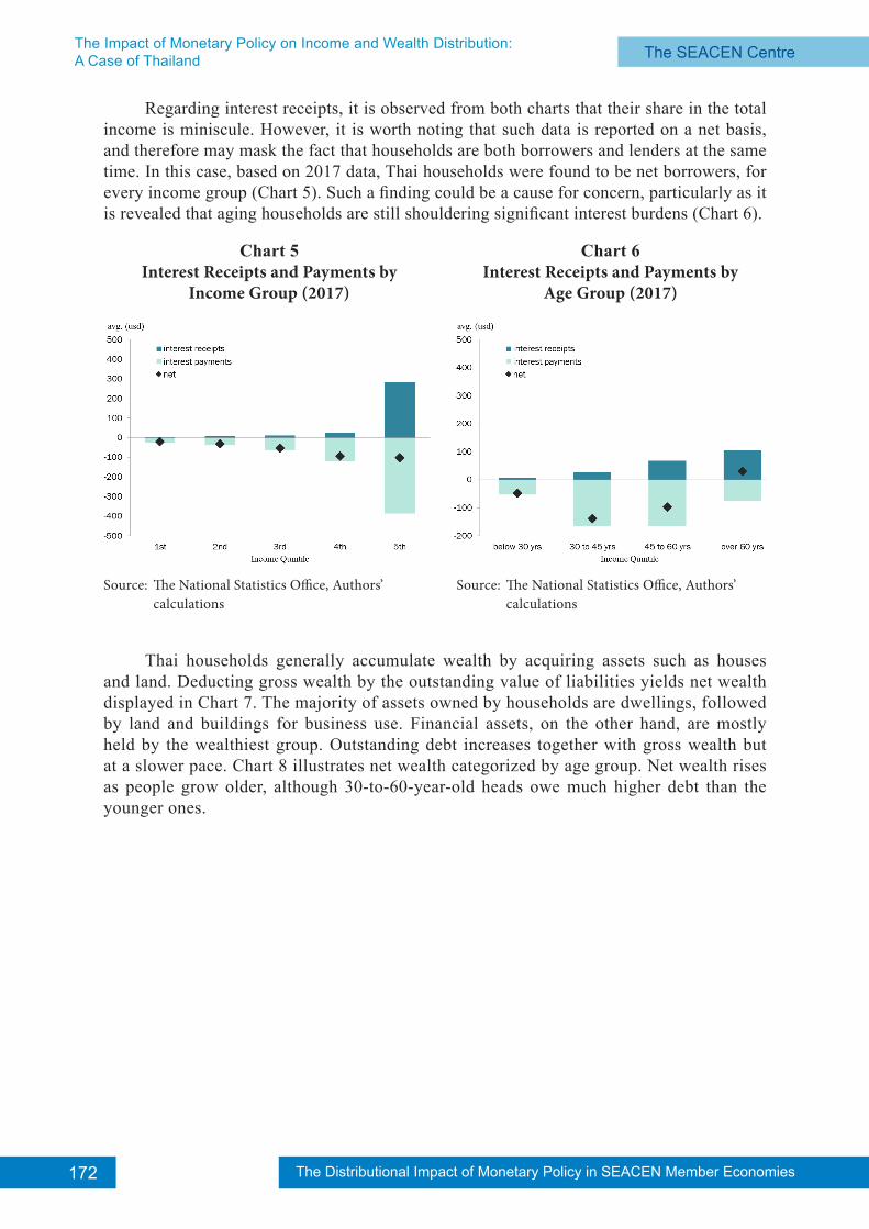
Regarding interest receipts, it is observed from both charts that their share in the total income is miniscule. However, it is worth noting that such data is reported on a net basis, and therefore may mask the fact that households are both borrowers and lenders at the same time. In this case, based on 2017 data, Thai households were found to be net borrowers, for every income group (Chart 5). Such a finding could be a cause for concern, particularly as it is revealed that aging households are still shouldering significant interest burdens (Chart 6).

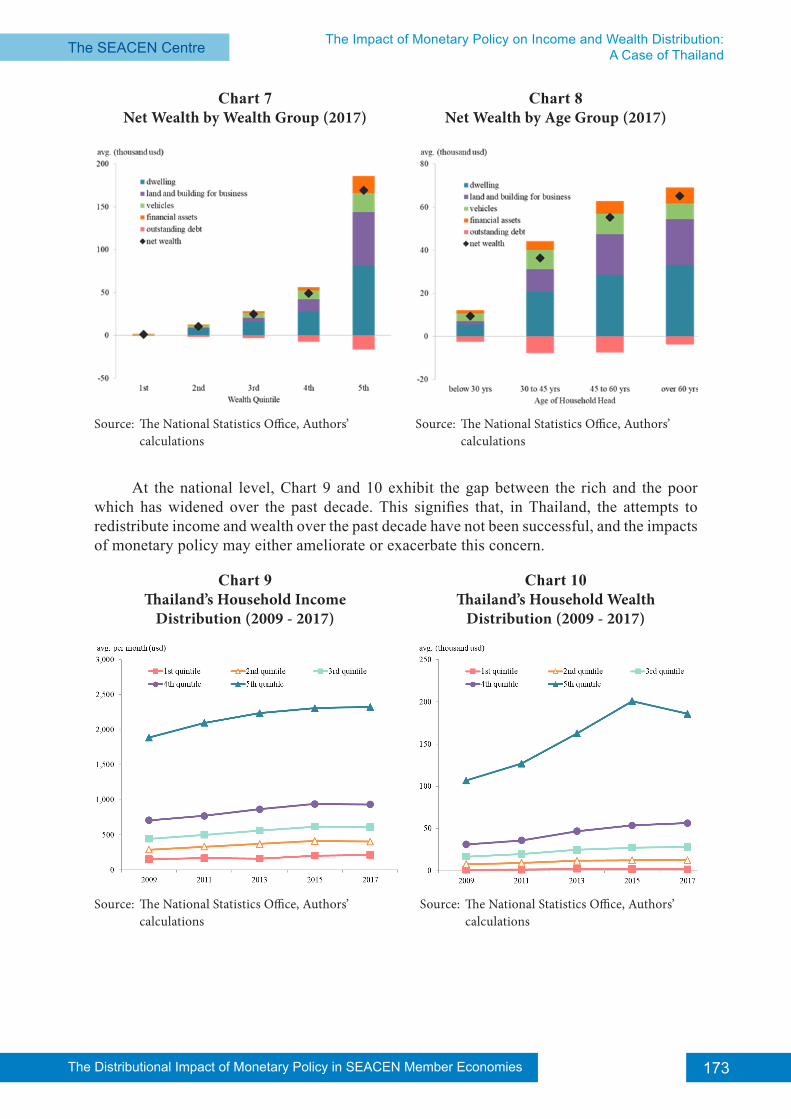
Thai households generally accumulate wealth by acquiring assets such as houses

and land. Deducting gross wealth by the outstanding value of liabilities yields net wealth displayed in Chart 7. The majority of assets owned by households are dwellings, followed by land and buildings for business use. Financial assets, on the other hand, are mostly held by the wealthiest group. Outstanding debt increases together with gross wealth but at a slower pace. Chart 8 illustrates net wealth categorized by age group. Net wealth rises as people grow older, although 30-to-60-year-old heads owe much higher debt than the younger ones.

Chart 5Interest Receipts and Payments by

Income Group (2017)

Chart 6Interest Receipts and Payments by

Age Group (2017)




A Case of Thailand

At the national level, Chart 9 and 10 exhibit the gap between the rich and the poor which has widened over the past decade. This signifies that, in Thailand, the attempts to redistribute income and wealth over the past decade have not been successful, and the impacts of monetary policy may either ameliorate or exacerbate this concern.

Chart 7Net Wealth by Wealth Group (2017)

Chart 8Net Wealth by Age Group (2017)



Chart 10 Thailand’s Household Wealth

Distribution (2009 - 2017)

Chart 9Thailand’s Household Income

Distribution (2009 - 2017)




A Case of Thailand

4. Analysis of Monetary Policy Impact on Aggregate Economy

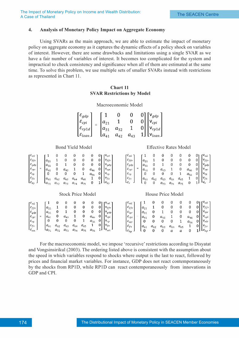
Using SVARs as the main approach, we are able to estimate the impact of monetary policy on aggregate economy as it captures the dynamic effects of a policy shock on variables of interest. However, there are some drawbacks and limitations using a single SVAR as we have a fair number of variables of interest. It becomes too complicated for the system and impractical to check consistency and significance when all of them are estimated at the same time. To solve this problem, we use multiple sets of smaller SVARs instead with restrictions as represented in Chart 11.

Chart 11 SVAR Restrictions by Model

Macroeconomic Model

Bond Yield Model Effective Rates Model

Stock Price Model House Price Model

For the macroeconomic model, we impose ‘recursive’ restrictions according to Disyatat and Vongsinsirikul (2003). The ordering listed above is consistent with the assumption about the speed in which variables respond to shocks where output is the last to react, followed by prices and financial market variables. For instance, GDP does not react contemporaneously by the shocks from RP1D, while RP1D can react contemporaneously from innovations in GDP and CPI.


A Case of Thailand

To address the ‘prize puzzle’ problem6, as is the case in Disyatat and Vongsinsirikul (2003), we include the bank loans variable (LOAN), which are credits to the non-financial sector from the Bank for International Settlements, into the model as well. However, an adjustment is made by replacing exogenous variables to inflation expectation (INFEXP) taken from Consensus Forecasts, instead of using exchange rate. This is in line with the regime change from exchange rate targeting, thus the use of exchange rate as an exogenous variable in Disyatat and Vongsinsirikul (2003), to flexible inflation targeting regime in the present day.

For remaining models, we impose ‘non-recursive’ restrictions based mainly from Elbourne (2007), with some adjustments made to fit with our analysis. Here, commodity prices, fed funds rates (FFR), and exchange rate are added to the system. This is because the remaining variables of interest for interest rates and asset prices channel are sometimes linked to and caused by factors other than macroeconomic fundamentals. Furthermore, Thailand’s characteristic as a small and open economy makes it susceptible to the external environment. Thus, a recursive structure used in prior models would not be appropriate for estimation, and we need to take into account a wider range of factors in the system. Inflation expectation (INFEXP) is also included as an exogenous variable to represent the inflation targeting regime. Note that in our analysis, money demand is dropped from the system as its importance diminishes over time and its inclusion failed the LR tests. We use Dubai oil price (DUBAI) to represent commodity prices, and USDTHB (FX) for the exchange rate. The ordering of each model is listed as Chart 11, where the variables of interest are ordered last.

For the stock price model, we restrict the system based on Zare et al. (2013). The SET index that represents stock prices is sensitive to shocks that occur in the economy and is swift to respond. Therefore, it is contemporaneously affected by shocks from every other variable in the system. For the bond yield model, similar restrictions are imposed. But only the exchange rate does not contemporaneously affect the bond yield, as the relationship between them is vague in Thailand. For the effective rates model, three variables are used in the same restrictions, namely NLR, MRR, and D3M. We run the model for each of these variables separately. The restrictions omit the contemporaneous effects from the external environment, namely DUBAI, FFR, and FX, as these variables mainly rely on bank decisions. Finally, for the house price model, a few adjustments are needed as the housing market behaves uniquely compared to other variables. We replace GDP with gross fixed capital formation (IPR) as it correlates more with house price7, and NLR is used as a proxy for policy rates. The model using NLR works because house prices are more sensitive to lending rates as it drives the demand for mortgages, and NLR tracks the movement of central bank’s policy actions quite closely.

6. In Disyatat and Vongsinsirikul (2003), price puzzles arise when a contractionary policy shock leads to a rise in inflation. An explanation is that policy makers might be able to observe variables that contain information about the future inflation, but they are left out of the model. Then a rise in policy rates might be associated with higher prices because they reflect policy responses to information indicating future inflation. To address this issue in the case of Thailand, bank credit is included in the system as the supply of bank loans is crucial for business investment in Thailand. Inclusion of bank loans helps because GDP and prices respond positively to innovations in bank lending.

7. We have tried replacing GDP with private consumption, as is used in a number of literatures, but the model failed the LR tests and house price did not appear significant in response to shocks of policy rate or lending rates.


A Case of Thailand

Preparing for SVARs, we ran the unit root test and cointegration test. We found that GDP, CPI, DUBAI, FX, SET, HOUSEP, and LOAN contain unit roots but are cointegrated. Therefore, we use the log transformation on these variables, while leaving the remaining interest rate variables unchanged.

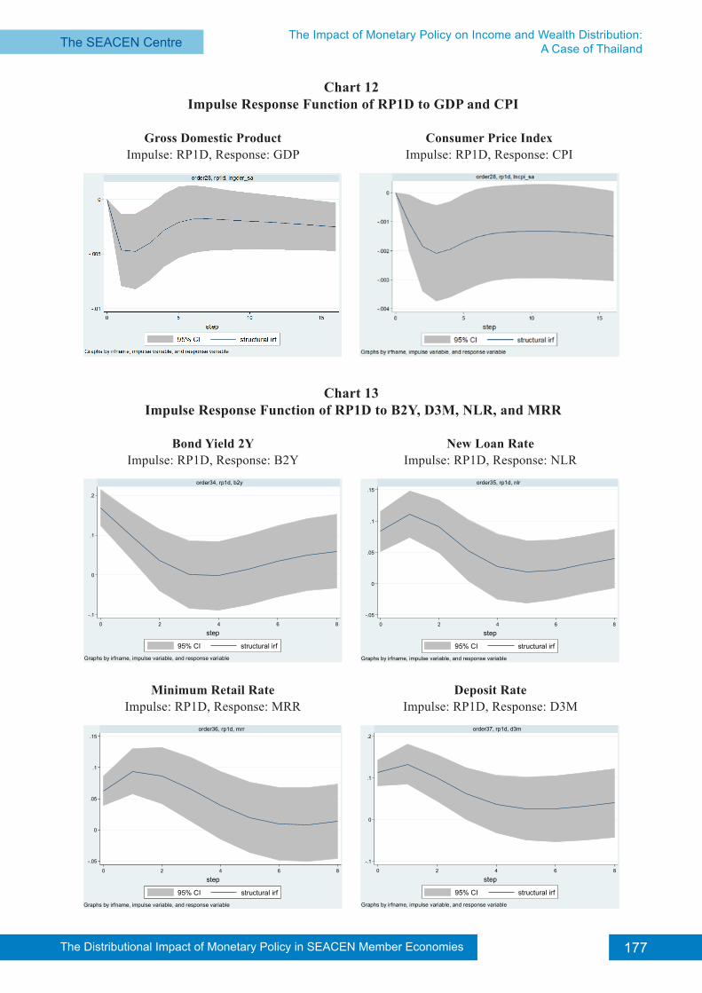
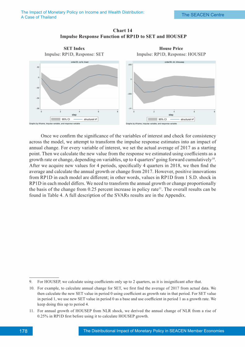
In order to derive the impact of monetary policy on the aggregate economy from SVARs, the impulse response analysis is the key to quantify it. We mainly focus the impulse from RP1D to the response of the variables of interest based on corresponding models explained in the previous section. Starting with the macroeconomic model, the impulse-responses of RP1D to GDP and CPI are shown in Chart 12. The positive shocks from RP1D to GDP and CPI are significant for 8 quarters before reverting to mean. It also has a negative impact on them, which is consistent with theories where contractionary monetary policy leads to a reduction in output and prices through the good and services market and money market. For other macroeconomic variables, we have also tried to add wages and corporate profits into the recursive structure and experimented with different ordering, but to no avail as they are both insignificant. However, the impact on wages will be explained in later sections. For the bond yield and effective rates model, the impulse-responses of RP1D to B2Y, D3M, NLR, and MRR are shown in Chart 13. The positive shocks from RP1D to effective rates and yields are positively significant as expected. The rise in policy rate should drive other corresponding interest rates to rise as well. However, unlike macroeconomic variables, it is significant for only around 3 quarters as they are susceptible to other factors and quick to respond. Finally, for the asset prices model, the impulse-responses of RP1D to SET and HOUSEP are shown in Chart 148. However, different behavior of stock price and house price can be observed. Stock price responds negatively for 2 quarters directly from the shock of the policy rate. On the other hand, house price initially does not respond to RP1D as it is insignificant. But as mentioned above, the replacement with NLR shock as a proxy causes HOUSEP to be significant for 2 quarters. Despite the difference in behavior, they are in line with the theory as rising interest rates drive down the value of the asset prices.

8. We have also tried estimating the impact from the shock of policy rates on bond prices. But the data for bond prices are limited and it is difficult to find a reliable benchmark. The results are also insignificant.


A Case of Thailand

Chart 12 Impulse Response Function of RP1D to GDP and CPI

Chart 13 Impulse Response Function of RP1D to B2Y, D3M, NLR, and MRR

Consumer Price IndexImpulse: RP1D, Response: CPI

Gross Domestic ProductImpulse: RP1D, Response: GDP

-.05

0

.05

.1

.15

0 2 4 6 8

order36, rp1d, mrr

95% CI structural irf

step

Graphs by irfname, impulse variable, and response variable

New Loan RateImpulse: RP1D, Response: NLR

Bond Yield 2YImpulse: RP1D, Response: B2Y

-.1

0

.1

.2

0 2 4 6 8

order34, rp1d, b2y


step


-.05

0

.05

.1

.15

0 2 4 6 8

order35, rp1d, nlr


step


Deposit RateImpulse: RP1D, Response: D3M

Minimum Retail RateImpulse: RP1D, Response: MRR

-.1

0

.1

.2

0 2 4 6 8

order37, rp1d, d3m


step



A Case of Thailand

Chart 14 Impulse Response Function of RP1D to SET and HOUSEP

Once we confirm the significance of the variables of interest and check for consistency

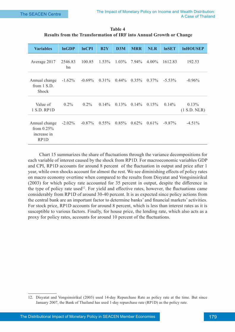
across the model, we attempt to transform the impulse response estimates into an impact of annual change. For every variable of interest, we set the actual average of 2017 as a starting point. Then we calculate the new value from the response we estimated using coefficients as a growth rate or change, depending on variables, up to 4 quarters9 going forward cumulatively10. After we acquire new values for 4 periods, specifically 4 quarters in 2018, we then find the average and calculate the annual growth or change from 2017. However, positive innovations from RP1D in each model are different; in other words, values in RP1D from 1 S.D. shock in RP1D in each model differs. We need to transform the annual growth or change proportionally the basis of the change from 0.25 percent increase in policy rate11. The overall results can be found in Table 4. A full description of the SVARs results are in the Appendix.

9. For HOUSEP, we calculate using coefficients only up to 2 quarters, as it is insignificant after that.10. For example, to calculate annual change for SET, we first find the average of 2017 from actual data. We

then calculate the new SET value in period 0 using coefficient as growth rate in that period. For SET value in period 1, we use new SET value in period 0 as a base and use coefficient in period 1 as a growth rate. We keep doing this up to period 4.

11. For annual growth of HOUSEP from NLR shock, we derived the annual change of NLR from a rise of 0.25% in RP1D first before using it to calculate HOUSEP growth.

-.01

-.005

0

.005

0 2 4 6 8

order38, nlr, lnhousep


step


House PriceImpulse: RP1D, Response: HOUSEP

SET IndexImpulse: RP1D, Response: SET

-.06

-.04

-.02

0

.02

0 2 4 6 8

order33, rp1d, lnset


step



A Case of Thailand

Table 4 Results from the Transformation of IRF into Annual Growth or Change

Variables lnGDP lnCPI B2Y D3M MRR NLR lnSET lnHOUSEP

Average 2017 2546.83bn

100.85 1.53% 1.03% 7.94% 4.00% 1612.83 192.53

Annual change from 1 S.D.

Shock

-1.62% -0.69% 0.31% 0.44% 0.35% 0.37% -5.53% -0.96%

Value of 1 S.D. RP1D

0.2% 0.2% 0.14% 0.13% 0.14% 0.15% 0.14% 0.13%(1 S.D. NLR)

Annual change from 0.25% increase in

RP1D

-2.02% -0.87% 0.55% 0.85% 0.62% 0.61% -9.87% -4.51%

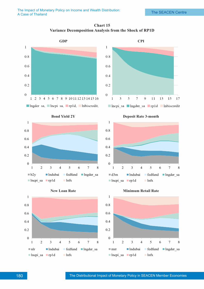
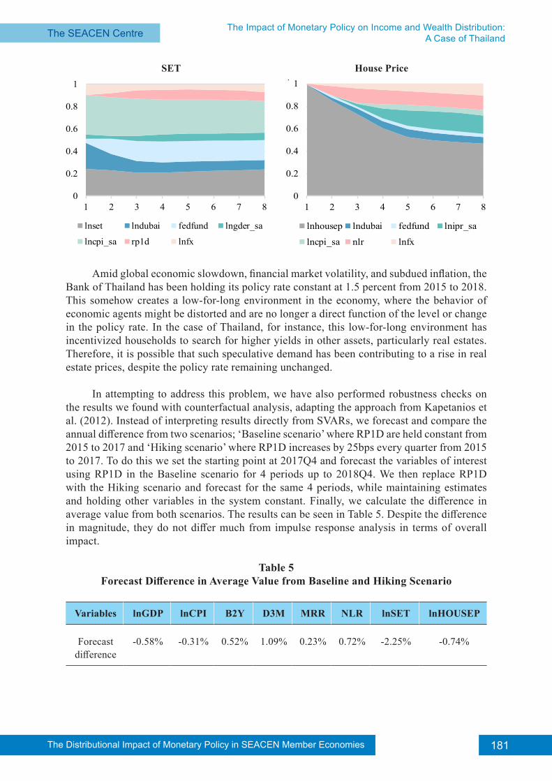
Chart 15 summarizes the share of fluctuations through the variance decompositions for each variable of interest caused by the shock from RP1D. For macroeconomic variables GDP and CPI, RP1D accounts for around 8 percent of the fluctuation in output and price after 1 year, while own shocks account for almost the rest. We see diminishing effects of policy rates on macro economy overtime when compared to the results from Disyatat and Vongsinsirikul (2003) for which policy rate accounted for 35 percent in output, despite the difference in the type of policy rate used12. For yield and effective rates, however, the fluctuations came considerably from RP1D of around 30-40 percent. It is as expected since policy actions from the central bank are an important factor to determine banks’ and financial markets’ activities. For stock price, RP1D accounts for around 8 percent, which is less than interest rates as it is susceptible to various factors. Finally, for house price, the lending rate, which also acts as a proxy for policy rates, accounts for around 10 percent of the fluctuations.

12. Disyatat and Vongsinsirikul (2003) used 14-day Repurchase Rate as policy rate at the time. But since January 2007, the Bank of Thailand has used 1-day repurchase rate (RP1D) as the policy rate.


A Case of Thailand

0

0.2

0.4

0.6

0.8

1

1 2 3 4 5 6 7 8

New Loan Rate

nlr lndubai fedfund lngder_sa

lncpi_sa rp1d lnfx

0

0.2

0.4

0.6

0.8

1

1 2 3 4 5 6 7 8

Deposit Rate 3-month

d3m lndubai fedfund lngder_sa

lncpi_sa rp1d lnfx

0

0.2

0.4

0.6

0.8

1

1 2 3 4 5 6 7 8

Bond Yield 2Y

b2y lndubai fedfund lngder_sa

lncpi_sa rp1d lnfx

Chart 15Variance Decomposition Analysis from the Shock of RP1D

0

0.2

0.4

0.6

0.8

1

1 2 3 4 5 6 7 8

Minimum Retail Rate

mrr lndubai fedfund lngder_sa

lncpi_sa rp1d lnfx

CPIGDP

Deposit Rate 3-monthBond Yield 2Y

Minimum Retail RateNew Loan Rate


A Case of Thailand

0

0.2

0.4

0.6

0.8

1

1 2 3 4 5 6 7 8

SET

lnset lndubai fedfund lngder_sa

lncpi_sa rp1d lnfx

Amid global economic slowdown, financial market volatility, and subdued inflation, the Bank of Thailand has been holding its policy rate constant at 1.5 percent from 2015 to 2018. This somehow creates a low-for-long environment in the economy, where the behavior of economic agents might be distorted and are no longer a direct function of the level or change in the policy rate. In the case of Thailand, for instance, this low-for-long environment has incentivized households to search for higher yields in other assets, particularly real estates. Therefore, it is possible that such speculative demand has been contributing to a rise in real estate prices, despite the policy rate remaining unchanged.

In attempting to address this problem, we have also performed robustness checks on the results we found with counterfactual analysis, adapting the approach from Kapetanios et al. (2012). Instead of interpreting results directly from SVARs, we forecast and compare the annual difference from two scenarios; ‘Baseline scenario’ where RP1D are held constant from 2015 to 2017 and ‘Hiking scenario’ where RP1D increases by 25bps every quarter from 2015 to 2017. To do this we set the starting point at 2017Q4 and forecast the variables of interest using RP1D in the Baseline scenario for 4 periods up to 2018Q4. We then replace RP1D with the Hiking scenario and forecast for the same 4 periods, while maintaining estimates and holding other variables in the system constant. Finally, we calculate the difference in average value from both scenarios. The results can be seen in Table 5. Despite the difference in magnitude, they do not differ much from impulse response analysis in terms of overall impact.

Table 5Forecast Difference in Average Value from Baseline and Hiking Scenario

Variables lnGDP lnCPI B2Y D3M MRR NLR lnSET lnHOUSEP

Forecast difference

-0.58% -0.31% 0.52% 1.09% 0.23% 0.72% -2.25% -0.74%

0

0.2

0.4

0.6

0.8

1

1 2 3 4 5 6 7 8

House Price

lnhousep lndubai fedfund lnipr_sa

lncpi_sa nlr lnfx

House PriceSET


A Case of Thailand

5. Analysis of the Distributed Monetary Policy Impact on Household Profiles

This study focuses merely on the employed. A change in the policy rate is assumed to exert no effect on the decision to enter or leave the workforce. The presence of heterogeneity in labor earnings has been widely discussed in literature. In the case of Thailand, for example, Warunsiri and McNown (2010) construct models to estimate the returns to education by taking unobserved heterogeneity into account. Such heterogeneity is often referred to the ability or motivation to work varied by the characteristics of workers. It is, therefore, useful to incorporate data from the Labour Force Survey (LFS), which is conducted by the NSO as well, into our estimation to control for individual-specific effects.

The NSO, in fact, collects data on wages and workers’ characteristics on a monthly basis. The data are, however, regarded as repeated cross-sections because the same respondents are not required to complete the survey every month, but even so, it is still able to create pseudo-panel data defined by geographical area, gender, marital status and the level of education. Five years of the survey, from 2013 to 2017, are used to obtain 1,224 clusters in total. After that, the following equation is estimated using fixed effect regression.

(5)

where indexes individual groups of workers, and indexes year. denotes monthly labour income in nominal terms which includes wage / salary, overtime pay and bonus.

denotes the average age of workers as a proxy of working experience. and denote real GDP and Consumer Price Index. denotes the percentage of

labor income share to GDP13

Real GDP and headline inflation are employed as linkages between the policy rate and wage. The labor income share to GDP is added to the equation above for two reasons. One is to measure the gap between wage and productivity. If labor income share to GDP rises, it implies wage paid to workers is greater than labor productivity per se, so the employer will cut down employment, and wage will eventually go down (Conway et al., 2015). The relationship between labor income share and wage is thus expected to be negative. The other one is that a decrease in labor income share to GDP implies an increase in capital share to GDP, given only two factors, labor and capital, are used in production. As automation has received growing attention, an increase in GDP may not induce employment but investment in machinery and equipment in lieu. Including such a variable is, therefore, supposed to capture this phenomenon and help reduce bias towards the coefficient of real GDP.

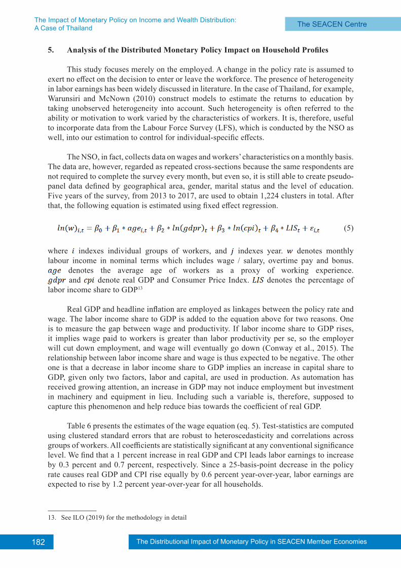
Table 6 presents the estimates of the wage equation (eq. 5). Test-statistics are computed using clustered standard errors that are robust to heteroscedasticity and correlations across groups of workers. All coefficients are statistically significant at any conventional significance level. We find that a 1 percent increase in real GDP and CPI leads labor earnings to increase by 0.3 percent and 0.7 percent, respectively. Since a 25-basis-point decrease in the policy rate causes real GDP and CPI rise equally by 0.6 percent year-over-year, labor earnings are expected to rise by 1.2 percent year-over-year for all households.

13. See ILO (2019) for the methodology in detail


A Case of Thailand

Table 6 Estimates of the Wage Equation

Dep. var. = ln (wage) Coefficient

age 0.016***

(0.002)

ln (gdpr) 0.292***

(0.043)

LIS -0.024***

(0.002)

ln (cpi) 0.707***

(0.196)

constant 4.015***

(0.957)

Adjusted R2

F-statistics0.19

163.23

Numbers in parentheses are clustered standard errors. *** indicates significance at 1% level.

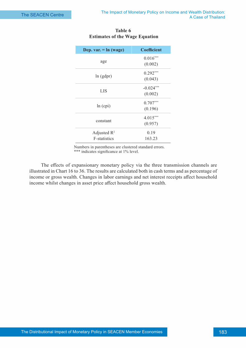
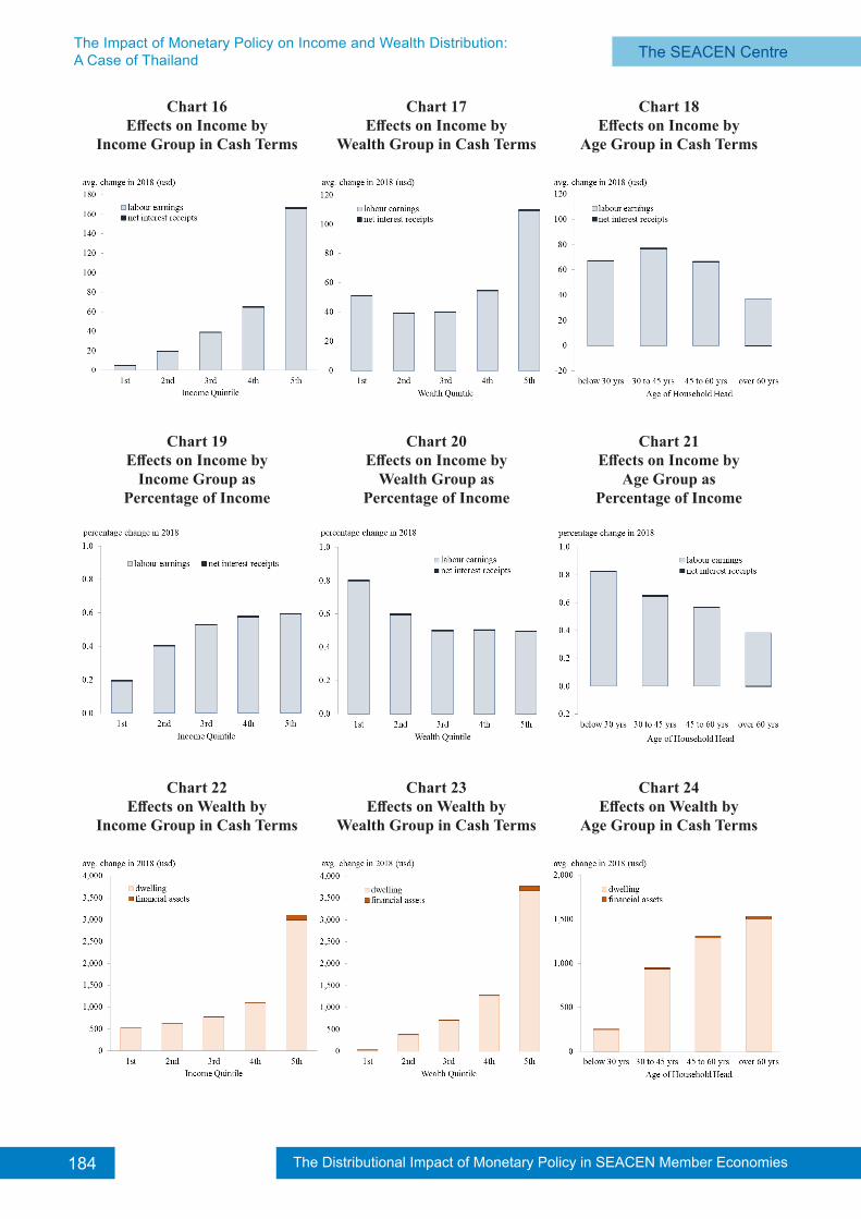
The effects of expansionary monetary policy via the three transmission channels are

illustrated in Chart 16 to 36. The results are calculated both in cash terms and as percentage of income or gross wealth. Changes in labor earnings and net interest receipts affect household income whilst changes in asset price affect household gross wealth.


A Case of Thailand

Chart 17Effects on Income by

Wealth Group in Cash Terms


Income Group in Cash Terms


Age Group in Cash Terms


Wealth Group asPercentage of Income


Income Group asPercentage of Income


Age Group asPercentage of Income

Chart 23Effects on Wealth by

Wealth Group in Cash Terms


Income Group in Cash Terms


Age Group in Cash Terms


A Case of Thailand


Wealth Group asPercentage of Wealth


Income Group asPercentage of Wealth


Age Group asPercentage of Wealth

Chart 29Effects on Income and

Wealth by Wealth Groupin Cash Terms


Wealth by Income Groupin Cash Terms

Chart 30Effects on Income andWealth by Age Group

in Cash Terms


Wealth by Wealth Group as Percentage Change of Income


Wealth by Income Group as Percentage Change of Income


Wealth by Age Group as Percentage Change of Income


A Case of Thailand

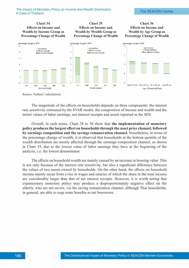
Source: Authors’ calculations.

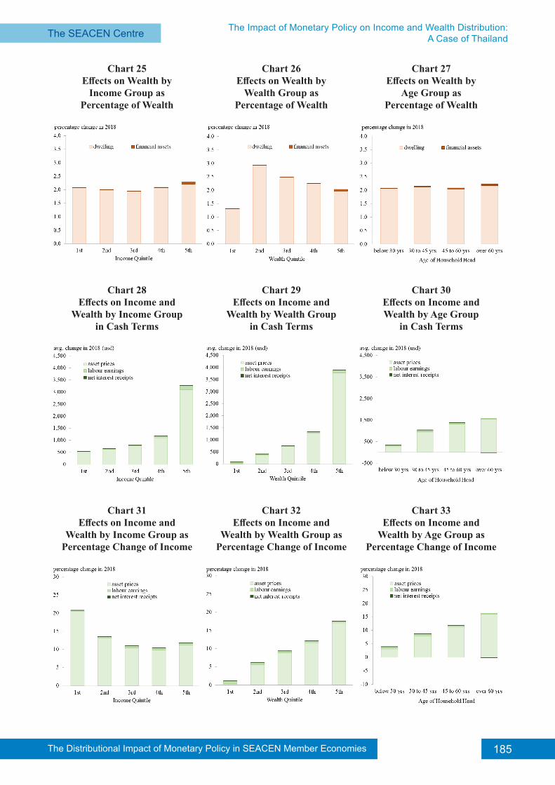
The magnitude of the effects on households depends on three components: the interest rate sensitivity estimated by the SVAR model, the composition of income and wealth and the initial values of labor earnings, net interest receipts and assets reported in the SES.

Overall, in cash terms, Chart 28 to 30 show that the implementation of monetary policy produces the largest effect on households through the asset price channel, followed by earnings composition and the savings remuneration channel. Nonetheless, in terms of the percentage change of wealth, it is observed that households at the bottom quintile of the wealth distribution are mostly affected through the earnings composition channel, as shown in Chart 35, due to the lowest value of labor earnings they have at the beginning of the analysis, i.e. the lowest denominator.

The effects on household wealth are mainly caused by an increase in housing value. This is not only because of the interest rate sensitivity, but also a significant difference between the values of two assets owned by households. On the other hand, the effects on household income mainly occur from a rise in wages and salaries of which the share in the total income are considerably larger than that of net interest receipts. However, it is worth noting that expansionary monetary policy may produce a disproportionately negative effect on the elderly, who are net savers, via the saving remuneration channel, although Thai households, in general, are able to reap some benefits as net borrowers.


Wealth by Wealth Group as Percentage Change of Wealth


Wealth by Income Group as Percentage Change of Wealth


Wealth by Age Group as Percentage Change of Wealth


A Case of Thailand

6. Discussion

Our empirical findings shed light on a low-for-long rate environment in Thailand. First, according to conventional macroeconomic frameworks, for instance, the Representative Agent New Keynesian (RANK), it is stated that the policy rate cut leads households to take out more consumer loans, hence causing aggregate consumption to increase. This is supported by Chuchurd (2006) and Suwanik and Peerawattanachart (2018) which demonstrate that the consumption of goods and services by poor households in Thailand can be increased by debt due to liquidity constraint. Nonetheless, since most of Thai households in our micro data are regarded as net borrowers, and at the country level, the ratio of household debt to GDP has remained high for several years, a further decrease in the policy rate might not be able to increase the country’s aggregate consumption. Second, although we find that the expansionary monetary policy has a positive effect on house prices, the magnitude of the effect may be exaggerated because of the artificial demand for housing that typically occurs when the policy rate has been low for a long horizon. These two arguments, therefore, suggest the use of conventional monetary policy tools such as the interest rate together with the imposing of macroprudential regulations and the undertaking of structural reforms to boost the sustainable economic growth.

Furthermore, there are some limitations to bear in mind when interpreting our results. First, we perform a partial equilibrium analysis to examine the effects of expansionary monetary policy in this study. Second, due to the lack of household panel survey data, the analysis only gives short-run impacts on households.

7. Conclusion and Policy Recommendation

Our analysis is based on estimating the distributional impact of monetary policy on individual households through the lens of income, wealth, and age distribution. By estimating multiple sets of SVARs, we do find the significance of Bank of Thailand’s policy rate on the aggregate economy, and financial markets. Thus, we are able to map these results onto Thailand’s Household Socio-Economic Survey. At the household level, it is found that wealthy households are more sensitive to monetary policy, compared with the poor ones, mostly through the asset price channel whilst the effects through savings remuneration are minimal. However, as we firmly believe that a change in transfers, which are supposed to tremendously affect income of poor households, depends heavily on fiscal policy, thus the use of a policy mix is recommended in order to reduce income and wealth inequality in Thailand. More importantly, such inequality should be a wake-up call for the government to focus on structural policies, particularly by expediting the much-needed investment in a social safety net and health infrastructure.


A Case of Thailand

References

Bunn, P.; A. Pugh and C. Yeates, (2018), “The Distributional Impact of Monetary Policy Easing in the UK between 2008 and 2014,” Bank of England Staff Working Paper, No. 720.

Casiraghi, M.; E. Gaiotti ; L. Rodano and A. Secchi, (2017), “A ‘Reverse Robin Hood’? The Distributional Implications of Non-standard Monetary Policy for Italian Households,” Journal of International Money and Finance, Vol.85.

Colciago, A.; A. Samarina and J. Haan, (2019), “Central Bank Policies and Income and Wealth Inequality: A Survey,” Journal of Economic Surveys, Vol.0

Chucherd, T., (2006), “The Effect of Household Debt on Consumption in Thailand,” Bank of Thailand Discussion Paper, No. 1/2006.

Conway, P.; L. Meehan and D. Parham, (2015), “Who Benefits from Productivity Growth? –The Labour Income Share in New Zealand,” New Zealand Productivity Commission, Working Paper, No. 2015/1. Wellington: Productivity Commission.

Disyatat, P. and P. Vongsinsirikul, (2003), “Monetary Policy and the Transmission Mechanism in Thailand,” Journal of Asian Economics, Vol.14.

Elbourne, A., (2007), “The UK Housing Market and the Monetary Policy Transmission Mechanism: An SVAR Approach,” Journal of Housing Economics, Vol.17.

International Labour Office, (ILO), (2019), The Global Labour Income Share and Distribution.

Kapetanios, G.; H. Mumtaz; I. Stevens and K. Theodoridis, (2012), “Assessing the Economy-wide Effects of Quantitative Easing,” Bank of England Staff Working Paper, No. 443.

Romer, C. and D. Romer, (1999), “Monetary Policy and the Well-being of the Poor,” Economic Review, Vol.17, No.1.

Suwanik, S. and K. Peerawattanachart, (2018), “Household Debt in SEACEN Economies: Thailand,” The SEACEN Centre, Chapter 7.

Warunsiri, S. and R. McNown, (2010), “The Returns to Education in Thailand: A Pseudo-Panel Approach,” World Development, Vol.38, No.11.

Zare, R.; M. Azali and M. S. Habibullahc, (2013), “The Reaction of Stock Prices to Monetary Policy Shocks in Malaysia: A Structural Vector Autoregressive Model,” International Organization for Research and Development.


A Case of Thailand

Appendix

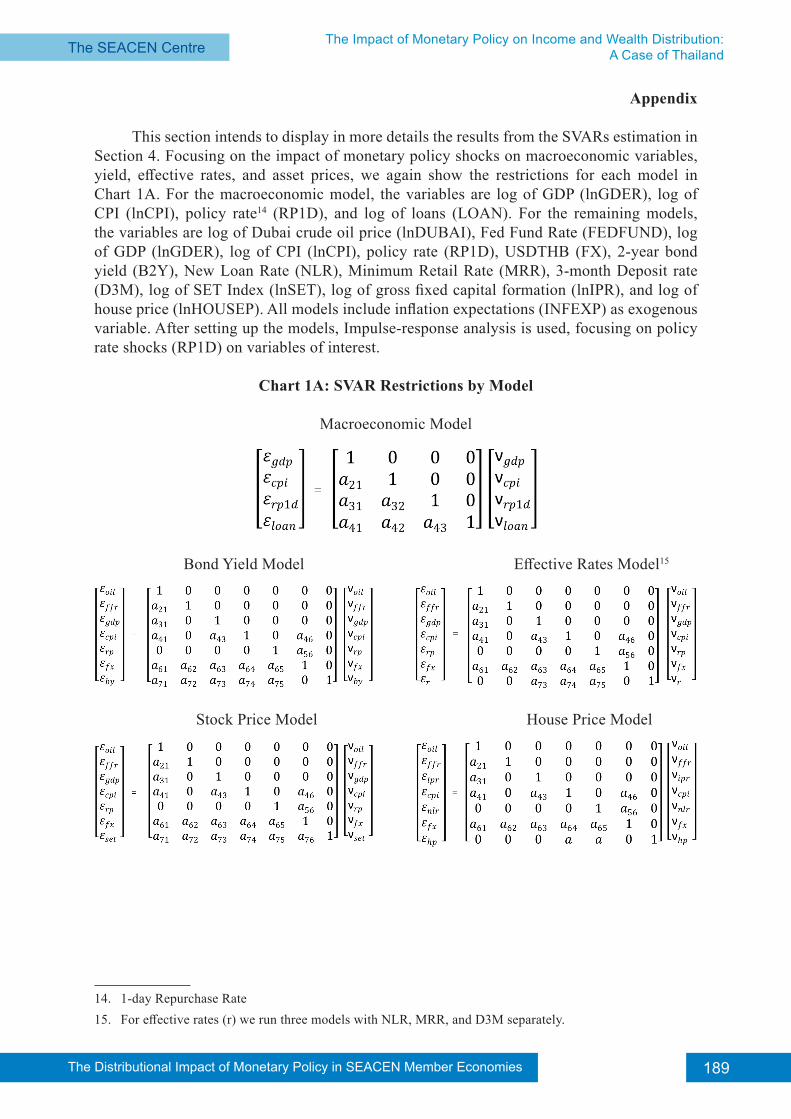
This section intends to display in more details the results from the SVARs estimation in Section 4. Focusing on the impact of monetary policy shocks on macroeconomic variables, yield, effective rates, and asset prices, we again show the restrictions for each model in Chart 1A. For the macroeconomic model, the variables are log of GDP (lnGDER), log of CPI (lnCPI), policy rate14 (RP1D), and log of loans (LOAN). For the remaining models, the variables are log of Dubai crude oil price (lnDUBAI), Fed Fund Rate (FEDFUND), log of GDP (lnGDER), log of CPI (lnCPI), policy rate (RP1D), USDTHB (FX), 2-year bond yield (B2Y), New Loan Rate (NLR), Minimum Retail Rate (MRR), 3-month Deposit rate (D3M), log of SET Index (lnSET), log of gross fixed capital formation (lnIPR), and log of house price (lnHOUSEP). All models include inflation expectations (INFEXP) as exogenous variable. After setting up the models, Impulse-response analysis is used, focusing on policy rate shocks (RP1D) on variables of interest.

Chart 1A: SVAR Restrictions by Model

Macroeconomic Model

Bond Yield Model Effective Rates Model15

Stock Price Model House Price Model

14. 1-day Repurchase Rate15. For effective rates (r) we run three models with NLR, MRR, and D3M separately.


A Case of Thailand

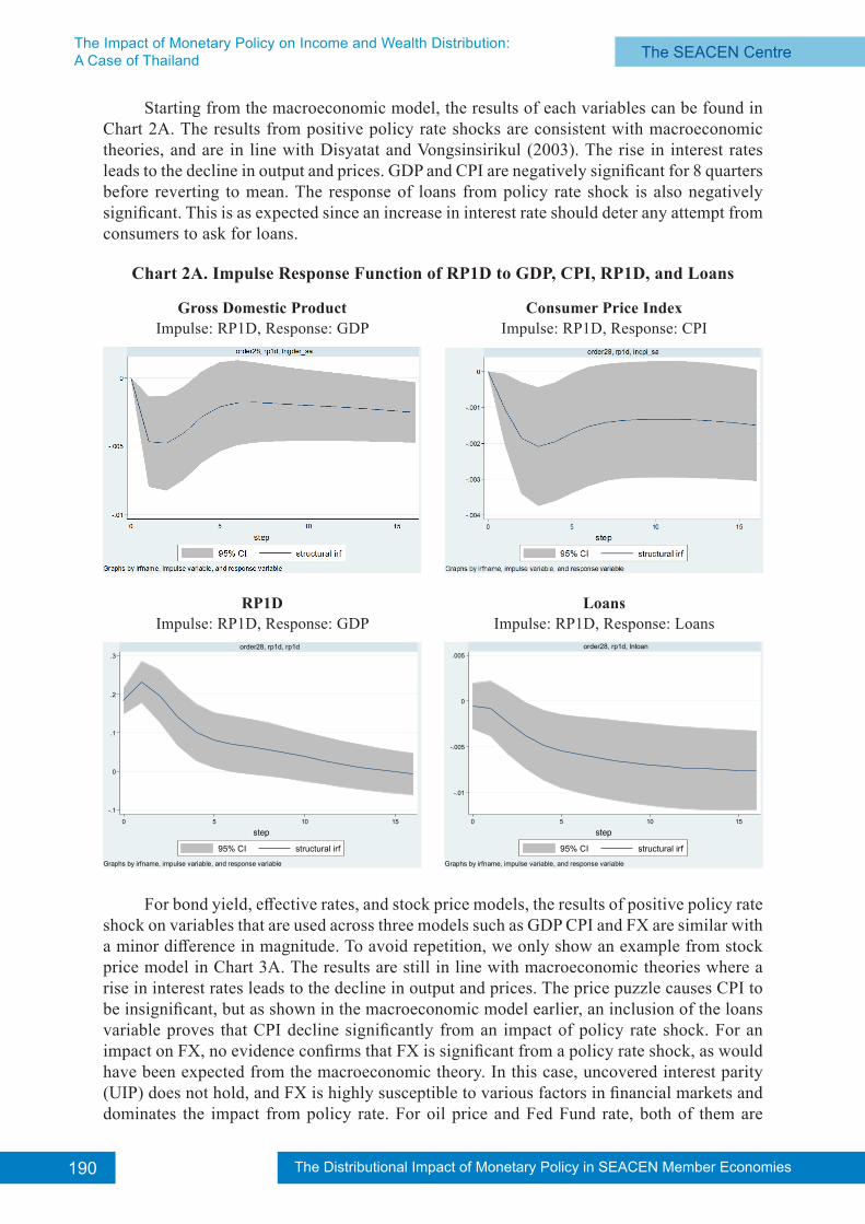
Starting from the macroeconomic model, the results of each variables can be found in Chart 2A. The results from positive policy rate shocks are consistent with macroeconomic theories, and are in line with Disyatat and Vongsinsirikul (2003). The rise in interest rates leads to the decline in output and prices. GDP and CPI are negatively significant for 8 quarters before reverting to mean. The response of loans from policy rate shock is also negatively significant. This is as expected since an increase in interest rate should deter any attempt from consumers to ask for loans.

Chart 2A. Impulse Response Function of RP1D to GDP, CPI, RP1D, and Loans

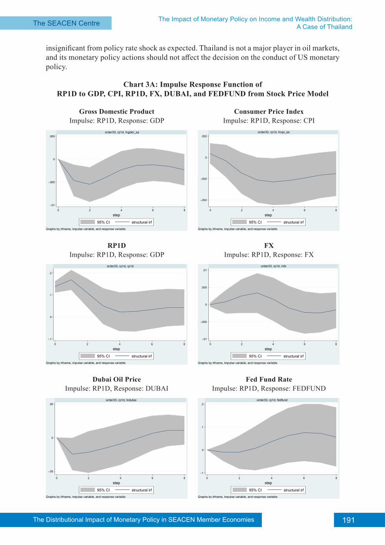
For bond yield, effective rates, and stock price models, the results of positive policy rate shock on variables that are used across three models such as GDP CPI and FX are similar with a minor difference in magnitude. To avoid repetition, we only show an example from stock price model in Chart 3A. The results are still in line with macroeconomic theories where a rise in interest rates leads to the decline in output and prices. The price puzzle causes CPI to be insignificant, but as shown in the macroeconomic model earlier, an inclusion of the loans variable proves that CPI decline significantly from an impact of policy rate shock. For an impact on FX, no evidence confirms that FX is significant from a policy rate shock, as would have been expected from the macroeconomic theory. In this case, uncovered interest parity (UIP) does not hold, and FX is highly susceptible to various factors in financial markets and dominates the impact from policy rate. For oil price and Fed Fund rate, both of them are

-.1

0

.1

.2

.3

0 5 10 15

order28, rp1d, rp1d


step




LoansImpulse: RP1D, Response: Loans

RP1DImpulse: RP1D, Response: GDP

-.01

-.005

0

.005

0 5 10 15

order28, rp1d, lnloan


step



A Case of Thailand

insignificant from policy rate shock as expected. Thailand is not a major player in oil markets, and its monetary policy actions should not affect the decision on the conduct of US monetary policy.

Chart 3A: Impulse Response Function of RP1D to GDP, CPI, RP1D, FX, DUBAI, and FEDFUND from Stock Price Model



FXImpulse: RP1D, Response: FX

RP1DImpulse: RP1D, Response: GDP

Fed Fund RateImpulse: RP1D, Response: FEDFUND

Dubai Oil PriceImpulse: RP1D, Response: DUBAI

-.1

0

.1

.2

0 2 4 6 8

order33, rp1d, rp1d


step


-.01

-.005

0

.005

.01

0 2 4 6 8

order33, rp1d, lnfx


step


-.05

0

.05

0 2 4 6 8

order33, rp1d, lndubai


step


-.1

0

.1

.2

0 2 4 6 8

order33, rp1d, fedfund


step


-.01

-.005

0

.005

0 2 4 6 8

order33, rp1d, lngder_sa


step


-.004

-.002

0

.002

0 2 4 6 8

order33, rp1d, lncpi_sa


step



A Case of Thailand

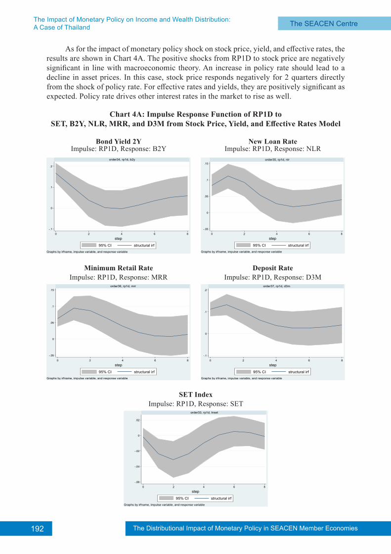
As for the impact of monetary policy shock on stock price, yield, and effective rates, the results are shown in Chart 4A. The positive shocks from RP1D to stock price are negatively significant in line with macroeconomic theory. An increase in policy rate should lead to a decline in asset prices. In this case, stock price responds negatively for 2 quarters directly from the shock of policy rate. For effective rates and yields, they are positively significant as expected. Policy rate drives other interest rates in the market to rise as well.

Chart 4A: Impulse Response Function of RP1D to SET, B2Y, NLR, MRR, and D3M from Stock Price, Yield, and Effective Rates Model

New Loan RateImpulse: RP1D, Response: NLR

Bond Yield 2YImpulse: RP1D, Response: B2Y

Deposit RateImpulse: RP1D, Response: D3M

Minimum Retail RateImpulse: RP1D, Response: MRR

SET IndexImpulse: RP1D, Response: SET

-.1

0

.1

.2

0 2 4 6 8

order34, rp1d, b2y


step


-.05

0

.05

.1

.15

0 2 4 6 8

order35, rp1d, nlr


step


-.05

0

.05

.1

.15

0 2 4 6 8

order36, rp1d, mrr


step


-.1

0

.1

.2

0 2 4 6 8

order37, rp1d, d3m


step


-.06

-.04

-.02

0

.02

0 2 4 6 8

order33, rp1d, lnset


step



A Case of Thailand

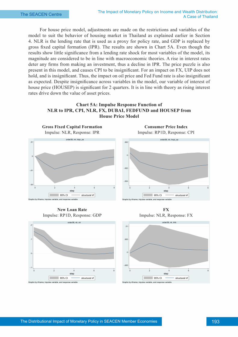
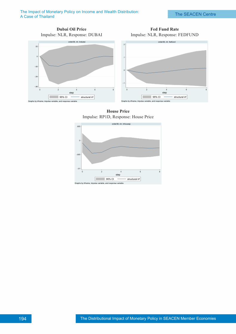
For house price model, adjustments are made on the restrictions and variables of the model to suit the behavior of housing market in Thailand as explained earlier in Section 4. NLR is the lending rate that is used as a proxy for policy rate, and GDP is replaced by gross fixed capital formation (IPR). The results are shown in Chart 5A. Even though the results show little significance from a lending rate shock for most variables of the model, its magnitude are considered to be in line with macroeconomic theories. A rise in interest rates deter any firms from making an investment, thus a decline in IPR. The price puzzle is also present in this model, and causes CPI to be insignificant. For an impact on FX, UIP does not hold, and is insignificant. Thus, the impact on oil price and Fed Fund rate is also insignificant as expected. Despite insignificance across variables in the model, our variable of interest of house price (HOUSEP) is significant for 2 quarters. It is in line with theory as rising interest rates drive down the value of asset prices.

Chart 5A: Impulse Response Function ofNLR to IPR, CPI, NLR, FX, DUBAI, FEDFUND and HOUSEP from

House Price Model


Gross Fixed Capital FormationImpulse: NLR, Response: IPR

FXImpulse: NLR, Response: FX

New Loan RateImpulse: RP1D, Response: GDP

-.02

-.01

0

.01

0 2 4 6 8

order38, nlr, lnipr_sa


step


-.004

-.002

0

.002

0 2 4 6 8

order38, nlr, lncpi_sa


step


-.1

0

.1

.2

0 2 4 6 8

order38, nlr, nlr


step


-.005

0

.005

.01

0 2 4 6 8

order38, nlr, lnfx


step



A Case of Thailand

Fed Fund RateImpulse: NLR, Response: FEDFUND

Dubai Oil PriceImpulse: NLR, Response: DUBAI

House PriceImpulse: RP1D, Response: House Price

-.06

-.04

-.02

0

.02

0 2 4 6 8

order38, nlr, lndubai


step


-.1

0

.1

.2

0 2 4 6 8

order38, nlr, fedfund


step


-.01

-.005

0

.005

0 2 4 6 8

order38, nlr, lnhousep


step


Documents

THE IMPACT OF MONETARY POLICY ON INCOME AND WEALTH