The Impact of Midbrain Cauterize Size on Auditory and Visual

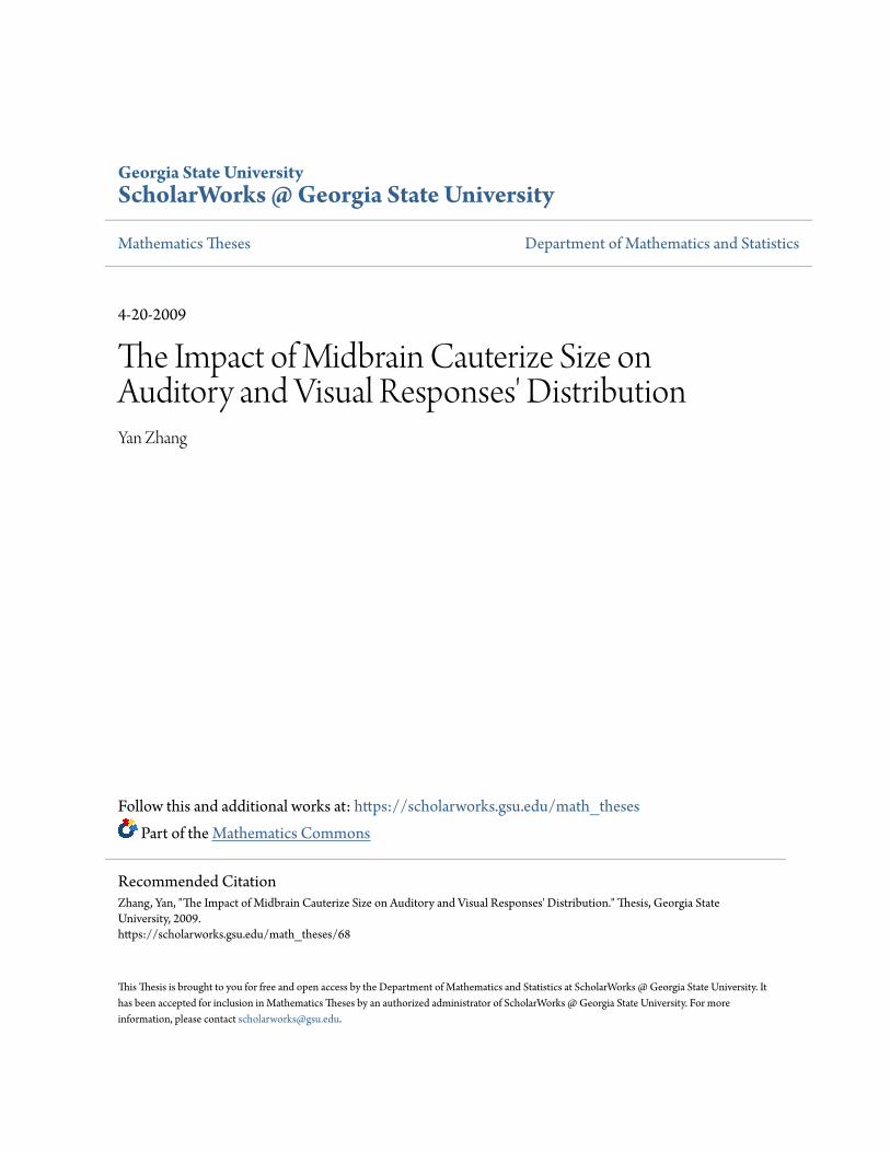
Georgia State UniversityScholarWorks @ Georgia State University

Mathematics Theses Department of Mathematics and Statistics

4-20-2009

The Impact of Midbrain Cauterize Size onAuditory and Visual Responses' DistributionYan Zhang

Follow this and additional works at: https://scholarworks.gsu.edu/math_theses

Part of the Mathematics Commons

This Thesis is brought to you for free and open access by the Department of Mathematics and Statistics at ScholarWorks @ Georgia State University. Ithas been accepted for inclusion in Mathematics Theses by an authorized administrator of ScholarWorks @ Georgia State University. For moreinformation, please contact [email protected].

Recommended CitationZhang, Yan, "The Impact of Midbrain Cauterize Size on Auditory and Visual Responses' Distribution." Thesis, Georgia StateUniversity, 2009.https://scholarworks.gsu.edu/math_theses/68

https://scholarworks.gsu.edu?utm_source=scholarworks.gsu.edu%2Fmath_theses%2F68&utm_medium=PDF&utm_campaign=PDFCoverPages

https://scholarworks.gsu.edu/math_theses?utm_source=scholarworks.gsu.edu%2Fmath_theses%2F68&utm_medium=PDF&utm_campaign=PDFCoverPages

https://scholarworks.gsu.edu/math?utm_source=scholarworks.gsu.edu%2Fmath_theses%2F68&utm_medium=PDF&utm_campaign=PDFCoverPages

https://scholarworks.gsu.edu/math_theses?utm_source=scholarworks.gsu.edu%2Fmath_theses%2F68&utm_medium=PDF&utm_campaign=PDFCoverPages

http://network.bepress.com/hgg/discipline/174?utm_source=scholarworks.gsu.edu%2Fmath_theses%2F68&utm_medium=PDF&utm_campaign=PDFCoverPages

mailto:[email protected]

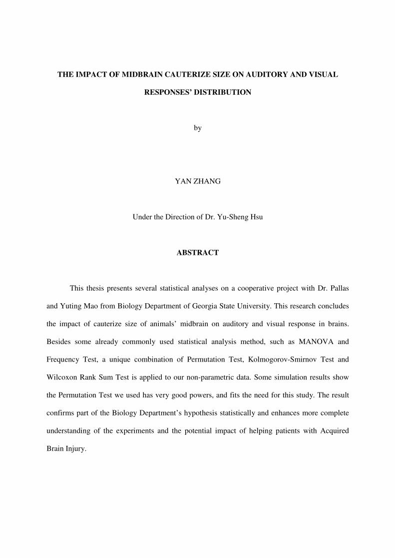
THE IMPACT OF MIDBRAIN CAUTERIZE SIZE ON AUDITORY AND VISUAL

RESPONSES’ DISTRIBUTION

by

YAN ZHANG

Under the Direction of Dr. Yu-Sheng Hsu

ABSTRACT

This thesis presents several statistical analyses on a cooperative project with Dr. Pallas

and Yuting Mao from Biology Department of Georgia State University. This research concludes

the impact of cauterize size of animals’ midbrain on auditory and visual response in brains.

Besides some already commonly used statistical analysis method, such as MANOVA and

Frequency Test, a unique combination of Permutation Test, Kolmogorov-Smirnov Test and

Wilcoxon Rank Sum Test is applied to our non-parametric data. Some simulation results show

the Permutation Test we used has very good powers, and fits the need for this study. The result

confirms part of the Biology Department’s hypothesis statistically and enhances more complete

understanding of the experiments and the potential impact of helping patients with Acquired

Brain Injury.

INDEX WORDS: MANOVA, Frequency Test, Kolmogorov-Smirnov Test, Wilcoxon Rank Sum

Test, Pearson Chi-square Test, Fisher’s Exact Test, Permutation Test



by

YAN ZHANG

A Thesis Submitted in Partial Fulfillment of the Requirements for the Degree of

Master of Science

in the College of Arts and Sciences

Georgia State University

2009

Copyright by

Yan Zhang

2009



by

YAN ZHANG

Major Professor: Dr. Yu-Sheng Hsu

Committee: Dr. Sarah. L. Pallas

Dr. Xu Zhang

Electronic Version Approved:

Office of Graduate Studies

College of Art and Sciences

Georgia State University

May 2009

iv

ACKNOWLEDGEMENTS

First and foremost, my deepest gratitude goes to my advisor, Dr. Yu-Sheng Hsu,

professor and graduate director of Statistics. This thesis would not have been possible without

his encouragement and guidance.

I would also like to thank my committee member, Dr. Sarah Pallas for the time you spent

to go through my thesis and also your insightful comments. I would like to give my appreciation

to another committee member, Dr. Xu Zhang for helping me several times with my SAS

programming and thesis advice. I sincerely appreciate all your input to help me complete my

thesis.

I would also like to thank Yuting Mao, a graduate student in Biology Department, for

your hard work in producing so many data sets, providing me the background information of this

study and the communication between us.

Lastly, I would like to thank my family, friends, who have shown tremendous support

during this education process.

v

TABLE OF CONTENTS

ACKNOWLEDGEMENTS iv

LIST OF TABLES vii

LIST OF FIGURES viii

LIST OF ABBREVIATIONS ix

CHAPTER ONE: INTRODUCTION 1

1.1 Background 1

1.2 Source of Data 2

CHAPTER TWO: METHOD OF ANALYSIS 7

2.1 Frequency Test 7

2.2 Multivariate Analysis of Variance (MANOVA) Test 8

2.3 Permutation Test 8

2.3.1 Kolmogorov-Smirnov Test 10

2.3.2 Wilcoxon Rank Sum Test 11

2.3.3 Permutation Test 12

CHAPTER THREE: RESULTS AND DISCUSSIONS 14

3.1 Frequency Test Result 14

3.2 MANOVA Test to Show the Impact of Three Factors on the Location of the 15

Response Points

3.3 Permutation Test to Detect the Distribution Difference of Same Colored Points 21

from Different Lesion Groups

CHAPTER FOUR: CONCLUSION AND FUTURE RESEARCH 24

REFERENCES 26

vi

APPENDICES

Appendix A: SAS Code 27

Appendix B: SAS Output 43

vii

LIST OF TABLES

Table 1 Percentage composition of each color group within each lesion group 15

Table 2 MANOVA table of all data: Impact of three factors on x 16

Table 3 MANOVA table of all data: Impact of three factors on y 16

Table 4 P-value table of MANOVA on all data: Testing overall factor effect 16

Table 5 MANOVA table of Control group data: Impact of two factors on x and y 18

Table 6 P-value of MANOVA on Control group: Testing overall factor effect 18

Table 7 MANOVA table of Small lesion group: Impact of two factors on x and y 19

Table 8 P-values of MANOVA on Small lesion group: Testing overall factor effect 19

Table 9 MANOVA table of Large lesion group: Impact of two factors on x and y 20

Table 10 P-values of MANOVA on Large lesion group: Testing overall factor effect 20

Table 11 Permutation Test simulation table 22

Table 12 Permutation Test result (P-value table) of same color dots between lesion 23

groups

viii

LIST OF FIGURES

Figure 1 Cartesion plot on AI 3

Figure 2 Control group 4

Figure 3 Small lesion group 5

Figure 4 Large lesion group 6

Figure 5 Illustration of KS-test’s D statistic 11

Figure 6 Proportion compositions 14

ix

LIST OF ABBREVIATIONS

ABI Acquired Brain Injury

AI Primary Auditory Cortex

MANOVA Multivariate Analysis of Variance

KS-Test Kolmogorov-Smirnov Test

MRI Magnetic Resonance Imaging

1

CHAPTER ONE: INTRODUCTION

1.1 Background

Acquired Brain Injury (ABI) is a serious clinical problem. It can be caused by traumatic

brain injury (physical trauma) and non-traumatic brain injury (stroke, brain tumor, etc.). ABI can

affect cognitive, physical, emotional, social and any other functions in the brain. The outcomes

of ABI range from complete recovery to death or permanent disability, largely depending on the

severity of the injury and timely receipt of appropriate treatment. The demand to save lives of

soldiers from traumatic brain damage is increasing because of the increased incidence of closed

head, blast-induced injury in war zones. The knowledge from research on ABI will not only help

to understand the mechanisms that underlie ABI, but may also be applied to improve medical

treatment of patients with ABI.

Research on ABI has primarily concentrated on recovery from injury and compensatory

plasticity. Compared to other models such as congenitally deaf animals, the cross-modal

plasticity model initialized by Dr. Sarah Pallas and her assistant Yuting Mao is especially

suitable for studying ABI, taking the advantage of neonatal injury in brain areas. In their model

system, midbrain lesions cause visual afferents to project to auditory thalamus. This process is an

example of the process of recovery from brain injury. The primary auditory cortex is then

reorganized across modalities, providing an example of compensatory plasticity. This model

offers an opportunity to several future research topics on ABI. We only helped analyzing the

auditory and visual responses’ distribution on the primary auditory cortex after the ABI using

appropriate statistical methods.

2

The cross-modal plasticity model initialized by Dr. Sarah Pallas and Yuting Mao uses

ferrets as the experimental subjects. They cauterized midbrain of ferrets at postnatal day one.

Each animal was scanned by Magnetic Resonance Imaging (MRI) to confirm the midbrain

lesions. In vivo extracellular recording was performed in adulthood. Auditory, visual and

bimodal stimuli were applied during recording. Electrical stimulation of the optic chiasm was

used to activate optic nerves directly in the event that there was no response to light. Normal

animals without any surgery were used as a control for the lesion group.

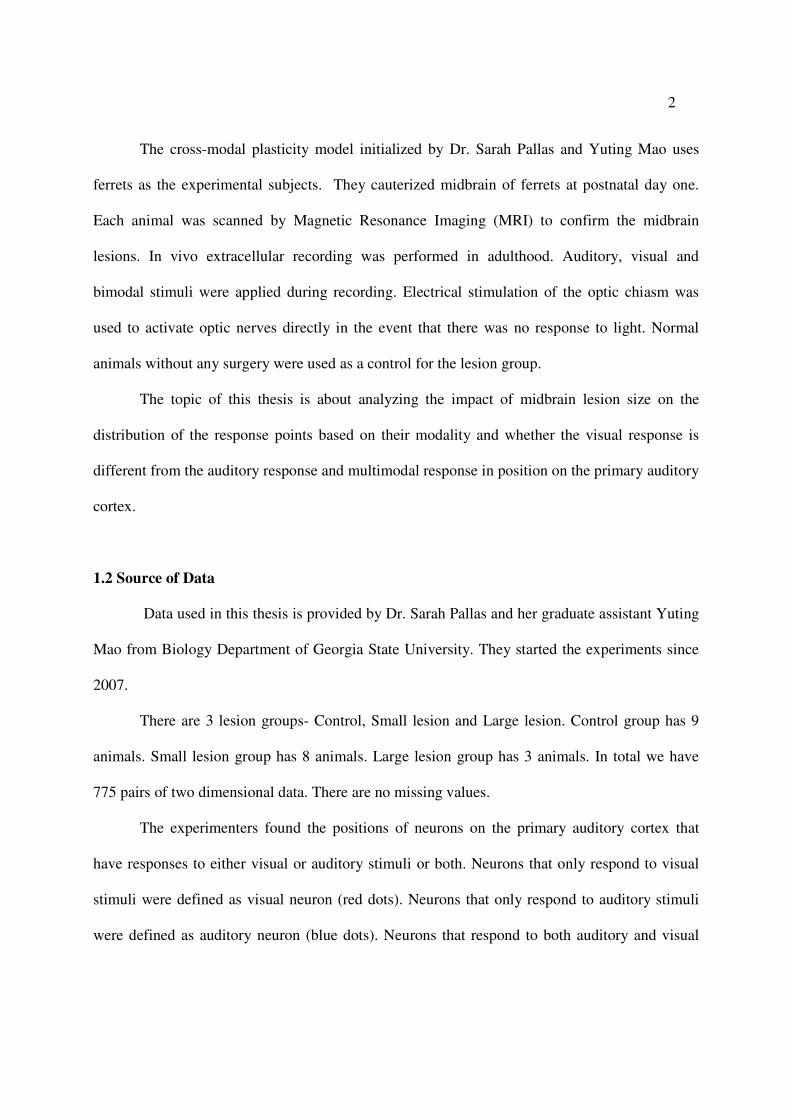
The topic of this thesis is about analyzing the impact of midbrain lesion size on the

distribution of the response points based on their modality and whether the visual response is

different from the auditory response and multimodal response in position on the primary auditory

cortex.

1.2 Source of Data

Data used in this thesis is provided by Dr. Sarah Pallas and her graduate assistant Yuting

Mao from Biology Department of Georgia State University. They started the experiments since

2007.

There are 3 lesion groups- Control, Small lesion and Large lesion. Control group has 9

animals. Small lesion group has 8 animals. Large lesion group has 3 animals. In total we have

775 pairs of two dimensional data. There are no missing values.

The experimenters found the positions of neurons on the primary auditory cortex that

have responses to either visual or auditory stimuli or both. Neurons that only respond to visual

stimuli were defined as visual neuron (red dots). Neurons that only respond to auditory stimuli

were defined as auditory neuron (blue dots). Neurons that respond to both auditory and visual

3

stimuli were defined as multimodal neurons (dots that have both blue and red colors). Neurons

that only respond to one modality and can be significantly modulated by another modality were

defined as multimodal neurons (dots that have both blue and red colors). The first version of the

data and the illustrations of the animals’ brain indicated multimodal neurons with green color.

Only at the final step of our analysis, Yuting Mao updated their data using dots of both blue and

red color for multimodal neurons. We could see that from updated Figure2, Figure 3 and Figure

4. But our code and some preparation work and graphs already used green color for multimodal

neurons. We will still use green color to indicate multimodal neurons through this paper for our

convenience.

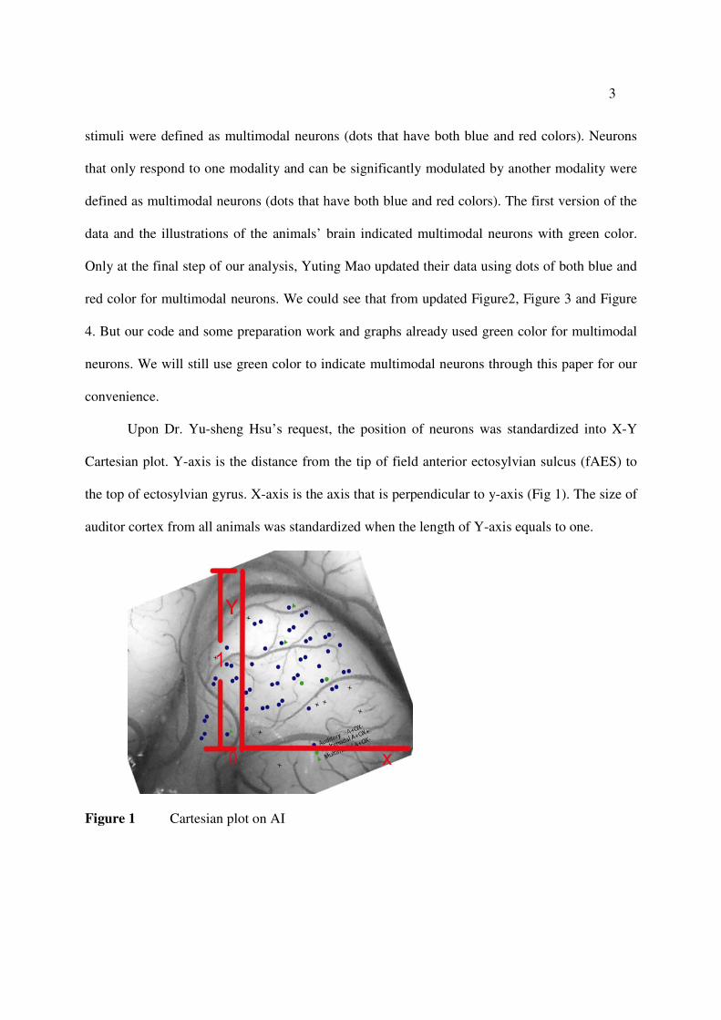
Upon Dr. Yu-sheng Hsu’s request, the position of neurons was standardized into X-Y

Cartesian plot. Y-axis is the distance from the tip of field anterior ectosylvian sulcus (fAES) to

the top of ectosylvian gyrus. X-axis is the axis that is perpendicular to y-axis (Fig 1). The size of

auditor cortex from all animals was standardized when the length of Y-axis equals to one.

Figure 1 Cartesian plot on AI

4

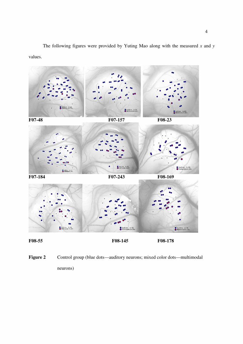
The following figures were provided by Yuting Mao along with the measured x and y

values.

F07-48 F07-157 F08-23

F07-184 F07-243 F08-169

F08-55 F08-145 F08-178

Figure 2 Control group (blue dots—auditory neurons; mixed color dots—multimodal

neurons)

5

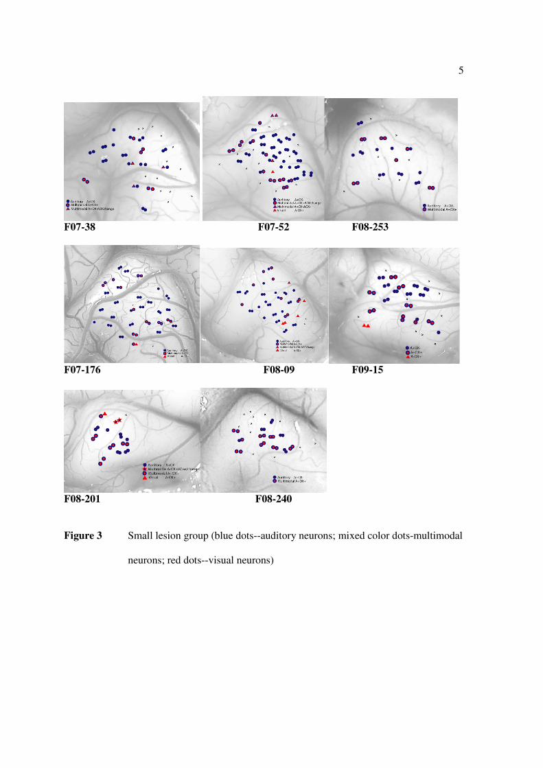
F07-38 F07-52 F08-253

F07-176 F08-09 F09-15

F08-201 F08-240

Figure 3 Small lesion group (blue dots--auditory neurons; mixed color dots-multimodal

neurons; red dots--visual neurons)

6

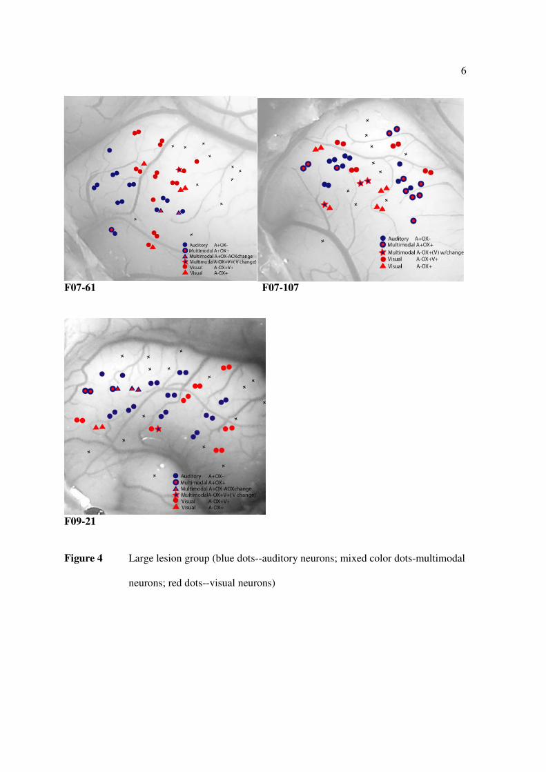
F07-61 F07-107

F09-21

Figure 4 Large lesion group (blue dots--auditory neurons; mixed color dots-multimodal

neurons; red dots--visual neurons)

7

CHAPTER TWO: METHOD OF ANALYSIS

In this chapter, we discuss and review the techniques elected to analyze the provided data

and then draw the conclusion. We first did a Frequency Test to get a general idea of the data. On

our second step, to test the impact of three selected potential factors on the location of those

response dots (in terms of x and y), we applied MANOVA test on all the data as a whole and

then within each lesion group. Last, under Dr Hsu’s guidance, we used a unique combination of

Kolmogorov Smirnov test, Wilcoxon Rank Sum Test and Permutation Test on the two

dimensional data to detect any distribution difference on same color points from different lesion

groups.

2.1 Frequency Test

Frequency Test is very commonly used in statistics analysis. In our analysis, we are

interested in the frequency test on two classification cross table since we want to know if there is

any association between factor color and factor lesion size. In this case the null hypothesis is that

the two factors are independent.

From the contingency table of factor color and factor lesion size, we could already see the

change of the percentage of each color within each lesion size group. Furthermore, we requested

both Pearson Chi-square Test and Fisher’s Exact Test through SAS code to obtain the P-value.

Fisher’s Exact Probability is requested because Fisher’s Exact Probability is not plagued by

inaccuracies due to small number of observations. We noticed that some animals have only one

or two observations for certain colors.

8

2.2 Multivariate Analysis of Variance (MANOVA) Test

In our analysis, we are interested in knowing if the location of response points is affected

by the following three factors: Which animal do these points belong to? What color are these

points? And what kind of lesion was this animal given? Since the location is indicated by x and

y, MANOVA Test answers these questions by testing the hypothesis on the means of (x, y) for

each group of points applying these three independent factors----lesion size, color and individual

animal. The factor, individual animal, is nested within factor lesion size.

2.3 Permutation Test

The last topic of interest is to detect that whether points of the same color between

different lesion groups have same distributions. This part of analysis was initialed by Dr. Hsu

using a unique combination of three non-parametric methods and is the emphasis of this thesis. It

was programmed by us because there are no available functions ready to use in SAS. I’d like to

introduce our methodology in details about this part.

The most common methods for inference about means based on a single sample, matched

pairs, or two independent samples (our case) are the t procedures. We always rely on the

assumption of normal distribution for data but no data are exactly normal. The t procedures are

robust, quite insensitive to deviations from normality in the data. But we usually need quite large

samples. The datasets we were given are typical biology experiment outcomes. We have small

number of objects---9 Control group animals, 8 Small lesion animals and 3 Large lesion animals.

Besides the limited number of observations, these three groups of observations are not balanced.

Obviously, it is not appropriate to use traditional inference on our limited datasets. We used

Permutation Test because it keeps the computing power but relax some of the conditions needed

9

for traditional inference. We don’t know what kind of distribution those response points have

and each animal’s response to the lesion surgery is quite individual. Permutation Test sets us free

from the need for normal data or large samples and it also set us free from formulas or

distributions. It also works well for unbalance data like ours. Because of its effectiveness and

range of great use, Permutation Test along with other randomization test is becoming the

preferred way to do statistical inference. It is already true in some areas such as clinical trial and

bio-medical research. It can, with sufficient computing power, gives results that are more

accurate than those from traditional methods. So before we applied the permutation test on the

real data, we first did the simulation to check the power of the test. The results are actually better

than we expected. Please refer to the simulation table in the discussion chapter.

We first decided that the test statistics to detect the distribution difference is a measure of

“distance” between two multivariate distributions. We selected Kolmogorov-Smirnov Distance.

The available K-S Test in SAS is only for one dimension data so we tailored our own code for

our two dimensional data. Then we did a transfer of our test statistics from the solid number of

“distance” out of any two animals to its corresponding rank then to the Rank Sum of all the

animals in one lesion size population using Wilcoxon Rank Sum Test. After that we used

Permutation Test to list all the possible rank sums from all possible ways of relocating animals to

two groups and obtained the significance test result. We cannot use the approximate distribution

of the Wilcoxon Rank Sum statistic because the “independent” condition is not satisfied in this

Permutation Test.

10

2.3.1. Kolmogorov-Smirnov Test

First, we selected a measure of distance between two multivariate distributions. We used

the two-sample Kolmogorov-Smirnov Test (KS-test). It tries to determine if two distributions

differ significantly, i.e., to test whether two samples come from the same distributions. The KS-

test has the advantage of making no assumption about the distribution of data. Technically

speaking it is non-parametric and distribution free.

We have animal #1 with n1 response points and animal #2 with n2 response points. When

you mix these two animals’ response points, for each dot of (x, y) from the mixed pool, you will

find 1nF and 2nF , where ∑=

≤=

n

i

yxYXn iI

nyxF

1

),(),(

1),( . Use the following formula, you will find a D

given any two animals’ response points.

),(),(sup 21),(

2,1 yxFyxFD nnyx

nn −=

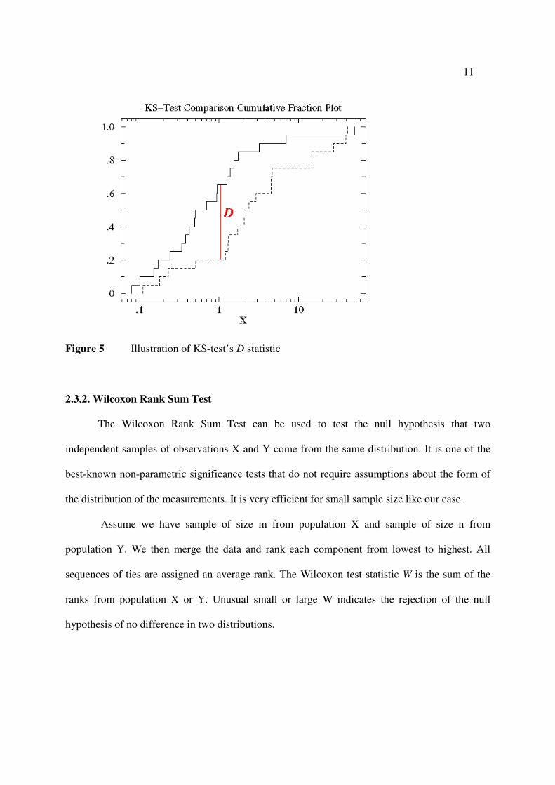
If the two animals’ same colored points are distributed at approximately same location,

their cumulative fraction plots should be close to each other, producing small value of D statistic.

If the two animals’ same colored points are distributed far away from each other, their data will

give us large value of D statistic.

Suppose we have M animals from lesion group 1 and N animals from lesion group 2.

Since we can work out a D statistic for any two animals, we will have

2

M Ds if both animals

are from lesion group 1 and

2

N Ds if both animals are from lesion group 2. There are M*N Ds

if one animal from each lesion group. We will see this equation:

+

=+

+

2*

22

NMNM

NM

11

Figure 5 Illustration of KS-test’s D statistic

2.3.2. Wilcoxon Rank Sum Test

The Wilcoxon Rank Sum Test can be used to test the null hypothesis that two

independent samples of observations X and Y come from the same distribution. It is one of the

best-known non-parametric significance tests that do not require assumptions about the form of

the distribution of the measurements. It is very efficient for small sample size like our case.

Assume we have sample of size m from population X and sample of size n from

population Y. We then merge the data and rank each component from lowest to highest. All

sequences of ties are assigned an average rank. The Wilcoxon test statistic W is the sum of the

ranks from population X or Y. Unusual small or large W indicates the rejection of the null

hypothesis of no difference in two distributions.

12

Now Wilcoxon Rank Sum Test is applied on all the

+

2

NM D statistics worked out

from step I. We consider

+

22

NM Ds are from population X, which means both animals are

from the same lesion group and the Ds are relatively small, so the assigned ranks on them are

also small. While NM * Ds are from population Y, which means two animals are from different

lesion group and the Ds are relatively large, therefore the assigned ranks on them are also large.

If we use the rank sum of population X, small statistic W would lead us to reject null

hypothesis of no distribution difference of same colored points from different lesion groups. For

the convenience of our program writing, we used the rank sum of population Y as the Wilcoxon

Test statistics. Therefore, large number result in our program code leads to the rejection of null

hypothesis.

2.3.3. Permutation Test

Now with the test statistic W from the above Wilcoxon Rank Sum step, we will do the

statistical significance test to see if we can reject null hypothesis or not. Since we don’t know

either the distribution of the points or the distribution of Wilcoxon Rank Sum statistic from last

step due to the dependency of X and Y, we chose to do the Permutation Test.

Permutation test (also called a randomization test) has the advantage of being a non-

parametric statistics test. It is a type of statistical significance test in which a reference

distribution is obtained by calculating all possible values of the test statistics under

rearrangements of the labels on the observed data points. If the labels are exchangeable under the

null hypothesis, then the resulting tests yield exact significance levels.

13

An important assumption behind a Permutation Test is that the observations are

exchangeable under the null hypothesis. Our project has this assumption to start Permutation

Test with. Under the null hypothesis, we assume the same colored points from different lesion

groups come from the same distribution. Suppose we have two groups A and B. Let nA and nB be

the sample size corresponding to each group. The permutation test is designed to determine

whether the Wilcoxon Rank Sum of population Y (two animals are from different lesion groups)

is large enough to reject the null hypothesis H0 that the two groups’ same colored points have

same distribution. The test proceeds as follows. First, the actual Rank Sum W is calculated: this

is the observed value of the test statistic. Then the observations of groups A and B are pooled.

Next, the Rank Sum W is calculated and recorded for every possible way of dividing these

pooled values into two groups of size nA and nB (i.e., for every permutation of the group labels A

and B). The set of these calculated rank sum Ws is the exact distribution of all possible test

statistic Ws under the null hypothesis that group label does not matter. In our test, we sorted the

entire recorded test statistic Ws, and then see if the observed value of W from first step is

contained within the lower 95% of them. If the observed W belongs to the upper 5%, we reject

the null hypothesis of identical distribution for same colored points from different lesion groups

at the 5% significant level.

Before we did this test, we did simulation to see the power of this Permutation Test

combined with Kolmogorov-Smirnov Test and Wilcoxon Rank Sum Test. We will discuss the

result in our next chapter.

14

CHAPTER THREE: RESULTS AND DISCUSSIONS

Now, let’s look at the analysis results when we apply the techniques mentioned in

Chapter two to the provided data.

3.1 Frequency Test Result

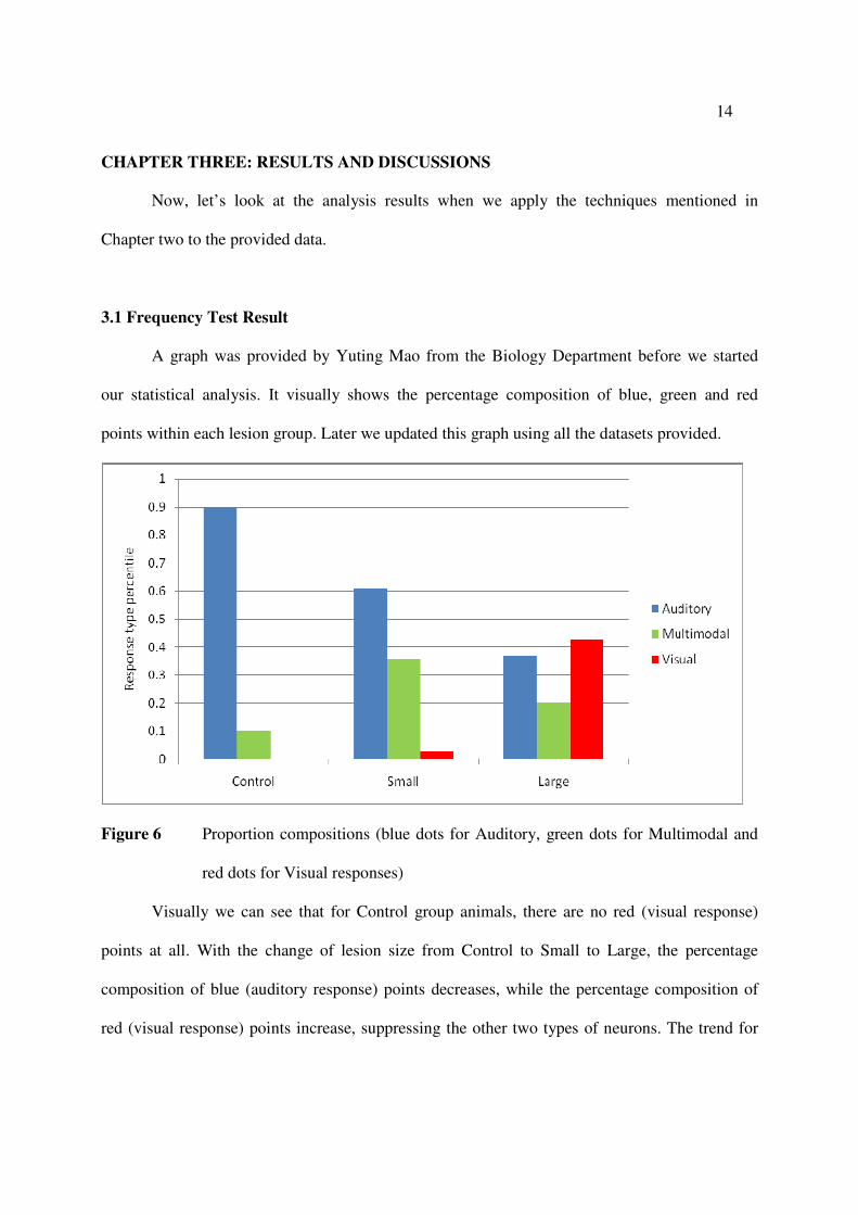
A graph was provided by Yuting Mao from the Biology Department before we started

our statistical analysis. It visually shows the percentage composition of blue, green and red

points within each lesion group. Later we updated this graph using all the datasets provided.

Figure 6 Proportion compositions (blue dots for Auditory, green dots for Multimodal and

red dots for Visual responses)

Visually we can see that for Control group animals, there are no red (visual response)

points at all. With the change of lesion size from Control to Small to Large, the percentage

composition of blue (auditory response) points decreases, while the percentage composition of

red (visual response) points increase, suppressing the other two types of neurons. The trend for

15

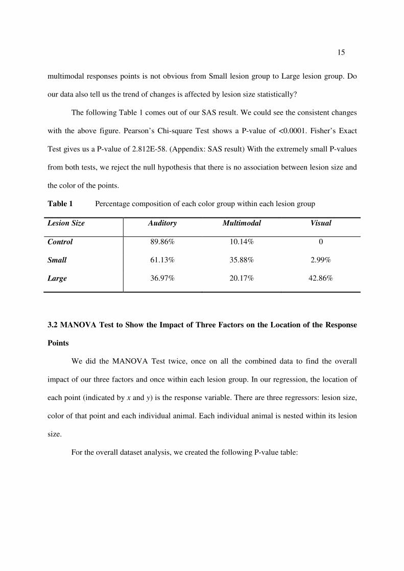
multimodal responses points is not obvious from Small lesion group to Large lesion group. Do

our data also tell us the trend of changes is affected by lesion size statistically?

The following Table 1 comes out of our SAS result. We could see the consistent changes

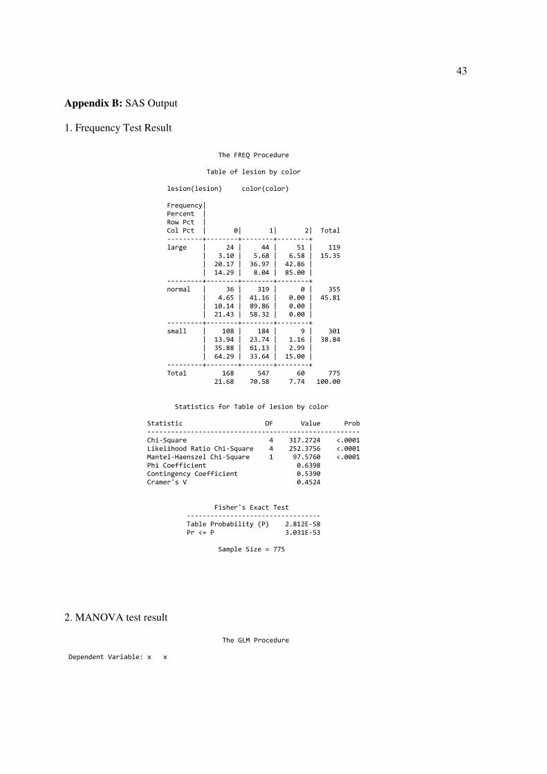
with the above figure. Pearson’s Chi-square Test shows a P-value of <0.0001. Fisher’s Exact

Test gives us a P-value of 2.812E-58. (Appendix: SAS result) With the extremely small P-values

from both tests, we reject the null hypothesis that there is no association between lesion size and

the color of the points.

Table 1 Percentage composition of each color group within each lesion group

Lesion Size Auditory Multimodal Visual

Control 89.86% 10.14% 0

Small 61.13% 35.88% 2.99%

Large 36.97% 20.17% 42.86%

3.2 MANOVA Test to Show the Impact of Three Factors on the Location of the Response

Points

We did the MANOVA Test twice, once on all the combined data to find the overall

impact of our three factors and once within each lesion group. In our regression, the location of

each point (indicated by x and y) is the response variable. There are three regressors: lesion size,

color of that point and each individual animal. Each individual animal is nested within its lesion

size.

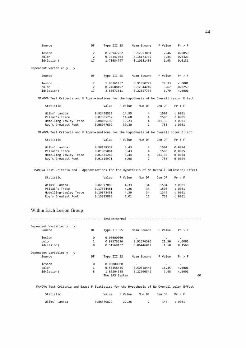
For the overall dataset analysis, we created the following P-value table:

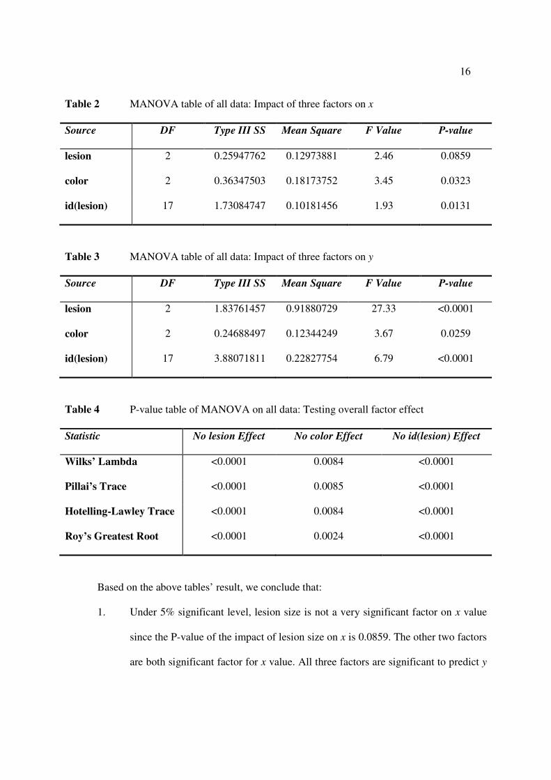
16

Table 2 MANOVA table of all data: Impact of three factors on x

Source DF Type III SS Mean Square F Value P-value

lesion 2 0.25947762 0.12973881 2.46 0.0859

color 2 0.36347503 0.18173752 3.45 0.0323

id(lesion) 17 1.73084747 0.10181456 1.93 0.0131

Table 3 MANOVA table of all data: Impact of three factors on y


lesion 2 1.83761457 0.91880729 27.33 <0.0001

color 2 0.24688497 0.12344249 3.67 0.0259

id(lesion) 17 3.88071811 0.22827754 6.79 <0.0001

Table 4 P-value table of MANOVA on all data: Testing overall factor effect

Statistic No lesion Effect No color Effect No id(lesion) Effect

Wilks’ Lambda <0.0001 0.0084 <0.0001

Pillai’s Trace <0.0001 0.0085 <0.0001

Hotelling-Lawley Trace <0.0001 0.0084 <0.0001

Roy’s Greatest Root <0.0001 0.0024 <0.0001

Based on the above tables’ result, we conclude that:

1. Under 5% significant level, lesion size is not a very significant factor on x value

since the P-value of the impact of lesion size on x is 0.0859. The other two factors

are both significant factor for x value. All three factors are significant to predict y

17

value. Y value is more sensitive to the impact of all three factors than x value.

(result from Table 2 and Table 3)

2. When testing the null hypothesis of No Overall lesion Effect on the location of

points, we found that all the available statistics lead to strong rejection of null

hypothesis.

3. When testing the null hypothesis of No Overall color Effect on the location of

points, we found that all the available statistics lead to strong rejection of null

hypothesis.

4. When testing the null hypothesis of No Overall individual animal Effect on the

location of points, we found that all the available statistics lead to strong rejection

of null hypothesis. (Conclusion 2, 3 and 4 are from Table 4)

The above result shows that all three factors play significant roles in determining the

location of each point.

Then we did the MANOVA Test within each lesion group. Within each lesion group, we

only tested the factor color and individual animal. We had the following P-value tables and

conclusions:

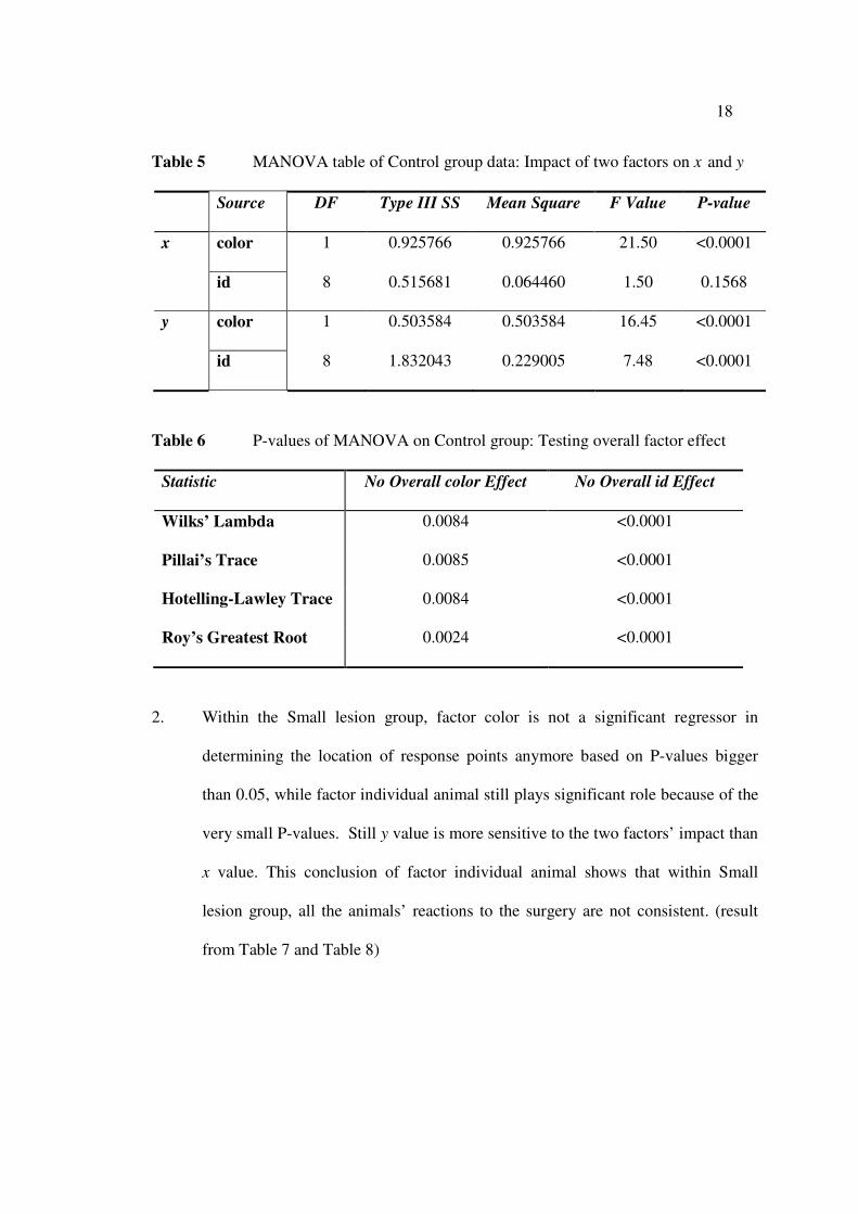
1. Within the Control group, factor color is still a significant factor on the location of a

point. This shows that the auditory response and multimodal response still have their

own distinct locations. Overall individual animal effect is significant in determining

the location but y value is more sensitive to its impact than x value. The P-value of

testing individual animal on x value is 0.1568, not a strong indication of id impact on

x. (result from Table 5 and Table 6)

18

Table 5 MANOVA table of Control group data: Impact of two factors on x and y


x color 1 0.925766 0.925766 21.50 <0.0001

id 8 0.515681 0.064460 1.50 0.1568

y color 1 0.503584 0.503584 16.45 <0.0001

id 8 1.832043 0.229005 7.48 <0.0001

Table 6 P-values of MANOVA on Control group: Testing overall factor effect

Statistic No Overall color Effect No Overall id Effect

Wilks’ Lambda 0.0084 <0.0001

Pillai’s Trace 0.0085 <0.0001

Hotelling-Lawley Trace 0.0084 <0.0001

Roy’s Greatest Root 0.0024 <0.0001

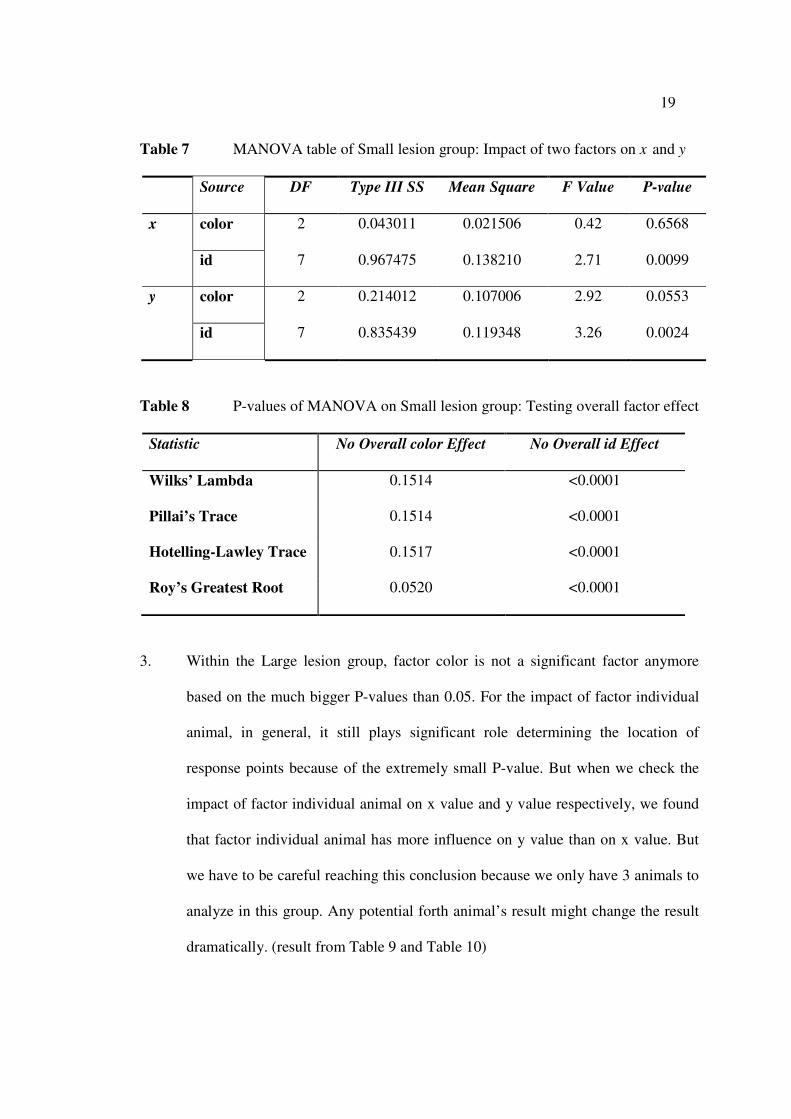
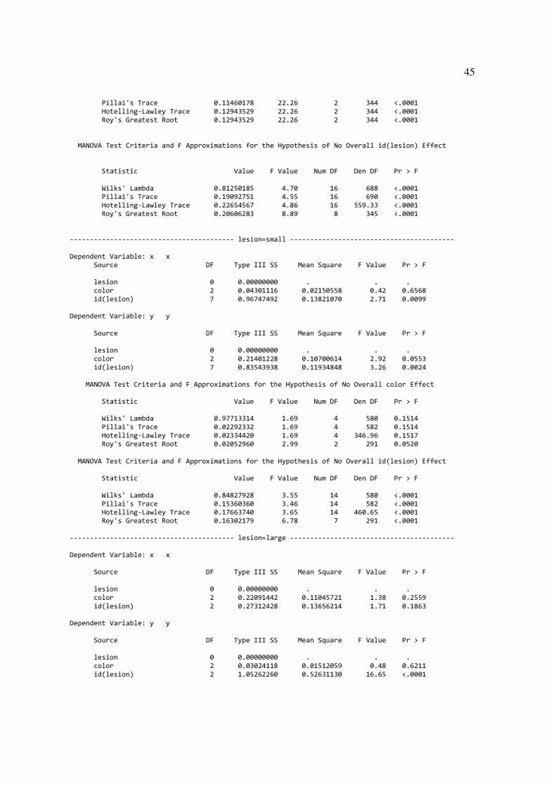
2. Within the Small lesion group, factor color is not a significant regressor in

determining the location of response points anymore based on P-values bigger

than 0.05, while factor individual animal still plays significant role because of the

very small P-values. Still y value is more sensitive to the two factors’ impact than

x value. This conclusion of factor individual animal shows that within Small

lesion group, all the animals’ reactions to the surgery are not consistent. (result

from Table 7 and Table 8)

19

Table 7 MANOVA table of Small lesion group: Impact of two factors on x and y


x color 2 0.043011 0.021506 0.42 0.6568

id 7 0.967475 0.138210 2.71 0.0099

y color 2 0.214012 0.107006 2.92 0.0553

id 7 0.835439 0.119348 3.26 0.0024

Table 8 P-values of MANOVA on Small lesion group: Testing overall factor effect


Wilks’ Lambda 0.1514 <0.0001




3. Within the Large lesion group, factor color is not a significant factor anymore

based on the much bigger P-values than 0.05. For the impact of factor individual

animal, in general, it still plays significant role determining the location of

response points because of the extremely small P-value. But when we check the

impact of factor individual animal on x value and y value respectively, we found

that factor individual animal has more influence on y value than on x value. But

we have to be careful reaching this conclusion because we only have 3 animals to

analyze in this group. Any potential forth animal’s result might change the result

dramatically. (result from Table 9 and Table 10)

20

Table 9 MANOVA table of Large lesion group: Impact of two factors on x and y


x color 2 0.220914 0.110457 1.38 0.2559

id 2 0.273124 0.136562 1.71 0.1863

y color 2 0.030241 0.015121 0.48 0.6211

id 2 1.052622 0.526311 16.65 <0.0001

Table 10 P-values of MANOVA on Large lesion group: Testing overall factor effect


Wilks’ Lambda 0.4537 <0.0001




We can see from the figures provided by the Biology Department that the blue and mixed

color points in Control group’s animals have their own locations---not much mixture of each

other. But for animals in Small lesion and Large lesion group, it seems all colored points are

mingled together, especially the horizontal location (x value). This phenomenon and conclusion

are consistent with the conjecture from Dr. Sarah Pallas and Yuting Mao that after the damage to

the midbrain, during the recovery process, the visual response points start to take over the

primary auditory cortex, where the auditory response were at before the midbrain damage.

21

3.3 Permutation Test to Detect the Distribution Difference of Same Colored Points from

Different Lesion Groups

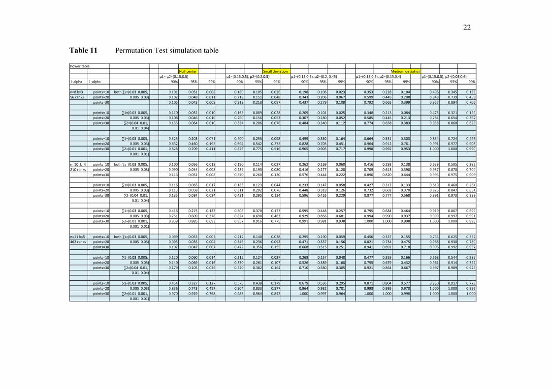
Before we applied the Permutation Test combined with Kolmogorov-Smirnov Test and

Wilcoxon Rank Sum Test to the real data, we carry a simulation study to investigate the power of

the test near the estimated parameter values. Furthermore, we check the powers at the null

hypothesis if they coincide with the significance levels. Hence, the simulation results reflect the

goodness of the method applied to our data. We first create several animals’ data for each

distribution group assuming they have bi-variate normal distribution. After we standardize them

into a Cartesian system, we applied the three steps introduced in Chapter two of this thesis. We

find the power of the test under the null hypothesis situation when the two groups have same

distribution. We also create the situations of increasing numbers of observation to see how good

our method will be when the sample size increases. From Table 11, we can see the powers at null

hypothesis match the significance level we pre-assigned. Just a median deviation of means

or/and variance-covariance matrices, we obtain reasonably powers, which are better than we

originally expected. Therefore, we are comfortable to use this method to test the equality of two-

dimensional distributions. (Table 11)

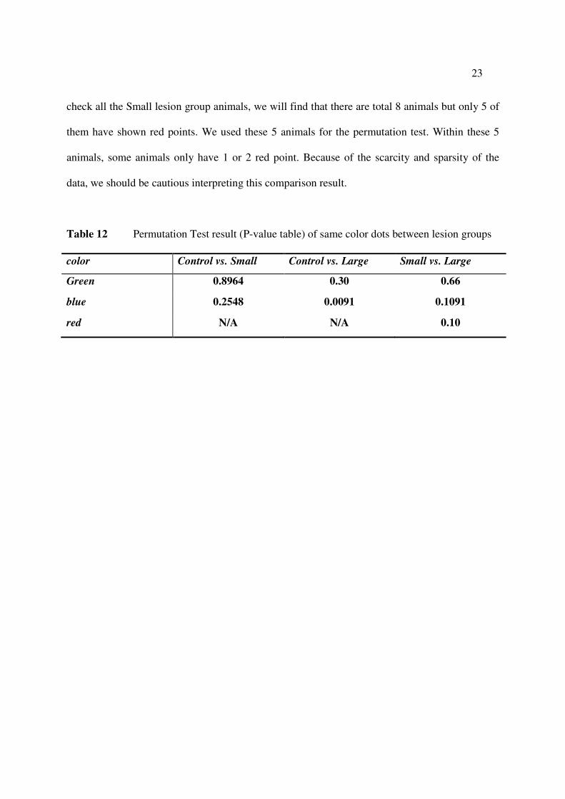
Now we apply the test on real data. The following table is the P-value result of our

Permutation Test on same colored points from different lesion groups. According to the result,

we could only reject the null hypothesis that the blue points between Control group and Large

lesion group have same distribution with strong evidence. For the other scenarios, we could not

detect obvious different distribution patterns. It should be noticed that the comparison of red

points between Small lesion group and Large lesion group gives us a 0.10 P-value. But if we

22

Table 11 Permutation Test simulation table

Power table

Null center Small deviation Medium deviation

μ1= μ2=(0.15,0.5) μ1=(0.15,0.5), μ2=(0.2,0.5) μ1=(0.15,0.5), μ2=(0.2, 0.45) μ1=(0.15,0.5), μ2=(0.15,0.4) μ1=(0.15,0.5), μ2=(0.05,0.6)

1-alpha 1-alpha 90% 95% 99% 90% 95% 99% 90% 95% 99% 90% 95% 99% 90% 95% 99%

n=8 k=3 points=10 both ∑s=(0.03 0.005, 0.101 0.051 0.008 0.180 0.105 0.026 0.198 0.106 0.023 0.353 0.228 0.104 0.496 0.345 0.138

56 ranks points=20 0.005 0.03) 0.102 0.048 0.011 0.218 0.151 0.048 0.343 0.206 0.067 0.599 0.445 0.208 0.848 0.739 0.459

points=30 0.105 0.043 0.008 0.319 0.218 0.087 0.437 0.279 0.108 0.792 0.665 0.399 0.957 0.894 0.706

points=10 ∑1=(0.03 0.005, 0.110 0.052 0.010 0.165 0.089 0.028 0.209 0.101 0.025 0.348 0.213 0.084 0.475 0.321 0.129

points=20 0.005 0.03) 0.108 0.046 0.010 0.260 0.156 0.053 0.307 0.180 0.052 0.585 0.445 0.213 0.784 0.654 0.362

points=30 ∑2=(0.04 0.01, 0.135 0.064 0.010 0.334 0.206 0.076 0.484 0.340 0.112 0.774 0.658 0.383 0.938 0.860 0.625

0.01 0.04)

points=10 ∑1=(0.03 0.005, 0.325 0.203 0.071 0.400 0.255 0.098 0.499 0.350 0.164 0.664 0.531 0.303 0.834 0.724 0.496

points=20 0.005 0.03) 0.632 0.460 0.195 0.694 0.542 0.272 0.828 0.705 0.451 0.964 0.912 0.761 0.991 0.977 0.908

points=30 ∑2=(0.01 0.001, 0.828 0.709 0.411 0.873 0.775 0.516 0.965 0.905 0.717 0.998 0.992 0.953 1.000 1.000 0.990

0.001 0.01)

n=10 k=4 points=10 both ∑s=(0.03 0.005, 0.100 0.056 0.012 0.190 0.114 0.027 0.262 0.169 0.060 0.416 0.293 0.138 0.639 0.505 0.292

210 ranks points=20 0.005 0.03) 0.090 0.044 0.008 0.289 0.193 0.080 0.416 0.277 0.120 0.709 0.613 0.390 0.937 0.870 0.704

points=30 0.116 0.051 0.008 0.370 0.260 0.120 0.576 0.444 0.222 0.890 0.820 0.644 0.993 0.975 0.909

points=10 ∑1=(0.03 0.005, 0.116 0.065 0.017 0.185 0.123 0.044 0.233 0.147 0.058 0.427 0.317 0.133 0.619 0.460 0.264

points=20 0.005 0.03) 0.113 0.058 0.021 0.311 0.202 0.076 0.448 0.318 0.126 0.732 0.602 0.370 0.925 0.847 0.654

points=30 ∑2=(0.04 0.01, 0.135 0.084 0.024 0.431 0.295 0.134 0.596 0.455 0.229 0.877 0.777 0.568 0.991 0.973 0.889

0.01 0.04)

points=10 ∑1=(0.03 0.005, 0.416 0.275 0.133 0.505 0.370 0.177 0.595 0.448 0.257 0.795 0.684 0.464 0.919 0.867 0.699

points=20 0.005 0.03) 0.751 0.609 0.378 0.824 0.698 0.463 0.929 0.856 0.681 0.994 0.990 0.937 0.999 0.997 0.991

points=30 ∑2=(0.01 0.001, 0.939 0.885 0.693 0.957 0.916 0.775 0.991 0.981 0.938 1.000 1.000 0.998 1.000 1.000 0.998

0.001 0.01)

n=11 k=5 points=10 both ∑s=(0.03 0.005, 0.099 0.053 0.007 0.212 0.140 0.038 0.295 0.190 0.059 0.456 0.337 0.155 0.735 0.625 0.332

462 ranks points=20 0.005 0.03) 0.095 0.035 0.004 0.346 0.236 0.093 0.471 0.337 0.156 0.821 0.734 0.475 0.968 0.930 0.780

points=30 0.102 0.047 0.007 0.472 0.356 0.155 0.668 0.515 0.251 0.941 0.892 0.718 0.996 0.992 0.957

points=10 ∑1=(0.03 0.005, 0.120 0.060 0.014 0.215 0.124 0.037 0.268 0.157 0.040 0.477 0.355 0.166 0.668 0.544 0.285

points=20 0.005 0.03) 0.140 0.069 0.016 0.370 0.261 0.107 0.526 0.389 0.160 0.795 0.679 0.432 0.961 0.914 0.722

points=30 ∑2=(0.04 0.01, 0.179 0.105 0.026 0.520 0.382 0.164 0.710 0.580 0.305 0.921 0.864 0.667 0.997 0.989 0.925

0.01 0.04)

points=10 ∑1=(0.03 0.005, 0.454 0.327 0.127 0.575 0.438 0.179 0.679 0.536 0.295 0.871 0.804 0.577 0.950 0.917 0.773

points=20 0.005 0.03) 0.836 0.743 0.457 0.904 0.833 0.577 0.964 0.932 0.781 0.998 0.995 0.970 1.000 1.000 0.996

points=30 ∑2=(0.01 0.001, 0.970 0.929 0.768 0.983 0.964 0.842 1.000 0.997 0.964 1.000 1.000 0.998 1.000 1.000 1.000

0.001 0.01)

23

check all the Small lesion group animals, we will find that there are total 8 animals but only 5 of

them have shown red points. We used these 5 animals for the permutation test. Within these 5

animals, some animals only have 1 or 2 red point. Because of the scarcity and sparsity of the

data, we should be cautious interpreting this comparison result.

Table 12 Permutation Test result (P-value table) of same color dots between lesion groups

color Control vs. Small Control vs. Large Small vs. Large

Green 0.8964 0.30 0.66

blue 0.2548 0.0091 0.1091

red N/A N/A 0.10

24

CHAPTER FOUR: CONCLUSION AND FUTURE RESEARCH

In this thesis, we discussed the methodologies of three different tests. Since Permutation

Test method has no available SAS code to use, we programmed that part. Before we applied it on

the real data, we first tried it using simulation. Then we applied these methodologies on the data

provided by Biology Department to give a complete analysis.

The result indicates that the factor lesion size and the factor color are closely associated.

Within Control group, blue points (auditory responses) dominate the primary auditory cortex and

there is no red points (visual responses) at all. When the midbrain is damaged (Small lesion and

Large lesion), the animal’s red points (visual response) start to take over some of the primary

auditory cortex during the recovery process. This result confirms Dr. Sarah Pallas and Yuting

Mao’s theory about the recovery process of ABI patients. We also notice that when the lesion

size increases from Small to Large, more visual responses appear in the primary auditory cortex.

In general, the location of each response point is determined by the individual animal,

that point’s color and what kind of lesion surgery that animal was given. But when we go into

each lesion group and run the Multivariate Analysis of Variance Test, we found that within

Small lesion and Large lesion group, the factor color is not a significant regressor anymore.

Factor of individual animal plays important role in determining the location of that point. This is

not a good biological result since it means each individual animal’s performance is not

consistent. This is especially obvious in Small lesion group. We could see five animals from

Small lesion group have red points but other three animals have none. Maybe new experimental

method can improve this problem in the future.

25

The Permutation Test shows us that only for the blue points (auditory responses) between

Control and Large lesion group, we are certain that they have different distribution. Some

animals’ case brought difficulty to our analysis. For example, five out of eight animals in Small

lesion group developed red points. Some of them only have one or two red points. We doubt that

this scarcity of data would give us reliable conclusion.

Due to the experiment’s special situation, we don’t have a lot of data sets to work with.

That might impair part of our result. We hope that we could be provided more data so to work

our more reliable conclusions.

26

REFERENCES

[1] von Melchner L, Pallas SL, Sur M (2000) Visual behaviour mediated by retinal projections

directed to the auditory pathway. Nature 404:871-876.

[2] Pallas SL, Littman T, Moore DR (1999) Cross-modal reorganization of callosal connectivity

without altering thalamocortical projections. Proc Natl Acad Sci U S A 96:8751-8756.

[3] Allison JD, Kabara JF, Snider RK, Casagrande VA, Bonds AB (1996) GABAB-receptor-

mediated inhibition reduces the orientation selectivity of the sustained response of striate

cortical neurons in cats. Vis Neurosci 13:559-566

[4] Jiang W, Wallace MT, Jiang H, Vaughan JW, Stein BE (2001) Two cortical areas mediate

multisensory integration in superior colliculus neurons. J Neurophysiol 85:506-522

[5] E.S. Edgington, Randomization tests, 3rd ed. New York: Marcel-Dekker, 1995.

[6] Phillip I. Good, Permutation, Parametric and Bootstrap Tests of Hypotheses, 3rd

ed.,

Springer, 2005. ISBN 0-387-98898-X

[7] Good, P. (2002) Extensions of the concept of exchangeability and their applications, J

Modern Appl. Statist. Methods, 1:243-247

[8] Lunneborg, Cliff. Data Analysis by Resampling, Duxbury Press, 1999. ISBN 0-534-22110-6.

[9] Pesarin, F. 2001. Multivariate Permutation Tests, Wiley.

[10] Welch, W. J., Construction of permutation tests, Journal of American Statistical

Association, 85:693-698, 1990.

[11] Kirkman, T.W., 1996, Statistics to Use, http://www.physics.csbsju.edu/stats/

[12] SAS Institute, Inc., SAS/ETS User’s Guide, The SAS System Version 9

27

Appendix A: SAS Code

1. Frequency Test Code

options nodate notes source print=on;

/*** read in normal animals' data *****/

proc import datafile='D:\research with Dr. Hsu\data\normal\F07-48only.xls'

out=normal48 dbms=excel replace;

run;



run;



run;



run;



run;



run;

proc import datafile='D:\research with Dr. Hsu\data\normal\08-169.xls'


run;

proc import datafile='D:\research with Dr. Hsu\data\normal\08178.xls'


run;



run;

/***** read in small leision animals' data ******/

proc import datafile='D:\research with Dr. Hsu\data\small\F07-38only.xls'

out=small38 dbms=excel replace;

run;



run;



run;



run;

proc import datafile='D:\research with Dr. Hsu\data\small\0915.xls'


run;



run;


28


run;



run;

/***** read in large leision animals' data *****/

proc import datafile='D:\research with Dr. Hsu\data\large\F07-61only.xls'

out=large61 dbms=excel replace;

run;



run;

proc import datafile='D:\research with Dr. Hsu\data\large\0921.xls'


run;

data all;

set normal48 normal157 normal184 normal243 normal23 normal55 normal169

normal178 normal145

small38 small52 small176 small09 small15 small201 small240

small253 large61 large107 large21;

run;

proc freq;

tables lesion*color/CHISQ FISHER;

run;

2. Permutation test, simulation part

options nonotes nosource mprint=on;

/***** START of all the macro components ********/

%macro get_seeds(n); /**** n is number of seeds you want ***/

proc iml;

x=J(&n,1,.);

call randgen(x, 'UNIFORM');

b=FLOOR(x*1000000000);

create seeds from b;

append from b;

close seeds;

quit;

%mend get_seeds;

%macro create_binormal(mu1, mu2, a, d, c, n, index);

proc iml;

mu = {&mu1, &mu2};

sigma = {&a &d, &d &c};

series = J(&n, 2, 0);

xy&index=J(&n, 2, 0);

29

use seeds;

read all into b;

close seeds;;

seed=b[&index];

call vnormal (series, mu, sigma, &n, seed);

do i=1 to &n;

xy&index[i,1] =

series[i,1]/(1+sqrt(series[i,1]**2+series[i,2]**2)) ;

xy&index[i,2] =

series[i,2]/(1+sqrt(series[i,1]**2+series[i,2]**2)) ;

end;

create animal&index from xy&index;

append from xy&index;

close animal&index;

quit;

%mend create_binormal;

/*Macro: get Comulative Distribution distance and then kolomogorov-smirnor

value for these two animals under matrix

first is the name of the first data set, second is the name of the second

data set*/

%macro k(first, second);

use &first;

read all var{col1 col2} into firstmat;

close &first;

use &second;

read all var{col1 col2} into secmat;

close &second;

matcom=firstmat//secmat;

a=nrow(firstmat);

b=nrow(secmat);

total=a+b;

D= J(total,1, 0);

do j=1 to total;

m= 0;

do i=1 to a;

if firstmat[i, ] <= matcom[j, ] then m=m+1;

end;

n=0;

do i=1 to b;

if secmat[i, ] <= matcom[j, ] then n=n+1;

end;

D[j,1] = abs(m/a-n/b);

end;

max_D=max(D);

k=sqrt(a*b/(a+b))*max_D;

%mend k;

%macro allk(totalnum);

30

KStemp=J(&totalnum, &totalnum,0);

R=J(&totalnum, &totalnum,0);

%do i=1 %to %eval(&totalnum-1);

%do j=%eval(&i+1) %to &totalnum;

%k(animal&i, animal&j)

KStemp[&i,&j]=k;

KS=ROUND(KStemp,.00001);

%end;

%end;

%mend allk;

/* Macro: get all combinations of k out of n */

%macro Wilcox_rank_list(k,n);

ods exclude Plan.Plan1.FInfo;

ods exclude Plan.Plan1.Plan;

ods output Plan=Combinations;

proc plan;

factors Block=%sysfunc(comb(&n, &k)) ordered

Treat= &k of &n comb;

run;

data Combinations;

set Combinations;

drop Block;

run;

proc iml;

%allk(&n)

num=&n;

adjust=0.5*(num*num+num);

R_temp=ranktie(KS)-adjust;

do i=2 to num;

do j=1 to i-1;

R[i,j]=R_temp[j,i];

end;

end;

do i=1 to num-1;

do j=i+1 to num;

R[i,j]=R_temp[i,j];

end;

end;

use Combinations;

read all into L;

close Combinations;

row_num=nrow(L);

col_num=ncol(L);

wr=J(row_num,1,0);

Lvector=J(1,col_num,0);

do s=1 to row_num;

do j=1 to col_num;

Lvector[j]=L[s,j];

end;

do j=1 to col_num;

31

do m=0 to col_num;

if m=0 then do i=1 to Lvector[1]-1;

wr[s]=wr[s]+R[i,

Lvector[j]];

end;

if m>0 & m<col_num then do i=Lvector[m]+1 to

Lvector[m+1]-1;

wr[s]=wr[s]+R[i, Lvector[j]];

end;

if m=col_num then do i=Lvector[m]+1 to &n;

wr[s]=wr[s]+R[i,

Lvector[j]];

end;

end;

end;

end;

create WRlist from wr;

append from wr;

close WRlist;

quit;

/* find 90% 95% 99% percentile of WR */

ods output Means.Summary=cutoff_point;

ods exclude Means.Summary;

proc means data=WRlist p90 p95 p99 max;

var col1;

run;

%mend Wilcox_rank_list;

%macro get_percentage_point(k, n, num_points); /* how many times of

simulation is pre-set to be 1000 times */

%Simulation_koutofn_null(&k,&n, &num_points)

data standards; set cutoff_point; run;

data WR1000; set WR_FIRST; run;

%do index=1 %to 999; /* I used i before but it didn't work. i is used

before,and not closed */

%Simulation_koutofn_null(&k, &n, &num_points)

data standards; set standards cutoff_point; run;

data WR1000; set WR1000 WR_FIRST; run;

%end;

%mend get_percentage_point;

/* below is a macro to get a single rank for a group of k A's and (n-k) B's,

it is used for simulation for 1000 such times */

%macro rankAandB(k,n);

proc iml;

%allk(&n)

num=&n;

adjust=0.5*(num*num+num);

R_temp=ranktie(KS)-adjust;

do i=2 to num;

32

do j=1 to i-1;

R[i,j]=R_temp[j,i];

end;

end;

do i=1 to num-1;

do j=i+1 to num;

R[i,j]=R_temp[i,j];

end;

end;

wr=J(1,1,0);

do j=1 to &k;

do i=&k+1 to num;

wr=wr+R[i, j];

end;

end;

create WR1 from wr;

append from wr;

close WR1;

quit;

%mend rankAandB;

%macro Simulation_koutofn_alt(k, n, Amu1, Amu2, Aa, Ad, Ac, Anum_points,

Bmu1, Bmu2, Ba, Bd, Bc, Bnum_points);

%get_seeds(&n)

%do repeatA=1 %to &k;

%create_binormal(&Amu1, &Amu2, &Aa, &Ad, &Ac, &Anum_points,

&repeatA)

%end;

%do repeatB=%eval(&k+1) %to &n;

%create_binormal(&Bmu1, &Bmu2, &Ba, &Bd, &Bc, &Bnum_points,

&repeatB)

%end;

%rankAandB(&k, &n)

%mend Simulation_koutofn_alt;

/***** END of all the macro components ******/

/***** START of simulation *******/

/**************** 3 out of 8 case *********************/

/*do it 1000 times to get the comparing standards for power, need to change

number of points here,

after the comparing points are found, it is not used anymore*/

%macro Simulation_koutofn_null(k, n, num_points); /* mu and sigma is pre-set,

could change to other numbers */

%get_seeds(&n)

%do repeat=1 %to &n;

%create_binormal(0.05, 0.6, 0.0025, 0.0001, 0.0025, &num_points,

&repeat)

33

%end;

%Wilcox_rank_list(&k,&n)

%mend Simulation_koutofn_null;

proc printto log="NUL:";

run;

%get_percentage_point(3, 8, 30) /* numbers are k, n, number of points*/

proc means data=standards;

run;

/******************************************************/

/* simulation for powers with different dist'n of A and B, do it 1000 times

*/

/* find power for one pair of 3 As and 5 Bs, change the center and variance

matrix of two groups A and B here */

/******** different for each specific mu, sigma case, need to change

numbers and macro ******/

%macro get_power;

%Simulation_koutofn_alt(3, 8, 0.15, 0.5, 0.03, 0.005, 0.03, 10, 0.05,

0.6, 0.01, 0.001, 0.01, 10)

data WR1000;

set WR1;

run;

%do times=1 %to 999;


0.6, 0.01, 0.001, 0.01, 10)

data WR1000;

set WR1000 WR1;

run;

%end;

%mend get_power;

proc printto LOG="NUL:";

run;

%get_power

data power;

set WR1000;

retain i 0 j 0 k 0;

if COL1>243.9 then i=i+1;

if COL1>253.8 then j=j+1;

if COL1>270.6284 then k=k+1;

power_90=i/1000; power_95=j/1000; power_99=k/1000;

run;

proc print data=power;

run;

/*************************** 4 out 0f 10 case ******************/

34

/*do it 1000 times to get the comparing standards for power, need to change

number of points here,

after the comparing points are found, it is not used anymore*/



%get_seeds(&n)



&repeat)

%end;




run;



run;

/******************************************************/


*/





%macro get_power;


0.6, 0.01, 0.001, 0.01 , 10)

data WR1000;

set WR1;

run;



0.6, 0.01, 0.001, 0.01 , 10)

data WR1000;

set WR1000 WR1;

run;

%end;

%mend get_power;


run;

%get_power

data power;

set WR1000;

retain i 0 j 0 k 0;

if COL1>603.0129 then i=i+1;

if COL1>621.0318 then j=j+1;

if COL1>653.3804 then k=k+1;


run;

35


run;

/********************** 5 out of 11 case *******************/



%get_seeds(&n)



&repeat)

%end;




run;



run;

/******************************************************/


*/





%macro get_power;


0.5, 0.01, 0.001, 0.01 , 10)

data WR1000;

set WR1;

run;



0.5, 0.01, 0.001, 0.01 , 10)

data WR1000;

set WR1000 WR1;

run;

%end;

%mend get_power;


run;

%get_power

data power;

set WR1000;

36

retain i 0 j 0 k 0;

if COL1>903.3778 then i=i+1;

if COL1>926.6501 then j=j+1;

if COL1>975.7615 then k=k+1;


run;


run;

3. Permutation test using real data to get conclusion

/********* conclusion using real data: see if the dots' dist'n are

different between lesion groups **********/

/***** need to use %k, %allk and %Wilcox_rank_list (k,n) ******/





run;



run;



run;



run;



run;



run;



run;



run;



run;




run;



run;

37



run;



run;



run;



run;



run;



run;




run;



run;



run;

/******* comparisons between large and small lesion group *******/

/***** green dots ******/

data animal1; set large61; if color=0; keep x y; rename x=col1 y=col2; run;

data animal2; set large107; if color=0; keep x y;rename x=col1 y=col2; run;

data animal3; set large21; if color=0; keep x y; rename x=col1 y=col2;run;

data animal4; set small38; if color=0; keep x y; rename x=col1 y=col2;run;

data animal5; set small52; if color=0; keep x y;rename x=col1 y=col2; run;







proc printto;

run;

%Wilcox_rank_list(3,11)

proc print data=WRlist (obs=1);

run;

/***** blue dots *****/




38









proc printto;

run;



run;

/***** red dots (small group only has

small09,small15,small176,small201,small52 usable *****/









proc printto;

run;



run;

/***** comparisons between large and normal lesion group *****/

/***** green dots ******/




data animal4; set normal48; if color=0; keep x y; rename x=col1 y=col2;run;

data animal5; set normal157; if color=0; keep x y;rename x=col1 y=col2; run;








proc printto;

run;


39


run;

/***** blue dots *****/













proc printto;

run;



run;

/* comparison of same colored dots between normal & small lesion groups

*/

/****** green dots *********/


















proc printto;

run;



run;

40

/***** blue dots *******/


















proc printto;

run;



run;

4. MANOVA Test





run;



run;



run;



run;



run;



run;



run;


41


run;



run;




run;



run;



run;



run;



run;



run;



run;



run;




run;



run;



run;

data all;

set normal48 normal157 normal184 normal243 normal23 normal55 normal169

normal178 normal145 small38 small52 small176 small09 small15 small201

small240 small253 large61 large107 large21;

run;

/***** do the test with all the data together *****/

proc glm;

class lesion color id;

model x y = lesion color id(lesion);

manova h=_all_;

means lesion color id(lesion);

42

run;

/*** do the test within each lesion group ****/

proc glm;

class lesion color id;

model x y = lesion color id;

by lesion notsorted;

manova h=_all_;

means lesion color id;

run;

43

Appendix B: SAS Output

1. Frequency Test Result The FREQ Procedure Table of lesion by color lesion(lesion) color(color) Frequency| Percent | Row Pct | Col Pct | 0| 1| 2| Total ---------+--------+--------+--------+ large | 24 | 44 | 51 | 119 | 3.10 | 5.68 | 6.58 | 15.35 | 20.17 | 36.97 | 42.86 | | 14.29 | 8.04 | 85.00 | ---------+--------+--------+--------+ normal | 36 | 319 | 0 | 355 | 4.65 | 41.16 | 0.00 | 45.81 | 10.14 | 89.86 | 0.00 | | 21.43 | 58.32 | 0.00 | ---------+--------+--------+--------+ small | 108 | 184 | 9 | 301 | 13.94 | 23.74 | 1.16 | 38.84 | 35.88 | 61.13 | 2.99 | | 64.29 | 33.64 | 15.00 | ---------+--------+--------+--------+ Total 168 547 60 775 21.68 70.58 7.74 100.00 Statistics for Table of lesion by color Statistic DF Value Prob ------------------------------------------------------ Chi-Square 4 317.2724 <.0001 Likelihood Ratio Chi-Square 4 252.3756 <.0001 Mantel-Haenszel Chi-Square 1 97.5760 <.0001 Phi Coefficient 0.6398 Contingency Coefficient 0.5390 Cramer's V 0.4524 Fisher's Exact Test ---------------------------------- Table Probability (P) 2.812E-58 Pr <= P 3.031E-53 Sample Size = 775

2. MANOVA test result

The GLM Procedure Dependent Variable: x x

44

Source DF Type III SS Mean Square F Value Pr > F lesion 2 0.25947762 0.12973881 2.46 0.0859 color 2 0.36347503 0.18173752 3.45 0.0323 id(lesion) 17 1.73084747 0.10181456 1.93 0.0131 Dependent Variable: y y Source DF Type III SS Mean Square F Value Pr > F lesion 2 1.83761457 0.91880729 27.33 <.0001 color 2 0.24688497 0.12344249 3.67 0.0259 id(lesion) 17 3.88071811 0.22827754 6.79 <.0001 MANOVA Test Criteria and F Approximations for the Hypothesis of No Overall lesion Effect Statistic Value F Value Num DF Den DF Pr > F Wilks' Lambda 0.92498529 14.95 4 1504 <.0001 Pillai's Trace 0.07505752 14.68 4 1506 <.0001 Hotelling-Lawley Trace 0.08105199 15.23 4 901.36 <.0001 Roy's Greatest Root 0.08047692 30.30 2 753 <.0001 MANOVA Test Criteria and F Approximations for the Hypothesis of No Overall color Effect Statistic Value F Value Num DF Den DF Pr > F Wilks' Lambda 0.98198332 3.43 4 1504 0.0084 Pillai's Trace 0.01805084 3.43 4 1506 0.0085 Hotelling-Lawley Trace 0.01831245 3.44 4 901.36 0.0084 Roy's Greatest Root 0.01615971 6.08 2 753 0.0024 MANOVA Test Criteria and F Approximations for the Hypothesis of No Overall id(lesion) Effect Statistic Value F Value Num DF Den DF Pr > F Wilks' Lambda 0.82977889 4.33 34 1504 <.0001 Pillai's Trace 0.17554481 4.26 34 1506 <.0001 Hotelling-Lawley Trace 0.19872451 4.39 34 1349 <.0001 Roy's Greatest Root 0.15815895 7.01 17 753 <.0001

Within Each Lesion Group: ---------------------------------------- lesion=normal ----------------------------------------- Dependent Variable: x x Source DF Type III SS Mean Square F Value Pr > F lesion 0 0.00000000 . . . color 1 0.92576596 0.92576596 21.50 <.0001 id(lesion) 8 0.51568137 0.06446017 1.50 0.1568 Dependent Variable: y y Source DF Type III SS Mean Square F Value Pr > F lesion 0 0.00000000 . . . color 1 0.50358445 0.50358445 16.45 <.0001 id(lesion) 8 1.83204338 0.22900542 7.48 <.0001 The SAS System 60 MANOVA Test Criteria and Exact F Statistics for the Hypothesis of No Overall color Effect Statistic Value F Value Num DF Den DF Pr > F Wilks' Lambda 0.88539822 22.26 2 344 <.0001

45

Pillai's Trace 0.11460178 22.26 2 344 <.0001 Hotelling-Lawley Trace 0.12943529 22.26 2 344 <.0001 Roy's Greatest Root 0.12943529 22.26 2 344 <.0001 MANOVA Test Criteria and F Approximations for the Hypothesis of No Overall id(lesion) Effect Statistic Value F Value Num DF Den DF Pr > F Wilks' Lambda 0.81250185 4.70 16 688 <.0001 Pillai's Trace 0.19092751 4.55 16 690 <.0001 Hotelling-Lawley Trace 0.22654567 4.86 16 559.33 <.0001 Roy's Greatest Root 0.20606283 8.89 8 345 <.0001 ----------------------------------------- lesion=small ----------------------------------------- Dependent Variable: x x Source DF Type III SS Mean Square F Value Pr > F lesion 0 0.00000000 . . . color 2 0.04301116 0.02150558 0.42 0.6568 id(lesion) 7 0.96747492 0.13821070 2.71 0.0099 Dependent Variable: y y Source DF Type III SS Mean Square F Value Pr > F lesion 0 0.00000000 . . . color 2 0.21401228 0.10700614 2.92 0.0553 id(lesion) 7 0.83543938 0.11934848 3.26 0.0024 MANOVA Test Criteria and F Approximations for the Hypothesis of No Overall color Effect Statistic Value F Value Num DF Den DF Pr > F Wilks' Lambda 0.97713314 1.69 4 580 0.1514 Pillai's Trace 0.02292332 1.69 4 582 0.1514 Hotelling-Lawley Trace 0.02334420 1.69 4 346.96 0.1517 Roy's Greatest Root 0.02052960 2.99 2 291 0.0520 MANOVA Test Criteria and F Approximations for the Hypothesis of No Overall id(lesion) Effect Statistic Value F Value Num DF Den DF Pr > F Wilks' Lambda 0.84827928 3.55 14 580 <.0001 Pillai's Trace 0.15360360 3.46 14 582 <.0001 Hotelling-Lawley Trace 0.17663740 3.65 14 460.65 <.0001 Roy's Greatest Root 0.16302179 6.78 7 291 <.0001 ----------------------------------------- lesion=large ----------------------------------------- Dependent Variable: x x Source DF Type III SS Mean Square F Value Pr > F lesion 0 0.00000000 . . . color 2 0.22091442 0.11045721 1.38 0.2559 id(lesion) 2 0.27312428 0.13656214 1.71 0.1863 Dependent Variable: y y Source DF Type III SS Mean Square F Value Pr > F lesion 0 0.00000000 . . . color 2 0.03024118 0.01512059 0.48 0.6211 id(lesion) 2 1.05262260 0.52631130 16.65 <.0001

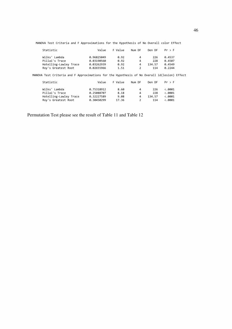
46

MANOVA Test Criteria and F Approximations for the Hypothesis of No Overall color Effect Statistic Value F Value Num DF Den DF Pr > F Wilks' Lambda 0.96825049 0.92 4 226 0.4537 Pillai's Trace 0.03190560 0.92 4 228 0.4507 Hotelling-Lawley Trace 0.03262939 0.92 4 134.57 0.4549 Roy's Greatest Root 0.02655966 1.51 2 114 0.2244 MANOVA Test Criteria and F Approximations for the Hypothesis of No Overall id(lesion) Effect Statistic Value F Value Num DF Den DF Pr > F Wilks' Lambda 0.75318912 8.60 4 226 <.0001 Pillai's Trace 0.25088707 8.18 4 228 <.0001 Hotelling-Lawley Trace 0.32227589 9.08 4 134.57 <.0001 Roy's Greatest Root 0.30450299 17.36 2 114 <.0001

Permutation Test please see the result of Table 11 and Table 12

Documents

The Impact of Midbrain Cauterize Size on Auditory and Visual