Embed Size (px)
Citation preview

ii
THE IMPACT OF INPUT AND OUTPUT MARKET DEVELOPMENT
INTERVENTION OF THE IPMS PROJECT: THE CASE OF MEISO
WOREDA, OROMIYA NATIONAL REGIONAL STATE, ETHIOPIA
A Thesis Submitted to the Department of Agricultural
Economics, School of Graduate Studies
HARAMAYA UNIVERSITY
In Partial Fulfillment of the Requirements for the Degree of
MASTER OF SCIENCE IN AGRICULTURE
(AGRICULTURAL ECONOMICS)
By
TIHITINA ABEBE
June, 2011
Haramaya University

iii
APPROVAL SHEET OF THESIS
SCHOOL OF GRADUATE STUDIES
HARAMAYA UNIVERSITY
As Thesis Research advisor, I hereby certify that I have read and evaluated this thesis
prepared, my guidance, by Tihitina Abebe entitled ―Impact Assessment of Input and
Output Market Development Interventions by IPMS Project: The Case of Mieso
Woreda Oromiya National Regional State, Ethiopia‖. I recommend that it can be
submitted as fulfillment of the Thesis requirement.
Berhanu G/Medhin (PhD) ________________ _______________
Major Advisor Signature Date
Moti Jaleta(PhD) ________________ _______________
Co Advisor Signature Date
As member of the Board of Examiners of the M.Sc. Thesis Open Defense Examination,
we certify that we have read and evaluated the thesis prepared by Tihitina Abebe. We
recommended that the thesis is accepted as fulfilling the Thesis requirement for the Degree
of Master of Science in Agriculture (Agricultural economics).
______________________ _________________ _______________
Chair Person Signature Date
______________________ _________________ _______________
Internal Examiner Signature Date
______________________ _________________ _______________
External Examiner Signature Date

iv
DEDICATION
To my family

v
STATEMENT OF AUTHOR
First, I declare that this thesis is the result of my own work and that all sources or
materials used for this thesis have been duly acknowledged. This thesis is submitted in
partial fulfillment of the requirements for M.Sc. degree at Haramaya University and to be
made available at the university‘s library under the rules of the library. I confidently
declare that this thesis has not been submitted to any other institutions anywhere for the
award of any academic degree, diploma, or certificate.
Brief quotations from this thesis are allowable without special permission, provided that
accurate acknowledgement of source is made. Requests for permission for extended
quotation from or reproduction of this manuscript in whole or in part may be granted by
Dean of the school of graduate studies when in his or her judgment the proposed use of the
material is in the interests of scholarship. In all other instances, however, permission must
be obtained from the author.
Name: Tihitina Abebe Signature: ……………………
Place: Haramaya University, Haramaya
Date of Submission: June, 2011

vi
BIBLIOGRAPHICAL SKETCH
The author was born on 1986 in Haramaya. She attended her primary education at
Haramaya model school and her secondary and preparatory education at SOS Hermann
Gmeiner primary and secondary school in Harar.
She joined Haramaya University in 2004/05 and graduated with B.A. degree in Economics
in 2008.Then she joined the School of Graduate Studies of Haramaya University,
department of agricultural economics in 2008/2009 academic year as a self-sponsored
student for pursuing her MSc degree in agricultural economics.

vii
ACKNOWLEDGEMENTS
First of all, I would like to thank my Lord God for giving me the chance to enjoy the fruits
of my endeavor and giving me courage and endurance to withstand all the problems and
troubles.
Words fail to convey my deepest thanks to my advisor Dr. Berhanu Gebremedhin for his
willingness to advice and guide me with understanding throughout the course of the
research. It is my sublime privilege to express my deepest sense of gratitude and
indebtedness for his scientific guidance and ceaseless support throughout the course of the
research work in addition to restructuring and editing the thesis that is obviously tiresome.
I also remain thankful to my co-advisor Dr. Moti Jaleta.
My deepest overwhelming acknowledgment goes for my parents who have there for me
through everything for their commitments and sacrifices to bring me to this stage. I would
also like to convey my thanks to my entire family for their unforgettable encouragement.
I extend my special thanks to Improving Productivity and Market Success of Ethiopian
farmers‘ project (IPMS) for awarding me graduate fellow position and for financial
support for this study. I am very much grateful to the staff of the pilot learning Woreda‘s
of IPMS, experts and DAs of MoARD, the enumerators.
Finally, I would like to send my gratitude to all individuals and institutions for their
support and encouragement in the entire work of the research.
.

viii
LIST OF ABBREVIATIONS
ADLI Agricultural Development Led Industrialization
AI Artificial Insemination
ATT Average Treatment Effect
CG Consultative Group
CIA Conditional Independence Assumption
CIDA Canadian International Development Agency
CSA Central Statistics Authority
DA Development Agent
DID Difference in Difference
FGD Focus Group Discussion
FTC Farmers Training Center
HH Household
ILRI International Livestock Research Institute
IPMS Improving Productivity through Market Success
M. a. s. l Meters above sea level
MBPRD Mieso Woreda Office of Pastoralists and Rural Development
MoARD Ministry of Agriculture and Rural Development
OCSSCO Oromia Credit and Saving Share Company
PA Peasant Association
PASDEP Plan for Accelerated and Sustained Development to End Poverty
PLW Pilot Learning Woredas
PMG Producer Marketing Groups
PRA Participatory Rural Appraisal
PRSP Poverty Reduction Strategy Program
PSM Propensity Score Matching
SDPRP Sustainable Development and Poverty Reduction Program
SPSS Statistical Package for the Social Sciences
STATA Data Analysis and Statistical Software
STD Standard Deviation
TLU Tropical Livestock Unit
VIF Variance Inflation Factor

ix
TABLE OF CONTENTS
BIBLIOGRAPHICAL SKETCH VI
ACKNOWLEDGEMENTS VII
LIST OF ABBREVIATIONS VIII
TABLE OF CONTENTS IX
LIST OF TABLES XII
LIST OF FIGURES XIII
LIST OF TABLES IN THE APPENDIX XIII
ABSTRACT XIV
1. INTRODUCTION 1
1.1. Background of the Study 1
1.2. Statement of the Problem 4
1.3. Objectives of the Study 5
1.4. Significance of the Study 6
1.5. Scope and Limitations of the Study 6
1.6 Organization of the thesis 7
2. LITERATURE REVIEW 8
2.1. Definition of Basic Concepts 8
2.1.1. Market 8
2.1.2. Marketing 8
2.1.3. Marketing systems 8
2.1.4. Market development 9
2.1.5. Market participation 11
2.2. Agricultural Commercialization 11
2.2.1. Indices in measuring commercialization 12
2.2.2. Determinants and impact of commercialization 15
2.3. Market Imperfection and the Role of Institutions 16

x
TABLE OF CONTENTS (Continued)
2.4. Definition, Types and Approaches of Impact Assessment 18
2.4.1. Types of impact assessment 18
2.4.1.1. Economic impact assessment 19
2.4.1.2. Socio-cultural impact assessment 19
2.4.1.3. Environmental impact assessment 19
2.4.2. Impact assessment approaches 21
2.4.2.1. Experimental method 23
2.4.2.2. Quasi-experimental method 24
2.5. Empirical studies 29
3. RESEARCH METHODOLOGY 32
3.1. Description of the Project 32
3.2. Description of Study Area 34
3.3. Sources and Methods of Data Collection 37
3.4. Sampling Procedures 37
3.5. Methods of Data Analysis 38
3.5.1. Qualitative analysis 38
3.5.2. Descriptive statistics 39
3.5.3. Propensity score matching (PSM) method 39
3.5.2.1. Mathematical specifications of PSM method 41
3.5.2.2. Matching algorithms 47
3.5.2.4. Testing the matching quality 50
3.5.2.5. Estimation of standard error 52
3.5.2.6. Sensitivity analysis 53
3.6. Variable Choice and Definitions 55
3.6.1. Choice and definition of explanatory variables 55
3.6.2. Choice, measurement and indicators of the outcome variables 56

xi
TABLE OF CONTENTS (Continued)
4. RESULT AND DISCUSSION 60
4.1. Description of Sample Households’ Characteristics 60
4.2. Institutional and Organizational Changes of Agricultural Markets in the Woreda
62
4.2.1. Credit facility 62
4.2.2. Agricultural extension service 64
4.2.3. Farmers organization and linkage to different value chain actors 65
4.2.4. Market information service 66
4.3. Empirical Results 66
4.3.1. Propensity scores 67
4.3.2. Matching participant and comparison households 69
4.3.3. Choice of matching algorithm 72
4.3.4. Testing the balance of propensity score and covariates 73
4.3.5. Estimating Treatment Effect on Treated 74
4.3.5.1. Estimates of average treatment effect (ATT) of input use 74
4.3.5.2. Estimates of average treatment effect (ATT) of productivity of onion 75
4.3.5.3. Estimates of average treatment effect (ATT) of net income 76
4.3.5.4. Estimates of average treatment effect (ATT) of marketed surplus 76
4.3.5.5. Estimates of average treatment effect (ATT) of market orientation indicators
77
4.2.4. The sensitivity of the evaluation results 78
5. CONCLUSIONS AND RECOMMENDATIONS 80
5.1. Conclusions 80
5.2. Recommendations 82
6. REFERENCES 84
7. APPENDICES 95

xii
LIST OF TABLES
Table Pages
Table 1: Conceptual frame work in marketing strategies of market development………..10
Table 2: Distribution of Sample of households by type of participation in IPMS project ... 38
Table 3: Type, definitions and measurement of variables ..................................................... 56
Table 4: Descriptive statistics of sample households (continuous variables)…………….61
Table 5: Descriptive statistics of sample households (Dummy variables) ........................... 62
Table 6: Access to formal credit…………………………………………………………63
Table 7: Reason for not taking credit…………………………………………………..63
Table 8: Source of credit ………………………………………………………………..64
Table 9: Extension service………………………………………………………………65
Table 10: Membership to formal organization……………………………………………66
Table 11: Logit results household program participation ...................................................... 68
Table 12: Distribution of estimated propensity scores ........................................................... 70
Table 13: Performance of matching estimators ...................................................................... 72
Table 14: Balancing test of each covariates using t-test ........................................................ 70
Table 15: Chi-square test for the joint significance of variables ........................................... 74
Table 16: Estimation of ATT: Impact of IPMS program on input intensity......................... 75
Table 17: Estimation of ATT: Impact of IPMS program on productivity of onion ............ 75
Table 18: Estimation of ATT: Impact of IPMS program on net income .............................. 76
Table 19: Estimation of ATT: Impact of IPMS program on market surplus ....................... 77
Table 20: Estimation of ATT: Impact of IPMS program on market orientation .................. 78
Table 21: Sensitivity analysis of the estimated ATT……………………………………79

xiii
LIST OF FIGURES
Figure Page
Figure 1: Location of the study area ........................................................................................ 36
Figure 2: Kernel density of propensity score distribution ...................................................... 69
Figure 3: Kernel density of propensity scores of participant households ............................. 71
Figure 4: Kernel density of propensity scores of non participant households ...................... 71

xiii
LIST OF TABLES IN THE APPENDIX
Appendix Table page
1. Multicollinearity test for continuous explanatory variables...................................... 96
2. Contingency coefficient for discrete variables ......................................................... 96
3. Conversion factor used to calculate TLU.................................................................. 96
4. Conversion factor for adult equivalent (AE)………………………………………..97
4. Histogram of Pscore with common (off) support regions ....................................... 97

xiv
IMPACT ASSESSMENT OF INPUT AND OUTPUT MARKET DEVELOPMENT
INTERVENTIONS OF THE IPMS PROJECT: THE CASE OF MIESO WOREDA,
OROMIYA NATIONAL REGIONAL STATE, ETHIOPIA
ABSTRACT
Improving Productivity and Market Success of Ethiopian farmers’ (IPMS) is a project that
is being implemented by ILRI at 10 pilot learning woredas in the country to enhance
market oriented production so that the country can overcome the problems of poorly
developed agricultural production and marketing. Even though the project has been in
place for over five years its impact has not been evaluated. Therefore, this study evaluates
the impact of input and output market development interventions of the project on
institutional and organizational aspect of markets, input use and productivity, total net
income, marketed surplus and market orientation of the participant households. For
quantitative analysis both program participant and non participant respondents were
drawn and cross-sectional survey data were collected from 180 households in Mieso
woreda. A propensity score matching method was applied to assess the impact of the
project on outcome variables of the treated households. Results show that the market
development interventions have a significant and positive impact on the outcome variables
measured using different indicators. The intervention has resulted in positive and
significant impact on level of input use for onion and goat production of the treated
households. Participants earned more total net income on average from commodities of
intervention over non-participants and also found to be more market oriented and
supplied more of their produce to market over non-participants. However, some outcome
variable indicators such as input use for cattle, net income from goat, land allocated for
onion and proportion of goat allocated for fattening by participant households are
positive but statistically insignificant. The sensitivity analysis also show that results are
not sensitive to unobserved selection bias and were robust to the dummy cofounder. These
results reveal that market development interventions of such kind play an important role
for the overall transformation and development activities of the country.
Key words: Input and output market development intervention, propensity score matching,
Mieso, impact.

1
1. INTRODUCTION
1.1. Background of the Study
Agriculture is the mainstay of the Ethiopian economy. The agricultural sector accounts for
45 percent of national GDP, 83.9 percent of export earnings and 85 percent of
employment opportunity (CIA, 2010). Ethiopia has reasonably good resource potential for
agricultural development. Despite agricultural sector‘s importance in the livelihood of the
people and its potential, the sector has still remained at subsistence level due to
multifaceted problems (Dercon and Zeitlin, 2009). As a result, Ethiopia is faced with
broad, deep and structural poverty problem.
The prevalence of poverty in Ethiopia is associated with slow growth and low productivity
of subsistence agriculture. Low productivity in turn is associated among others with very
low technical progress. The dependence on rain-fed cultivation practice renders the
economy vulnerable to the vagaries of weather conditions (IPMS, 2005).
Like in many developing countries, poverty, food insecurity and poor nutrition were the
country‘s endemic social and economic problems for most of the second half of the 20th
century especially among the rural population predominantly dependent on low productive
subsistence farming. Consequently, in the first decade of the 21st century they still remain
as central policy concern to the Government of Ethiopia. In spite of tremendous efforts,
Ethiopia is still among the poorest developing countries with an annual average per capita
income of US$317 in 2008 (UNDP, 2010). Furthermore, around 38.7% of the country‘s
populations are below the national poverty line in 2009 (CIA, 2010).
In view of these state of affairs, right from its seizure of power, the current Government of
Ethiopia has formulated policies and strategies to guide overall economic development
with focus on rural and agricultural development. The fundamental development objective
of building a free-market economic system in the country is expected to facilitate
economic development, and extricate the country from dependence on food aid and reduce
poverty.

2
These policies and strategies mainly focus on bringing about a structural transformation in
agricultural sector and a shift from subsistence production to market-oriented production.
They carried important strategic direction in relation to infrastructure, human
development, rural development, food security, and capacity-building. They also
recommended specialization both at farm and commodity level, a shift to a high-value
crops, promotion of niche high-value export crops and a stronger focus on selected high-
potential areas. In fact, they also embodied some bold new directions by giving high
policy attentions to greater commercialization of agriculture and enhancing private sector
development, industry, increased availability and utilization of appropriate technologies,
an effective and efficient service delivery system, improving institutional competence and
performance, urban development and a scaling-up of efforts to achieve the Millennium
Development Goals (MDGs)1.
The performance of the agricultural sector has been the base for economic growth in
Ethiopia. However, Ethiopian agriculture as well as the agricultural marketing has been
poorly developed. Nevertheless efficient agricultural marketing system is the main driving
force for successful agricultural development and the economy in general. Inefficient
performance of the agricultural markets in Ethiopia has been known in various studies as a
major hindrance to growth in the agricultural sector and the overall economy. If the
marketing system is inefficient, high marketing costs will render products uncompetitive
particularly on the international market (MOFED, 2002). Moreover, poorly-functioning
credit, input, and product markets may prevent asset-poor farmers from being able to
exploit the higher returns to available land and labor that increased agricultural
commercialization may provide (Jayne et al., 1994). Thus, improving the efficiency of
markets is an important part of the overall development strategy.
In order to attain economic development in Ethiopia the current subsistence oriented
agricultural production system needs to be transformed into a market oriented production
system. Hence, the government has emphasized the transformation of subsistence
1 Millennium Development Goals (MDGs) are those goals set to: eradicate poverty and hunger, achieve
universal primary education, promote gender equality and empower women, reduce child mortality, improve
maternal health, combat HIV/AIDS, malaria and other diseases, ensure environmental sustainability, develop
a global partnership for development.

3
agriculture into market orientation as a basis for long-term development of the agricultural
sector. To be competent both at the local and international markets, a focus should be
given to farm level production efficiency, product quality, post harvest handling and
technologies. As opposed to producing for subsistence, producing primarily for the market
(both domestic and export markets), quality and standard of the produce become much
more important, since competitiveness depends partly on quality of produce which in turn
depends heavily on the use of the right technologies and methods of production. Rapid
adjustments in production technologies and timely and effective transmission of market
information are vital in altering market conditions and consumer preferences.
Standardization of agricultural products, improving the supply of market information
system, expanding and strengthening cooperatives, and strengthening private sector
participation are key elements for proper functioning of the agriculture marketing
system(MOFED, 2002).
It is with this background that, the Improving Productivity and Market Success (IPMS)
project was formulated and has been implemented since 2005. IPMS is donor-supported
and implemented by the International Livestock Research Institute (ILRI) on behalf of the
Ministry of Agriculture of the Federal Democratic Republic of Ethiopia (MoA). The
project follows a value chain development approach, which is made up of several
interconnected components that include input supply and services, production, post
harvest management and processing, distribution and marketing and consumption (IPMS,
2005). Key to such development is to create the capacity of the rural communities, where
farmers produce what they can market rather than trying to sell what they already produce.
The main objective of the project is to contribute to a reduction in poverty of the rural poor
through market oriented agricultural development. In attaining this objective, the project
supported development and research on innovative technologies, processes and
institutional arrangements in the following four focus areas: knowledge management;
innovation capacity building of public and private sector partners, farmers and pastoralists;
participatory marketable commodity development and development and promotion of
recommendations for scaling out (IPMS, 2005).

4
The project has been implemented in 10 pilot woredas (PLWs) in four major Regional
States in the country. In view of helping farmers to improve farm productivity and their
market orientation, the project has been assisting the government by accelerating the
introduction of technology and institutional innovations, in collaboration with relevant
stakeholders so that the technology adoption and application process is enhanced.
However, no study has been conducted in assessing the impact of the interventions of the
IPMS project in one of the PLWs, Mieso woreda in Western Hararghe. An assessment of
the impact of the market oriented interventions would be useful to draw lesson for scaling
out and up of successful interventions. This study is, therefore, aimed at evaluating the
impact of the interventions of the IPMS project in Mieso Woreda and aimed at filling the
existing knowledge gap.
1.2. Statement of the Problem
Many rural families in Ethiopia suffer from chronic food insecurity and are extremely
vulnerable during periodic drought. The methods and techniques of agricultural production
and distribution are traditional and result in low productivity (IPMS, 2005). Limited
resource ownership, low levels of adoption and use of improved technologies and lack of
adequate infrastructure and institutions that support agricultural development are the major
factors behind low productivity of small scale agriculture in Ethiopia.
The level and speed of economic development in Ethiopia is heavily influenced by
sustained growth in agriculture. Sustained agricultural growth requires increased
availability of technologies, farm inputs and services on the one hand and sustained
demand for agricultural output on the other. Agricultural marketing is the main driving
force for economic development and has a guiding and stimulating impact on production
and distribution of agricultural production. However, agricultural markets are inefficient in
Ethiopia.
It is increasingly recognized that the commercialization of small-scale farming is closely
linked to higher productivity, greater specialization, and higher income (Timmer, 1997).
Furthermore, in a world of efficient markets, commercialization leads to the separation of

5
households‘ production decisions from their consumption decisions, supporting
specialization at household level and diversification at regional or national level. At the
macro level, commercialization has also been shown to increase food security and, more
generally, to improve allocative efficiency (Timmer, 1997; Fafchamps, 2005).
The IPMS project which aims at contributing to reduction of poverty of the rural poor
through market-oriented agricultural development has been implemented in Mieso woreda
since 2004. Linking producers to the potential buyers and input suppliers,
developing/strengthing producers‘ cooperatives, establishing alternative input shops,
involving private sector in input and output marketing were some of the interventions
made in the market development component of the project for the selected market oriented
commodities: onion; goat and cattle. However, the impact of these interventions has not
been assessed.
Evaluating impact is particularly critical in developing countries where resources are
scarce and every dollar spent should aim to maximize its impact on poverty reduction. It
has greater importance for the economical allocation of scarce resources in addition to its
importance in providing evidence for governments, aid donors and development
communities, who are increasingly asking for hard evidence on the impact of public
spending projects claiming to reduce poverty.
Hence, this study attempts to provide empirical evidence on the impact of IPMS
interventions on institutional and organizational setups of the woreda market, marketed
surplus, total household net income, farm intensification and productivity, and households‘
market orientation behavior for the market oriented commodities of interventions in the
Mieso woreda.
1.3. Objectives of the Study
The general objective of the study is to assess the impact of input and output market
development interventions by IPMS project on change on institutional and organizational
aspect of markets, input intensity and productivity, net income, market surplus and market
orientation of households.

6
The specific objectives are: to:
1. Describe the changes in the organizational and institutional aspects of agricultural
markets due to the intervention;
2. Measure the impact of the market interventions on livestock (goat and cattle) and
onion intensification and productivity;
3. Measure the impact of the interventions on household net total income from onion
and goat and cattle fattening;
4. Measure the impact of the interventions on marketed surplus of onion and fattened
goat and cattle; and
5. Measure the impact of the market interventions on market orientation of onion
producing and goat and cattle fattening households.
1.4. Significance of the Study
In countries like Ethiopia where investment capital is very limited, knowing the impact of
project interventions is critical. Hence, assessing the impact of IPMS towards increased
agricultural productivity and market success of Ethiopian farmers would be important to
all stakeholders (beneficiaries, MoA and donors and also other rural development actors
aiming at formulating and implementing similar projects). These stakeholders need to
know the impact in order to draw lesson to improve project design and intervention
implementation. Such impact assessment study is especially important for scaling out and
up of success stories to achieve greater impact at larger scale. Evidence based project
planning and implementation would save scarce funds from being used unwisely
1.5. Scope and Limitations of the Study
The study was undertaken in Mieso woreda of Oromia National Regional State with the
main intention of assessing the impact of input and output market development
interventions of IPMS on different outcomes of interest. The study was limited to the
impact of market development interventions only for onion production and goat and cattle
fattening undertaken in the woreda with the support of the project. Hence, confinement to
one woreda and focus only on a few commodities may limit the generalization of the

7
results. However, it is believed that the results would shed a strong clue on the direction of
impact of the overall project intervention since the three commodities were the major
focus of the interventions. Since Mieso woreda is the only pastoral/agro pastoral woreda
of the IPMS PLWs, the study is useful in terms of drawing lessons to similar farming
systems in Ethiopia.
1.6 Organization of the thesis
This thesis is organized in five chapters. Chapter one presents the introductory part of the
study. The following chapter presents literature review that includes concepts on market,
market development, market participation, market orientation and their measurements and
linkage of institutions and marketing and impact evaluation methods. Chapter three
introduces the methodology which includes description of the program and study area,
source and methods data collection and analysis as well. Chapter four describes the results
and discussion of the research outcomes and finally chapter five summarizes the findings
of the study and draws appropriate conclusions and policy implication.

8
2. LITERATURE REVIEW
2.1. Definition of Basic Concepts
2.1.1. Market
The word ―market‖ has been defined differently by different scholars over the years. Some
of these definitions are as follows. One old definition states that market is another name
for demand (McNair and Hansen, 1956). Alternatively, market is defined as a single
arrangement in which one thing is exchanged for another (Bain and Howells, 1988). A
market is also thought of as a meeting point of buyers and sellers: a place where sellers
and buyers meet and exchange takes place: an area for which there is a demand for goods
and area for which price determining forces (demand and supply) operate. Moreover, in
modern times a market is also defined as an arena for organizing and facilitating business
activities and for answering the basic economic questions like how much to produce?
What to produce? How to distribute production? (Kohls and Uhl, 1985). As a result, one
can understand that the word market has a concept of location, product, time, demand and
a group of consumers and suppliers.
2.1.2. Marketing
Another basic concept that is closely related to market is marketing. There is no
universally accepted definition of marketing since the usefulness and validity of a
definition is associated with its application. For this study, the following definition was
used. ‗Marketing is the performance of all business activities involved in the flow of goods
and services from the point of initial agricultural production until they are in the hands of
ultimate consumers‘ (Kohl, 1968 cited in Jone, 1972).
2.1.3. Marketing systems
A marketing system is a collection of actors, channels, intermediaries, business activities,
and institutions which facilitate the physical distribution and economic exchange of goods
(Kohls and Uhl, 1985). A marketing system can also be regarded as a multi-layered

9
sequence of physical activities and of transfers of property rights from the farm-gate to the
consumer (White, 1995). A channel of distribution may be defined as a path traced in the
direct or indirect transfer of the title to a product as it moves from a producer to ultimate
consumer or industrial users.
2.1.4. Market development
Market development is a process for developing sales – new business and new markets.
This process is effective for developing all types of business, and delivers business growth
via: new products or services to existing customers, existing products or services to new
customers, or new products or services to new customers (Chapman, 2009).
It can also be said that market is developed, if in addition to the existing markets, new
markets are created like niches and linkage to supermarkets which has not been practiced
before though marketing practice has been there for long periods, new customers are
targeted, different institutions and organizations are involved in every activities in the
value chain development approach (Mwape, 2009). In this regard, improving quality and
quantity of the existing product, targeted marketing strategies are important components.
Market development may include identifying the products which have potential demand in
the domestic as well as international market places, linking potential buyers and sellers,
provision of market information which contributes for reduction in marketing costs,
establishing primary cooperatives in order to improve their bargaining power and further
reduce the transaction costs in the value chain approach (Mwape, 2009).
An important framework for market development is that developed by Ansoff (1957)
which classifies market development into market penetration, product development,
market development and diversification.

10
Table 1: Conceptual framework in marketing strategies of market development
Existing products New products
Existing markets Market penetration Product development
Increase sales of products to existing
market segments e.g decrease
prices, promotion
Identify opportunities for new
or modified
products e.g. product
differentiation
through new packaging,
brands, additional processing,
quality improvement
New markets Market development Diversification
Expanding into new
geographical area,
selling to new segments
of the population, New
product dimensions or
packaging etc.
Identify opportunities for new
products
for new clients or markets
Source: Adopted from Ansoff (1957)
According to Ansoff (1957), the main components of market development are: marketing
extension and training; market information and intelligence network; grading and
standardization at producer‘s level; improvement in competition and awareness;
accessibility of marketing finance and credit; and promoting the product by targeting
different customers.
Similarly, Eleni and Goggin (2006), explain that market development requires an
integrated rather than piecemeal approach, in which the key market institutions needed,
such as market information, grades and standards, contract enforcement, regulation, and
trade and producer groups, involvement of different stakeholders are integrated. Moreover,
the interaction of these stakeholders and the institutions which are governing them are
very important for the best functioning of the activities.
Input and output marketing system play key roles in the adoption of agricultural
technologies. If farmers do not have efficient input and output markets, they resist
investing in new and more productive technologies (Oechmke et al., 1997). Thus,
generally it can be said that, market development increases the competitiveness of selected
agricultural sub-sectors that target national, sub-regional and international markets thereby
contributing to agricultural growth.

11
2.1.5. Market participation
William et al. (2008) defined market participation in terms of sales as a fraction of total
output, for the sum of all agricultural crop production in the household which includes
annuals and perennials, locally-processed and industrial crops, fruits and agro-forestry.
This sales index would be zero for a household that sells nothing, and could be greater
than unity for households that add value to their crop production via further processing
and/or storage.
Market participation is both a cause and a consequence of economic development.
Markets offer households the opportunity to specialize according to comparative
advantage and thereby enjoy welfare gains from trade. Recognition of the potential of
markets as engines of economic development and structural transformation gave rise to a
market-led paradigm of agricultural development (Reardon and Timmer, 2005).
Improvements in market participation are necessary to link smallholder farmers to markets
in order to expand demand for agricultural products as well as set opportunities for income
generation (Pingali, 1997). Market-orientation enhances consumers‘ purchasing power for
food, while enabling re-allocation of household incomes by producers to high-value
nonfood agribusiness sectors and off-farm enterprises (Davis, 2006). Specific
opportunities exist in non-trade distorting measures such as irrigation, intensification,
extension and input supply. In addition, niche markets for differentiated products,
contracts with village-level institutions (e.g., schools, hotels), and investments in value
addition are areas where smallholder farmers would considerably benefit if challenges to
their effective participation were addressed (Omiti et al., 2007). The rationale for
enhancing participation in commercial agriculture also stems from the potential to
accelerate attainment of the Millennium Development Goals on food security and poverty
reduction through utilization of untapped opportunities in commodity value chains
(MOFED, 2006).
2.2. Agricultural Commercialization
In a broad sense, smallholder commercialization could be seen as the strength of the
linkage between farm households and markets at a given point in time. This household-to-

12
market linkage could relate to output or input markets either in selling, buying or both.
Alternatively, smallholder commercialization could also be seen as a dynamic process: at
what speed the proportion of outputs sold and inputs purchased are changing over time at
household level.
In most literature, a farm household is assumed to be commercialized if it is producing a
significant amount of cash commodities, allocating a proportion of its resources to
marketable commodities, or selling a considerable proportion of its agricultural outputs
(Immink and Alarcon, 1993; Strasberg et al., 1999). However, the meaning of
commercialization goes beyond supplying surplus products to markets (von Braun et al.,
1994; Pingali 1997). According to these authors, it has to consider both the input and
output sides of production, and the decision-making behavior of farm households in
production and marketing simultaneously. Moreover, commercialization is not restricted
only to cash crops as traditional food crops are also frequently marketed to a considerable
extent (von Braun et al., 1994; Gabre-Madhin et al., 2007). Commodities traditionally
considered as food crops may increasingly be marketed during the transformation process
as households specialize.
The commonly accepted concept of commercialization is, therefore, that commercialized
households are targeting markets in their production decisions, rather than being related
simply to the amount of product they would likely sell due to surplus production (Pingali
and Rosegrant, 1995). In other words, production decisions of commercialized farmers are
based on market signals and comparative advantages, whereas those of subsistence
farmers are based on production feasibility and subsistence requirements, and selling only
whatever surplus product is left after household consumption requirements are met.
(Pingali and Rosegrant, 1995; Berhanu and Dirk, 2009). Depending on the various
literatures commercialization can be generalized as households‘ production decision
targeting markets rather than production for subsistence requirements.
2.2.1. Indices in measuring commercialization
The relevance of measuring the level of smallholder commercialization arises from the
interest to make comparisons of households according to their degree of
commercialization (Randolph, 1992). In addition, it also helps to gauge to what extent a

13
given farm household is commercialized in its overall production, marketing and
consumption decisions, and to analyze the determinants of commercialization. However,
there are diverse methods or indicators used for measuring the level of commercialization.
Focusing on commercialization in its static form, various authors have used different
yardsticks in measuring the level of agricultural commercialization at household level.
Von Braun et al., (1994) specified three types of commercialization indices at household
level: output and input side commercialization, commercialization of the rural economy,
and degree of a household‘s integration into the cash economy. For each type, the authors
formulated indices measuring the extent of household commercialization. The first index
measures proportion of agricultural output sold to the market and input acquired from
market to the total value of agricultural production. In the second type, commercialization
of the rural economy is defined as the ratio of the value of goods and services acquired
through market transactions to total household income. Here, there is an assumption that
some transactions may take place in-kind such as payments with food commodities for
land use. Thirdly, the degree of household integration to the cash economy is measured as
the ratio of the value of goods and services acquired by cash transaction to the total
household income.
In measuring household-specific level of commercialization, Govereh et al., (1999) and
Strasberg et al., (1999) used a household commercialization index (HCI), which is a ratio
of the gross value of all crop sales per household per year to the gross value of all crop
production. This ratio does not incorporate the livestock subsector, which could be more
important than crops in some farming systems (Moti et al., 2009).
Recently, Gabre-Madhin et al., (2007) used four approaches to measure the level of
household commercialization: sales-to-output and sales-to-income ratios, net and absolute
market positions (either as a net buyer, net seller or autarkic/self-sufficient household),
and income diversification or level of specialization in agricultural production.
According to Gabre-Madhin et al., (2007), the sales-to-output ratio measures the gross
value of all agricultural sales by a household as a percentage of the total gross value of its
agricultural production. The total sales-to-income ratio is the ratio of the gross value of
total sales to total income from crop production. In this index, income from crop
production is assumed as a proxy to total household income, ignoring income from

14
livestock, and off- farm and non-farm sources. The market position of a household is
evaluated using the ratio of volume of sales and volume of purchases to the total volume
of stock: the sum of storage from the previous production year and production in the
current year. The specialization index tries to capture to what extent farm households are
specialized in their production to capture the benefits from comparative advantages:
producing what they can efficiently produce and buying what they cannot. This index
measures the proportion of the value of purchased agricultural products not produced by
households to the gross value of agricultural production.
In addition to the above indices, von Braun et al. (1994) have measured commercialization
in terms of proportion of land allocated by farmers to commercial crops and in terms of
the value of input and output sales and purchases weighted by the value of agricultural
production.
In most literature, the issue of commercialization is based on the proportion of resources
allocated to either cash or food crops. However, under the existence of favorable market
environment and infrastructure, food crops could also have the potential to be commercial
crops (Fafchamps, 1992). Moreover, cash crops are not necessarily supplied to the market.
Therefore, categorizing crops broadly into food and cash crops to analyze the extent of
household commercialization lacks a strong footing and requires looking at the purpose
for which a crop is grown rather than looking at the nature/type of crop itself.
Based on this review, it appears that the common approach to measuring the degree of
smallholder commercialization is based on the proportion of the value of agricultural
produce sold or the value of agricultural inputs bought to the total household agricultural
income (Randolph 1992; von Braun et al., 1994).
With the aim to identify the position of a farm household in livestock market participation,
Asfaw and Jabbar (2008) formulated a gross and net (market) livestock off-take rates at
the household level. The gross off-take rate measures the overall rate of inventory changes
of livestock in a household. It categorizes births, gifts received, and purchases as incoming
animals whereas deaths, sales, gifts, and slaughters are considered as outgoing ones. The
gross off-take rate is then defined as the ratio of the difference of the two to the average
inventory of a given period (usually one year). The net (market) off-take rate, which is
15
more relevant in measuring the level of smallholder commercialization, considers only the
sales and purchases of livestock per household per a specific period. Net off-take rate is
then computed as the ratio of the difference of the two to the average inventory of the
period.
2.2.2. Determinants and impact of commercialization
There are a number of determinants in commercialization of smallholder agriculture.
These determinants are broadly categorized as external and internal factors. The external
ones are factors beyond the smallholder‘s control like population growth and demographic
change, technological change and introduction of new commodities, development of
infrastructure and market institutions, development of the non-farm sector and the broader
economy, rising labor opportunity costs, macroeconomic, trade and sectoral policies
affecting prices and other driving forces (von Braun et al., 1994; Pingali and Rosegrant,
1995).
In addition, development of input and output markets, institutions like property rights and
land tenure, market regulations, cultural and social factors affecting consumption
preferences, production and market opportunities and constraints, agro-climatic
conditions, and production and market related risks are other external factors that could
affect the commercialization process (Pender et al., 2006). On the other hand, factors like
smallholder resource endowments including land and other natural capital, labor, physical
capital, human capital etc. are household specific and are considered to be internal
determinants.
Impacts of commercialization can be categorized into first, second and third orders (Moti
et al., 2009). The first-order is mainly income and employment effects that are directly
reflected in household welfare. The second-order effects include health and nutrition
aspects usually contingent on the level of income attained through the existing level of
commercialization. The third-order (or usually known as higher order) effects are the
macro-economic and environmental effects that go beyond household level.
Agricultural commercialization tends to generate more household income due to its
comparative advantages over subsistence production (Kennedy and Cogill 1987; Dorsey

16
1999). However, unless rural markets are well-integrated and risks are low to influence
household decision behavior, the shift from subsistence to commercial production may
have an adverse consequence by exposing households to volatile food market prices and
food insecurity.
2.3. Market Imperfection and the Role of Institutions
Institutions are defined in many different ways. The most widely quoted definition is the
one given by North (1990) which defines institutions as humanly devised, made up of
formal constraints (i.e., rules, laws, constitutions), informal constraints (i.e., norms of
behavior, conventions and self-imposed codes of conduct) that structure human
interactions, and their enforcement characteristics. These constraints and the technology
employed determine the transaction and transformation costs that add up to the production
and marketing costs.
North (1990), and Dorward et al., (2005) define institutions as ―rules of the game‖ that
define the incentives and sanctions affecting people‘s behavior and distinguish
institutional arrangement as sets of rules and structures that govern particular contracts,
and the context within which the contracts are governed. The World Bank (2002) offers a
working definition of market institutions as rules, enforcement mechanisms and
organizations that promote market transactions. These definitions indicate that institutions
provide multiple functions to markets; they transmit information, mediate transactions,
facilitate the transfer and enforcement of property rights and contracts, and manage the
degree of competition. Along with these definitions, we define market institutions as rules
of the game, enforcement mechanisms and organizations that facilitate market interaction,
coordination, contract formation and enforcement.
Market failures are caused by asymmetric information, high transaction costs and
imperfectly specified property rights. Where supporting market institutions are lacking,
rural markets in areas with low market infrastructure tend to be very thin, imperfect or
missing. In the absence of institutions that help to coordinate marketing functions or to
link producers to markets, the associated high transportation costs and transaction costs
undermine the processes of exchange and result in limited or localized markets with little
rural-urban linkages (Kranton, 1996; Eleni, 2001; Chowdhury et al., 2005). In such

17
circumstances, households produce only a limited range of goods and services for their
own consumption because social protection for food security is not provided through
markets and government interventions (de Janvry et al., 1991).
When high transaction costs, asymmetric information and incomplete property rights
impede the functioning of markets, market players fail to undertake profitable investments
(due to the absence of complementary investments) leading to coordination failures that
hinder market functions (Dorward et al., 2003, 2005, Poulton et al., 2006). Thus,
coordination failure along the production-to-consumption value chain may explain
constrained agricultural development and the prevalence of a low equilibrium trap, which
is a big challenge to policy (Dorward et al., 2003). Overcoming the effects of such market
imperfections in agricultural input and output markets would therefore require a deliberate
attempt to strengthen institutions that promote coordination of market functions, reduce
transaction costs and integrate markets to facilitate a continual transition to a higher level
equilibrium (World Bank, 2002).
Various private and public sector market-supporting institutions and institutional
arrangements have been proposed to bridge market imperfections, reduce transaction
costs, enhance opportunities for the poor in markets and to make the market systems more
inclusive and integrated (World Bank, 2002). Among the potential market-supporting
institutions that can enhance market functions in rural areas are farmer organizations such
as Producer Marketing Groups (PMGs). Their potential in this process lies in enabling
contractual links to input and output markets; promoting economic coordination in
liberalized markets and in leveraging market functions for smallholder farmers. However,
their success in this process depends on their ability in conveying market information;
coordinating marketing functions; defining and enforcing property rights and contracts;
facilitating smallholder competitiveness in markets, and more critically in mobilizing their
members to engage in markets. (Rondot and Collion, 1999; Coulter et al., 1999; World
Bank, 2002)

18
2.4. Definition, Types and Approaches of Impact Assessment
Impact refers to the broad, long-term economic, social and environmental effects that may
be anticipated or unanticipated, and positive or negative, at the level of the individual or
the organization. Such effects generally involve changes in both cognition and behavior
(Omoto, 2003). Impact evaluations are not simply about measuring whether a given
program is having a positive effect on participants.
An impact evaluation also assesses the extent to which a program has caused desired
changes in the intended audience. It is concerned with the net impact of an intervention on
households and institutions, attributable only and exclusively to that intervention. Thus,
impact evaluation consists of assessing outcomes and, thus, the short or medium-term
developmental change resulting from an intervention (Baker, 2000).
Impact evaluation is aimed at providing feedback to help improve the design of programs
and policies. In addition to providing for improved accountability, impact evaluations are
a tool for dynamic learning, allowing policymakers to improve ongoing programs and
ultimately better allocate funds across programs. There are other types of program
assessments including organizational reviews and process monitoring, but these do not
estimate the magnitude of effects with clear causation. Such a causal analysis is essential
for understanding the relative role of alternative interventions in reducing poverty.
2.4.1. Types of impact assessment
People level impact refers to the effect of the technology or intervention on the ultimate
users or target group for which the technology was developed. Impact begins to occur
when there is a behavioral change among the potential users. The people level impact
deals with the actual adoption of the intervention output and subsequent effects on
economic, socio-cultural, and/or environmental conditions of beneficiaries (Omoto, 2003).

19
2.4.1.1. Economic impact assessment
Economic impact measures the combined production and income effects associated with a
set of research and development activities. The economic impact can be assessed through
what is known as an ―efficiency analysis‖ which compares the cost and the benefits of the
project in a systematic manner (Anandajayasekeram et al., 1997). The economic impact
assessment studies range in scope and depth of evaluation from partial impact studies to
comprehensive assessment of economic impacts. One popular type of partial impact
assessment is adoption studies that look at the effects of new technology such as the
spread of modern plant varieties on farm productivity and farmers‘ welfare. Economic
impact assessments of the more comprehensive types look beyond mere yield and crop
intensities to the wider economic effects of the adoption of new technology. The literature
on economic impact studies also includes a wide range of levels of impact analysis, from
aggregate, national level to program and project level.
2.4.1.2. Socio-cultural impact assessment
Socio-cultural impacts assessment (SIA) include the effects of a project on the attitude,
beliefs, resource distribution, status of women, income distribution, nutritional
implications, institutional implications etc of the community. These can be assessed
through socio-economic surveys and careful monitoring. SIA as a process and
methodology has the potential to contribute greatly to the planning process of other types
of development projects (Burdge and Vanclay, 1996). It can assist in the process of
evaluation of alternatives projects/programs, and to help in their understanding and
management of the process of social change. Social impacts are important and need to be
considered along with the economic and environmental impacts. SIA can enrich the
impact analysis as well as provide a clearer identification of issues for project planning
and prioritization.
2.4.1.3. Environmental impact assessment
Environmental Impact Assessment (EIA) is defined as the process of identifying,
predicting, evaluating and mitigating the biophysical, social, and other relevant effects of

20
development activities prior and/or subsequent to major decisions being taken and
commitments made (IAIA, 1998). Many countries require (EIAs) for major development
projects; and, in fact, many countries have formal requirements in law and associated
guidelines for carrying out EIAs. The importance of EIA is increasing in agricultural
research and development due to the growing concerns of land degradation, deforestation
and loss of biodiversity around the world. However, there are few examples of countries
and research institutions that have formally assessed the environmental impacts associated
with agricultural research and development projects. Environmental costs and benefits are
typically not included in conventional economic impact studies. Among other things, there
is a clear lack of adequate data on which to base EIA (Alston et al., 1998).
2.4.1.4. Institutional impact assessment
Institutional impact consists of changes in organizational structures, methods of
conducting scientific research and development activities, and the availability and
allocation of research resources (Omoto, 2003). Most of the ongoing research and
development impact studies address the people level impact forgetting institutional
impacts. Increasing agricultural productivity, whilst strengthening local institutions, has
long been an important goal of agricultural research and development activities.
Organizations play an important role in meeting this goal by improving technologies and
knowledge base of the biological, social, economic and political factors that govern the
performance of an agricultural system, and by strengthening local institutions‘ capacity
and performance. Institutional impact assessment involves the evaluation of the
performance of organizations in non-technological research activities such as training,
networking, development of methodologies, and advisory services in the areas of research
and other policies, organization and management (Omoto, 2003). Assessment of the
institutional impacts of such activities should therefore be an integral part of the overall
impact assessment and research evaluation efforts.
There has been little methodological and practical work in the area of institutional impact
assessment of agricultural research and development interventions (Goldsmith, 1993).
This includes the impact an agricultural research organization has on capacity building,
human resources development, and performance of other institutions. However, recently
there has been growing interest to evaluate the institutional impacts. Institutional and

21
organizational impact is measured in terms of changes in policy, institutional structure,
networking, arrangements and achievements in human capacity buildings, human resource
development and performance of other institutions (Omoto, 2003).
The concrete results and impacts of institutional development can be difficult to see and
may take time to emerge. However, information generated from institutional impact
assessment has the great potential to lead to better, more effective actions and institutional
performance of development intervention and research system.
Impact assessments can be classified into ex ante impact assessment and ex post impact
assessment. Ex ante evaluations are undertaken before the project or program is initiated
as an aid in priority setting (Mywish et al., 2003). Ex ante impact studies are conducted to
estimate the expected returns from current alternative projects/programs. Assessment of
future impact includes measures of productivity impacts, distribution of economic
benefits, and effects on environmental quality. And ex post evaluations are undertaken
after diffusion of a research product has been initiated or a certain project or program has
been implemented, to assess actual impacts on the ground. However, ex post evaluations
generate information that is useful for the selection, planning and management of future
programs, such as plausible adoption paths. Ex post impact assessment develops the
confidence of scientists, research managers, and stakeholders and makes the case for
enhanced support (Bantilan and Dar, 2001).
The impact assessment process becomes complete when adoption and impact information
obtained from ex post impact studies is fed back to ex ante impact studies and the process
continues, as technology development itself is continuous. Such evaluations may provide
decision makers with pertinent information but their lack of rigor often undermines their
credibility, especially in today‘s climate of accountability (Mywish et al., 2003).
2.4.2. Impact assessment approaches
In order to determine the effects of the intervention, it is necessary to identify what would
have happened without the intervention. What would have been the welfare levels of
particular communities, groups, households and individuals without the intervention?
Evaluation involves an analysis of cause and effect in order to identify impacts that can be

22
traced back to interventions (Ezemenari et al., 1999). These questions cannot, however, be
simply measured by the impact of a project. There may be other factors or events that are
correlated with the impact but are not caused by the project. To ensure methodological
rigor, an impact evaluation must estimate the counterfactual, that is, what would have
happened had the project never taken place or what otherwise would have been true.
However, the two situations cannot be observed for the same individual. In other words,
only the factual situation can be observed. Thus, the fundamental problem in any social
program evaluation is the missing data problem (Bryson et al., 2002; Ravallion, 2005).
To determine the counterfactual, it is necessary to net out the effect of the interventions
from other factors—a somewhat complex task. This is accomplished through the use of
comparison or control groups (those who do not participate in a program or receive
benefits), which are subsequently compared with the treatment group (individuals who do
receive the intervention). Determining the counterfactual is at the core of evaluation
design and a key to identifying what would have occurred in the absence of the
intervention (Ezemenari et al., 1999). However, this is difficult to achieve for two reasons.
First, beneficiaries of the intervention may be selected on the basis of certain
characteristics (purposive targeting). If these characteristics are observed then a
comparison group with the same characteristics can be selected. But if they are
unobserved then in principle only a randomized approach can eliminate selection bias.
Second, the comparison group may be contaminated either by spillover effects from the
intervention or a similar intervention being undertaken in the comparison area by another
agency.
If these differences that could arise from the non-random placement of the program and/or
from the voluntary nature of participation in program (self-selection) are not properly
accounted for, comparison of outcomes between program participants and non-participants
is likely to yield biased estimates of program impact (Gilligan et al., 2008).
In theory, evaluators could follow three main methods in establishing control and
treatment groups: randomization/pure experimental design; non-experimental design and
quasi-experimental design. In practice, in the social sciences, the choice of a particular
approach depends, among other things, on data availability, cost, and ethics to experiment

23
(Yibeltal, 2008). In what follows, there are brief descriptions of the main impact
evaluation methods mentioned above.
2.4.2.1. Experimental method
Experimental designs, also known as randomization, are generally considered the most
robust of the evaluation methodologies. By randomly allocating the intervention among
eligible beneficiaries, the assignment process itself creates comparable treatment and
control groups that are statistically equivalent to one another, given appropriate sample
sizes (Baker, 2000). According to Ezemenari et al., (1999), a random assignment of
individuals to treatment and non-treatment groups ensures that on average any differences
in conditions of the two groups after the intervention can be attributed to the intervention.
Random assignment ensures the two groups are statistically similar (drawn from same
distribution) in both observable and unobservable characteristics, thus avoiding program
placement and self-selection biases (Bernard et al., 2010). If implemented appropriately,
this design ensures that potential confounders are balanced across program (intervention)
and control units and therefore any differences in the conditions between the two can be
attributed to the program.
The main advantage of a randomized experiment is its ability to avoid problem of
selection bias, which arises when participation in the program by individuals is related to
their unobservable or unmeasured characteristics (like motivation and confidence), which
in turn determine the program outcome and its simplicity in interpreting results.
While experimental designs are considered the optimum approach to estimating project
impact, in practice there are several problems. Baker (2000) summarizes the potential
problems associated with this approach in the following six categories. First,
randomization may be unethical owing to the denial of benefits or services to otherwise
eligible members of the population for the purposes of the study. Second, it can be
politically difficult to provide an intervention to one group and not another. Third, the
scope of the program may mean that there are no non treatment groups such as with a
project or policy change that is broad in scope. Fourth, individuals in control groups may

24
change certain identifying characteristics during the experiment that could invalidate or
contaminate the results. Fifth, it may be difficult to ensure that assignment is truly random.
And finally, experimental designs can be expensive and time consuming in certain
situations, particularly in the collection of new data. Obviously, randomization must take
place before the program begins.
2.4.2.2. Quasi-experimental method
Quasi-experimental design involves matching program participants with a comparable
group of individuals who did not participate in the program. This simulates randomization
but need not take place prior to the intervention (Kerr et al., 2000). Quasi-experimental
(non-random) methods can be used to carry out an evaluation when it is not possible to
construct treatment and comparison groups through experimental design. These techniques
generate comparison groups that resemble the treatment group, at least in observed
characteristics, through econometric methodologies, which include matching methods,
double difference methods, instrumental variables methods, and reflexive comparisons.
When these techniques are used, the treatment and comparison groups are usually selected
after the intervention by using nonrandom methods. Therefore, statistical controls must be
applied to address differences between the treatment and comparison groups and
sophisticated matching techniques must be used to construct a comparison group that is as
similar as possible to the treatment group (Gilligan et al., 2008). In some cases a
comparison group is also chosen before the treatment, though the selection is not
randomized.
A quasi-experimental method is the only alternative when neither a baseline survey nor
randomizations are feasible options (Jalan and Ravallion, 2003). The main benefit of
quasi-experimental designs is that they can draw on existing data sources and are thus
often quicker and cheaper to implement, and they can be performed after a program has
been implemented, given sufficient existing data. The principal disadvantages of quasi-
experimental techniques are that (a) the reliability of the results is often reduced as the
methodology is less robust statistically; (b) the methods can be statistically complex; and
(c) there is a problem of selection bias.

25
There are two types of bias: those due to differences in observables or something in the
data, and those due to differences in unobservable (not in the data), often called selection
bias (Baker, 2000). An observable bias could include the selection criteria through which
an individual is targeted, such as geographic location, school attendance, or participation
in the labor market. Unobservable that may bias program outcomes could include
individual ability, willingness to work, family connections, and a subjective (often
politically driven) process of selecting individuals for a program. Both types of biases can
yield inaccurate results, including under- and overestimates of actual program impacts,
negative impacts when actual program impacts are positive (and vice versa), and
statistically insignificant impacts when actual program impacts are significant and vice
versa.
In generating a comparison group rather than randomly assigning one, many factors can
affect the reliability of results. Statistical complexity requires considerable expertise in the
design of the evaluation and in analysis and interpretation of the results. This may not
always be possible, particularly in some developing country circumstances. Distilling the
effect of intervention per se from those factors that affect individuals in examining
outcome response of an intervention involved is the central methodological challenge in
non-experimental evaluation method (Foster, 2003). There are different econometric
approaches that have been used to avoid or reduce this problem.
Double difference or difference-in-differences (DID) methods, in which one compares a
treatment and comparison group (first difference) before and after a program (second
difference). Comparators should be dropped when propensity scores are used and if they
have scores outside the range observed for the treatment group. In this case potential
participants are identified and data are collected from them. However, only a random sub-
sample of these individuals is actually allowed to participate in a certain project. The
identified participants who do not actually participate in the project form the
counterfactual (Jalan and Ravallion, 1999; Baker, 2000).
This method can be used to reduce the potential selection bias (when unobservable
individual characteristics are assumed to be time invariant) and the impact of other factors
exogenous to the program on observable characteristics. It accomplishes this by looking at

26
the difference in outcome of participants relative to the difference in outcome of non
participants. Equivalently, it looks at the difference in indicators for the two groups at the
end of the program relative to the difference in indicators at the beginning.
Instrumental variables or statistical control: It is one of the econometric techniques that
can be used to compare program participants and non-participants correcting for selection
bias. In this method one uses one or more variables that matter to participation but not to
outcomes given participation. This identifies the exogenous variation in impact
attributable to the program, recognizing that its placement is not random but purposive.
The ―instrumental variables‖ are first used to predict program participation; then one sees
how the outcome indicator varies with the predicted values (Baker, 2000).
Reflexive comparisons: It is another type of quasi-experimental design in which a
baseline survey of participants is done before the intervention and a follow-up survey, is
done after. The baseline provides the comparison group, and impact is measured by the
change in impact indicators before and after the intervention (Baker, 2000). Thus, program
participants are compared to themselves before and after the intervention and function as
both treatment and comparison group. This type of design is particularly useful in
evaluations of full-coverage interventions such as nationwide policies and programs in
which the entire population participates and there is no scope for a control group.
Unless they are carefully done, reflexive comparisons may not be able to distinguish
between the program and other external effects, thus compromising the reliability of
results.
Propensity Score Matching: Along with randomization, matching is one of the oldest
and widely-used methods of evaluation. It is based on the intuitively attractive idea of
contrasting the outcomes of program participants with the outcomes of ―comparable‖
nonparticipants. Differences in the outcomes between the two groups are attributed to the
program. This method is very appealing to evaluators with time constraints and working
without the benefit of baseline data given that it can be used with a single cross-section of
data (Ravallion, 2005). The idea is to find a comparison group that looks like the treatment
group in all respects except one: the comparison group did not get the program. However,
the problem in practice is always how to define ―looks like‖. There are potentially many

27
characteristics one might look for to match on, and it was not clear whether a match has to
be ―identical‖ in all these characteristics, and (if not) how each characteristic should be
weighted.
The method of Propensity-Score Matching (PSM) devised by Rosenbaum and Rubin
(1983) can justifiably claim to be the solution to this problem, and thus to be the
observational analog of a randomized experiment. The method balances the observed
covariates between the treatment group and a control group (sometimes called
―comparison group‖ for non-random evaluations) based on similarity of their predicted
probabilities of receiving the treatment (called their ―propensity scores‖). The difference
between PSM and a pure experiment is that the latter also assures that the treatment and
comparison groups are identical in terms of the distribution of all observed or unobserved
characteristics. Hence, there are always concerns about remaining selection bias in PSM
estimates.
Thus, PSM essentially assumes away the problem of endogenous placement, leaving only
the need to balance the conditional probability, i.e., the propensity score. An implication
of this difference is that (unlike a social experiment) the impact estimates obtained by
PSM must always depend on the variables used for matching and hence the quantity and
quality of available data.
In PSM, one confines attention to the region of common support (overlap of the propensity
score distributions in the treated and untreated samples). Non-participants with a score
lower than any participant are excluded (Ravallion, 2005). With this method meaningful
counterfactual (control) group is selected among a large group of nonparticipants, which is
identical to the participating group to match the characteristics of the project population
(causality of potential outcomes) as closely as possible (Bryson et al., 2002; Caliendo and
Kopeinig, 2008). It matches control groups to treatment groups on the basis of observed
characteristics or by a propensity (to participate) score; the closer this score, the better the
match. A good control group is from the same economic environment and is asked the
same questions by similar interviewers as the treatment group. By contrast, the regression
methods commonly found in the literature use the full sample. The simulations in Rubin
and Thomas (2000) indicate that impact estimates based on full (unmatched) samples are

28
generally more biased, and less robust to miss-specification of the regression function,
than those based on matched samples.
In the standard regression method one looks for predictors of outcomes, and preference is
given to variables that one can argue to be exogenous to outcomes. In PSM one is looking
instead for covariates of participation. It is clearly important that these include those
variables that also matter to outcomes. However, variables with seemingly weak
predictive ability for outcomes can still help reduce bias in estimating causal effects using
PSM (Rubin and Thomas, 2000).
Matching the treated and the control subjects becomes difficult when there is a
multidimensional vector of characteristics (Rosenbaum and Rubin, 1983). The PSM solves
this type of problem by summarizing the pre-treatment characteristics of each subject into
a single index variable, and then using the propensity score (PS) to match similar
individuals. This constitutes the probability of assignment to treatment conditional on pre-
treatment variables (Rosenbaum and Rubin, 1983).
Matching estimates are more reliable if: participants and controls have the same
distribution of unobserved characteristics; they have the same distribution of observed
characteristics; the same questionnaire is administered to both groups; and treated and
control households are from the same economic environment. In the absence of these
features, the difference between the mean impact of the participants and the matched non-
participants is biased estimate of the mean impact of the project (Jalan and Ravallion,
1999).
However, there are potentially problematic assumptions and implementation challenges to
PSM. PSM is non-parametric: we do not make any functional form assumptions regarding
the average differences in the outcome. Although the first stage involves specification
choices - e.g., functional form like logit and probit, empirical analyses tend to find impact
estimates that are reasonably robust to different functional forms. In addition, if
unobservable characteristics also affect the outcomes, PSM approach is unable to address
this bias (Ravallion, 2005). Moreover, PSM requires large amounts of data both on the
universe of variables that could potentially confound the relationship between outcome

29
and intervention, and on large numbers of observations to maximize efficiency (Bernard et
al., 2010). And also, related to the previous point one can never be entirely sure that
he/she has actually included all relevant covariates in the first stage of the matching model
and effectively satisfied the conditional independence assumption (CIA).
Despite its limitations, PSM is applied in this study since it is the best method to impact
evaluators with time constraint and working in the absence of baseline data in that it can
be applied with a single cross-section data.
2.5. Empirical studies
There is lack of available information on effect of market development intervention
studies, therefore only application of the model used by different researcher will be
discussed.
Studies on the applications of propensity score matching method
Here are some of the recent studies that applied PSM in program evaluation.
Gilligan and Hoddinott (2006) have used a PSM technique in their study on ―Is there
Persistence in the Impact of Emergency Food Aid? Evidence on Consumption, Food
Security, and Assets in Rural Ethiopia‖ Esquivel and Pineda (2006) employed the PSM
method in their study of the role of international remittance on poverty in Mexico using
food-based, capabilities-based and assets-based outcome indicators.
Mendola (2007) also applied a PSM technique to evaluate the impact of agricultural
technology on household poverty in rural Bangladesh. The study found that the adoption
of high yield variety of rice has a positive impact on farm household wellbeing. Allowing
for interactions between agricultural technology and other determinants of income, the
study quantifies the positive impact of technology adoption on resource-poor farmers, in
terms of rise of income and poverty reduction. Furthermore, potential gains from
agricultural technology are lower for near-landless and higher for small and medium-scale
farmers. This might evidenced by those directly achieving production enhancements in
30
small and medium farms may have an important causal impact in terms of household
wellbeing. On the other hand, technology adoption seems to increase income of poorer
near-landless but it hardly helps them to come out of the poverty line, unless other equity-
enhancing policy measures are undertaken.
Jalan and Ravallion (2003) have applied a PSM technique in their study on the benefit
incidence of an antipoverty program in Argentina. Hope (in press) has conducted a study
to evaluate social impacts of watershed development in India. The study was intended to
estimate changes in gross agricultural returns from two crops and access to domestic water
in rural villages following the introduction of watershed development project. The author
adopted a PSM method to analyze the impact of the program on farmers‘ income and
domestic water collection time.
In assessing the impact of the Productive Safety Net Program (PSNP) in Ethiopia on
livestock and tree holdings of rural households, Andersson et al. (2009), have applied
PSM model.
They found that there was no indication that participation in PSNP leads households to
disinvest in livestock or trees. In fact, the number of trees increased for households that
participated in the program. It could be the case that participation in PSNP (where tree
planting and subsequent forest management work on public lands are usual activities)
leads to households becoming more skilled in forestry, and that they switch to increased
forest planting as a result.
In analyzing the impact of social protection on food security and coping mechanisms in
Ethiopia's productive safety nets program, Gilligan et al. (2008), used PSM methods and
they found that participation in the public works component of the PSNP (defined as
receipt of at least 100 Birr) in payments over the first five months has modest effects. It
improves food security by 0.40 months and increases growth in livestock holdings by 0.28
Tropical Livestock Units (TLU). It leads to an increase of 4.4 percentage points in the
likelihood that a household is forced to make a distress asset sale.

31
Yebeltal (2008) applied the model to assess the impact of Integrated Food Security
Program in Ibant district of Amahara region. The study found that the program has
increased participating households‘ calorie intake by 30% (i.e., 698 calories) compared to
that of nonparticipating households.

32
3. RESEARCH METHODOLOGY
3.1. Description of the Project
Aiming at contributing to a reduction in poverty of rural poor through market oriented
agricultural development, the International Livestock Research Institution and the
Ministry of Agricultural initiated the project ―Improving Productivity and Market Success
of Ethiopian farmers in June 2004 with the financial assistance from the Canadian
International Development Agency (CIDA) to be implemented in the four major regional
states Tigray, Oromiya, Amhara and SNNP in 10 Pilot Learning Woredas (PLW). Mieso
district is one of the 10 sites selected for the project implementation.
The project adopted a participatory market oriented commodity value chain approach
which is based on innovation systems and value chain concepts. Crucial elements in the
approach are the value chain instead of a production focus, linking and capacitating of
value chain partners and the assessment, synthesis and sharing of knowledge among the
partners, participatory commodity development. The project introduced this approach with
the objective of testing/adopting the approach so that the respective PLW best practice can
be scaled up/out nationwide.
In Mieso woreda, the integrated market oriented commodities are onion, goat and cattle.
The selection of the commodities was based on the development priorities expressed by
communities as well as the MoA. Local consultation with experts and administrators and
non random placement were used to select households to participate in the project.
Kebeles were identified based on criteria like accessibility to road and availability of
agricultural extension services and willingness of the farmers to participate and the
opportunity and potential of the kebele for the specific commodity of intervention.
Households who have been participating in different project‘s component since 2006/07
were considered as participants.
The major objective of the project is to contribute to improved agricultural productivity
and production through market-oriented agricultural development, as a means for
achieving improved and sustained livelihoods for the rural population. Other specific

33
objectives include: agricultural knowledge management system in the MoA that will
enable institutions, farmers and pastoralists to adopt appropriate technologies from
research and development institutions; building and strengthening existing public
agricultural institutional capacity and foster institutional learning and change so that new
collaborative arrangements across sectors and levels are developed to better support the
dissemination, use and impact of market oriented agricultural technologies and
information; increasing capacity of farmers, pastoralists, community-based organizations,
and private organizations to improve market oriented agricultural productivity and
production, and to improve and sustain livelihoods; based on action oriented research
generate gender sensitive policy and strategy recommendations on marketing, technology
transfer, input and credit innovations for market oriented priority key crops, livestock and
livestock products (IPMS, 2005).
The project‘s role in the PLW is to facilitate access to agricultural innovations to better
serve farmers and communities (IPMS, 2007) At the PLW level, the program was
implemented by existing public and private institutions, including extension/advisory
services, agricultural input/service suppliers, credit institutions, cooperatives and private
traders. An important aspect of the project was providing these institutions with new ideas
and best practices from CGIAR centers and other institutions outside of Ethiopia in
addition to the existing institutions in the country.
In addition, emphasis has been put on strengthening or developing farmer-based seed and
seedling supply system (linked to a cooperative and/or private sector outlet),
private/cooperative bull stations and AI services, private/cooperative rural shops for the
supply of veterinary drugs, farm equipment/implements and fertilizers and other
innovative arrangements. And also focus on grouping individual farmers to increase their
negotiating power, agro-processing possibilities, and access to market information thereby
increasing their potential for earning high income. The project also assists in improving
product quality, storage and processing. Linking of producer groups and small scale local
traders with wholesale, agro-processing and export marketing parties through various
forums has been part of the strategy (IPMS, 2007).

34
3.2. Description of Study Area
Mieso is located 300 km east of Addis Ababa at about 200 km east of the Oromiya
Regional State capital of Nazareth. It is located west of the Somali region, south of the
Afar region and is one of the woredas in Oromiya where pastoral/agro-pastoral farming
system prevails.
Geographically, the woreda is located between 400 9‖30.1‘ W and 40
0 56‖44‘ E; and: 9
0
19‖52‘N and 80 48‖12 N. Altitudinally, the woreda ranges from 1107 to 3106 meters
above sea level (m a s l), but most of the woreda is found at about 1700 m a s l. The
woreda is surrounded by a chain of mountains in nearly all directions. The highest
mountain is Asebot, which is located north east of Mieso town (MBPRD, 2009). The total
land area of the woreda is 196,026 ha of which 22,487ha (~12%) are considered suitable
for agriculture. This shows that the area is much of a range land where livestock rearing is
a major activity.
Two major farming systems are identified in the woreda. These are crop/livestock farming
system and Pastoral/agro-pastoral system. In the crop/livestock farming system the total
cultivated land (annual and perennial) is estimated at 21,877 ha. The total area under this
farming system is about 145,864 ha. The average land holding (cultivable land) in this
farming system is 1.2 ha per household. However, the proportion of total land to total rural
households in this farming system is, 1.5 ha. Sesame and haricot bean are the major
marketable crop commodities, while ground nut is a potential marketable crop. In addition,
cha’t a kind of plant that is chewed as a stimulant is widely grown in the area. Among the
livestock types, cattle and goats are the most dominant livestock types in this farming
system. In the pastoral/agro-pastoral farming system the total cultivated land (annual and
perennial) is estimated at 5635 ha, while the total area is 58,625 ha. The average land
holding (cultivable land/household) in this farming system is 1.5 ha per household.
However, the proportion of total land to total rural households in this farming system is
about 16 ha. There are no marketable crop commodities because the main livelihood of
these pastoralists depends on livestock production. Therefore, Cattle and goats are the
major livestock species dominantly marketed in this farming system.

35
The woreda has markets namely Meiso, Asebot, Bordede and Kora. And there are two
market days in the woreda: the Monday and Tuesday markets. The major animals sold in
the woreda are cattle, goat, sheep and camel. Sorghum, maize, sesame, haricot bean,
chickpea and teff are the principal crops grown in the area.
According to the recent woreda population report, the total population of the woreda in
2007 was 143,228. The total number of agricultural households is 22,012, while the urban
households were 6,785. The town dwellers are scattered in four small towns including the
woreda town. Of the total rural households, 80% are male headed. In 2007, the total rural
population was 115,568, out of which, 58,612 were male and 56,958 (49%) were females
(CSA, 2008). The woreda has a total of 37 Peasant Associations and 4 Town Dwellers
Associations.
Rainfall is a major limiting factor for agricultural production in the area. Agro
ecologically, the woreda is classified as Kolla (lowland). Based on the digital data, mean
annual temperature is around 210C, while average annual rainfall is between 635 and 945
mms. The area receives a bimodal rainfall where the small rains are between March and
April while the main rains are between July and September (under normal conditions).
The major soils of the woreda are Vertic Cambisol (orthic and ferralic), Haplic Luvisol
(Orthic) and Eutric Cambisol (Orthic), accounting for 50%, 16% and 11%, respectively.
Use of commercial fertilizer is not common in the area. There is hardly any fertilizer
distribution in the woreda. Annual fertilizer use in the woreda is extremely low. The
vegetation is predominantly acacia and there is good underneath grass cover (IPMS,
2005).

36
Figure 1: Location of the study area

37
3.3. Sources and Methods of Data Collection
Both qualitative and quantitative data from primary and secondary data sources were
collected for this study. The primary data were collected from randomly selected farm
households using pre-tested questionnaire. Secondary data, published and unpublished,
pertinent to the research, were collected from Mieso PLW records and the Mieso Office of
Pastoralist and Rural Development and various relevant publications and reports.
Structured questionnaire were administered to 180 sampled households. Enumerators who
have experience in socioeconomic survey were employed after training on basic interview
techniques and survey questionnaire administration. The survey was conducted between
April-May 2009.
Sampled households were asked to answer a series of questions included in the survey
questionnaire. The survey questionnaire was prepared to bring out information on a variety
of topics including resource endowment of households, access to markets, agricultural and
extension services and demographic characteristics of the respondents both before
intervention of the project and at the time of the survey.
In addition to formal survey, data were collected through focus group discussions.
Moreover, interviews were held with development agents, key informants and experts who
work in close collaboration with the IPMS project. This information has been valuable in
providing insights into beneficiaries‘ perspective and value of the project to beneficiaries
and also the process that may have affected outcomes, and a deeper interpretation of
results observed in quantitative analysis.
3.4. Sampling Procedures
A multistage random sampling technique was used to select PAs and draw sample farm
households. In the first stage, 15 PAs were purposively identified based on the existence
of IPMS project interventions for long time and the existence of commodity of interest. At
the second stage, 9 PAs were randomly selected. Finally, from the selected PAs
households were stratified into participant and non-participant. This was done by

38
preparing a separate list of project participants and non-participants in collaboration with
Mieso Office of Pastoralist and Rural Development and IPMS. A farmer who has been
involved in the intervention made by IPMS was considered as project participant. Then, a
total sample size of 180 households constituting 90 participants and 90 non-participants
are randomly selected.
Table 2: Distribution of sample households by type of participation in the IPMS project
PAs
Sample kebeles Participants Non
participants
Total
HHs
Total Sample Total Sample
Hunde Misoma 117 21 653 11 32
Oda Roba 38 7 768 13 20
Oda Keneni 66 12 458 8 20
Tokuma 72 13 744 13 26
Harmero Deyima 53 10 682 11 21
Hargetti 42 8 506 8 16
Adelle 34 6 549 9 15
Kenteri 30 6 418 7 13
Welda Jejeba 38 7 602 10 17
Total 490 90 5380 90 180
Source: Own survey, 2010
3.5. Methods of Data Analysis
In this study, qualitative analysis, descriptive statistics and econometric model were
employed to analyze the data.
3.5.1. Qualitative analysis
To achieve the first objective i.e. describing the change in the organizational and
institutional aspects of agricultural markets due to IPMS intervention, relevant piece of

39
information was obtained from focus group discussion (FGD), interview with experts in
different organizations and from secondary sources.
3.5.2. Descriptive statistics
Descriptive statistics are important tools to present research results clearly and concisely.
They help one to have a clear picture of the characteristics of sample units. By applying
descriptive statistics such as mean, standard deviation, percentages, frequency, charts,
graphs and inferential statistics such as Chi square test (for categorical variables) and t-test
(for continuous variables) one can compare and contrast the two groups of sample
respondents with respect to some socio-economic, institutional and other characteristics so
as to draw some important conclusions. The statistical package SPSS version 16 was used
to compute these statistical tests.
3.5.3. Propensity score matching (PSM) method
In impact assessment, the major objective is to measure the difference in outcomes
between units with and without treatment. However, one cannot observe, both outcomes
from a single unit at the same time. Due to this fact, having a control group with similar
features to the participant units is essential.
An alternative to econometric regression is statistical matching method. With this method
meaningful counterfactual (control) group will be selected among a large group of non-
participants, which is identical to the participating group (Bryson et al., 2002; Caliendo
and Kopeinig, 2005) to match the characteristics of the project population (causality of
potential outcomes) as closely as possible. It matches control groups with treatment groups
on the basis of observed characteristics or by a propensity (to participate) score; the closer
this score, the better the match. A good control group is from the same economic
environment and is asked the same questions by similar interviewers as the treatment
group.
To evaluate the impact of market development made by IPMS on different impact
variables, PSM quasi- experimental method was used. Rosenbaum and Rubin (1983) were

40
the first to develop the PSM statistical tool. The technique has attracted attention of social
program evaluators for the last fifteen years (Dehejia and Wahba, 1999; Jalan and
Ravallion, 2003). The present study also uses a PSM technique to address its main
objectives. The PSM technique enables us to extract from the sample of non-participating
households a set of matching households that look like the participating households in all
relevant pre-intervention characteristics. In other words, PSM matches each participant
household with a non-participant household that has (almost) the same likelihood of
participating into the program.
PSM is preferred to the traditional regression method in several ways. For instance, PSM
compares outcome for observations, who share similar observable characteristics.
Moreover, PSM only compares households that lie in the common support and excluded
others from the analysis. Unlike econometric regression methods, PSM compares only
comparable observations and does not rely on parametric assumptions to identify the
impacts of projects and it does not impose a functional form and also highlights common
support region of covariates which could usually identify individuals in one group that are
a poor match to anyone in the other group(s). One then might exclude those individuals
from the analysis (Diaz and Hunda, 2006).
Despite its benefits PSM has, some limitations. One of its principal weaknesses is that, it
requires large sample, group overlap must be substantial and hidden bias may remain
because matching only controls for observed variables (to the extent that they are perfectly
measured (Guo et al., 2006; Diaz and Hunda, 2006). The central methodological challenge
in employing PSM method is that examining impact response of an intervention involves
distilling the effect of intervention per se from that of the factors that affect individuals
(Foster, 2003).
The impact of marketing intervention of the IPMS project on households can be measured
using the change in intensification, change in the number of animal sold, change in
income, attitudinal change towards fattening, change in business development service,
change in market orientation of farmers, change in awareness of farmers about the
importance of market information service with the program and without the program.
However, households participating in the program cannot be simultaneously observed in
two states. Hence, this study applies a propensity score matching technique, which is a

41
widely applied impact evaluation method in the absence of baseline survey data for impact
evaluation. Impact is evaluated for livestock intensification and productivity, net total
income, marketed surplus and market orientation of households for the three commodities
of intervention.
3.5.2.1. Mathematical specifications of PSM method
According to Caliendo and Kopeinig (2005), there are steps in implementing PSM. These
are estimation of the propensity scores, choosing a matching algorithm, checking on
common support condition and testing the matching quality.
The first step in PSM method is to estimate the propensity scores. As described by
Rosenbaum and Rubin (1983), matching can be performed conditioning on P(X) alone
rather than on X, where P(X) = Prob (D=1|X) is the probability of participating in the
program conditional on X. The same authors indicate that if outcomes without the
intervention are independent of participation given X, then they are also independent of
participation given P(X). This reduces a multidimensional matching problem to a single
dimensional problem.
In this study, qualitative response model was employed to estimate propensity scores using
a composite of pre-intervention characteristics of the sampled households and matching
was then performed using propensity scores of each observation. Thus, for comparative
computational simplicity logit model will be used to estimate propensity scores and then
the log odds-ratio log 𝑝
1−𝑝 is computed for each observation in the control and
comparison samples using households pre-intervention characteristics and matching is
then performed using propensity scores of each observable characteristics, which must be
unaffected by the intervention, or which are taken as the explanatory variables. The
coefficients are used to calculate a propensity score, and participants are matched with
non-participants based on having similar propensity scores. The difference in the mean
outcome from the two groups is taken as project impact.

42
In estimating the logit model, the dependent variable is participation in market
development intervention of IPMS, which takes the value 1 if a household participated in
the specific market related intervention activities and 0 otherwise. The mathematical
formulation of logit model is as follows:
𝑝𝑖 =𝑒 𝑧𝑖
1+𝑒𝑧𝑖 (1)
Where, pi is the probability of participation in market development intervention of IPMS,
𝑧𝑖 = 𝑎0 + 𝑎𝑖𝑥𝑖 + 𝑈𝑖 (2)
Where,
𝑖 = 1, 2, 3, - --, n
𝑎0 = intercept
𝑎𝑖 =regression coefficients to be estimated
𝑈𝑖 = a disturbance term, and
𝑥𝑖 =pre-intervention characteristics.
The probability that a household belongs to the non participant group is:
1 − 𝑝𝑖 =1
1+𝑒𝑧𝑖 (3)
Then the odds ratio can be written as:
𝑝𝑖
1−𝑝𝑖=
1+𝑒𝑧𝑖
1+𝑒−𝑧𝑖= 𝑒𝑧𝑖 (4)
Now 𝑝𝑖
1−𝑝𝑖 is simply the odds ratio in favor of participating in market development
interventions. It is the ratio of the probability that the household would participate in the
market development interventions to the probability that he/she would not participate in
the intervention. Finally, by taking the natural log of equation (4) the log of odds ratio can
be written as:

43
𝐿𝑖 = 𝐿𝑛 𝑃𝑖
1−𝑝𝑖 = 𝐿𝑛 𝑒
𝛽0+ 𝛽 𝑗𝑋 𝑗𝑖
𝑛𝑗=1 = 𝑍𝑖 = 𝛽0 + 𝛽𝑗𝑋𝑗𝑖
𝑛𝑗=1 (5)
Where, 𝐿𝑖 is log of the odds ratio in favor of participation in the market development,
which is not only linear in 𝑋𝑗𝑖 but also linear in the parameters.
According to matching theory, the logit model via which the propensity score is generated
should include predictor variables that influence the selection procedure or participation in
the program and the outcome of interest (Rosenbaum and Robin, 1983; Bryson et al.,
2002; Jalan and Ravallion, 2003).
The effect of household‘s participation in the markets developed by IPMS intervention on
a given outcome2 (Y) is specified as:
)0()1( iiiii DYDY (6)
Wherei is treatment effect (effect due to participation in livestock marketing
intervention), Yi is the outcome on household i , Di is whether household i has got the
treatment or not (i.e., whether a household participated in the market developed by IMPS
intervention or not).
However, one should notice that )1( ii DY and )0( ii DY cannot be observed for the
same household at the same time. Depending on the position of the household in the
treatment, either )1( ii DY or )0( ii DY . Due to this fact, estimating individual treatment
effect i is not possible and one has to shift to estimating the average treatment effects of
the population than the individual one. Most commonly used average treatment effect
estimation is the ‗average treatment effect on the treated ( ATT ), and specified as:
]1)0([]1)1([1 DYEDYEDEATT (7)
2 Outcome in our case could be intensity of input use, level of productivity attained, household income, etc.

44
As the counterfactual mean for those being treated, ]1)0([ DYE is not observed, one has
to choose a proper substitute for it in order to estimate ATT. One may think to use the
mean outcome of the untreated individuals, ]0)0([ DYE as a substitute to the
counterfactual mean for those being treated, ]1)0([ DYE . However, this is not a good
idea especially in non-experimental studies, since; it is likely that components which
determine the treatment decision also determine the outcome variable of interest.
In our particular case, variables that determine household‘s decision to participate in the
markets developed by IPMS intervention could also affect household‘s input use
intensity, level of productivity, household income, etc. Therefore, the outcomes of
individuals from treatment and comparison group would differ even in the absence of
treatment leading to a self-selection bias.
By rearranging, and subtracting ]0)0([ DYE from both sides of equation 7, one can get
the following specification for ATT.
]0)0([]1)0([]0|)0([]1)1([ DYEDYEDYEDYE ATT (8)
Both terms in the left hand side are observables and ATT can be identified, if and only if
0]0)0([]1)0([ DYEDYE . i.e., when there is no self-selection bias. This condition
can be ensured only in social experiments where treatments are assigned to units randomly
(i.e., when there is no self-selection bias). In non-experimental studies one has to introduce
some identifying assumptions to solve the selection problem. The following are two strong
assumptions to solve the selection problem.
A. Conditional Independence Assumption:
The Conditional Independence Assumption is given as
Y0Y1 ⊥ D X,∀ X, (9)

45
Where ⊥ indicates independence
X -is a set of observable characteristics
Y0-Non-participants and
Y1-Participants
Given a set of observable covariates (X) which are not affected by treatment (in our case,
market participation), potential outcomes (input use intensity, level of productivity,
income, etc) are independent of treatment assignment (independent of how the market
participation decision is made by the household).
This assumption implies that the selection is solely based on observable characteristics (X)
and variables that influence treatment assignment (market participation decision is made
by the household) and potential outcomes (input use intensity, productivity level, income)
are simultaneously observed (Bryson et al., 2002; Caliendo and Kopeinig, 2008). Hence,
after adjusting for observable differences, the mean of the potential outcome is the same
for D = 1 and D = 0 and𝐸(𝑌𝑂 /𝐷 = 1,𝑋) = 𝐸(𝑌𝑂/𝐷 = 0,𝑋).
Instead of conditioning on𝑋, Rosenbaum and Rubin (1983), suggest conditioning on a
propensity score (propensity score matching). The propensity score is defined as the
probability of participation for household 𝑖 given a set 𝑋 which is household‘s
characteristics𝑃 𝑋 = 𝑝𝑟(𝐷 = 1/𝑋). Propensity scores are derived from discrete choice
models, and are then used to construct the comparison groups. Matching the probability of
participation, given covariates solves the problem of selection bias using PSM (Liebenehm
et al., 2009). The distribution of observables 𝑋 is the same for both participants and non-
participants given that the propensity score is balancing score (Liebenehm et al., 2009). If
outcomes without the intervention are independent of participation given𝑋, then they are
also independent of participation given 𝑃(𝑋) . This reduces a multidimensional matching
problem to a single dimensional problem. Due to this, differences between the two groups
are reduced to only the attribute of treatment assignment, and unbiased impact estimate
can be produced (Rosenbaum and Rubin, 1983).

46
B. Common support
Imposing a common support condition ensures that any combination of characteristics
observed in the treatment group can also be observed among the control group (Bryson et
al., 2002). The common support region is the area which contains the minimum and
maximum propensity scores of treatment and control group households, respectively. It
requires deleting of all observations whose propensity scores is smaller than the minimum
and larger than the maximum of treatment and control, respectively (Caliendo and
Kopeinig, 2005).
This assumption rules out perfect predictability of D given X. That is
1)|1(0 XDP
This assumption improves the quality of the matches as it excludes the tails of the
distribution of 𝑝(𝑋) , though this is done at the cost that sample may be considerably
reduced. Yet, nonparametric matching methods can only be meaningfully applied over
regions of overlapping support. No matches can be formed to estimate the parameters
when there is no overlap between the treatment and comparison groups. This assumption
ensures that persons with the same X values have a positive probability of being both
participants and non-participants.

47
Given the above two assumptions, the PSM estimator of ATT can be written as:
𝜏𝐴𝑇𝑇 = 𝐸 𝑌1 − 𝑌0/𝐷 = 0,𝑃(𝑥) = 𝐸 𝑌1/𝐷 = 1,𝑝(𝑥) − 𝐸 𝑌0/𝐷 = 0,𝑝(𝑥) (10)
Where P(X) is the propensity score computed on the covariates X. Equation (10) shows
that the PSM estimator is the mean difference in outcomes over the common support,
appropriately weighted by the propensity score distribution of participants.
3.5.2.2. Matching algorithms
After estimation of the propensity scores, seeking an appropriate matching estimator is the
major task. Estimation of the propensity score per se is not enough to estimate the ATT of
interest. This is due to the fact that propensity score is a continuous variable and the
probability of observing two units with exactly the same propensity score is, in principle,
zero. There are a number of matching methods that differ from each other with respect to
the weights they attribute to the selected controls when estimating the counterfactual
outcome of the treated and the way they select the control units that are matched to the

48
treated. However, they all provide consistent estimates of the ATT under the CIA and the
overlap condition (Caliendo and Kopeinig, 2008). The most commonly used matching
estimators are discussed below.
Nearest neighbors matching
Radius matching
Kernel matching
Caliper matching
Local linear regression matching
Spline matching
Mahalanobis matching
These estimators are used to find one or more comparable untreated individual to each
treated individual. The most commonly applied matching estimators are Nearest Neighbor
matching, caliper and kernel matching, which are discussed below.
Nearest Neighbor (NN) matching: It is the most straightforward matching estimator. In
NN matching, an individual from a comparison group is chosen as a matching partner for
a treated individual that is closest in terms of propensity score (Caliendo and Kopeinig,
2008). NN matching can be done with or without replacement options. In the case of the
NN matching with replacement, a comparison individual can be matched to more than one
treatment individuals, which would result in increased quality of matches and decreased
precision of estimates. On the other hand, in the case of NN matching without
replacement, a comparison individual can be used only once. Matching without
replacement increases bias but it could improve the precision of the estimates. In cases
where the treatment and comparison units are very different, finding a satisfactory match
by matching without replacement can be very problematic (Dehejia and Wahba, 2002). It
means that by matching without replacement, when there are few comparison units similar
to the treated units, one may be forced to match treated units to comparison units that are
quite different in terms of the estimated propensity score.

49
Caliper matching: The above discussion reveals that NN matching faces the risk of bad
matches, if the closest neighbor is far away. To overcome this problem researchers use the
second alternative matching algorism called caliper matching. Caliper matching means
that an individual from the comparison group is chosen as a matching partner for a treated
individual that lies within a given caliper (propensity score range) and is closest in terms
of propensity score (Caliendo and Kopeinig, 2008). If the dimension of the neighborhood
is set to be very small, it is possible that some treated units are not matched because the
neighborhood does not contain a control unit. One problem in caliper matching is that it is
difficult to know a priori what choice for the tolerance level is reasonable (Smith and
Todd, 2005).
Kernel matching: This is another matching method whereby all treated units are matched
with a weighted average of all controls with weights which are inversely proportional to
the distance between the propensity scores of treated and controls (Becker and Ichino,
2002).
Kernel weights the contribution of each comparison group member so that more
importance is attached to those comparators providing a better match. The difference from
caliper matching, however, is that those who are included are weighted according to their
proximity with respect to the propensity score. The most common approach is to use the
normal distribution (with a mean of zero) as a kernel, where the weight attached to a
particular comparator is proportional to the frequency of the distribution for the difference
in scores observed (Bryson et al., 2002).
According to Caliendo and Kopeinig (2008), a drawback of this method is that possibly
bad matches are used as the estimator includes comparator observations for all treatment
observation. Hence, the proper imposition of the common support condition is of major
importance for kernel matching method. A practical objection to its use is that it will often
not be obvious how to set the tolerance. However, according to Mendola (2007), kernel
matching with 0.25 band width is most commonly used.
However, the most important question in using PSM is on how and which method to select
these estimators. Clearly, as (Bryson et al., 2002), reported there is no single answer to
this question. The choice of a given matching estimator depends on the nature of the

50
available dataset. In other words, it should be clear that there is no winner for all situations
and that the choice of a matching estimator crucially depends on the situation at hand. The
choice of a specific method depends on the data in question, and in particular on the
degree of overlap between the treatment and comparison groups in terms of the propensity
score. When there is substantial overlap in the distribution of the propensity score between
the comparison and treatment groups, most of the matching algorithms will yield similar
results (Dehejia and Wahba, 2002).
3.5.2.4. Testing the matching quality
One important concern that should be taken care of while doing PSM is balancing test.
The matching quality depends on the ability of the matching procedure to balance the relevant
covariates. While differences in covariates are expected before matching, these should be
avoided after matching. The primary purpose of the PSM is that it serves as a balancing
method for covariates between the two groups. Consequently, the idea behind balancing
tests is to check whether the propensity score is adequately balanced. In other words, a
balancing test seeks to examine if at each value of the propensity score, a given
characteristic has the same distribution for the treatment and comparison groups. The basic
idea of all approaches is to compare the situation before and after matching and check if
there remain any differences after conditioning on the propensity score (Caliendo and
Kopeinig, 2008). The propensity scores themselves serve only as devices to balance the
observed distribution of covariates between the treated and comparison groups. The
success of propensity score estimation is therefore assessed by the resultant balance rather
than by the fit of the models used to create the estimated propensity scores (Lee, 2006).
There are different approaches in applying covariate balancing (i.e., the equality of the
means on the scores and all the covariates) between treated and non-treated individuals.
Among different procedures the most commonly applied ones are described below.
Standard bias
One suitable indicator to assess the distance in marginal distributions of the 𝑋 variables is
the standardized bias (SB) suggested by Rosenbaum and Rubin (1983). For each covariate

51
𝑋 it is defined as the difference of sample means in the treated and matched control
subsamples as a percentage of the square root of the average of sample variances in both
groups. It is used to quantify the bias between treated and control groups. For each
variable and propensity score, the standardized bias is computed before and after matching
as:
𝐒𝐁𝐛𝐞𝐟𝐨𝐫𝐞 𝐗 = 𝟏𝟎𝟎.𝐗 𝟏−𝐗 𝟎
𝟎.𝟓.(𝐯𝟏 𝐗 +𝐯𝟎(𝐗) (11)
Where 𝑋 1 and 𝑋 0are the sample means for the treatment and control groups, and (𝑣1(𝑋)
and 𝑣0(𝑋)are the corresponding variance (Caliendo and Kopeining, 2008).
The standardized bias after matching is given by:
𝑆𝐵𝑎𝑓𝑡𝑒𝑟 =100.𝑋1𝑀 −𝑋0𝑀
0.5. 𝑉1𝑀 (𝑋 +𝑉0𝑀 (𝑋)) (12)
Where𝑋1𝑀(𝑉1𝑀) and 𝑋0𝑀(𝑉0𝑀) are the corresponding values for the matched samples.
This is a common approach used in many evaluation studies (e.g. by Lechner, 2002;
Sianesi, 2004; and Caliendo et al, 2005). One possible problem with the standardized bias
approach is that one does not have a clear indication for the success of the matching
procedure, even though in most empirical studies a bias reduction below 3% or 5% is seen
as sufficient.
The bias reduction (BR) can be computed as:
𝐵𝑅 = 100(1 −𝐵 𝑋 𝑎𝑓𝑡 𝑒𝑟
𝐵 𝑋 𝑏𝑒𝑓𝑜𝑟𝑒) (13)
One possible problem with the SB approach is that one does not have a clear indication for
the success of the matching procedure.

52
T-test
A two-sample t-test is used to check if there are significant differences in covariate means
for both groups (Rosenbaum and Rubin, 1983). Before matching differences are expected,
but after matching the covariates should be balanced in both groups and hence no
significant differences should be found. The t-test might be preferred if the evaluator is
concerned with the statistical significance of the results. The shortcoming here is that the
bias reduction before and after matching is not clearly visible.
Joint significance and Pseudo-R2
Sianesi (2004) suggests re-estimating the propensity score on the matched sample, i.e.
only on participants and matched nonparticipants, and comparing the pseudo-R2 before
and after matching. The pseudo-R2 indicates how well the regressors X explain the
participation probability. After matching, there should be no systematic differences in the
distribution of covariates between both groups and therefore the pseudo-R2 should be fairly
low.
Furthermore, one can also perform a likelihood ratio test on the joint significance of all
covariates in the probit or logit model. The test should not be rejected before, and should
be rejected after matching. In our case, in order to test the matching quality of matching
estimators the combinations of the above procedures were applied.
3.5.2.5. Estimation of standard error
Testing the statistical significance of treatment effects and computing their standard errors
is not a straightforward thing to do. The problem is that the estimated variance of the
treatment effect should also include the variance due to the estimation of the propensity
score, the imputation of the common support, and possibly also the order in which treated
individuals are matched. These estimation steps add variation beyond the normal sampling
variation (Heckman et al., 1998). For example, in the case of NN matching with one
nearest neighbor, treating the matched observations as given understate the standard
errors.

53
Bootstrapping: Standard errors in psmatch2 are invalid, since they do not take into
account the estimation uncertainty involved in the probit/logit regressions (pscore). One
way to deal with this problem is to use bootstrapping as suggested by Lechner (2002).
This method is a popular way to estimate standard errors in case analytical estimates are
biased or unavailable.
Recently it has been widely applied in most of economic literatures in impact estimation
procedures. Each bootstrap draw includes the re-estimation of the results, including the
first steps of the estimation (propensity score, common support, etc). Bootstrap standard
errors attempt to incorporate all sources of error that could influence the estimates.
Abadie and Imbens (2006), argue that using the bootstrap after nearest neighbor matching,
does not yield valid estimates. In other words, bootstrapping estimate of standard errors is
invalid for nearest neighbor matching selection. Thus, calculating analytical standard error
is applicable here. Bootstrapping standard errors for kernel matching estimators is not
subject to this criticism because the number of observations used in the match increases
with the sample size.
The distribution of these means approximate the sampling distribution and thus the
standard error of the population mean. Clearly, one practical problem arises because
bootstrapping is very time-consuming, computationally expensive and might therefore not
be feasible in some cases (Caliendo and Kopeinig, 2008).
3.5.2.6. Sensitivity analysis
Recently checking the sensitivity of the estimated results becomes an increasingly
important topic in the applied evaluation literatures (Caliendo and Kopeining, 2008).
Matching method is based on the conditional independence or unconfoundedness
assumption, which states that the evaluator, should observe all variables simultaneously
influencing the participation decision and outcome variables simultaneously. This
assumption is intrinsically non-testable because the data are uninformative about the
distribution of the untreated outcome for treated units and vice versa (Becker and
Caliendo, 2007). As outlined in equation (5) the estimation of treatment effects with

54
matching estimators is based on the unconfoundedness or selection on observables
assumption. However, if there are unobserved variables which affect assignment into
treatment and the outcome variable simultaneously, a ‗hidden bias‘ might arise
(Rosenbaum, 2002). In other word, if treatment and outcomes are also influenced by
unobservable characteristics, then CIA fails and the estimation of ATTs is biased. The size
of the bias depends on the strength of the correlation between the unobservable factors, on
the one hand, and treatment and outcomes, on the other.
It should be clear that matching estimators are not robust against this ‗hidden biases.
Different researchers have become increasingly aware that it is important to test the
robustness of results to departures from the identifying assumption. Since it is not possible
to estimate the magnitude of selection bias with non-experimental data, the problem can
be addressed by sensitivity analysis.
Rosenbaum (2002) proposes using Rosenbaum bounding approach in order to check the
sensitivity of the estimated ATT with respect to deviation from the CIA. The basic
question to be answered here is whether inference about treatment effects may be altered
by unobserved factors. In other words, one wants to determine how strongly an
unmeasured variable must influence the selection process in order to undermine the
implications of matching analysis.
Eventually, using predicted probabilities of participation in the program (i.e. propensity
score) match pairs are constructed using alternative methods of matching estimators. Then
the impact estimation is the difference between simple mean of outcome variable of
interest for participant and non participant households.
The difference in the involvement in market development interventions by IPMS project
between treatment and matched control households is then computed. The ATT is
obtained by averaging these differences in market development outcomes (𝑌𝑖) across the k
matched pairs of households as follows:
𝐴𝑇𝑇 =1
𝐾 𝑌𝑖
𝑖∈𝐷=1 − 𝑌𝑖𝑖∈𝐷=0 𝐾
𝑖=1 (17)

55
A positive (negative) value of ATT suggests that households who have participated in
market development interventions have higher (lower) outcome variable 𝑌𝑖 than non-
participants.
3.6. Variable Choice and Definitions
3.6.1. Choice and definition of explanatory variables
A review of relevant literature shows that attention should be given regarding the inclusion
(or exclusion) of covariates in the propensity score model. The matching strategy builds
on the CIA, requiring that the outcome variable(s) must be independent of treatment
conditional on the propensity score. Hence, implementing matching requires choosing a
set of variables X that credibly satisfy this condition. Heckman et al, (1997) show that
omitting important variables can seriously increase bias in resulting estimates. Only
variables that influence simultaneously the participation decision and the outcome variable
should be included. Hence, economic theory, a sound knowledge of previous research and
also information about the institutional settings should guide the researcher in building up
the model (Sianesi, 2004; Smith and Todd, 2005a). It should also be clear that only those
variables that are unaffected by participation (or the anticipation of it) should be included
in the model. To ensure this, variables should either be fixed over time or measured before
participation. In the latter case, it must be guaranteed that the variable has not been
influenced by the anticipation of participation. Heckman et al, (1999) also point out, that
the data for participants and non-participants should stem from the same sources (e.g. the
same questionnaire). The better and more informative the data are, the easier it is to
credibly justify the CIA and the matching procedure.
In our particular case, variables that determine households‘ decision to participate in the
market developing interventions by the IPMS project could also affect the outcome
variable mentioned above. Here, pre-intervention characteristics, which bring variation in
outcomes of interest among program participants and non-participant, were used. In other
words, variables which are not affected by participation in the program or not or those
explanatory variables which are fixed throughout are used as explanatory variables.

56
There are no general rules for which variables to include in the model (Anderson et al.,
2009). However, the evaluator is guided by economic theory and empirical studies to
know which observables (explanatory variables) affect both participation and the
outcomes of interest (Bryson et al., 2002). Accordingly, different socioeconomic,
demographic, institutional and location factors were identified below.
Table 3: Type, definitions and measurement of variables
Dependent
variables
Type and definition Measurement
Treatment Dummy, participation in market
development of IPMS project
1 if yes, 0 otherwise
Covariates
AgeHH Continuous, age of head of household In year
SexHH Dummy, sex of household head 1if male, 0 otherwise
EduHH Dummy, education of household head 1 if literate, 0 illiterate
NoHHmem
Continuous, number of household
members
Number
FrmYrs Continuous, farming experience of
household head
In years
AmtLown Continuous, size of land owned In hectare
MoVuequ Continuous, monetary value of farm
equipment
In birr
TLU Continuous, livestock holding size Tropical livestock unit
Dstmkt Continuous, distance to the nearest market In kilometers
DisDa Continuous, distance to house of DA In kilometers
Source: own definition
3.6.2. Choice, measurement and indicators of the outcome variables
The first step in impact analysis is to select appropriate impact indicators. In this study
different indicators were used to assess the impact of IPMS project intervention on
participant households‘ intensification, productivity, household net income, market surplus
and market orientation behavior. As mentioned above, impact is assessed for three
commodities of intervention by IPMS project which are onion, goat and cattle fattening.
Accordingly, these impact indicator variables are discussed below.
Intensification: This is one of the outcome variables and is measured by the quantity of
inputs used for the market oriented commodities of interventions. There are various inputs

57
type (pesticide, fertilizer and improved seed measured in kilogram per hectare and value
of input used for goat and cattle fattening measured in birr) supplied and sold by the
private traders to the participant households which they used for the production,
maintenance and management of intervention commodities. In addition to this, extra labor
is required in addition to the family labor during planting, weeding and harvesting of
onion. Thus, intensity of labor use is measured using number of days used for all activities
of onion, goat and cattle fattening.
Productivity: As input use is increasing the productivity of the commodity usually
increases. For food crops especially, and other commodities the effect of an increment in
input use is immediately reflected in improvement in the productivity. To analyze the
effect of market development intervention on the productivity of onion we used total yield
per hectare as indicator of productivity.
Marketed surplus: It is the quantity of produce left out after meeting the household‘s
consumption and utilization requirements (in-kind payments and other obligations such as
gifts, donation, charity, etc). This marketable surplus shows the quantity available for sale
in the market. It is expected that market interventions for each commodities of
interventions improves the amount of product taken to the market. The effect of market
development interventions on marketed surplus is measured as the proportion onion
produce that is marketed. However, for the goat and cattle fattening intervention, the
proportion of goat and cattle fattened that are taken to the market or sold from the total
goat and cattle (kept from own stock or purchased) for fattening purposes was considered
as indicators of marketed surplus.
Household net income: It is one of the outcome variables as a result of the household‘s
participation in specific market development intervention and is measured in Birr.
Household‘s net income is calculated as the difference between the incomes generated
from sale and cost incurred for production and marketing of the commodities of
intervention.
Market orientation behavior: It is the other outcome variable which is used to determine
whether the household is market oriented or not due to participation in the market
development interventions by the project.

58
Different researchers have used different market orientation indicators or measurements
which are not uniform. According to Bernard et al. (2010), farmers‘ involvement in
producing cash crops such as coffee, fruits, or khat rather than staple crops such as cereals
may by itself reflect the commercial orientation of the household.
On the other hand, Berhanu and Dirk (2008), used the proportion of households producing
market oriented crop and the proportion of land allocated to them as indicators of level of
market orientation in their study of market orientation of smallholders in selected grains in
Ethiopia.
In this study the proportion of land used for onion production was used as market
orientation indicator. Similarly, number of goats and cattle kept for fattening either from
their own stock or purchase are used as an indicator of market orientation for goat and
cattle fattening activities.
Before proceeding to estimate the logit model, different tests were undertaken. One of the
tests is checking the existence of multicollinearity among explanatory variables. The
presence of multicollinearity among the variables seriously affects the parameter estimates
of any regression model. The Variance Inflation Factor (VIF) technique was employed to
detect the problem of multicollinearity among the continuous variables (Gujarati, 2004).
VIF can be defined as;
𝑉𝐼𝐹 𝑋𝑖 =1
1 − 𝑅𝑖2
Where 𝑅𝑖2
is the squared multiple correlation coefficient between 𝑋𝑖 and other explanatory
variables. The larger the value of VIF, the more troublesome the problem of
multicollinearity is. As a rule of thumb if a VIF of a variable exceeeds10, the variable is
said to be highly collinear.
Similarly, for dummy variables contingency coefficients test were employed using the
following formula
𝐶 = 𝜒2
𝑛 + 𝜒2

59
Where C is contingency coefficient, 𝜒2 is the chi-square value and n=total sample size.
For dummy variables if the value of contingency coefficients is greater than 0.75 the
variable is said to be collinear.
Hetroscedasticity exists when the variances of all observations are not the same, leading to
consistent but inefficient parameter estimates. More importantly, the biases in estimated
standard errors may lead to invalid inferences (White, 1980). Hetroscedasticity was
detected by using Breusch-Pagen test (hettest) in STATA.
Finally, to estimate the impact of market development interventions on the outcomes
STATA version 10.0 computing software using the propensity scores matching algorithm
(psmatch2) developed by Leuven and Sianesi (2003) was used.

60
4. RESULT AND DISCUSSION
In this chapter the results of descriptive statistics and econometric model are presented and
discussed. Under descriptive statistics important pre-treatment household characteristics
are presented with appropriate statistical tools like mean, standard deviation and
percentages. Subsequently, the second section deals with description of the institutional
and organizational change of agricultural marketing in the district. Finally, the impact of
IPMS project using propensity score matching (PSM) model is presented.
4.1. Description of Sample Households’ Characteristics
A combination of different descriptive statistics was performed on the sample households‘
data to inform the subsequent empirical data analysis. To describe the sample households
included in this study both continuous and discrete variables were used. The analysis here
was performed based on pre- intervention characteristics of both program participants and
non-participants.
Table 4 summarizes household and socio-economic characteristics of sample participants
and non-participants households from Mieso district. Accordingly, the two groups were
found to be significantly different with respect to size of land holding, total household
members (family size), value of farming equipments, relative distance to nearest market
and distance to extension agent‘s office which were statistically significant at 1, 10, 10, 1
and 1% probability levels, respectively. In contrast to non-participants, participants have
larger size of land holding, smaller number of household members and value of farming
equipments and situated at a relatively nearer distance to market place and agricultural
extension agent‘s home.

61
Table 4: Descriptive statistics of sample household characteristics (Continuous variables)
Pre-intervention
variables
Total Sample (N=180) Participants (N=90) Nonparticipants N(90) Difference in means t- value
Mean STD Mean STD Mean STD Mean STDD
AgeHH 38.66 8.62 38.34 7.91 38.98 9.30 -0.63 1.27 -0.492
NoHHmem 6.17 1.68 5.80 1.47 6.53 1.81 -0.73 0.25 -2.987***
FrmYrs 19.26 8.52 19.17 8.28 19.34 8.81 -0.18 1.27 -0.140
AmtLown 2.09 0.74 2.16 0.78 2.02 0.68 0.14 0.11 1.267*
MoVuequ 652.07 334.39 518.47 295.39 785.68 318.64 -267.21 45.80 -5.834*
TLU 6.78 3.76 6.63 46759.00 6.93 2.55 -0.30 0.56 -0.539
Dstmkt 4.29 2.99 3.72 2.54 4.86 3.29 -1.14 0.44 -2.609***
DisDa 1.80 1.46 1.38 1.22 2.22 1.56 -0.84 0.21 -4.026***
***, **, and * indicate statistically significant at 1%, 5% and 10% probability levels, respectively.
Source: Own survey result, 2010
STDD for mean difference=
𝑆𝑇𝐷12
𝑁1+
𝑆𝑇𝐷22
𝑁2

62
Table 5 shows the education level and sex of farmers in the study area. Sample
respondents were composed of both male and female household heads. Among the total
sample households, the majority (86.1 %) were headed by male while only 13.9% were
female headed. With regard to education level of household head most (88.9%) of the
sample households were found to be literate (Table 5).
Table 5: Descriptive statistics of sample households (Dummy variables)
Pre-intervention
Variables Category
Participant
(N=90)
Nonparticipant
(N=90)
Total 𝝌𝟐
N % N % N %
SexHH Male 82 91.1 73 81.1 155 86.1 3.763
Female 8 8.9 17 18.9 25 13.9
EduHH Literate 85 94.4 75 83.3 160 88.9 5.625
Illiterate 5 5.6 15 16.7 20 11.1
Source: Own survey data, 2010
4.2. Institutional and Organizational Changes of Agricultural Markets in the Woreda
As a result of the intervention made by IPMS project in Mieso woreda different changes
were observed in organizational and institutional aspects of agricultural market for the
commodities of intervention. To achieve these changes many individuals and different
organizations came together and played their part in the value chain approach of the
project.
4.2.1. Credit facility
Credit is widely regarded as an important instrument for improving the present and long-
term economic welfare of households. Access to credit can increase the risk-bearing
capacity of households, motivating them to invest in more uncertain but higher return
activities, such as production of onion and fattening.

63
Table 6: Access to formal credit
Credit service Participants Non-participants Total
N % N % N %
Received 21 23.3 15 17 36 20
Did not receive 69 76.7 75 83 144 80
Source: Own survey data, 2010
Regarding credit facilities, about 22% of the sample respondents reported that they
received formal credit in 2008/2009 production season. Furthermore, about 23% of
participants received credit as compared to nonparticipants, which are about 20%. The
main reason cited by 66 and 63 percents of participants and non-participants respectively,
was unavailability and inadequacy of credit as the main problem in getting credit (Table
7). According to Table 7, the second reason for not taking credit as reported by 13% of the
respondents was that there was no need for credit.
Table 7: Reason for not taking credit
Reason for not taking credit Type of participation
Nonparticipants Participant
N % N %
No need for credit 7 9.3 12 17.4
No credit available 50 66.6 44 63.8
Lack of collateral and no
credit available
2 2.7 1 1.4
Lack of collateral 9 12 5 7.2
High interest rate 2 2.7 1 1.4
Fear to repay and high
interest rate
4 5.3 0 0
Fear to repay 1 1.4 6 8.7
Source: Own survey data, 2010
The main source of credit for participants is Oromiya Credit and Saving Share Company
(OCSSCO) integrated with IPMS and Microfinance institutions which accounts for 6 and
11, respectively from total of 21 receivers. Mieso which had not benefited from the credit
scheme for so long was issued funds channeled through the OCSSCO from the

64
neighboring Asebe Tefari branch for fattening. And the rest is provided by banks and the
government.
According to Table 8, non-participant households who receive credit about 26%, 33% and
20% reported to accessed loan from microfinance institution, government and Banks,
respectively. Microfinance institutions dominantly provided cash credit. On the other
hand, about 52% participants received input credit from IPMS project indirectly. Project
participants indicated that the IPMS project has contributed much in providing input credit
in kind mostly for fattening purpose. This indicates that the project has brought about a
change in institutional aspect; typically credit availability via creating linkage among
farmers, concerned institutions (Research and extension) and local cooperative.
Table 8: Sources of credit
Source of credit Types of participation
Participants Non-participants
N % N %
Banks 2 9.5 3 20
Microfinance Institutions 6 28.6 4 26.7
OCSSCO integrated with IPMS 11 52.4 3 20
Government 2 9.5 5 33.3
Total 21 100 15 100
Source: Own survey data, 2010.
4.2.2. Agricultural extension service
Agricultural extension offices provided services that are alleged to be important sources of
information about new and improved agricultural technologies. According to Table 9,
from total sample respondents 87% reported that they have contact with agricultural
extension agents in 2008/9 production season and get technical advice from them. To this
end the project has been strengthening the service by providing short and medium (B.Sc.
and M.Sc.) training to the development agents as well as the experts so that they are able
to give better service to the farmers. It has also been providing the FTCs with necessary
equipments like television, computers, chairs, tables and CDs to facilitate the farmers

65
training program. Moreover, the project is involved in strengthening the linkages among
the institutions which are believed to work together: research institutions, extension and
farmers. Besides, the project introduces new ways of agricultural practices and
technologies to the woreda.
Table 9: Extension service
Received extension service Participants Non-participants Total
N % N % N %
Received 85 94.4 71 78.9 156 86.7
Did not receive 5 5.6 19 21.1 24 13.3
Source: Own survey data, 2010.
4.2.3. Farmers organization and linkage to different value chain actors
As it can be seen from Table 10, about 74% of the respondents were not members to any
formal organizations. About 89% of participants and 59% of non-participants are found to
be members of one or more formal organizations. The IPMS project has been playing a
role in initiating organization of farmers in to cooperatives based on the commodities of
intervention. Linkages are made between different value chain actors including linkages
with research, private companies for either the supply of inputs and/or the marketing of
products. The project facilitated consolidation of these 3 women marketing groups in
collective input output marketing and there has been on-going quest for linkage with the
export abattoirs. The project also assisted linkage between a milk processor at Awash and
30 women. Milk market monitoring was undertaken in Messo, Asebot, Bordode, Asebe
Teferi and Awash towns (Husemendhera, Torebeyo, Gorbo). As part of value addition,
milk quality tests (Lactometer and Alcohol Tests) were introduced in Buri and Godachele
PA involving 45 women and 5 men. The project initiated the establishment of 2 cattle
fattening market groups and linked farmers with commercial feed supplement dealers, and
vet drug shops at Nazareth. Facilitated the establishment of one MUM supplier in Bordode
and Asebot town and trained additional paravets in 3 PAs. These indicate that the project
has brought about organizational and institutional changes in input marketing.

66
Table 10: Membership to formal organization
Membership to formal organization Participants Non-participants Total
N % N % N %
Member of formal organization 80 88.9 53 58.9 133 73.9
Not member of formal organization 10 11.1 37 41.1 47 26.1
Source: Own survey data, 2010
4.2.4. Market information service
Information about current market related issue is very much in hand to producers, traders
and consumers since it reduces transaction costs, business risks associated with
uncertainty and it enables market participants to make accurate decisions.
The project‘s intervention has included market information delivery system through
posting weekly market price on billboard in a place of convenience. Thus about 92% of
respondents know and get market information on input and output price using the bill
board directly and indirectly. However, about 42% of participants and 41% of non-
participants reported to get additional price information from the market and friends,
neighbors and relatives.
About 29% of respondents of those who have access to the bill board information,
reported that IPMS has brought benefit to them in providing market information and
enabling them to reduce transaction costs. In addition, respondents described livestock fair
events are a reliable source of market information and new practices and technologies.
4.3. Empirical Results
Before embarking to econometric estimation the existence of multicollinearity among
explanatory variables were assessed using different methods. Variance inflation factor
(VIF) was used to test the presence of strong multicollinearity problem among all the
explanatory variables hypothesized. In addition, multicollinearity between discrete
variables was checked using contingency coefficients (CC). Based on the result of VIF,
the data has no serious multicollinearity problem (see Appendix 1). Similarly, the

67
contingency coefficients calculated for the dummy variables showed a weak degree of
association among the variables considered as a result no explanatory variable was
dropped (see Appendix 2). Likewise, hetroscedasticity was tested using Breusch-Pagen
test. This test resulted in the rejection of the existence of hetroscedasticity hypothesis as
(p=0.294) and there was no need to make the standard error robust. Therefore, all the
hypothesized continuous and dummy variables were included in the model for further
analysis.
4.3.1. Propensity scores
Logistic regression model was used to estimate propensity score of participants and non-
participant households. The first stage in the propensity score matching is to model the
probability of participating in the IPMS project. With that purpose, the study included
variables that influence the likelihood of participating in the IPMS project. The rationale
behind this is that, if a variable influences participation but not the outcome, there is no
need to control for differences with respect to this variable in the treatment versus the
control groups. Likewise, if the variable influences the outcome but not the treatment
likelihood, there is no need to control for that variable since the outcome will not
significantly differ in the treatment versus the control groups. Variables that affect neither
treatment nor the outcome are also clearly unimportant. Therefore, only those variables
that influence both the treatment and the outcome are needed for the matching and are
included in the logit model from which the propensity score is derived.
Table 11 shows the estimation results of the logit model. It reports the estimated
coefficients, Z-value, standard error, and some goodness of fit measures for the model.
The estimated coefficient results indicate that probability of participation is significantly
influenced by five explanatory variables. This includes access to market, distance to
agricultural extension agent office, number of family member, size of land and farm asset
holding. Access to markets and office of agricultural extension agent are found to have
strong and positive relationship with household participation in the project. Both of these
variables are significant at 1% of probability level. This means that households who lives
nearer to market and office of agricultural extension agents are more likely to included in
the project than those who live far from market and extension office. Likewise, households

68
who have more number of family members are less likely to participate in the project than
households with less family members. In contrary, size of own land has a strong and
positive effect on household project participation. In addition, household‘s farm asset
holding has a strong and negative effect on household participation.
The estimated model appears to execute well for the intended matching exercise. The
pseudo-R2
value is 0.35 (Table 11). The pseudo-R2 indicates how well the covariates
explain the participation probability. A low pseudo R2 value means that participant
households do not have much distinct characteristics overall and per se finding a good
match between participants and non-participant households becomes easier. After
matching there should be no systematic differences in the distribution of covariates
between both groups and therefore, the pseudo-R2 should be fairly low (Caliendo and
Kopeining, 2005).
Table 11: Logit results household program participation
Variable Coefficients Standard Error Z-values
ageHH 0.009 0.048 0.19
SexHH 0.395 0.644 0.61
EduHH 0.600 0.640 0.94
NoHHmem -0.463***
0.131 -3.53
FrmYrs 0.062 0.050 1.25
AmtLown 0.792 **
0.302 2.62
TLU -0.028 0.049 -0.58
MoVuequ -0.004***
0.001 -5.20
Dstmkt -0.204***
0.073 -2.81
DisDa -0.612***
0.150 -4.07
_cons 3.257 1.568 2.08
N 180
LR chi2(10) 87.00
Prob > chi2 0.0000
Log likelihood -81.268
Pseudo R2 0.349
***, ** and * means significant at the 1%, 5% and 10% probability levels, respectively.

69
On the basis of this participation model, we then computed the distribution of the
propensity score for each household included in the treated and control groups to identify
the existence of a common support. Figure 3 portrays the distribution of the household
with respect to the estimated propensity scores. Most of the treatment households are
found in the right side and partly in the middle. On the other hand, most of control
households are found in the left side of the distribution. In generally the graph shows that
there is wide area in which the propensity score of participants is similar to those of non-
participants.
Figure 3: Kernel density of propensity score distribution
4.3.2. Matching participant and comparison households
Before one launches the matching task there are four main tasks to should accomplish. The
first is the estimation of predicted values of project participation (propensity scores) for all
participant and non-participant households as shown in Table 12.
Secondly, a common support condition should be imposed on the propensity score
distributions of the households with and without the project.
0.5
11.5
2
Density
0 .2 .4 .6 .8 1psmatch2: Propensity Score
all households
treatedhouseholds
controlhouseholds
kernel = epanechnikov, bandwidth = .1
Kernel density estimate

70
Third, discard observations whose predicted propensity scores fall outside the range of the
common support region. And at last sensitivity analysis should be done in order to check
the robustness of the estimation (whether the hidden bias affects the estimated ATT or
not).
As shown in Table 12, the estimated propensity scores vary between 0.013 and 0.98
(mean=0.50) for participant households and between 0.0051 and 0.95 (mean=0.48) for non
participants (control) households. Thus, the common support assumption is satisfied in the
region of [0.013-0.95] with the mean of 0.48. This means that households with estimated
propensity scores less than 0.013 and greater than 0.95 are not included in the matching
exercise. As a result of this restriction, 10 households (4 treated and 6 control households)
were discarded.
Table 12: Distribution of estimated propensity scores
Group Obs Mean Std. Dev Minimum Maximum
Total households 180 0.5 0.32 0.005 0.98
Treatment households 90 0.71 0.24 0.013 0.98
Control households 90 0.29 0.23 0.005 0.95
Source: Own survey result

71
Figure 4: Kernel density of propensity scores of participant households
Figure 5: Kernel density of propensity scores of non participant households
0.5
11.5
2
Density
0 .2 .4 .6 .8 1psmatch2: Propensity Score
treated households
treated HH in common support
kernel = epanechnikov, bandwidth = .09
Kernel density estimate
0.5
11.5
2
Density
0 .2 .4 .6 .8 1psmatch2: Propensity Score
control households
control HH in common support
kernel = epanechnikov, bandwidth = .09
Kernel density estimate

72
Figures 4 and 5 depict the distribution of estimated propensity scores, with and without the
imposition of the common support condition, for participant and non-participant
households, respectively. Most of the participant households have propensity score around
0.8 while majority of the non-participant households have propensity score less than 0.4.
4.3.3. Choice of matching algorithm
Different matching estimators were tried in matching the treatment and control households
in the common support region. Different criteria such as equal means test referred to as the
balancing test, pseudo-R2 and matched sample size were used as a guide to make the final
choice of a matching estimator. Particularly a matching estimator that results in
insignificant mean differences between the two groups that bears low pseudo R2 value and
also which results in large sample size is preferable.
Table 13 depicts the estimated results of tests of matching quality based on the above
mentioned performance criteria. After looking the results, it has been found that kernel
matching with a band width of 0.25 is the best estimator for the data at hand. As such, in
what follows estimation results and discussion are the direct outcomes of the kernel
matching algorithm based on a band width of 0.25.
Table 13: Performance of matching estimators
Matching estimator Performance criteria
Balancing test*
Pseudo-R2
Matched sample size
NN
1 neighbor 5 0.389 170
2 neighbor 8 0.189 95
3 neighbor 4 0.5 170
4 neighbor 4 0.356 170
Caliper
0.01 8 0.170 95
0.25 6 0.198 170
0.5 10 0.034 170
Kernel
With no band width 8 0.339 160
band width 0.1 8 0.348 170
band width 0.25 10 0.030 170
band width 0.5 9 0.139 141
Source: Own calculation result
*Number of explanatory variables with no statistically significant mean differences
between the matched groups of participant and non-participant households.

73
4.3.4. Testing the balance of propensity score and covariates
After choosing the best performing matching algorithm the next job is to check the
balancing of propensity score and covariates using the selected matching algorithm which
is kernel matching. The main purpose of the estimation of propensity score is to balance
the distributions of relevant variables in both treatment and control groups but not to
obtain a precise prediction of selection into treatment.
Table 14 shows the balancing tests of the covariates using the matching estimators.
Moreover, Table 14 displays results of balancing test of the covariate by comparing the
before and after matching algorithm significant differences. Before matching, there were
some variables which were significantly different for the two groups of respondents.
Education, farming experience monetary value of farming assets, distance to market and
distance to agricultural extension office were significant. But after matching these
significant covariates were conditioned to be insignificant which indicates that the balance
that was made in terms of the covariates between participants and non-participants.
Table 14: Balancing test of each covariates using t-test
Variables Before matching (180) After matching (170)
Treatment Control Treatment Control
(90) (90) T-value (84) (86) T-value
AgeHH 36.711 38.056 -1.20 36.076 37.176 0.10
SexHH 0.9111 0.8556 1.16 0.8987 0.8888 -0.04
EduHH 0.9444 0.8333 2.4**
0.9367 0.8865 -0.36
NoHHmem 6.0889 5.8556 1.00 6.05 6.1337 -0.11
FrmYrs 16.889 19.178 -2.02**
16.633 17.541 0.17
AmtLown 2.1556 2.0169 1.27 2.0538 2.0629 -0.23
TLU 6.6251 6.9278 -0.54 6.4855 6.457 0.05
MoVuequ 518.47 785.68 -5.83***
528.13 647.27 -0.13
Dstmkt 3.7178 4.8611 -2.61***
3.862 4.0331 0.13
DisDa 1.3772 2.2183 -4.03***
1.4741 1.7475 0.17

74
The low pseudo-R2
and the insignificant likelihood ratio tests support the hypothesis that
both groups have the same distribution in covariates X after matching. These results
clearly show that the matching procedure is able to balance the characteristics in the
treated and matched comparison groups. These results were used to evaluate the effect of
the IPMS project among groups of households having similar observed characteristics.
This allowed us to compare observed outcomes for participants with those of a comparison
group sharing a common support.
Table 15: Chi-square test for the joint significance of variables
Sample Pseudo R2
LR chi2
p>chi2
Unmatched 0.292 72.86 0.000
Matched 0.009 2.03 0.998
All of the above tests suggest that the matching algorithm we have chosen is relatively the
best for the data at hand. Therefore, we can proceed to estimate ATT for households.
4.3.5. Estimating Treatment Effect on Treated
In this section, the project‘s impact on the outcome variables (level of input use,
productivity, net income, marketed surplus and market orientation of households) are
evaluated for their significant impact on participant households using PSM model, after
the pre-intervention differences were controlled.
4.3.5.1. Estimates of average treatment effect (ATT) of input use
A closer look at the level of input use in case of onion revealed that there was a
statistically significant difference between participants and non-participants of the project
in terms of the level of fertilizer and improved seed use. With respect to fertilizer and
improved seed rate used the result shows that participants have used about 51kg more of
fertilizer and 4kg more of improved seed per hectare than non-participants and this
difference was significant at 1% and 5% level respectively. The average treatment effect
of the intervention on input use for goat and cattle are also shown in Table 16. With regard
to the value of input use intensity for goat participants spent about 49 birr more than non-
participants and the difference was statistically significant at 1% probability level. Though

75
there was a significant difference between the two groups before matching, after matching
their difference with regard to input use for cattle was found to be insignificant.
Table 16: Estimation of ATT of IPMS program on input intensity
Commodity of
intervention
Variable Treated Control Differen
ce
SEb
t-value
Onion Pesticide
(kg/ha)
7.818 2.868 4.951 3.730 1.33
Fertilizer
(kg/ha)
52.575 1.450 51.124 14.968 3.42***
Improved seed
(kg/ha)
5.849 1.235 4.614 1.799 2.56**
Value of labor
use (days/ha)
10.699 5.223 5.477 4.215 1.29
Goat Value of goat
input use(birr)
62.128 13.267 48.861 15.735 3.105***
Cattle Value of cattle
input use(birr)
147.526 58.119 89.407 55.51 1.448
*** and
** significant at 1% and 5% probability levels
b Boot strapped standard error with 100 replications
4.3.5.2. Estimates of average treatment effect (ATT) of productivity of onion
Table 17 presents the change in the productivity of onion. As compared to the non-
participants, participants have harvested about 30 Qt more of onion per hectare of land. In
this respect, the difference between participants and non-participants is significant at 5%
probability level.
Table 17: Estimation of ATT of IPMS program on productivity of onion
Variable Treated Control Difference S.Eb
t- value
Productivity of onion (kg/ha) 53.434 22.929 30.504 14.009 2.177**
**
Significant at 5% probability levels
b Boot strapped standard error with 100 replications

76
4.3.5.3. Estimates of average treatment effect (ATT) of net income
The second outcome indicator of the project i.e. total net income of households, the
average treatment effect on the treated was found to be positive and statistically
significant. Participants on average earned about birr 4515 more from the commodities of
intervention over non-participants and this was statistically significant at 10% level of
significance.
Table 18 also shows mean differences in terms of net income from individual commodities
of intervention. Accordingly, participants got a net income about birr 1330 from onion
which was statistically significant at 1% significance level.
Participants earned about birr 288 from goat over non-participants although it is
insignificant after bootstrapping the standard error. While, participants of cattle fattening
intervention fetch a net income of about birr 995 over non-participants and this was found
to be significant at 1% level of significance.
Table 18: Estimation of ATT of IPMS program on net income
Variable Treated Control Difference SEb
t-value
Net income from onion 4572.632 3241.696 1330.935 129.167 10.304***
Net income from goat 846.154 557.312 288.842 257.883 1.12
Net income from cattle 4746.327 3751.747 994.579 243.195 4.09***
Total net incomeT
11579.484 7063.740 4515.745 619.164 1.73*
*** and
* significant at 1% and 10% probability levels
b Boot strapped standard error with 100 replications
T Total Net income is the sum of net income from onion, goat and cattle fattening.
4.3.5.4. Estimates of average treatment effect (ATT) of marketed surplus
Regarding marketed surplus of households, there was a statistically significant difference
between participants and non-participants of the market development interventions of the
IPMS project for all three commodities of intervention. The estimation result provides an

77
estimate of amount sold as a proportion to what is produced at individual commodity
level.
Looking into individual commodities of intervention participants supplied about 68%
more of onion to the market over non-participants which is statistically significant at 5%
probability level. Similarly, for goat the intervention has increased the marketed surplus of
participants by about 20% to that of non-participants and this difference was significant at
5% level of significance. In addition, compared to non-participants, participants of cattle
fattening have supplied around 25% of what they fattened which was found to be
significant at 10% level of significance.
Table 19: Estimation of ATT of IPMS program on marketed surplus
Variable Treated Control Difference S.Eb
t- value
Onion 0.690 0.006 0.685 0.235 2.915**
Goat 0.715 0.498 0.217 0.085 2.553**
Cattle 0.717 0.472 0.244 0.128 1.906*
** and
* significant at 5% and 10% probability level.
b Boot strapped standard error with 100 replications
4.3.5.5. Estimates of average treatment effect (ATT) of market orientation indicators
Table 20 illustrates, with respect to proportion of land allocated to the onion commodities
of intervention, as a proxy for market orientation, the effect of the project on the
proportion of households‘ allocation of land for onion commodity do not yield significant
difference between participants and non-participants. In other words, our impact
estimation does not show significant difference between the two groups. Similarly, our
result of measuring the market orientation for goat fattening does not show an effect
significantly different from zero. On the other hand, participants have allocated 86% more
of cattle for fattening as compared to non-participants. And this difference is statistically
significant at 5% probability level.
Pertaining to consideration of market signal in production and fattening plan, most
participants consider market signal to decide on production and fattening planning than
that of nonparticipants. The difference was statistically significant at 5% level.

78
Table 20: Estimation of ATT of IPMS program on market orientation
Variables Treated Control Difference S.Eb
t- value
Land allocated for onion (%) 0.133 0.075 0.058 0.052 1.12
Goat allocated for fattening (no.) 4.039 2.089 1.950 1.359 1.43
Cattle allocate for fattening (no.) 2.289 1.426 0.863 0.385 2.24**
Market signala
0.632 0.203 0.428 0.205 2.088**
** significant at 5% probability level.
a Consideration of market signal in production decision
b Boot strapped standard error with 100 replications
4.2.4. The sensitivity of the evaluation results
In this section we address the issue whether the final evaluation results are sensitive with
respect to the choice of the balancing scores. Matching estimators work under the
assumption that a convincing source of exogenous variation of treatment assignment does
not exist. Likewise sensitivity analysis was undertaken to detect the identification of
conditional independence assumption was satisfactory or affected by the dummy
confounder or the estimated ATT is robust to specific failure of the CIA.
Table 21 reveals the sensitivity analysis of the outcome ATT values to the dummy
confounder. Regarding input use in onion the average treatment effect on the treated of
both fertilizer and improved seed rate used were found to be insensitive or robust to the
dummy confounder. Whereas in case of goat value of input used was robust/ not sensitive
to the confounder. Looking into productivity of onion, it was found to be robust to the
confounder. With respect to net income, net income from onion and cattle and also the
aggregate level, the CIA remain to be significant/ robust and the results were not sensitive
to the confounder. Pertaining to marketed surplus of households, all the estimates were
found to be robust to the dummy cofounder. Moreover, the proxies for market orientation
for cattle and market signal were also robust to the CIA identified.

79
Table 21: Sensitivity analysis of the estimated ATT
Outcome variable Individual variables Percentage change
Input use Onion Fertilizer 0.08
Improved seed 0.04
Goat Monetary value of input used 0.06
Productivity Onion 0.2
Net income Total net income 0.03
Onion 0.18
Cattle 0.55
Market surplus Onion 0.01
Goat 0.02
Cattle 0.48
Market orientation Cattle allocate for fattening 0.21
Market signal 0.18

80
5. CONCLUSIONS AND RECOMMENDATIONS
5.1. Conclusions
This study has evaluated the impact of input and output market development interventions
of the IPMS project at Mieso pilot learning woreda of the project in the Oromiya region.
Generally the study has focused on examining the impact of the IPMS‘s market
development interventions on input use and productivity, net income, marketed surplus
and market orientation of participant households as compared to non-participant
households.
Cross-sectional data collected from both participant and non-participant sample
households were used and analyzed using PSM method. The primary data for the study
was collected from 180 households from both participant and non-participant households
in Mieso woreda using a structured questionnaire.
In PSM method, the important variable of interest is average treatment effect on the
treated (ATT). This is the difference between the mean value of the outcome variable with
and without the intervention. In studies like this the main research question is what would
have happened to an outcome of interest had the program not been in place. To answer this
question observing outcomes with-and-without the program for the same household is
required. But, it is obvious that the ‗with’ and ‗without’ condition cannot be observed from
the same household at the same time. There exists a problem of missing or unobserved
outcome. Here one can use the counterfactual outcome to get the comparison.
In non experimental design, simple with-and-without comparison of means for program
and non-program households would lead to biased estimates, since the program placement
creates selection effect as opposed to randomized experimental design, where the impact
of a program can be estimated by a simple difference in means between treatment and
control outcomes.
Hence, the study applied a propensity score matching technique which has become the
most widely applied non-experimental tool for impact evaluation of social programs. The

81
PSM tries to use propensity score of participation which is estimated from the pre-
treatment characteristics to compare the difference due to the intervention. After
conditioning on pre-treatment characteristics like socio-economic, demographic variables,
matching was done to compute the average treatment effect on the treated (ATT) which is
the vital variable of interest in impact assessment.
Participation in the project is significantly influenced by the combination of five
explanatory variables. Households who lives nearer to market and office of agricultural
extension agents are more likely to included in the project than those who live far from
market and extension office. Likewise, households who have more number of family
members are less likely to participate in the project than households with less family
members. In contrary, those who have larger size of land and smaller farm asset are more
likely to be participant in the project.
After controlling for these confounding factors, the original 90 participant and 90 non-
participant sampled households were conditioned in such a way that 84 participant
households were matched with 86 non-participants using kernel matching estimator with
0.25 bandwidth. As a result, only 170 sample households were identified to be considered
in the estimation process after discarding households whose pscore value is out of the
common support region.
With regard to input use, the intervention has resulted in about 51 kg more of fertilizer per
hectare being used by participants of onion commodity of intervention which was
significant at 1% probability level. In case of improved seed use, participants used 4kg of
improved seed per hectare over non-participants which was significant at 5% level. In case
of goat fattening participants spent 49 birr more than non-participants for the purchase of
input for goat fattening.
Concerning to productivity of onion participants has got 30qt more onion per. This
difference was significant at 5% probability level. Looking into total net income earned,
participants has received a total net income of about birr 4151 over non-participants that
was found to be significant at 10% level of probability. Participants had earned about birr
1330 from onion and birr 995 from cattle which were significant at 1%.

82
The project has resulted in statistically significant market surplus which is the proportion
of produce sold for participants. Participants sold about 68% more of onion and fattened
goat about 20% and cattle about 25% to the market over non-participants.
Looking into market orientation, about 42% of participants make production and fattening
decision by considering market signals which was found to be significant at 5%. Moreover
participants allocated about 86% more of cattle for fattening. In contrary, there was no
significant difference in land allocated for onion production and goat fattening between
treated and control households.
As the result of the intervention made by the project various institutional and
organizational changes has been witnessed. These include better access to credit and
market information. The establishment or strengthening of farmers‘ organization which
improves access to better markets, facilitating linkages with potential traders and input
supply are some of important changes that were observed.
These estimates were found to be robust for bootstrapping and sensitivity analysis
(dummy confounder).
5.2. Recommendations
Depending on the findings of this study, the following policy implication can be
forwarded.
The empirical results reveal that the project has a positive and statistically significant
impact on participants which makes similar intervention very important in guiding more
farmers to be market-oriented and earn higher incomes.
More emphasis should be give to market oriented goat production, tighter linkage with
traders and potential exporters and better negotiating skill by the side of farmers so that
they can benefit more from the current favorable market condition because of the growing
involvement of goat meat export abattoirs.

83
As it can be seen from the results participants are more productive, supplied more of their
produce to the market and earned higher net income as a result of increased level of input
use. This calls for an advanced effort to develop the input market in particular the
provision of reliable and timely market information, the involvement of the private sector
in input supply.
Farmers reported that most of their onion produce was sold right after harvest due to
shortage of storage facilities which resulted in unfair price. The establishment and/or
support farmers to build their own storage facilities are vital.
Generally cattle production system is characterized by low input system and mainly
traditional. Cattle production is also characterized by lack of improved breeding bulls,
insufficient credit service and veterinary support. These requires for the provision of
improved vet and credit services and training farmers/pastoralists to maintain the best type
and adequate number of livestock for breeding and fattening or there is a need to ease the
way farmers get improved/hybrid goat and cattle for fattening.
In addition, most of farmers reported that they didn‘t receive credit mainly due to the
absence or inadequacy of credit service and also they were obliged to repay in short period
of time. This requires for the facilitation of credit service in a more convenient way and
modifying the loan repayment period so that farmers can maximize the return to loans.
Moreover, scaling up of the practice of the project to other places has paramount
importance for the development endeavor of the country.
84
6. REFERENCES
Abadie, A. and G.W. Imbens, 2006. Large Sample Properties of Matching Estimators
for Average Treatment Effects. Econometrica, 74:235- 67.
Alston, J.M., M.C. Marra, P.G. Pardey, and T.J. Wyatt. 1998. Research returns redux:
A meta-analysis of the returns to agricultural R&D. EPTD Discussion Paper No, 38.
Washington, D.C.: International Food Policy Research Institute.
Anandajayasekeram, P., J. F. Oehmke and W.A. Master, 1997. Agricultural
Technology Development and Transfer in Africa Impacts Achieved and Lessons
Learned. USAID, Office of Sustainable Development, Bureau for Africa, SD
Publication Series, Technical Paper No. 77, Washington, D. C.
Andersson, C., Alemu Mekonen and S. Stage, 2009. Impacts of the productive safety
net program in Ethiopia on livestock and tree holdings of rural households. Discussion
Paper Series. Environment for Development (EfD) Initiative. EfD DP 09-05.
Ansoff, I. H., 1957. Strategies for diversification, Harvard Business Review, 35(2):113
124.
Asfaw Negassa, and M. Jabbar, 2008. Livestock ownership, commercial off-take rates
and their determinants in Ethiopia. Research Report 9. ILRI (International Livestock
Research Institute), Nairobi, Kenya. 52 pp.
Bain, K., and P. Howells, 1988. Understanding Markets: An Introduction and Practice of
Marketing. Harvester Wheat sheaf, London.
Baker, J.L., 2000. Evaluating the impact of development projects on poverty: A
handbook for Practitioners. Washington D.C. World Bank.
Bantilan, M.C.S., and W.D. Dar, 2001. Impact assessment linked with research
priority setting: experience at the International Crops Research Institute for the Semi-
Arid Tropics (ICRISAT). Pages 57–59 (Annex) in The future of impact assessment in
the CGIAR: needs, constraints and options. Proceedings of a workshop organized by
the Standing Panel on Impact Assessment of the Technical Advisory Committee, 3–5
May 2000, FAO, Rome, Italy.
Becker, S. O., and A. Ichino, 2002. Estimation of average treatment effects based on
Propensity Scores: The Stata Journal, 2(4): 1-19.

85
Becker, S.O., and M. Caliendo, 2007. Sensitivity Analysis for Average Treatment
Effects. The Stata Journal, 7(1): 71–83.
Berhanu G/M., H. Dirk and Samson J, 2007. Heading towards commercialization? The
case of live animal marketing in Ethiopia. Working paper no.5
Berhanu Gebremedhin and H. Dirk, 2008. Market orientation of smallholders in
selected grains in Ethiopia: Implications for enhancing commercial transformation of
subsistence agriculture. IPMS (Improving Productivity and Market Success) of
Ethiopian Farmers Project Working Paper 11. ILRI (International Livestock Research
Institute), Nairobi, Kenya. 44 pp.
Berhanu Gebremedhin and H. Dirk, 2009. Staple food crops turning into commercial
crops: Case studies of Teff, Wheat and Rice in Ethiopia. Revision submitted to the
Ethiopian Journal of Economics. International Livestock Research Institute (ILRI).
Addis Ababa, Ethiopia.
Berhanu Gebremedhin, Hoekstra D and Azage Tegegne. 2006. Commercialization of
Ethiopian agriculture: Extension service from input supplier to knowledge broker and facilitator. IPMS (Improving Productivity and Market Success) of Ethiopian Farmers
Project Working Paper 1. ILRI (International Livestock Research Institute), Nairobi,
Kenya. 36 pp.
Bernard T, Eleni Gabre-Madhin and Tafesse AS. 2007. Smallholders’
commercialization through cooperatives: A diagnostic for Ethiopia. IFPRI Discussion
Paper 722. IFPRI (International Food Policy Research Institute), Washington, DC,
USA.
Bernard,T., D.J. Spileman, Alemayehu Seyoum and Eleni Gabre-Madhin, 2010.
Cooperatives for staple crop marketing: evidence from Ethiopia. IFPRI research
monograph; 164.
Bryson, A., R. Dorsett and S. Purdon, 2002. The Use of Propensity Score Matching in
the Evaluation of Labour Market Policies, Working Paper No. 4, Department for Work
and Pensions.
Burdge., R.J. and F. Vanclay, 1996. ―Social Impact Assessment: A contribution to the
state of the art series‖, Impact Assessment, 14: 59-86.
Caliendo, M., R. Hujer, and S. Thomsen (2005): \The Employment Effects of Job
Creation Schemes in Germany - A Micro econometric Evaluation," Discussion Paper
No. 1512, IZA, Bonn.
Caliendo, M., and S. Kopeinig, 2005. Some Practical Guidance for the Implementation
of Propensity Score Matching, Discussion Paper No. 1588, University of Cologne.

86
Caliendo, M., and S. Kopeinig, 2008. Some practical guidance for the implementation
of propensity score matching. IZA Discussion Paper No. 1588, University of Cologne.
Chamberlain, J., J. Pender and B. Yu. 2006. Development domains for Ethiopia:
Capturing the geographical context of smallholder development options. ESSP
Working Paper. Washington, D.C.: International Food Policy Research Institute.
Chapman, A., 2009. Market development process. www.businessballs.com(Accessed
on September 1, 2010).
Chowdhury, S., Asfaw Negessa and M. Torero, 2005. Market institutions: Enhancing
the value of rural-urban links. FCND Discussion Paper 195/MTID Discussion Paper
89. Washington DC: International Food Policy Research Institute.
CIA (Central Intelligence Agency), 2010. US Central Intelligence Agency: world fact
book. (Accessed on January 11, 2011).
Collion, M-H., and P. Rondot, eds, 1998. Background discussion and
recommendations. Agricultural producer organizations, their contribution to rural
capacity building and poverty reduction. Washington, D.C.: The World Bank.
Coulter, J., J. Millns, A. Tallontire and R. Stringfellow, 1999. Marrying farmer
cooperation and contract farming for agricultural service provision in liberalizing
economies in sub- Saharan Africa. ODI Natural Resources Perspectives, No. 48,
London: Overseas Development Institute.
CSA (Central Statistics Agency), 2008. Summary and statistical report of population
and housing census, Addis Ababa, Ethiopia
Davis, J.R., 2006. How can the poor benefit from the growing markets for high value
agricultural products? Research Report, Natural Resources Institute, Kent, UK.
De Janvry, A., M. Fafchamps and E. Sadoulet, 1991. Peasant household behavior with
missing markets: Some paradoxes explained. Economic Journal, 101:1400-1417.
Dehejia, R. H. and S. Wahba, 2002. Propensity Score Matching Methods for Non-
Experimental Causal Studies: The Review of Economics and Statistics, Vol. 84, No.1,
pp. 151–161.
Dehejia, Rajeev, and S. Wahba, 1999. ―Causal Effects in Nonexperimental Studies:
Reevaluating the Evaluation of Training Programs,‖ Journal of the American
Statistical Association, 94, 1053-1062.

87
Delgado C, M. Rosegrant, H. Steinfeld, S. ehui and C. Courbois, 1999. Livestock to
2020: the next food revolution. Discussion paper 28.
Dercon, S. and A. Zeitlin, 2009. Rethinking agriculture and growth in Ethiopia: A
conceptual discussion. Paper prepared as part of a study on agriculture and growth in
Ethiopia.
Diaz, J. J., and S. Handa, 2006: An Assessment of Propensity Score Matching as a
Non Experimental Impact Estimator: Evidence from Mexicos Progresa Program,"
forthcoming, Journal of Human Resources.
Dorsey B., 1999. Agricultural intensification, diversification and commercial
production among smallholder coffee growers in Central Kenya. Economic Geography
75(2):178 195.
Dorward, A., J. Kydd, J. Morrison and C. Poulton, 2005. Institutions, markets and
economic development: Linking development policy to theory and praxis.
Development and Change, 36(1): 1-25.
Dorward, A., N. Poole, J. Morrison, J. Kydd and I. Uray, 2003. Markets, institutions
and technology: Missing links in livelihoods analysis. Development Policy Review,
21(3): 319- 332.
Eleni, G. E., and I. Goggin, 2006. Does Ethiopia need a commodity exchange? An
integrated approach to market development. Paper presented at the Ethiopian Strategy
Support Program 2006 Policy Conference, Addis Ababa.
Eleni, G., 2001.Market Institutions, Transaction costs, and Social capital in the
Ethiopian Grain Market.International Food Research Policy Institute (IFPRI) research
report No. 124. Ethiopia: 5-55
Ezemenari, K., A. Rudqvist and K. Subbarao, 1999. Impact Evaluation: A Note on
Concepts and Methods, Poverty Reduction and Economic Management Network,
World Bank.
Fafchamps M. 1992. Cash crop production, food price volatility, and rural market
integration in the third world. American Journal of Agricultural Economics 74(l):90–
99.
Fafchamps, M., 2005. Market institutions in Sub-Saharan Africa. Cambridge, Mass,
U.S.A.: MIT Press.
88
Foster, E., 2003. Propensity score matching. An illustrative analysis of dose response.
Lippincott Williams & Wilkins, Inc. Journal of Medical Care, 41(10):1183-1192.
Gabre-Madhin EZ, Alemu Dawit and Samson Dejene. 2007. From farmer to market:
Smallholder commercialization of food crops in Ethiopia. Draft ESSP Working Paper
(Unpublished).
Gilligan, D., J. Hoddinott and Alemayehu Seyoum, 2008. The Impact of Ethiopia‘s
Productive Safety Net Programme and its linkages. IFPRI Discussion Paper 00839.
Goldsmith, A., 1993. ―Institutional development in national agricultural research:
Issues for impact assessment‖ Public Administration and Development, 13(3): 195-
204.
Govereh, J., T.S. Jayne and J. Nyoro, 1999. Smallholder commercialization,
interlinked markets and food crop productivity: Cross-country evidence in eastern and
southern Africa
Gujarati, D.N., 2004. Essentials of Econometrics. 4th edition. Mc-Graw-Hill
Companies
Guo, S., R.P. Barth and C. Gibbons, 2006. Propensity score matching strategies for
evaluation substance abuse services for child welfare clients. Children and Youth Serv.
Rev. 28, 357-383.
Heckman, J., H. Ichimura, J. Smith, and P. Todd, 1998. Characterizing selection bias
using experimental data. Econometrica, 66: 1017–1098.
Heckman, J., L. Robert and J. Smith, 1999, ―The Economics and Econometrics of
Active Labor Market Programs,‖ Handbook of Labor Economics, Volume 3,
Ashenfelter, A. and D. Card, eds., Amsterdam: Elsevier Science.
Heckman, J.J., H. Ichimura and P. Todd, 1997. Matching as an econometric evaluation
estimator: evidence from evaluating a job training programme, The Review of
Economic Studies, 64:605-654.
http://ideas.repec.org/c/boc/bocode/s432001.html.Accessed on April, 2010
Hujer, R., M. Caliendo and S.L. Thomson, 2004. New evidence on the effects of job
creation schemes in Germany. A matching approach with threefold heterogeneity. Res.
Econ. 58(4), 257–302.

89
IAIA., 1998. Principles of Environmental Impact Assessment: Best Practice.
International Association for Impact Assessment. URL:
ttp://iaia.ext.nodak.edu/iaia/principles/
Immink, MDC and J.A. Alarcon, 1993. Household income, food availability, and
commercial crop production by smallholder farmers in the western highlands of
Guatemala. Economic Development and Cultural Change 41(2):319–342.
IPMS (Improving Productivity and Market Success) of Ethiopian Farmers, 2005.
Project implementation plan. www.ipms-ethiopia.org. (Accessed on August 30, 2010).
IPMS (Improving Productivity and Market Success) of Ethiopian Farmers, 2007.
Mieso Pilot Learning Woreda. Diagnosis and program design. www.ipms-ethiopia.org.
(Accessed on August 30, 2010).
Jalan, J., and M. Ravallion, 1999. Income gains to the poor from workfare:Estimates
for Argentina's Trabajar Program. Indian Statistical Institute and World Bank. Policy
Research Working Paper 2149. Washington, DC.
Jalan, J., and M. Ravallion, 2003. Estimating the benefit incidence of an antipoverty
program by propensity-score matching. Journal of Business and Economics Statistics,
21(1):19-30
Jayne T. S., 1994. Do high food marketing costs constrain cash crop production?
Evidence from Zimbabwe. Economic Development and Cultural Change 42(2):387–
402.
Jones, S., 1996. Food markets in developing countries: what do we know? Working
Paper, No 8. Oxford: Food Studies Group.
Jones, W.O., 1972. Marketing Staple Food Crops in Tropical Africa. Cornell
University Press. Ithaca
Kennedy, E., and B. Cogill, 1987. Income and nutritional effects of the
commercialization of agriculture in southwestern Kenya. Research Report No. 63.
IFPRI (International Food Policy Research Institute), Washington, DC, USA.
Kerr, J., Pangare, G., Pangare, V. L. and George, P. J. 2000. An Evaluation of Dry
land Watershed Management Projects in India: Environment and Production
Technology Division, International Food Policy Research Institute, Washington,
U.S.A.
Kohls, R. L., and J. N. Uhl, 1985. Marketing of agricultural products. 6th-edition.
Macmillan publishing company, New York.

90
Kranton, R.E., 1996. Reciprocal exchange: A self-sustaining system. American
Economic Review, 86(4): 830-851.
Lechner, M., 2002. Program Heterogeneity and Propensity Score Matching: An
Application to the Evaluation of Active Labor Market Policies. The Review of
Economics and Statistics, 84(2): 205-220.
Lee, W. S., 2006. Propensity Score Matching and Variations on the Balancing Test:
Melbourne Institute of Applied Economic and Social Research, the University of
Melbourn
Leuven, E. and B. Sianesi, 2003. PSMATCH2: Stata module to perform full
Mahalanobis and propensity score matching, common support graphing and covariate
imbalance testing.
Liebenehm, S., H. Affognon and H. Waibel, 2009. Impact assessment of agricultural
research in West Africa: An application of the propensity score matching
methodology. Paper presented at the International Association of Agricultural
Economics Conference, Beijing, China.
MBPRD, 2008. Meiso office of Pastoralists and Rural development Annual Report.
Meiso Wereda
MBPRD, 2009. Meiso office of Pastoralists and Rural development Annual Report.
Meiso Wereda
McNair, M. P., and H. L. Hansen, 1956. Reading in Marketing, Second Edition.
McGraw-Hill Book Company, Inc. New York.
Mendola, M., 2007. Agricultural technology adoption and poverty reduction: A
propensity score matching analysis for rural Bangladesh. Journal of Food Policy,
32(3):372-393.
MoFED (Ministry of Finance and Economic Development), 2002. Ethiopia:
Sustainable Development and Poverty Reduction Program. Federal Democratic
Republic of Ethiopia (FDRE), Addis Ababa.
MoFED (Ministry of Finance and Economic Development), 2006. Building on
progress: A Plan for Accelerated and Sustained Development to End Poverty
(PASDEP). Addis Ababa, Ethiopia.

91
Moti Jaleta, Berhanu Gebremedhin and H. Dirk, 2009. Smallholder commercialization:
Processes, determinants and impact. Discussion Paper No. 18. Improving Productivity
and Market Success (IPMS) of Ethiopian Farmers Project, ILRI (International
Livestock Research Institute), Nairobi, Kenya. 55 pp.
Mwape, F., 2009. Paper presented at the opening speech of Towards Priority Actions
for Market Development for African Farmers, ILRI Conference, Nairobi, Kenya
Mywish, M., B. Derek and A. Jock, 2003. Ex-post evaluation of economic impacts of
agricultural research program. A tour of good practice. May 3-5, Rome
North, D.C., 1990. Institutions, institutional change and economic performance.
Cambridge: Cambridge University Press.
Omiti. J., O. David, N. Ellen and N. Timothy, 2007. Strategies to Promote Market-
Oriented Smallholder Agriculture in Developing Countries: A Case of Kenya. Ministry
of Agriculture, Ministry of Livestock and Fisheries Development, Ministry of
Cooperative Development and Marketing, Nairobi, Kenya.
Oehmke, J.F., Anandajayasekeram, P., Masters, W.A., 1997. Agricultural Technology
Development and Transfer in Africa Impacts Achieved and Lessons Learned. USAID,
Office of Sustainable Development, Bureau for Africa, SD Publication Series,
Technical Paper No. 77, Washington, D. C.
Omoto, W., 2003. Impact assessment of urban agriculture research and development in
Nairobi, Kenya.
Pender, J. S., Ehui and F. Place, 2006. Conceptual framework and hypothesis. In:
Pender J, Place F and Ehui S (eds), Strategies for sustainable land management in the
East African highlands. IFPRI (International Food Policy Research Institute),
Washington, DC, USA.
Pingali, P., 1997. From subsistence to commercial production systems: The
transformation of Asian agriculture. American Journal of Agricultural Economics,
79(2): 628–634.
Pingali, P., and M. Rosegrant, 1995. Agricultural commercialization and
diversification: Processes and policies. Food Policy, 20(3): 171–185.
Pingali, P., and T.P. Schultz (Eds). Handbook of Agricultural Economics Volume 3.
Agricultural Development: Farmers, Farm Production and Farm Markets. Amsterdam:
Elsevier.

92
Poulton C, Kydd J and Dorward A. 2006. Overcoming market constraints on pro-poor
agricultural growth in sub-Saharan Africa. Development Policy Review 24(3): 243-
277.
Randolph, T. F., 1992. The impact of agricultural commercialization on child nutrition.
A case study of smallholder households in Malawi. PhD dissertation. Cornell
University, Ithaca, New York, USA.
Ravallion, M., 2005. Evaluating anti-poverty programs: Policy research working paper
3625, World Bank, Washington D.C.
Reardon, T., and C.P. Timmer, 2005. Transformation of Markets for Agricultural
Output in Developing Countries Since 1950: How Has Thinking Changed? In R.E.
Evenson, P.
Rondot P and Collion M. 1999. Agricultural producer organizations: Their
contribution to rural capacity building and poverty reduction. Summary of a workshop,
June 28-30, Washington DC. Rural Development Department, World Bank.
Rosembaum, P.R., and D.B. Rubin, 1983. The Central Role of the Propensity Score in
Observational Studies for Causal effects, Biometrika, Vol.70, No.1, pp. 41–55.
Rosenbaum, P. R., 2002. Observational Studies. 2nd ed. New York: Springer
Rosenbaum, P. R., and D.B. Rubin, 1985.Constructing a control group using
multivariate matched sampling methods that incorporate the propensity score. The
American Statistician, 39(1): 35-39
Rubin, D. B., and N. Thomas, 2000. "Combining Propensity Score Matching with
Additional Adjustments for Prognostic Covariates." Journal of the American
Statistical Association 95: 573-85.
Scarborough, V., and J. Kydd, 1992. Economic analysis of agricultural markets: a
manual, Natural Resources Institute.
Sianesi, B., 2004. An evaluation of the active labor market programs in Sweden. The
Review of Economics and Statistics, 186(1):133-155.
Smith, J., and P. Todd, 2005a, ―Does Matching Overcome LaLonde's Critique of NX
Estimators?‖ Journal of Econometrics, 125(1-2): 305-353.
Smith, J., and P. Todd, 2005b, ―Rejoinder,‖ Journal of Econometrics, 125(1-2): 365-
375.

93
Strasberg, P.J., T.S. Jayne, T. Yamano, J., Nyoro, D. Karanja and J. Strauss, 1999.
Effects of agricultural commercialization on food cop input use and productivity in
Kenya. MSU International Department of Agricultural Economics Development,
Department of Economics. Working paper no. 71.
Tanguy, B., Eleni G. and Alemayehu S., 2007. Smallholders‘ Commercialization
through Cooperatives: A Diagnostic for Ethiopia. IFPRI Discussion Paper 00722
Thornton, PK., R.L. Kruska, N. Henninger, P.M.Kristjanson, R.S. Reid, F. Atieno, A.N.
Odero and T. Ndegwa, 2002. Mapping poverty andlivestock in the developing world.
ILRI (International Livestock Research Institute), Nairobi, Kenya. 124pp
Timmer, C. P., 1997. Farmers and markets: The political economy of new paradigms.
American Journal of Agricultural Economics, 79(2):621–627.
UNDP (United Nations Development Program) 2010, Human Development Report:
20th Anniversary Edition, UNDP New York.
Von Braun, J., H. Bouis and E. Kennedy, 1994. Conceptual framework. In: Von Braun
J and Kennedy E. (eds.). Agricultural commercialization, economic development and
nutrition. John Hopkins University Press, Baltimore, USA
White, H., 1980. A heteroskedasticity-consistent covariance matrix estimator and a
direct test for heteroskedasticity. Econometrica, 48: 817-838.
White, T. A., and C.F. Runge, 1995. The emergence and evolution of collective action:
Lessons from watershed management in Haiti. World Development 23(10): 1683-
1698.
William, A.R., William, R. A ,Masters and G. E. Shively, 2008. Linkages between
market participation and productivity: results from a multi-country farm household
sample. Prepared for presentation at the American Agricultural Economics Association
Annual Meeting, Orlando, FL, July 27-29, 2008
World Bank., 2002. World development report 2002: Building institutions for markets.
New York: Oxford University Press.
World Bank., 2007. Ethiopia: Accelerating equitable growth: Country Economic
Memorandum, Part II: Thematic chapters. ReportN0.38662-ET.Washington, DC:
World Bank. World Bank/Poverty reduction and Economic management Unit, Africa
Region.

94
Yibeltal Fentie, 2008. The Impact of Ibnat-Belessa integrated food security program
on household food poverty. An M.Sc. Thesis Presented to School of Graduate Studies
of Haramaya University. 94p.

95
7. APPENDICES
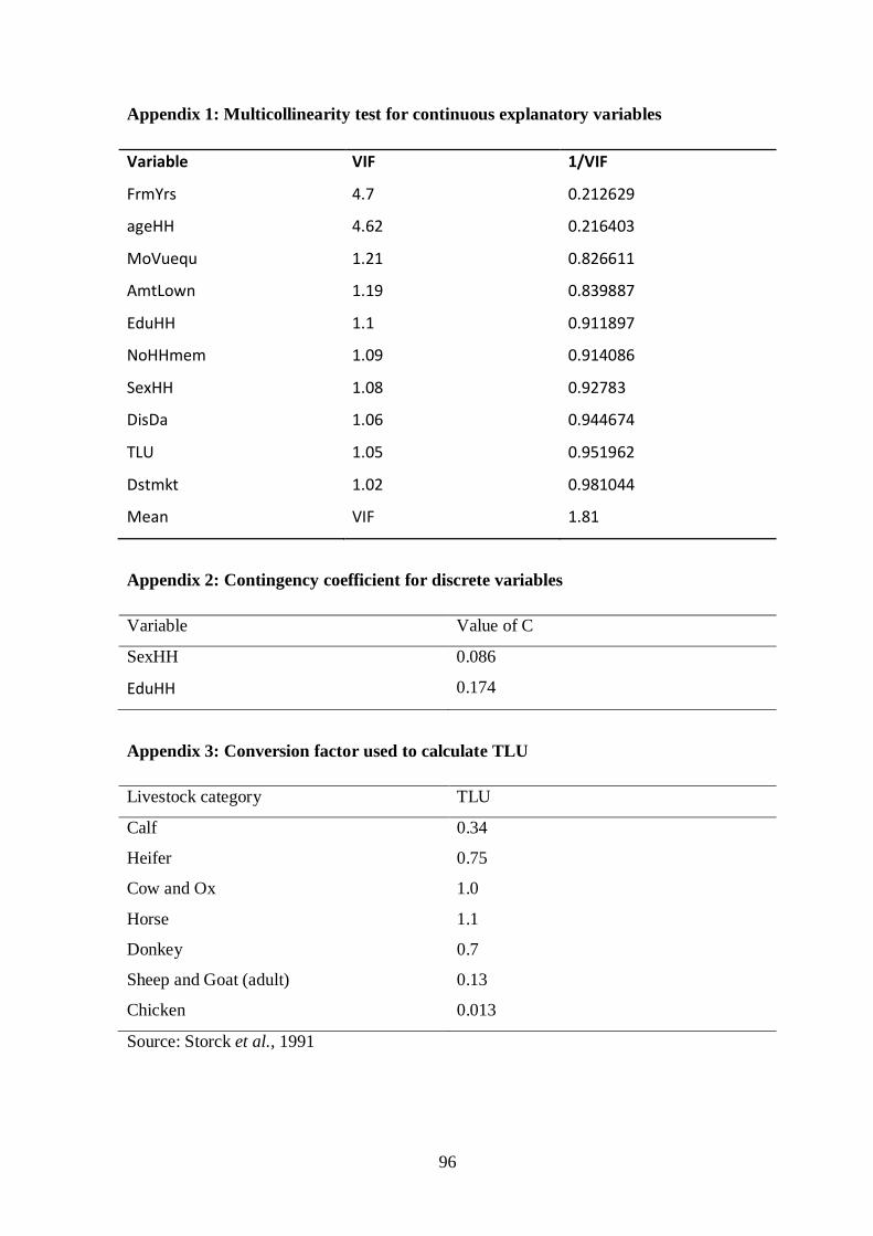
96
Appendix 1: Multicollinearity test for continuous explanatory variables
Variable VIF 1/VIF
FrmYrs 4.7 0.212629
ageHH 4.62 0.216403
MoVuequ 1.21 0.826611
AmtLown 1.19 0.839887
EduHH 1.1 0.911897
NoHHmem 1.09 0.914086
SexHH 1.08 0.92783
DisDa 1.06 0.944674
TLU 1.05 0.951962
Dstmkt 1.02 0.981044
Mean VIF 1.81
Appendix 2: Contingency coefficient for discrete variables
Variable Value of C
SexHH 0.086
EduHH 0.174
Appendix 3: Conversion factor used to calculate TLU
Livestock category TLU
Calf 0.34
Heifer 0.75
Cow and Ox 1.0
Horse 1.1
Donkey 0.7
Sheep and Goat (adult) 0.13
Chicken 0.013
Source: Storck et al., 1991

97
Appendix 4: Conversion factor for adult equivalent (AE)
Age group Male Female
<7 0.00 0.00
7-14 0.04 0.40
15-64 1.00 1.00
>65 0.50 0.50
Source: Storck, et al., 1991
Appendix 5: Histogram of Pscore with common (off) support regions
0 .2 .4 .6 .8 1Propensity Score
Untreated: Off support Untreated: On support
Treated: On support Treated: Off support

98
School of Graduate Studies
Department of Agricultural Economics
The Impact of Input and Output Market Development Interventions of the IPMS
Project: The Case of Meiso Woreda, Oromiya, Ethiopia
Questionnaire for individual household
Rigion: Oromia
Zone:
District:
Date of interview__________________________________________________________
Name of Peasant Association________________________________________________
Name of interviewee_______________________________________________________
Questionnaire no.__________________________________________________________
I. HOUSEHOLD CHARACTERSTICS
1.1. Name of household head,
1.2. Marital Status?
Married=1 Single=2 Divorced=3 Widowed=4
1.3. Sex of respondent?
Female=0 Male=1
1.4. Age of respondent? ___ (years)
1.5. Educational status? _____ (years) “1” if literate and ―0” if illiterate
1.6. Religion of respondent?
Orthodox=1 Muslim=2 Protestant=3 others (specify) ______________
1.7. Family size in age and sex groups
Table 1
S/N Name of household member Sex
1-male
2-female
Age R/ship to
head(a)
Education
level(b)
Major
occupation (c)

99
Codes a: Husband=1Wife=2 Son=3 Daughter=4 Other (specify)=5_____________
Codes b: No formal education=1 Adult education=2 Primary education=3
Secondary education=4 High school=5 Preparatory education=6
Certificate=7 Diploma=8 Degree=9
Codes c: Farming=1 Livestock raring=2 Herding=3 Household work=4
Marketing=5 Sell of fuel wood and charcoal=6 Petty trading=7
Schooling=8 Unemployed=9 Others=10 __________________________
1.8. Do you know the interventions of the IPMS project?
Yes =1 No =0
1.9. Did you participate in IPMS market development interventions?
Yes =1 No =0
1.10. If yes, for how long have you been beneficiary of the project? ____________ (years)
1.11. In which commodity of intervention did you participate?
1= Onion 2= Goat fattening 3= Cattle fattening
1.12. Total cultivated land in hectares
Owned land ______ Rented in land _________ Rented out land __________
Shared in_________ Shared out__________ Total land size possessed ________
1.13. Rate of land rental__________ Birr/ ha
1.14. What type of house do you have?
1=Corrugated iron sheet 2=Grass roofed 3=Kulu tora 4=Mud house
II. LIVESTOCK PRODUCTION
2.1. Livestock holding
Table 2
Livestock
types
Ox
Bull Barren
cow
Milking
cow
Heifers Sheep Goat poultry Donkey Camel
Number (in
head)
2.2.What are the main sources of feed in your area?
Grazing =1 hay =2 crop straw =3 others =4
2.3.Do you produce/plant improved forage for your livestock?
Yes=1 No=0

100
2.4. If yes, what is the size of land allotted for forage last years?
3. Table 3
Type of forage Mode of production
1= rain fed
2= irrigated
Size of land allotted Remark
Alfafa
Elephant plant
2.5. Do you sale improved forage?
Yes=1 No=0
2.6. Did the IPMS intervention improved feed availability?
Yes=1 No=0
2.7. If yes, how? _________________________________________________
2.8. What other benefit do you get from IPMS interventions related to feed?
______________________________________________________________
2.9. Have you brought change in the number of goat and cattle kept due to IPMS
intervention?
Yes=1 No=0
2.10. If yes, production in livestock and amount/number sold & income for the years of
intervention
Table 4
Livestock types Years of intervention
2008 2009
No. of
heads
Amt
sold
Price/head income No. of
heads
Amt
sold
Price/head income
Goat
Cattle
2.11. Specify IPMS support in Livestock production in your area
______________________________________________________________________
2.12. Have you participated in any of the local level livestock fair events in the past years?
Yes=1 No=0
2.13. If yes, what have you gained from participating in these fair events?
____________________________________________________________

101
2.14. Is there any change in productivity of livestock due to intervention by IPMS?
Yes=1 No =0
2.15. Did you have any goats and cattle meant for fattening in 2000/1?
Yes=1 No=0
2.16. If yes, what was your source, the type and cost of the livestock you have?
Table 5
Types of
livestock
Source of animal
1= own flock
2=purchase
Quantity Unit cost or
market value
(birr/head)
Remark
Goat
Cattle
2.17. Which types of shoat are more fattened?
Ram=1 Ewe=2 Keb (goromiti)=3 Wetete (Korbeessa)=4
2.18. How long it takes to finish fattening?
Goat ___________________
Cattle __________________
2.19. Have you purchased any inputs for livestock fattening purpose 2000/1?
Yes=1 No=0
2.20. If yes, would you tell us the following information?
Table 6
Type of inputs Does market
exist 1=Yes
2=No
Quantity Unit cost Total cost Source 1=traders
2=other farmers
3=OoPDR
4=cooperatives
Improved cow and
bull
Semen(lt.)
Vet. Service
Goat and cattle
forage
Forage seed
Nougcake (kg)
MUB (kg)
Hired labor
2.21. How often do you take fattened animals to market? __________________________

102
2.22. Is there any difference in the quality of animals after you started working with
IPMS?
Yes=1 No=0
2.23. If yes, how do you express the difference?
Poor=1 Good=2 Very good=3 Excellent=4
III. ONION PRODUCTION
3.1.Do you produce onion?
Yes=1 No=0
3.2. When did you start producing onion for your own? ____________________ (Years)
3.3. Have you ever participated in any intervention provided by IPMS in relation to onion?
Yes=1 No=0
3.4. Have you brought about change in land allocated to the commodities of intervention
due to IPMS intervention?
Yes=1 No=0
3.5. If yes, land allocation for commodity of intervention on the farm (ha)
Table 7
Commodity type Started to
participate since
(year)
Area allocated (ha) Remark
2008 2009
Onion
3.6. Out of the total land you have, how much did you allocate to the commodity that
IPMS has tried to develop through the value chain approach? ___________________
3.7. Specify IPMS support in onion production in your area ________________________
3.8. Production, amount sold & income for the years of intervention
Table 8
Commodity
type
Years of intervention Remark
2008 2009
Prod(qt) Amt.
sold
Price/qt income Prod(qt) Amt.
sold
Price/qt income
Onion

103
3.9. Have you sold any onion seed and seedling?
Yes=1 No=0
Table 9
Commodity
type
Years of intervention Remark
2008 2009
Prod(qt) Amt.
sold
Price/qt income Prod(qt) Amt.
sold
Price/qt income
Seed
Seedling
3.9. Is there any change in productivity of commodities of intervention of IPMS?
Yes=1No =0
3.10. If your answer is decreased what do you think is the reason? ___________________
3.11. If your answer is no change what do you think is the reason? __________________
3.12. How do you take production decisions?
1= traditional way 2= based on market signals 3= others (specify) __________
3.13. If you take decisions based on market signal, what is your source of information?
1= MOA, 2= IPMS, 3= others (specify) ____________________________
3.14. What do you think is the advantage of using market signal to take production
decision?
3.15. What problem did you face when you have been using market signal to make
production decisions? ___________________________________________________
A. LABOR
1. Provide information on utilization of labor in days spent per year for onion
production
Table 10
Commod
ity type
Source of labor
1=family 2=hired
3=labor
exchange, guza
Area
(ha)
Land
preparation
to planting
Weed
.
Harv Tran
s.
Storin
g
Marketin
g
Wage rate if hired
(birr/person/day)
Onion
2. Provide information on utilization of labor for goat and cattle production

104
Table 11
Commodity type Activities Source of labor
1=family2=hired
3=labor exchange,
guza
Days spent
per year
Current wage rate if
hired(birr/person/day)
Goat Housing
Feeding
Watering
Follow up and
monitoring
Medication
Marketing
Cattle Housing
Feeding
Watering
Follow up and
monitoring
Medication
Marketing
4. What is average working hours per day in onion production related activities? ___hours
B. USE OF OXEN
1. For which activities did you use oxen?
Plowing =1 Others (specify) ____________
2. Sources of oxen for plowing?
Own =1 hired/rented = 2 Borrowed = 3 others (specify) ____________
3. How much is the cost (rent) of pair of oxen in your area for plowing per day?
a) In cash____________________ Birr b) in kind _____________________
4. Provide information, if oxen were used for onion production
Table 12
Commodity type Area Oxen-pair days for
plowing
Remark
Onion
C. PESTICIDE
1. Did you use pesticide for onion production?
Yes =1 No =0

105
2. If yes, provide the following information on the use of pesticide
Table 13
Commodity
type
Area pesticide(kg) Unit cost Total cost Source 1=traders
2=other farmers
3= OoPRD
4=cooperatives
Onion
D. FERTILIZER USE
1. Do you use fertilizer in your onion fields?
Yes =1 No =0
2. If yes, when did you first use fertilizer on your farm? ________ (year)
3. If yes, type and quantity of fertilizer applied
Table 14
Commodity
type
Years of intervention
2008 2009
Area
(ha)
Quantity(kg) Cost/kg Area
(ha)
Quantity(kg) Cost/kg
Urea DAP Urea DAP
Onion
4. What is the reason for the above rate of fertilizer?
Own experience =1 Recommended =2 Others =3(Specify)________________________
5. If recommended, what was your source of information?
Extension=1 Research=2 NGOs=3 Other farmers=4 Others=5(specify) _______________
6. Is the current recommended fertilizer application profitable for you?
Yes =1 No =0
7. If no, which application rates do you suggest? _________________________Kg/ha
8. How was your fertilizer utilization changed due to IPMS?
Increased =1 Reduced =2 maintained the same =3 stopped using =4
9. If increased, why? ___________________________________________________
10. If reduced, why? ___________________________________________________
11. What constraints do you face on fertilizer use?
Inadequate supply =1 High price =2 Absence of fertilizer Credit =3 Bad weather =4 Not
profitable =5 Late delivery =6 Inappropriate loan repayment time =7 others =8(specify)

106
E. IMPROVED SEED
1. What is your source of improved seed for onion?
1=MOA 2=Cooperatives 3=Local market 4=other (specify) _________________
2. What is the improved seed rate used for commodities of intervention by IMPS
Table 15
Commodity type Years of intervention
2008 2009
Seed used
(kg/ha)
Price/kg Seed used
(kg/ha)
Price/kg
Onion
3. Did your use of seed improved change due to IPMS? Yes =1 No =0
4. INSTITUTIONAL FACTORS
A. Credit Service 4.1. Have you received any type of credit last year?
Yes=1 No=0
4.2. What is your source of credit?
1=Banks 2=Cooperatives 3=Microfinance institutions 4=OCSSCO integrated with IPMS
5= Other (Specify) _____________________
4.3. How much was it? _______________what was the interest rate? _________________
4.4. For what purpose you obtained the credit?
1. Seed purchase 2. Fertilizer purchase 3. Chemical/drug purchase
4. Animals purchase 5.To fill family requirement 6. To settle debt
7. For petty trade 8. Others (specify) _________________________
4.5. What are the problems/reasons in getting credit?
No need for credit=1 No credit available or few supply =2 Inadequacy of credit =3
Absence of informal sources =3 Unfavorable repayment time=4 High interest rates =5
Lack of collateral =6 others =7(specify) ________________
4.6. How do you rate the availability and adequacy of credit?
1=bad 2= moderate 3=good
4.7. Did IPMS done any contribution in relation to credit?
Yes=1 No=0
4.8. If yes, what, how, specify? _______________________________________________

107
B. Agricultural extension services
4.9. Did you participate in any extension program?
Yes=1 No=0
4.10. If yes, on which types of extension service you have been participated?
Demonstration=1 Training=2 Exhibition=3 Field day=4 5.
Others______________________
4.11. Have you attended farmer‘s training within last years?
Yes=1 No=0
4.12. If yes, how many days of training? _______________________________________
4.13. If you have participated on training would you tell us the content of the training?
1=Crop production 2=Animals production 3=Marketing strategy
4=Disease control 5=Natural resource conservation
6=Others (specify) _____________________________
4.14. Is there Agricultural Development Agent in your area?
Yes=1 No=0
4.15. If yes, do you get services or technical advice from development agents?
Yes=1 No=0
4.16. If yes, frequency of contact? ____________________ (total number of visits per
year)
4.17. What is the distance in Km from your home to the development agent's office or
residence? ____________________________________________________________
4.18. How many hours it requires you to walk from your home to the development agent's
office or residence? ____________________________________________________
4.19. What do you think is the contribution of IPMS for the extension service?
_______________________________________________________________________
4.20. Are you a member of any formal organization/association other than PAs?
Yes =1 No =0
4.21. If yes, which one?
Cooperatives =1 Women's group =2 Farmers‘ group=3 Others =4(specify) ____________
4.22. What services do you get from the formal organization you belong to?
Loans/credit =1 Seeds =2 Fertilizer =3 Labor =4 Education/information=5
Other=6 (specify) __________________________________
4.23. Have you ever made contractual agreement so far?

108
Yes=1 No=0
4.24. If yes, how do you rate the contractual agreements (keeping promises among
partners)?
1=low 2=moderate 3=high
4.25. Did IPMS made intervention on Cooperatives?
Yes=1 No=0
4.26. If yes, is there any change on cooperatives after IPMS intervention?
Yes=1 No=0
4.27. If yes, how?_______________________________________________________
V. FARM INCOME AND MARKETING
5.1. Where are your major markets for sale of farm products? _______________________
5.2. Distance of the nearest market in kilometers? __________ (walking hours ________)
5.3. Distance of the farthest market in kilometers? _________ (walking hours ________)
5.4. When do you sale most of your products?
1=Right after harvest 2=Later after harvest 3=Others ____________________________
5.5. What is your opinion on the prices of commodities in 2008/09?
Good = 1 Fair =2 Bad =3
5.6. Have you participated in off-farm activities in last year?
Yes=1 No=0
5.7. If yes, on what type of off-farm activities in last year?
Table 16
Types of off-farm
activities
Mode of participation
1= part-time(sometimes)
2= full time(throughout the
year)
Estimated
income
earned
Remark
Livestock trading
Crop trading
Firewood/charcoal
trading
Pottery making
Weaving
Leather making
5.8. How is the trend of your agricultural (on-farm) income since IPMS‘s intervention in
the PA?
Increased=1 Decreased=2 Remained unchanged=3
109
5.9. What was your total annual income from A) Crop sale _____birr B) Livestock sale
____birr? C) Sale of livestock products ____birr D) off-farm activity _____birr E) Others
(specify) ____ birr
5.10. What was your total annual expenditure for the last year?
A) Labor ____birr B) Purchase of farm tools ___birr C) Purchase of fertilizer ___birr D)
Purchase of seed ___birr E) Others (specify) _______birr
5.11. What are your sources of finance for purchase of agricultural inputs?
1=Crop sales 2=livestock sales 3=Off-farm activities 4=Credit
5=Others___________
5.12. Is there any change in market access?
Yes=1 No=0
5.13. If yes, how? _________________________________________________________
5.14. Do you get market information about prices and demand conditions of agricultural
outputs?
Yes=1 No=0
5.15. If yes, indicate the source of information
1=Radio 2=Merchant/traders 3= Development agents 4= Friends/ relatives/neighbors
5=Others (specify) ________________________
5.16. Do you get market information about prices and demand conditions of agricultural
inputs?
Yes=1 No=0
5.17. If yes, indicate the source of information
1=Radio 2=Merchant/traders 3= Development agents 4= Friends/ relatives/neighbors
5= Others (specify) ________________________
5.18. Do you feel IPMS brought benefit to you in providing market information using bill
board and speaker?
Yes=1 No=0
5.19. If yes, in what aspect? _________________________________________________
5.20. After IPMS information provision did you get better return/ price?
Yes=1 No=0
5.21. Did IPMS market information help you in reducing transportation costs in relation to
output markets?
Yes=1 No=0
5.22. If yes, how? _________________________________________________________

110
5.23. Did IPMS market information help you in reducing transportation costs in relation to
input markets?
Yes=1 No=0
5.23. If yes, how? _________________________________________________________
5.24. Do you know the input supply shop?
Yes=1 No=0
5.25. What benefit do you get from that shop? ___________________________________
VI. Perception Related Questions (Only For Participants)
6.1. In your opinion, how do you rate positive impact of the project in creating and linking
to market?
Poor=1 Good=2 Very good=3 Excellent=4
6.2. What is/are the rules and regulations you made with private traders if you made any
linkage?
________________________________________________________________________
________________________________________________________________________
________________________________________________________________________
__________________
6.3. Have you seen any negative impact of the project?
________________________________________________________________________
________________________________________________________________________
________________________________________________________________________
__________________