The Impact of High-Resolution Sea Surface Temperatures …weather.msfc.nasa.gov/sport/journal/pdfs/2008_MWR_LaCasse_etal.pdf · The Impact of High-Resolution Sea Surface Temperatures

The Impact of High-Resolution Sea Surface Temperatures on the Simulated NocturnalFlorida Marine Boundary Layer

KATHERINE M. LACASSE

University of Alabama in Huntsville, Huntsville, Alabama

MICHAEL E. SPLITT AND STEVEN M. LAZARUS

Florida Institute of Technology, Melbourne, Florida

WILLIAM M. LAPENTA

NASA Marshall Space Flight Center, Huntsville, Alabama

(Manuscript received 6 February 2007, in final form 24 July 2007)

ABSTRACT

High- and low-resolution sea surface temperature (SST) analysis products are used to initialize theWeather Research and Forecasting (WRF) Model for May 2004 for short-term forecasts over Florida andsurrounding waters. Initial and boundary conditions for the simulations were provided by a combination ofobservations, large-scale model output, and analysis products. The impact of using a 1-km ModerateResolution Imaging Spectroradiometer (MODIS) SST composite on subsequent evolution of the marineatmospheric boundary layer (MABL) is assessed through simulation comparisons and limited validation.Model results are presented for individual simulations, as well as for aggregates of easterly- and westerly-dominated low-level flows. The simulation comparisons show that the use of MODIS SST compositesresults in enhanced convergence zones, earlier and more intense horizontal convective rolls, and an increasein precipitation as well as a change in precipitation location. Validation of 10-m winds with buoys shows aslight improvement in wind speed. The most significant results of this study are that 1) vertical wind stressdivergence and pressure gradient accelerations across the Florida Current region vary in importance as afunction of flow direction and stability and 2) the warmer Florida Current in the MODIS product transportsheat vertically and downwind of this heat source, modifying the thermal structure and the MABL wind fieldprimarily through pressure gradient adjustments.

1. Introduction

Predicting mesoscale phenomena affecting the spa-tial and temporal distribution of temperature, wind,and precipitation is a common forecast challenge alongthe Florida peninsula (e.g., Bauman and Businger1996). Large gradients in sea surface temperature(SST) east of central Florida associated with the FloridaCurrent (FC) during the late spring and summer have adirect impact on the development of offshore second-ary solenoids (Sublette and Young 1996), cumuluscloud lines (Li et al. 2004), and stratocumulus cloud

fields. Figure 1 shows cloud features on 17 May 2004that typify some of the complex SST-influenced fea-tures of the summer season. Features of note include alow-level cumulus field over the FC, north of theBahamas, horizontal convective rolls associated withand downwind of the Bahamas, and convection overthe Florida–Hatteras shelf (FHS) along the westernedge of the FC. Figure 1 also depicts a lack of cumu-lus over the cooler FHS waters and a relatively clearregion west of the Florida peninsula as easterly low-level flow moves from the warmer peninsula to thecooler SSTs.

Numerous studies using satellite-derived and conven-tional observations have shown a positive correlationbetween SST fields and near-surface wind stress atscales of 1000 km or less (e.g., Chelton et al. 2001;O’Neill et al. 2003; Tokinaga et al. 2005). Modeling

Corresponding author address: Katherine M. LaCasse, Univer-sity of Alabama in Huntsville, 320 Sparkman Dr., Huntsville, AL35805.E-mail: [email protected]

APRIL 2008 L A C A S S E E T A L . 1349

DOI: 10.1175/2007MWR2167.1

© 2008 American Meteorological Society

MWR2167

studies have also simulated this relationship. Small etal. (2003) explored the importance of three processesinvolved in the response of the marine atmosphericboundary layer (MABL) to tropical instability wavesusing a regional climate model. For that case, verticalmixing was important to latent and sensible heat fluxesand horizontal mixing had a small effect by advectingthe SST impact downstream. The horizontal perturba-tion pressure gradient was shown to be significant, be-cause it drove the near-surface wind speed changesacross the SST gradients. In a study by Song et al.(2004), the fifth-generation Pennsylvania State Univer-

sity–National Center for Atmospheric Research Meso-scale Model (MM5) was used to study the impact of aSST front on the MABL at high resolution (3-km gridresolution). Two separate cases were evaluated, and thesimulated MABL response to the imposed SST fieldscompared well to the observations collected via air-craft. This result lends confidence to the claim that theuse of high-resolution SSTs in a mesoscale model canproduce a realistic simulation of the MABL. Chelton(2005) investigated the impact of SST spatial resolutionusing the European Centre for Medium-RangeWeather Forecast (ECMWF) system. Forecasts were

FIG. 1. MODIS visible composite valid at 1855 UTC 17 May 2004. Cloud features of note include a low-level cumulus field over theFlorida Current, horizontal convective rolls associated with and downwind of the Bahamas, convection over the Florida–Hatteras shelfalong the western edge of the Florida Current, and a lack of cumulus over the cooler Florida–Hatteras shelf waters and west of theFlorida peninsula.

1350 M O N T H L Y W E A T H E R R E V I E W VOLUME 136

Fig 1 live 4/C

conducted and compared using the 1° Reynolds SSTfield and the 0.5° real-time global (RTG) SST analyses.Use of higher-resolution SST data resulted in forecaststhat compared more favorably with near-surface windstress as derived from the National Aeronautics andSpace Administration (NASA) Quick Scatterometer(QuikSCAT) instrument on board the Tropical Rain-fall Measuring Mission (TRMM) Microwave Imager(TMI). Initialization of a mesoscale model with calmwind and flat horizontal pressure gradients showed adirect correlation between the strength of the SST gra-dient and simulated thermal and moisture gradientswithin the MABL associated with an atmospheric frontin the vicinity of the Gulf Stream (Warner et al. 1990).Despite the various boundary layer formulations used,each of these studies indicates sensitivity to the under-lying specification of the SST.

As the horizontal resolution of operational numericalweather prediction models continues to increase, it hasbecome increasingly important to properly specify thespatial heterogeneity associated with land surface forc-ing (i.e., soil moisture, vegetation characteristics, etc.).While the diurnal signal of SST is typically much lessthan that over land, in calm conditions it can be signif-icant (Minnett 2003). Moreover, resolving SST fea-tures, especially mesoscale gradients in the near-shoreenvironment, is inarguably an essential component withrespect to the improvement of coastal zone forecasts ofboundary layer clouds and precipitation, accuratespecification of surface fluxes, etc. Current operationalforecast Models [e.g., the North American Mesoscale(NAM) model and the ECMWF model] are initializedwith a 0.5° SST analysis produced daily at the NationalCenters for Environmental Prediction (NCEP;Thiébaux et al. 2003). The purpose of this study is toexamine the impact of using high-resolution (1 km) SSTfields derived from the NASA Earth Observing SystemModerate Resolution Imaging Spectroradiometer(MODIS) on the overlying MABL thermodynamic andkinematic structures as simulated by the Weather Re-search and Forecasting (WRF; Skamarock et al. 2005)modeling system run at 2-km resolution over theFlorida peninsula.

The paper is structured as follows. Sea surface tem-perature products are described in section 2. Section 3contains a description of the WRF configuration andexperiment design. Results are presented in section 4,followed by the summary, conclusions, and suggestionsfor future work in section 5.

2. Sea surface temperature products

The purpose of this study is to examine and under-stand how the spatial resolution of SST fields used

within a state-of-the-art numerical weather predictionsystem affects simulations of MABL evolution andstructure. Therefore, two SST products are employed.The first is the operational NCEP RTG product that isused in the NCEP operational NAM and Global Fore-cast System modeling suite. The RTG is the default SSTfield used by the majority of the WRF user community.The second is a prototype SST product derived fromMODIS that is not yet available to the WRF commu-nity.

a. Real-time global sea surface temperature analysis

The RTG SST analysis is produced daily by theNCEP Marine Modeling and Analysis Branch. Theanalysis is created using a two-dimensional variationaldata assimilation scheme, with the previous analysis,adjusted for climatology, providing the backgroundfield (Thiébaux et al. 2003). Observations from the past24 h, as well as previously unused in situ observationsup to 36 h old, are averaged within each grid box foreach observation type. The observations include shipand buoy data as well as satellite-derived SST from theNational Oceanic and Atmospheric AdministrationAdvanced Very High Resolution Radiometer. A spa-tially varying Gaussian error decorrelation length scaleis defined to be inversely proportional to the climato-logical SST gradients (Thiébaux et al. 2003). This en-sures that the SST observations are given a smaller(larger) radius of influence in regions of strong (weak)SST gradients. Global analyses are created operation-ally once daily at both 0.5° and 0.083° spatial resolution.Only the 0.5° product was available during the casestudy period of May 2004 and is used for the WRFRTG simulations herein. The RMS errors for this prod-uct, in comparison with those of buoys, range between0.4°–0.6°C for 30°S–30°N and 0.6°–1.2°C for 30°–90°N(Thiébaux et al. 2003). The 0.5° grid also provides theSSTs for numerous operational models, including theNAM, the rapid update cycle (RUC), and the ECMWFmodels.

b. MODIS sea surface temperature composite

The MODIS instrument, on both the NASA Aquaand Terra polar-orbiting satellites, uses clear-sky infra-red channels to retrieve SST. In particular, brightnesstemperature from both the 11- and 12-�m channels, aswell as a climatological estimate of SST, contributes tothe MODIS SST value. These SST products have beencompared with buoys and have errors of 0.5°C (Minnettet al. 2007).

The 1-km MODIS SST composite used in this work isa prototype dataset currently produced at the NASA


Short-Term Prediction Research and Transition(SPoRT) Center. It is produced by combining multiplepasses of the 1-km Earth Observing System MODISSST data in order to reduce spatial gaps caused by passlocation and/or cloud contamination. The compositingapproach is based on the assumption that the day-to-day variation of SST is relatively small. The validity ofthis assumption may vary spatially and seasonally asoceanic and atmospheric forcing creates higher-frequency changes in SST values (e.g., cooling in thewake of a hurricane). Data from both MODIS plat-forms are combined to create separate day/night com-posites using the five most recent clear-sky SST valuesfor each pixel. Daytime (nighttime) Aqua and Terrapasses through the composite region occur at approxi-mately 1330 and 1030 (approximately 0130 and 2230)LT, respectively. Four distinct composites are createddaily by combining data that correspond to the sametime of day in order to capture as much of the diurnalsignal as possible. The composite method used for thisstudy averages the warmest three of the five pixels inorder to mitigate the impact of cloud contamination.For the month of May 2004, the warmest pixels are alsothe most recent.

The MODIS SST composites used in this study havebeen verified against buoys and appear to represent theSST field well with RMS errors less than 0.7°C (Haineset al. 2007). A comparison of the MODIS compositewith a clear MODIS pass reveals that the compositeretains the strength of the SST gradients (not shown).Alternative compositing methodologies are currentlyunder development in an attempt to decrease productlatency, while capturing short-term changes in the SSTs(S. L. Haines 2006, personal communication).

c. A comparison of RTG and MODIS SSTproducts

A representative day (13 May 2004) from the studyperiod is chosen to highlight the differences betweenthe MODIS SST composites and RTG SST analyses.Figure 2 shows both fields after being mapped onto the2-km WRF grid used for this study. The large-scalestructures observed in the SST fields are similar, asexpected, with values varying by only 1°C. However,the MODIS SST composite clearly has more finescaledetail than the RTG SST analysis, both offshore andalong the immediate coast. The Florida Current andGulf Stream are discontinuous off the northern Floridacoast and are poorly resolved in the RTG. In addition,the RTG SST analysis underestimates the southern ex-tent of the near-shore cool wedge off the east coast ofFlorida, resulting in temperatures 0.5°–2°C warmerthan the MODIS SST composite.

Differences between the analyses described abovepersist throughout May 2004 and have a relatively sig-nificant impact on the magnitude and location of theSST gradient along the western edge of the FloridaCurrent. Figure 3 shows a plot of the two SST analysesacross the western boundary of the Florida Current, aswell as the heat content within the Florida Current. TheMODIS SST composite exhibits a gradient of approxi-mately 2°C in a 40-km distance, while the SST in theRTG analysis is virtually flat and exhibits no gradient atall. The absence of such mesoscale SST features will beshown to have an impact on the simulation of theMABL and associated sensible weather elements incoastal regions.

3. Model description and experiment design

A coupled atmospheric data assimilation and fore-cast system was employed to examine the impact ofhigh-resolution SST fields on simulated MABL struc-tures using real data cases. A description of the dataassimilation, model configuration, and a detailed de-scription of the experiment design follows.

a. ARPS Data Analysis System

The Advanced Regional Prediction System (ARPS;Xue et al. 2000) consists of several components, includ-ing a data assimilation system [ARPS Data AnalysisSystem (ADAS)]. The ADAS is used to generate initialconditions for the WRF model used in this study. It isan iterative successive correction scheme, commonlyreferred to as the Bratseth method, which converges tooptimal interpolation (Bratseth 1986). This scheme isconvenient because it is computationally less demand-ing than other data assimilation methods (such as varia-tional techniques). The number of iterations, type ofdata, and order of assimilation are user controlled,which preferentially allows the large-scale observationsto adjust the background field, followed by the smaller-scale data. The error variances assigned to the obser-vations and the background field, as well as the dis-tances between observations and grid points, determinehow much influence the observations will have on theanalysis. Horizontal and vertical scaling distances arealso specified for each iteration, and errors are speci-fied for each type of observation. The assimilationmethod is further described in Brewster (1996) andLazarus et al. (2002).

Observations assimilated in this study include theAviation Routine Weather Reports (METARs), buoys,Aircraft Communication Addressing and ReportingSystem (ACARS), rawinsondes, wind profilers, and


FIG. 2. SSTs (K) mapped to the WRF domain (2-km resolution) valid 13 May 2004 for (a)RTG SST analysis and (b) daytime Aqua MODIS SST composite. The solid black line east ofCape Canaveral in (b) indicates the cross section depicted in Fig. 3. Dotted lines represent thesignificant ocean currents within the domain.


Fig 2 live 4/C

Florida Weather Surveillance Radar-1988 Doppler(WSR-88D) level II radar radial winds. Estimates ofobservation errors for these commonly used data typesare provided with the ARPS code, and for this study,the default values are used. The observations are ana-lyzed on the three-dimensional ADAS grid for the uand � component of the wind, pressure, potential tem-perature, and specific humidity. Quality control mea-sures include a buddy check with nearby observationsand a comparison with the background field. Surfacedata are also checked against observations from a priortime, in this case the previous hour. The WSR-88Dlevel II radar data are remapped for the ARPS grid byaveraging the data within each 3D grid box and refor-matting the data for the ADAS (Brewster 1996).

The proper specification of land surface conditionsfor this study is an important component of the experi-ment design because the diurnal variation of the plan-etary boundary layer (PBL) over land is known to be astrong forcing factor in the development and evolutionof mesoscale atmospheric phenomena in the Floridacoastal regions. The best possible representation of soilmoisture conditions for the study period was obtainedusing antecedent precipitation and near-surface meteo-rological data over a 4-month period in an offline modeto force the soil model. To obtain the best possibledefinition of the coastline, the 3-s U.S. Geological Sur-vey data were used.

b. The WRF prediction system

The WRF prediction system consists of two dynami-cal cores—the Advanced Research WRF (version 2.1.0is used herein) and the Nonhydrostatic MesoscaleModel. The WRF model is modular, allowing users to

easily select different combinations of physics schemes,and it is optimized for parallel computing environ-ments. The physics options used in this study includethe Noah land surface model, the Yonsei University(YSU) PBL scheme, WRF single-moment six-class(WSM-6) microphysics, Dudhia shortwave radiation,and Rapid Radiative Transfer Model (RRTM) long-wave radiation. To properly gauge the impact of theSSTs, the components involving surface–atmosphereinteraction are of particular importance. The four-layersoil temperature and moisture model, Noah (Chen andDudhia 2001), provides heat and moisture fluxes for theYSU PBL scheme (Hong et al. 2006). The YSU PBLscheme uses nonlocal K mixing and treats entrainmentat the top of the PBL explicitly. The YSU PBL schemewas chosen after comparisons against the Mellor–Yamada–Janjic (Mellor and Yamada 1982; Janjic 1994)turbulent kinetic energy (TKE) PBL scheme revealedrelatively small differences in the control forecasts andcomparable impact due to the MODIS SSTs (notshown). However, in some instances, the scheme-to-scheme (PBL) variability is on the order of that of theimpact of the SSTs on the simulations. This choice isconsistent with recently published work of Song et al.(2006), which indicates that MM5 simulations using theMRF PBL scheme (i.e., the YSU predecessor) yieldedthe best results of the five boundary layer models whencompared directly against observations.

c. Experiment design

WRF simulations were conducted over a region thatincludes Florida, the eastern Gulf of Mexico, and theAtlantic coastal waters of east Florida (Fig. 2). Thedomain consists of 500 � 500 horizontal grid points at2-km resolution with 51 vertical levels. The lowestsigma levels were spaced every 0.01 between 1.00 and0.90, which is a sufficient resolution for the calculationof surface fluxes (Hong et al. 2006). A series of 24-hsimulations conducted each day during May 2004 wereinitialized at 0000 UTC. The National Climate DataCenter (NCDC) ranked May 2004 as the fourth driestMay on record for the state of Florida for the period of1895–2004 (NCDC 2004). May 2004 was selected forthis study because it represented a relatively clear pe-riod when few synoptic-scale frontal systems propagat-ed south of 30°N, allowing the marine boundary layerto be strongly modulated by the underlying SST. Al-though a period with clouds and precipitation wouldalso be of interest, it was our desire to mitigate com-plications associated with convection. Because of thequiescent period chosen, the impact of the MODISSSTs will be primarily confined to the MABL. Addi-

FIG. 3. Value of RTG SST (solid) and MODIS SST (dashed) asdescribed in Fig. 2. Line is taken at 29.01°N latitude and 80.49°–80.10°W longitude, as drawn on Fig. 2b.


tional benefits of choosing a dry period include the fol-lowing: 1) fewer cloud-contaminated pixels, resulting inreduced composite latency, and 2) weak synoptic flow,which enables the configuration of a solitary, computa-tionally efficient model grid without the introduction ofspurious boundary condition problems resulting fromlarge-scale forcing.

Two sets of numerical experiments were performed.One model configuration (experiment), referred tohere as RTG, employed the 0.5° RTG SST product forlower boundary forcing over the ocean. The secondexperiment, referred to as MODIS, was identical theRTG in every way, except that the 1-km MODIS SSTcomposite was used in place of the RTG SST analysis.The experiment design, in part, was chosen so as toallow the atmospheric boundary layer to adjust to theunderlying sea surface prior to the forecast period. Anintermittent data assimilation (IDA) cycle was imple-mented over a 3-h window prior to the forecast. Albeitsomewhat short, the 3-h window is consistent with pre-vious mesoscale modeling studies (e.g., Xue and Martin2006; Dawson and Xue 2006). The IDA is launched at2100 UTC, using the RUC-20 as a first guess, and theassimilated observations are described in section 3a.Because the RTG analysis is used within the suite ofNCEP operational models (both the RUC-20 and EtaModel are initialized with the RTG), any adjustmentsin response to the lower boundary will manifest in theMODIS simulations only. Regardless, it is worth point-ing out that the upwind marine boundary layer is con-tinuously adjusting to SST variations. Lateral boundaryconditions (LBCs) for the 3-h WRF simulation endingat 0000 UTC were derived from RUC analyses. The 3-hWRF forecast was then used as the background fieldfor a second ADAS cycle at 0000 UTC to create theinitial conditions for the subsequent 24-h forecast. The0000 UTC ADAS analysis ensures that the initial con-ditions of the RTG and MODIS experiments are com-parable where observations exist. The LBCs for the24-h forecast period were obtained from the 40-kmNCEP Eta Model grids at 3-hourly intervals. TheMODIS composites used were obtained from the after-noon Aqua pass and were valid at approximately 1900UTC daily. The SST fields were static during the 3-hassimilation and 24-h forecast periods. With the excep-tion of the SSTs, both the RTG and MODIS runs areidentical. To avoid the negative impact of spurious con-vection, which can promote significant error growth inshort-term deterministic mesoscale forecasts (e.g.,Zhang et al. 2006), we intentionally avoid the continu-ous/sequential data assimilation approach (Lorenc1995) whereby the prior 24-h forecast is used to initial-ize the next cycle.

4. Results

One of the chief advantages of using the MODIShigh-resolution SST fields in numerical weather predic-tion is the representation of mesoscale structures.Therefore, emphasis is placed on examination of theMABL structures in regions where strong SST gradi-ents were found to exist, such as with the Florida Cur-rent and shelf waters (Fig. 2). Previous studies haveshown that the MABL responds to flow across SSTgradients (e.g., Song et al. 2004; O’Neill et al. 2005;Tokinaga et al. 2005).

Results from individual daily simulations will be pre-sented. However, the most relevant impacts of the SSTgradients were obtained by stratification of simulationsaccording to the direction of low-level flow across thegradient, as discussed above. May 2004 included 10easterly and 4 westerly flow cases, accounting for half ofall of the simulations for the month. This a priori se-lection of regimes grouped together simulations inwhich the surface winds have a large normal compo-nent to the SST gradient along the western boundary ofthe Florida Current. Low-level gradient parallel flowdid occur along portions of this SST gradient duringportions of the simulations, and, in previous studies, hasbeen shown to be beneficial to the enhancement of asolenoidal circulation between the cool and warm wa-ters (e.g., Li et al. 2004). To isolate the impacts associ-ated with the relatively quiescent nocturnal period,nighttime aggregates were composited by averaginghourly WRF output between 0500 and 1100 UTC. Ad-ditionally, a nine-point spatial smoother is applied tothe output to isolate the mesoscale signal from smaller-scale noise.

a. Overview of simulation differences

Prior to discussing the aggregate results, a summaryof some of the relevant differences between the modelsimulations is briefly presented here. Substantial differ-ences in sea-breeze strength and onset time were notobserved in the simulations, despite the fact thatMODIS SST has significantly more detail. However, thisis not surprising because the primary forcing mecha-nism for the sea-breeze circulation is associated withdiurnal heating of the land surface, which is essentiallyidentical for both the RTG and MODIS experiments.The MODIS simulations generated an earlier onset andgreater amount of turbulent structure such as horizon-tal convective rolls (HCRs) over the marine area. Dailyaccumulated precipitation over the full domain was en-hanced in the MODIS simulations by 5.9% over theentire month of May 2004. Subsections of the grid pro-duced more dramatic differences. In an area defined


from the Bahamas, west to the Florida Straits, the pre-cipitation increased by 11.7%, while in an area alongthe Florida Current precipitation increased by 27.3%for these MODIS cases.

Extended surface convergence zones, such as thatassociated with the Gulf Stream atmospheric frontnoted by Li et al. (2004), are observable in a few of themodel runs. Figure 4 illustrates an example in which the12-h MODIS simulation, valid at 1200 UTC 6 May2004, produces elongated convergence zones over boththe Florida Current and the transition zone betweenthe Florida Current and the Florida–Hatteras shelf. Al-though on this particular day only one of the conver-gence zones appears to be associated with a cumuluscloud line, these features are typical of those observedin this region and are often precursors to deep convec-tion, especially nocturnally (e.g., Lericos et al. 2002).The WRF simulations for 16 May 2004 develop convec-tion early in the forecast period along two differentboundaries. The RTG develops convection along theeast-central Florida coast where convergence occurs(Figs. 5a,c). In contrast, the MODIS simulation devel-ops convection to the east of this location along thesignificant SST gradient that is captured in the high-resolution SST product (Figs. 5b,d). Radar and visiblesatellite data (not shown) indicate that a line of con-vection developed west and downwind of the Bahamas,and streamed into the Florida peninsula just to thesouth of the noted convection in the WRF simulations.While neither model run captures this area of convec-tion successfully, the change in location of the modelprecipitation from along the coast to just offshore issignificant from an operational perspective. Addition-ally, the impact illustrates the sensitivity of the WRF tohigh-resolution SSTs. For this particular event, the SSTspecification appears to be a secondary issue as themesoscale forcing associated with the generation ofprecipitating cloud systems over and downwind of theBahamas dominates. Enhanced low-level convergenceand precipitation, formed along the SST gradient in theMODIS simulations, are commonly observed over thecoastal waters of this region and are visible as cloudlines in both radar and satellite images.

b. Easterly and westerly flow regimes

As previously discussed, aspects of the MODIS SSTimpact for specific wind regimes are more easily dis-cerned with composite statistics. Aggregate 10-m windfor both the easterly and westerly flow regimes areshown for the nocturnal period in Fig. 6. Differences inthe wind direction between the two regimes are mostsignificant over the northern portions of the domain,especially along the Florida Current. The focus is on

the waters off the eastern coast of Florida where east-erly (westerly) flow is associated with the transit of airparcels from (to) the warm Florida Current waters to(from) the cooler shelf waters. The following results arebased on the easterly and westerly regime specifica-tions.

1) SURFACE AND INTEGRATED FIELDS

(i) Surface fluxes

In a related study, Rouault et al. (2003) noted rela-tively significant errors in simulated latent and sensibleheat fluxes over the Agulhas Current, a western bound-

FIG. 4. Visible GOES image from 1130 UTC 6 May 2004 withWRF surface convergence (contours, every 0.5 s�1 � 106) at 1200UTC (12-h forecast) for (a) MODIS and (b) RTG. A line ofcongested cumulus in the northeast portion of the domain coin-cides with an elongated zone of convergence in the MODIS simu-lation, while a second convergence zone along the Florida–Hatteras shelf was not associated with low-level cloud develop-ment. The RTG does not produce significant convergence.


ary current near Africa that has sharp SST gradients.These errors were in part shown to be related to the useof low-resolution SST products. A comparison betweenthe two SST products used herein is shown in Fig. 7,depicting the average SST differences (MODIS �RTG) for the easterly and westerly flow regimes. Posi-tive differences in SST (where the MODIS SST com-posite is warmer) along the Florida Current, for ex-ample, indicate where the MODIS SST product bettercaptures the higher-resolution detail. The westerly flowregime shows negative differences, which are clearlymore confined to the near-coastal region than in theeasterly flow regime. This may be attributed to up-welling in the inner shelf. For brevity, the differences insurface sensible and latent heat fluxes are shown for the

nocturnal easterly flow cases only (Figs. 8 and 9, re-spectively). Positive (negative) differences in SST areassociated with increased (decreased) surface sensibleand latent heat fluxes. Sensible heat fluxes increased inthe MODIS runs by as much as 100% in the FloridaCurrent, while latent heat flux increases approached30%. These differences provide an initial indicationthat the WRF is sensitive to the high-resolution SSTs.

(ii) Mean sea level pressure

Differences in the sensible and latent heat fluxesshould impact the evolution of other state and kine-matic fields. For example, Tijm et al. (1999) have shownthat the pressure field responds to changes in the sur-face fluxes between land and ocean associated with the

FIG. 5. Model reflectivity (dBZ ) 3-h forecast valid at 0300 UTC 16 May 2004 for (a) RTG, (b) MODIS; model convergence, spatiallyfiltered and smoothed (shaded for values greater than 2 and 4 s�1 � 10�4) for (c) RTG and (d) MODIS. The RTG simulation producesthunderstorms along the coastal convergence zone, while the MODIS simulation generates convection along a convergence zone on thewestern edge of the Florida Current close to 80.0°W.


Fig 5 live 4/C

sea breeze. Here, the largest impact on the sea levelpressure (SLP) field is simulated to be downwind of thesignificant changes in the surface heat flux, especially inthe vicinity of the Florida Current and the Bahamas.The easterly flow regime shows two distinct regions inwhich the MODIS simulations produce lower SLP:over southeast Florida and off the Florida northeastcoast just west of 80.0°W (Fig. 10a). In contrast, for thewesterly flow cases, the two negative pressure anoma-

lies are shifted eastward (Fig. 10b). The different re-sponses in SLP between the two regimes illustrates theimportance of flow-dependent (i.e., advective) effectsthat act to displace the response downstream of theforcing. The use of the MODIS SST composite pro-duced changes in average sea level pressure of up to 8Pa, which are on the order of that observed with me-soscale phenomena, such as sea or lake breezes.

(iii) Kinematics

The impact on the surface wind field in response tothe pressure forcing (i.e., changes in the pressure gra-dient) has been documented in other studies (e.g.,Lindzen and Nigam 1987). The pressure gradient modelis analogous to the sea-breeze circulation, wherebychanges in SSTs lead to a change in surface fluxes anda subsequent thermal response in the MABL. Warmer(cooler) SSTs lead to lower (higher) sea level pressure,thereby modifying the pressure gradient and producingsurface wind accelerations (decelerations). In an alter-native model, changes in the MABL stability (and thusvertical wind stress divergence) across an SST gradientinduce surface wind accelerations (e.g., Wallace et al.1989; Koracin and Rogers 1990). The transit of air par-cels across SST gradients has been investigated in thiscontext (Song et al. 2004; Song et al. 2006; Nonaka andXie 2003). It has been shown to impact the flow differ-ently for parcel trajectories moving parallel to the tem-perature gradient (Samelson et al. 2006). In particular,Samelson et al. (2006) show that the wind and tempera-ture profiles reflect a well-mixed layer over warm SSTs.In this case, a warming of SSTs leads to a less stableMABL. This causes both an increase in mixing and ahigher surface stress (but decreased vertical wind stressdivergence), which is reflected by faster winds near thesurface. Additionally, past studies have shown thatmodels tend to underestimate the relationship betweenthe wind stress and SST, especially in regions of signifi-cant gradients (Maloney and Chelton 2006).

The two mechanisms discussed previously are re-ferred to here as follows: 1) vertical wind stress diver-gence (parcel wind speed changes associated with sta-bility changes within the surface layer and/or a shallowinternal boundary layer; e.g., advection of warm airover cooler waters) and 2) pressure gradient forcing(parcel accelerations resulting from the modification ofthe pressure gradient). The comparison of the MODISand RTG runs pressure fields will be referred to asperturbation pressure gradient forcing. For the easterlyflow regime, surface air parcels pass over the warmFlorida Current to the cooler shelf waters with the ex-pectation that parcel deceleration may be caused byeither forcing mechanism—(a) an increased vertical

FIG. 6. Nocturnal mean 10-m wind speed and direction (m s�1)for (a) easterly and (b) westerly wind regimes during May 2004.The solid black lines in (a) and (b) represent the axes of the crosssections shown in Fig. 19.


FIG. 7. May 2004 mean SST differences (MODIS � RTG; K) for (a) easterly and (b) westerly flowregimes. Black squares on (b) indicate locations of buoys used for model verification.


Fig 7 live 4/C

wind stress divergence within the enhanced stability ofthe cooler shelf waters or (b) the eastward-pointed per-turbation pressure gradient in that region (Fig. 10a).Figure 11 depicts the impact of the MODIS SST com-posites on the simulated 10-m winds and shows decel-erating (accelerating) flow across the enhanced SST

gradient under easterly (westerly) flow regimes consis-tent with either forcing mechanism. While the pertur-bation pressure gradient forcing is consistent with themodeled deceleration for the easterly-flow case, itwould be expected to lead to a larger acceleration (andhence a more positive wind difference than that ob-served) east of the perturbation pressure gradient mini-mum (gray box in Fig. 11a). In fact, there is only weakacceleration in this region (Fig. 11a). To better under-stand the acceleration differences, the various forcing

FIG. 9. As in Fig. 8, but for surface latent heat flux difference(W m�2).

FIG. 8. Average difference in surface sensible heat flux (W m�2)between MODIS and RTG runs for nocturnal easterly-flow cases.

FIG. 10. As in Fig. 8, but for mean sea level pressure difference(Pa) for (a) easterly- and (b) westerly-flow regimes.


components (i.e., pressure gradient force, Coriolisforce, and vertical winds stress divergence) were calcu-lated (Fig. 12). The vertical wind stress divergence wascalculated as a residual acceleration because the WRFdoes not explicitly output this acceleration for the sur-face. For the easterly flow cases, the perturbation pres-sure gradient force acts to accelerate the wind, whilethe vertical wind stress divergence generally works to

decelerate the flow in this region (gray box, Fig. 12a).Conversely, for westerly flow, the vertical wind stressdivergence overwhelms the pressure forcing in the re-gion of significant positive wind differences (grayboxes, Figs. 11b and 12b). For these cases, very stablelow-level air is advecting off the Florida peninsula [seesection 4b(2)], thereby limiting the depth of the verticalresponse. Although the largest perturbation pressuregradient vectors are in the northeast portion of the do-main (Fig. 12b), these tend to oppose the stress diver-gence vector, thereby mitigating the impact on the winddifferences (note the smaller secondary positive winddifference to the northeast of the main signal in Fig.11b). Furthermore, these large perturbation pressuregradient vectors are an artifact of convection, whichoverwhelms the more subtle mesoscale signal respon-sible for the wind differences shown in Fig. 11 (notshown). The response to the high-resolution SSTs isflow dependent, with about twice as much response inthe wind speed along parcel trajectories that transitionfrom cool to warm. Wind speed changes betweenMODIS and RTG runs are on the order of 6% (9%) inthe westerly (easterly) flow regime in the vicinity of theFlorida Current (not shown). Qualitatively, the impactof the high-resolution SST product in the WRF modelproduced changes in the wind field that are consistentwith recent studies.

While the impact on the wind field is relevant, it isalso instructive to evaluate changes in surface diver-gence because wind speed accelerations previouslynoted might be largely compensated for by directionalchanges to the wind. The response of this derived fieldfor May 2004 is also flow dependent, with an increase inconvergence to the west of the significant SST gradient(associated with the west side of the Florida Current)for the nocturnal easterly flow cases (Fig. 13a). A con-vergence zone associated with the western edge of theGulf Stream has been noted by Raman et al. (1998) tobe associated with a coastal front; however, that caseconsisted of a significant synoptic-scale temperaturegradient and trough. Here, convergence axes shifted tothe east of the SST gradient for westerly flow cases (Fig.13b), with the changes in convergence being a factor of2 larger in magnitude and spatially more coherent thanin the easterly flow cases. The accelerations in the sur-face winds introduced by the use of the MODIS SSTproduce changes to the surface divergence that aremore pronounced in the SST gradient regions.

(iv) Boundary layer height

Changes in the depth of the mixed layer are antici-pated as a result of the differences in the surface heatfluxes in the simulations. The WRF boundary layer

FIG. 11. As in Fig. 8, but for nocturnal average 10-m wind speeddifference (m s�1 � 10) for (a) easterly- and (b) westerly-flowregimes. Dashed line segment AB delineates the cross-sectionaltransect shown in Figs. 17 and 20. See text for discussion relatedto gray boxes.


FIG. 12. MODIS � RTG simulated differences valid for nocturnal (a) easterly and (b)westerly cases. SSTs (color filled; K) and acceleration vectors for Coriolis (red), pressuregradient force (blue), vertical wind stress divergence (green), and 10-m parcel (black). See textfor information regarding the gray boxes. Vectors in (b) are scaled by a factor of one-half.


Fig 12 live 4/C

height is estimated using a bulk Richardson formula-tion (Troen and Mahrt 1986), which is dependent onnear-surface conditions, with modifications that explic-itly account for entrainment at the top of the mixedlayer (Hong et al. 2006). Figure 14 illustrates the SSTimpact on the WRF estimates of the nocturnal bound-ary layer heights, which are lower (higher) in regionswhere the SSTs have cooled (warmed). The apparentimpact over the cooler shelf waters is more pronouncedin the easterly flow cases, a result that is consistent with

the extended fetch associated with the southeasterlyflow (Fig. 6a) and negative SST anomalies (Fig. 7a).Changes in the WRF boundary layer height estimatesare primarily due to the influence of the underlyingSSTs that impact the bulk Richardson number. A com-parison between Fig. 8a (sensible heat flux difference)and Fig. 14a (PBL depth difference) indicates that theWRF PBL height differences are strongly driven by thechanges in the sensible heat flux between the simula-

FIG. 13. As in Fig. 8, but for mean divergence (s�1 � 106)difference for (a) easterly- and (b) westerly-flow regimes.

FIG. 14. As in Fig. 8, but for mean planetary boundary layerheight difference (m) for (a) easterly- and (b) westerly-flow re-gimes.


tions. The degree of impact is modulated by the low-level trajectories with significant differences evident be-tween the easterly and westerly flow regimes. Changesin boundary layer depth in the regions of maximumSST differences (i.e., within the Florida Current) be-tween the MODIS and RTG products are comparableto those reported by Rouault et al. (2000) for a studyover the Agulhas Current, but less than that found byTokinaga et al. (2006) in a wintertime observationalstudy over the Kuroshio extension (east of Japan). De-spite recent improvements in the WRF estimate of PBLheight (Hong et al. 2006), potential ambiguities remainin its representation, and thus differences in the poten-tial temperature and static stability are also shown inthe following sections.

2) VERTICAL PROFILES AND CROSS SECTIONS

(i) Potential temperature and static stability

Changes in the surface pressure fields as a result ofthe spatially varying SST forcing must be associatedwith vertical modification of the thermal and moisturefields. Figure 15a shows an east–west cross section ofpotential temperature along 28.5°N. The MODIS SSTcomposite was found to have a significant impact on thenocturnal easterly-flow cases. The lower MABL-simulated potential temperature progressively in-creases in the MODIS experiment from east to west ina deepening layer with the greatest impact associatedwith the warmer MODIS SST within the Florida Cur-rent. Meanwhile, the upper MABL cools in response torising motion associated with a progressively deeperMABL, a finding similar to that shown by Hashizumeet al. (2002) for SST changes associated with tropicalinstability waves. The impact on the MABL thermalfield is absent over the Florida peninsula, while a shal-low layer of relative warming reappears in the MODISrun associated with warm near-coastal SSTs off ofFlorida’s west coast.

Concurrent changes to atmospheric stability, as-sessed as � ln�(�p)�1, are shown in Fig. 16a. A stabilitydifference couplet, located near the boundary layer top,is consistent with an increasing boundary layer heightfrom east to west. A separate layer of decreased stabil-ity near 950 hPa lies just above regions in which thePBL has warmed. Small low-level stability increases areseen along the Florida–Hatteras shelf, where theMODIS SSTs are cooler than the RTG SSTs, throughthe layer from 975 hPa to the surface. Note that thedrop in boundary layer height upon transition to thecooler shelf waters (Fig. 14a) does not appear to beassociated with a change in the boundary layer top as

viewed in Fig. 15a. This indicates that the PBL heightchanges are dominated by low-level changes in parcelsurface buoyancy.

Composite potential temperature profiles for theeasterly flow cases are shown in Fig. 17a. The profiles,each separated by 1° of longitude, are taken along awest-to-east transect that samples the region with thelargest 10-m wind impact (see Fig. 11). For easterlyflow, the lower troposphere (below 1000 hPa) is un-stable upstream (to the east) of the FC with comparablestatic stability in both simulations. The MODIS simu-lation temperatures are warmer however, consistentwith the southeasterly flow and positive SST differ-ences upstream (Figs. 6 and 7). In both runs, the atmo-sphere appears to be well mixed from about 1000 to 940

FIG. 15. Vertical cross section through entire domain along28.5°N of difference in potential temperature (°C) betweenMODIS and RTG runs for nocturnal easterly flow cases. Maxi-mum positive differences (solid contours) are associated withwarmer MODIS SST over the Florida Current and west Floridashelf for (a) easterly- and (b) westerly-flow regimes.


hPa, with only small differences above 920 hPa. Tem-perature differences between the simulations increaseover the FC with similar static stability above the sur-face layer (from 1000 to 940 hPa). Both profiles remainunstable below 1000 hPa, however the lapse rates aresteeper in the MODIS simulations. There are relativelysignificant changes in the stability of the easterly flowcases as air traverses the cooler shelf water, with lapserates increasing and becoming stable below 1000 hPa.Again, the MODIS temperature profile is slightlywarmer. Across front potential temperature differencesare about twice that between simulations.

The impact on the thermal field in the westerly flowcases (from cool-to-warm waters) along 28.5°N differssignificantly compared to the easterly flow cases off ofFlorida’s east coast. Very slight cooling is noted overthe Florida–Hatteras shelf in the MODIS run, whilestrong but shallow warming occurs over the Florida

Current (Fig. 15b). Stability changes are also more shal-low and intense than in the easterly flow cases (Fig.16b). For example, the relative stability increase forparcels moving over the Florida–Hatteras shelf in theMODIS runs are nearly an order of magnitude largerthan in the easterly flow cases. As air flows over theFlorida Current, the stability changes are also seen tobe higher in magnitude and shallower in depth. Some ofthe differences between the nocturnal flow regimesprobably arise from parcel trajectory differences, be-cause the surface parcels that reach cool shelf watershave a stable history over land in the westerly flowcases, thus leading to relatively nominal changes intemperature and stability over the Florida–Hatterasshelf. Angevine et al. (2006) have shown that modelstability in coastal waters (in a transition from warmland to cool waters) was significantly weaker than theobserved stability. This discrepancy was attributed tocommon problems with modeling of the stable bound-ary layer. In another related study of warm offshoreflow over cool coastal waters, Skyllingstad et al. (2005)compared mesoscale and large-eddy simulation modeloutput to observations. They also found that the mod-els had difficulty with the boundary layer in this situa-tion. Consequently, the results presented here shouldbe interpreted with these caveats.

For the westerly-flow cases (Fig. 17b), the upstream(over the FHS) MODIS temperature profile is coolerand more stable below 1000 hPa as the lower tropo-spheric air traverses the negative SST differences in thenear shore (Fig. 7b). Above 1000 hPa, the differencesbetween the model runs are small in this region. Overthe FC, below 1000 hPa, the MODIS simulations tran-sition to being slightly unstable while the RTG remainsstable. The MODIS simulation temperatures arewarmer (up to about 980 hPa) than the RTG, the latterof which has no discernible added heat content. Down-stream (to the east) of the FC, MODIS has a deepermixed layer.

(ii) Kinematics

Above the lowest model level, a prognostic PBL mo-mentum exchange replaces the diagnostic surface pa-rameterization scheme. Vertical exchange is accom-plished through eddies ranging from the subgrid to theresolvable grid scales. While the SST impact on the10-m wind appears to be dominated by changes in boththe surface layer vertical wind stress divergence and thepressure gradient, PBL momentum exchange is gener-ally much smaller in magnitude than the pressure gra-dient forcing throughout the marine PBL (Fig. 18). Thedifference in nocturnal wind speed between theMODIS and RTG simulations, taken along the transect

FIG. 16. As in Fig. 15, but for difference in � ln�(�p)�1

(°C Pa�1) for (a) easterly- and (b) westerly-flow regimes.


FIG. 18. Northwest-to-southeast vertical cross section for 16 May 2004 mean wind speed difference (contours; m s�1 � 10) andacceleration vectors: pressure gradient force (blue) and vertical wind stress divergence (green).

FIG. 17. Nocturnal (0500–1100 UTC) potential temperature (K) profiles for MODIS WRF (black) and RTGWRF (gray) along 29.5°N, at 79.0° (solid line), 80.0° (dashed line), and 81.0°W (dotted line) for the (a) easterly-flow and (b) westerly-flow regimes.


Fig 18 live 4/C

FIG. 19. Vertical cross section of mean wind speed difference (contours; m s�1 � 10), height difference(shaded; m), and perturbation pressure gradient force (vectors) for (a) easterly- and (b) westerly-flowregimes as shown on Fig. 6. Regions of high and low height differences are indicated with a blue H anda red L, respectively. The maximum wind difference along the coast is indicated by a black C and themaximum wind difference within the Florida Current is annotated with a black F on (a) above.


Fig 19 live 4/C

shown in Fig. 6a, for the easterly-flow cases shows asignificant vertical structure (Fig. 19a). Most notable isthe wind speed increase in the MODIS run, which in-creases in depth from about 50 hPa above the FloridaCurrent to approximately 150 hPa over Florida’s eastcoast. This wind speed increase is driven primarily bythe perturbation pressure field, the latter of which is adirect response to the thermal forcing in this region (theFlorida Current). The wind field response is also con-sistent with height field changes (Fig. 19). The windspeed increase is not a result of momentum transferbecause the mean wind profile for the easterly flowcases indicates that winds are decreasing with height inthis region (Fig. 20a). Hashizume et al. (2002) have alsonoted a similar scenario in the eastern equatorial Pa-cific where the wind profile, perhaps due to seasonalvariations, was opposite to that necessary for the PBLmomentum exchange to decrease winds. Modulationsin the increasing wind region are seen, for example,over the Florida–Hatteras shelf east of the wind differ-ence maximum (F in Fig. 19a). The deceleration of thewind is associated with an opposing perturbation pres-sure gradient to the east of a perturbation pressureridge. Pressure gradient perturbations are the forcingsthat are primarily responsible for the significant varia-tions in the wind difference field over the nocturnalmarine boundary layer.

Composite wind profiles for the easterly flow casesare shown in Fig. 20a at the same locations as for thecomposite temperature profiles. Upstream (to the east)of the FC the wind profiles are nearly identical for bothmodel runs, with a low-level wind maximum at 1000hPa. Over the FC, both the RTG and MODIS low-level(below 900 hPa) winds increase, with the RTG windsbeing slightly larger. Above 900 hPa, the reverse oc-

curs, that is, the winds decelerate for both runs. Themost significant wind differences occur downstream ofthe FC (over the FHS) in association with large nega-tive SST differences. The impact to the wind speedsalong the same cross section for the westerly flow casesis very limited (Fig. 19b) in its vertical extent (resultantfrom the large enhanced stability in the westerly flowregime). The negative wind difference maximum thatdominates the marine PBL is associated with a pertur-bation pressure ridge axis.

For the westerly flow cases, the composite wind pro-files are more variable (Fig. 20b). Over the FHS, theimpact is confined to below 1000 hPa, with greatershear in the MODIS simulations, and is concomitantwith the increased stability (Fig. 17b). Both sets ofmodel runs exhibit a coastal wind maximum near 970hPa, which decrease in amplitude and increase in heightdownstream. The largest of the wind differences, be-tween simulations, occurs over the FC below 980 hPa,again corresponding to the marked low-level stabilitychanges (Fig. 17b). There is reduced vertical shear, be-tween the level of maximum winds and the surface, inthe MODIS simulations both over and downstream ofthe FC.

3) VALIDATION

Heretofore, the results shown have focused on theSST impact via comparison of simulations using twodistinct model lower boundary conditions. The empha-sis here is on model validation, where possible. Al-though data are limited over the marine boundary layereast of the Florida peninsula, the National Data BuoyCenter (NDBC) buoy data with collocated WRF modeloutput were compared (Table 1). Buoy wind speed es-timates were adjusted to the 10-m level following Hsu

FIG. 20. As in Fig. 17, but for composite wind profiles (m s�1).


et al. (1994). Both the RTG and MODIS experimentstend to overpredict 10-m wind speeds with the poorestperformance found at buoy 41008. The use of theMODIS SSTs led to a slight reduction in error. Analysisof these data by hour shows that the wind speed biaswithin WRF varies diurnally as well as regionally (Fig.21).

Simulated 10-m wind speeds were also comparedwith remotely sensed data from the 37-GHz channel onthe TMI. The 37-GHz channel has a smaller footprintthan other available channels, and will thus better re-solve winds near coastal areas (M. Brewer 2006, per-sonal communication). For the easterly-flow cases,there is a general agreement between TMI wind speedand the MODIS simulations (e.g., weaker winds overthe west Florida shelf); however, there are also signif-icant differences (Fig. 22). In particular, a ridge ofhigher wind speeds seen in the MODIS run (hatchedline in Fig. 22b) along the Florida Current is not present

in the TMI data. This finding is consistent with thepositive bias in the WRF surface layer winds over theFlorida Current as seen in the comparison with buoy41009. Because a similar bias was also observed in theRTG run, the cause is not related to the SST specifica-tion in particular (not shown).

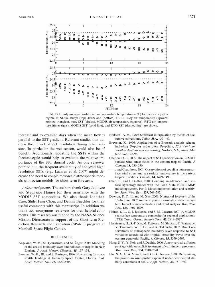
Comparison of the simulated and buoy 2-m air tem-peratures (Fig. 23) indicates that the model differencesare smaller than the difference between the models andthe buoys. During the night, the models show a similarcooling trend when compared to the buoys, however,during the day, the model air temperature either re-mains nearly constant (41010) or continues to decrease(41009), missing the diurnal cycle seen in the buoy ob-servations. The Eta Model forcing indicates cold advec-tion along the eastern boundary of the model domain(not shown), which can be implied from the negativeair–sea temperature difference at NDBC buoy 41010.This discrepancy suggests that the model sensible heat

FIG. 21. Hourly averaged wind speeds (m s�1) for the easterly-flow regime at NDBC buoys(top) 41009 and (bottom) 41010. Buoy (upward-pointed triangle), buoy adjusted to 10 m(downward-pointed triangle), MODIS (square), and RTG (times sign) are shown.

TABLE 1. Comparison of composite WRF simulations with NDBC buoy wind speeds and wind speeds adjusted to a 10-m height foreasterly- (westerly-) flow regimes. Boldface values indicate the simulation that compared best to the 10-m wind speed estimates.

NDBC buoy LocationBuoy avg windspeed (m s�1)

Buoy avg windspeed at 10 m (m s�1)

RTG SSTwind speed

MODIS SSTwind speed

41008 31.40°N, 80.87°W 4.05 (6.45) 4.37 (6.97) 5.86 (8.17) 5.82 (8.28)41009 28.50°N, 80.17°W 6.74 (4.33) 7.27 (4.67) 7.54 (4.80) 7.46 (4.70)41010 28.95°N, 78.47°W 7.00 (4.82) 7.56 (5.21) 6.64 (5.01) 6.69 (5.08)41012 30.00°N, 80.60°W 5.07 (5.14) 5.48 (5.55) 6.91 (6.41) 6.64 (6.41)


flux may be to low for both the MODIS and RTGsimulations.

5. Summary and conclusions

In this study, parallel simulations were studied to de-termine the impact of high-resolution SSTs on short-

term forecasts in the Florida region. The simulationsused either the RTG SST analysis or the 1-km MODISSST composite as a lower boundary condition for a 24-hWRF forecast. RUC analyses, surface, and upper-airobservations were assimilated using ADAS, providingthe initial conditions for the WRF. Two simulationswere performed for each day during May 2004. Resultsfocused on the impact of the simulations within theMABL. A unique aspect of this study, which is in con-trast to previous work (e.g., Song et al. 2006), is therealistic nature of the modeled SST. The modificationsto the SST here are complex as opposed to idealizedadjustments (step function changes, gradient versus nogradient, etc.).

The impact of the high-resolution MODIS SST com-posite was observable through a comparison of indi-vidual simulations, including earlier onset and morevigorous HCRs, elongated/more intense zones of con-vergence, and an increase in precipitation. Aggregatesof model output were used to evaluate the impact ofhigh-resolution SSTs in easterly and westerly domi-nated low-level flow. Surface heat flux changes associ-ated with the use of the MODIS SST product weredirectly correlated to SST changes between the SSTproducts. Upward sensible heat fluxes over the FloridaCurrent were larger with the MODIS SST product,while enhanced downward sensible heat fluxes oc-curred over the cooler waters of the Florida–Hatterasshelf. Vertical wind stress divergence and pressure gra-dient accelerations across the Florida Current regionvary in importance as a function of flow direction andstability. The most significant increase in surface windsin the MODIS simulations occurred during the stablewesterly flow regime, with vertical wind stress diver-gence being the dominant factor. In particular, our re-sults along SST gradient regions in easterly flow simu-lations are influenced by the significant heat contentadded upwind. The relative importance of the pressuregradient forcing throughout the MABL in this study isinfluenced by this effect. The warmer Florida Currentpresent in the MODIS product results in enhanced ver-tical heat transport that is advected downwind, modi-fying the thermal structure (e.g., boundary layer depth)and the MABL wind field primarily through pressuregradient adjustments. The adjustments are carried upand over the cooler shelf waters in the easterly flowsimulations. The deeper mixed layer in the easterly flowcases yields a response to the surface forcing that is moreextensive in the vertical. Validation of the WRF runs withbuoy and TMI data indicated that the use of the higher-resolution SST product led to small improvements.

Future work can be extended to investigate the im-pact of the MODIS SST composites on the daytime

FIG. 22. (a) TMI wind speed average (m s�1) for the period of10–19 May 2004. (Data courtesy of Remote Sensing Systems,Santa Rosa, CA.) (b) WRF MODIS run average wind speed forthe easterly-flow-regime cases: 9, 11–19 May 2004. The hatchedline represents a relative maximum in wind speed not observed inthe TMI data.


forecast and to examine days when the mean flow isparallel to the SST gradient. Relevant studies that ad-dress the impact of SST resolution during other sea-sons, in particular the wet season, would also be ofbenefit. Additionally, updating the SSTs within theforecast cycle would help to evaluate the relative im-portance of the SST diurnal cycle. As one reviewerpointed out, the frequent availability of analyzed high-resolution SSTs (e.g., Lazarus et al. 2007) might de-crease the need to couple mesoscale atmospheric mod-els with ocean models for short-term forecasts.

Acknowledgments. The authors thank Gary Jedlovecand Stephanie Haines for their assistance with theMODIS SST composites. We also thank JonathanCase, Shih-Hung Chou, and Dennis Buechler for theiruseful comments with this manuscript. In addition wethank two anonymous reviewers for their helpful com-ments. This research was funded by the NASA ScienceMission Directorate in support of the Short-term Pre-diction Research and Transition (SPoRT) program atMarshall Space Flight Center.

REFERENCES

Angevine, W. M., M. Tjernström, and M. Žagar, 2006: Modelingof the coastal boundary layer and pollutant transport in NewEngland. J. Appl. Meteor. Climatol., 45, 137–154.

Bauman, W. H., III, and S. Businger, 1996: Nowcasting for spaceshuttle landings at Kennedy Space Center, Florida. Bull.Amer. Meteor. Soc., 77, 2295–2305.

Bratseth, A. M., 1986: Statistical interpolation by means of suc-cessive corrections. Tellus, 38A, 439–447.

Brewster, K., 1996: Application of a Bratseth analysis schemeincluding Doppler radar data. Preprints, 15th Conf. onWeather Analysis and Forecasting, Norfolk, VA, Amer. Me-teor. Soc., 92–95.

Chelton, D. B., 2005: The impact of SST specification on ECMWFsurface wind stress fields in the eastern tropical Pacific. J.Climate, 18, 530–550.

——, and Coauthors, 2001: Observations of coupling between sur-face wind stress and sea surface temperature in the easterntropical Pacific. J. Climate, 14, 1479–1498.

Chen, F., and J. Dudhia, 2001: Coupling an advanced land sur-face–hydrology model with the Penn State–NCAR MM5modeling system. Part I: Model implementation and sensitiv-ity. Mon. Wea. Rev., 129, 569–585.

Dawson, D. T., II, and M. Xue, 2006: Numerical forecasts of the15–16 June 2002 southern plains mesoscale convective sys-tem: Impact of mesoscale data and cloud analysis. Mon. Wea.Rev., 134, 1607–1629.

Haines, S. L., G. J. Jedlovec, and S. M. Lazarus, 2007: A MODISsea surface temperature composite for regional applications.IEEE Trans. Geosci. Remote Sens., 45, 2919–2927.

Hashizume, H., S.-P. Xie, M. Fujiwara, M. Shiotani, T. Watanabe,Y. Tanimoto, W. T. Liu, and K. Takeuchi, 2002: Direct ob-servations of atmospheric boundary layer response to SSTvariations associated with tropical instability waves over theeastern equatorial Pacific. J. Climate, 15, 3379–3393.

Hong, S.-Y., Y. Noh, and J. Dudhia, 2006: A new vertical diffusionpackage with an explicit treatment of entrainment processes.Mon. Wea. Rev., 134, 2318–2341.

Hsu, S. A., E. A. Meindl, and D. B. Gilhousen, 1994: Determiningthe power-law wind-profile exponent under near-neutral sta-bility conditions at sea. J. Appl. Meteor., 33, 757–765.

FIG. 23. Hourly averaged surface air and sea surface temperatures (°C) for the easterly-flowregime at NDBC buoys (top) 41009 and (bottom) 41010. Buoy air temperature (upward-pointed triangles), buoy SST (circles), MODIS air temperature (squares), RTG air tempera-ture (times signs), MODIS SST (solid line), and RTG SST (dashed line) are shown.


Janjic, Z. I., 1994: The step-mountain Eta coordinate model: Fur-ther developments of the convection, viscous sublayer, andturbulence closure schemes. Mon. Wea. Rev., 122, 927–945.

Koracin, D., and D. P. Rogers, 1990: Numerical simulations of theresponse of the marine atmosphere to ocean forcing. J. At-mos. Sci., 47, 592–611.

Lazarus, S. M., C. M. Ciliberti, J. D. Horel, and K. A. Brewster,2002: Near-real-time applications of a mesoscale analysis sys-tem to complex terrain. Wea. Forecasting, 17, 971–1000.

——, C. G. Calvert, M. E. Splitt, P. Santos, D. W. Sharp, P. F.Blottman, and S. M. Spratt, 2007: Real-time, high-resolution,space–time analysis of sea surface temperatures from mul-tiple platforms. Mon. Wea. Rev., 135, 3158–3173.

Lericos, T. P., H. E. Fuelberg, A. I. Watson, and R. L. Holle, 2002:Warm season lightning distributions over the Florida peninsulaas related to synoptic patterns. Wea. Forecasting, 17, 83–98.

Li, X., W. Zheng, W. G. Pichel, C.-Z. Zou, P. Clemente-Colón,and K. S. Friedman, 2004: A cloud line over the Gulf Stream.Geophys. Res. Lett., 31, L14108, doi:10.1029/2004GL019892.

Lindzen, R. S., and S. Nigam, 1987: On the role of sea surfacetemperature gradients in forcing low-level winds and conver-gence in the Tropics. J. Atmos. Sci., 44, 2418–2436.

Lorenc, A. C., 1995: Atmospheric data assimilation. Met Office,Scientific Paper 34, 17 pp.

Maloney, E. D., and D. B. Chelton, 2006: An assessment of thesea surface temperature influence on surface wind stress innumerical weather prediction and climate models. J. Climate,19, 2743–2762.

Mellor, G. L., and T. Yamada, 1982: Development of a turbulenceclosure model for geophysical fluid problems. Rev. Geophys.Space Phys., 20, 851–875.

Minnett, P. J., 2003: Radiometric measurements of the sea-surfaceskin temperature: The competing roles of the diurnal ther-mocline and the cool skin. Int. J. Remote Sens., 24, 5033–5047.

——, R. H. Evans, O. Brown, E. Key, G. Szczodrak, K. Kilpatrick,W. Baringer, and S. Walsh, cited 2007: MODIS sea-surfacetemperatures for GHRSST-PP. Preprints, GHRSST-PP SixthScience Team Meeting, Exeter, United Kingdom, Met Office.[Available online at http://ghrsst-pp.metoffice.com/pages/meetings/workshop6/Presentations/19th/Minnett-Evans-RSMAS_GHRSST6_200519-release.ppt.]

NCDC, cited 2004: Climate of 2004—May Florida drought.[Available online at http://www.ncdc.noaa.gov/oa/climate/research/2004/may/st008dv00pcp200405.html.]

Nonaka, M., and S.-P. Xie, 2003: Covariations of sea surface tem-perature and wind over the Kuroshio and its extension: Evi-dence for ocean-to-atmosphere feedback. J. Climate, 16,1404–1413.

O’Neill, L. W., D. B. Chelton, and S. K. Esbensen, 2003: Obser-vations of SST-induced perturbations of the wind stress fieldover the Southern Ocean on seasonal timescales. J. Climate,16, 2340–2354.

——, ——, ——, and F. J. Wentz, 2005: High-resolution satellitemeasurements of the atmospheric boundary layer response toSST variations along the Agulhas Return Current. J. Climate,18, 2706–2723.

Raman, S., N. C. Reddy, and D. S. Niyogi, 1998: Mesoscale analysisof a Carolina coastal front. Bound.-Layer Meteor., 86, 125–145.

Rouault, M., A. M. Lee-Thorp, and J. R. E. Lutjeharms, 2000: Theatmospheric boundary layer above the Agulhas Current dur-ing alongcurrent winds. J. Phys. Oceanogr., 30, 40–50.

——, C. J. C. Reason, J. R. E. Lutjeharms, and A. C. M. Beljaars,2003: Underestimation of latent and sensible heat fluxes

above the Agulhas Current in NCEP and ECMWF analyses.J. Climate, 16, 776–782.

Samelson, R. M., E. D. Skyllingstad, D. B. Chelton, S. K. Es-bensen, L. W. O’Neill, and N. Thum, 2006: On the couplingof wind stress and sea surface temperature. J. Climate, 19,1557–1566.

Skamarock, W. C., J. B. Klemp, J. Dudhia, D. O. Gill, D. M.Barker, W. Wang, and J. G. Powers, 2005: A description ofthe advanced research WRF version 2. NCAR Tech. NoteNCAR/TN-468� STR, 88 pp.

Skyllingstad, E. D., R. M. Samelson, L. Mahrt, and P. Barbour,2005: A numerical modeling study of warm offshore flowover cool water. Mon. Wea. Rev., 133, 345–361.

Small, R. J., S.-P. Xie, and Y. Wang, 2003: Numerical simulationof atmospheric response to Pacific tropical instability waves.J. Climate, 16, 3723–3741.

Song, Q., T. Hara, P. Cornillon, and C. A. Friehe, 2004: A com-parison between observations and MM5 simulations of themarine atmospheric boundary layer across a temperaturefront. J. Atmos. Oceanic Technol., 21, 170–178.

——, P. Cornillon, and T. Hara, 2006: Surface wind response tooceanic fronts. J. Geophys. Res., 111, C12006, doi:10.1029/2006JC003680.

Sublette, M. S., and G. S. Young, 1996: Warm-season effects ofthe Gulf Stream on mesoscale characteristics of the atmo-spheric boundary layer. Mon. Wea. Rev., 124, 653–667.

Thiébaux, J., E. Rogers, W. Wang, and B. Katz, 2003: A newhigh-resolution blended real-time global sea surface tempera-ture analysis. Bull. Amer. Meteor. Soc., 84, 645–656.

Tijm, A. B. C., A. A. M. Holtslag, and A. J. van Delden, 1999:Observations and modeling of the sea breeze with the returncurrent. Mon. Wea. Rev., 127, 625–640.

Tokinaga, H., Y. Tanimoto, and S.-P. Xie, 2005: SST-induced sur-face wind variations over the Brazil–Malvinas confluence:Satellite and in situ observations. J. Climate, 18, 3470–3482.

——, and Coauthors, 2006: Atmospheric sounding over the winterKuroshio Extension: Effect of surface stability on atmo-spheric boundary layer structure. Geophys. Res. Lett., 33,L04703, doi:10.1029/2005GL025102.

Troen, I. B., and L. Mahrt, 1986: A simple model of the atmo-spheric boundary layer; sensitivity to surface evaporation.Bound.-Layer Meteor., 37, 129–148.

Wallace, J. M., T. P. Mitchell, and C. Deser, 1989: The influenceof sea-surface temperature on surface wind in the easternequatorial Pacific: Seasonal and interannual variability. J.Climate, 2, 1492–1499.

Warner, T. T., M. N. Lakhtakia, J. D. Doyle, and R. A. Pearson,1990: Marine atmospheric boundary layer circulations forcedby Gulf Stream sea surface temperature gradients. Mon.Wea. Rev., 118, 309–323.

Xue, M., and W. J. Martin, 2006: A high-resolution modelingstudy of the 24 May 2002 dryline case during IHOP. Part I:Numerical simulation and general evolution of the drylineand convection. Mon. Wea. Rev., 134, 149–171.

——, K. K. Droegemeier, and V. Wong, 2000: The Advanced Re-gional Prediction Systems (ARPS)—A multi-scale nonhydro-static atmospheric simulation and prediction model. Part I:Model dynamics and verification. Meteor. Atmos. Phys., 75,161–193.

Zhang, F., A. M. Odins, and J. W. Nielsen-Gammon, 2006: Me-soscale predictability of an extreme warm-season precipita-tion event. Wea. Forecasting, 21, 149–166.


Documents

The Impact of High-Resolution Sea Surface Temperatures …weather.msfc.nasa.gov/sport/journal/pdfs/2008_MWR_LaCasse_etal.pdf · The Impact of High-Resolution Sea Surface Temperatures