ORIGINAL PAPER

The impact of geological uncertainty on primary productionfrom a fluvial reservoir

Mohammad Koneshloo1 • Saman A. Aryana1,2 • Xiaoni Hu3

Received: 4 July 2017 / Published online: 21 April 2018� The Author(s) 2018

AbstractDeposition of fluvial sandbodies is controlled mainly by characteristics of the system, such as the rate of avulsion and

aggradation of the fluvial channels and their geometry. The impact and the interaction of these parameters have not

received adequate attention. In this paper, the impact of geological uncertainty resulting from the interpretation of the

fluvial geometry, maximum depth of channels, and their avulsion rates on primary production is studied for fluvial

reservoirs. Several meandering reservoirs were generated using a process-mimicking package by varying several con-

trolling factors. Simulation results indicate that geometrical parameters of the fluvial channels impact cumulative pro-

duction during primary production more significantly than their avulsion rate. The most significant factor appears to be the

maximum depth of fluvial channels. The overall net-to-gross ratio is closely correlated with the cumulative oil production

of the field, but cumulative production values for individual wells do not appear to be correlated with the local net-to-gross

ratio calculated in the vicinity of each well. Connectedness of the sandbodies to each well, defined based on the minimum

time-of-flight from each block to the well, appears to be a more reliable indicator of well-scale production.

Keywords Geological uncertainty evaluation � Fluvial reservoir modeling � Process-mimicking simulation �Geometry of fluvial channels

1 Introduction

Fluvial reservoirs are heterogeneous at a multitude of

scales. High-permeability contrasts between mud and sand

deposits make the connectivity of sandbodies the main

controlling factor for reservoir quality. The internal struc-

tures of sediments on a small scale (core and pore scales)

and stratigraphic correlation of fluvial formations on a

large scale have received more attention than the archi-

tecture of depositions, the geometry of channels, and

conserved sandbodies, which are more important for the

geological modeling of a reservoir (Gibling 2006). The

sources of geological uncertainty are classified by Mas-

sonnat (2000) in a six-level hierarchical chart: data

acquisition, interpretation of data, geological concept

elaboration, the spatial distribution of geological features,

choice of the input parameters, and generation of

equiprobable realizations. Despite the importance of these

factors, geological models are assumed fixed or predeter-

mined in many routine industrial appraisal projects, and

practitioners often prefer to focus only on one fine geo-

logical model and to analyze only the impact of dynamic

parameters. Laure and Hovadik (2008) state two reasons

for this lack of attention; first, it is believed that reservoir

architecture is a less important factor in oil production than

other petrophysical and fluid properties or the operational

parameters of a reservoir. Second, generating realistic

subsurface models is a difficult and time-consuming task.

In fact, the first reason may be true only if the lithological

facies demonstrate similar patterns or exhibit similar con-

nectivity despite their different patterns. The difficulty of

subsurface modeling resides in its uncertain nature coming

from lack of subsurface data which lead to various possible

Edited by Jie Hao

& Mohammad Koneshloo

mkoneshl@uwyo.edu

1 Department of Petroleum Engineering, University of

Wyoming, Laramie, WY 87061, USA

2 Department of Chemical Engineering, University of

Wyoming, Laramie, WY 87061, USA

3 Department of Geological Sciences, University of Wyoming,

Laramie, WY 87061, USA

123

Petroleum Science (2018) 15:270–288https://doi.org/10.1007/s12182-018-0229-y(0123456789().,-volV)(0123456789().,-volV)

interpretations of the geological settings, where the sedi-

mentological and structural factors are thought to be the

major sources of uncertainty. A specific geological model,

however, can never capture the full range of geological

uncertainty of a reservoir (Caumon and Journel 2005).

Fluvial reservoirs and especially meandering deposits

appear to demonstrate the importance of reservoir archi-

tecture in project appraisal. The architecture of the mean-

dering deposits, formed by multi-story channel deposits

separated by floodplain mud, is complex as a result of

lateral migration and avulsion. The sand fraction is known

as the dominant factor in evaluation of a fluvial reservoir,

while the geometry of channels, avulsion rate, and direc-

tion of point-bar migration are also significant (Jones et al.

2009). These factors also determine the connectivity of

sandbodies (high permeable regions), which is a dominant

factor influencing fluid flow and shaping preferential flow

pathways in reservoirs (Pranter and Sommer 2011). All of

these characteristics are controlled by the geological

parameters of the system. Correct estimation of sandbodies

and their topological relationships are key elements in

understanding these reservoirs. This paper aims to

demonstrate the impact of the geometry of fluvial channels

and avulsion rates on the quality of a fluvial reservoir.

Numerical reservoir modeling is a commonly used tool

for analyzing the impact of geological features on pro-

duction. Most stochastic reservoir modeling methods rely

on spatial correlation and well data to generate represen-

tative models. In such a framework, it is difficult to

incorporate physical laws of sedimentation and prevent

geologically incorrect placement of sandbodies (Tye 2013).

Methods such as object-based methods (Pyrcz and Deutsch

2014) and multiple-point geostatistics (Strebelle 2002;

Rezaee et al. 2013) rely on predefined patterns or objects,

which are the consequence of sedimentation under a

defined set of geological factors. Process-based simulators

are tools developed to mimic the sedimentation process and

to evaluate the impact of geological factors directly (De-

viese 2010; Hajek and Wolinsky 2012). Most process-

based simulators incorporate a simplified equation of flow

to mimic processes governing deposition of sediments

(Cojan et al. 2005). In this study, subsurface models are

generated using FLUMY, a process-mimicking software

for meandering systems (Koneshloo et al. 2017).

This work focuses on levels three and four of the

Massonnat (2000) hierarchical classification of the sources

of uncertainty: elaboration of the geological model and

explanation of the main factors controlling the distribution

of the geological features in a meandering reservoir.

According to Tye (2013), the most important factors con-

trolling the static connectivity of sedimentary sandbodies

are channel widths and net-to-gross ratio (NGR) values.

Although NGR values calculated using well data (1-D) are

generally used as acceptable approximations of the reser-

voir NGR, the interpretation of the shape and lateral

extension of sedimentary features solely based on vertical

data is rather difficult. In this work, several models are

generated to study the impact of uncertainty inherent in

subsurface model conceptualization and the controlling

factors. The following sections describe the geometry of

channels, present several empirical equations used to

explain the geometry of channels, and discuss ambiguities

in their application. Petrophysical models are generated,

and oil production from each model is simulated. Field-

level and well-level results are compared, and the impact of

various geological factors on cumulative primary produc-

tion is analyzed.

2 Materials and methods

In geometrical modeling of a reservoir’s features, we are

often faced with a scarcity of data. Three-dimensional

seismic data are often used to generate pseudo-images of

the subsurface. Several studies show that incised valleys,

channel belts, large channels (with a thickness above the

seismic vertical resolution), and abandoned channels filled

with coaly horizons are seismically detectable (Alsouki

et al. 2014; Zhang et al. 2015). In the absence of seismic

data, outcrops and modern deposition systems are impor-

tant sources of information related to sedimentary features.

For a given reservoir, architecture dictates the spatial dis-

tribution of reservoir properties within the reservoir. The

distinction between all sedimentological features and reli-

able estimation of their geometrical parameters are not

always possible. Although core and log data have good

vertical resolutions, lateral continuity cannot be extracted

directly from such data.

Miall (2014) illustrates the uncertainty inherent in geo-

logical modeling using three interpreted sections of zone

one of the Travis Peak Formation. In this study, three

different empirical equations are used to estimate channel

widths based on their depths (Bridge and Mackey 2009;

Leeder 1973; Williams 1986). Due to differences in

assumptions, the same logs result in three completely dif-

ferent representations of the subsurface in terms of the

connectivity of sandbodies. Additional challenges include

synonymous use of terms (e.g., meander belt and channel)

and inconsistent estimation of influential parameters (e.g.,

width of fluvial channels may be estimated based on either

maximum bankfull depth, or mean bankfull depth of the

channels, or thickness of sandbodies). Finally, these vari-

ables must often be inferred based on limited one-dimen-

sional data. Table 1 shows the most commonly used

empirical equations for the estimation of lateral extension

Petroleum Science (2018) 15:270–288 271

123

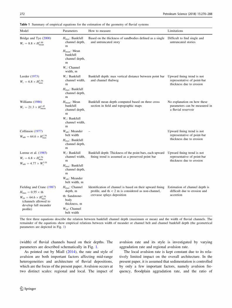
(width) of fluvial channels based on their depths. The

parameters are described schematically in Fig. 1.

As pointed out by Miall (2014), the rate and style of

avulsion are both important factors affecting mid-range

heterogeneities and architecture of fluvial depositions,

which are the focus of the present paper. Avulsion occurs at

two distinct scales: regional and local. The impact of

avulsion rate and its style is investigated by varying

aggradation rate and regional avulsion rate.

The local avulsion rate is kept constant due to its rela-

tively limited impact on the overall architecture. In the

present paper, it is assumed that sedimentation is controlled

by only a few important factors, namely avulsion fre-

quency, floodplain aggradation rate, and the ratio of

Table 1 Summary of empirical equations for the estimation of the geometry of fluvial systems

Model Parameters How to measure Limitations

Bridge and Tye (2000)

Wc ¼ 8:8� H1:88mean

Hmax: Bankfull

channel depth,

m

Hmean: Mean

bankfull

channel depth,

m

Wc: Channel

width, m

Based on the thickness of sandbodies defined as a single

and untruncated story

Difficult to find single and

untruncated stories

Leeder (1973)

Wc ¼ 6:8� H1:54max

Wc: Bankfull

channel width,

m

Hmax: Bankfull

channel depth,

m

Bankfull depth: max vertical distance between point bar

and channel thalweg

Upward fining trend is not

representative of point-bar

thickness due to erosion

Williams (1986)

Wc ¼ 21:3� H1:45mean

Hmean: Mean

bankfull

channel depth,

m

Wc: Bankfull

channel width,

m

Bankfull mean depth computed based on three cross

section in field and topographic maps

No explanation on how these

parameters can be measured in

a fluvial reservoir

Collinson (1977)

Wmb ¼ 64:6� H1:54max

Wmb: Meander

belt width

Hmax: Bankfull

channel depth,

m

– Upward fining trend is not

representative of point-bar

thickness due to erosion

Lorenz et al. (1985)

Wc ¼ 6:8� H1:54max

Wmb ¼ 4:77�W1:01c

Wc: Bankfull

channel width,

m

Hmax: Bankfull

channel depth,

m

Wmb: Meander

belt width, m

Bankfull depth: Thickness of the point bars, each upward

fining trend is assumed as a preserved point bar

Upward fining trend is not

representative of point-bar

thickness due to erosion

Fielding and Crane (1987)

Hmax ¼ 0:55� th

Wcb ¼ 64:6� H1:54max

(channels allowed to

develop full meander

profile)

Hmax: Channel

depth, m

th: Sandstone-

body

thickness, m

Wcb: Channel

belt width

Identification of channel is based on their upward fining

profile, and th\ 2 m is considered as non-channel,

crevasse splays deposition

Estimation of channel depth is

difficult due to erosion and

accretion

The first three equations describe the relation between bankfull channel depth (maximum or mean) and the width of fluvial channels. The

remainder of the equations show empirical relations between width of meander or channel belt and channel bankfull depth (the geometrical

parameters are depicted in Fig. 1)

272 Petroleum Science (2018) 15:270–288

123

channel belt or of floodplain to the width in the stacking of

channel bodies.

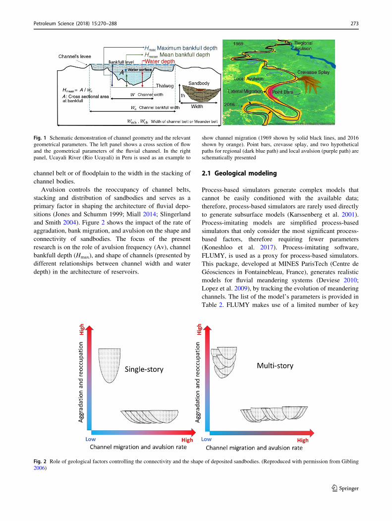
Avulsion controls the reoccupancy of channel belts,

stacking and distribution of sandbodies and serves as a

primary factor in shaping the architecture of fluvial depo-

sitions (Jones and Schumm 1999; Miall 2014; Slingerland

and Smith 2004). Figure 2 shows the impact of the rate of

aggradation, bank migration, and avulsion on the shape and

connectivity of sandbodies. The focus of the present

research is on the role of avulsion frequency (Av), channel

bankfull depth (Hmax), and shape of channels (presented by

different relationships between channel width and water

depth) in the architecture of reservoirs.

2.1 Geological modeling

Process-based simulators generate complex models that

cannot be easily conditioned with the available data;

therefore, process-based simulators are rarely used directly

to generate subsurface models (Karssenberg et al. 2001).

Process-imitating models are simplified process-based

simulators that only consider the most significant process-

based factors, therefore requiring fewer parameters

(Koneshloo et al. 2017). Process-imitating software,

FLUMY, is used as a proxy for process-based simulators.

This package, developed at MINES ParisTech (Centre de

Geosciences in Fontainebleau, France), generates realistic

models for fluvial meandering systems (Deviese 2010;

Lopez et al. 2009), by tracking the evolution of meandering

channels. The list of the model’s parameters is provided in

Table 2. FLUMY makes use of a limited number of key

Fig. 1 Schematic demonstration of channel geometry and the relevant

geometrical parameters. The left panel shows a cross section of flow

and the geometrical parameters of the fluvial channel. In the right

panel, Ucayali River (Rio Ucayali) in Peru is used as an example to

show channel migration (1969 shown by solid black lines, and 2016

shown by orange). Point bars, crevasse splay, and two hypothetical

paths for regional (dark blue path) and local avulsion (purple path) are

schematically presented

Fig. 2 Role of geological factors controlling the connectivity and the shape of deposited sandbodies. (Reproduced with permission from Gibling

2006)

Petroleum Science (2018) 15:270–288 273

123

parameters (fewer than what is needed for a process-based

model). The main controlling factors are regional avulsion

rate, aggradation rate, and general topography (slope of the

basin). In each iteration, FLUMY calculates migration of

the centerline; details are described in Cojan et al. (2005)

and Lopez et al. (2009). For each pixel, sediment will be

deposited according to its distance from the centerline. An

exponential function for distance from the centerline is

used to assign the grain size and the thickness of the sed-

iments during each iteration (Lauer and Parker 2008; Piz-

zuto et al. 2008).

In FLUMY, regional avulsion is defined as an avulsion

happening upstream of the domain and local avulsion

refers to a levee breach inside the domain. The frequency

of the local avulsion (levee breaches) and regional avul-

sion, and the aggradation rate of the floodplain used in this

study are specified Table 2. Other variables include the

equation used to relate channel width to channel depth,

avulsion periodicity (Av), and maximum channel depth

(Hmax).

A 3D model of a fluvial meandering system with

approximately 7 million cells (216 9 216 9 150) is sim-

ulated. This simulated field is 75 m thick, 3240 m wide,

and 3240 m long and is used as the reference model. Cell

dimensions are 0.5 m in the z-direction and 15 m in the x-

and y-directions. There are two possible sources of ran-

domness in FLUMY.

The first source is the randomness of the model’s

parameters, and the second source resides in the way the

algorithm has been designed to simulate the fluvial regime,

initial river path, and its new path caused by regional

avulsion. Parameters used in the generation of the reference

model are based on unit four of Schooner Field, as reported

by Deviese (2010). Lithological data are sampled along 16

vertical wells located approximately at centers of 80-acre

parcels in the reference model. Subsequently, fifty-four

geological models are generated using FLUMY, by varying

the maximum depth of the fluvial channel, the equation

used to estimate channel widths, and the avulsion rate.

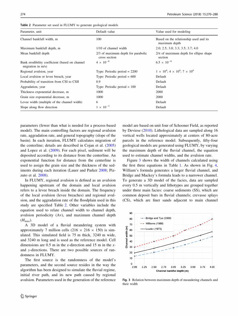
Figure 3 shows the width of channels calculated using

the first three equations in Table 1. As shown in Fig. 4,

William’s formula generates a larger fluvial channel, and

Bridge and Mackey’s formula leads to a narrower channel.

To generate a 3D model of the facies, data are sampled

every 0.5 m vertically and lithotypes are grouped together

under three main facies: coarse sediments (SS), which are

common deposit bars in fluvial channels; crevasse splays

(CS), which are finer sands adjacent to main channel

Fig. 3 Relation between maximum depth of meandering channels and

their width

Table 2 Parameter set used in FLUMY to generate geological models

Parameter, unit Default value Value used for modeling

Channel bankfull width, m 100 Based on the relationship used and its

maximum depth

Maximum bankfull depth, m 1/10 of channel width 2.0; 2.5; 3.0; 3.3; 3.5; 3.7; 4.0

Mean bankfull depth 2/3 of maximum depth for parabolic

cross section

2/p of maximum depth for ellipse shape

section

Bank erodibility coefficient (based on channel

migration in m/s)

4 9 10-8 6.5 9 10-8

Regional avulsion, year Type: Periodic period = 2200 1 9 104; 4 9 104; 7 9 104

Local avulsion or levee breach, year Type: Periodic period = 600 Default

Probability of transition from CSI to CSII 0.9 Default

Aggradation, year Type: Periodic period = 100 Default

Thickness exponential decrease, m 1000 2000

Grain size exponential decrease, m 1000 2000

Levee width (multiple of the channel width) 6 Default

Slope along flow direction 1 9 10-3 Default

274 Petroleum Science (2018) 15:270–288

123

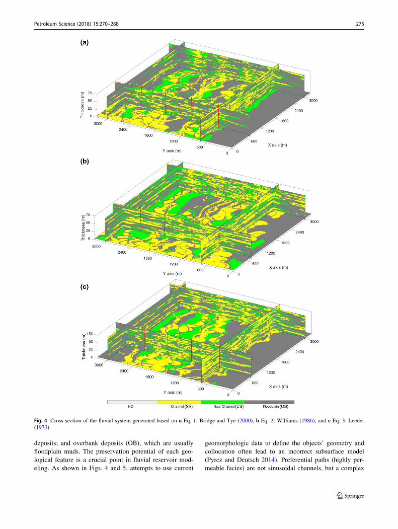
deposits; and overbank deposits (OB), which are usually

floodplain muds. The preservation potential of each geo-

logical feature is a crucial point in fluvial reservoir mod-

eling. As shown in Figs. 4 and 5, attempts to use current

geomorphologic data to define the objects’ geometry and

collocation often lead to an incorrect subsurface model

(Pyrcz and Deutsch 2014). Preferential paths (highly per-

meable facies) are not sinusoidal channels, but a complex

Fig. 4 Cross section of the fluvial system generated based on a Eq. 1: Bridge and Tye (2000), b Eq. 2: Williams (1986), and c Eq. 3: Leeder

(1973)

Petroleum Science (2018) 15:270–288 275

123

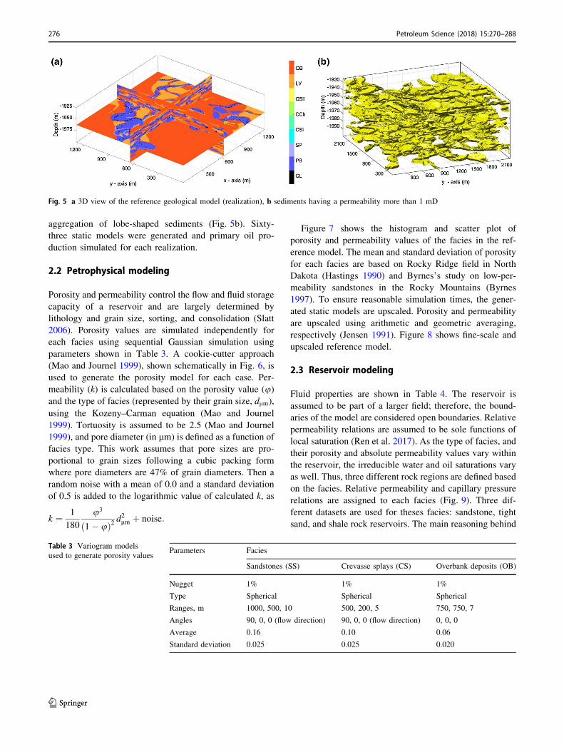
aggregation of lobe-shaped sediments (Fig. 5b). Sixty-

three static models were generated and primary oil pro-

duction simulated for each realization.

2.2 Petrophysical modeling

Porosity and permeability control the flow and fluid storage

capacity of a reservoir and are largely determined by

lithology and grain size, sorting, and consolidation (Slatt

2006). Porosity values are simulated independently for

each facies using sequential Gaussian simulation using

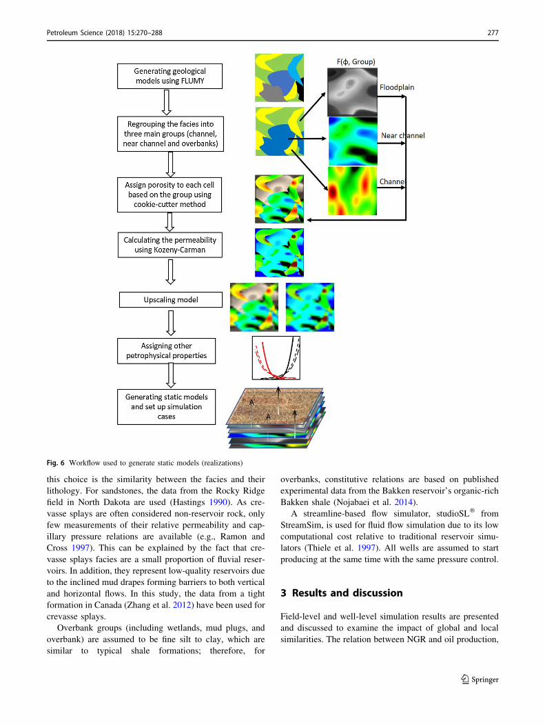
parameters shown in Table 3. A cookie-cutter approach

(Mao and Journel 1999), shown schematically in Fig. 6, is

used to generate the porosity model for each case. Per-

meability (k) is calculated based on the porosity value (u)and the type of facies (represented by their grain size, dlm),

using the Kozeny–Carman equation (Mao and Journel

1999). Tortuosity is assumed to be 2.5 (Mao and Journel

1999), and pore diameter (in lm) is defined as a function of

facies type. This work assumes that pore sizes are pro-

portional to grain sizes following a cubic packing form

where pore diameters are 47% of grain diameters. Then a

random noise with a mean of 0.0 and a standard deviation

of 0.5 is added to the logarithmic value of calculated k, as

k ¼ 1

180

u3

1� uð Þ2d2lm þ noise:

Figure 7 shows the histogram and scatter plot of

porosity and permeability values of the facies in the ref-

erence model. The mean and standard deviation of porosity

for each facies are based on Rocky Ridge field in North

Dakota (Hastings 1990) and Byrnes’s study on low-per-

meability sandstones in the Rocky Mountains (Byrnes

1997). To ensure reasonable simulation times, the gener-

ated static models are upscaled. Porosity and permeability

are upscaled using arithmetic and geometric averaging,

respectively (Jensen 1991). Figure 8 shows fine-scale and

upscaled reference model.

2.3 Reservoir modeling

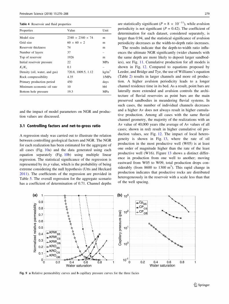
Fluid properties are shown in Table 4. The reservoir is

assumed to be part of a larger field; therefore, the bound-

aries of the model are considered open boundaries. Relative

permeability relations are assumed to be sole functions of

local saturation (Ren et al. 2017). As the type of facies, and

their porosity and absolute permeability values vary within

the reservoir, the irreducible water and oil saturations vary

as well. Thus, three different rock regions are defined based

on the facies. Relative permeability and capillary pressure

relations are assigned to each facies (Fig. 9). Three dif-

ferent datasets are used for theses facies: sandstone, tight

sand, and shale rock reservoirs. The main reasoning behind

Fig. 5 a 3D view of the reference geological model (realization), b sediments having a permeability more than 1 mD

Table 3 Variogram models

used to generate porosity valuesParameters Facies

Sandstones (SS) Crevasse splays (CS) Overbank deposits (OB)

Nugget 1% 1% 1%

Type Spherical Spherical Spherical

Ranges, m 1000, 500, 10 500, 200, 5 750, 750, 7

Angles 90, 0, 0 (flow direction) 90, 0, 0 (flow direction) 0, 0, 0

Average 0.16 0.10 0.06

Standard deviation 0.025 0.025 0.020

276 Petroleum Science (2018) 15:270–288

123

this choice is the similarity between the facies and their

lithology. For sandstones, the data from the Rocky Ridge

field in North Dakota are used (Hastings 1990). As cre-

vasse splays are often considered non-reservoir rock, only

few measurements of their relative permeability and cap-

illary pressure relations are available (e.g., Ramon and

Cross 1997). This can be explained by the fact that cre-

vasse splays facies are a small proportion of fluvial reser-

voirs. In addition, they represent low-quality reservoirs due

to the inclined mud drapes forming barriers to both vertical

and horizontal flows. In this study, the data from a tight

formation in Canada (Zhang et al. 2012) have been used for

crevasse splays.

Overbank groups (including wetlands, mud plugs, and

overbank) are assumed to be fine silt to clay, which are

similar to typical shale formations; therefore, for

overbanks, constitutive relations are based on published

experimental data from the Bakken reservoir’s organic-rich

Bakken shale (Nojabaei et al. 2014).

A streamline-based flow simulator, studioSL� from

StreamSim, is used for fluid flow simulation due to its low

computational cost relative to traditional reservoir simu-

lators (Thiele et al. 1997). All wells are assumed to start

producing at the same time with the same pressure control.

3 Results and discussion

Field-level and well-level simulation results are presented

and discussed to examine the impact of global and local

similarities. The relation between NGR and oil production,

Fig. 6 Workflow used to generate static models (realizations)

Petroleum Science (2018) 15:270–288 277

123

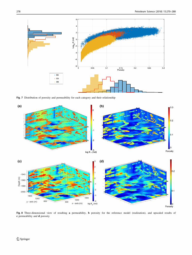
Fig. 7 Distribution of porosity and permeability for each category and their relationship

Fig. 8 Three-dimensional view of resulting a permeability, b porosity for the reference model (realization), and upscaled results of

c permeability and d porosity

278 Petroleum Science (2018) 15:270–288

123

and the impact of model parameters on NGR and produc-

tion values are discussed.

3.1 Controlling factors and net-to-gross ratio

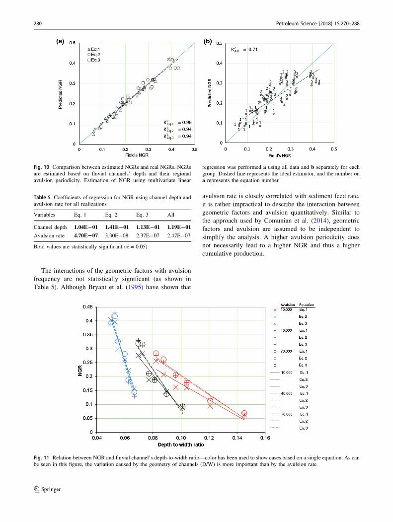
A regression study was carried out to illustrate the relation

between controlling geological factors and NGR. The NGR

for each realization has been estimated for the aggregate of

all cases (Fig. 10a) and the data generated using each

equation separately (Fig. 10b) using multiple linear

regression. The statistical significance of the regression is

represented by its p value, which is the probability of being

extreme considering the null hypothesis (Utts and Heckard

2011). The coefficients of the regression are provided in

Table 5. The overall regression for the aggregate scenario

has a coefficient of determination of 0.71. Channel depths

are statistically significant (P = 8 9 10-11), while avulsion

periodicity is not significant (P = 0.42). The coefficient of

determination for each dataset, considered separately, is

larger than 0.94, and the statistical significance of avulsion

periodicity decreases as the width-to-depth ratio increases.

The results indicate that the depth-to-width ratio influ-

ences the ultimate NGR significantly (wider channels with

the same depth are more likely to deposit larger sandbod-

ies), see Fig. 11. Cumulative production for all models is

shown in Fig. 12. Compared to equations proposed by

Leeder, and Bridge and Tye, the use of Williams’s equation

(Table 2) results in larger channels and more oil produc-

tion. A higher avulsion periodicity leads to a longer

channel residence time in its bed. As a result, point bars are

laterally more extended and avulsion controls the archi-

tecture of fluvial reservoirs as point bars are the main

preserved sandbodies in meandering fluvial systems. In

such cases, the number of individual channels decreases

and a higher Av does not always result in higher cumula-

tive production. Among all cases with the same fluvial

channel geometry, the majority of the realizations with an

Av value of 40,000 years (the average of Av values of all

cases; shown in red) result in higher cumulative oil pro-

duction values, see Fig. 12. The impact of local hetero-

geneity is shown in Fig. 13, where the rate of oil

production in the most productive well (W05) is at least

one order of magnitude higher than the rate of the least

productive well (W16). Figure 13 shows a distinct differ-

ence in production from one well to another; moving

eastward from W05 to W09, total production drops con-

siderably (from 8600 to 1300 m3). This rapid change in

production indicates that productive rocks are distributed

heterogeneously in the reservoir with a scale less than that

of the well spacing.

Fig. 9 a Relative permeability curves and b capillary pressure curves for the three facies

Table 4 Reservoir and fluid properties

Properties Value Unit

Model size 2340 9 2340 9 74 m

Grid size 60 9 60 9 2 m

Reservoir thickness 74 m

Number of layers 37 –

Top of reservoir 1926 m

Initial reservoir pressure 22 MPa

Kz/Kx 0.1 –

Density (oil, water, and gas) 720.8, 1009.5, 1.12 kg/m3

Rock compressibility 4.35 1/MPa

Primary production period 450 days

Minimum economic oil rate 10 bbl

Bottom hole pressure 19.3 MPa

Petroleum Science (2018) 15:270–288 279

123

The interactions of the geometric factors with avulsion

frequency are not statistically significant (as shown in

Table 5). Although Bryant et al. (1995) have shown that

avulsion rate is closely correlated with sediment feed rate,

it is rather impractical to describe the interaction between

geometric factors and avulsion quantitatively. Similar to

the approach used by Comunian et al. (2014), geometric

factors and avulsion are assumed to be independent to

simplify the analysis. A higher avulsion periodicity does

not necessarily lead to a higher NGR and thus a higher

cumulative production.

Fig. 10 Comparison between estimated NGRs and real NGRs. NGRs

are estimated based on fluvial channels’ depth and their regional

avulsion periodicity. Estimation of NGR using multivariate linear

regression was performed a using all data and b separately for each

group. Dashed line represents the ideal estimator, and the number on

a represents the equation number

Fig. 11 Relation between NGR and fluvial channel’s depth-to-width ratio—color has been used to show cases based on a single equation. As can

be seen in this figure, the variation caused by the geometry of channels (D/W) is more important than by the avulsion rate

Table 5 Coefficients of regression for NGR using channel depth and

avulsion rate for all realizations

Variables Eq. 1 Eq. 2 Eq. 3 All

Channel depth 1.04E201 1.41E201 1.13E201 1.19E201

Avulsion rate 4.70E207 3.30E-08 2.37E-07 2.47E-07

Bold values are statistically significant (a = 0.05)

280 Petroleum Science (2018) 15:270–288

123

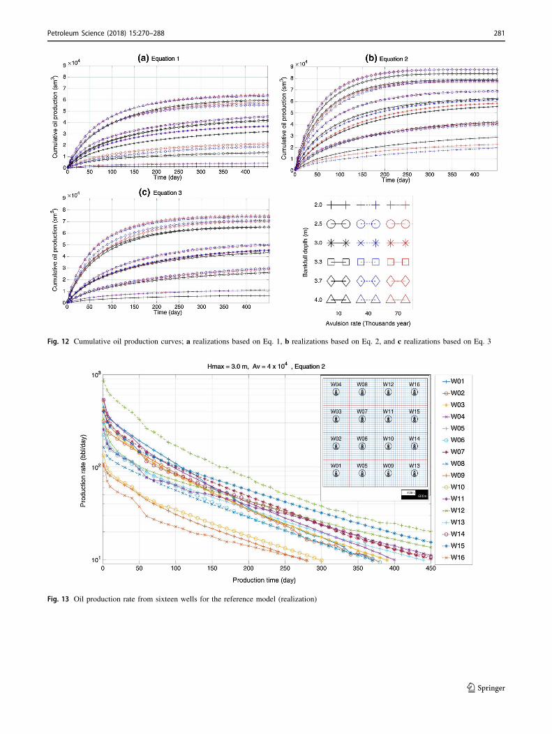
Fig. 12 Cumulative oil production curves; a realizations based on Eq. 1, b realizations based on Eq. 2, and c realizations based on Eq. 3

Fig. 13 Oil production rate from sixteen wells for the reference model (realization)

Petroleum Science (2018) 15:270–288 281

123

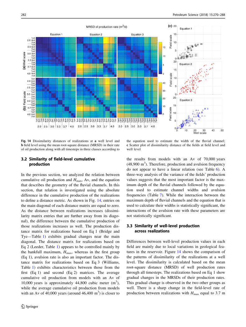
3.2 Similarity of field-level cumulativeproduction

In the previous section, we analyzed the relation between

cumulative oil production and Hmax, Av, and the equation

that describes the geometry of the fluvial channels. In this

section, that relation is investigated using the absolute

difference in the cumulative production of the realizations

to define a distance metric. As shown in Fig. 14, entries on

the main diagonal of each distance matrix are equal to zero.

As the distance between realizations increases (dissimi-

larity matrix entries that are further away from its diago-

nal), the difference between the cumulative production of

those realizations increases as well. The production dis-

tance matrix for realizations based on Eq 1 (Bridge and

Tye—Table 1) exhibits gradual changes near the main

diagonal. The distance matrix for realizations based on

Eq 2 (Leeder, Table 1) appears to be controlled mainly by

the bankfull maximum, Hmax, whereas in the first group

(Eq 1), avulsion rate is also an important factor. The dis-

tance matrix for realizations based on Eq 3 (Williams,

Table 1) exhibits characteristics between those from the

first (Eq 1) and second (Eq 2) matrices. The average

cumulative oil production from models with an Av of

10,000 years is approximately 44,800 cubic meter (m3),

while the average cumulative oil production from models

with an Av of 40,000 years (around 46,400 m3) is closer to

the results from models with an Av of 70,000 years

(48,900 m3). Therefore, production and avulsion frequency

do not appear to have a linear relation (see Table 6). A

three-way analysis of the variance of the fields’ production

values suggests that the most important factor is the max-

imum depth of the fluvial channels followed by the equa-

tion used to estimate channel widths and avulsion

frequencies (Table 7). While the interaction between the

maximum depth of fluvial channels and the equation that is

used to calculate their widths is statistically significant, the

interactions of the avulsion rate with these parameters are

not statistically significant.

3.3 Similarity of well-level productionacross realizations

Differences between well-level production values in each

field are mainly due to local variations in geological fea-

tures in the reservoir. Figure 14 shows the comparison of

the patterns of dissimilarity of the realizations at a well

level. The dissimilarity is calculated based on the mean

root-square distance (MRSD) of well production rates

through all timesteps. The realizations based on Eq 1 show

gradual changes in the MRSDs of their production rates.

This gradual change is observed in the two other groups as

well. There is a sharp change in the field-level rate of

production between realizations with Hmax equal to 3.7 m

Fig. 14 Dissimilarity distances of realizations at a well level and

b field level using the mean root-square distance (MRSD) in their rate

of oil production along with all timesteps in three classes according to

the equation used to estimate the width of the fluvial channel;

c Scatter plot of dissimilarity distance of the fields at field level and

well level

282 Petroleum Science (2018) 15:270–288

123

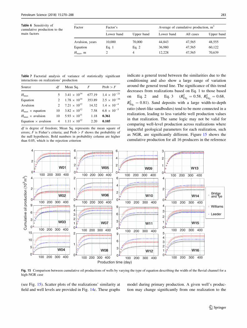
(see Fig. 15). Scatter plots of the realizations’ similarity at

field and well levels are provided in Fig. 14c. These graphs

indicate a general trend between the similarities due to the

conditioning and also show a large range of variation

around the general trend line. The significance of this trend

decreases from realizations based on Eq. 1 to those based

on Eq. 2 and Eq. 3 (R2Eq1

¼ 0:58; R2Eq2

¼ 0:68;

R2Eq3

¼ 0:81). Sand deposits with a large width-to-depth

ratio (sheet-like sandbodies) tend to be more connected in a

realization, leading to less variable well production values

in that realization. The same logic may not be valid for

comparing well-level production across realizations where

impactful geological parameters for each realization, such

as NGR, are significantly different. Figure 15 shows the

cumulative production for all 16 producers in the reference

model during primary production. A given well’s produc-

tion may change significantly from one realization to the

Fig. 15 Comparison between cumulative oil productions of wells by varying the type of equation describing the width of the fluvial channel for a

high-NGR case

Table 6 Sensitivity of

cumulative production to the

main factors

Factor Factor’s Average of cumulative production, m3

Lower band Upper band Lower band All cases Upper band

Avulsion, years 10,000 70,000 44,843 47,565 48,555

Equation Eq. 1 Eq. 2 36,980 47,565 60,122

Hmax, m 2 4 12,228 47,565 70,639

Table 7 Factorial analysis of variance of statistically significant

interactions on realizations’ production

Source df Mean Sq. F Prob[F

Hmax 5 3.41 9 1014 677.19 1.4 9 10-21

Equation 2 1.78 9 1014 353.89 2.5 9 10-16

Avulsion 2 7.21 9 1012 14.32 1.4 9 10-4

Hmax 9 equation 10 3.82 9 1012 7.58 6.8 9 10-5

Hmax 9 avulsion 10 5.93 9 1011 1.18 0.361

Equation 9 avulsion 4 1.11 9 1012 2.20 0.105

df is degree of freedom; Mean Sq. represents the mean square of

errors; F is Fisher’s criteria; and Prob[F shows the probability of

the null hypothesis. Bold numbers in probability column are higher

than 0.05, which is the rejection criterion

Petroleum Science (2018) 15:270–288 283

123

next, due to variations in the productive rocks’ proportion

in each parcel (80 acres around each well).

3.4 Net-to-gross ratio and cumulativeproduction

The net-to-gross ratio provides an approximation of the

reservoir quality and might be an indicator of the produc-

tive geobodies’ connectivity. Several authors have studied

the connectivity of sandbodies by varying the NGR, e.g.,

uniformly distributed sand packets (Allen 1979), Boolean

models and the truncated Gaussian method (Allard 1993),

and the object-based simulation method (Pranter and

Sommer 2011). In the present study, NGR is defined as the

volumetric proportion of sandbodies (channel lags, point

bars, and sand plugs and crevasses) to the total volume of

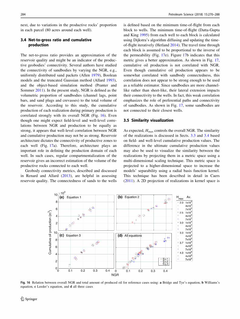
the reservoir. According to this study, the cumulative

production of each realization during primary production is

correlated strongly with its overall NGR (Fig. 16). Even

though one might expect field-level and well-level corre-

lations between NGR and production to be equally as

strong, it appears that well-level correlation between NGR

and cumulative production may not be as strong. Reservoir

architecture dictates the connectivity of productive zones to

each well (Fig. 17a). Therefore, architecture plays an

important role in defining the production domain of each

well. In such cases, regular compartmentalization of the

reservoir gives an incorrect estimation of the volume of the

productive rocks connected to each well.

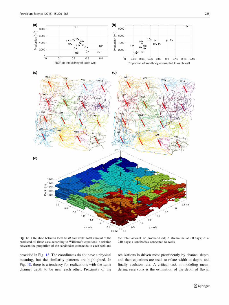
Geobody connectivity metrics, described and discussed

in Renard and Allard (2013), are helpful in assessing

reservoir quality. The connectedness of sands to the wells

is defined based on the minimum time-of-flight from each

block to wells. The minimum time-of-flight (Datta-Gupta

and King 1995) from each well to each block is calculated

using Dijkstra’s algorithm diffusing and updating the time-

of-flight iteratively (Hetland 2014). The travel time through

each block is assumed to be proportional to the inverse of

the permeability (Fig. 17e). Figure 17b indicates that this

metric gives a better approximation. As shown in Fig. 17,

cumulative oil production is not correlated with NGR.

Even though cumulative oil production appears to be

somewhat correlated with sandbody connectedness, this

correlation does not appear to be strong enough to be used

as a reliable estimator. Since sandbodies are more channel-

like rather than sheet-like, their lateral extension impacts

their connectivity to the wells. In fact, this weak correlation

emphasizes the role of preferential paths and connectivity

of sandbodies. As shown in Fig. 17, some sandbodies are

not connected to their closest wells.

3.5 Similarity visualization

As expected, Hmax controls the overall NGR. The similarity

of the realizations is discussed in Sects. 3.3 and 3.4 based

on field- and well-level cumulative production values. The

difference in the ultimate cumulative production values

may also be used to visualize the similarity between the

realizations by projecting them in a metric space using a

multi-dimensional scaling technique. This metric space is

projected to a higher-dimensional space to increase the

models’ separability using a radial basis function kernel.

This technique has been described in detail in Caers

(2011). A 2D projection of realizations in kernel space is

Fig. 16 Relation between overall NGR and total amount of produced oil for reference cases using: a Bridge and Tye’s equation, b Williams’s

equation, c Leeder’s equation, and d all three cases

284 Petroleum Science (2018) 15:270–288

123

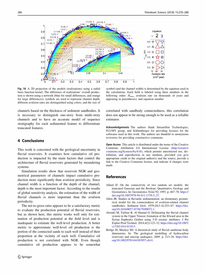
provided in Fig. 18. The coordinates do not have a physical

meaning, but the similarity patterns are highlighted. In

Fig. 18, there is a tendency for realizations with the same

channel depth to be near each other. Proximity of the

realizations is driven most prominently by channel depth,

and then equations are used to relate width to depth, and

finally avulsion rate. A critical task in modeling mean-

dering reservoirs is the estimation of the depth of fluvial

Fig. 17 a Relation between local NGR and wells’ total amount of the

produced oil (base case according to Williams’s equation); b relation

between the proportion of the sandbodies connected to each well and

the total amount of produced oil; c streamline at 60 days; d at

240 days; e sandbodies connected to wells

Petroleum Science (2018) 15:270–288 285

123

channels based on the thickness of sediment sandbodies. It

is necessary to distinguish one-story from multi-story

channels and to have an accurate model of sequence

stratigraphy for each sedimented feature to differentiate

truncated features.

4 Conclusions

This work is concerned with the geological uncertainty in

fluvial reservoirs. It examines how cumulative oil pro-

duction is impacted by the main factors that control the

architecture of fluvial reservoirs generated by meandering

systems.

Simulation results show that reservoir NGR and geo-

metrical parameters of channels impact cumulative pro-

duction more significantly than avulsion periodicity. Since

channel width is a function of the depth of the channel,

depth is the most important factor. According to the results

of global sensitivity analysis, the estimation of the width of

fluvial channels is more important than the avulsion

periodicity.

The net-to-gross ratio appears to be a satisfactory metric

to evaluate the production potential of fluvial reservoirs,

but as shown here, this metric works well only for esti-

mation of production potential at the field level and is

inadequate to estimate the well-level production. A better

metric to approximate well-level oil production is the

portion of the connected sands to each well instead of their

proportion at the vicinity of each well. Cumulative oil

production is not correlated with NGR. Even though

cumulative oil production appears to be somewhat

correlated with sandbody connectedness, this correlation

does not appear to be strong enough to be used as a reliable

estimator.

Acknowledgements The authors thank StreamSim Technologies,

FLUMY group, and Schlumberger for providing licenses for the

softwares used in this work. The authors are thankful to anonymous

reviewers for providing constructive comments.

Open Access This article is distributed under the terms of the Creative

Commons Attribution 4.0 International License (http://creative

commons.org/licenses/by/4.0/), which permits unrestricted use, dis-

tribution, and reproduction in any medium, provided you give

appropriate credit to the original author(s) and the source, provide a

link to the Creative Commons license, and indicate if changes were

made.

References

Allard D. On the connectivity of two random set models: the

truncated Gaussian and the Boolean. Quantitative Geology and

Geostatistics. In: Geostatistics Troia’92; 1993. p. 467–78. https://

doi.org/10.1007/978-94-011-1739-5_37.

Allen JR. Studies in fluviatile sedimentation: an elementary geomet-

rical model for the connectedness of avulsion-related channel

sandbodies. Sediment Geol. 1979;24(3–4):253–67. https://doi.

org/10.1016/0037-0738(79)90072-1.

Alsouki M, Taifour R, Al Hamad O. Delineating the fluvial channel

system in the Upper Triassic formation of the Elward area in the

Syrian Euphrates Graben using 3-D seismic attributes. J Pet

Explor Prod Technol. 2014;4(2):123–32. https://doi.org/10.1007/

s13202-014-0110-5.

Bridge JS, Mackey SD. A theoretical study of fluvial sandstone body

dimensions. In: The geological modelling of hydrocarbon

reservoirs and outcrop analogues; 2009. p. 213–36. https://doi.

org/10.1002/9781444303957.ch14.

Fig. 18 A 2D projection of the models (realizations) using a radial

basis function kernel. The difference of realizations’ overall produc-

tion is shown using a network (blue for small differences, and orange

for large differences); symbols are used to represent channel depth;

different avulsion rates are distinguished using colors; and the size of

symbol (and the channel width) is determined by the equation used in

the calculations. Each field is labeled using three numbers in the

following order: Hmax, avulsion rate (in thousands of years and

appearing in parentheses), and equation number

286 Petroleum Science (2018) 15:270–288

123

Bridge JS, Tye RS. Interpreting the dimensions of ancient fluvial

channel bars, channels, and channel belts from wireline-logs and

cores. AAPG Bull. 2000. https://doi.org/10.1306/a9673c84-

1738-11d7-8645000102c1865d.

Bryant M, Falk P, Paola C. Experimental study of avulsion frequency

and rate of deposition. Geol. 1995;23(4):365–8. https://doi.org/

10.1130/0091-7613(1995)023%3C0365:ESOAFA%3E2.3.CO;2.

Byrnes AP. Reservoir characteristics of low-permeability sandstones

in the Rocky Mountains. Mt Geol. 1997;34:39–48.

Caers J. Modeling uncertainty in the earth sciences. Hoboken: Wiley;

2011.

Caumon G, Journel AG. Early uncertainty assessment: application to

a hydrocarbon reservoir appraisal. In: Leuangthong O, Deutsch

CV, editors. Geostatistics Banff 2004. Springer: Dordrecht;

2005. p. 551–7. https://doi.org/10.1007/978-1-4020-3610-1_56.

Cojan I, Fouche O, Lopez S, Rivoirard J. Process-based reservoir

modelling in the example of meandering channel. In: Leuangth-

ong O, Deutsch CV, editors. Geostatistics Banff 2004. Dor-

drecht: Springer; 2005. p. 611–9. https://doi.org/10.1007/978-1-

4020-3610-1_62.

Collinson JD. Vertical sequence and sandbody shape in alluvial

sequences. In: Miall AD, editor. Fluvial sedimentology—AAPG

Memoir 5; 1977. p. 577–86.

Comunian A, Jha SK, Giambastiani BM, Mariethoz G, Kelly BF.

Training images from process-imitating methods. Math Geosci.

2014;46(2):241–60. https://doi.org/10.1007/s11004-013-9505-y.

Datta-Gupta A, King MJ. A semianalytic approach to tracer flow

modeling in heterogeneous permeable media. Adv Water

Resour. 1995;18(1):9–24. https://doi.org/10.1016/0309-

1708(94)00021-V.

Deviese ES. Modeling fluvial reservoir architecture using Flumy

process. Doctoral dissertation, TU Delft, Delft University of

Technology; 2010.

Fielding CR, Crane RC. An application of statistical modelling to the

prediction of hydrocarbon recovery factors in fluvial reservoir

sequences. In: Ethridge FG, Flores RM, Harvey MD, editors.

Recent developments in fluvial sedimentology. Society of

Economic Paleontologists and Mineralogists, Special Publica-

tions; 1987. p. 321–7. https://doi.org/10.2110/pec.87.39.0321.

Gibling MR. Width and thickness of fluvial channel bodies and valley

fills in the geological record: a literature compilation and

classification. J Sediment Res. 2006;76(5):731–70. https://doi.

org/10.2110/jsr.2006.060.

Hajek EA, Wolinsky MA. Simplified process modeling of river

avulsion and alluvial architecture: connecting models and field

data. Sediment Geol. 2012;257:1–30. https://doi.org/10.1016/j.

sedgeo.2011.09.005.

Hastings JO Jr. Coarse-grained meander-belt reservoirs, Rocky Ridge

field, North Dakota. In: Barwis JH, editor. Sandstone petroleum

reservoirs. Springer: New York; 1990. p. 57–84. https://doi.org/

10.1007/978-1-4613-8988-0_4.

Hetland ML. Python Algorithms: mastering basic algorithms in the

Python Language. New York: Apress; 2014.

Jensen JL. Use of the geometric average for effective permeability

estimation. Math Geol. 1991;23(6):833–40. https://doi.org/10.

1007/bf02068778.

Jones LS, Schumm SA. Causes of avulsion: an overview. In: Smith

ND, Rogers J, editors. Fluvial sedimentology VI. Oxford:

Blackwell Publishing Ltd.; 2009. p. 169–78. https://doi.org/10.

1002/9781444304213.ch13.

Karssenberg D, Tornqvist TE, Bridge JS. Conditioning a process-

based model of sedimentary architecture to well data. J Sediment

Res. 2001;71(6):868–79. https://doi.org/10.1306/051501710868.

Koneshloo M, Aryana SA, Grana D, Pierre JW. A workflow for static

reservoir modeling guided by seismic data in a fluvial system.

Math Geosci. 2017;49(8):995–1020. https://doi.org/10.1007/

s11004-017-9696-8.

Larue DK, Hovadik J. Why is reservoir architecture an insignificant

uncertainty in many appraisal and development studies of clastic

channelized reservoirs? J Pet Geol. 2008;31(4):337–66.

Lauer JW, Parker G. Modeling framework for sediment deposition,

storage, and evacuation in the floodplain of a meandering river:

theory. Water Resour Res. 2008;44:W04425. https://doi.org/10.

1029/2006WR005528.

Leeder MR. Fluviatile fining-upwards cycles and the magnitude of

paleo-channels. Geol Mag. 1973;110(03):265–76.

Lopez S, Cojan I, Rivoirard J, Galli A. Process-based stochastic

modelling: meandering channelized reservoirs. In: de Boer P,

Postma G, van der Zwan K, Burgess P, Kukla P, editors.

Analogue and numerical modelling of sedimentary systems:

from understanding to prediction. Wiley-Blackwell: Special

Publ. 40 of the IAS; 2009. p. 139–44. https://doi.org/10.1002/

9781444303131.ch5.

Lorenz JC, Heinze DM, Clark JA, Searls CA. Determination of

widths of meander-belt sandstone reservoirs from vertical

downhole data, Mesaverde Group, Piceance Creek basin,

Colorado. AAPG Bull. 1985;69(5):710–21. https://doi.org/10.

1306/ad4627ef-16f7-11d7-8645000102c1865d.

Mao S, Journel AG. Generation of a reference petrophysical/seismic

data set: the Stanford V reservoir. Stanford: Stanford Center for

Reservoir Forecasting Report; 1999.

Massonnat GJ. Can we sample the complete geological uncertainty

space in reservoir-modeling uncertainty estimates? SPE J.

2000;5(01):46–59. https://doi.org/10.2118/59801-pa.

Miall AD. Fluvial depositional systems. New York: Springer; 2014.

Nojabaei B, Siripatrachai N, Johns RT, Ertekin T. Effect of saturation

dependent capillary pressure on production in tight rocks and

shales: a compositionally-extended black oil formulation. In:

SPE Eastern Regional Meeting, Charleston, WV, USA; 2014.

https://doi.org/10.2118/171028-ms.

Pizzuto JE, Moody JA, Meade RH. Anatomy and dynamics of a

floodplain, Powder River, Montana, USA. J Sediment Res.

2008;78(1):16–28. https://doi.org/10.2110/jsr.2008.005.

Pranter MJ, Sommer NK. Static connectivity of fluvial sandstones in a

lower coastal-plain setting: an example from the Upper Creta-

ceous lower Williams Fork Formation, Piceance Basin, Color-

ado. AAPG Bull. 2011;95(6):899–923. https://doi.org/10.1306/

12091010008.

Pyrcz MJ, Deutsch CV. Geostatistical reservoir modeling. Oxford:

Oxford University Press; 2014.

Ramon JC, Cross T. Characterization and prediction of reservoir

architecture and petrophysical properties in fluvial channel

sandstones, middle Magdalena Basin, Colombia. CT&F-Ciencia

Tecnologıa y Futuro. 1997;1(3):19–46. https://doi.org/10.1306/

1d9bbf5d-172d-11d7-8645000102c1865d.

Ren G, Rafiee J, Aryana SA, Younis RM. A Bayesian model selection

analysis of equilibrium and nonequilibrium models for multi-

phase flow in porous media. Int J Multiph Flow.

2017;89:313–20. https://doi.org/10.1016/j.ijmultiphaseflow.

2016.11.006.

Renard P, Allard D. Connectivity metrics for subsurface flow and

transport. Adv Water Resour. 2013;51:168–96. https://doi.org/

10.1016/j.advwatres.2011.12.001.

Rezaee H, Mariethoz G, Koneshloo M, Asghari O. Multiple-point

geostatistical simulation using the bunch-pasting direct sampling

method. Comput Geosci. 2013;54:293–308. https://doi.org/10.

1016/j.cageo.2013.01.020.

Slatt RM. Stratigraphic reservoir characterization for petroleum

geologists, geophysicists, and engineers. Amsterdam: Elsevier;

2006. https://doi.org/10.1016/s1567-8032(06)x8035-7.

Petroleum Science (2018) 15:270–288 287

123

Slingerland R, Smith ND. River avulsions and their deposits. Annu

Rev Earth Planet Sci. 2004;32:257–85. https://doi.org/10.1146/

annurev.earth.32.101802.120201.

Strebelle S. Conditional simulation of complex geological structures

using multiple-point statistics. Math Geol. 2002;34(1):1–21.

https://doi.org/10.1007/s11004-013-9510-1.

Thiele MR, Batycky RP, Blunt MJ. A streamline-based 3d field-scale

compositional reservoir simulator. In: SPE Annual Technical

Conference and Exhibition 1997 Jan 1. Society of Petroleum

Engineers; 1997. https://doi.org/10.2523/38889-ms.

Tye RS. Quantitatively modeling alluvial strata for reservoir devel-

opment with examples from Krasnoleninskoye Field, Russia.

J Coast Res. 2013;69(sp1):129–52. https://doi.org/10.2112/si_

69_10.

Utts JM, Heckard RF. Mind on statistics. Boston: Cengage Learning;

2011.

Williams GP. River meanders and channel size. J Hydrol.

1986;88(1–2):147–64. https://doi.org/10.1016/0022-

1694(86)90202-7.

Zhang T, Zhang X, Lin C, Yu J, Zhang S. Seismic sedimentology

interpretation method of meandering fluvial reservoir: from

model to real data. J Earth Sci. 2015;26(4):598–606. https://doi.

org/10.1007/s12583-015-0572-5.

Zhang Y, Song C, Zheng S, Yang DT. Simultaneous estimation of

relative permeability and capillary pressure for tight formations

from displacement experiments. In: SPE Canadian Unconven-

tional Resources Conference 2012 Jan 1. Society of Petroleum

Engineers; 2012. https://doi.org/10.2118/162663-ms.

288 Petroleum Science (2018) 15:270–288

123