Uncertainty in geological and hydrogeological data - hessd

HESSD3, 2675–2706, 2006

Uncertainty ingeological and

hydrogeological data

B. Nilsson et al.

Title Page

Abstract Introduction

Conclusions References

Tables Figures

J I

J I

Back Close

Full Screen / Esc

Printer-friendly Version

Interactive Discussion

EGU

Hydrol. Earth Syst. Sci. Discuss., 3, 2675–2706, 2006www.hydrol-earth-syst-sci-discuss.net/3/2675/2006/© Author(s) 2006. This work is licensedunder a Creative Commons License.

Hydrology andEarth System

SciencesDiscussions

Papers published in Hydrology and Earth System Sciences Discussions are underopen-access review for the journal Hydrology and Earth System Sciences

Uncertainty in geological andhydrogeological dataB. Nilsson, A. L. Højberg, J. C. Refsgaard, and L. Troldborg

Geological Survey of Denmark and Greenland, Copenhagen, Denmark

Received: 26 April 2006 – Accepted: 17 August 2006 – Published: 31 August 2006

Correspondence to: B. Nilsson ([email protected])

2675

http://www.hydrol-earth-syst-sci-discuss.net

http://www.hydrol-earth-syst-sci-discuss.net/3/2675/2006/hessd-3-2675-2006-print.pdf

http://www.hydrol-earth-syst-sci-discuss.net/3/2675/2006/hessd-3-2675-2006-discussion.html

http://www.copernicus.org/EGU/EGU.html

HESSD3, 2675–2706, 2006



B. Nilsson et al.

Title Page



Tables Figures

J I

J I

Back Close

Full Screen / Esc



EGU

Abstract

Uncertainty in conceptual model structure and in environmental data is of essential in-terest when dealing with uncertainty in water resources management. To make quan-tification of uncertainty possible it is necessary to identify and characterise the uncer-tainty in geological and hydrogeological data. This paper discusses a range of available5

techniques to describe the uncertainty related to geological model structure and scaleof support. Literature examples on uncertainty in hydrogeological variables such assaturated hydraulic conductivity, specific yield, specific storage, effective porosity anddispersivity are given. Field data usually have a spatial and temporal scale of supportthat is different from the one on which numerical models for water resources man-10

agement operate. Uncertainty in hydrogeological data variables is characterised andassessed within the methodological framework of the HarmoniRiB classification.

1 Introduction

Uncertainty of geological and hydrogeological features is of great interest when dealingwith uncertainty in relation to the Water Framework Directive (WFD). One of the key15

sources of uncertainty of importance for evaluating the effect and cost of a measurein relation to preparing a WFD-compliant river basin management plan is to assessuncertainty on model structure, input data and parameter variables in relation to hydro-logical models. Uncertainty in hydrogeological variables is typically done by the use ofnumerical models.20

Neuman and Wierenga (2003) summarise where uncertainties in model results orig-inate from in addition to parameter uncertainty. Uncertainties arise firstly from incom-plete definitions of the final conceptual framework that determines model structure;secondly from spatial and temporal variations in hydrological variables that are eithernot fully captured by the available data or not fully resolved by the model; and finally25

from the scaling behaviour of the hydrogeological variables. Whereas much has been

2676





HESSD3, 2675–2706, 2006



B. Nilsson et al.

Title Page



Tables Figures

J I

J I

Back Close

Full Screen / Esc



EGU

written about the mathematical component of hydrogeological models, relatively littleattention has been devoted to the conceptual component. In most mathematical mod-els of subsurface flow and transport, the conceptual framework is assumed to be given,accurate and unique (Dagan et al., 2003).

It has been recognised for long that the structural uncertainty often can be the domi-5

nating factor (Carrera and Neuman, 1986; Harrar et al., 2003; Troldborg, 2004; Højbergand Refsgaard, 2005; Poeter and Anderson, 2005; Eaton, 2006). This is especially im-portant in groundwater modelling, where the geological structure is dominant for thegroundwater flow but where specific knowledge of the geology at the same time is verylimited. Simulating flow through heterogeneous geological media requires that the nu-10

merical models capture the important aspects of the flow domain structures. Only avery sparse selection of operational methods has been developed to quantify structuraluncertainties in geological models.

In the international literature significant attention has been given to estimation ofparameter uncertainties on the variability in parameter values which can vary many15

decades and therefore cannot be directly measured but are often derived from modelcalibration (e.g. Samper et al, 1990; Poeter and Hill, 1997; Cooley, 2004). Scalingbehaviour of hydrogeological variables is another challenge within the hydrological sci-ence. This paper deals with assessing the uncertainty in geological and hydrogeologi-cal data.20

The overall aim of this paper is to illustrate how currently available techniques and re-sults can be used to describe the uncertainty related to geological and hydrogeologicaldata at the river basin scale. Specific objectives are firstly to characterize uncertaintywithin the methodological framework given by Brown et al. (2005) and van Loon etal. (2006)1. Secondly, to give examples on variability from literature on input data, pa-25

rameter values and geological model structure interpretations. This paper will havemain focus on physical data uncertainty in the saturated zone unlike van der Keur et

1van Loon, E., Brown, J., and Heuvelink, G.: A framework to describe hydrological uncer-tainties, Hydrol. Earth Syst. Sci. Discuss., in preparation, 2006.

2677





HESSD3, 2675–2706, 2006



B. Nilsson et al.

Title Page



Tables Figures

J I

J I

Back Close

Full Screen / Esc



EGU

al. (2006), that primarily covers the physical and chemical data in the unsaturated zone.The present work in this paper is part of an ongoing research project, HarmoniRiB,

that is supported under EU 5th Framework Programme. The overall goal of Har-moniRiB is to develop methodologies for quantifying uncertainty and its propagationfrom raw data to concise management information. Refsgaard et al. (2005) present5

further details about the HarmoniRiB project.

2 Uncertainty in geological model structure

2.1 What is a hydrogeological conceptual model?

Many scientists and practitioners have difficulties finding consensus on defining termi-nology and guiding principles on hydrogeological conceptual modelling. Neuman and10

Wierenga (2003) describe a hydrogeological model as a framework that serves to anal-yse, qualitatively and quantitatively, subsurface flow and transport at a site in a way thatis useful for review and performance evaluation.

Anderson and Woessner (1992) point out that a conceptual model is a simplificationof the problem, where the associated field data are organised in such a way, that the15

system can be analysed more readily. When numerical modelling is considered theconceptual model should define the hydrogeological structures relevant to be includedin the numerical model given the modelling objectives and requirements, and helpto keep the modeller tied into reality and exert a positive influence on his subjectivemodelling decisions. The nature of the conceptual model determines the dimensions20

of the model and the design of the grid.An important part of the conceptual model for groundwater modelling is related to the

geological structure and how this is represented in the numerical model. Among hydro-geologists it is very common to use the hydrofacies modelling approach to constructconceptual models for specific types of sedimentary environments. Hydrofacies or25

hydrogeological facies are used for homogeneous but not necessarily isotropic hydro-

2678





HESSD3, 2675–2706, 2006



B. Nilsson et al.

Title Page



Tables Figures

J I

J I

Back Close

Full Screen / Esc



EGU

geological units that are formed under conditions, which lead to similar characteristichydraulic properties (Anderson, 1989). Numerous papers address the hydrogeologicalconceptualisation using hydrofacies: E.g. in glacial melt water-stream sediment and till(Anderson, 1989), buried valley aquifers (Ritzi et al., 2000); and alluvial fan depositionalsystems (Weissmann and Fogg, 1999). Comprehensive reviews and compilations of5

this issue can be found in e.g. Koltermann and Gorelick (1996) and Fraser and Davis(1998).

2.2 Where do uncertainties arise from in conceptual models ?

Descriptive methods are used to create images of subsurface geological depositionalarchitecture by combining site-specific and regional data with conceptual depositional10

models and geological insight. For a given field site, descriptive methods produce onedeterministic image of the aquifer architecture, acknowledging heterogeneity but notdescribe it in a deterministic way at scales ranging from stratigraphical features (mscale) to basin fill (river basin scale). Large scale heterogeneity may be recognisedbut most often smaller scale heterogeneity is not captured. Often, sedimentary strata15

are divided into multiple layers designated as aquifers or aquitards. The assumptionis made that geological facies define the spatial arrangement of hydraulic propertiesdominating groundwater flow and transport behaviour (Anderson, 1989; Fogg, 1986;Klingbeil et al., 1999; Bersezio et al., 1999; Willis and White, 2000). This assumptioncan be checked using hydraulic property measurements to define facies.20

2.3 Strategies on assessing uncertainty in the geological model structure

Errors in the conceptual model structure may be analysed by considering differentconceptualisations or scenarios. In the scenario approach a number of alternativeplausible conceptual models are formulated and applied in a model to provide modelpredictions. The differences between the model predictions based on the alternative25

conceptualisations are then taken as a measure of the model structure uncertainty.

2679





HESSD3, 2675–2706, 2006



B. Nilsson et al.

Title Page



Tables Figures

J I

J I

Back Close

Full Screen / Esc



EGU

The influence of different model conceptualisations may be evaluated by having al-ternative conceptual models based on different geological interpretations (Selroos etal., 2001; National Research Council, 2001). Harrar et al. (2003) and Højberg andRefsgaard (2005) present two different examples, both using three different conceptualmodels, based on three alternative geological interpretations for multi-aquifer system5

representative of eastern part of Denmark with glacial till plains (Højberg and Refs-gaard, 2005) and in sandy outwash plains in the western part of Denmark (Harrar etal., 2003). Each of the models was calibrated against piezometrical head data usinginverse optimisation. In both studies, the three models performed equally well in re-producing the groundwater head used for calibration. Using the models in predictive10

mode they resulted in very similar well field capture zones. However, when the modelswere used to extrapolate beyond the calibration data for predictions of solute transportand travel times the three models differed dramatically. When assessing the uncer-tainty contributed by the model parameter values using Monte Carlo simulations, theoverlap of uncertainty ranges between the three models by Højberg and Refsgaard15

(2005) significantly decreased when moving from groundwater heads to capture zonesand travel times. The larger the degree of extrapolation, the more the underlying con-ceptual model dominates over the parameter uncertainty and the effect of calibration.However, the parameter uncertainty can not compensate for the variability (uncertainty)in the geological model structure.20

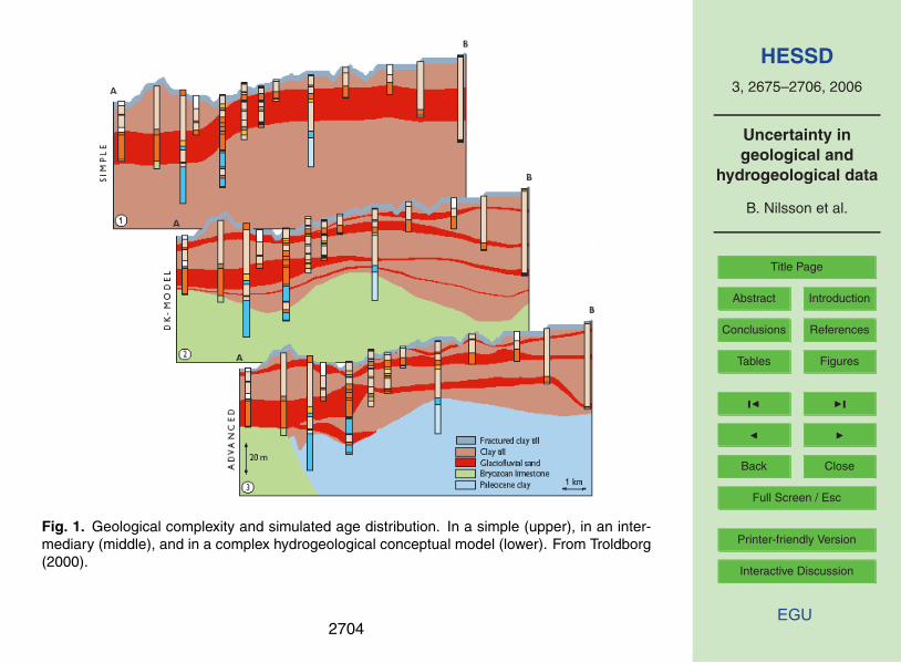
The importance of geological interpretations on groundwater flow and age (particletracking) predictions have been studied by Troldborg (2000, 2004). Using a zonationapproach three different conceptual models were constructed based on an extensiveborehole database (Fig. 1). The three models differed in complexity. Calibrations of themodels were performed using inverse calibration against hydraulic head and discharge25

measurements. Numerical simulation of groundwater age was carried out using aparticle tracking model. Although the three models provided very similar calibrationfits to groundwater heads, a model extrapolation to predictions of groundwater agesrevealed very significant differences between the three models, which were explained

2680





HESSD3, 2675–2706, 2006



B. Nilsson et al.

Title Page



Tables Figures

J I

J I

Back Close

Full Screen / Esc



EGU

by the differences in underlying hydrogeological interpretations.Conditional geostatistical simulations is frequently used to address issues related to

spatial distribution of conductivity (de Marsily et al., 1998; Kupfersberger and Deutsch,1999). Most frequently, though, it is used after conceptualization of aquifer structuresto generate conditional realizations of conductivity within hydrological units (facies)5

e.g. input for Monte Carlo analysis. A good example of this is found in Zimmermanet al. (1998), where they compared seven different geostatistical approaches in combi-nation with inverse modelling to simulate travel times and travel paths of conservativetracer through four synthetic aquifer data sets.

Geostatistical methods that can simulate hydrofacies distributions at different scale10

are divided into structural and process imitating methods (Koltermann and Gorelick,1996). De Marsily et al. (1998) point out that process imitating methods cannot beconditioned to local available information. Carle and Fogg (1996, 1997) present atransition probability geostatistical framework that can be conditioned to hard as wellas soft data in simulating hydrofacies distributions. There are several examples on15

application which include simulation of alluvial fan systems (Fogg et al., 1998; Weiss-mann et al., 1999; Weissmann and Fogg, 1999), river valley aquifer systems (Ritzi etal., 1994, 2000), Quaternary aquifer complex (Troldborg et al., 20062) and sandlensesdistribution within glacial till in (Sminchak et al., 1996; Petersen et al., 2004).

Neuman and Wieranga (2002) present a generic strategy that embodies a system-20

atically and comprehensive multiple conceptual model approach, including hydrogeo-logical conceptualisation, model development and predictive uncertainty analysis. Thestrategy encourages an iterative approach to modelling, whereby an initial conceptual-mathematical model is gradually altered and/or refined until one or more like alterna-tives have been identified and analysed.25

Professionals within the discipline have not yet agreed upon a procedure for rank-

2Troldborg, L., Refsgaard, J. C., Jensen, K. H., Engesgaard, P., and Carle, S. F.: Applicationof transition probability geostatistics in hydrological modeling of a Quaternary aquifer complex,in preparation, 2006.

2681





HESSD3, 2675–2706, 2006



B. Nilsson et al.

Title Page



Tables Figures

J I

J I

Back Close

Full Screen / Esc



EGU

ing or weighting conceptual models. Poeter and Anderson (2005) introduce a mul-timodel ranking and interference, which is a simple and effective approach for theselection of a best model: one that balances under fitting with over fitting. Neumanand Wierenga (2003) propose and apply the Maximum Likelihood Bayesian Averaging(MLBA) approach for assessment of the joint predictive uncertainties in the conceptual-5

mathematical model structure and its parameters. Finally, Refsgaard et al. (2006) pro-pose a strategy that combines multiple conceptual models and the pedigree approach(Funtowicz and Ravetz, 1990) for assessing the overall tenability of models in one for-malised protocol. The level of subjectivity can to some degree be reduced using expertelicitation, which is a structured process to elicit subjective judgements from experts.10

3 Scaling issues

One of the great and very general challenges within the hydrological science is to un-derstand the impact of changing scales on various process descriptions and parametervalues. The average volume of hydrogeological measurements (also named supportvolume) is ranging many orders of magnitude depending on the size of volume repre-15

senting the individual measurements. Spatial heterogeneity as a function of scale iswell documented in the literature for saturated hydraulic conductivity (Clauser, 1992;Sanchez-Vila et al., 1996; Nilsson et al., 2001). Values of the saturated hydraulicconductivity depend on the volume of substrate sampled by the applied hydraulic test-ing method. A literature example in coarse-grained fluvial sediments (Bradbury and20

Muldoon, 1990) is shown in Fig. 2. It is evident that the mean hydraulic conductivityincreases as the support volume of the tests increases.

3.1 Classification of scales of heterogeneity

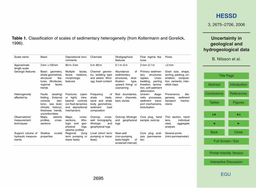
Aquifers contain many scales of hydrofacies or hydrogeological facies, which controlsthe hydraulic conductivity structure. The descriptive nature of many classifications25

2682





HESSD3, 2675–2706, 2006



B. Nilsson et al.

Title Page



Tables Figures

J I

J I

Back Close

Full Screen / Esc



EGU

makes them somewhat subjective; however, they provide a useful basis for compar-ison between multiple scales of geological heterogeneity (Koltermann and Gorelick,1996) (Table 1). Scales of geological and hydraulic conductivity structure are based on(a) size of the geological features, (b) genetic origin, (c) support length (porous mediameasurement volumes).5

3.2 Support volume of hydrogeological measurements

Subsurface investigations like pumping tests or tracer tests are only able to provideeffective parameters at a scale much larger than the typical length of structures ina heterogeneous aquifer (Klingbeil et al., 1999). Results from many different hydro-geological field studies, for example Borden (Sudicky, 1985) and Cape Cod (Hess,10

1990; Hess et al., 1991) show that the resolution of data acquisition necessary forpredicting transport parameters cannot be achieved by standard subsurface investi-gation techniques such as pumping tests, tracer tests, flowmeter measurements andcore analysis. Although flowmeter measurements and core analysis data give enoughdetails to characterise heterogeneous hydraulic conductivity and porosity distributions15

in the vertical direction, the boreholes often have spacings that are too large for infer-ring heterogeneous parameters in the horizontal direction. Thus the lateral continuityof subsurface structures is often not known. Based on this experience more detailedinformation is needed, particularly on the small-scale horizontal structure and conse-quently the distribution of parameters in aquifers (Anderson, 1989). Generally, real20

aquifers are not accessible for investigation to directly measure hydrogeological pa-rameters. An outcrop composed of a similar stratigraphy and of similar lithologies asthe aquifer may be viewed as an analogue of the aquifer (“aquifer/ outcrop analogue”)representing an accessible formation for the examination of spatial geometries and forin-situ measurements of hydrogeological parameters at the smaller scale.25

2683





HESSD3, 2675–2706, 2006



B. Nilsson et al.

Title Page



Tables Figures

J I

J I

Back Close

Full Screen / Esc



EGU

3.3 Examples dealing with scaling

Frykman and Deutsch (2002) demonstrate a practical application of the volume-variance relations in oil reservoir characterisation in the Danish North Sea for upscalingand downscaling methods to integrate data of different scales. The volume-variancescaling laws were used on traditional core and well logs representing fine-scale ge-5

ological heterogeneities to seismic or well test data capturing much larger scales. Agood understanding of the support volume for the different scales is necessary and theup- and downscaling effects must be considered.

An example of upscaling of uncertainty on groundwater heads from a point scale toa 1 km2 grid scale is given in Henriksen et al. (2003). Groundwater head data are mea-10

sured in observation wells, i.e. with a measurement support scale of a few cm2. Whenused to compare with simulated heads simulated by a groundwater model with a spatialresolution of 1 km2 the relevant uncertainty of the measured head should also includeits uncertainty in representing average groundwater head over the 1 km2. In additionthe point scale value representing a small time scale (e.g. 10 s) should be upscaled to15

show its representativeness of an average annual value, taking the seasonal variationsinto account. The sources of uncertainty and their respective contributions in this re-spect are shown in Table 2. Assuming mutual independence between these individualerrors the aggregated uncertainty of the observed head data relative to model simula-tions at a 1 km scale can be estimated as the square root of the sum of the squared20

errors, summing up to 3.1 m.

4 Uncertainty in hydrogeological data

4.1 Variability on hydraulic properties

Data on spatial variability investigated by means of geostatistical methods have ob-tained significant attention in the scientific literature (Isaaks and Srivastava, 1989). For25

2684





HESSD3, 2675–2706, 2006



B. Nilsson et al.

Title Page



Tables Figures

J I

J I

Back Close

Full Screen / Esc



EGU

all practical purposes at the time scales relevant for this paper the variables are consid-ered invariant. Several studies have focused on the determination of spatial correlationlength scales for different hydraulic properties (e.g. Dagan, 1986; Gelhar, 1993). Vari-ability becomes uncertain because it cannot be captured by direct field or laboratorymeasurements. Instead, the parameter variability is recognised by the geostatistical5

measure like mean, variance and correlation length.

4.1.1 Hydraulic conductivity (K)

Gelhar (1993) summarise the standard deviation and correlation lengths (λ) of hy-draulic conductivity from several field studies in Table 3, which covers a wide rangeof field scales and seems to indicate that the length scale of field data for which cor-10

relation length and standard deviation have been assessed increases with increasingfield scale.

Different measurement techniques used to determine saturated hydraulic conductiv-ity representing 13 orders of magnitude in a coarse-grained fluvial material are shownin Fig. 2. The hydraulic conductivity of various geological materials is ranging multiple15

orders of magnitude with unfractured bedrocks and matrix permeability in glacial tills inthe lower end and unconsolidated sediments in the middle to upper end.

4.1.2 Storage coefficients, effective porosity and dispersivity

Correlation lengths of specific yield (Sy ), specific storage (Ss) and effective porosity (n)are not found in the literature. The range of values related to different soil types are20

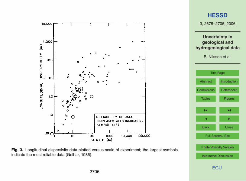
available (Table 4). The longitudinal dispersivity (α) has been compiled in Fig. 3 frommany field sites with very different geological setting around the world (Gelhar, 1986).These data indicates that a longitudinal dispersivity in the range of 1 to 10 m would bereasonable for a site of dimensions on the order of 1 km, whereas the range of 10 to1000 m would cover the river basin length scale on the order of few km to more than25

100 km. The dispersivity value typically varies by 2 to 3 orders of magnitude depending

2685





HESSD3, 2675–2706, 2006



B. Nilsson et al.

Title Page



Tables Figures

J I

J I

Back Close

Full Screen / Esc



EGU

on which length that are of interest.

4.2 Classification of data uncertainty in accordance to HarmoniRiB terminology andclasses

As part of the data processing the HarmoniRiB project partners have characterisedand assessed the data uncertainty using the new methodology described by Brown5

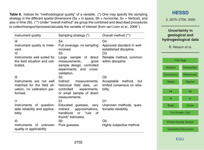
et al. (2005) and using the DUE (Data Uncertainty Engine) software tool (Brown andHeuvelink, 2006). This new methodology has been further elaborated in van Loon etal. (2006)1. Tables 5–8 show the key characteristics used to characterise data uncer-tainty. The terms in these tables are used in characterising the key characteristics ofdata uncertainty in the hydrogeological variables.10

4.2.1 Attribute, empirical and longevity uncertainty

The specific yield, effective porosity and dispersivity are all assessed to typically havea measurement space support of about 100 cm3. Hydraulic conductivity and specificstorage have a measurement space support scale ranging from 10−5 to 109 m3 de-pending on sample size of the applied method to determine the variable. The uncer-15

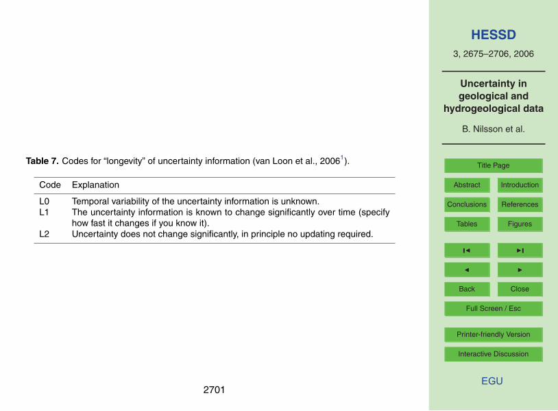
tainty category is for all variables classified as C1 (cf. Table 5), which means all vari-ables are assumed to vary in space but not in time. The type of empirical uncertainty isclassified as M1 (Table 6) for all five parameters implying that uncertainty can be char-acterised statistically by use of probability density functions. The relative age (denotedby the term “longevity”) of uncertainty description is classified as L2 (Table 7) for all20

variables, which means the uncertainty does not change significantly so no updating isrequired.

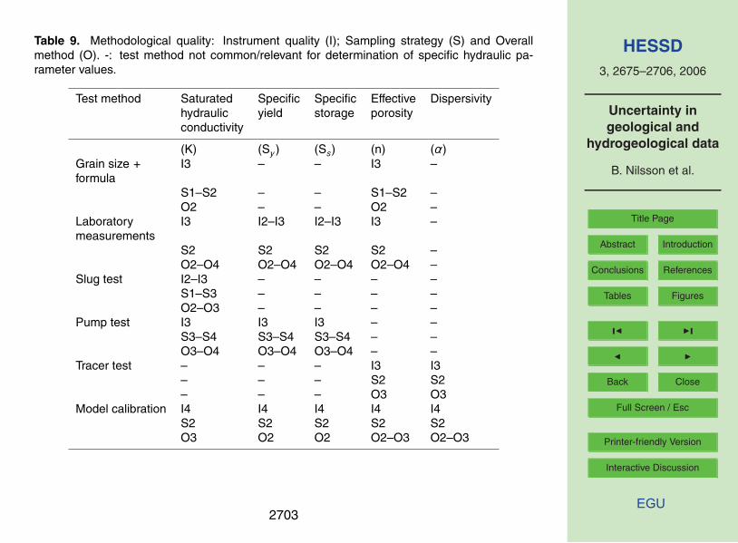
4.2.2 Methodological quality uncertainty

Saturated hydraulic conductivity (K): The K values can be determined by all test meth-ods represented in Table 9 from point scale (laboratory measurements) to model cal-25

2686





HESSD3, 2675–2706, 2006



B. Nilsson et al.

Title Page



Tables Figures

J I

J I

Back Close

Full Screen / Esc



EGU

ibration scale (typical grid size of 1 km2). However tracer tests are rarely used fordetermination of K values, why the methodological quality have been found irrelevantfor evaluation. The instrument quality is classified as I3 (instruments well suited for thefield situation and calibrated) except the model calibration scale, where the evaluationof instrument quality is not relevant. The sampling strategy is showing increasing in-5

dices (i.e. increasing quality) with increasing support volume, i.e. the small scale mea-surements like grain sieving analysis and other laboratory measurements (e.g. leach-ing columns experiments or intact columns) are typically ranging between S1 to S2indices. Slug test measurements vary even more from S1 to S3 depending on thesite specific geological heterogeneity. Pump tests are giving the best coverage. Re-10

garding the overall method indices are laboratory methods ranging significantly due toscale effects. On the other hand both specific laboratory measurements and pump testare reliable methods and there are even approved standards for measuring saturatedhydraulic conductivity on laboratory and field scale. Model calibrations using inversetechniques (auto-calibration) is also a reliable and commonly used method.15

Specific yield (Sy ): Retention curve determinations on laboratory scale has instru-ment quality range from not well to well match of the field conditions. Keur et al. (2006)describe more thoroughly the application of retention curves to determination of physi-cal parameters on various scales. Pump tests have the highest instrument quality, bestcoverage of sampling strategy and is an overall reliable method. Model calibration is20

commonly used and seen as an acceptable method for Sy estimation but there arelimited consensus on the reliability of the results.

Specific storage (Ss) has been characterised with the same indices ranking as Sybut on laboratory scale are retentions curves exchanged with geotechnical triaxial teststo determine specific storage.25

Effective porosity (n): This variable has the instrument quality well suited at bothsmall and large scale. All test methods are ranking between educated guesses toindirect measurements. Results derived from tracer tests can among others be used foreffective porosity estimation. All test methods are grouped as acceptable methods even

2687





HESSD3, 2675–2706, 2006



B. Nilsson et al.

Title Page



Tables Figures

J I

J I

Back Close

Full Screen / Esc



EGU

with some specific methods appearing as approved standards for porosity measuring.Dispersivity (α): The alpha value is limited to be determined from the larger scale

methods: tracer test and model calibration.In general, the HarmoniRiB framework indices for the methodological quality in-

crease with increasing support volume, which the different test methods represent. In-5

dividual indices show higher variability at small scale test methods compared to largerscale methods due to effects of spatial scale.

5 Discussion and conclusions

Uncertainty assessment is an important aspect of water resources management. Firstof all, water management decisions should be made with full information on the un-10

derlying uncertainties. Secondly, credibility of model predictions among stakeholdersis important for achieving consensus and robust decisions. Overselling of model ca-pabilities is ‘poison’ for establishing such credibility. Instead, explicit information onthe involved uncertainties may help creating a more balanced view on the capability ofmodels and in this way pave the road for improving the credibility of models.15

Assessments of uncertainty in hydrogeological data and conceptual models are pre-requisites for assessment of uncertainty in model predictions, and as such they arecrucial. Uncertainty assessments are common in the scientific community, but not yetin the professional world of water management. We therefore have a major task inpromoting the use of our uncertainty concepts and tools in practise.20

In this paper examples are given from the most current scientific literature that dealswith uncertainty on model structure and uncertainty on parameter variables. Quantifi-cation of the uncertainty due to model structure is an area of novel interest, where onlyfew operational methods have been developed. Some of the present techniques todescribe the uncertainty related to geological model structure are presented and some25

strategies on interpretation of geological model structure are identified. In addition, un-certainty and scale of support in the hydrogeological data variables: saturated hydraulic

2688





HESSD3, 2675–2706, 2006



B. Nilsson et al.

Title Page



Tables Figures

J I

J I

Back Close

Full Screen / Esc



EGU

conductivity, specific yield, specific storage, effective porosity and dispersivity are eval-uated. The variables are related to the following test methods: grain size analysis,other laboratory measurements, slug tests, pump tests, tracer tests and model calibra-tions. Uncertainty in the hydrogeological data variables is in this study characterisedand assessed within the methodological framework of the HarmoniRiB classification,5

where the rating of the quality of methods can be given in a more structured overview.In general, the HarmoniRiB framework indices for the methodological quality increasewith increasing support volume, which the different test methods represent. Individ-ual indices shows higher variability at small scale test methods compared to largerscale methods due to effects of spatial scale. The use of the HarmoniRiB classification10

makes it possible to carry out systematic comparison of uncertainties arising in differ-ent data types required for evaluating the effect and cost of a measure in relation topreparing a water management plan in relation to the Water Framework Directive.

Scientifically there are two major tasks ahead of us to be solved. While the statisticaltools for characterising uncertainty are well developed, it should be realised that many15

aspects of uncertainty cannot be quantified but have to be described qualitatively orsubjectively. This applies particularly to geological uncertainty where knowledge ongeological history and formation processes basically is qualitative. If we do not al-low qualitative descriptions of uncertainty we exclude much of the geological knowl-edge. The second major challenge lies in handling of model structure uncertainty,20

which in case of groundwater models corresponds to uncertainty in hydrogeologicalconceptual models. In cases where models are used for making extrapolatory pre-dictions, i.e. predictions beyond conditions and data for which a model was calibratedand tested, model structure uncertainty is known often to be the dominant source ofuncertainty. And such extrapolations are situations where models are most needed,25

because relevant explicit data on the decisions variables of interest do not exist. Whilemethods for handling uncertainty in geological data are well known we have a majorchallenge in developing and testing concepts for handling model structure uncertainty,and to make best possible use of qualitative geological knowledge in this context.

2689





HESSD3, 2675–2706, 2006



B. Nilsson et al.

Title Page



Tables Figures

J I

J I

Back Close

Full Screen / Esc



EGU

Acknowledgements. The present work was carried out within the Project “Harmonised Tech-niques and Representative River Basin Data for Assessment and Use of Uncertainty Informa-tion in Integrated Water Management (HarmoniRiB)”, which is partly funded by the EC Energy,Environment and Sustainable Development programme (Contract EVK1-CT2002-00109).

References5

Anderson, M. P.: Hydrogeologic facies models to delineate large-scale spatial trends in glacialand glaciofluvial sediments, Geological Society America Bulletin, 101, 501–511, 1989.

Anderson, M. P. and Woessner, W. W.: Applied groundwater modelling, simulation of flow andadvective transport, Academic Press, San Diego, California, 1992.

Bersezio, R., Bini, A., and Giudici, M.: Effects of sedimentary heterogeneity on groundwater10

flow in a Quaternary pro-glacial delta environment: joining facies analysis and numericalmodelling, Sedimentary Geology, 129, 327–344, 1999.

Bradbury, K. R. and Muldoon, M. A.: Hydraulic conductivity determination in lithified glacial andfluvial materials, in: Ground Water and Vadose Zone Monitoring, ASTM STP 1053, editedby: Nielsen, D. M. and Johnsen, A. I., American Society for testing Materials, Philadelphia,15

138–151, 1990.Brown, J. D., Heuvelink, G. B. M., and Refsgaard, J. C.: An integrated framework for assessing

and recording uncertainties about environmental data, Water Sci. Technol., 52(6), 153–160,2005.

Brown, J. D. and Heuvelink, G. B. M.: Data Uncertainty Engine (DUE) User’s Manual, University20

of Amsterdam, http://www.harmonirib.com, 2006.Carrera, J. and Neuman, S. P.: Estimation of aquifers parameters under transient and steady

state conditions: 1. Maximum likelihood method incorporating prior information, Water Re-sour. Res., 22, 199–210, 1986.

Carle, S. F. and Fogg, G. E.: Transition probability based on indicator geostatistics, Mathemat-25

ical Geology, 28, 453–477, 1996.Carle, S. F. and Fogg, G. E.: Modelling spatial variability with one and multidimensional

continuous-lag Markov chains, Mathematical Geology, 29, 891–917, 1997.Clauser, C.: Permeability of crystalline rocks, Eos, 73, 233–238, 1992.

2690





http://www.harmonirib.com

HESSD3, 2675–2706, 2006



B. Nilsson et al.

Title Page



Tables Figures

J I

J I

Back Close

Full Screen / Esc



EGU

Cooley, R. L.: A theory for modelling ground-water flow in heterogeneous media, U.S.G.S.Professional Paper, vol. P 1679, U.S. Geological Survey, Denver, CO, 220 pp., 2004.

Dagan, G.: Statistical theory of groundwater flow and transport: Pore to laboratory, laboratoryto formation and formation to regional scale, Water Resour. Res., 22(9), 120S–134S, 1986.

Dagan, G., Fiori, A., and Jankovic, I.: Flow and transport in highly heterogeneous formations:5

1. Conceptual framework and validity of first-order approximations, Water Resour. Res., 39,1268, doi:10.1029/2002WR001717, 2003.

de Marsily, G., Delay, F., Teles, V., and Schafmeister, M. T.: Some current methods to representthe heterogeneity of natural media in hydrogeology, Hydrogeology Journal, 6(1), 115–130,1998.10

Eaton, T.: On the importance of geological heterogeneity for flow simulation, SedimentaryGeology, 184, 187–201, 2006.

Fogg, G. E.: Groundwater flow and sand body interconnectedness in a thick multiple aquifersystem, Water Resour. Res., 22, 679–694, 1986.

Fogg, G. E., Noyes, C. D., and Carle, S. F.: Geologically based model of heterogeneous hy-15

draulic conductivity in an alluvial setting, Hydrogeology Journal, 6(1), 131–143, 1998.Fraser, G. S. and Davis, J. M. (Eds.): Hydrogeologic models of sedimentary aquifers, SEPM

Concepts in Hydrology and Environmental geology, vol. 1. Society for Sedimentary Geology,Tulsa, OK, 180 pp., 1998.

Freeze, R. A. and Cherry, J. A.: Groundwater, Prentice Hall, Englewood Cliffs, NJ 07632, USA,20

1979.Frykmann, P. and Deutsch, C. V.: Practical application of geostatistical scaling laws for data

integration, Petrophysics, 43(3), 153–177, 2002.Funtowicz, S. O. and Ravetz, J. R.: Uncertainty and Quality in Science for Policy, Kluwer,

Dordrecht, 229 p., 1990.25

Gelhar, L. W.: Stochastic subsurface hydrology from theory to application, Water Resour. Res.,22(9), 135S–145S, 1986.

Gelhar, L. W.: Stochastic subsurface hydrology, Englewood Cliffs, NJ, Prentice Hall, 1993.Harrar, W. G., Sonnenborg, T. O., and Henriksen, H. J.: Capture zone, travel time and solute

transport predictions using inverse modelling and different geological models, Hydrogeology30

Journal, 11, 536–548, 2003.Henriksen, H. J., Troldborg, L., Nyegaard, P., Sonnenborg, T. O., Refsgaard, J. C., and Madsen,

B.: Methodology for construction, calibration and validation of a national hydrological model

2691





HESSD3, 2675–2706, 2006



B. Nilsson et al.

Title Page



Tables Figures

J I

J I

Back Close

Full Screen / Esc



EGU

for Denmark, J. Hydrol., 280, 52–71, 2003.Hess, K. M.: Spatial structure in glacial outwash, sand and gravel aquifer, Cape Cod, Mas-

sachusetts, Eos, 71(17), 509, 1990.Hess, K. M., Wolff, S. H., and Celia, M. A.: Estimation of hydraulic conductivity in a sand

and gravel aquifer, Cape Cod, Massachusetts, USGS Water Resources Investigation Report5

91-4034, 15–22, 1991.Højberg, A. L. and Refsgaard, J. C.: Model Uncertainty – Parameter uncertainty versus con-

ceptual models, Water Sci. Technol., 52(6), 177–186, 2005.Isaaks, E. D. and Srivastava, R. M.: An Introduction to Applied Geostatistics, Oxford University

Press, New York, USA, 1989.10

Klingbeil, R., Kleineidam, S., Asprion, U., Aigner, T., and Teutsch, G.: Relating lithofacies tohydrofacies: Out-crop hydrogeological characterization of Quaternary gravel deposits, Sedi-mentary Geology, 129, 299–310, 1999.

Koltermann, C. E. and Gorelick, S. M.: Heterogeneity in sedimentary deposits: A review ofstructure-imitating, process-imitating and descriptive approaches, Water Resour. Res., 32,15

2617–2658, 1996.Kupfersberger, H. and Deutsch, C. V.: Ranking stochastic realizations for improved aquifer

response uncertainty assessment, J. Hydrol., 223(1–2), 54–65, 1999.National Research Council: Conceptual models of flow and transport in vadose zone, National

Academy Press, Washington, D.C., 2001.20

Neuman, S. P. and Weirenga, P. J.: A comprehensive strategy of hydrogeologic modelling anduncertainty analysis for nuclear facilities and sites, NUREG/CR-6805, 2003.

Nilsson, B., Sidle, R. C., Klint, K. E., Bøggild, C. E., and Broholm, K.: Mass transport and scale-dependent hydraulic tests in a heterogeneous glacial till-sandy aquifer system, J. Hydrol.,243, 162–179, 2001.25

Petersen, D. L., Jensen, K. H., and Nilsson, B.: Effect of embedded sand lenses on transportin till, Eos, Transactions, American Geophysical Union, 85(47), Fall Meeting, 2004.

Poeter, E. M. and Anderson, D.: Multimodel ranking and inference in ground water modelling,Groundwater, 43(4), 597–605, 2005.

Poeter, E. M. and Hill, M. C.: Inverse methods: A necessary next step in ground water mod-30

elling, Groundwater, 35(2), 250–260, 1997.Refsgaard, J. C., Nilsson, B., Brown, J., Klauer, B., Moore, R., Bech, T., Vurro, M., Blind, M.,

Castilla, G., Tsanis, I., and Biza, P.: Harmonised Techniques and Representative River Basin

2692





HESSD3, 2675–2706, 2006



B. Nilsson et al.

Title Page



Tables Figures

J I

J I

Back Close

Full Screen / Esc



EGU

Data for Assessment and Use of Uncertainty Information in Integrated Water Management(HarmoniRiB), Environmental Science and Policy, 8, 267–277, 2005.

Refsgaard, J. C., van der Sluijs, J. P., Brown, J., and van der Keur, P.: A framework for dealingwith uncertainty due to model structure error, Adv. Water Resour., in press, 2006.

Ritzi Jr., R. W., Dominic, D. F., Slesers, A. J., Greer, C. B., Reboulet, E. C., Telford, J. A.,5

Masters, R. W., Klohe, C. A., Bogle, J. L., and Means, B. P.: Comparing statistical modelsof physical heterogeneity in buried-valley aquifers, Water Resour. Res., 36(11), 3179–3192,2000.

Ritzi, R. W., Jayne, D. F., Zahradink, A. J., Field, A. A., and Fogg, G. E.: Geostatistical mod-eling of heterogeneity in glaciofluvial, buried-valley aquifers, Ground Water, 32(4), 666–674,10

1994.Samper, J., Carrera, J., Galarza, G., and Medina, A.: Application of an automatic calicration

technique to modelling an alluvial aquifer, IAHS AISH Publication, 195, 87–95, 1990.Sanchez-Vila, X., Girardi, J., and Carrera, J.: Scale effects in transmissivity, J. Hydrol., 183,

1–22, 1996.15

Selroos, J. O., Walker, D. D., Strom, A., Gylling, B., and Follin, S.: Comparison of alterna-tive modelling approaches for groundwater flow in fractured rock, J. Hydrol., 257, 174–188,2001.

Sminchak, J. R., Dominic, D. F., and Ritzi, R. W.: Indicator geostatistical analysis of sandinterconnections within a till, Ground Water, 34(6), 1125–1131, 1996.20

Smith, L. and Weathcroft, S. W.: Groundwater flow, in: Handbook of Hydrology, edited by:Maidment, D. R., Mc Graw-Hill Inc., 1992.

Sonnenborg, T. O.: Calibration of flow models, in: Handbook of groundwater modeling, editedby: Sonnenborg, T. O. and Henriksen, H. J., GEUS report No 80 (Text in Danish), 2005.

Sudicky, E. A.: Spatial variability of hydraulic conductivity at the Borden tracer test site, paper25

presented at Prooceedings of the Symposium on the Stochastic Approach to SubsurfaceFlow, Int. Assoc. Hydraul. Res. Montvillargenne, France, June, 1985.

Troldborg, L.: Effects of geological complexity on groundwater age prediction, Eos, Transac-tions, American Geophysical Union, 81(48), F435, 2000.

Troldborg, L.: The influence of conceptual geological models on the simulation of flow and30

transport in Quaternary aquifer systems, PhD thesis, Geological Survey of Denmark andGreenland, Report 2004/107, 2004.

2693





HESSD3, 2675–2706, 2006



B. Nilsson et al.

Title Page



Tables Figures

J I

J I

Back Close

Full Screen / Esc



EGU

van der Keur, P. and Iversen, B. V.: Uncertainty in soil physical data at river basin scale, Hydrol.Earth Syst. Sci., 3, 1281–1313, 2006.

Weissmann, G. S., Carle, S. F., and Fogg, G. E.: Three dimensional hydrofacies modelingbased on soil surveys and transition probability geostatistics, Water Resour. Res., 35(6),1761–1770, 1999.5

Weissmann, G. S. and Fogg, G. E.: Multi-scale alluvial fan heterogeneity modelled with tran-sition probability geostatistics in a sequence stratigraphic framework, J. Hydrol., 226(1–2),48–65, 1999.

Willis, B. J. and White, C. D.: Quantitative outcrop data for flow simulation, Journal of Sedimen-tary Research, 70(4), 788–802, 2000.10

Zimmerman, D. A., de Marsily, G., Gotway, C. A., Marietta, M. G., Axness, C. L., Beauheim,R. L., Bras, R. L., Carrera, J., Dagan, G., Davies, P. B., Gallegos, D. P., Galli, A., Gomez-Hernandez, J., Grindrod, P., Gutjahr, A. L., Kitanidis, P. K., Lavenue, A. M., McLaughlin,D., Neuman, S. P., RamaRao, B. S., Ravenne, C., and Rubin, Y.: A comparison of sevengeostatistically based inverse approaches to estimate transmissivities for modeling advective15

transport by groundwater flow, Water Resour. Res., 34(6), 1373–1413, 1998.

2694





HESSD3, 2675–2706, 2006



B. Nilsson et al.

Title Page



Tables Figures

J I

J I

Back Close

Full Screen / Esc



EGU

Table 1. Classification of scales of sedimentary heterogeneity (from Koltermann and Gorelick,1996).

Scale name: Basin Depositional envi-ronments

Channels Stratigraphicalfeatures

Flow regime fea-tures

Pores

Approximatelength scale

3 km–>100 km 80 m–3 km 5 m–80 m 0.1 m–5 m 2 mm–0.1 m <2 mm

Geologic features Basin geometry,strata geometries,structural fea-tures, lithofacies,regional faciestrends

Multiple facies,facies relations,morphologicfeatures

Channel geome-try, bedding typeand extent, lithol-ogy, fossil content

Abundance ofsedimentarystructures, strat-ification type,upward fining/ orcoarsening

Primary sedimen-tary structures:ripples, cross-bedding, partinglineation, lamina-tion, soft sedimentdeformation

Grain size, shape,sorting, packing, ori-entation, composi-tion, cements, inter-stitial clays

Heterogeneityaffected by

Faults (sealing)folding, Externalcontrols (tec-tonic, sea level,climatic history),thickness trends,unconformities

Fractures (openor tight), intra-basinal controls(on fluid dynamicsand depositionalmechanism)

Frequency ofshale beds,sand and shalebody geometries,sediment loadcomposition

Bed boundaries,minor channels,bars, dunes

Uneven diage-netic processes,sediment trans-port mechanisms,bioturbation

Provenance, dia-genesis, sedimenttransport mecha-nisms

Observations/measurementtechniques

Maps, seismicprofiles, cross-sections

Maps, cross-sections, litho-logic and geo-physical logs,seismic profiles

Outcrop, cross-well tomography,lithologic andgeophysical logs

Outcrop, lithologicand geophysicallogs

Core plug, handsample, outcrop

Thin section, handlens, individualclast, aggregateanalysis

Support volume ofhydraulic measure-ments

Shallow crustalproperties

Regional (longterm pumping ortracer tests)

Local (short termpumping or tracertests)

Near-well(non-pumpingtests-height ofscreened interval)

Core plug anal-ysis (permeame-ter)

Several pores(mini-permeameter)

2695





HESSD3, 2675–2706, 2006



B. Nilsson et al.

Title Page



Tables Figures

J I

J I

Back Close

Full Screen / Esc



EGU

Table 2. The sources of uncertainty on groundwater head values and the assessed error valuesin this respect. Modified from Sonnenborg (2005).

Source of uncertainty Type of uncertainty Assessed error value

Field instruments Measurement error Assessed to be: 0.1 mLevel of well Errors in assessing the level of

the well, relative to which the ob-servation is made.

Assessed on the basis of topo-graphic maps: 1.5 m

Location of well Scaling errors as the well maybe located randomly within the1 km2 model grid.

Estimated as a typical hydraulicgradient multiplied by half thegrid size: 1.5 m

Geological heterogeneity Scaling error due to geologi-cal heterogeneity within a modelgrid.

According to Gelhar (1986) to beassessed as the autocorrelationlength scale for log K multipliedto the standard deviation of log Kand the average hydraulic gradi-ent: 2.1 m

Non-stationarity Error due to non-stationarity.The observed data originatefrom different seasons.

The error may be assessed ashalf the typical annual fluctua-tion: 0.5 m

Other effects E.g. due to vertical scaling errorand variations in topography.

Assessed to be: 0.5 m

2696





HESSD3, 2675–2706, 2006



B. Nilsson et al.

Title Page



Tables Figures

J I

J I

Back Close

Full Screen / Esc



EGU

Table 3. Data on variance and correlation scales of the natural logarithm of hydraulic conduc-tivity or transmissivity (from Gelhar, 1993).

Medium Standard deviation Correlation length Correlation scale(m) (m) (m)

horizontal vertical horizontal vertical

Transmissivity data (depth-averaged observations based on pump tests)alluvial aquifer 0.6 150 5000alluvial aquifer 0.8 820 5000alluvial-basin aquifer 1.0 800 20 000alluvial aquifer 0.4 1800 25 000alluvial-basin aquifer 1.22 4000 30 000limestone aquifer 2.3 6300 30 000limestone aquifer 2.3 3500 40 000sandstone aquifer 1.4 17500 50 000chalk aquifer 1.7 7500 80 000sandstone aquifer 0.6 4.5×104 5×105

Soils (based on observed vertical infiltration rates at ground surface)alluvial silty-clay loam soil 0.6 0.1 6weathered shale subsoil 0.8 <2 14prairie soil 0.6 8 100Homra red Mediterranean soil 0.4-1.1 14-39 100alluvial soil 0.9 15 100fluvial soil 1.0 7.6 760gravely loamy sand soil 0.7 500 1600

Three-dimensional aquifer datafluvial sand 0.9 >3 0.1 14 5glacial-lacustrine sand aquifer 0.6 3 0.12 20 2glacial outwash sand 0.5 5 0.26 20 5outwash sand and gravel outcrop 0.8 5 0.4 30 30eolian sandstone 0.4 8 3 30 60fluvial sand and gravel aquifer 2.1 13 1.5 90 7sand and gravel aquifer 1.9 20 0.5 100 20sandstone aquifer 1.5–2.2 0.3–1.0 100

2697





HESSD3, 2675–2706, 2006



B. Nilsson et al.

Title Page



Tables Figures

J I

J I

Back Close

Full Screen / Esc



EGU

Table 4. Value ranges of effective porosity (n), specific yield (Sy ) and specific storage (Ss).Data sources: a) Freeze and Cherry (1979), b) Anderson (1989), and c) Smith and Weathcroft(1992).

Material na) Sb+c)y Sb+c)

s

Gravel 25–40 0.2–0.4 10−4–10−6

Sand 25–50 0.1–0.3 10−3–10−5

Clay 40–70 0.01–0.1 10−3–10−4

Sand and gravel 20–35 0.15–0.25 10−3–10−4

Sandstone 5–30 0.05–0.15 10−3–10−5

Limestone 0–20 0.005–0.05 10−3–10−5

Shale 0–10 0.005–0.05 10−3–10−5

2698





HESSD3, 2675–2706, 2006



B. Nilsson et al.

Title Page



Tables Figures

J I

J I

Back Close

Full Screen / Esc



EGU

Table 5. The subdivision and coding of attribute uncertainty-categories, along the “axes” ofspace-time variability and measurement scale (van Loon et al., 20061).

Space-time variability Measurement scale

Continuous numerical Discrete numerical Categorical

Constant in space and time A1 A2 A3Varies in time, not in space B1 B2 B3Varies in space, not in time C1 C2 C3Varies in time and space D1 D2 D3

2699





HESSD3, 2675–2706, 2006



B. Nilsson et al.

Title Page



Tables Figures

J I

J I

Back Close

Full Screen / Esc



EGU

Table 6. Types of empirical uncertainty (van Loon et al., 20061).

Code Explanation

M1 Probability distribution or upper & lower boundsM2 Qualitative indication of uncertaintyM3 Some examples of different values a variable may take

2700





HESSD3, 2675–2706, 2006



B. Nilsson et al.

Title Page



Tables Figures

J I

J I

Back Close

Full Screen / Esc



EGU

Table 7. Codes for “longevity” of uncertainty information (van Loon et al., 20061).

Code Explanation

L0 Temporal variability of the uncertainty information is unknown.L1 The uncertainty information is known to change significantly over time (specify

how fast it changes if you know it).L2 Uncertainty does not change significantly, in principle no updating required.

2701





HESSD3, 2675–2706, 2006



B. Nilsson et al.

Title Page



Tables Figures

J I

J I

Back Close

Full Screen / Esc



EGU

Table 8. Indices for “methodological quality” of a variable. (*) One may specify the samplingstrategy in the different spatial dimensions (Ss = in space, Sh = horizontal, Sv = Vertical), andalso in time (St). (**) Under “overall method” we group the combined and described proceduresto collect/transport/process/calculate the variable of interest (from van Loon et al., 20061).

Instrument quality Sampling strategy (*) Overall method (**)

I4Instrument quality is irrele-vant.

S4Full coverage, no samplinginvolved.

O4Approved standard in well-established discipline.

I3Instruments well suited forthe field situation and cali-brated.

S3Large sample of directmeasurements, goodsample design, controlledexperiments and cross-validation.

O3Reliable method, commonwithin discipline.

I2Instruments are not wellmatched for the field sit-uation, no calibration per-formed.

S2Indirect measurements,historical field data, un-controlled experiments,or small sample of directmeasurements.

O2Acceptable method, butlimited consensus on relia-bility.

I1Instruments of question-able reliability and applica-bility.

S1Educated guesses, veryindirect approximations,handbook or ”rule ofthumb” estimates.

O1Unproven methods, ques-tionable reliability.

I0Instruments of unknownquality or applicability.

S0Pure guesses.

O0Highly subjective method.

2702





HESSD3, 2675–2706, 2006



B. Nilsson et al.

Title Page



Tables Figures

J I

J I

Back Close

Full Screen / Esc



EGU

Table 9. Methodological quality: Instrument quality (I); Sampling strategy (S) and Overallmethod (O). -: test method not common/relevant for determination of specific hydraulic pa-rameter values.

Test method Saturated Specific Specific Effective Dispersivityhydraulic yield storage porosityconductivity

(K) (Sy ) (Ss) (n) (α)Grain size + I3 – – I3 –formula

S1–S2 – – S1–S2 –O2 – – O2 –

Laboratory I3 I2–I3 I2–I3 I3 –measurements

S2 S2 S2 S2 –O2–O4 O2–O4 O2–O4 O2–O4 –

Slug test I2–I3 – – – –S1–S3 – – – –O2–O3 – – – –

Pump test I3 I3 I3 – –S3–S4 S3–S4 S3–S4 – –O3–O4 O3–O4 O3–O4 – –

Tracer test – – – I3 I3– – – S2 S2– – – O3 O3

Model calibration I4 I4 I4 I4 I4S2 S2 S2 S2 S2O3 O2 O2 O2–O3 O2–O3

2703





HESSD3, 2675–2706, 2006



B. Nilsson et al.

Title Page



Tables Figures

J I

J I

Back Close

Full Screen / Esc



EGU

HESS Special Issue – Uncertainties in geological and hydrogeological data

Fig. 1. Geological complexity and simulated age distribution. In a simple (upper), in an

intermediary (middle), and in a complex hydrogeological conceptual model (lower). From

Troldborg (2000).

33

Fig. 1. Geological complexity and simulated age distribution. In a simple (upper), in an inter-mediary (middle), and in a complex hydrogeological conceptual model (lower). From Troldborg(2000).

2704





HESSD3, 2675–2706, 2006



B. Nilsson et al.

Title Page



Tables Figures

J I

J I

Back Close

Full Screen / Esc



EGU


Fig. 2. Relationship between the geometric mean measured hydraulic conductivity and the

support volume (sample size) for different field measurement methods in coarse-grained

fluvial sediments in Wisconsin. From Bradbury and Muldoon (1990).

Fig. 3. Longitudinal dispersivity data plotted versus scale of experiment; the largest

symbols indicate the most reliable data. From Gelhar (1986).

34

Fig. 2. Relationship between the geometric mean measured hydraulic conductivity and thesupport volume (sample size) for different field measurement methods in coarse-grained fluvialsediments in Wisconsin. From Bradbury and Muldoon (1990).

2705





HESSD3, 2675–2706, 2006



B. Nilsson et al.

Title Page



Tables Figures

J I

J I

Back Close

Full Screen / Esc



EGU


Fig. 2. Relationship between the geometric mean measured hydraulic conductivity and the

support volume (sample size) for different field measurement methods in coarse-grained

fluvial sediments in Wisconsin. From Bradbury and Muldoon (1990).

Fig. 3. Longitudinal dispersivity data plotted versus scale of experiment; the largest

symbols indicate the most reliable data. From Gelhar (1986).

34

Fig. 3. Longitudinal dispersivity data plotted versus scale of experiment; the largest symbolsindicate the most reliable data (Gelhar, 1986).

2706





Documents

Uncertainty in geological and hydrogeological data - hessd