Edited byStavros Kromidas

The HPLC Expert

Edited byStavros Kromidas

The HPLC Expert

Possibilities and Limitations of Modern High PerformanceLiquid Chromatography

Editor

Dr. Stavros KromidasConsultant, SaarbrückenBreslauer Str. 366440 BlieskastelGermany

All books published by Wiley-VCH arecarefully produced. Nevertheless, authors,editors, and publisher do not warrant theinformation contained in these books,including this book, to be free of errors.Readers are advised to keep in mind thatstatements, data, illustrations, proceduraldetails or other items may inadvertentlybe inaccurate.

Library of Congress Card No.: applied for

British Library Cataloguing-in-PublicationDataA catalogue record for this book isavailable from the British Library.

Bibliographic information published bythe Deutsche NationalbibliothekThe Deutsche Nationalbibliotheklists this publication in the DeutscheNationalbibliografie; detailedbibliographic data are available on theInternet at <http://dnb.d-nb.de>.

© 2016 Wiley-VCH Verlag GmbH & Co.KGaA, Boschstr. 12, 69469 Weinheim,Germany

All rights reserved (including those oftranslation into other languages). No partof this book may be reproduced in anyform – by photoprinting, microfilm,or any other means – nor transmittedor translated into a machine languagewithout written permission from thepublishers. Registered names, trademarks,etc. used in this book, even when notspecifically marked as such, are not to beconsidered unprotected by law.

Print ISBN: 978-3-527-33681-4ePDF ISBN: 978-3-527-67762-7ePub ISBN: 978-3-527-67763-4Mobi ISBN: 978-3-527-67764-1oBook ISBN: 978-3-527-67761-0

Cover Design Formgeber, Mannheim,GermanyTypesetting SPi Global, Chennai, India

Printed on acid-free paper

V

Contents

List of Contributors XIIIThe structure of “The HPLC-Expert" XVPreface XVII

1 LC/MS Coupling 11.1 State of the Art in LC/MS 1

Oliver Schmitz1.1.1 Introduction 11.1.2 Ionization Methods at Atmospheric Pressure 31.1.2.1 Overview about API Methods 41.1.2.2 ESI 41.1.2.3 APCI 61.1.2.4 APPI 71.1.2.5 APLI 71.1.2.6 Determination of Ion Suppression 81.1.2.7 Best Ionization for Each Question 91.1.3 Mass Analyzer 91.1.4 Future Developments 111.1.5 What Should You Look for When Buying a Mass Spectrometer? 111.2 Technical Aspects and Pitfalls of LC/MS Hyphenation 12

Markus M. Martin1.2.1 Instrumental Considerations 131.2.1.1 Does Your Mass Spectrometer Fit Your Purpose? 131.2.1.2 (U)HPLC and Mass Spectrometry 171.2.2 When LC Methods and MS Conditions Meet Each Other 351.2.2.1 Flow Rate and Principle of Ion Formation 351.2.2.2 Mobile Phase Composition 371.2.3 Quality of Your Mass Spectra and LC/MS Chromatograms 391.2.3.1 No Signal at All 401.2.3.2 Inappropriate Ion Source Settings and their Impact on the

Chromatogram 411.2.3.3 Ion Suppression 431.2.3.4 Unknown Mass Signals in the Mass Spectrum 44

VI Contents

1.2.3.5 Instrumental Reasons for the Misinterpretation of Mass Spectra 491.2.4 Conclusion 511.2.5 Abbreviations 521.3 LC Coupled to MS – A User Report 53

Alban Muller and Andreas Hofmann1.3.1 Conditions of the Ion Chromatography 561.3.2 Gradient Generator 561.3.3 Transitions 56

References 58

2 Optimization Strategies in RP-HPLC 61Frank Steiner, Stefan Lamotte, and Stavros Kromidas

2.1 Introduction 612.1.1 Speed of Analysis 612.1.2 Peak Resolution 622.1.3 Limit of Detection and Limit of Quantification 622.1.4 Costs of Analysis 632.2 LC Fundamentals 642.2.1 Peak Resolution 642.2.2 Optimization of Efficiency (The Kinetic Approach) 692.2.2.1 The Term Describing the Eddy Dispersion (A-Term) 712.2.2.2 The Term Describing the Longitudinal Diffusion of Analyte

Molecules (B-Term) 722.2.2.3 The Term Describing the Hindrance of Analyte Mass Transfer

(C-Term) 722.2.3 The Influence of the Column Dimension 732.3 Methodology of Optimization 762.3.1 How to Optimize Selectivity 762.3.1.1 The Role of Selectivity in Practical Method Optimization 772.3.1.2 How to Control Selectivity in HPLC? 782.3.2 The Role of Temperature in HPLC 852.3.2.1 Retention and Selectivity Control via Temperature: Possibilities and

Limitations 862.3.2.2 Separation Acceleration through Temperature Increase 902.3.3 The Value of Mobile Phase Composition versus Temperature in the

Strive for Optimization in HPLC 982.3.4 Accelerating Separations through Efficiency Improvement of

Stationary Phases 1042.3.4.1 Systematic Speed-Up by Optimization of Particle Diameter and

Column Length 1042.3.4.2 Monoliths and Solid Core versus Fully Porous Phase Materials 1132.3.5 Optimizing Resolution by Particle Size and/or Column Length 1162.3.6 High-Resolution 1D-LC and 2D-LC to Fully Exploit the

Potential 120

Contents VII

2.3.6.1 The 2D-LC Approach to Increase Peak Capacities Beyond TheseLimits 121

2.3.6.2 Boosting Peak Capacity in 1D-LC Further and How This Translatesinto Analytical Value 127

2.3.7 Optimization of Limits of Detection and Quantification 1312.3.7.1 Absolute Detection Limit (Related to Analyte Mass on

Column) 1322.3.7.2 Concentration Detection Limit 1342.3.8 Practical Guide for Optimization 1352.3.8.1 General Optimization Workflow and Important Considerations and

Precautions 1352.3.8.2 Overview on Valuable Rules and Formula 1362.4 Outlook 137

References 148

3 The Gradient in RP-Chromatography 1513.1 Aspects of Gradient Optimization 151

Stavros Kromidas, Frank Steiner, and Stefan Lamotte3.1.1 Introduction 1513.1.2 Special Features of the Gradient 1513.1.3 Some Chromatographic Definitions and Formulas 1533.1.4 Detection Limit, Peak Capacity, Resolution: Possibilities for Gradient

Optimization 1563.1.4.1 Detection Limit 1563.1.4.2 Peak Capacity and Resolution 1583.1.5 Gradient “Myths" 1623.1.6 Examples for the Optimization of Gradient Runs: Sufficient

Resolution in an Adequate Time 1643.1.6.1 About Irregular Components 1643.1.6.2 Preliminary Remarks, General Conditions 1643.1.7 Gradient Aphorisms 1733.2 Prediction of Gradients 177

Hans-Joachim Kuss3.2.1 Linear Model: Prediction from Two Chromatograms 1773.2.1.1 What Does the Retention Factor k Tell Us? 1783.2.1.2 What Do the Two Retention Factors kg and ke Mean? 1813.2.1.3 How Does the Integration- and Control System See the

Gradient? 1823.2.1.4 How Does the HPLC-Column See the Gradient? 1823.2.1.5 How Do the Substances to Be Analyzed See the Gradient? 1833.2.1.6 Interpretation of the ln(k) to %B Graph 1833.2.1.7 The Instrumental Gradient Delay (Dwell Time) 1853.2.1.8 Extension of the Gradient Downwards by Constant Slope 1893.2.2 Curvilinear Model: More than Two Input Chromatograms 1893.2.2.1 The ln(k)-Straight Lines Are Often not Straight at All 189

VIII Contents

3.2.2.2 The ln(k) to %B Fit According to Neue 1903.2.2.3 Predictions with Excel 1933.2.2.4 The Interaction Is Temperature Dependant 1943.2.2.5 Optimization Parameters 1953.2.2.6 Commercial Optimization Programs 1953.2.2.7 How Accurate Must the Prediction of kg and ke Be? 1973.2.3 How to Act Systematically? 1983.2.4 List of Abbreviations 199

References 200

4 Comparison and Selection of Modern HPLC Columns 203Stefan Lamotte, Stavros Kromidas, and Frank Steiner

4.1 Supports 2034.1.1 Why Silica Gel? 2044.2 Stationary Phases for the HPLC: The Historical Development 2054.3 pH Stability and Restrictions in the Use of Silica 2084.4 The Key Properties of Reversed Phases 2094.4.1 The Hydrophobicity of Reversed Phases 2094.4.2 The Hydrophobic Selectivity 2104.4.3 The Silanophilic Activity 2104.4.4 Shape Selectivity (Molecular Shape Recognition) 2114.4.4.1 Why Is This So? 2114.4.5 The Polar Selectivity 2114.4.6 The Metal Content 2124.5 Characterization and Classification of Reversed Phases 2124.5.1 The Significance of Retention and Selectivity Factors in Column

Tests 2164.5.1.1 Preliminary Remark 2164.5.1.2 Criteria for the Comparison of Columns 2164.5.2 Column Comparison, Comparison Criteria: Similarity of

Selectivities 2204.5.3 Two Simple Tests for the Characterization of RP Phases 2234.5.3.1 Test 1 2244.5.3.2 Test 2 2244.6 Procedure for Practical Method Development 2244.6.1 The Interaction between Mobile and Stationary Phase 2244.6.1.1 Why Is This? 2254.6.2 Which Columns Should Be Used, and How Do I Use Them? 2264.6.3 What to Do, When the Analytes Are Very Polar and Are not

Retained on the above-Mentioned Columns? 2294.6.3.1 AQ Columns, Polar RP Columns, and Ion-Pair

Chromatography 2294.6.3.2 Mixed-Mode Columns 2314.6.3.3 Ion-Exchange Columns/Ligand-Exchange Chromatography 2324.6.3.4 HILIC (Hydrophilic Interaction Liquid Chromatography) 232

Contents IX

4.6.3.5 Porous Carbon 2334.7 Column Screening 2344.8 Column Databases 239

References 240

5 Introduction to Biochromatography 243Jurgen Maier-Rosenkranz

5.1 Introduction 2435.2 Overview of the Stationary Phases 2455.2.1 Base Materials 2465.2.2 Characterization of Stationary Phases 2465.2.2.1 Particle Form 2475.2.2.2 Particle Size 2475.2.2.3 Pore Size and Surface 2495.2.2.4 Loading Density 2505.2.2.5 Purity 2515.2.2.6 Functional Group 2525.3 Reversed-Phase Chromatography of Peptides and Proteins 2525.3.1 Retention Behavior of Peptides and Proteins 2525.3.2 Gradient Design 2525.3.3 Organic Modifier 2545.3.4 Ion Pair Reagent 2555.3.5 Influence of the pH Value 2555.3.6 Pore Size 2565.3.7 Bonding Chemistry 2575.4 IEC Chromatography of Peptides and Proteins 2575.4.1 IEC Parameters 2595.4.1.1 Ionic Strength of the Sample 2595.4.1.2 Buffer Concentration of the Eluent 2595.4.1.3 pH Value 2595.4.1.4 Organic Modifier 2595.4.1.5 Temperature 2595.4.1.6 Flow Rate 2605.4.1.7 Pore Size 2605.4.1.8 Loading and Injection Volume 2605.5 Size-Exclusion Chromatography of Peptides and Proteins 2615.5.1 SEC Parameters 2635.5.1.1 Particle Size 2635.5.1.2 Pore Size Distribution 2635.5.1.3 Pore Volume 2645.5.1.4 Flow Rate 2645.5.1.5 Temperature 2645.5.1.6 Viscosity 2645.5.1.7 Loading and Injection Volume 2645.6 Further Types of Chromatography – Brief Descriptions 264

X Contents

5.6.1 Hydrophobic Interaction Chromatography 2645.6.2 Hydrophilic Interaction Chromatography 2645.6.3 Affinity Chromatography (AC) 2655.7 Summary 266

6 Comparison of Modern Chromatographic Data Systems 267Arno Simon

6.1 Introduction 2676.2 The Forerunners for CDS 2676.3 CDS Today 2686.4 Advantages and Disadvantages of File-Based CDS 2686.5 Advantages and Disadvantages of Database-Supported

CDS 2696.6 CDS in a Network Environment 2706.7 Instrument Control 2716.8 Documentation and Compliance 2726.9 Brief Overview of Current Systems 2736.9.1 Atlas 2736.9.2 ChemStation 2736.9.3 Agilent OpenLAB CDS 2746.9.4 Chromeleon 2746.9.5 Empower 2746.9.6 EZchrom 2746.9.7 Tabular Comparison of Empower and Chromeleon 2756.10 The CDS of Tomorrow 2776.10.1 MS Integration 2776.10.2 Large Installation 2786.10.3 Easy and Intuitive Usability 2796.11 Special Extensions 2796.11.1 Support of Peak Integration 2796.11.2 Column Administration 2806.11.3 Instrument Usage 2806.11.4 Connection of Balances 2816.12 Open Interfaces 2826.12.1 Instrument Integration 2826.13 The CDS in 20 Years 283

Acknowledgment 283

7 Possibilities of Integration Today 285Mike Hillebrand

7.1 Peak Overlay - Effect on the Chromatogram 2857.2 Separation Techniques for Higher-Level Peaks 2867.2.1 Lot Method 2867.2.2 Error by the Vertical Skim Overlapping Peaks (Area Rules to V.R.

Meyer) 287

Contents XI

7.2.3 Tangential and Valley-to-Valley Separation Method 2887.2.4 Gaussian and Exponential Separation Method 2887.3 Application of Separation Methods 2887.4 Chromatogrammsimulation 2897.5 Deconvolution 2907.6 Evaluation of Separation Methods 2927.7 Practical Application of Deconvolution 294

References 299

8 Smart Documentation Strategies 301Stefan Schmitz

8.1 Introduction 3018.2 Objectives of Documentation 3038.2.1 Documentation from the Organizational Point of View 3048.2.2 Documentation from the Process Point of View 3058.2.3 Documentation from the Communication Point of View 3078.2.4 Documentation from the Information Point of View 3098.2.5 Documentation from the Knowledge Storage Point of View 3108.2.6 Regulatory Requirements for Laboratory Documentation 3148.3 The Life Cycle Model for Regulated Documents in Practice 3158.4 Dealing with Hybrid Systems Comprising Paper and Electronic

Records 3178.4.1 Advantages and Disadvantages of Paper Versus Electronic

Documents 3178.4.2 Implementation Strategy 3198.5 Preview 320

References 321

9 Tips for a Successful FDA Inspection 323Stefan Schmitz and Iris Retzko

9.1 Introduction 3239.2 Preparation with the Inspection Model 3249.2.1 Materials, Reagents, and Reference Standards 3259.2.2 Facilities and Equipment 3269.2.3 Laboratory Controls 3289.2.4 Personnel 3299.2.5 Quality Management 3309.2.6 Documents and Records 3329.3 Typical Course of an FDA Inspection 3339.4 During the Inspection 3359.4.1 Behavior in Inspections 3369.4.2 Lab Walkthrough 3389.4.3 The Inspection in the Audit Room (Front Office) 3389.4.4 Dealing with Obviously Serious Observations 3399.4.5 Documentation of Observations on Form FDA 483 340

XII Contents

9.5 Post-Processing of the Inspection 341Further Readings 341

10 HPLC – Link List 343Torsten Beyer

10.1 Chemical Data 34310.2 Applications/Methods 34410.2.1 Authorities and Institutions 34410.2.2 Manufacturers of Analytical Instruments and Columns 34410.2.3 Journals and Web Portals 34510.3 Troubleshooting 34510.4 Background Information and Theory 34610.5 Literature 34710.5.1 Publishing Companies for Journals, Books, and Databases 34710.5.2 Scientific Journals (Full Access with Costs) 34710.5.3 OpenAccess Journals 34910.5.4 Free Commercial Journals and Web Pages with Focus on

Chromatography 34910.5.5 Literature Search Engines 35010.6 Databases with Costs 35010.6.1 STN Databases 35010.6.2 Data on Chemical Media 35010.6.3 Literature 35010.7 Apps 35010.8 Social Media 35110.9 Twitter Pages (Examples) 35110.10 Facebook Pages (Examples) 351

Index 353

XIII

List of Contributors

Torsten BeyerDr. Beyer Internet-BeratungWeimarer Str. 3064372 Ober-RamstadtGermany

Mike HillebrandSanofi-Aventis DeutschlandGmbHIndustriepark HöchstK70365926 FrankfurtGermany

Andreas HofmannNovartis Institutes forBioMedical ResearchNovartis Campus4056 BaselSwitzerland

Stavros KromidasBreslauer Str. 366440 BlieskastelGermany

Hans-Joachim KussMaximilians-UniversitätMünchenInnenstadtklinikum der LudwigNussbaumstr. 780338 MünchenGermany

Stefan LamotteBASF SECarl-Bosch Str. 38, CompetenceCenter AnalyticsGMC/AC-E21067056 LudwigshafenGermany

Jürgen Maier-RosenkranzGrace Discovery SciencesAlltech Grom GmbHIn der Hollerhecke 167547 WormsGermany

Markus M. MartinThermo Fisher ScientificDornierstraße 482110 GermeringGermany

Alban MullerNovartis Institutes forBioMedical ResearchNovartis Campus4056 BaselSwitzerland

Iris Retzkocreate skillsSimpsonweg 4c12305 BerlinGermany

XIV List of Contributors

Oliver SchmitzUniversity of Duisburg-EssenFaculty of ChemistryS05 T01 B35Universitstraße 545141 EssenGermany

Stefan SchmitzCMC Pharma GmbHM5, 1168161 MannheimGermany

Arno Simonbeyontics GmbHAltonaer Str. 79–8113581 BerlinGermany

Frank SteinerThermo Fisher ScientificDornierstr. 482110 GermeringGermany

XV

The structure of “The HPLC-Expert”

This book contains the following chapters:Chapter 1 (LC/MS coupling) is dedicated to the most important coupling

technique of the modern HPLC. In the first part of the chapter, Oliver Schmitzoverviews the state of the art of LC/MS coupling and opposes different modes.In the second part, Markus Martin shows Pitfalls of LC/MS coupling andprovides precise and specific hints on how LC/MS coupling can successfully beestablished in a daily routine. LC/MS coupling is often linked to life science andenvironmental analysis. Alban Muller and Andreas Hofmann show a concreteexample of LC/MS coupling in ion chromatography as an unfamiliar application.

In Chapter 2, Frank Steiner, Stefan Lamotte, and Stavros Kromidas go in detailinto optimization strategies for RP-HPLC and discuss, on the basis of selectedexamples, which parameters seem promising in which case.

Chapter 3 is devoted to the gradient elution. Stavros Kromidas, Frank Steiner,and Stefan Lamotte discuss about aspects of gradient optimization in a dense formin the first part and offer simple “to-do” rules. In the second part, Hans-JoachimKuss shows that predictions of gradients runs with excel can be very unerring andthat the often used linear model represents a simplified approximation.

Chapter 4 is about the comparison and choice of modern HPLC columns; Ste-fan Lamotte, Stavros Kromidas, and Frank Steiner give an overview of differentcolumns and come forward with proposals for pragmatic tests for columns as wellas column portfolios, depending on the separation problem.

In Chapter 5, Juergen Maier-Rosenkranz introduces separation techniques inthe biochromatography, illustrates their characteristics compared with RP-HPLC,and describes the advantages and disadvantages of the individual modes.

Evaluation programs have several strengths, extents, and opportunities. InChapter 6, Amo Simon shows as a neutral insider advantages and disadvan-tages of the most known software on the market: modern HPLC-Softwareprograms – characteristics, comparison, outlook.

During integration of peaks, which are not separated by base line, there mightamount enormous and often undetected mistakes. Mike Hillebrand presents inChapter 7 prospects of the “right” integration nowadays. At the same time, heintroduces among other things two software tools, which allow to determine

XVI The structure of “The HPLC-Expert”

objectively the deviation from desired value as well as the identification of the“true” peak area.

Chapter 8 is a question of HPLC in the regulated field. In the first part, StefanSchmitz shows opportunities and gives a great many of hints in terms of intelligentdocumentation. Iris Retzko and Stefan Schmitz also give many hints for a success-ful FDA inspection in the second part. Especially, psychology and some simpletricks act a crucial part.

To gather information in an intelligent way is not only for secret services ofprime importance. Efficient information collecting in the era of web 2.0 at theexample of HPLC is the topic of Torsten Beyer in Chapter 9. Some links arepresented, which might be useful to find specific information and the quality ofthese sources is also examined.

MS coupling has difficulties with isobar compounds; furthermore, there aresome interesting molecules that are not UV active and finally refraction indexdetectors cannot be used in case of gradient elution. In Chapter 10, trends of detec-tion techniques, Stefan Lamotte is giving a short overview of aerosol detectors undpresents advantages as well as disadvantages.

The reader is not obliged to read the book linear. Every chapter represents aself-contained module, so jumping in between chapters is always possible. In thisway, the character of the book gives justice to meet the requirements of a refer-ence work. The reader may benefit thereof. At the end: some of the readers mightwant to use the EXCEL-Makro of Hans-Joachim Kuss for predicting gradient runs.Also the software tools of Mike Hillebrand to estimate integration errors mighthave drawn the interest of the reader. After all, Torsten Beyer’s collection of use-ful links might be worth one’s weight in gold and save unnecessary search. Wewant to give you the opportunity to use these tools online. WILEY-VCH makesthe following link available: http://www.wiley-vch.de/textbooks/, where you canfind the original-makro of Hans-Joachim Kuss for prediction of gradient runs, ademo version of the two integration tools of Mike Hillebrand as well as a list oflinks from Thorsten Beyer. We hope this offer obtains approval.

XVII

Preface

The HPLC-user fortunately can find nowadays many and good textbooks forthe HPLC-methodology. Also applied literature, for example, for the pharma-analytics or for techniques such as UHPLC or gradient elution is available.

In this book, we cover different topics in the field of modern HPLC. The purposeis to demonstrate current developments and dwell on techniques which recentlyfound their way to the HPLC-laboratory or will do in near future.

At the same time, we offer knowledge in condensed form. In 10 chapters expertsaddress the skilled user and the laboratory head with practical attitudes, who aresearching for profound (background-)knowledge and new insights.

Our purpose is on the one hand to point out for the reader unknown mistakesand on the other hand to offer him latest tips, which are hard to get in this con-densed form. I hope this choice of topics meets the audience with approval.

My acknowledgments belong to the colleagues who placed their experience andknowledge at the disposal. Special thanks go to WILEY-VCH and especial Rein-hold Weber for the extraordinary good cooperation.

Blieskastel, February 2016 Stavros Kromidas

1

1LC/MS Coupling

1.1State of the Art in LC/MS

Oliver Schmitz

1.1.1Introduction

The dramatically increased demands on the qualitative and quantitative analysisof more complex samples are a huge challenge for modern instrumental analysis.For complex organic samples (e.g., body fluids, natural products, or environmentalsamples), only chromatographic or electrophoretic separations followed by massspectrometric detection meet these requirements. However, at certain moments,a tendency can be observed in which a complex sample preparation and pre-separation is replaced by high-resolution mass spectrometer with atmosphericpressure (AP) ion sources. However, numerous ion–molecule reactions in the ionsource – especially in complex samples due to incomplete separation – are possi-ble because the ionization in typical AP ion sources is nonspecific [1]. Thus, thisapproach often leads to ion suppression and artifact formation in the ion source,particularly in electrospray ionization (ESI) [2].

Nevertheless, sources such as atmospheric-pressure solids-analysis probe(ASAP), direct analysis in real time (DART), and desorption electrospray ioniza-tion (DESI) can often be successfully used. In ASAP, a hot nitrogen flow froman ESI or AP chemical ionization (APCI) source is used as a source of energyfor evaporation, and the only change to an APCI source is the installation ofan insertion option to place the sample in the hot gas stream within the ionsource [3]. This ion source allows a rapid analysis of volatile and semi-volatilecompounds, and, for example, was used to analyze biological tissue [3], polymeradditives [3], fungi and cells [4], and steroids [3, 5]. ASAP has much in commonwith DART [6] and DESI [7]. The DART ion source produces a gas streamcontaining long-lived electronically excited atoms that can interact with thesample and thus desorption and subsequent ionization of the sample by Penningionization [8] or proton transfer from protonated water clusters [6] is realized.The DART source is used for the direct analysis of solid and liquid samples.

The HPLC Expert: Possibilities and Limitations of Modern High Performance Liquid Chromatography,First Edition. Edited by Stavros Kromidas.© 2016 Wiley-VCH Verlag GmbH & Co. KGaA. Published 2016 by Wiley-VCH Verlag GmbH & Co. KGaA.

2 1 LC/MS Coupling

A great advantage of this source is the possibility to analyze compounds onsurfaces such as illegal substances on dollar bills or fungicides on wheat [9].Unlike ASAP and DART, the great advantage of DESI is that the volatility ofthe analyte is not a prerequisite for a successful analysis (same as in the classicESI). DESI is most sensitive for polar and basic compounds and less sensitivefor analytes with a low polarity [10]. These useful ion sources have a commondrawback. All or almost all substances in the sample are present at the same timein the gas phase during the ionization in the ion source. The analysis of complexsamples can, therefore, lead to ion suppression and artifact formation in the APion source due to ion-molecule reactions on the way to the mass spectrometry(MS) inlet. For this reason, some ASAP applications are described in the literaturewith increasing temperature of the nitrogen gas [5, 11, 12]. DART analyses withdifferent helium temperatures [13] or with a helium temperature gradient [14]have been described in order to achieve a partial separation of the sample due tothe different vapor pressures of the analyte. Related with DART and ASAP, thedirect-inlet sample APCI (DIP APCI) from Scientific Instruments ManufacturerGmbH (SIM) was described 2012, which uses a temperature-push rod for directintake of solid and liquid samples with subsequent chemical ionization at AP [15].Figure 1.1 shows a DIP-APCI analysis of a saffron sample (solid, spice) withoutsample preparation with the saffron-specific biomarkers isophorone and safranal.As a detector, an Agilent Technologies 6538 UHD Accurate-Mass Q-TOF wasused. In the upper part of the figure, the total ion chromatogram (TIC) of thetotal analysis and in the lower part the mass spectrum at the time of 2.7 min areshown. The analysis was started at 40 ∘C and the sample was heated at 1∘s−1 to afinal temperature of 400 ∘C.

00.2

0.2 0.4 0.6 0.8 1 1.2 1.4 1.6 1.8 2 2.2 2.4 2.6 2.8 3 3.2 3.4 3.6 3.8 4 4.2 4.4 4.6 4.8 5 5.2 5.4 5.6 5.8 6 6.2 6.4 6.6 6.8 7 7.2 7.4 7.6 7.8 8

0.40.60.8

11.21.41.61.8

22.22.42.62.8

33.23.43.63.8x10

8

x105

+APCI TIC Scan Frag=150.0V SK_20120724_Safran-Probe4_01.d

TIC

Counts vs. Acquisition Time (min)

+APCI Scan(2.724 min) Frag=150.0V SK_20120724_Safran-Probe4_01.d

102

109.1012 121.1011

123.1168

127.0390

133.1011

137.0960

139.1117

145.0495

149.0959

155.1066

169.1223

167.1066

185.1171

151.1119

153.0909

00.250.5

0.751

1.251.5

1.752

2.252.5

2.75

3.253.5

3.754

4.254.5

4.755

5.255.5

5.75

MS at 2.7 min

Safranal

Isophoron

3

104 106 108 110 112 114 116 118 120 122 124 126 128 130 132 134 136 138 140 142 144 146 148 150 152 154 156 158 160 162 164 166 168 170 172 174 176 178 180 182 184 186 188 190 192 194 196 198

Counts vs. Mass-to-Charge (m/z)

Figure 1.1 Analysis of saffron using DIP-APCI with high-resolution QTOF-MS.

1.1 State of the Art in LC/MS 3

These ion sources may be useful and time-saving but for the quantitative andqualitative analysis of complex samples a chromatographic or electrophoretic pre-separation makes sense. In addition to the reduction of matrix effects, the com-parison of the retention times allows also an analysis of isomers.

1.1.2Ionization Methods at Atmospheric Pressure

In the last 10 years, several new ionization methods for AP mass spectrometerswere developed. Some of these are only available in some working groups. There-fore, only four commercially available ion sources are presented in detail here. Themost common atmospheric pressure ionization (API) is ESI, followed by APCIand atmospheric pressure photo ionization (APPI). A significantly lower signifi-cance shows the atmospheric pressure laser ionization (APLI). However, this ionsource is well suited for the analysis of aromatic compounds, and, for example, thegold standard for polyaromatic hydrocarbon (PAH) analysis. This ranking reflectsmore or less the chemical properties of the analytes, which are determined withAPI MS:

Most analytes from the pharmaceutical and life sciences are polar or evenionic, and thus efficiently ionized by ESI (Figure 1.2). However, there is also aconsiderable interest in API techniques for efficient ionization of less or nonpolarcompounds. For the ionization of such substances, ESI is less suitable.

Dieses Bild haben wir in O. J. Schmitz, T. Benter in: Achille Cappiello (Editor),Advances in LC–MS Instrumentation, AP laser ionization, Journal of Chromatog-raphy Library, Vol. 72 (2007), Kapitel 6, S. 89-113 publiziert

ESI

APLI

analyte polarity

mole

cula

r m

as

APPI

APCI

Figure 1.2 Polarity range of analytes for ionization with various API techniques. Note: theextended mass range of APLI against APPI and APCI results from the ionization of nonpolararomatic analytes in an electrospray.

4 1 LC/MS Coupling

1.1.2.1 Overview about API MethodsIonization methods that operate at AP, such as the APCI and the ESI, have greatlyexpanded the scope of mass spectrometry [16–19]. These API techniques allow aneasy coupling of chromatographic separation systems, such as liquid chromatog-raphy (LC), to a mass spectrometer.

A fundamental difference exists between APCI and ESI ionization mechanisms.In APCI, ionization of the analyte takes place in the gas phase after evaporationof the solvent. In ESI, the ionization takes place already in the liquid phase. InESI process, protonated or deprotonated molecular ions are usually formed fromhighly polar analytes. Fragmentation is rarely observed. However, for the ion-ization of less polar substances, APCI is preferably used. APCI is based on thereaction of analytes with primary ions, which are generated by corona discharge.But the ionization of nonpolar analytes is very low with both techniques.

For these classes of substances, other methods have been developed, such as thecoupling of ESI with an electrochemical cell [20–31], the “coordination ion-spray”[31–46], or the “dissociative electron-capture ionization” [37–41]. The APPI orthe dopant-assisted (DA) APPI presented by Syage et al. [42, 43] and Robb et al.[44, 45], respectively, are relatively new methods for photoionization (PI) of non-polar substances by means of vacuum ultraviolet (VUV) radiation. Both tech-niques are based on photoionization, which is also used in ion mobility mass spec-trometry [46–49] and in the photoionization detector (PID) [50–52].

1.1.2.2 ESIIn the past, one of the main problems of mass spectrometric analysis of proteinsor other macromolecules was that their mass was outside the mass range of mostmass spectrometers. For the analysis of larger molecules, such as proteins, ahydrolysis and the analysis of the resulting peptide mixture had to be carried out.With ESI, it is now possible to ionize large biomolecules without prior hydrolysisand analyze them by using MS.

Based on previous works from Zeleny [53], and Wilson and Taylor [54, 55], Doleand co-workers produced high molecular weight polystyrene ions in the gas phasefrom a benzene/acetone mixture of the polymer by electrospray [56]. This ioniza-tion method was finally established through the work of Yamashita and Fenn [57]and rewarded in 2002 with the Nobel Prize for Chemistry.

The whole process of ion formation in ESI can be subdivided into three sections:

• formation of charged droplets• reduction of the droplet• formation of gaseous ions.

To generate positive ions, a voltage of 2–3 kV between the narrow capillary tip(10−4 m outer diameter) and the MS input (counter electrode) is applied. In theexiting eluate from the capillary, a charge separation occurs. Cations are enrichedat the surface of the liquid and moved to the counter electrode. Anions migrate tothe positively charged capillary, where they are discharged or oxidized. The accu-mulation of positive charge on the liquid surface is the cause of the formation of

1.1 State of the Art in LC/MS 5

a liquid cone, as the cations are drawn to the negative pole, the cathode. This so-called Taylor cone resulted from the electric field and the surface tension of thesolution. At certain distance from the capillary, there is a growing destabilizationand a stable spray of drops with an excess of positive charges will be emitted.

The size of the droplets formed depends on the• flow rate of the mobile phase and the auxiliary gas• surface tension• viscosity• applied voltage• concentration of the electrolyte.

These drops loose solvent molecules by evaporation, and at the Raleigh limit(electrostatic repulsion of the surface charges> surface tension) much smallerdroplets (so-called microdroplets) are emitted. This occurs due to elastic surfacevibrations of the drops, which lead to the formation of Taylor cone-like structures.

At the end of such protuberances, small droplets are formed, which have sig-nificantly smaller mass/charge ratio than the “mother drop” (Figure 1.3). Becauseof the unequal decomposition the ratio of surface charge to the number of pairedions in the droplet increases dramatically per cycle of droplet formation and evap-oration up to the Raleigh limit in comparison with the “mother drops.” Thus,only highly charged microdroplets are responsible for the successful formation ofions. For the ESI process, the formation of multiply charged ions for large analytemolecules is characteristic. Therefore, a series of ion signals for, for example, pep-tides and proteins can be observed, which differ from each other by one charge(usually an addition of a proton in positive mode or subtraction of a proton innegative mode).

For the formation of the gaseous analyte, two mechanisms are discussed. Thecharged residue mechanism (CRM) proposed by Cole [58], Kebarle and Peschke[59], and the ion evaporation mechanism (IEM) postulated by Thomason andIribarne [60]. In CRM, the droplets are reduced as long as only one analyte inthe microdroplets is present, then one or more charges are added to the ana-lyte. In IEM, the droplets are reduced to a so-called critical radius (r < 10 nm)

Figure 1.3 Reduction of the droplet size.

6 1 LC/MS Coupling

and then charged analyte ions are emitted from these drops [61]. It is essentialfor the process that enough charge carriers are provided in the eluate. This can berealized by the addition of, for example, ammonium formate to the eluent or elu-ate. Without this addition, ESI is also possible with an eluate of acetonitrile/water(but not with MeOH/water), but a more stable and more reproducible electro-spray with a higher ion yield is only formed by adding charge carriers before orafter high-performance liquid chromatography (HPLC) separation.

1.1.2.3 APCIThis ionization method was developed by Horning in 1974 [62]. The eluate isintroduced through an evaporator (400–600 ∘C) into the ion source. Despite thehigh temperature of the evaporator, a decomposition of the sample is only rarelyobserved, because the energy is used for the evaporation of the solvent, and thesample is normally not heated above 80–100 ∘C [63]. In the exit area of the gasflow (eluate and analyte), a metal needle (Corona) is mounted to which a highvoltage (HV) is applied. When the solvent molecules reach the field of high volt-age, a reaction plasma is formed on the principle of chemical ionization. If theenergy difference between the analyte and reactant ions is large enough, the ana-lytes are ionized, for example, by proton transfer or adduct formation in the gasphase.

For the emission of electrons in APCI, a corona discharge is used instead of thefilament in GC-MS (CI) because of the rapid fusion of the filament at AP. In APCI,with nitrogen as sheath and nebulizer gas and atmospheric water vapor (also in 5.0nitrogen sufficient quantity of water is available), N2

+⋅and N4+⋅ ions are primar-

ily formed by electron ionization. These ions collide with the vaporized solventmolecules and form secondary reactant gas ions, such as H3O+ and (H2O)nH+

(Figure 1.4).The most common secondary cluster ion is (H2O)2H+, together with significant

amounts of (H2O)3H+ and H3O+. These charged water clusters collide with theanalyte molecules, resulting in the formation of analyte ions:

H3O+ + M → [M + H]+ + H2O

The high collision frequency results in a high ionization efficiency of the analytesand adduct ions with little fragmentation. In the negative mode, the electrons thatare emitted during the corona discharge form – together with large amounts ofN2 and the presence of water molecules – OH− ions. Due to the fact that the gasphase acidity of H2O is very low, OH− ions in the gas phase form by proton transferreaction with the analyte H2O and [MH]− (M= analyte) [63]. The problem with

N2 + e– → N2

+∙ + 2e–

N2+∙ + 2N2

→ N4

+∙ + N2

N4+∙ + H2O

→ H2O+∙ + 2N2

H2O+∙ + H2O → H3O+∙ + OH∙

H3O + + n H2O → H3O+ ∙ (H2O)n

Figure 1.4 Reaction mechanism in APCI.

1.1 State of the Art in LC/MS 7

APCI is the simultaneous formation of different adduct ions. Depending on eluentcomposition and matrix components, it is possible that Na+ and NH4

+ adductscan occur besides protonated analyte molecules, making the data evaluation moredifficult.

1.1.2.4 APPIAPPI is suitable for the ionization of nonpolar analytes, in which the photoioniza-tion of molecule M leads to the formation of a radical cation M•+. If the ionizationpotentials (IPs) of all other matrix elements are greater than the photon energy,then the ionization process is specific for the analyte. However, in the APPI, dif-ferent processes can very strongly influence the detection of M•+:

1) In the presence of solvent molecules and/or other existing components inlarge excess, ion-molecule reactions can proceed.

2) VUV photons are efficiently absorbed from the gas phase matrix.

Thus, for example, in the presence of acetonitrile (often used mobile phase inHPLC), mainly [M+H+] is formed even though the IP of acetonitrile is morethan 2.2 eV higher as the photon energy [64]. In general, in the case of polar com-pounds, which are dissolved in CH3CN/H2O, the formation of [M+H]+ is usuallyobserved, while nonpolar compounds such as naphthalene usually form M•+ [65].A detailed mechanism for the formation of [M+H]+ was proposed by Klee et al.[66]. In APPI, the ion yield is reduced due to the limited VUV photon flux, andthe interactions with solvent molecules. Therefore, the DA-APPI was introducedas a new ionization method from Bruins and employees [65].

The total number of ions, which are formed by the VUV radiation, is signifi-cantly increased by the addition of a directly ionizing component (dopant). If thedopant is selected such that the resulting dopant ions have a relatively high recom-bination energy or low proton affinity, then the dopant ion can ionize the analytesby charge exchange or proton transfer. In addition to acetone and toluene alsoanisole was found to be a very effective dopant in APPI [67]. By adding dopantsthe sensitivity can be increased, but the possible adduct formations often lead tosignificantly more complicated APPI mass spectra [44, 65, 67]. Recent studies sug-gest that the direct proton transfer from the initially formed dopant ions plays onlya very minor role, and the ionization process is dominated by a very complex,thermodynamically controlled cluster chemistry.

1.1.2.5 APLIAPLI was developed in 2005 [68]. It is a soft ionization method with easy-to-interpret spectra for nonpolar aromatic substances and only minor tendency forfragmentation of the analytes. APLI is based on the resonance-enhanced multi-photon ionization (REMPI), however, at AP. The REMPI method allows the sen-sitive and selective ionization of numerous compounds. Here, for example, thefollowing approach is used:

M + m h𝜈 → M ∗ (a)

8 1 LC/MS Coupling

M ∗ +n h𝜈 → M⋅+ + e− (b)

Reactions a and b represent a classical (m+ n) REMPI process, where n=m= 1is often very beneficial for the ionization of PAH. Because the absorption bandsof PAHs are relatively broad at room temperature, and PAHs have high molecularabsorption coefficient in the near ultraviolet and a relatively long lifetime of theS1 and S2 states a fixed-frequency laser, for example, the 248 nm line of a KrFexcimer laser, can be used. Under these conditions, an almost selective ionizationof aromatic hydrocarbons can be achieved.

A great advantage of APLI in comparison to APPI is that neither oxygen nornitrogen and the solvents typically used in the HPLC (e.g., water, methanol,acetonitrile) have appreciable absorption cross-sections in the used wavelengthrange. An attenuation of the photon density within the ion source, that is, asignificant coupling of electronic energy into the matrix, as observed in the APPI,does not take place in APLI. The APLI is very sensitive in the determination ofPAHs and, therefore, represents a valuable alternative to APCI and APPI, butAPLI is not only restricted to the analysis of such simple aromatic compounds.Also, more complex oligomeric or polymeric structures and organometalliccompounds can be analyzed [69]. It is also possible to analyze nonaromatic com-pounds after derivatization of their functional group with so-called ionizationmarkers, in analogy to fluorescence derivatization [70]. With this technique, youcan benefit from the selectivity of the ionization (only aromatic systems) andthe outstanding sensitivity of the method. In addition, a parallel ionization ofsample components with ESI or APCI together with APLI was realized [71, 72] toanalyze polar (ESI) or nonaromatic medium polar (APCI) compounds togetherwith aromatic (APLI) compounds.

1.1.2.6 Determination of Ion SuppressionIn many mass spectrometric analysis of complex samples, the ion suppressionleads to a more difficult quantitative determination and often time-consumingsample preparation is required. It should, therefore, be studied more in advancewhether there is a signal-reducing influence of the matrix.

For the investigation of ion suppression, the sample solution (without analyte)is injected in the HPLC and a solution with the analyte (stable-isotopic labeledanalyte, if no sample solution without analyte is available) is mixed behind theseparation column via a T-piece to the eluate, and the mass trace of the analyte(or stable-isotopic labeled analyte) is analyzed during the total analysis time. Afterthe column, the separated matrix ingredients are mixed with the analyte in theT-piece and are transported into the ion source. The change in intensity of the ana-lyte mass trace before and after the injection of the matrix provides informationabout a possibly occurring ion suppression.

Figure 1.5 shows the determination of ion suppression of a PAH analysis in urinewith APCI-quadrupole-time of flight (QTOF). During the analysis time between80 and 400 s, the mass trace is considerably diminished and reaches the normal

1.1 State of the Art in LC/MS 9

Figure 1.5 Ion suppression in APCI-MS of PAH in urine.

level after about 450 s. This means that between 80 and 400 s disturbing matrixcomponents of urine left the column, which leads to ion suppression.

1.1.2.7 Best Ionization for Each QuestionOn the basis of Figure 1.2, the method can roughly estimate which allows the mosteffective ionization for the analyte of interest. Depending on the polarity of theanalyte, the ionization should be done with ESI (polar analytes), APCI (moderatelypolar analytes), APPI (nonpolar analytes), or with APLI (aromatics). However, thematrix plays an important role in making this decision. For complex samples, anion suppression with ESI is more likely and more pronounced than for the otherionization methods discussed here. The ion beam line also plays an importantrole in the inlet region of the mass spectrometer. ESI ion sources with a Z-sprayinlet often show less ion suppression than normal ESI ion sources. Also, the eluateflow must be adapted to the ion source. For example, slightly higher fluxes thanwith ESI sources can often be used in APCI sources. Although MS manufactur-ers promise other flow rates, so it is with regard to spray stability, reproducibilityand ion suppression useful to operate ESI sources with fluxes below 300 μl/minand APCI, APPI, and APLI sources with fluxes below 500 μl/min. Of course, dueto the application even larger flows can be used, but often problems such as ionsuppression or spray instability are observed.

1.1.3Mass Analyzer

The most frequent mass spectrometers, which are routinely coupled to the LC,are as follows:• Quadrupole• TripleQuad• IonTrap• oaTOF• Orbitrap.

10 1 LC/MS Coupling

With regard to sensitivity and ratio of price and performance (including main-tenance), a quadrupole MS is a very good purchase. With single ion mode (SIM),a very good sensitivity can be achieved and a fast quadrupole (from about 25 to50 Hz) allows the coupling with a fast ultra-high-performance liquid chromatog-raphy (UHPLC) separation.

Based on quadrupole MS, a further development represents the triplequadrupole mass spectrometer, which plays an increasingly important role,especially in the target analysis in complex samples. The sample preparation isminimized, a preliminary separation is often omitted and the potentials of thefirst and third quadrupole are adjusted so that only a certain mass is allowedto pass these quadrupoles. In the first quadrupole, the ion of the target analyteand in the third quadrupole a characteristic ion fragment, which is induced bycollisions with argon in the second quadrupole, is passed through. Due to theanalysis of the fragment ion, the chemical noise (matrix) is greatly reduced andtriple quadrupole mass spectrometer are one of the most sensitive and selectivemass spectrometers. Detection limits in zeptomoles area (amount of substanceon the separation column) have been realized for some analytes.

Similar to a quadrupole, an ion trap is constructed. However, the ions are col-lected in the trap, and then, either a mass scan or single to multiple fragmentationof the target analyte can be performed. Modern ion-trap MS systems are char-acterized by a very good linearity and sensitivity and a fast data acquisition (e.g.,20 Hz) and thus can even be coupled with UHPLC. They are particularly suitablefor structure determination of biomolecules (carbohydrates, peptides, etc.).

For more than 20 years the use of time-of-flight (TOF) mass spectrometer isincreasing, which is related to the orthogonal ion beam guiding in the device. Theorthogonal ion beam has made it possible to couple even continuous ion sources,such as ESI and APCI, without loss of resolution to a TOF-MS. Recently, the reso-lution was steadily improved through the introduction of repeller electrodes, ionfunnels, more powerful electronics, and so on, so that now several manufactur-ers offer TOF-MS systems with resolutions between 40 and 50 000 while realizingdata acquisition rates of 20 Hz or more. Thus, these devices are ideally suitable forthe coupling of fast separation techniques such as UHPLC and can also provideassistance in the identification of unknown sample components due to the highresolution and mass accuracy (<1 ppm).

One of the latest mass analyzer is the linear-trap quadrupole (LTQ) Orbitrapmass spectrometer. In this, the commercial LTQ is coupled with an ion trap,developed by Makarov [73, 74]. Due to the resolving power (between 70 000 and800 000) and the high mass accuracy (2–5 ppm), Orbitrap mass analyzers, forexample, cab be used for the identification of peptides in protein analysis or formetabolomic studies. In addition, the selectivity of MS/MS experiments can begreatly improved. However, the coupling is not useful with UHPLC for rapidchromatographic pre-separation, as the data acquisition rate is too low for areproducible integration of the narrow signals produced with UHPLC.

1.1 State of the Art in LC/MS 11

In addition to some other mass spectrometers, FTICRMS devices are alsoused. The latter, in addition to very high acquisition and operating costs (e.g.,helium), has the disadvantage of low data acquisition rate (same problem as withthe Orbitrap), so the coupling with a fast analysis, such as UHPLC, cannot berealized. However, they are unbeaten in resolution and an extremely useful toolin metabolomic research.

1.1.4Future Developments

The trend in mass spectrometry is currently clearly toward higher resolution andfaster data acquisition.

Probably, in future, resolution of about 100 000 and data rates of 20–40 Hz canbe achieved with TOF-MS. With Orbitrap-MS, it is assumed that resolutions ofmore than 800 000 will be possible by more precise production of the cell andelectronic devices. This would make it possible to reduce the scanning speed andthen to realize the coupling with UHPLC also with good mass resolution.

By connecting an ion mobility spectrometry (IMS) in front of a QTOF-MS,another dimension of separation is realized. Unseparated isobaric compounds,which have the same m/z value, can be separated after ionization by the structure-dependent drift time through the IMS. The combination of IMS with QTOF is alsoa powerful tool for nontarget analysis in complex samples, due to the fact that thechemical noise is drastically reduced by IMS.

Another focus in future developments will be the optimization of ion sourceswith respect to ion generation and ion transport at different flows, which are usedin nano- and micro-HPLC, LCxLC, and SFC to increase the sensitivity.

1.1.5What Should You Look for When Buying a Mass Spectrometer?

In addition to the available budget in my opinion, the following points play a cen-tral role in making buying decisions:

• a target analysis or a comprehensive analysis of the sample are carried out• needed sensitivity• software• sample throughput• MS analysis with or without pre-separation process.

If only target analyses is planned (e.g., analysis of known impurities in aproduct or pesticide analysis), a quadrupole or triple quadrupole-MS wouldbe the best choice. With these devices a very sensitive analysis will be guaran-teed, and also a quick pre-separation (e.g., UHPLC) is now possible for manydevices.

12 1 LC/MS Coupling

If nontarget analysis should be realized, high-resolution mass spectrometersuch as QTOF or Orbitrap would facilitate the analysis considerably. Evenif a high sample throughput is still necessary, the QTOF would get prece-dence over the slow Orbitrap in high-resolution mode. However, regardingthe resolution Orbitrap, in comparison with QTOF, is the more powerfulsystem. The sensitivity of a QTOF is about a factor 10 lower than that of atriple quad, but detection limits in the lower parts per billion range are quitepossible.

Perhaps, due to a high number of samples, no pre-separation will be done. Butthen, it should be ensured that suitable so-called ambient desorption ionizationtechniques such as DESI, DART, ASAP, and DIP-APCI can be coupled to the MS.

Finally, there are large differences in the respective MS software. Here,the user should provide an overview of the strengths and weaknesses of thesoftware.

In addition to the price of the system, operating costs should also be considered.Besides a high nitrogen consumption, the mass spectrometer should be servicedannually. Just the maintenance leads depending on the effort and manufacturer toan annual cost of €5–20 000.

1.2Technical Aspects and Pitfalls of LC/MS Hyphenation

Markus M. Martin

For almost two decades, the coupling of liquid chromatography (LC) and massspectrometry (MS) has left the stage of breadboard lab designs and is commer-cialized with manifold off-the-shelf products. Frankly, the first systems on themarket required a strong expertise and highly skilled users and thus were exclu-sively applied in highly specialized research laboratories; however, due to intensiveresearch and development work, the robustness and ease of use of LC/MS systemshave improved so much over the years that LC/MS techniques are establishedmeanwhile even in many routine applications. Considering how different the twoworlds of a separation in the liquid phase via LC and in the gas phase via MS are,this is truly a remarkable fact. Both liquid chromatographs and mass spectrom-eters have meanwhile achieved a high degree of technical perfection that allowseven the less experienced users to create reliable results in a fairly short learningtime; nevertheless, the list of potential error sources in the LC/MS hyphenationis still long these days. It starts with the selection of an unsuitable Instrumenta-tion and does not yet end with the wrong interpretation of experimental results.Some errors are specific for instruments, methods, or applications – think, forinstance, of the countless variants of matrix effects in the field of food analy-sis; their individual discussion is beyond the scope of this section. Other aspectsare more of a general or fundamental nature – this is what is discussed in thischapter.

1.2 Technical Aspects and Pitfalls of LC/MS Hyphenation 13

1.2.1Instrumental Considerations

1.2.1.1 Does Your Mass Spectrometer Fit Your Purpose?It is a long-stressed platitude that the right tool makes all the difference: anyonewho has ever tried to fix an inch hex bolt with a metric wrench will confirm thisfrom personal experience. Well, what applies to screwdrivers is in fact not differentto high-tech analysis equipment in your lab, and it is particularly correct for massspectrometry. Currently, five different mass analyzer principles are established inthe market for LC/MS applications:

• Quadrupole (Q)• Ion trap (IT)• Time of flight (TOF)• Orbitrap• Ion cyclotron resonance (ICR).

Nearly all commercial LC/MS instrumentations rely on (at least) one of thosefive mass selectors; more sophisticated devices may either vary slightly in theirtechnical design (e.g., 3D or Paul trap, quadrupole ion trap (QIT), vs. linearion trap (LIT)), or come as hybrid instruments combining two or more ofthese analyzer types (e.g., Triple Quadrupole, QqQ, Qq-TOF , Ion trap-Orbitrap,LIT-Orbitrap, or even Tribrids merging 3 different analyzers into one device).Each of those solutions has its strengths and weaknesses, which make it moreappropriate for certain applications than for others. The previous chapter of thistextbook gives a comprehensive overview on the technological state of the art;for additional information refer also to [75, 76].

But whatever field of application you are looking for – nearly every analyticalchallenge requiring mass spectrometric detection can be reduced to either one ofthe two aspects:

• selective detection of previously known analytes with highest sensitivity forquantitation, or

• identification and structure elucidation of unknown compounds.

Combining these tasks with the technical potential of UHPLC, which enablesultra-high separation performance and/or high speed of analysis, will then resultin a very attractive technology for the fast and comprehensive screening ofcomplex samples with low sample preparation efforts (dilute-and-shoot) andhigh throughput. However, the capabilities of a mass spectrometer need to keeppace with the increasing requirements dictated by higher sample complexityand shorter analysis times. Of course, you can apply a given mass analyzer typealso to analytical questions where it would not be your spontaneous first choice.For instance, nothing speaks against the use of a single-quad mass spectrometerto quantify targeted analytes in a fairly simple sample of low complexity. Mostsingle-quads achieve very low limits of quantitation (LoQ) when run in thesingle-ion monitoring (SIM) mode; and as long as you can be sure that only one

14 1 LC/MS Coupling

analyte species exists with your given target mass, this – rather low-tech – massspec type can deliver reliable results. Or, to stress another extreme: in case of themeasuring time not being a limiting factor, on principle you could also (mis)usean Fourier transform ion cyclotron resonance (FTICR) mass spectrometer fora super-sensitive routine screening analysis, although this would be a decadentwaste of money given the immense investments you would need to make.However, you will get the highest confidence in your result if you apply the mostsuited mass spectrometer to a given analytical problem. Let us briefly discussnow the pros and cons of the various mass spectrometer types for our two coreanalytical tasks mentioned earlier, either the quantitation of known analytesas specific and sensitive as possible (Targeted Screening), or the fishing in thetroubled water of samples where you do not have a clue about what compoundsto expect (Screening for Unknowns).

For Targeted Screening, with a clear focus on quantitation of previouslyknown target analytes, all those MS types are preferred that combine twomass analyzers with a collision cell in-between, allowing for collision-induceddissociation (CID) by tandem-MS in space. From all potential MS/MS operationmodes offered by these instrument types, Targeted Screening is most frequentlyrun in the Selected Reaction Monitoring (SRM, also called Multiple ReactionMonitoring, MRM) mode. This operation mode requires that you have a goodunderstanding of how your target analyte dissociates into characteristic andideally specific fragments after exciting it to vibrations by collision with an inertgas in a collision cell. For the collision gas, the heavier argon is typically preferredover the light nitrogen for a higher kinetic impact. You will operate the two massanalyzers as ion filters then; the first one in front of the reagent cell eliminatesall unwanted ions so that only the ions with an m/z value of your target analyte,the precursor ions, enter the collision cell. The second mass filter behind thecell then is set to the m/z value(s) of the expected fragment ions. This SRMoperation mode features two main advantages: the combination of precursor ionwith as many characteristic fragment ions as possible substantially increases thedetection specificity, and it ensures tremendously low limits of detection (LoD)and quantitation. Running the MS in SRM mode not only filters out all unwantedinterfering ions, thus virtually eliminating baseline noise; it also reserves the fullMS duty cycle exclusively for the detection of the target analyte ions, allowing youto detect a much higher amount of your target ions than in a full scan mode. Up tonow, triple quadrupole mass spectrometers (QqQ) are the uncrowned leaders inthe Targeted Screening domain, being superior to Qq-TOF or other instrumenttypes with respect to sensitivity, ease of use, result robustness, and profitability.Particularly, ion-trap mass spectrometers, which basically offer the inherentadvantage of tandem MS and MSn in time for even more specific fragmentationexperiments, are not ideal for quantitation purposes due to their limited lineardetection range (refer also to the space charge phenomenon in Section 1.2.3.5).In addition, ion traps will completely fail for all MS/MS operation modes thatrequire a scan process as the first step in a row of MS experiments due to theiroperation principle. If you need to perform a “true” precursor ion scan or a

1.2 Technical Aspects and Pitfalls of LC/MS Hyphenation 15

constant neutral loss scan for your analysis (and not merely a software data setreconstructing these scan modes out of a set of sequential MSn experiments),then the use of a tandem MS in space machine such as a triple quad device isimperative. It should be noted that depending on the molecular mass of yourtarget analytes, the preferred MS/MS instrument type may slightly vary. Forsmall molecules of typically less than 1000–1200 Da, a triple quad machineclearly rules out other MS types due to its benefits in robustness, sensitivity, andinvestment costs. However, the comparably low upper m/z limit of QqQ’s is ofslight disadvantage; hence, Qq-TOF and Orbitrap instruments are more in favorfor large and macromolecules.

The other focus for LC/MS applications is the Screening for Unknowns, whereyou primarily need to learn about unknown sample constituents as much as youcan with a very low experimental effort – ideally within one single LC/MS injec-tion. The most relevant information you would need to gather comprises

• the elemental composition – which can be derived from high resolu-tion/accurate mass (HR/AM) measurements

• molecular substructures – to be determined by MS/MS or MSn experiments• the signal intensity ratio of the isotopes, the so-called isotope pattern, which

backs up the elemental composition calculation based on HR/AM results.

As already discussed in Section 1.1.1, only TOF, Orbitrap, and FTICR mass ana-lyzers allow for reliable HR/AM measurements with a sufficient mass accuracy ofless than 5 ppm and resolving power. Coupling these analyzers with a quadrupoleand a collision cell upfront enables you to additionally measure CID fragmentspectra revealing details on molecular substructures, functional groups, and soon, thus supporting structure elucidation. Data acquisition speed and resolvingpower R behave strictly opposite within these three MS types: as of today, TOFdevices are by far the fastest mass spectrometers on the market (max. scan rate ofup to 200 Hz), followed by Orbitraps (up to 18 Hz) and FTICR (1 Hz or less); Incontrast, FTICRs lead in terms of resolving power (R up to 10 000 000), followedby Orbitraps (R up to 500 000) and TOFs (R up to 80 000).

• TOF devices offer exciting scan speeds, high mass accuracy, and resolving powerat a good price per performance; however, they tend to be very prone even tominor variations of the environmental conditions. As with all materials, also theflight tube of a TOF-MS expands with higher temperature. An elongation (orshrinking) of the flight tube even only on the micrometer scale will substantiallyaffect the accuracy of the mass determination (to be precise: the mass/chargedetermination) and the resolving power. For a stable and rugged experimentalresult, you will need a powerful and precise air conditioning in your MS lab(be also aware of sun glare shining on the mass spectrometer through the win-dows!) as well as a regular mass calibration, for example, on a 1 h frequencyor even more often, to compensate for any drifts. As a drifting mass axis cal-ibration can easily occur already on the timescale of one LC separation, thehighest confidence in your mass accuracy can only be guaranteed by an internal

16 1 LC/MS Coupling

mass calibration where known mass calibration compounds are permanentlyco-infused into the MS during the LC run. Some TOF devices offer a continuouscalibrant infusion as a lock spray into the ion source using a revolving aperturethat alternatingly passes either the LC effluent or the calibrant solution into themass analyzer. As an alternative, the calibrant solution can also be added to theLC effluent in front of the ion source by a simple tee piece setup. For a correctdata analysis, every measured m/z value taken from the LC/MS data set is thenreferenced against the m/z values of the known calibrants. This may sound abit clumsy, but it is the only way for TOF devices to fully reach their maximumspecified mass accuracy.

• Orbitrap devices, in contrast, are much more rugged against changes in theambient conditions due to their inherently different design and operation prin-ciple. For routine applications, a mass calibration once a week is typically suf-ficient (depending on the application and lab conditions). Next to the higheranalysis ruggedness, they are significantly superior to TOF devices in terms ofmass resolution and at least par with respect to mass accuracy – in fact theyare the only mass analyzers that come even close to the accuracy of FTICR butwith much less challenging claims for technical infrastructure, as they are truebenchtop instruments today.

• FTICR instruments are very, very sensitive, being capable to detect evendown to 10 individual molecules within their detection cell; and they areunbeaten yet in terms of mass resolving power and mass accuracy. However,the very low data rate, the limited linear detection range, their bulky size, andlast but not least the massive total costs of operation (think not only of thedevice alone but also of the demanding infrastructure for the superconductivemagnet) will make this mass spectrometer type a highly dedicated expertsystem also in the foreseeable future, asking for a high level of user exper-tise and by that not having a real chance to establish themselves in routineapplications.

• Ion traps (being the only MS type together with FTICR) featuring tandem MSin time and by that MSn experiments with n≥ 2 are the most versatile instru-ments for substructure elucidation by gas phase fragmentation reactions. Dueto their limited mass accuracy of typically greater than 10 ppm and only mod-erate resolving power, they are not really suitable for HR/AM analyses. Theirpreferred field of application is, therefore, the elucidation of analyte structuresfor compound classes with only a limited variability of building blocks, such asthe analysis of peptides, proteins, and nucleic acids.

A rather special position in the MS world is held by the fairly simple singlequadrupole mass spectrometers. With their low mass accuracy (>100 ppm) andquite poor resolving power (R about 1000 for m/z= 1000), they are neither goodfor structure elucidation/screening for unknowns nor for a specific targetedscreening. Their strengths are robustness and a low price, and their mass resultscan at least support peak assignment during method development and serve as anegative confirmation on the absence of a compound of interest within the limit

1.2 Technical Aspects and Pitfalls of LC/MS Hyphenation 17

Table 1.1 Suitability and purpose of various mass spectrometer types.

Structure elucidation

Elementalcomposition

Determinationof substructures

Screening forunknowns

Simplequantitation

Targetedscreening

Q − − − + oQqQ − o o + +QIT − + o − oLIT − + o o oQTRAP − + o + +TOF + − − o oQq-TOF + + + o +Orbitrap + o o + oQ-Orbitrap + + + + +LIT-Orbitrap + + + o +FTICR + + − o −

+=well-suited; o=moderately suitable; −= inappropriate.

of detection. Therefore, they are frequently used as screening detectors with sam-ples of low complexity, for instance, in the open-access process control analysis ofcombinatorial reactions. Due to their limited mass spectrometric performance,many users do not even perceive single quads as true mass spectrometers butmuch more as mass-selective detector (MSD), a concept that is meanwhile widelyadopted by the marketing activities of various single quad manufacturers.

Table 1.1 gives a rough overview on the suitability of most common mass spec-trometer types of today in combination with UHPLC for various application sce-narios. In addition to the earlier discussed Targeted Screening and Screening ofUnknowns, more generalized aspects of structure elucidation and quantitativeamount determination are listed as well. It should be mentioned that this tablehas of course to live with a certain generalization. All major instrument manufac-turers may offer individual, highly specialized flavors of the one or the other typeof mass analyzer, which exceeds the general limitations predicted by this list, butfrom a general perspective, this categorization applies very well to the differentmass spectrometer capabilities and applicability.

1.2.1.2 (U)HPLC and Mass Spectrometry

UHPLC has meanwhile been widely accepted and established in the last years,for both LC standalone and LC/MS workflows. UHPLC is highly attractiveto mass spectrometry detection due to either the gathering of the same ana-lytical information as a conventional HPLC separation in much shorter timeor, thanks to a significantly improved chromatographic resolution, collectingmuch more information on your sample in a given time. A shot-run method,specially designed for very fast analyses, enables high-throughput screening(HTS) and improves both workload and payback period of a mass spectrometer.

18 1 LC/MS Coupling

A high-resolution separation, however, that avoids co-elution of analytes reducescompeting ionization and ion suppression in the MS ion source, resulting inhigher sensitivity and better spectra quality (cf. also Section 1.2.3.3). But it isexactly this UHPLC potential of high speed and efficiency that requires a thor-ough optimization of your instrumentation to ensure that the high separationperformance of your UHPLC column is translated lossless into a perfect LC/MSchromatogram.

Speed in LC/MS Analysis I: Struggling with the Gradient Delay HTS is one focusarea for LC/MS applications, for instance, in drug research and development inthe pharmaceutical industry. Analysis times of less than 2–5 min for samples ofmodest complexity enable the fast and reliable processing even of large samplepipelines in an uninterrupted 24/7 routine operation, which makes this approachhighly attractive, for example, for combinatorial synthesis monitoring or drugmetabolism and pharmacokinetics studies (DMPK). With such short analysiscycles, the gradient delay volume (GDV) of a UHPLC system becomes a criticalfactor for the overall sample throughput. The GDV is defined as the sum of allvolume contributions from the point of gradient formation to the column head.Hence, the GDV has a major impact on the appearance of a chromatographicgradient separation; it is the reason for any gradient separation to begin withan isocratic hold-up step, which takes as long as a change in the mobile phasecomposition needs to reach the column head and to interfere with the separationprocess. LC/MS applications in particular ask for separation columns with smallinner diameters (from 2.1 mm I.D. columns for analytical scale separations downto several dozens or hundreds of microns in nano- and cap-LC applications),which come along with downscaled flow rates of less than 1 ml/min, with typicalvalues between 50 and 500 μl/min. A small GDV is of high advantage here: thefastest gradient program is useless if a GDV of 500 μl in combination with a flowrate of 500 μl/min makes the changed eluent composition arrive at the UHPLCcolumn head with a delay of one full minute. And please do not get blindedby smart marketing messages of the instrument vendors, which in most casesonly specify the mixer size of the (U)HPLC pump: of course, the mixer volumeis part of the GDV, but the total GDV amount will be much more than that;it includes the sample loop and other fluidic parts of the autosampler as wellas all connecting tubing or, for instance, the whole pump head fluidics in caseyou are using a low-pressure gradient (LPG) pump. Therefore, a small mixingvolume only pays off if it provides sufficient mixing efficiency together with theentire rest of the (U)HPLC system also matching the fluidic requirements forfast LC.

Pump type and mixing volume: To some degree, all modern (U)HPLC pumpsallow you to realize an overall GDV of 250 μl or less – getting much below 100 μlof GDV, however, is still a major challenge. Due to their operation principle, high-pressure gradient (HPG) pumps have an inherent advantage with respect to GDV

1.2 Technical Aspects and Pitfalls of LC/MS Hyphenation 19

compared with LPG pumps; this makes a HPG pump the preferred one particu-larly for LC/MS applications. Using an LPG limits your LC method speed-up capa-bilities for LC and LC/MS applications significantly; this can only be overcomeby reducing all potential GDV contributions, for example, by installing a smallereluent mixer. But, wouldn’t the mixing efficiency suffer from such a mixer change?Well, it depends on which perturbation effect would be affected, the radial mixing(i.e., along the cross section of your fluidics) or the longitudinal or axial mixing(along the flow direction) of your mobile phase. Radial mixing is regularly achievedby complex shifts and changes in the liquid stream, for instance, induced by a mix-ing helix or by branched channel structures on a chip-design mixer. Radial mixingis most required by HPG pumps due to their operation principle, and fortunateenough this needs only a small mixing volume. Axial mixing in contrast is mosteffectively achieved by larger mixing volumes. Unfortunately, it is the LPG pumpoperation principle that asks mostly for axial mixing. As a consequence, reducingthe volume of your mixing device will have much less of an impact on the perfor-mance of an HPG than of an LPG. In addition, baseline stability, drift, and noise,suffers less from an axial inhomogeneity of the mobile phase in MS detection thanin UV detection. All these are good arguments that a small mixing volume com-bined with an HPG pump is much less of a problem for LC/MS applications thanit is for standalone (U)HPLC.

The GDV discussion is a particularly difficult one for pumps still havingmembrane-based pulsation dampeners. In this case, the GDV also depends onthe system pressure, and by that on the separation flow rate [77]. While all majormanufacturers of modern UHPLC pumps nowadays have established electroniccontrol mechanisms in their high-end and most middle-class instruments thatallow a virtually ripple-free flow delivery without dampeners, some older pumpsor simpler entry-level models still have to rely on mechanical dampening. Itwould not be appropriate in general to use such pump types together with MSdetection.

But what to do if you cannot further reduce the GDV of your system but stillwant to profit from a very short and steep, a ballistic gradient separation? Well, aworkaround can be a delayed sample injection. It sounds simple: your autosam-pler does not inject the sample simultaneously with the pump starting the gradientprogram, but the sample is introduced with a certain time delay, which equals theGDV to be saved at the programmed flow rate. This operation principle is espe-cially applicable if you need to transfer a separation method coming from a systemwith a lower GDV than yours, as it allows you to reduce the effective isocratichold-up the sample goes through after injection. But do not be deceived – this isbeneficial if you look on one single chromatogram, as it reduces the overall dataacquisition time for this run: data recording still starts with the time of injection,not with the start of the pump program. However, it is the total run time for thisseparation, your cycle time, which still remains the same. Thus, delayed injectionis a nice workaround for method transfer, but it will not help you to increase yoursample throughput.

20 1 LC/MS Coupling

Sample Injection: Another important contributor to the GDV is the autosam-pler, which offers a lot of optimization potential. Users can typically choosebetween different sample loop sizes (read: GDV contributions); the defaultsample loop and system tubing are typically selected in a way that they universallycover nearly every injection volume from low μl to up to 100 μl volumes andmore. This requires sample loops of significantly more than 100 μl internalvolume. Most UHPLC-MS separations, however, run on 2.1 mm I.D. columns(or less, see also Section 1.2.2.1) and work with much less than 10 μl injectionvolume to avoid volume and/or mass overloading of the stationary phase.Cutting your sample loop size from nominal 100 μl to less than 30 μl will alsoreduce the GDV contribution of the autosampler accordingly. Autosamplerswith the injection needle being part of the sample loop (split-loop principle,also Flow-through-needle principle) can additionally benefit from a small-sizedneedle seat capillary. If your system comes with a motorized high-pressuresyringe as part of the sample loop (a metering device, as realized, e.g., by AgilentTechnologies and Thermo Scientific), this will also contribute to the systemGDV. The Vanquish UHPLC systems from Thermo Scientific offer users tomodify the GDV setting by a variable metering device piston positioning, whichallows a flexible adaptation of the autosampler GDV contribution to your LCseparation – a feature that is particularly beneficial for method transfer. Andlast but not least, many instrument control software offer a bypass mode forautosamplers, which optionally turns the injection valve back to the “load”position after injection. This eliminates the sample loop contribution to theGDV for the rest of the run – a quite significant amount for all split-loopautosamplers. A drawback of this feature is that it cuts a certain volume segmentout of a running gradient program, which may have adverse effects on theseparation.

System Tubing: A factor that is frequently rather overrated than underrated(in contrast to the topics previously discussed) is the GDV contribution ofthe system tubing between the pump and the LC column. Particularly, with abottom-up installation of a modular (U)HPLC system, the connection capillariescan potentially even be slightly longer than in a conventional top-down setup(if, e.g., the degasser is not integrated in the pump module, as exemplified inFigure 1.7b). But no worries – even if a connection line of 0.18 mm I.D. has alength of 19.7′′/500 mm, this tube will have “only” 15 μl in volume, which istypically much less than 10% of the total system GDV. You might think that these15 μl, however, could potentially harm much more as a contribution to bandbroadening by extra-column volumes (ECVs). Well, this depends on where thistubing is placed. Whenever a larger bore capillary is installed in front of theautosampler, the sample does not encounter it anyway, and peak broadening isno issue at all. And even with wider capillaries positioned between sample loopand column head – the overwhelming majority of LC/MS separations are runin gradient mode. Due to the sample refocusing effect of the gradient programthat enriches the analytes on the column head by a huge initial retention at thevery low starting solvent strength, the impact of band broadening volumes in

1.2 Technical Aspects and Pitfalls of LC/MS Hyphenation 21

front of the LC column is massively reduced. Hence, any capillary tubing affectsnoticeably neither the gradient delay nor the band broadening. This statement,however, is only valid for analytical scale LC separations – things look differentfor capillary and nano LC applications.

Case 1 Take-Home Messages

• Minimize the GDV of your LC system – it will help to remarkably reduce anal-ysis time. HPG pumps are of inherent advantage here.

• GDV means more than the pump mixer. Assess all volumes from the gradientformation point to the column head for minimum GDV, but without sacrific-ing mixing performance.

• Contributions of connection tubing to the GDV can typically be neglected incase of analytical scale LC separations.

Speed in LC/MS Analysis II: The Total Cycle Time or How Fast Can I Be? As already dis-cussed earlier for the delayed injection, it is not the speed of your LC separationalone, typically in gradient mode, which matters for the total cycle time. Variousother actions add up to it here, including every step of liquid handling such assample aspiration, needle wash cycles, or column re-equilibration at the end ofyour separation.

The first bottleneck for speeding up the total cycle time is already the prepa-ration of the sample injection, as this is fairly time-consuming and depends alsoon various instrumental properties. Fast state-of-the-art autosamplers can realizeinjection cycle times of less than 10–30 s. This impressive speed, however, canbe achieved only with very high sample draw speed and without any externalneedle wash steps. So, there is a price to be paid: too fast a sample aspirationnegatively affects the injection precision, especially with viscous samples or low-boiling sample solvents, while not cleaning the exterior of the injector needle willlead to enhanced carryover effects. Many UHPLC control software offer a “pre-pare next injection” feature, which already initiates drawing a new sample into thebypassed sample loop while the previous LC separation run is about to be finished,for example, during the column re-equilibration step at the gradient program end.This partial parallelization of injection preparation and chromatographic separa-tion indeed leads to a shortened total cycle time; in real life, however, it is barelypossible to achieve a precise and an ultra-low carryover injection in less than 30 s.Besides, this interlacing of injection and analysis steps always requires the sam-ple loop being switched off the fluidic path by turning the injection valve fromthe Inject back to the Load position at a certain time in your LC separation. Withmodern split-loop samplers where the sample loop is a permanent part of the flu-idic path, thus ensuring low sample carryover due to a continuous loop rinse bythe mobile phase, it is essential that this switch-back takes place only when thesample loop is filled with your initial mobile phase composition. Otherwise, this

22 1 LC/MS Coupling

will cut a certain volume segment out of your gradient profile, thus actively inter-fering with the chromatographic process running in your LC column. Hence, anideal point in time to trigger all kinds of bypassing actions would be during thecolumn re-equilibration step at the gradient end.

The time needed to fill the sample loop can be optimized both by the pistonspeed of the injection device (typically a glass syringe or a high-pressure piston)and by the injection volume. Thanks to the small injection volumes in UHPLCof less than 1–5 μl, a moderate piston draw speed of 250 nl/s still ensures a rapidthough reproducible sample dosage even for viscous samples or highly volatilesample solvents. But liquid handling is more than only drawing and injecting dis-solved samples. Cleaning internal parts of the sampler fluidics that are in touchwith the sample but not continuously flushed by the mobile phase can also becomea time-critical step. Some instrument hardware designs use an injection syringefor these internal rinsing steps, and so this cleaning takes the longer the smallerthis syringe volume is. Washing a sampler tubing of, for instance, 40 μl with onlythe fourfold volume of 160 μl wash liquid can take a considerable amount of time,and a 100 μl syringe finishes this cleaning obviously four times faster than a 25 μlsyringe. With very unfavorable settings, so in a system with large tubing volume,small cleaning piston volume, and very fast LC separations of less than 2 min ofrun time, cleaning the autosampler fluidics can even take longer than the entireanalytical separation.

But it is not only before or at the beginning of your separation where you havethe potential for cycle time optimization. There is also one time-burner at theend of your chromatography, and it can be a substantial one: it is the column re-equilibration. When running a gradient separation, it is imperative to reconditionthe stationary phase back to the initial mobile phase composition of the gradientonce the solvent strength gradient has reached its final level. This is the only wayto ensure the mobile and stationary phase being in an equilibrium state, which isa prerequisite for stable retention times. As a rule of thumb, it is recommended toflush the separation column with at least the fivefold column void volume V m ofmobile phase for a stable equilibrium state. With challenging analysis conditions,the required equilibration volume can easily go up to 8–10× of the void volume;This is frequently the case either at low initial organic solvent amounts of lessthan 5% or with analytes strongly affected already by minor deviations from theequilibration state – typically observed for analytes with retention factors of k < 1or for pH-sensitive separations. A short example shall illustrate the time impacthere. We will calculate the column void volume V M from the geometrical columnvolume V C using Eq. 1.1:

VM = 𝜀t ⋅ VC (1.1)

with 𝜀t = total porosity, r = column radius, L= column length, and V C =𝜋r2⋅L

1.2 Technical Aspects and Pitfalls of LC/MS Hyphenation 23

Table 1.2 Recommended re-equilibration volume for high-throughput and high-resolutioncolumns under typical MS-compatible conditions.

Columndimension

VM (𝛍l) Required re-equilibration volume(rounded; 𝛍l)

Flushing time for 5–8 VM at0.5 ml/min

I.D.× L (mm)

2.1× 50 113 570–900 1.1–1.8 min2.1× 250 563 2800–4500 5.6–9.0 min

Table 1.2 lists two different use cases for comparison, a fairly short UHPLC col-umn for HTS and a long column for a high-resolution analysis, both columns oper-ated at 500 μl/min, which is a good average for a sub-3 μm packing material andstill being MS-compatible. You will immediately see that even the HTS column of2.1× 50 mm and a typical total porosity of 𝜀t = 0.65 needs a re-equilibration timeof 1.1–1.8 min. The five times longer high-resolution column consequently willrequire the fivefold of reconditioning time, ending up at between 5.5 and 9 min.With any regular UHPLC system, this amount of time adds to each and everysingle injection, no matter how fast the gradient separation itself will be. Hence,a total cycle time of less than 2 min is barely achievable. The only way out of thisdilemma would be a second separation column of identical properties to the origi-nal one, which could be equilibrated in parallel to a running analysis using a secondpump and a suitable switching valve. Once the analysis on one column has fin-ished, the next injection is then done alternatingly on the other column, with theprevious column being equilibrated simultaneously (Figure 1.6).

Finally, concluding these considerations on side procedures of (U)HPLC separa-tions will leave us with one quite sobering finding. Although some side actions ofa separation can be parallelized to a running separation, a fast separation methodalone is by far no guarantee for a high sample throughput and short cycle times.Typically, the most time-burning process is the column equilibration, which inmost cases can only be shortened at the expense of reproducibility. If we do notconsider injection interlacing steps, then any high-throughput UHPLC analysis ison average extended by 0.5 min for preparing the sample injection and by 1.5 minfor column reconditioning, with longer times required easily, depending on sam-ple type, potential wash cycles, and column dimensions. A considerably fast LCmethod of 2 min then quickly takes double the time, and even an injection prepa-ration parallel to the final phase of a running analysis does not help substantially toshorten the total cycle time. A minimum cycle time of 4–5 min is, therefore, hardto beat, even with the fastest separation programs on the most advanced UHPLCequipment.

24 1 LC/MS Coupling

Right pump

Left pump

Separation run on one LC column (C1)

Separation run on two LC columns C1 and C2 (“Tandem LC”)

column C1

column C2

Waste

C1

C1 C2 C1 C2 C1 C2 C1 C2

C1 C1 C1

0 5 10 15

0 5 10 15

Analysis

Analysis

Parallel

re-equilibration

Parallel

re-equilibration

Parallel

re-equilibration

Parallel

re-equilibration

Parallel

re-equilibration

Parallel

re-equilibration

Parallel

re-equilibration

Analysis Analysis Analysis Analysis Analysis Analysis Analysis

AnalysisRe-equilibration Re-equilibration Analysis

Analysis time t, [t] = min

Analysis time t, [t] = min

Re-equilibration Analysis Re-equilibration

(a)

(b)

MSAutosampler

Dual Gradient

pump

Detector

Figure 1.6 Reduction of re-equilibration time and throughput enhancement by using a sec-ond separation column and alternating sample injection (tandem LC); (a) flow scheme, (b)injection interlacing.

Case 2 Take-Home Messages

• A rapid separation means much more than an ultra-short (ballistic) gradientprogram.

• Fast autosamplers help to shorten the delay time prior to the sample injec-tion. Preparing the next injection while the current analysis is still ongoingcan help to additionally reduce the cycle time.

• Column re-equilibration is a time-burner, which, however, is hard to avoid, asa thorough column equilibration is mandatory for robust separation results.

Extra-Column Volumes As with UHPLC standalone installations, also LC/MShyphenated systems are significantly prone to ECV contributions. It is the samerule of thumb that applies here: the maximum ECV between sample introductionand point of detection should not exceed 10–15% of the peak volume of aneluting sample zone. A quick calculation illustrates the situation: a compound

1.2 Technical Aspects and Pitfalls of LC/MS Hyphenation 25

eluting in a 10 s wide peak (baseline width – a level easily undercut by superfastUHPLC separations, which can provide less than sub-2 s baseline widths) at aflow rate of 500 μl/min has a peak volume of 83 μl. This translates in a tolerableECV of only 8–10 μl. This is even more a challenge in LC/MS, as here the bridgebetween the UHPLC outlet and the mass spectrometer inlet contributes to theECV. Thus, this bridging tube ideally would have the smallest volume you canthink of, just to minimize unwanted band broadening effects. We can achievethis quite easily by using a capillary of a very small I.D., which should also beas short as possible. However, this capillary cannot be infinitely short – dueto the physical dimensions and the geometric arrangement of UHPLC andMS instruments there always will be a certain minimum distance that you willneed to bridge. Simultaneously, slim capillaries always generate high systembackpressures – just remember Hagen–Poiseuille’s law (Eq. 1.2), which describesthe capillary pressure as being inversely proportional to the fourth power of thecapillary radius:

F = Vt=

Δp ⋅ 𝜋 ⋅ r4

8 ⋅ 𝜂 ⋅ L(1.2)

with F = flow rate, V = volume, t = time, Δp= pressure difference, r = capillaryradius, 𝜂 = fluid viscosity, and L= capillary length.

Considering this, we can deduce three general recommendations:

1) Install your (U)HPLC system in a smart way

Reducing the pathway length between LC and MS starts already with setting upyour UHPLC instrumentation. The conventional LC setup typically follows a top-down path of your mobile phase (Figure 1.7a): with the solvent bottles on top, thestack sequentially contains the degasser, the pump, the autosampler, the columnthermostat, and finally the detector(s) downstream. Most of all commercial mass

Descending (top down) flow path Ascending (bottom-up) flow path

(a) (b)

Autosampler

PumpPump

Column

thermostat

Autosampler

Column

thermostat

Figure 1.7 Top-down (a) and bottom-up (b) flow path for minimizing the connection tubinglength between LC column outlet and MS inlet (ion source).

26 1 LC/MS Coupling

spectrometers, however, have the ion source inlet placed in a given height abovebenchtop level, typically between 12 and 25′′ (300–600 mm). Hence, a bottom-upinstallation of the UHPLC flow path would be more appropriate – ideally with thepump and degasser at the bottom, then upwards followed by the autosampler, thecolumn thermostat, and – if required – inline detectors (Figure 1.7b). Most mod-ern compact instruments are already designed like that by default. Modular LCsystems can be individually configured by the user, allowing for a reduction of theLC-MS connection capillary length by up to 8–12′′ (200–300 mm) in a bottom-up setup compared with a conventional top-down installation. This, for instance,translates into a 2.4 μl void volume saving when using a 100 μm I.D. connectiontubing. In some cases, the bottom-up setup may come along with a slightly longertubing in front of the LC column; however, as already discussed in section “Speedin LC/MS Analysis I: Struggling with the Gradient Delay”, this does not noticeablyimpact the separation quality in case of a gradient separation.

2) Keep your connection tubing slim and short

Reducing the internal tubing volume always goes in line with short lengths andsmall I.D. Thus, the connection tubing between your LC outlet (either the col-umn or, if present, an additional detector, e.g., a DAD) and your MS inlet (theion source) should have the smallest inner diameter possible, which does not eatup too much of your (U)HPLC system pressure capabilities, and which does notcompromise the pressure stability of any part of the flow path prior to the con-nection line (e.g., UV detection flow cells). As an example, take a connection lineof 0.13 mm I.D., having a length of 30′′ (750 mm): running this capillary at 25 ∘Cand a flow rate of 500 μl/min would generate a backpressure of moderate 11 bar(160 psi) for a mobile phase with a viscosity of 1.2× 10−4 Pa⋅s (which is slightlymore than the viscosity maximum of water/acetonitrile mixtures at ambient tem-perature). However, this capillary would contribute 10 μl of ECV behind your LCcolumn, where it is particularly critical. Converting this tubing to 0.10 mm I.D.reduces the ECV contribution to 5.9 μl, but it comes along with a rise in pressureto 31 bar (450 psi); A 0.075 mm I.D. capillary reduces the void volume contribu-tion further down to 3.3 μl, but at the cost of a considerably high backpressure of97 bar (1410 psi). For further illustration, Table 1.3 summarizes some model cal-culations for typical LC/MS application conditions. As we can see, a significantspeed-up of LC separations at flow rates beyond 1 ml/min is barely possible (leav-ing out the question if this was useful with respect to the MS detection sensitivityat such high flow rates).

In case you have an additional detector in front of your mass spectrometer, forexample, a UV detector, you also have to take care of the detector flow cell pressurelimit. Depending on the design principle, the maximum pressure limit of commer-cial UV flow cells can vary between 870 and 4350 psi (60 and 300 bar). Please beaware that it is not only the MS connection tubing that generates an additionalpressure load to your UV flow cell; many mass spectrometers use internal switch-ing valves to introduce calibrant solutions into the MS ion source, which blockthe flow path completely for a fraction of seconds when they are actuated, thus

1.2 Technical Aspects and Pitfalls of LC/MS Hyphenation 27

Table 1.3 Volumes and backpressure of a 30′′/750 mm capillary with different I.D. in themaximum viscosity of water/acetonitrile and water/methanol mixtures.

0.13 mm I.D. 0.10 mm I.D. 0.075 mm I.D.Volume 10.0𝛍l 5.9𝛍l 3.3𝛍l

Water/acetonitrile91/9 v/v, 𝜂 = 1.06 cp @25 ∘C

Pressure atF = 0.5 ml/min

9.5 bar/138 psi 27 bar/392 psi 85 bar/1233 psi

Pressure atF = 1.0 ml/min

19 bar/276 psi 54 bar/783 psi 171 bar/2480 psi

Water/methanol40/60 v/v, 𝜂 = 1.56 cp @25 ∘C

Pressure atF = 0.5 ml/min

14 bar/203 psi 40 bar/580 psi 125 bar/1813 psi

Pressure atF = 1.0 ml/min

28 bar/406 psi 80 bar/1160 psi 251 bar/3640 psi

generating a very short but also very high pressure peak to any technical part inthe flow path in front of it. In case you have a more fragile detector cell, you maywant to consider either splitting your LC column effluent by a tee piece, or bypass-ing the MS switching valve and connecting your LC system with the ion sourcesprayer directly. The former reduces peak efficiencies (by the band-spreading teepiece connection) and sensitivity (only the split fraction of your effluent runs intoUV and MS detectors), the latter even tends to improve your peak efficiency inthe MS chromatogram, as switching valves in general are plate count killers dueto their large bore and groove sizes; however, bridging the internal MS switch-ing valve prevents you from automated recalibration of your mass spectrometerin a sequence run. How critical this is depends on the mass spec type; as alreadydiscussed in Section 1.2.1.1, some mass spectrometers need a frequent, if not per-manent calibrant infusion, while others do not.

Just as a concluding note – although the tubing I.D. now may be seen asproblematic due to its huge impact on the system pressure, it is by far the betteroptimization parameter to reduce volume contributions. The I.D. goes with thevolume by the second power while the length contributes only linearly to it.For comparison reasons, let us consider again our 30′′ (750 mm) long capillaryof 0.13 mm I.D. (a quite common example for connecting LC with MS), whichhas an internal volume of approximately 10 μl. To reduce this to the half, youwould need to cut the tube down to half the length, so 12.8′′ (375 mm) – whichwould be too short to make your LC/MS connection. Changing to an I.D. of only0.10 mm (−23%) brings you down to a volume of 5.9 μl, which comes close to thereduction by factor 2, but preserves your original capillary length so that you stillhave a good chance to be in line with your instrument arrangement. Alternatively,going down to a 0.10 mm I.D. capillary would enable you to make the capillary(13/10)2 = 1.7× longer (i.e., 43.4′′/1275 mm) but still keeping the same internalvolume of 10 μl. We see clearly now: for extra-column and GDV matters, capillaryI.D. rules over length.

28 1 LC/MS Coupling

3) Take care of your fitting and tubing connection quality

It is not only the hold-up volume of your tubing that matters. Also, thequality of your fitting system has a large impact on the quality of your LC/MSchromatogram – a factor that is typically underrated in everyday lab life. It iscommon use still today to connect a UHPLC system with a mass spectrometer bycutting a poly(ether ether ketone) (PEEK) tube of an appropriate length from thebulk and installing it using PEEK fingertight fittings. However, due to impropercutting quality, nonrectangular tubing ends and careless fitting, this introduces ameasurable but pointless and avoidable void volume that can be a real efficiencykiller. Various dead-volume reducing fitting systems are nowadays commercial-ized; however, most of them are specially designed and tailored to a respective(U)HPLC equipment and thus not universally applicable. Only four universalUHPLC fitting systems are currently available on the market, not all of them cover-ing true UHPLC pressure loads. These are the ViperTM fingertight fitting technol-ogy from Thermo Scientific [78] (maximum pressure of up to 22 000 psi/1500 bar),the A-LineTM fitting design from Agilent Technologies [79] (maximum pressureof up to 18 850 psi/1300 bar), Sure-FitTM from MicroSolv Technology Corporation[80] (now IDEX; maximum pressure of up to 6000 psi/413 bar), and MarvelX(TM),also from IDEX (up to 19,000 psi/1310 bar) [81]. Figure 1.8 impressively illustrateshow using such virtually zero-dead volume connections provide a remarkablegain in plate numbers and resolution. The upper chromatogram (Figure 1.8a) wasgenerated using a standard PEEK capillary of 0.13 mm I.D., cut from the bulk by astandard tube cutter and installed between LC column outlet and MS ion sourceinlet by regular PEEK fingertight fittings. The lower chromatogram (Figure 1.8b)was run under exactly the same conditions, the only difference being a Viper stain-less steel (SST) capillary of identical size and dimension of the PEEK one betweencolumn and ion source. The significant rise in chromatographic resolution of 47%from 1.72 to 2.53 clearly lines out how much separation power is wasted in mostLC/MS installations simply due to the use of improper tubing and fitting quality.

Case 3 Take-Home Messages

• Keep your eyes on the shortest distance possible between LC outlet and MSinlet already while setting up your UPHPLC system.

• Do not worry about the ECV in front of the LC separation column – it cantypically be ignored in gradient elution mode thanks to a sample refocusingeffect.

• Focus on the ECV behind the LC column instead: shorter and slimmer tubingalways pays off. However, take care of the backpressure generated by verythin capillaries – they eat up pressure reserves of your UHPLC system andcould potentially kill your UV flow cell.

• Get rid of any uncontrolled ECV contributions due to improper tubing cutsand connections by using state-of-the-art zero-dead-volume fitting systems.

1.2 Technical Aspects and Pitfalls of LC/MS Hyphenation 29

3.5×107

0

3.5×107

5.37 min

MS

sig

nal in

tensity (

cts

.)

5.56 min

5.48 min

5.67 min

Rs: 2.53

Rs: 1.72

0

5.0 5.2 5.4

Retention time tR, (tR) = min

5.6 5.8 6.0

(a)

(b)

Figure 1.8 LC/MS chromatogram of twoisomers, m/z = 240.10; (a) PEEK bulk capil-lary behind the column (0.13 mm I.D.), PEEKfingertight fittings; (b) SST capillary with

virtually zero-dead volume connectionbehind the column (ViperTM fingertight fit-ting technology, 0.13 mm I.D.).

Data Rates and Cycle Times of Modern Mass Spectrometers It is common sensethat an accurate quantitative result can only be generated from the best possiblecalculation of the peak area for your chromatographic peak (and that of referencecompounds of course); quantitation based on peak areas beats the peak heightdetermination approach by far with respect to error deviation. Hereby, the higherthe number of data points that scan the elution profile of your analyte, the lessthe error in peak area calculation and in deviation between the experimentallydetermined and the ideal, theoretical peak profile will be. To ensure an acceptablywell-recorded data set, the measured chromatographic peak should at leastbe described by 25–30 data points. For classical LC detectors, this is no realchallenge, as spectroscopic detectors (UV absorption, fluorescence) todayprovide data acquisition rates of up to 250 Hz, which is more than enough tocope even with ultrafast UHPLC separations and peak widths in the 1-s range.

30 1 LC/MS Coupling

Mass spectrometers, however, are by far not able to keep pace with the speedperformance of state-of-the-art UV detectors. Moreover, data acquisition ratesand duty cycles of mass spectrometers behave opposite to the data quality: inmost cases, high data rates and short duty cycles come along with poor massaccuracy and reduced resolving power. Especially if the instrument needs toperform complex MS/MS or MSn experiments, the duty cycles for the individualfragmentation experiments will take so much time that a high chromatographicdata acquisition rate simply cannot be realized anymore: the mass spectrometerwill then be blind for a new package of the continuously infused ions as long as itprocesses the experimental steps of the previous set of ions. It is then up to youas the user, to find the ideal balance between the requirements for high-qualityLC/MS chromatograms, that is, a high data rate for best describing the concen-tration distribution of an eluting sample zone, and high-resolution mass spectrafor high-confidence compound confirmation. The exact data acquisition rate of amass spectrometer hereby depends on many different parameters: instrumentalcriteria such as the mass analyzer type, the technical features and properties ofyour particular instrument such as electronics design, processor speed, and soon, and on experimental conditions such as the MS experiment type (whetherit is in full scan mode, in SIM or SRM mode, precursor ion scan, etc.), thedata acquisition range, or type and number of subsequent fragmentation steps(MSn, data-dependent or data-independent MS/MS acquisition etc.). Today,TOF mass spectrometers represent the fastest mass analyzers with specifieddata acquisition rates of up to nominal 200 Hz for MS and 100 Hz for MS/MSruns [75]. This speed sounds very impressive, but it should be mentioned thatthis high speed does not allow to simultaneously achieve highest resolving powerand spectrum quality. For comparison, triple quadrupole mass spectrometersthat are the most widely used MS types for routine quantitation offer typicaldata acquisition rates of 5–15 Hz. This can already be challenged by a well-optimized conventional HPLC separation – to meet the requirements of ultrafastUHPLC separations with ballistic gradients, this will definitely be too slow. Fora more detailed discussion on the selection of appropriate data rates, refer toChapter 2.

Complementary Information by Additional Detectors or Mass Spectrometry Will NotSave the World It is a well-known saying that mass spectrometry is one of themost powerful analytical tools the world has ever seen. Without a shadow ofa doubt, the sheer amount, the detail degree, and the accuracy of analyticalinformation provided by mass spectrometers is very impressive; however, theycannot solve the impossible, and performing miracles beyond common sense isalso not their business. Here is a small collection of the most widespread hypesand (partially) wrong assessments on mass spectrometers:

A Mass Spec Is a Universal Detector: This is a frequently quoted claim, which,however, is not getting right by frequent repetition. The advocates of this phrasetypically compare MS with UV detection, referring to the fact that spectroscopicdetection could only measure analytes having suitable chromophores that

1.2 Technical Aspects and Pitfalls of LC/MS Hyphenation 31

interact with electromagnetic waves of a certain energy (represented by thewavelength). This is perfectly right, but unfortunately it is only an indicator forthe selectivity of UV absorbance detection, but not for the pretended universalityof MS detection. Indeed, it ignores the fact that also the detectability in a massspectrometer is analyte-dependent, because it relates to the ionizability ofyour compound of interest; this, however, is not only related to the amount ofionizing energy present in the ion source, but also to analyte-specific proper-ties. Molecules that do not have a considerable gas phase proton affinity willlead to a very poor ion yield in ESI or APCI mode, resulting in only a lowamount of detectable molecular ions. Hence, every analyte species has its ownindividual mass spectrometric response factor, which indeed might be too lowfor a proper MS detection, depending on the selected ionization principle.Simply said: ESI and APCI are selective toward molecules with a certain gasphase acidity or basicity. Mass spectrometers are highly flexible in their wideapplication range and can easily be adapted to analyte requirements by a simplechange of the ionization mode – but they are far away from being a universaldetector.

It should be mentioned here that in many conversations and also in some lit-erature there is no clear distinction between a universal and a uniform detection.The latter one describes the requirement of providing a homogeneous, identicalresponse factor for all analytes of interest, independent from their molecular prop-erties. This not necessarily has to come along with universal detection, but in reallife it is an extended feature of (virtually) universal detectors. However, if a massspectrometer does not detect universally by definition, there is even less of anargument for a mass spec being a uniform detector, due to the different ionizabilityof the analytes. This implies that for all quantitation experiments, the mass spec-trometer must be calibrated for each individual analyte – which comes along witha significant experimental effort. True universal detectors in contrast (or tech-nologies that come close to this ideal), such as charged aerosol detectors (CAD)or evaporative light scattering detectors (ELSD), can massively reduce (for exactquantitation) or even virtually eliminate the calibration efforts (for semiquantita-tive results and/or with constant matrix content).

There’s No Detector Which Is More Sensitive than a Mass Spec.: This phrasetouches the same misapprehension as the previous one. Sensitivity and the LoDand LoQ in mass spectrometry are not by default superior to any other detector.Under favorable conditions, like high ion formation yield and good ion trans-mission through the mass analyzer to the mass detector, mass spectrometers areindeed very powerful, allowing LoQs down to a femto- or even attomol level.However, in case of poorly ionizable analytes, an inappropriate ionization prin-ciple and/or perhaps not the most sensitive MS instrument design, there may beother detection principles that are clearly in favor, for instance electrochemical orfluorescence detection.

Identify All Your Analytes with 100% Certainty Using a Mass Spec.: Also thisclaim cannot be confirmed without limitations. Whatever you could do with yourmolecular ions in a modern mass spectrometer, such as performing sophisticated

32 1 LC/MS Coupling

gas phase experiments – at the end of the day, a mass spectrometer is “merely”a highly accurate kind of balance to determine molecular masses. However,identical molecular masses by far do not equal identical molecular structures andappearances. Even the most accurate molecular mass determination will fail indistinguishing isobaric compounds entering the mass spectrometer at the sametime, without further discrimination. Any kind of isobaric compounds – E/Zisomers, diastereomers, enantiomers, and so on – cannot be differentiated by anMS experiment in the first way, as they all have the same molecular mass. Assoon as isobaric species show a different fragmentation behavior, you will have acertain chance to separately identify them based on their fragmentation patternin an MS/MS spectrum; however, this is unfortunately not a given in manycases.

All these aspects clearly show that other, more classical detection principlesare by far not obsolete only because you have a mass spectrometer in your lab.Especially, when it comes to the structure elucidation of small molecules, spec-troscopy (UV absorption, fluorescence) or electrochemistry provides valuableand complementary information helping to interpret your MS results (withNMR being the gold-standard of course, but LC-NMR hyphenation is by farmore complex and less widespread than most other detection principles). Oneexample to showcase the issue with isobaric compounds: many isomers differsignificantly in their UV absorption spectrum; and due to the unique capabilityof reversed-phase (RP) chromatography to provide a structural recognitionmechanism, they will also show different retention times. This is illustrated inFigure 1.9, which shows a reaction control analysis by LC-UV-MS to monitor theprogress and yield for an N-aryl coupling reaction; unfortunately, the educt is notpure but is contaminated with a certain amount of the competing isomer – whichcould potentially lead also to an E/Z mix of product molecules. The couplingreaction indeed is stereoselective as expected (only one product isomer can bedetected); however, based on the LC/MS chromatograms alone, there is no way tocorrectly assign the two educt peaks to the related E and Z isomer – the extractedion chromatogram (EIC) for the educt mass just shows two peaks belonging tothe two educt species, without any further indication of which one is which.However, as the E and Z educt isomers show significantly different UV spectra(not shown) and RP chromatography provides you with an excellent separationof the two species, a correct peak assignment based on the diode array detectionspectra can be achieved seamlessly.

Whenever you plan to combine a mass spectrometer with a second detector,it is this additional detection principle that tells you how to technically realizethe hyphenation. Do not forget – the mass spectrometer always eliminates youranalyte while measuring and detecting it, so it must be the last detector in yourinstrument arrangement. If you want to add a nondestructive detector to yoursystem – all spectroscopic detectors are of that kind – you can simply connectthis in line with your LC column upfront and the mass spectrometer behind. Onething to take care of is the additional volume of the detector flow cell, which inmost cases also adds a measurable contribution to band broadening. Using UV

1.2 Technical Aspects and Pitfalls of LC/MS Hyphenation 33

R2 R2 R2

R1 R1 R1

NH HN

O

O

O

N X

OBase, cat.

N N

O O

E- Z-

Acrylic methyl ester (E-) / (Z-)Nominal mass = 296 Da

(N-Pyridyl) acrylic methyl esterNominal mass = 373 Da

E-/Z-

80

100

80

60

40

20

%B

0

60

40

20

0

6x106

5x106

4x106

3x106

2x106

MS

in

ten

sity (

cts

)

1x106

0

0 2 4 6 8

Retention time tR, [tR] = min

10 12 14

0 2 4 6 8 10 12 14

UV

ab

so

rba

nce

(m

AU

)

UV

MS EIC 297

EIC 374

Figure 1.9 Distinction of isobaric compounds by RP chromatography and UV detection for areaction control analysis (N-arylation of an E/Z acrylic ester mixture).

detectors, you would thus ideally look for a flow cell with a very small internal vol-ume at maximum light path length. Typical UV flow cells of conventional designare commercially available with volumes down to 2–5 μl. A very popular topicthese days are flow cell designs featuring a capillary-based flow cuvette, glass-fiberoptics, and internal total reflection, enabling very long light paths of 10 up to60 mm, combined with very low internal volumes, which allow for remarkably lowlevels of detection and a superb sensitivity. Unfortunately, these flow cell designshave two inherent drawbacks: next to their high price, the term high sensitivityalso applies to their lower mechanical ruggedness. To some degree, all these

34 1 LC/MS Coupling

high-sensitivity cells have a pressure limitation below 1450 psi/100 bar, which isconsiderably lower than for conventional UV flow cells. As long as the UV detectoris the last in your row, this does not really matter, but in combination with a massspectrometer (or, for instance, a fraction collector) it does. Another alternative inthis case would be specifically optimized capillary flow cells. They are made fromfused-silica capillaries and can be used and handled like any other conventionalflow cell; they combine excellent pressure resistance (up to 4350 psi/300 bar)with impressing low internal volumes of less than 50 nl. However, these cell typesare highly limited in their linear range, which does not recommend them forquantitative analyses, but makes them the ideal UV monitor cell with no measur-able band-broadening impact on a classical UHPLC separation on 2.1 mm I.D.columns.

By contrast, destructive detection principles like nebulizer-based detectors(CAD, ELSD, etc.) must be connected parallel to the mass spectrometer using atee piece. This may sound clumsy, but it is not totally disadvantageous. Dependingon the LC method settings, apost-column split may be a good idea anyway – itwould allow you to run your LC separation with the best-suited linear velocity (inthe van Deemter minimum of your column or beyond) and still to reduce the flowrate entering the MS ion source. A potential drawback of the split flow approachwould be the addition of another ECV, potentially affecting your chromatographicefficiency and resolution. But in turn you would end up with a very versatile andpowerful analysis tool: combining a uniform detection principle such as CADwith mass spectrometry accelerates screening experiments massively. One singlechromatographic run in such a setup will give you a very good (semi)quantitativeresult from one of the most unspecific detectors commercially available, whilea parallel-running HR/AM mass spectrometer gives you excellent qualitativedata for (virtually) unambiguous compound identification. A very interestingextension in this context can be offered by electrochemical detectors (ECD). Bymaking use of the redox activity of analytes to generate a detector signal, theywill alter the analyte species; a MS in series behind will thus no longer detectthe molecular ion mass of the initial species, but of the oxidized or reducedone. If you needed the unchanged mass of the original analyte, you would thenadd the ECD in a parallel split. By plugging the ECD in line with the massspectrometer, however, you will get the highly interesting option to enhance thedetection sensitivity of your MS by electrochemically converting your analytesinto oxidized or reduced species that may show a much better signal responsethan the original molecule. You can even use this approach for bioanalyticalapplications, for instance, by electrochemically mimicking certain metabolismprocesses and to investigate them immediately, on the fly so to speak, in the massspectrometer.

1.2 Technical Aspects and Pitfalls of LC/MS Hyphenation 35

Case 4 Take-Home Messages

• Mass spectrometers are not universal detectors.• Mass spectrometers detect highly selectively, depending on their operation

settings, but not specifically.• For the unambiguous compound structure confirmation, you will always

need (at least) one additional structure elucidation method (e.g., NMRspectroscopy) next to your MS(/MS) findings.

• In all cases where molecules cannot be distinguished based on their molecu-lar mass within the experimental error (isobaric compounds), additional andcomplementary detection principles are imperative. The related detectormodules can be added either serially or in parallel by splitting the LC columneffluent, depending on the detection principle.

1.2.2When LC Methods and MS Conditions Meet Each Other

When LC meets mass spectrometry, two very different worlds with highly con-trary physical requirements need to come together. While an HPLC separationworks against ambient pressure at the outlet end, a mass spectrometer alwaysasks for a high-quality vacuum to operate. The interface between LC and MS, theion source, must therefore handle multiple tasks simultaneously: transferring thedissolved analytes into the gas phase, separating the analytes from the residualmobile phase (typically done by gas phase transfer), controlled ionization of theanalyte molecules, and a focused analyte ion transfer into the evacuated mass ana-lyzer. None of these jobs is a simple one – just take the mobile phase removal: aswe know, the molar volume of a gaseous compound is 22.4 l under normal and24.5 l under standard conditions. Hence, water at a flow rate of 1 ml/min, equal-ing 1/18 mol/min, forms 1.2 l of vapor every minute, which needs to be completelyremoved from the analytes and drained out of the ion source. Therefore, the LCseparation needs to meet certain limiting requirements to ensure a smooth signalgeneration in the mass spectrometer.

1.2.2.1 Flow Rate and Principle of Ion FormationLet me open this section with a short remark on the term sensitivity. In thefirst instance, “sensitivity” is defined as the slope of the response functionthat describes the signal change depending on a change in analyte amount orconcentration. The slope, also known as response factor, always has a physical

36 1 LC/MS Coupling

dimension (signal unity per concentration measure), which makes it impossibleto directly compare response factors of different detection principles. However,the sensitivity is always linked to the ratio of signal intensity to baseline noise – adimensionless measure, which is also used to determine LoD and LoQ (andwhich allows a comparison between different detection methods). The followingdiscussion covers both of these interpretations.

It is already the selected ionization principle that tells you about the maximumLC flow rate you should confront your mass spectrometer with. ESI, which isapplied in about 82% of all published online-LC/MS hyphenations (the rest isshared between APCI with 16% and APPI and others with 2%; LC-MALDI-MSin contrast is a classical offline hyphenation example) [75], enables the use of50–300 μl/min flow rates at best sensitivity if assisted by a pneumatic nebulizer gas[81]. To some degree, all commercial ESI interfaces (excluding nanospray sources)can be operated at much higher flow rates of up to 1 ml/min and more. While beinga concentration-sensitive process, ESI by theory is barely affected by the flow rate;the peak height should not change significantly with the LC flow rate. Indeed, thereare many literature examples demonstrating that the sensitivity of ESI methodssuffers only if the excess of mobile phase cannot be removed effectively anymore.This, however, can happen at LC flow rates beyond 1 ml/min, depending on theESI interface design and the efficiency of the source heating or the supportingnebulizer [82]. In reality, experimental conditions such as composition and mix-ing change of the mobile phase over time can lower the sensitivity already at flowrates higher than 300–500 μl/min. It is hard to predict the extent of this reduc-tion as there is no mathematical model or a rule of thumb for this; so it is highlyrecommendable to monitor the signal intensity and the signal/noise ratio for yourtarget analytes at different flow rates by a flow injection analysis (FIA). Depend-ing on the solvent removal capacity of the ESI interface, the maximum sensitivitymight be reached at flow rates that are lower than the van Deemter minimum ofthe LC column packing material. Then, it is a case-by-case decision where to setthe priority, on highest detection sensitivity or best chromatographic efficiency.

APCI tolerates much higher flow rates than ESI, which lies in the nature ofthe process – it simply needs a minimum amount of solvent vapor to create thereagent gas that is responsible for the analyte ionization. APCI is a mass-sensitiveprocess [83], which benefits from higher flow rates because more analytemolecules per time enter the APCI interface, thus leading to increased peakheights at higher flow rates (the exception proves the rule [84]). The operationrange of APCI starts at 150–200 μl/min and ends at maximum 2 ml/min, witha sensitivity loss being observed also here at very high flow rates, depending onthe interface design and the evaporation capacity. Similar to ESI, monitoring thesensitivity in dependency of the flow rate should be a no-brainer to determine theideal LC/MS flow rate during the MS method development. Table 1.4 summarizesthe usable and the most effective working ranges of ESI and APCI.

Hence, APCI seems to be a very suitable interface principle, particularly forfast UHPLC-MS separations. It should also be mentioned that APCI is less proneto matrix effects in many applications, thus having the tendency of being more

1.2 Technical Aspects and Pitfalls of LC/MS Hyphenation 37

Table 1.4 Applicable and ideal working ranges for selected ionization processes.

Applicable working range Ideal working range

Nano-ESI source (withoutnebulizer gas)

<5 μl/min 20–800 nl/min

Standard ESI source (withnebulizing support)

0.01–1.5 ml/min 0.05–0.3 ml/min

APCI source 0.2–2 ml/min 0.3–1 ml/min

robust and accurate than ESI (refer also to section “Gas Phase Adducts”). How-ever, the user is not free in his or her choice, as the analyte properties dictatewhich ionization principle has to be applied. Due to the analyte polarity, ESI is thedefault choice in most cases. However, a dedicated LC column hardware can com-ply very well with the low flow rates ideal for ESI: columns of 2.1 or 1 mm innerdiameter allow operating even UHPLC stationary phase materials with averageparticle diameters below 2 μm at optimum linear velocities, as this translates instill very low volume flows in the microliter per minute range at those small col-umn I.D. If the sensitivity loss with ESI at ideal chromatographic linear velocitywas still too high, a post-column split of the LC effluent could be a good way outof this dilemma. Such a split is easily realized by a tee piece and two restrictioncapillaries – their dimensions will determine the split ratio between the primaryflow to the MS and the bypass to the waste. As an extension, the split bypass doesnot mandatorily have to go to the waste: it can also be used for a second, ide-ally mass-sensitive detector. Just think of the combination of a mass spectrometerand a nebulizer-based detector such as ELSD or CAD, characterized by a virtuallyuniform, analyte-independent response, which would give you a very powerfultool for the identification and parallel (semi)quantitation even of unknown com-pounds. Nevertheless, such a split always bears also the risk for band-broadeningvoid volumes, so great care must be taken while selecting the different pieces andassembling the split construction.

1.2.2.2 Mobile Phase Composition

MS compatibility of the mobile phase means that all ingredients of the eluent haveto be volatile. To some degree, all solvents used in RP chromatography complywith this rule; water, which is the chromatography liquid with the highest evapora-tion enthalpy, is very well compatible with ESI and APCI processes – even more,a minimum amount of water is vital for an acceptable ionization yield. Organicsolvents enhance the spray drying not only due to their higher vapor pressure butalso by reducing the surface tension of the solvent droplets in the electrospray,which facilitates the evaporation of residual solvent molecules. As a practical con-sequence, higher organic content leads to a better spray stability and increasedsignal/noise ratio – which can also be observed in any RP gradient run; in ESI, thesignal intensity typically goes linearly with the increase in organic content in the

38 1 LC/MS Coupling

mobile phase at up to 80% [81]. The trend behavior can significantly differ betweenpure solvents and solvent mixtures – for a more detailed discussion refer to theliterature [85].

Volatility, however, must also be a given for all kinds of additives to the mobilephase. All modifiers forming nonvolatile salts or precipitates lead to a massivelyenhanced suppression of ion formation in the ion source (ion suppression) and toa rapid and tough contamination of the ion source with salt crusts. Next to the fre-quent cleaning efforts, this leads inevitably to a pronounced sensitivity loss in yourMS chromatogram, although many major instrument vendors claim the opposite.As a consequence, most of the classical buffering agents, acids, bases, and addi-tives well-known in LC standalone such as phosphate or borate buffers, and moregenerally sodium salts have to be avoided in combination with LC/MS. Instead,various (semi-)volatile organic acids, bases and their respective ammonium saltsare viable alternatives. For acidic pH, formic acid (FA), acetic acid, and trifluo-roacetic acid (TFA) are most popular, while aqueous ammonia solutions or alkylamines, for example, triethyl amine, cover the alkaline range. If buffer capacityis needed, ammonium salts such as ammonium formate, acetate, or bicarbonateare of first choice. Also, oxidizing agents are not appropriate for LC/MS eluents:it is known that chloride ions not only promote ion suppression, but the electro-spray can oxidize them into chlorine, which chemically modifies your analyte andover time also attacks your ion source hardware such as the spray needle [86].Volatile ionic detergents, however, are also not a good choice, as they can depositon the surfaces of the ion optics and the mass analyzer when entering the massspectrometer; this can lead to electrical discharges and instrument malfunctionsover time.

A topic frequently and controversially discussed in literature should brieflybe mentioned here, which is the pros and cons of the use of FA and TFA asmodifiers in LC/MS applications. These moderate organic acids generate a pH of2–3, depending on the concentration, while still being MS-compatible as theydo not form any nonvolatile precipitates in the ion source. Simultaneously, theiranions – formate and triflate – are also ion-pairing reagents and thus activelycontrolling the retention mechanism of many analytes. Hence, cationic analytespotentially show a higher retention on an RP stationary phase. In many cases,also an improved peak shape with lower asymmetry can be observed. However,this effect, which is much appreciated in liquid chromatography, has its drawbackin the MS ion source, as it compromises or even suppresses the formation of ionsin the gas phase – a classical conflict of interests for the LC/MS analyst. TFAhereby is a much more effective ion-pairing reagent than FA. This leads to a betterchromatographic elution behavior with enhanced retention and reduced peakasymmetry, but it also comes at the price of a noticeably worse signal/noise ratioin the MS chromatogram due to stronger suppression of ion formation in the ionsource. When analyzing small molecules, the retention-enhancing effect of TFAis not much pronounced, but you clearly will observe ion suppression. Therefore,FA is more appropriate for the LC/MS analysis of small molecules. A classicaltradeoff is the analysis of larger biomolecules, such as peptides or proteins,

1.2 Technical Aspects and Pitfalls of LC/MS Hyphenation 39

which need to be detected in very low concentrations. For best sensitivity, FAwould also here represent the modifier of choice, but TFA can significantlyimprove the chromatographic performance. For bioanalytical questions, whichfrequently are realized including a trap column in an online enrichment setup,it is, therefore, recommendable to use TFA in the trap column flow path, butchange to FA in the analytical separation; in some cases, the addition of TFA alsoin the analytical flow path may be inevitable, though. Figure 1.10 illustrates nicelythe retention-enhancing effect of TFA.

1.2.3Quality of Your Mass Spectra and LC/MS Chromatograms

The previously discussed considerations cover very fundamental aspects of anLC/MS method setup; they are discussed typically once, at the beginning of yourwork, as they deal with generic questions such as “which instrument should I use”or “how should my LC/MS method look like.” Once decided, these things do notchange significantly across the lifetime of a method. But there are many minor

(a)

(b)

14.0

12.0

10.0

8.0

6.0

4.0

2.0

0.0

0.0 5.0 10.0 15.0 20.0 25.0

90.0

50.0

4.0

55.0

4.0

90.0

30.0 35.0 40.0 45.0 55.050.0 60.0

–2.0

13.0

10.0

8.0

6.0

4.0

2.0

0.0

0.0 5.0 10.0 15.0 20.0 25.0 30.0

Retention time tR, [tR] = min

UV

sig

na

l in

ten

sity (

mA

U)

35.0 40.0 45.0 50.0 55.0 60.0

–3.0

Flow, 0.300 μl/min

Flow, 0.300 ml/min%D, 4.0%

%D, 4.0%

Figure 1.10 Separation of a cytochrome C digest by adding 0.05% TFA (a) or 0.1% FA (b)under identical chromatographic conditions.

40 1 LC/MS Coupling

or major deviations from the routine happening in the lab every day. Surprisesand pitfalls are many, from wrong mass assignments or unknown mass signals,noisy MS spectra to a totally empty mass signal and sheer baseline noise. Thisfinal section should help to showcase very common error symptoms of LC/MSlab life and to point out ways how to tackle them.

1.2.3.1 No Signal at All

The most striking problem while running a sample analysis is described veryquickly: after thoroughly developing a robust and sensitive LC/MS analysismethod, you start an injection and you see-nothing. Obviously, the root cause forthis “nothing” can be either the LC or the MS part of your hyphenated LC/MSsystem, with the worst case being that both chromatography and mass spectrom-etry do not run as expected. The hard truth is that in most of these cases, theinstrument hardware is operating properly – none of the diagnostic tools for thedevices report any error for the electric and electronic instrument subassemblies.Most of the time, it is an inadequate ion formation that is responsible for weakor no MS signals, so the system struggles somewhere with the ion source, theion transfer to the vacuum section of the MS, or with the sample introduction.Technical defects behind the ion source, be it in the ion optics, the mass analyzer,or the mass detector, are observed much less frequently.

To pin down the error source, it is very helpful to check first the signal inten-sity and the noise level of the baseline both in the LC/MS chromatogram and inthe mass spectra via the online view of the instrument control software. A verylow signal intensity of only several hundreds of ion counts and a noise patternthat looks much more like an erratic flaring of signal spikes than a continuousbase level signal are strong indicators that virtually no ions at all are reachingthe mass analyzer or the mass detector. The core reason for this is typically aquite rough mechanical or electrical defect either in the LC or the ion sourcesprayer assembly. To further troubleshoot, the LC part of your system, a UV detec-tor is of invaluable help – no other detection principle is even par with UV withrespect to ruggedness. Nowadays, dedicated UV monitor flow cells of only a fewdozens of nanoliters internal volume allow even for a permanent monitoring ofyour LC/MS separation all the time as they do not contribute measurably to bandbroadening and thus reduced peak efficiency. This allows for a rapid and doubtlessverification of your chromatographic separation running properly. Having con-firmed that chromatography separates your analytes and transports them towardthe outlet of the LC/MS connection capillary accordingly, there must be some-thing wrong within the MS ion source. For instance, a deformed or even brokenspray capillary or needle prevents effectively the LC effluent from entering theMS ion source; hence, no stable nebulizing spray can be created. Very popularhere is a spray needle tip that is cracked, resulting from a short touch on the labbench or during a careless insertion into the source assembly. ESI and APCI ionsources that apply the HV for the electrospray or ion formation to the spray nee-dle (such as Sciex and Thermo Scientific devices) instead of the MS vacuum inlet

1.2 Technical Aspects and Pitfalls of LC/MS Hyphenation 41

(Bruker Daltonics, Agilent Technologies) can additionally suffer from a damage inthe electrical wiring or plug connections due to improper handling.

With a chromatography and spray unit assembly being intact and a baselinenoise that indicates a reasonably stable spray being formed, obviously your sys-tem generates ions properly, but for whatever reason a too little amount of ionstruly reaches the mass analyzer. The ion current measured along the ion trans-fer capillary in the evacuated part of your mass spectrometer is a good indicatorfor an acceptably high ion transfer yield. In the case of this being very low, yourfirst step of action should be a thorough clean-up of the ion source includingthe ion transfer capillary. Analyte or dirt deposits on the various surfaces, whichcannot even be seen by your eyes, can suppress ion formation and need to beremoved by cleaning. It is highly recommendable to check the state of the sprayneedle, particularly the tip, with a magnifier or a suitable microscope. If the nee-dle tip is bent or cracked, you will need to replace it. Depending on the sprayerassembly design and thus MS vendor, also the alignment and positioning of thespray needle in the sprayer assembly should be checked; a re-adjustment of theneedle alignment can be very helpful, as the extent of the tip protrusion out ofthe sprayer assembly can change the detection sensitivity by several orders ofmagnitude.

1.2.3.2 Inappropriate Ion Source Settings and their Impact on the ChromatogramThe baseline quality of our LC/MS chromatogram is a good indicator if the pro-cesses within your ion source are running seamlessly; same for the base signals inevery individual mass spectrum. Typical error patterns can mostly be divided intotwo categories: increased baseline noise and poor baseline stability. Both phenom-ena suggest that something is going wrong with the selective creation of analyteions or the continuous removal of residual solvent, for instance due to spray insta-bility. An increased baseline noise is mostly a clear sign for dirt into the MS ionsource, as it is the result of too many different ions being created over a widem/z range and entering the mass spectrometer simultaneously. The reasons forthis so-called chemical noise can be manifold. The first thing to check would bethe cleanliness of the ion source and when it has been cleaned up most recently.Any residues on the spray needle tip, on the internal surfaces of the ion sourceassembly, on the orifice and metal plates of the vacuum inlet, on the ion transfercapillary or the first stages of ion lenses are very good candidates for increasedbaseline noise. Very obvious sources for these chemical contaminations are notonly sample or matrix components but also wanted or unwanted parts of yourmobile phase, and the dry gas or nebulizer gas of the ion source. The LC solventsused to compose your mobile phase should, therefore, always be of LC/MS puritygrade (labeled “LC-MS grade”, “ULC/MS”, etc., depending on the supplier). Thevery popular “gradient grade” purity solvents, however, are merely optimized for aminimal amount of UV-absorbing impurities and, therefore, are typically not pureenough for LC/MS applications.

The gas used to dry and/or to nebulize the LC effluent – typically nitro-gen – can also introduce contaminations into the ion source and thus reduce

42 1 LC/MS Coupling

your signal quality. The gas purity level should be at least 99.0% or better 99.5%and higher. Depending on the nitrogen origin, the types of contaminants canvary. Many mass spectrometers have a very high gas consumption of up to10–25 l/min, especially when combined with analytical-scale LC flow rates ofseveral hundreds of microliters per minutes. This locks out the nitrogen supplyfrom gas cylinders – although this ensures a very high gas purity, the average gasconsumption of a mass spectrometer would typically empty these cylinders every1–2 days, which is not very economic and not convenient either. Higher amountsof nitrogen can only reasonably be provided by nitrogen generators or a nitrogensupply line in your lab based on liquid nitrogen evaporation. The latter typicallyensures the highest gas purity grade. Nitrogen generators, in contrast, are fedwith pressurized ambient air and then the oxygen removed by a membrane sep-arator. The pressurized air, however, is provided by a compressor and, therefore,frequently contains residual oil mist and other hydrocarbons diffusing out of thecompressor hardware. These contaminants must be effectively eliminated fromthe nitrogen stream by gas filters based on activated carbon filter assemblies orother adsorbents. If you miss such a filter or the filter is fully loaded and needs tobe replaced, you will observe a significant rise in the baseline noise, too.

Next to these “real” contaminations originating from unintended chemicals,gas phase aggregates or clusters built from residual solvent molecules and chargecarriers can be formed under nonoptimized ion source conditions. These clus-ters can in summary be heavy enough to create signals within the m/z detectionrange of your MS experiment and thus permanently contribute to the baselinenoise. A thorough optimization of the ion source parameter settings can effec-tively suppress this cluster formation. Figure 1.11 illustrates this by depicting theMS signal intensity of a target analyte (Astemizol, m/z 459.3) introduced by FIAunder varying dry gas temperatures. In Figure 1.11a, we see that the individualanalyte signal intensity in the EIC remains nearly constant with rising dry gas tem-perature, so the analyte ion yield does not really change with higher temperatures.Figure 1.11b reveals, however, that the overall noise level in the TIC significantlyvaries with the drying temperature, which is a clear sign for a more efficient gasphase aggregate destruction (declustering).

Finally, an increased baseline noise can also be caused by too high of an elec-trospray voltage (called ESI voltage in the following). In extreme cases, you caneven see this with the naked eye as a pale blue glow discharge on the ESI needletip. This glow discharge is facilitated by too many charged species in your mobilephase, for instance, by using a highly concentrated buffer salt, acid, or base; next toa disrupting ion beam in your MS source, this can even lead to a voltage flashoverin parts of your ion optics. If possible, you should then reduce the ESI voltage, thebuffer concentration in your eluent, or both.

Baseline stability issues, in particular spikes or spontaneous drops, typicallyindicate an improper nebulizing or an unstable electrospray. A poor nebulizer gasflow or pressure rate as well as a nonideal ESI voltage then lead to the forma-tion of larger liquid droplets or clusters in the ion source; these droplets tearingdown from the ESI needle will lead to negative drops in your baseline, while a

1.2 Technical Aspects and Pitfalls of LC/MS Hyphenation 43

100(a)

(b)

m/z:459.3

[M+H]100 C

150 C200 C

250 C

E+061.392

E+064.002

50

100

50

RIC

100 200 300Scan

MS

sig

nal in

tensity

[cts

.]

Rel.

MS

sig

nal in

tensity [%

]

400 500 600

Figure 1.11 Influence of the dry gas tem-perature on MS signal quality using FIA ofAstemizol in 10 mM aqueous ammoniumacetate/methanol 20/80 (v/v) at 50 μl/min

on a Triple-Quad instrument; (a) extractedion chromatogram of Astemizol ([M+H]+),m/z 459.3; (b) reconstructed total ion chro-matogram.

droplet burst releases many ions from this droplet simultaneously and thus gen-erates characteristic positive spikes.

1.2.3.3 Ion SuppressionWhenever possible, the LC/MS method development is done with high-purityreference compounds. Real samples, however, can host significant amounts ofimpurities and matrix components; those can lead to a substantial signal inten-sity reduction for your analytes at the same identical concentration as in yourpurified method development standard solutions. This is a very frequent prob-lem in matrix-rich sample analyses such as food, blood and plasma, or cell tissue.The origin of this deviation in signal intensity is the co-elution of the target ana-lyte with other compounds that interfere with each other during the ionizationprocess and thus affect the ion yield for your analyte of interest. Depending onthe mechanisms behind, either a signal enhancement or a signal reduction couldbe observed, the latter being called ion suppression, which is already discussed inSection 1.1. The reasons for a signal-enhancing or signal-reducing effect are man-ifold. An in-depth discussion would exceed the scope of this section, so I referto the literature instead [87]. Signal suppression can be observed both with ESIand APCI interfaces, for positive as well as negative polarity. However, there aremany examples indicating that APCI is less prone to ion suppression than ESI,and negative polarity seems to be less affected than positive. We already learnedabout how to qualitatively determine the signal enhancement or suppression effect

44 1 LC/MS Coupling

using a post-column infusion setup (see Section 1.1). A quantitative assessmentof matrix effects requires a comparative analysis of a spiked, matrix-free sampleand a matrix-containing sample. A comparison of peak areas from both experi-ments will tell you then about the extent of a signal change by matrix effects. Itis explicitly this signal intensity change caused by matrix effects that passionatelypleas for a high-quality LC sample separation as an essential requirement for arobust and reliable quantitation with mass spectrometry. Infusing an unknownand nondiscriminated bulk solution of your sample into a mass spectrometer willalways have the potential for many disturbing interactions of the analytes witheach other during the ion formation process; as a result, you would barely be ableto assess whether you truly see every analyte in your sample, not to speak of areliable analyte quantitation.

1.2.3.4 Unknown Mass Signals in the Mass SpectrumMany LC/MS users are permanently facing the challenge that they cannot plau-sibly assign all signals in a mass spectrum to a given target analyte. Either themeasured mass signals differ from what is expected, or the spectrum shows morem/z values than predicted. In the following, we discuss a selection of root causesbeing responsible for this mismatch between experiment and expectation. How-ever, it would be beyond the scope of this book to talk comprehensively aboutvirtually all aspects of observing unknown mass signals; therefore, I refer also toMS-specific literature for further reading [76, 88, 89].

Gas Phase Adducts The most frequent reason by far for unknown mass spectrumpeaks is the creation of adducts between the analyte molecular ion and otherlow-molecular-weight ions and/or neutral chemical entities in the gas phase.Hereby, the type and extent of adduct formation varies substantially with theionization principle, the ion source parameter settings, the analyte properties,and the quality of the mobile phase. However, gas phase adduct formationor clustering is not disadvantageous by default; it is even imperative for theconversion of a neutral molecular species into a charged one with ESI andAPCI, as adding a proton to (in positive polarity mode) or subtracting a protonfrom (in negative polarity) an analyte of the molecular mass M converts it intothe charged state of [M+H]+ and [M–H]−, respectively. Consequently, themeasured m/z ratio differs from the theoretical one of the neutral species by theamount of one proton mass. But next to this fundamental prerequisite for themass detection, many other charged adduct species can be observed in reality.The virtually ubiquitous sodium and potassium cations leaching from the glasssurfaces of the solvent bottles, for instance, frequently lead to the respectiveadducts [M+Na]+ and [M+K]+. The longer the shelf life of your solvents, themore these sodium and potassium clusters are even in favor compared with theproton adduct – shifts in the adduct ratio between proton and alkali metal-basedionic species can, therefore, even be used as a rough estimate of the solventage in your LC/MS system. With the sodium or potassium adduct becomingthe most prominent m/z signal in your spectrum over time, it is high time to

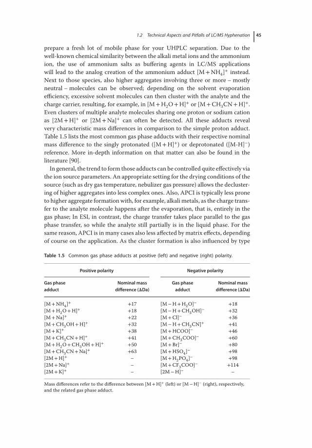
1.2 Technical Aspects and Pitfalls of LC/MS Hyphenation 45

prepare a fresh lot of mobile phase for your UHPLC separation. Due to thewell-known chemical similarity between the alkali metal ions and the ammoniumion, the use of ammonium salts as buffering agents in LC/MS applicationswill lead to the analog creation of the ammonium adduct [M+NH4]+ instead.Next to those species, also higher aggregates involving three or more – mostlyneutral – molecules can be observed; depending on the solvent evaporationefficiency, excessive solvent molecules can then cluster with the analyte and thecharge carrier, resulting, for example, in [M+H2O+H]+ or [M+CH3CN+H]+.Even clusters of multiple analyte molecules sharing one proton or sodium cationas [2M+H]+ or [2M+Na]+ can often be detected. All these adducts revealvery characteristic mass differences in comparison to the simple proton adduct.Table 1.5 lists the most common gas phase adducts with their respective nominalmass difference to the singly protonated ([M+H]+) or deprotonated ([M-H]−)reference. More in-depth information on that matter can also be found in theliterature [90].

In general, the trend to form those adducts can be controlled quite effectively viathe ion source parameters. An appropriate setting for the drying conditions of thesource (such as dry gas temperature, nebulizer gas pressure) allows the decluster-ing of higher aggregates into less complex ones. Also, APCI is typically less proneto higher aggregate formation with, for example, alkali metals, as the charge trans-fer to the analyte molecule happens after the evaporation, that is, entirely in thegas phase; In ESI, in contrast, the charge transfer takes place parallel to the gasphase transfer, so while the analyte still partially is in the liquid phase. For thesame reason, APCI is in many cases also less affected by matrix effects, dependingof course on the application. As the cluster formation is also influenced by type

Table 1.5 Common gas phase adducts at positive (left) and negative (right) polarity.

Positive polarity Negative polarity

Gas phaseadduct

Nominal massdifference (𝚫Da)

Gas phaseadduct

Nominal massdifference (𝚫Da)

[M+NH4]+ +17 [M−H+H2O]− +18[M+H2O+H]+ +18 [M−H+CH3OH]− +32[M+Na]+ +22 [M+Cl]− +36[M+CH3OH+H]+ +32 [M−H+CH3CN]+ +41[M+K]+ +38 [M+HCOO]− +46[M+CH3CN+H]+ +41 [M+CH3COO]− +60[M+H2O+CH3OH+H]+ +50 [M+Br]− +80[M+CH3CN+Na]+ +63 [M+HSO4]− +98[2M+H]+ – [M+H2PO4]− +98[2M+Na]+ – [M+CF3COO]− +114[2M+K]+ – [2M−H]− –

Mass differences refer to the difference between [M+H]+ (left) or [M−H]− (right), respectively,and the related gas phase adduct.

46 1 LC/MS Coupling

and amount of mobile phase, the signal intensity of different gas phase species canchange with the UHPLC flow rate.

In-Source Collision-Induced Dissociation Gas phase fragmentation reactions are afundamental element of mass spectrometric experiments. Imagine an analyte thatis excited to vibrations in a well-controlled manner: this molecule will then selec-tively break into pieces at the weakest bonds, thus creating a characteristic frag-ment spectrum. As long as this fragmentation reaction can be stimulated repro-ducibly, these fragmentation patterns provide you with a molecular fingerprint,which tremendously helps to identify a chemical compound. And even if you can-not afford to run your entire LC/MS experiment in full scan mode with parallelMS/MS fragmentation because you need highest sensitivity, the detection of asmany known characteristic fragments as possible in SRM mode increases the levelof confidence for your compound confirmation substantially. However, ESI andAPCI are rather mild ionization principles transferring the analyte molecules intothe gas phase as a whole, so fully intact and nonshattered – which is very differentfrom EI (also earlier known as electron impact ionization) in GC/MS. The benefitis that you will be able to determine the molecular mass of the intact molecule,but you lose the chance to learn more about the structural properties and chem-ical nature of your analyte by fragmentation patterns. Sophisticated tandem-MStechniques, however, enable you to stimulate well-controlled decomposition con-ditions in the collision cell of a tandem mass spectrometer. The user typicallyknows about the most characteristic fragments of the target analyte, so not toomany surprises are to be expected then. Many years of extensive research mean-while allowed unveiling a huge set of decomposition reactions and their follow-upsin the gas phase; a very informative and comprehensive tutorial by Holcapek et al.is a valuable starting point for your own interpretation of small molecule fragmen-tations in API mass spectrometers [90].

Next to these intended fragmentation reactions in a tandem MS, the user willalways have the chance – or the risk – to shatter the analyte in an uncontrolledway, typically stimulated by unfavorable ion source or ion transfer conditions. Aslong as the analytes have not entered the final high vacuum section of the massspectrometer, that is, while they still are in the ion source or the transfer sectionof the ion optics that come along with a staged pressure reduction, these ions willhave to remain intact in an environment where their mean free path is only in therange of a few micrometers (∼50 μm at 1 mbar of ambient pressure) and not sev-eral dozens of inches (∼20′′/500 mm for a vacuum of 10−4 mbar). A collision withexcessive ambient gas molecules is very likely there, and the higher the collisionimpulse, the more you will see an unwanted fragmentation taking place already inthe entrance area of the ion source. You can master this process to some extent bya smart selection of acceleration voltages in your ion optics. High voltages, to beapplied, for example, along the ion transfer capillary or to the skimmer electrodes,strongly accelerate the ions while traveling through the ion optics and induce moreeffective collisions with residual gas molecules, thus resulting in more fragmentsignals in the mass spectrum (also called nozzle-skimmer dissociation). In case

1.2 Technical Aspects and Pitfalls of LC/MS Hyphenation 47

of the MS method development, it is a useful approach to change the parame-ter settings for the ion source and the transfer section stepwise while monitoringthe signal change and the spectrum quality accordingly to avoid excessive ana-lyte fragmentation. However, you can also make use of this principle to artificiallystimulate ion fragmentation and to learn more about unknown compounds evenwith rather simple and cost-effective instruments such as single-quad mass spec-trometers.

A very comprehensive table on the generation of fragments out of various func-tional groups can be found in the literature [90]. We briefly discuss the behavior ofalcohols, aldehydes, and carbonic acids as representative examples for frequentlyoccurring fragmentation reactions. These compound classes have a strong het-eropolarity of the carbon–oxygen bond in common due to the high electroneg-ativity of the oxygen atom. One immediate result of this is the neutral loss ofwater; the loss of carbon oxides is another one, depending on the chemical com-position of the analyte. Once protonated in positive mode, alcohols preferablysplit off water (R-OH2

+ from R-OH), thus generating an R+ fragment (equaling[M+H−H2O]+), which is lighter than the expected ion of the intact molecularion by nominal 18 Da. Aldehydes lose carbon oxide (CO), ending up in a fragmention [M+H−CO]+. Aliphatic carbonic acids typically lose the thermodynamicallyvery stable carbon dioxide after protonation, while aromatic carbonic acids underthe same conditions preferably “only” split off water, leaving us with an acyliumcation for detection.

Contaminants Eluting from the Instrumentation Nevertheless, there will still bemany situations where a good knowledge of gas phase fragmentation reactionsand chemical expertise will not help to explain the existence of prominent masssignals in your MS spectrum: for instance, the sheer amount of mass signalsbeing so high that they cannot be deduced by fragmentation reactions, or massinterferences not only showing up as one individual signal but as a series withdistinctive patterns. The root cause here can be very trivial – contaminants areeluting from your chromatography or the mass spectrometer hardware. If yourMS was thoroughly cleaned recently, then the (U)HPLC system and any fluidicsconnected with it would be blamed for that, and the potential contaminationsources are numerous:

• Bleeding of a separation column being either old or unsuitable for MS detectionresults in an increased elution of the stationary phase bonding, which is splitoff the carrier material surface and leads to an increased noise in the LC/MSchromatogram.

• Plasticizers are ubiquitous in almost all modern plastic materials, from sam-ple vials over solvent lines, piston seals to filter frits and many other pieces.Very common plasticizers are phthalates which can rapidly be identified basedon their characteristic masses (m/z 279, 391, 413, 429, 454, and many more).Also lubricants and separating agents such as Erucamide (m/z 338, 360) canfrequently be observed.

48 1 LC/MS Coupling

• Polyethers such as polyethylene glycol (PEG) and polypropylene glycols (PPG)are another frequent contamination type, which can be identified quickly dueto their characteristic MS spectrum pattern. Also they are nearly ubiquitous inplastic materials, but they can also be introduced into the MS by working slop-pily with disposable gloves or skin care products. These compounds never showup with only one single mass signal but always come with a very characteristicpolymer distribution pattern [91]. The mass distance of the monomeric units areΔm/z= 44 for PEGs and 58 for PEGs, which immediately reveals the chemicalnature of these contaminants.

• Polysiloxanes (silicones) are core ingredients of many modern high-performance oils and vacuum grease. Oil vapor traces from the roughvacuum pump leaking into the mass spectrometer produce characteristicsignals of, for example, m/z 371, 445, or 519. In such a case, the ion optics,such as focusing multipoles or ion funnels, should be checked for cleanliness.A continuous stream of oil mist entering the MS can even lead to a razor-thinoil film coating the metal surfaces of the ion guides or, in some cases, on themass analyzer over weeks and months. This results not only in contaminantsignals in your mass spectrum but also in a measurable sensitivity loss, whichmakes a thorough and extensive cleaning mandatory in the end. But howwould it happen anyway that oil mist from the rough pump(s) could enterthe MS interior in a way that also comes along with ion generation? Well,the most obvious reason for this is a nonideal installation of the variousexhaust hoses of your MS. For convenience, the exhaust tubes of the vacuumpump(s) and of the ion source drainage are frequently tied together into thesame lab exhaust ventilation nozzle. But by doing so, you allow the vacuumpump exhaust to diffuse backward into the MS ion source and further downinto the mass spectrometer. Installing the pump exhaust and the ion sourcedraining tube into different connectors of the lab ventilation with a distanceof 1.5–3′ (0.5–1 m) in-between is a very simple and effective solution to thatissue.

• Metal ions can be a great origin for the generation of larger gas phase adductswith your target analyte molecules; alternatively, metal ions can also react withparts of your sample and thus inhibit the detection of compounds. We alreadydiscussed the formation of alkali metal adducts in section “Gas Phase Adducts”;A SST LC fluidics or massive hardware defects in a biocompatible UHPLCsystem, for example, a damaged injection valve, can result in a propagatedrelease of iron ions and thus in iron/analyte clusters in the mass spectrum;these clusters reveal themselves very quickly due to their multicharge stateand the isotope pattern of iron, which significantly deviates from those ofthe usual elements in organic matter such as carbon, hydrogen, nitrogen,and oxygen. Biochemical applications are particularly prone to issues createdby heavy metals in the mobile phase. A lot of biological compounds tend toform either precipitates or nonvolatile aggregates with iron, or alternativelyto irreversibly adsorb on iron surfaces. A frequently described phenomenonis the “vanishing,” so the nondetectability of phosphorylated peptides and

1.2 Technical Aspects and Pitfalls of LC/MS Hyphenation 49

proteins in a separation system with an SST fluidics. To avoid this, bioanalyticalapplications are preferably run on instrumentation with an iron-free fluidics,which can be made of titanium, biocompatible metal alloys like MP35N,or PEEK, with the latter being not very pressure-resistant (tubing typicallyup to 5–6000 psi/350–400 bar) and thus not being suitable for UHPLCapplications.

• Dissolved residual gases in the mobile phase, however, typically result in anunstable spray and/or interfering spikes in the LC/MS chromatogram and themass spectra rather than modifying the analyte mass signals.

The aspects discussed here can only represent a selection of some very popularphenomena, but this list is far away from being a fully comprehensive compilationof known interference signals [88]. Already some years ago, Keller et al. publishedan excellent and highly detailed, tabulated collection of all literature-known MScontaminants known at this point [92]. Most MS vendors discuss this topic veryopenly as well and compiled various collaterals on MS contamination sources [89,93], and last but not least the internet offers various public data search engineson that matter. One example to be mentioned is the MaConDa (Mass spectrome-try Contaminant Database) database maintained by the University of Birmingham[91], which allows to search for more than 300 contaminants based on accuratemass, compound class, and mass spectrometer type (operation principle and man-ufacturer), featuring also many literature references.

1.2.3.5 Instrumental Reasons for the Misinterpretation of Mass SpectraFinally, we investigate some selected instrumental reasons that can lead to themisinterpretation of mass spectra. As discussed earlier, all MS types have theirstrengths and weaknesses that affect also the quality of your analytical result. Letus discuss these in the following on three scenarios:

False Mass Assignment Depending on Ionization Principle As already discussed insection “Gas Phase Adducts”, the selected ion creation principle determineswhich m/z value is shown in your mass spectrum for an unknown analytespecies. The most frequently used ionization process by charge transfer, thatis, proton association or distraction (used in ESI and APCI), does not resultin the molecular mass of the intact molecule being measured, but in an m/zvalue differing by one proton mass (or multiple proton masses at a respectivelycorrected fraction of the intact molecule mass for multicharged molecular ions).Other processes such as APPI or EI (hardly used in LC/MS), which can createions also by transferring electrons instead of protons lead to a measured m/zvalue, which deviates from the theoretical value of the intact molecule only bythe much smaller mass amount of an electron. With ESI, APCI, and APPI, theformation of adducts with alkali metals and/or residual solvent molecules canlead to misinterpreting a numerical m/z value as representing an [M+H]+ ionspecies, which in fact would be, for instance, an [M+H2O+Na]+ ion instead.A thorough look on your mass spectrum can be very helpful here, as many

50 1 LC/MS Coupling

adduct species coexist with others, with characteristic m/z differences betweenthe various ion aggregates. So if you find a new m/z value, which you may takefor an [M+H]+ ion, just check for further signals with m/z differences to thefirst one of, say, [“M+H”+ 22]+, [“M+H”+ 38]+, or [“M+H”+ 41]+ – withthese being a sodium, potassium, and ACN/proton adduct, respectively; thisseries can additionally confirm (or disprove) your originally assumed massassignment.

False Interpretation Due to Poor Mass Resolving Power Another reason leading to amass signal misinterpretation is a poor or inappropriate mass resolution. Imag-ine two different analyte species having only very small differences in their m/zvalues and arriving in the mass analyzer simultaneously; a low-resolving massspectrometer will not be able to sufficiently discriminate the two different masses.The resulting mass spectrum will thus show only the envelope curve for the twodifferent mass patterns, and the peak maxima of this envelope function do notnecessarily have to be identical to the mass signal maxima of the mass spectrumof each individual compound. Also, low-resolution mass spectrometers will notbe able to resolve higher charge states; we know that the m/z distance betweenthe isotope pattern signals of a compound equals the 1/nth fraction of the chargestate n, which means at the same time that for analyte ions with three or morecharges the isotope pattern cannot be resolved appropriately with low-res massspecs. In summary, co-eluting contaminants or impurities could not be identi-fied as such, or mass signals are erroneously assigned to the wrong compounds.It depends – next to your budget of course – on the sample complexity and thequality of your separation how good the resolving power of your mass spectrome-ter must be at minimum. The better your chromatography, the more unambiguousthe interpretation of your mass spectrum will be in the end. As a general recom-mendation, a mass spectrometer for the determination of accurate masses shouldhave a resolving power R of 10 000–15 000 at least; the scientific literature typi-cally defines R of 10 000 as the minimum for high-resolution and R of 100 000 forultra-high-resolution mass spectrometry [75].

False Mass Determination Due to Inappropriate or Unstable Experimental ConditionsIt is an obvious fact: a mass determination is always achieved by comparing yourinstrumental MS data for the analyte with the mass signals of known calibrationstandards; thus the quality and the long-term stability of the mass calibrationare critical for a reliable mass measurement. Expired or contaminated referencestandards with partially degraded ingredients should of course not be used forcalibration anymore. An undefined number of mass signals during the masscalibration process compromises the correct mass assignment and impairsor even blocks software tools such as autotune algorithms. Once successfullycalibrated, the quality of the mass axis calibration needs to be verified regularly.As discussed earlier, TOF instruments are particularly prone to drifts in the massaxis calibration even on short-term periods of (much) less than 1 h. Hence, aninternal mass calibration by a continuous calibrant infusion is essential for a

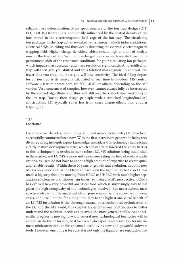
1.2 Technical Aspects and Pitfalls of LC/MS Hyphenation 51

reliable mass determination. Mass spectrometers of the ion trap design (QIT,LIT, FTICR, Orbitrap) are additionally influenced by the spatial density of theions stored in the electromagnetic field cage of the ion trap. The circulatingion packages in the trap act as so-called space charges, which induce additionalelectrical fields, shielding and thus locally distorting the external electromagnetictrapping field. Higher charge densities, which means high amount of analyteions in the trap cell and/or multiply-charged ion species, translate then into apronounced shift of the resonance conditions for your circulating ion packages,which impairs mass accuracy and mass resolution significantly. An overfilled iontrap will then give you shifted and thus falsified mass signals. In contrast, thefewer ions you trap, the more you will lose sensitivity. The ideal filling degreefor an ion trap is dynamically calculated in real time by modern MS controlsoftware – feature names here are ICC, AGC, or others, depending on the MSvendor. Very concentrated samples, however, cannot always fully be interceptedby the control algorithms and thus will still lead to a short-time overfilling ofthe ion trap. Due to their design principle with a stretched longitudinal cellconstruction, LIT typically suffer less from space charge effects than circulartraps (QIT).

1.2.4Conclusion

For almost two decades, the coupling of LC and mass spectrometry (MS) has beensuccessfully commercialized now. With the first instrument generation being truedivas requiring in-depth expert knowledge, nowadays this technology has reacheda fairly mature development state, which substantially lowered the entry barrierto this technique; this results in many robust LC/MS solutions being establishedin the market, and LC/MS is more and more penetrating the field of routine appli-cations, as users do not have to adopt a high amount of expertise to create quickand reliable results. Within these 20 years of growth and evolution, not only newMS technologies such as the Orbitrap have seen the light of day but also LC hasmade a big step ahead by moving from HPLC to UHPLC with much higher sep-aration efficiencies and shorter run times. So from a bird’s perspective, LC/MShas evolved to a very powerful analytical tool, which is surprisingly easy to usegiven the high complexity of the technologies involved. But nevertheless, massspectrometry is not the analytical all-purpose weapon as it is advertised in somecases, and it will not be for a long time. Key to the highest analytical benefit ofan LC/MS installation is the thorough mutual physicochemical optimization ofthe LC and the MS world; this chapter hopefully is one contribution to betterunderstand the technical needs and to avoid the most general pitfalls. As the sci-entific progress is moving forward, several new technological territories will beentered in the future for sure, be it for even higher speed and resolution, for instru-ment miniaturization, or for enhanced usability by new and powerful softwaretools. However, one thing is for sure: it is not only the liquid phase separation that

52 1 LC/MS Coupling

benefits from the mighty analytical information creation by mass spectrometrybut also MS technologies will massively fall short on their potential without a thor-oughly optimized chromatography upfront. For the foreseeable future, both con-cepts, chromatography and mass spectrometry, will continue to depend on eachother.

1.2.5Abbreviations

AP(C)I atmospheric pressure (chemical) ionizationCAD charged aerosol detectionCID collision-induced dissociationECD electrochemical detectionEI electron ionization (also: electron impact ionization

[obs.])EIC extracted ion chromatogramESI electrospray ionizationELSD evaporative light scattering detectorFA formic acidFIA flow injection analysisFT Fourier transformationGDV gradient delay volumeHPG high-pressure gradient pumpHR/AM high-resolution/accurate massHTS high-throughput screeningHV high voltageICR ion cyclotron resonanceI.D. inner diameterLIT linear ion trapLPG low-pressure gradient pumpMRM Multiple Reaction MonitoringMSD mass selective detectorPEEK poly(ether ether ketone)PEG poly(ethylene glycol)PPG poly(propylene glycol)QIT quadrupole ion trapSIM single-ion monitoringSRM Selected Reaction MonitoringSST stainless steelTFA trifluoroacetic acidTOF time of flight

1.3 LC Coupled to MS – A User Report 53

1.3LC Coupled to MS – A User Report

Alban Muller and Andreas Hofmann

In comparison to coupling LC to UV, coupling LC to mass spectrometry (MS)requires important adaptations. Water–methanol or water–acetonitrile gradi-ents are often applied in RP chromatography. Only volatile buffers should be usedin order to prevent contamination of the MS instrument by nonvolatile salts. Forexample, FA or acetic acid can be used for acidic conditions and ammonia can beused for alkaline conditions. If samples contain nonvolatile salts, the LC flow canbe directed to waste at the beginning of the analysis to prevent contamination ofthe MS instrument. A two-dimensional LC system with an enrichment column isanother option to analyze samples containing nonvolatile salts. Matrix effects canreduce signal-to-noise ratios of analytes in complex biological samples. Addingheavy isotope-labeled standards to samples allows to take losses during extrac-tion and matrix effects into account. 2H, 13C, and 15N are often used to isotopicallylabel standards. In contrast to 2H-labeled standards that can show small retentiontime shifts, 13C- and 15N-labeled standards elute at the same time as the analytes.

The most suitable LC system can be selected based on the required sensitivityand the desired analysis time. The MS signal intensity is proportional to theconcentration of the analyte. Nano LC systems are mainly used to achievehighest sensitivity. High sensitivity is especially critical for the analysis of lowabundant endogenous molecules, for example, in proteomics experiments.In proteomics experiments, chromatographic columns have often an innerdiameter of only 75 μm or lower. The low solvent flow rate (e.g., 250 nl/min) innano-LC/MS methods can lead to an analysis time of 1 h and more, but allowsthe most sensitive approach to detect endogenous molecules. Higher LC flowrates (400–600 μl/min) are usually applied for the detection and quantificationof analytes with higher concentrations. Chromatography columns with a 1 or2.1 mm inner diameter are often used for U(H)PLC applications that allow tocomplete an analysis in only few minutes.

The method of ionization is chosen based on analyte properties and the LCflow rate. ESI is suitable for a very broad spectrum of analytes and LC flowrates. Hydrophilic as well as hydrophobic substances can be well analyzed withESI. APCI and APPI are mainly applied for the analysis of very hydrophobicsubstances and require high LC flow rates. In general, the ion source temperatureand the gas flow rates need to be increased with increasing solvent flow rates.Recommended parameters for different LC flow rates can be found in the manualof the ion source. These recommended parameters often represent a good startingpoint for your own optimization. In addition to parameters that depend on thesolvent flow rate, analyte-dependent parameters of the ion source need to beoptimized. Analyte-dependent parameters can be optimized by direct infusionof a pure analyte solution with a syringe pump, in order to adjust all parametersfor a maximal signal-to-noise ratio. Combining the flow of the syringe pumpvia a T-piece with the LC flow allows to simulate conditions close to the final

54 1 LC/MS Coupling

analysis conditions. Relatively high concentrations of analyte have to be used fordirect infusion, which can lead to background signals of the analyte. Differentinstrument parameters can also directly be varied during the LC/MS analysis, dueto the short analysis time of U(H)PLC systems and the fast scan speed of modernMS instruments. A lower concentration of analyte can be used for the variationof parameters during the LC/MS analysis compared with direct infusion. Manysteps of the optimization can automatically be done by the instrument software orplatform-independent software. However, automatically determined parametersshould always be checked for plausibility. Orifices of MS instruments have beenenlarged over the last years in order to increase ion transmission. Not onlymore ions but also more neutral particles enter the MS instrument through theenlarged orifice; therefore, strong roughing and turbo pumps are necessary tomaintain the required vacuum. Furthermore, the geometry of the ion opticswere changed to efficiently separate ions from neutral particles, for example, byusing the StepWaveTM, iFunnel, or electrodynamic ion funnel technology. Theimproved ion transmission of modern MS instruments results in higher signal-to-noise ratios, more robust methods, and facilitated optimization of instrumentparameters.

Mass accuracy, mass resolution, scan speed, sensitivity, and many otherparameters of MS instruments can differ greatly. Some applications may onlybe feasible with one specific type of MS instrument. Basic MS instruments,such as single quadrupole, ion trap, or TOF instruments, can be used to analyzesamples with low complexity. Hybrid MS instruments, combining two massanalyzers, are often used to analyze complex biological samples. Hybrid MSinstruments with high mass accuracy and mass resolution, for example, Q-TOF,TOF-TOF, ion trap-Orbitrap, or Q-Orbitrap instruments, allow the identificationof unknown substances. Triple quadrupole MS instruments with high scanspeed and excellent sensitivity are often applied for quantitative analyses. Atriple quadrupole instrument consists of three quadrupoles arranged one afterthe other (Figure 1.12a). The first quadrupole is used as a mass filter for theionized, intact analyte. The ionized, intact analyte is also called parent ion. Theparent ion is then fragmented in the second quadrupole by collision-induceddissociation. Subsequently, the third quadrupole filters for a specific fragment ofthe parent ion, also called daughter ion. Assays on triple quadrupole instrumentsare very sensitive and selective due to the double filtering in the first and thirdquadrupole.

For example, isomers of the hydroxy-eicosatetraenoic acid are difficult to sepa-rate chromatographically (Figure 1.12b), and a simple mass analysis shows over-lapping peaks for the parent ions (Figure 1.12c). However, a triple quadrupoleinstrument enables to measure specific daughter ions of the two isomers and thedaughter ion traces show no interferences between the two isomers [94].

Ion-pairing reagents, such as TFA for acidic conditions or triethylamine foralkaline conditions, can be used for the separation of hydrophilic analytes by RPchromatography. In general, ion-pairing reagents often lead to a reduced signal-to-noise ratio and to high background signals when the polarity is switched.

1.3 LC Coupled to MS – A User Report 55

(a)

Q1 Q2 Q3

(b) (c)

OH

OH

OH

OH

O

O

m/z: 247.2

m/z: 261.2

m/z: 319.2

m/z: 319.2 → 261.2

m/z: 319.2 → 247.2

Retention time

Sig

na

l in

ten

sity

Retention time

Sig

na

l in

ten

sity

17(S)-HETE ([M−H]−= 319.2 m/z)

18(S)-HETE ([M−H]−= 319.2 m/z)

Figure 1.12 (a) Schematic representationof the quadrupoles of a triple quadrupoleinstrument. Only two quadrupole rods ofthe four quadrupole rods are shown for eachquadrupole. The first quadrupole (Q1) filtersfor the precursor ion, the precursor ion is

fragmented in Q2 by collision-induced disso-ciation and Q3 filters for a specific daughterion. (b) Isomers of hydroxy-eicosatetraenoicacid (HETE). (c) Schematic representation ofion traces by measuring just the precursorions or daughter ions of HETE isomers.

Ion chromatography (IC) is a reliable alternative to separate very hydrophilic,charged molecules, which cannot be readily analyzed by RP chromatography.Analytes are separated based on their charge and size by IC. In contrast tosilica-based RP columns, the stationary phases of IC columns are polymer-based.Therefore, IC columns are very stable under alkaline conditions. Potassiumhydroxide is often used for anion exchange chromatography, and the elutingstrength is directly proportional to the potassium hydroxide concentration.Methanesulfonic acid is often used for cation exchange chromatography.

An example of an anion exchange IC coupled to a triple quadrupole MS isdescribed in the following section. A potassium hydroxide gradient is producedby the eluent generator and analytes are separated on the IC column. There-after, potassium ions are exchanged by hydronium ions in the electrochemicalsuppressor. Usually, IC is coupled to a conductivity detector, which determinesthe conductivity of the solution. A conductivity detector is relatively insensitiveand not well suited for biological applications, for example, in the field ofmetabolomics. Furthermore, the conductivity is not selective so that analyteswith the same retention time cannot be distinguished. In contrast, a triplequadrupole instrument enables a very sensitive and selective detection of differ-ent analytes. Without electrochemical suppressor, potassium ions would lead toa strong suppression of analyte signals and contamination of the MS instrument.The electrochemical suppressor generates an aqueous solution with a low saltconcentration of a few microsiemens. The efficiency to generate negative ions

56 1 LC/MS Coupling

can be increased by adding an organic solvent, such as methanol, via a T-pieceto the aqueous solution. A Dionex ICS-3000 IC system, an ESI ion source and anAB Sciex QTrap 5500 MS instrument was used for the analysis described here.The triple quadrupole instrument allows a very sensitive and selective detectionof analytes via MS/MS experiments.

1.3.1Conditions of the Ion Chromatography

Eluent generator EGC III KOHEnrichment column Ion Pac AG20 2× 50 mmAnalytical column Ion Pac AS20 2× 250 mmColumn temperature 35 ∘CIC pump Isocratic, 250 μl/minSuppressor electric current 62 mALoop volume 2 μlMethanol flow rate 50 μl/min

1.3.2Gradient Generator

Time (min) [OH−] (mM)

0 107.5 45

17.5 4818.5 10022.5 10022.6 1025 10

1.3.3Transitions

Analyte Q1 mass (Da) Q3 mass (Da)

3-Hydroxybutanoic acid 103.1 58.9Hippuric acid 178.1 134.13-(3-Hydroxyphenyl)propanoic acid 165.0 105.9p-Cresol sulfate 186.8 106.9

1.3 LC Coupled to MS – A User Report 57

3 - Hydroxybutanoic acid

Hippuric acid

3-(3 - Hydroxyphenyl)propanoic acid

p-Cresol sulfate

58 1 LC/MS Coupling

References

1. Matuszewski, B.K., Constanzer, M.L.,and Chavez-Eng, C.M. (2003) Anal.Chem., 75, 3019–3030.

2. Annesley, T.M. (2003) Clin. Chem., 49,1041–1044.

3. McEwen, C.N., Mckay, R.G., and Larsen,B.S. (2005) Anal. Chem., 77, 7826–7831.

4. McEwen, C. and Gutteridge, S. (2007)J. Am. Soc. Mass Spectrom., 18,1274–1278.

5. Ray, A.D., Hammond, J., and Major,H. (2010) Eur. J. Mass Spectrom., 16,169–174.

6. Cody, R.B., Laramee, J.A., andDurst, H.D. (2005) Anal. Chem., 77,2297–2302.

7. Takats, Z., Wiseman, J.M., Gologan, B.,and Cooks, R.G. (2004) Science, 306,471–473.

8. Laramee, J.A. and Cody, R.B. (2007) inThe Encyclopedia of Mass Spectrome-try, Vol. 6 (eds. M.L. Gross and R.M.Caprioli), Elsevier, Amsterdam, Chapter5, 377–387.

9. Schurek, J., Vaclavik, L., Hooijerink,H., Lacina, O., Poustka, J., Sharman,M., Caldow, M., Nielen, M.W.F., andHajslova, J. (2008) Anal. Chem., 80,9567–9575.

10. Lloyd, J.A., Harron, A.F., andMcewen, C.N. (2009) Anal. Chem.,81, 9158–9162.

11. Ahmed, A., Cho, Y.J., No, M.H., Koh,J., Tomczyk, N., Giles, K., Yoo, J.S., andKim, S. (2011) Anal. Chem., 83, 77–83.

12. Pan, H.F. and Lundin, G. (2011) Eur. J.Mass Spectrom., 17, 217–225.

13. Maleknia, S.D., Vail, T.M., Cody, R.B.,Sparkman, D.O., Bell, T.L., and Adams,M.A. (2009) Rapid Commun. MassSpectrom., 23, 2241–2246.

14. Edison, S.E., Lin, L.A., Gamble, B.M.,Wong, J., and Zhang, K. (2011) RapidCommun. Mass Spectrom., 25, 127–139.

15. Krieger, S., von Trotha, A., Leung,K.S.-Y., and Schmitz, O.J. (2013) Anal.Bioanal. Chem., 405 (4), 1373–1381.

16. Cole, R.B. (ed) (1997) Electrospray Ion-ization Mass Spectrometry, John Wiley &Sons, Inc., New York.

17. Cech, N.B. and Enke, C.G. (2001) MassSpectrom. Rev., 20, 362–387.

18. Kebarle, P. (2000) J. Mass Spectrom., 35,804–817.

19. Niessen, W.M.A. (ed) (1999) LiquidChromatography – Mass Spectrometry,Marcel Dekker, Inc., New York.

20. Van Berkel, G.J., McLuckey, S.A., andGlish, G.L. (1991) Anal. Chem., 63,2064–2068.

21. Van Berkel, G.J., McLuckey, S.A., andGlish, G.L. (1992) Anal. Chem., 64,1586–1593.

22. Van Berkel, G.J. and Asano, K.G. (1994)Anal. Chem., 66, 2096–2102.

23. Van Berkel, G.J. and Zhou, F. (1995)Anal. Chem., 67, 2916–2923.

24. Van Berkel, G.J. and Zhou, F. (1995)Anal. Chem., 67, 3958–3964.

25. Van Berkel, G.J., Quirke, J.M.E., Tigani,R.A., Dilley, A.S., and Covey, T.R. (1998)Anal. Chem., 70, 1544–1554.

26. Van Berkel, G.J., Quirke, J.M.E., andAdams, C.L. (2000) Rapid Commun.Mass Spectrom., 14, 849–858.

27. Williams, D. and Young, M.K. (2000)Rapid Commun. Mass Spectrom., 14,2083–2091.

28. Quirke, J.M.E., Hsz, Y.-L., andVan Berkel, G.J. (2000) Nat. Prod.,63, 230–237.

29. Williams, D., Chen, S., and Young, M.K.(2001) Rapid Commun. Mass Spectrom.,15, 182–186.

30. Quirke, J.M.E. and Van Berkel, G.J.(2001) J. Mass Spectrom., 36, 179–187.

31. Kauppila, T.J., Kostiainen, R., and Bruins,A.P. (2004) Rapid Commun. Mass Spec-trom., 18, 808–815.

32. Rentel, C., Strohschein, S., Albert, K.,and Bayer, E. (1998) Anal. Chem., 70,4394–4400.

33. Bayer, E., Gfrörer, P., and Rentel, C.(1999) Angew. Chem. Int. Ed., 38,992–995.

34. Takino, M., Daishima, S., Yamaguchi, K.,and Nakahara, T. (2001) J. Chromatogr.A, 928, 53–61.

35. Roussis, S.G. and Proulx, R. (2002) Anal.Chem., 74, 1408–1414.

36. Marwah, A., Marwah, P., and Lardy, H.(2002) J. Chromatogr. A, 964, 137–151.

References 59

37. Singh, G., Gutierrez, A., Xu, K., andBlair, I.A. (2000) Anal. Chem., 72,3007–3013.

38. Higashi, T., Takido, N., Yamauchi, A.,and Shimada, K. (2002) Anal. Sci., 18,1301–1307.

39. Higashi, T., Takido, N., and Shimada, K.(2003) Analyst, 128, 130–133.

40. Hayen, H., Jachmann, N., Vogel, M.,and Karst, U. (2002) Analyst, 127,1027–1030.

41. Zwiener, C. and Frimmel, F.H. (2004)Anal. Bioanal. Chem., 378, 851–861.

42. Syage, J.A. and Evans, M.D. (2001) Spec-troscopy, 16, 15–21.

43. Syage, J.A., Hanold, K.A., Evans, M.D.,and Liu, Y. (2001) Atmospheric pressurephotoionizer for mass spectrometry.Patent no. WO0197252.

44. Robb, D.B., Covey, T.R., and Bruins, A.P.(2000) Anal. Chem., 72, 3653–3659.

45. Robb, D.B. and Bruins, A.P. (2001).Atmospheric pressure photoioniza-tion (APPI): A new ionization methodfor liquid chromatography – massspectrometry. Patent No. WO0133605.

46. Baim, M.A., Eartherton, R.I., andHill, H.H. Jr., (1983) Anal. Chem., 55,1761–1766.

47. Leasure, C.S., Fleischer, M.E., Anderson,G.K., and Eiceman, G.A. (1986) Anal.Chem., 58, 2142–2147.

48. Spangler, G.E., Roehl, J.E., Patel,G.B., and Dorman, A. (1994). U.S.Patent no. 5,338,931.

49. Kauppila, T.J., Kuuranne, T., Meurer,E.C., Eberlin, M.N., Kotiaho, T., andKostiainen, R. (2002) Anal. Chem., 74,5470–5479.

50. Discroll, J.N. (1976) Am. Lab., 8, 71–75.51. Discroll, J.N. (1977) J. Chromatogr., 134,

49–55.52. Locke, D.C., Dhingra, B.S., and Baker,

A.D. (1982) Anal. Chem., 54, 447–450.53. Zeleny, J. (1917) Phys. Rev., 10, 1–6.54. Wilson, C.T.R. and Taylor, G. (1925)

Proc. Cambridge Philos. Soc., 22,728–730.

55. Taylor, G. (1964) Proc. R. Soc. LondonSer. A, 280, 383–397.

56. Dole, M., Mack, L.L., Hines, R.L.,Mobley, R.C., Ferguson, L.D., andAlice, M.B. (1968) J. Chem. Phys., 49,2240–2249.

57. Yamashita, M. and Fenn, J.B. (1984) J.Phys. Chem., 88, 4451–4459.

58. Cole, R.B. (2000) J. Mass Spectrom., 35,763–772.

59. Kebarle, P. and Peschke, M. (1994) Anal.Chem., 66, 712–718.

60. Thomson, B.A. and Iribarne, J.V. (1979)J. Chem. Phys., 71, 4451–4463.

61. Molin, L. and Traldi, P. (2007) in: A.Cappiello (ed), Advances in LC–MSInstrumentation, Basic aspects of elec-trospray ionization, J. Chromatogr. Libr.,Elsevier, Amsterdam, 72 Kapitel 1,S1–S9.

62. Carrol, D.I., Dzidic, I., Stillwell, R.N.,Horning, M.G., and Horning, E.C. (1974)Anal. Chem., 46, 706–710.

63. Moini, M. in: Gross, M. L. and Caprioli,R. M. (eds) (2007) The Encyclopedia ofMass Spectrometry, Atmospheric Pres-sure Chemical Ionization: Principles,Instrumentation, and Applications,Vol. 6, Chapter 5, Elsevier, Amsterdam,pp. S344–S354.

64. Lias, S.G. (2003) Ionization energy eval-uation, in NIST Chemistry WebBook,NIST Standard Reference DatabaseNumber 69 (eds P.J. Linstrom and W.G.Mallard), March 2003, National Instituteof Standards and Technology, Gaithers-burg, MD, 20899 (http://webbook.nist.gov).

65. Raffaelli, A. and Saba, A. (2003) MassSpectrom. Rev., 22, 318–331.

66. Klee, S., Albrecht, S., Derpmann, V.,Kersten, H., and Benter, T. (2013) Anal.Bioanal. Chem., 405, 6933–6951.

67. Kauppila, T.J., Kotiaho, T., Kostiainen,R., and Bruins, A.P. (2004) J. Am. Soc.Mass Spectrom., 15, 203–211.

68. Constapel, M., Schellenträger, M.,Schmitz, O.J., Gäb, S., Brockmann,K.-J., Giese, R., and Benter, T. (2005)Rapid Commun. Mass Spectrom., 19,326–336.

69. Tian, N., Thiessen, A., Schiewek, R.,Schmitz, O.J., Hertel, D., Meerholz, K.,and Holder, E. (2009) J. Org. Chem., 74,2718–2725.

70. Schiewek, R., Mönnikes, R., Wulf, V.,Gäb, S., Brockmann, K.J., Benter, Th.,and Schmitz, O.J. (2008). Angew. Chem.Int. Ed. 47, 9989–9992 and (2008)Angewandte Chemie 120, 10138–10142.

60 1 LC/MS Coupling

71. Schiewek, R., Schellenträger, M.,Mönnikes, R., Lorenz, M., Giese, R.,Brockmann, K.-J., Gäb, S., Benter, T.,and Schmitz, O.J. (2007) Anal. Chem.,79, 4135–4140.

72. Schiewek, R., Lorenz, M., Brockmann,K.J., Benter, T., Gäb, S., and Schmitz,O.J. (2008) Anal. Bioanal. Chem., 392,87–96.

73. Makarov, A. (2000) Anal. Chem., 72,1156–1162.

74. Perry, R.H., Cooks, R.G., and Noll,R.J. (2008) Mass Spectrom. Rev., 27,661–699.

75. Holcapek, M., Jirasko, R., and Lisa, M.(2012) J. Chromatogr. A, 1259, 3–15.

76. de Hoffmann, V. and Stroobant, V.(2009) Mass Spectrometry – Principlesand Applications, 3rd edn, John Wiley &Sons Ltd, Chichester, West Sussex.

77. Rogatsky, E., Zheng, Z., andStein, D. (2010) J. Sep. Sci., 33,1513–1517.

78. Thermo Fisher Scientific (2016)ViperTM Fingertight Fitting, [Online],http://www.thermoscientific.de/products/fingertight-zero-dead-volume-fittings.html (accessed onJanuary 30, 2016).

79. Agilent Technologies (2015) A-Line Fit-tings, [Online], http://www.agilent.com/en-us/products/liquid-chromatography/lc-supplies/capillaries-fittings/a-line-fittings (accessed on January 30, 2016).

80. MicroSolv Technology Corporation(2015) Sure-Fit Connectors, [Online],https://www.idex-hs.com/column-hardware/connectors/sure-fittm-connectors.html (accessed on January30, 2016); IDEX Health & Science (2016)MarvelX, [Online], https://www.idex-hs.com/marvelx (accessed on January 30,2016).

81. Rodriguez-Aller, M., Gurny, R.,Veuthey, J.-L., and Guillarme, D.(2013). J. Chromatogr. A 1292, 2–18,10.1016/j.chroma.2012.09.061 (accessedon December 11, 2015).

82. Schappler, J., Nicoli, R., Nguyen, D.,Rudaz, S., Veuthey, J.-L., and Guillarme,D. (2009) Talanta, 78, 377–387.

83. Hopfgartner, G., Bean, K., and Henion, J.(1993) J. Chromatogr., 647, 51–61.

84. Asperger, A., Efer, J., Koal, T., andEngewald, W. (2001) J. Chromatogr. A,937, 65–72.

85. Dams, R., Benijts, T., Günther, W.,Lambert, W., and De Leenheer, A.(2002) Rapid Commun. Mass Spectrom.,16, 1072–1077.

86. Hoffmann, T. and Martin, M.M. (2010)Electrophoresis, 31 (7), 1248–1255.

87. Gosetti, F., Mazzucco, E., Zampieri, D.,and Gennaro, M.C. (2010) J. Chromatogr.A, 1217, 3929–3937.

88. Guo, X.H., Bruins, A.P., and Covey, T.R.(2006) Rapid Commun. Mass Spectrom.,20 (20), 3145–3150.

89. Agilent Technologies (2015) WhatAre the Common Contaminants inMy GCMS. [Online] Link: http://www.agilent.com/cs/library/Support/Documents/FAQ232%20F05001.pdf(accessed on January 30, 2016).

90. Holcapek, M., Jirasko, R., and Lisa,M. (2010) J. Chromatogr. A, 1217,3908–3921.

91. MaConDa Mass Spectrometry Contam-inant Database [Online] Link: http://www.maconda.bham.ac.uk/search.php(accessed on January 30, 2016).

92. Keller, B.O., Suj, J., Young, A.B., andWhittal, R.M. (2008) Anal. Chim. Acta,627 (1), 71–81.

93. Waters Corporation (2015) ESI+ Com-mon Background Ions. [Online] Link:http://www.waters.com/webassets/cms/support/docs/bkgrnd_ion_mstr_list.pdf(accessed on January 30, 2016).

94. Dumlao, D.S., Buczynski, M.W., Norris,P.C., Harkewicz, R., and Dennis, E.A.(2011) High-throughput lipidomic anal-ysis of fatty acid derived eicosanoidsand N-acylethanolamines. Biochim. Bio-phys. Acta, 1811 (11), 724–736. doi:10.1016/j.bbalip.2011.06.005

61

2Optimization Strategies in RP-HPLCFrank Steiner, Stefan Lamotte, and Stavros Kromidas

2.1Introduction

Optimization of devices and processes is very common in today’s efficiency-oriented world with everyone striving to do things faster but with no loss ofquality. It is, therefore, important to define the best approach in which optimiza-tion can be achieved and how the related quality can also be measured. There arenumerous parameters in a technique such as HPLC of either independent of eachother or that have a related nature to other parameters. Optimization goals canvary and mostly depend on specific needs of analytical laboratories. The mostimportant optimization criteria in HPLC will be elucidated and discussed in thisintroductory section.

It is important to note that the majority of rules in this chapter on optimizationare valid beyond reversed phase (RP) separation mechanisms, though most of thegiven examples are based on RP-HPLC and the same applies for the concepts onselectivity optimization. In spite of a rapid development of mixed-mode phase-based and HILIC separations, RP continues to be the most widespread separationmode in modern HPLC and UHPLC.

2.1.1Speed of Analysis

Speed is the most common HPLC optimization criterion. A method is consideredoptimized if it allows the separation of all relevant components with sufficient res-olution in the shortest time possible. Such speed increase only translates into aneconomical benefit for the laboratory if it actually enables productivity increase ofthe respective lab. Labs with particularly high sample load are typical beneficiariesof this, but so are all labs that directly profit from knowing analytical results withinhours or even minutes after receiving the samples in order to react on it. Produc-tivity increase often requires optimization of the entire lab workflow which willinclude more than the analytical separation process. It is rather common that sam-ples do not arrive in a ready to inject format and thus require sample preparation

The HPLC Expert: Possibilities and Limitations of Modern High Performance Liquid Chromatography,First Edition. Edited by Stavros Kromidas.© 2016 Wiley-VCH Verlag GmbH & Co. KGaA. Published 2016 by Wiley-VCH Verlag GmbH & Co. KGaA.

62 2 Optimization Strategies in RP-HPLC

steps. If the time to perform these steps cannot be optimized to a similar extent,they will become the bottleneck in the workflow. Consequently, faster separationsmay only be of very limited benefit for the overall productivity.

In-process analysis depends very often on fast analysis, no matter on where thisoccurs – either research or production processes, continuous or batch processes.A reduction in the analysis time always results in a higher information density,which normally translates into an economical benefit downstream. It is an inter-esting notion the speed potential of modern UHPLC finally enabled the use ofliquid chromatography for current in-process analysis, but is yet very rarely foundthere.

2.1.2Peak Resolution

The resolution between neighboring peaks is another common optimization goal.There are two approaches to influence resolution in chromatography:

• increasing column efficiency• improving the selectivity, by changing the relative retention times of the respec-

tive components.

Optimizing the resolution enhances the accuracy and precision of quantitativeanalysis and can also improve method robustness. It can even reduce the amountof sample preparation provided that the optimized method can handle a directinjection of samples with more complex matrices. Improved separation efficiencyalso translates into a higher number of components that the method is able toseparate, the so-called theoretical peak capacity. Economical benefit may resultfrom simplified workflows with less sample preparation and improved data qualityto account for more accurate analyses.

2.1.3Limit of Detection and Limit of Quantification

The limit of detection (LOD) is the smallest amount of a specific analyte thatis visible with given significance. It is an important parameter for trace analy-sis. A distinction between the lowest concentration of the analyte in the sample(relative value) and the smallest absolute amount that can be detected with therespective method is important. This also has to take the type of detector intoaccount that can either be concentration dependent or amount/mass dependentin its signal generation. The latter type of detectors is in general destructive inthat it is not possible to recover the sample. With concentration-dependent detec-tors, such as the common UV absorbance detector, the concentration detectionlimit can only be improved on the detector itself, while the absolute detectionlimit depends both on the detector and on the column dimension and separa-tion efficiency. For truly mass proportional detectors, the column dimension does

2.1 Introduction 63

not matter as long as the flow rate does not affect the sensitivity of the detec-tor. Zone-sharpening effects in gradient elution help to improve both limits on alltypes of detectors. It can be concluded from these considerations that limits ofdetection are in no way a simple matter in liquid chromatography. The smallestconcentration or mass of analyte that can be quantified with a given accuracy isthe limit of quantification (LOQ). All considerations for the LOD apply, respec-tively. Optimization of these parameters can also save sample preparation steps(such as preconcentration) and improve quality of trace analysis results. Reducingsample preparation will speed up the total analysis workflow and can also elimi-nate sources of error, in particular if these steps were manually done in the originalmethod.

2.1.4Costs of Analysis

In terms of direct costs, these are primarily defined by the required consumables,for example, columns, solvents, chemicals, disposable filters, and cartridges, butalso include the often significant costs for their disposal. Other cost types aremaintenance and service, instrument amortization (or leasing) costs, and lastbut not least labor costs. For a fair comparison, the total costs per successfullyanalyzed sample must be calculated. This is achieved by dividing the sum of theabove-mentioned cost types per period (e.g., month or quarter) by the numberof analyzed samples in that period. If an instrument is used for more than onemethod, however, it is obviously more difficult to determine the cost of analysisfor one specific method. Cost reduction by solvent savings is a very effectiveway and also reduces the environmental footprint. It can be achieved throughreduction of the column diameter and also through shortening of column lengthcombined with increasing stationary phase efficiency. The related savings can becounteracted by the cost of columns. Modern volume-minimized and efficiency-optimized UHPLC columns are mostly more expensive than conventional LCcolumns, but do not necessarily allow more analyses over a column lifetime. Evenif the column cost per injection increases, this must be considered against theextra savings associated with faster analysis and higher productivity.

It should not be overlooked that highly optimized UHPLC separation meth-ods may require more thorough sample preparation than a method with a moreforgiving classical column. The extra sample preparation can result in a solventmismatch effect if the analyte gets dissolved in a very strong solvent (e.g., DMSOin RP-HPLC), which has to be corrected by solvent removal and reconstitutionof the sample. It is also possible that additional filtration or dilution steps areneeded with UHPLC. In some cases, and depending on how this dilution andsolvent transfer is executed, this will result in additional solvent consumptionand increased environmental footprint. If consumable and disposal costs in totalare higher after such an optimization from conventional LC to UHPLC, the pro-ductivity increase and data quality improvement should still clearly justify thechange.

64 2 Optimization Strategies in RP-HPLC

2.2LC Fundamentals

This section describes the fundamental relationships that are required to under-stand the rationale behind optimization of LC separations and to make predictionsbased on a theoretical understanding. For experienced users, it is an opportunityto add to their knowledge, as well as being a timely revision lesson on some of themore fundamental aspects. Beginners should refer to a text book that addressesHPLC knowledge from the scratch [1], since the understanding of the chromato-graphic process and the functional parts of the HPLC instrument is a premise.

Readers that tend to shy away from mathematics will possibly not initially enjoythis chapter, however and with time they will certainly recognize how formula andparticularly rules of thumb derived thereof can be very beneficial for a systematicapproach to optimization as opposed to trial-and-error experiments.

2.2.1Peak Resolution

The resolution RS of two substance zones recorded as a chromatogram is definedby the quotient of the peak apex distance (expressed by the difference in retentiontimes) and the average width at the peak base wb. It is calculated by 2.1 as follows:

RS =tR2 − tR1

(w1 + w2)∕2(2.1)

Resolution optimization is not equivalent to maximizing resolution, but is aboutfinding the most appropriate resolution that is just sufficient for an error-free androbust peak integration to account for accurate quantitative results. The sketchof asymmetrical peak shapes shown in Figure 2.1b is more representative for areal-world chromatogram than peaks that follow a Gaussian distribution. Nev-ertheless, the Gaussian peak shape is the foundation for the calculation of platenumbers and plate height equivalents in chromatography. If two peaks exhibitideal Gaussian shape and are of similar height, a resolution of RS = 1.5, equivalentto a 6𝜎 distance of the peaks (six times the standard deviation of the concentrationdistribution in each zone) is considered sufficient for quantitative analysis. Underthese conditions, only 2% of the peak area overlaps with the respective adjacentpeak. As real world chromatograms mostly exhibit less symmetrical peaks thatcan be of significantly different height, a minimum resolution of 1.8 is recom-mended for a robust method, and some work instructions even define an RS = 2.0requirement. It should also be noted that most USP methods suggest RS = 2.0 asthe minimum resolution. Statistics can prove though that any resolution increasebeyond RS = 2.0 will not further improve the accuracy of peak integration, but maynegatively affect analysis times.

It is very helpful for any effective separation optimization in chromatographyto know how the resolution RS of two neighboring peaks depends on the threefundamental parameters. These are the plate number N , the retention factor k, andthe separation factor 𝛼. Let us make sure we understand these parameters well.

2.2 LC Fundamentals 65

tR2

tR2

tR1

tR1W1 W2

Peak 1

Time Time

Peak 2

Sig

na

l

Sig

na

lW1

Δt

W2(a) (b)

Figure 2.1 Schematic representation of ideally symmetrical (a) and real world asymmetrical(b) peak pairs and how the resolution is calculated.

The plate number N is a compound-specific measure (it, therefore, appliesto each individual peak) for the separation efficiency of a column under clearlydefined mobile phase and temperature conditions. It will change over the columnlifetime and can also be influenced by the HPLC instrument. The plate numberincreases proportional to the column length L, provided all other conditionsremain constant (except for the column pressure). It also increases at constantcolumn length when the stationary phase particle size, particle architecture, orbonding chemistry is optimized in way that accounts for less band dispersion.The respective columns exhibit increased separation efficiency per unit columnlength. Once the plate number of a column or method is increased, one can sep-arate more analytes or separate analytes with better resolution under otherwiseconstant conditions. The formula to calculate the plate number from the peakparameters retention time tR and peak width at base wb or peak width at halfheight wh is as follows:

N = 16•

( tRwb

)2

= 5.54•

( tRwh

)2

(2.2)

The retention factor k was defined as a retention parameter that is in contrastto the retention time tR independent of column dimensions and the mobile phaseflow rate F . It is characteristic for the given analyte under given stationary andmobile phase conditions as well as temperature. The retention factor can bederived from the peak retention time tR and the column hold-up time tM (elutiontime of a nonretained compound, the so-called inert marker) and equals the ratioof the so-called net retention time tR

′ (difference of retention time and hold-uptime) and the hold-up time:

66 2 Optimization Strategies in RP-HPLC

k =tR − tM

tM=

t′RtM

(2.3)

Of highest importance for the separation of two compounds is their relativeretention. This is commonly calculated for two neighboring peaks and is definedas the separation factor 𝛼, often referred to as selectivity 𝛼. The separation factorby definition is never negative, so the two considered peaks have to be assignedaccordingly. The higher the separation factor 𝛼, the easier two compounds can beseparated under otherwise constant conditions. If the goal is to characterize themethod considering the relative retention of a compound pair, the parameter 𝛼 isnamed the selectivity of the method for the respective substances. The selectivityof LC methods is the most important parameter when it comes to peak resolutionoptimization. It equals the ratio of the retention factors (or net retention times) ofthe two peaks and can thus be easily calculated as follows:

𝛼 =t′R2

t′R1=

k2k1

(2.4)

Equation 2.5 shows how the peak resolution depends on these three parametersand can be viewed as the most important equation in chromatography. It considersthe combination of the factors that drive the separation (retention and selectivity)and the counter-productive but inevitable band dispersion. The band dispersionin relation to the path length of the separation column is expressed as the columnplate number N , where a high plate number accounts for low dispersion on a givencolumn length.

RS = 14

•√

N2•k2

1 + k2•𝛼 − 1𝛼

(2.5)

The next section discusses how the variation of the three parameters affectsthe resulting resolution of adjacent peaks. This is expressed in the three overlaidcurves in Figure 2.2. The respective ranges of the parameters (x-axis) as well as theconstant value of the respective remaining two parameters is deliberately chosento highlight the importance of each parameter appropriately and to reflect typicaland realistic values of 𝛼, k, and N .

Thus, the constant values for each parameter are as follows:

• Separation factor= 1.05• Retention factor= 5• Efficiency= 5000.

The intersection of the three curves allows the constant values of all the param-eters to be deduced.

The scale of the individual axes is chosen to accommodate the fullest range thatcould be anticipated for each of these parameters. It should be mentioned thoughthat gradient elution is much more recommendable to separate complex mixturesrather than distributing them up to a retention factor of 25 in an isocratic run.Plate numbers up to 25 000 per column are demanding to achieve in conventionalLC but readily available in modern UHPLC. The continuously strong slope of the

2.2 LC Fundamentals 67

0.0

0.5

1.0

1.5

2.0

2.5

3.0

N

kRe

so

lutio

n

RS

1.00 1.05 1.10 1.15 1.20 1.25

0 5000 10000 15000 20000 25000

0 5 10 15 20 25

N

k

α

α

Figure 2.2 Curves to demonstrate the individual influence of the three parameters selectiv-ity 𝛼, plate number N, and retention factor k on peak resolution. The constant value of therespective two remaining parameters can be read from the intersection point.

curve for the selectivity 𝛼 over the relevant range up to 1.25 shows the impor-tance and dynamics of this parameter. It should be mentioned that the selectivitycurves also saturates above values of 4, but such high separation factors betweentwo adjacent peaks are rare in practice and completely useless for productive chro-matographic separations.

The retention factor can be well controlled in liquid chromatography. Beyondthe stationary phase, it strongly depends on the composition of the mobile phaseand the temperature. As a general rule, it should never be smaller unity (k = 1),as the range from 0 to 1 in real samples is often affected by matrix components.Moreover, the resulting resolution drops markedly below k = 1, and as can be seenin Figure 2.2 it already reaches 50% of its maximal contribution at this level. Atk = 2, it rises to 67% and above k = 5 the increases of resolution is only marginaland can no longer justify the longer analysis time that comes with it.

The contribution of the plate number, N , on RS is a square root function, result-ing in continuously decreasing slope without saturation. Doubling the plate num-ber always increases the resolution by factor 1.4.

An important fact becomes very obvious from Figure 2.2: The most effectiveparameter for resolution optimization in LC is selectivity. This considerationbecomes even more important in relation to gas chromatography (GC). Basedon the much stronger intermolecular forces in liquid phases, it is easier togenerate differences in retention and a multitude of parameters based on mobilephase composition enable control this. In GC, there is a completely differentsituation as temperature is the only parameter to influence retention once thestationary phase is defined. To compensate for smaller selectivities GC column

68 2 Optimization Strategies in RP-HPLC

Increase of k

Increase of N

Increase of α

Orignal chromatogram

Figure 2.3 Influence of a change in k, N, and 𝛼 on the chromatogram for a critical peakpair.

can achieve impressive plate numbers. Even in conventional capillary GC with250 μm diameter columns, plate numbers of 200 000 are readily accessible, thanksto column lengths of up to 100 m. This is different in conventional HPLC where itis even challenging to exceed plate numbers of 10 000 in methods with equivalentanalysis times. Modern UHPLC with coupled column chains can do this up toplate numbers of 100 000. This is once again easily outperformed by modernGC with 100 μm diameter thin-layer columns run at temperatures above 300 ∘C.Those can easily generate 1 000 000 theoretical plates.

The conclusion is straightforward, but of paramount importance: GC separatesprimarily through plates, LC primarily through selectivity. This finding points tothe importance of understanding the basics of selectivity optimization very well. Itimplies both an excellent knowledge of the multitude of stationary phases as wellas the influences of mobile phase composition.

The influence of the three variables k, N , and 𝛼 on the look of a critical peak pairin a chromatogram is illustrated in Figure 2.3. To close this section, we summarizethe importance of these parameters, weigh them against each other, and discusswhat to do when.

1) The selectivity 𝛼 is the most important parameter of the three and shouldalways be addressed first to optimize resolution. It describes the differencein interaction of two analytes with a stationary phase under given elutingconditions (mobile phase and temperature). A certain difference in the inter-action is a fundamental prerequisite for a chromatographic separation. It can

2.2 LC Fundamentals 69

be influenced by many parameters, but there are hardly any rules for a system-atic optimization with guaranteed success. Users mostly optimize selectivitybased on experience gained through previous trial and error approaches; how-ever, software-assisted optimization workflows for this purpose are increasingin popularity. The latter are sometimes applied in a systematic design of exper-iment (DoE) approach to account for quality by design (QbD).

2) If the user fails to find conditions to improve selectivity for critical pairs, theincrease of plate number N provides the best alternative strategy for opti-mizing resolution. The advantage of this approach is a clear prediction of therequired boost in N to achieve a given resolution under constant selectiv-ity, so the optimization can be made very systematically. The prerequisite is,however, the availability of a column with better efficiency (normally througha smaller particle size) but equivalent selectivity. The most straightforwardway would be to increase the column length, but this also increases analysistime. In any case, will the optimization of N imply the investment for anothercolumn?

3) The last choice to optimize RS is the (nonselective) increase of interaction ofboth analytes. This is mostly the application of a mobile phase with weakerelution strength that directly leads to increase of the retention factors k1 andk2. This ranking is based on the assumption that the retention factor for thefirst eluting peak is larger than 1 in the original method with insufficientresolution. The increase in retention is always accompanied by an increase inanalysis time and above k = 3 it is only of marginal impact on resolution.

It is important to note that all the above-mentioned rules and calculations arestrictly limited to isocratic methods. In gradient elution, the parameters k, 𝛼, andN do not follow the given definitions, and the slope and shape of the gradient isof critical importance for peak shape and resolution. The fundamental consider-ations still apply, but modified parameters need to be taken into account for themathematical description (also see Chapter 3 on gradient elution).

2.2.2Optimization of Efficiency (The Kinetic Approach)

This section teaches us that the so-called kinetic optimization is the key strategyto achieve a given resolution in a shorter time. It can be expressed in a quanti-tative way as the ratio of theoretical plates per unit time. It is, therefore, crucialto understand on the variables that affect the plate number, N . We first definethe height equivalent to one theoretical plate (also called plate height), H , whichis characteristic for a stationary phase, eluting condition, and analyte combina-tion, but independent of the column length L. The plate height, H , can not onlybe easily calculated from plate number, N , and column length, L, but can also bedetermined directly from peak width and retention time:

H = LN

= L16

•

(wbtR

)2

= L5.54

(whtR

)(2.6)

70 2 Optimization Strategies in RP-HPLC

The plate height observed in modern UHPLC is in the single-digit microme-ter range, and it corresponds to the length increment of one theoretical plate onthe column in the direction of the mobile phase flow. The plate height is a goodmeasure for band dispersion. Kinetic optimization is thus related to minimizingplate heights. The flow rate, F , is an important parameter in this optimization. Inthe early days of HPLC, this was mostly neglected, but the advent of UHPLC hasemphasized its importance over the last decade. Increasing F directly increases thespeed of analysis. If it was only about increasing F deliberately to make separationsfaster, things would be easy; however, this is not the case in reality. To understandthe related implications, we will not consider the flow rate, but rather the linearvelocity, u. This parameter is not so common for users, mainly because it cannotbe set directly at the instrument. As it is independent of the column diameter andstationary phase properties, it is the more suitable measure for a straightforwarddiscussion of kinetic optimization. The linear velocity, u, is the speed at which theliquid mobile phase travels along the column and is mostly given in millimeterper second. To calculate u from the set flow rate given in milliliter per minute, thefollowing equation applies:

u = 66.67•Fd2

C•𝜋•𝜀T

(2.7)

The internal diameter dC is inserted in millimeter, and 𝜀T is the total poros-ity of the interior of the separation column. It is a dimensionless ratio betweenthe volumes occupied by the mobile and stationary phase inside the column andfor modern columns packed with spherical, porous stationary phases has a valuearound 0.7. Another way to calculate u is based on the hold-up time simply by thequotient L/tM. This is intuitive as tM is the time that the nonretained analyte needsto travel the length L of the column.

The important relationship between the band dispersion (expressed as plateheight H) and the linear velocity u is shown in Figure 2.4. It can be described byan equation that is mostly referred to as the van Deemter equation. The originalvan Deemter equation [2] was developed for GC with packed columns, but in thisvery general form it is valid for LC and GC to calculate H/u curves:

H = A + Bu+ C•u = 2𝜆dp +

2𝛾Dmu

+𝜔dp2

Dm•u (2.8)

We will not need to discuss the factors 𝜆, 𝛾 , and 𝜔 to a greater extent as they donot vary significantly, cannot be influenced by the user, and are not necessary forunderstanding the fundamental relationships. It is important to understand themeaning of the diffusion coefficient (or diffusivity) Dm and the stationary phaseparticle diameter dp. The diffusion coefficient describes the speed of diffusion ofthe analyte in the mobile phase (in this simplified approach both inside and out-side the stationary phase pores). It depends on the molecular properties of theanalyte, as well as on the temperature-dependent viscosity of the mobile phase.While the particle diameter is fixed with a given column, the diffusion coefficientcan be altered without the need to change the column. It can change with the

2.2 LC Fundamentals 71

Linear velocity u

Longitudinal diffusion B/u

Solute movement

Mass

transfe

r resis

tance

C· u

Eddy dispersion A

Pla

te h

eig

ht H

A

B

C

u

u

u

Figure 2.4 The three terms of the van Deemter equation expressed in individual curves andthe fluidic explanation in related sketches.

mobile phase composition and the column temperature, because both parame-ters influence the mobile phase viscosity. There are more advanced versions of thevan Deemter equation that distinguish between the diffusion inside and outsidethe stationary phase, but for the considerations made in this chapter, the simplifiedversion as shown in 2.8 is sufficient.

The equation shows that the first term, A, is independent of the linear velocityu and grows proportional to the particle diameter dp. The term C grows pro-portional to the linear velocity u and even grows with the square of the particlediameter dp. The remaining term B is also independent of the particle diameterbut is inversely proportional to the linear velocity; hence it decreases with increas-ing speed of the separation. The physicochemical background of the three termsof the equation is elucidated in Figure 2.4 through the sketches next to the threeindividual curves of the terms A, B, and C.

2.2.2.1 The Term Describing the Eddy Dispersion (A-Term)

The eddy dispersion term relates to the band broadening not only based on thedifferent distances that analytes have to migrate around the particles, but also dueto following a countercurrent movement in the eddy streams between the parti-cles. It is often considered independent of the linear velocity and we also treat itlike this, though there are other equations that consider a dependence on u with apower smaller than unity. The A-term grows with increasing particle diameter asthe amount of length differences grow with that. It also depends on the packingtechnique and surface properties and is small when the particle size distributionis very narrow. All these effects are represented in the factor 𝜆 that is neverthelessclose to unity.

In a nutshell: The A-term is small (good for small band dispersion) if the particlesize is small, the particle size distribution is narrow and the packing structure is

72 2 Optimization Strategies in RP-HPLC

homogeneous. All these conditions can only be controlled by the column manufac-turer.2.2.2.2 The Term Describing the Longitudinal Diffusion of Analyte Molecules (B-Term)The B-term represents the band broadening due to the diffusion of the moleculesin and against the direction of the mobile phase flow. This can be imaginedquite easily as the broadening of a zone in the column after stopping the flow.In this scenario, the band would spread over time as the concentration of theanalyte gradually equilibrates throughout the column. It is obviously a function ofthe time the analyte spends in the column; however, this is dominated by thetime the analyte spends in the mobile phase as there is a much slower diffusionin the immobilized state on the surface of the stationary phase. The longitudinaldiffusion is, therefore, inversely proportional to the linear velocity and thusdisappears with very fast separations that do not leave the analyte sufficient timefor this (diffusion in liquid phases is generally rather slow).

2.2.2.3 The Term Describing the Hindrance of Analyte Mass Transfer (C-Term)To understand the hindrance of the transfer of analytes between the mobile phaseand especially the porous stationary phase, it is important to note that there ispractically no flow of the mobile phase through the pores of the packing mate-rial. This is because of the far higher viscous friction in the much smaller channelsthat exist in the pores compared with the channels between particles. In general,the difference in size is about 1000. The mobile phase in the pores is consideredstagnant and not actively moving. This implies that the analyte molecule cannotbe actively transferred into the pores by the pressure-driven flow of the mobilephase. At the same time, the stationary phase inside the pores is of paramountimportance for the chromatographic retention, as by far the majority of station-ary phase is situated there, and only a negligible portion is outside the pores atthe outer particle surface. The pores are filled with mobile phase and there is con-tinuous exchange of this liquid, but not by a mechanical-driven transport fromthe pressure gradient. The driving force for the exchange is diffusion, which isvery dependent on the concentration gradient between the channel and the pore.This diffusion transfers the analyte molecules into the pores and hence onto thestationary phase. The diffusion is, of course, bi-directional. It first occurs towardthe stationary phase at a distinct position in column where the moving analytezone arrives, and as soon as the zone is moving further ahead, the concentrationgradient is inverted and the direction of diffusion is oriented away from the sta-tionary phase and out of the pores. This diffusion can be considered approximatelyradial in the column, hence orthogonal to the mobile phase movement and it iscrucial that this mass transfer can keep pace with the speed of the mobile phasepassing through the column. The more this diffusion lags behind the mobile phaseflow, the further the analyte zone in the mobile phase will move ahead of therespective zone in the stationary phase and the more the overall zone is broadened.This is a very important effect in chromatography and is the reason for increasedband dispersion (increase of plate height, H) when speeding up chromatographicseparations by increasing the flow rate, F.

2.2 LC Fundamentals 73

At this point, the stationary phase particle diameter is extremely important forthe kinetic optimization of separations. A smaller particle diameter reduces thedistance for the necessary radial diffusion of analyte molecules on the one hand,but increases the geometrical radial concentration gradient that drives the diffu-sion. Both effects are synergistic for an efficient analyte transport and this is thephysicochemical foundation for the decrease of the C-term with the squared parti-cle diameter (dp2). This will be used effectively in the speed optimization strategy.

An important note to the user: both the B-term and the C-term depend on dif-fusion of the analyte in the mobile, as can be seen by the diffusion coefficient,Dm, represented in both terms. While the B-term decreases with the linear veloc-ity, the C-term increases with it and this leads to a minimum in the resulting vanDeemter curve where the separation is most efficient. If the mobile phase com-position or column temperature is changed, the diffusion coefficient will changeas well, resulting in a change to the linear velocity of the mobile phase requiredfor the van Deemter minimum. In other words, the optimum linear velocity willchange and has to be determined once again after changing eluting conditions.

Reducing the separation time is always about optimizing the C-term, since theB-term disappears at linear velocities, and hence reduced analysis times, due toincreased flow rates. The following rules for the C-term have to be considered:

• The smaller the molecule, the faster it can diffuse and the greater the separationcan be sped up.

• From a purely kinetic point of view, acetonitrile is always better than methanolas organic modifier for fast separations with good resolution due to its lowerviscosity.

• About 50% (volume %) of methanol in water is typically the worst scenario forfast and efficient separations.

• Temperature increase always helps for a kinetic optimization of separations (itdoes, however, require prerequisites regarding the column thermostatting andstationary phase temperature stability).

Nevertheless, there are more factors to be considered for reducing the analysistime:

• the pressure limit and sometimes also the maximum flow rate of the LC instru-ment at the required pressure

• efficiency loss due to thermal effects that are related to viscous heating (seeSections 2.3 and 3.2.2)

• retention mechanisms with slow kinetics or mixed retention mechanisms suchas the combination of reversed phase and ion exchange. This is a complex matterand must be studied in more specialized literature [3].

2.2.3The Influence of the Column Dimension

The dimensions of a separation column are defined by the column length L and theinternal diameter dC. Both determine the column volume V C, the length having a

74 2 Optimization Strategies in RP-HPLC

linear correlation with the volume, and the internal diameter having a square cor-relation to the column volume. At a given mobile and stationary phase, the solventconsumption is strictly proportional to the column volume V C. In particular, theinternal diameter of the column is a parameter that can help to save solvent andreduce the environmental footprint of a method. Reducing dC from 4.6 to 2.1 mmreduces the solvent consumption by more than 80% through a reduction of theflow rate by the same factor. Reduction of the column length from 250 to 125 mmin a method optimization reduces the solvent consumption by 50%. The flow rateremains constant in this case, but the analysis time is reduced approximately tohalf (gradient methods require additional consideration of gradient time and sys-tem dwell volume). While the actual separation time is reduced to half, but it mustbe considered that the solvent consumption during the injection cycle still remainsconstant.

Beyond the solvent consumption, the volume of the column also has a stronginfluence on the dilution of the analyte in the column. All chromatographic pro-cesses imply a dilution of the sample zone as a prerequisite from thermodynamicconsiderations, because the overall entropy in a system cannot be reduced as aresult of the separation. The entropy gain is eventually achieved by that dilution.With all other factors constant, the volume in which the analyte is dissolved wheneluted from the column defines the dilution factor. This so-called peak volume isstrictly proportional to the column volume. Therefore, more sample mass mustbe injected with increasing column volume in order to keep the concentrationin the detector constant. This is critical for the limits of detection and quantifica-tion with concentration-dependent detectors such as a UV detector. This rule alsoimplies a reduction of the column diameter is beneficial, if only a small amountof sample is available for the analysis. It must be noted though that any reductionin the column diameter increases the demands on the instrument. The instru-ment must be able to handle smaller flow rates and injection volumes accurately.In addition, all system volumes have to be reduced proportionally to the columnvolume reduction in order to keep the contribution of extra column band broad-ening to the same relative amount. If extra column band broadening in the instru-ment becomes dominant, it will destroy the chromatographic separation deliveredby the column.

For method transfer, the following rule is of great practical relevance: with anychange in column diameters at constant stationary and mobile phase and tem-perature, the linear velocity u must always be kept constant through a respectiveadaptation of the flow rate F according to Eq. 2.7. A reduction of the column diam-eter from 4.6 to 2.1 mm implies a reduction in the flow rate to 0.2 ml/min (exactly0.208 ml/min) if the original flow rate was 1 ml/min. This reduces the solvent con-sumption and the environmental footprint, but also improves the compatibilityof the method with electrospray ionization mass spectrometry (ESI-MS). This isdiscussed in more detail in Sections 1.1 and 1.2 on LC/MS coupling.

Another important consideration is the dependence of the radial temperaturedistribution in a column as a function of the internal diameter. A smaller diametercan also be advantageous in this regard. This can both relate to a proper preheating

2.2 LC Fundamentals 75

Mobile phaseat ambienttemperatue

Mobile phaseat ambienttemperatue

60 °C

60 °C

60 °C

40 °C

Column thermostat

Column thermostat

Eluentpreheater

60 °C

60 °C

Figure 2.5 Band broadening effect of radial temperature inhomogeneity as a result of insuf-ficient mobile phase preheating. The spheres represent the analyte zone.

of the mobile phase especially for methods at higher temperatures, as well as forthe effects related to the dissipation of frictional heat in the column, especiallyin UHPLC. A homogeneous radial temperature distribution is a crucial prereq-uisite for optimal chromatographic performance. Any deviation from a constantradial temperature profile leads to peak distortion. This is because a temperatureincrease results in increased linear velocity under a given pressure gradient due tolower viscosity and generally also in reduced analyte retention. Both effects leadto a faster flow of the analyte in the hotter part of the column. The effect is called athermal mismatch and can reduce plate numbers in 4.6 mm columns to less thanhalf the original efficiency. The smaller the column diameter the less pronouncedis this effect.

Figure 2.5 illustrates the effect of a radial temperature gradient. The given sce-nario is the insufficient mobile phase preheating due to absence of a precolumnheat exchanger. This leads to lower temperature in the column center, at least inthe first part of the column and consequently slower movement of the analytemolecules there. Overall, this will significantly broaden the peak when comparedwith proper prethermostatting, as can be seen in the sketch.

If an increased temperature in the center of the column is induced through fric-tional heating in UHPLC, the analyte molecules will move faster in the columncenter, but the negative impact on the peak shape is similar. This is another rea-son, why UHPLC columns normally have reduced internal diameters, as this helpsto minimize thermal mismatch effects.

This consideration on frictional heat effects is only applicable in this simpleform, if the thermostatting of the column follows the so-called isothermal concept,in other words the thermostat attempts to keep the column at a defined temper-ature by removing the frictional heat. The larger the column diameter the moredifficult it is to complete heat dissipation. Alternative to the removal of frictionalheat is the adiabatic column thermostatting [4] where in the ideal case the col-umn would be thermally insulated and all frictional heat remains in the column.Thermostats without a fan for heat circulation come closer to this adiabatic mode

76 2 Optimization Strategies in RP-HPLC

of operation and are relatively common in UHPLC instruments. They can reducethe thermal mismatch from frictional heating significantly, but at the same timethey allow the mobile phase to be heated as it passes from the column inlet to thecolumn outlet. As a consequence, the column temperature will be longitudinallyinhomogeneous and any increase in flow rate will further increase this effect. Theconsequence will be an alteration of retention as a function of the flow rate and theuser will no longer be able to control the effective temperature inside the column.

2.3Methodology of Optimization

Section 2.1 covered the important HPLC fundamentals together with some ratherbasic concepts for the chromatography practitioner. This section on systematicmethodology provides detailed knowledge to effectively and systematically trans-late this into practice. The core goals for optimization as introduced in Section 2.1are considered. Separation speed and resolution can both be a target of kineticoptimization, and it is not always reasonable to consider them strictly indepen-dent. The outline thus predominantly follows the individual criteria or parameters,for example, the temperature and its multiple influences. Two of the core goalsare addressed in dedicated sections though. These are the systematic speed opti-mization at constant resolution (Section 2.3.4.1) and the limits of detection andquantification (Section 2.3.7). The closing Section 2.3.8 provides a summary of allthe rules and formula that have been discussed in all forgoing sections. We initiallystart with a brief discussion on how to optimize selectivity in LC.

2.3.1How to Optimize Selectivity

We discussed in Section 2.2.1 the parameters that influence peak resolution inchromatography and learned about the importance of the selectivity 𝛼. Beforegoing into further detail, we need to distinguish between fundamental methoddevelopment and the optimization of existing methods. The goal of method devel-opment is to generate a functioning method, fit for an analytical purpose. Opti-mization takes a functioning method as basis and improves it for defined criteriaas discussion in Section 2.1. Successful method development thus implies that adefined peak resolution was achieved, and this again implies respective selectiv-ity has already achieved. A prerequisite for any chromatographic optimization isthe investigation of the parameters of the existing method regarding selectivity,retention factors, and plate numbers. Based on the related findings, the furtherstrategic optimization can be defined, for example, is increasing the selectivity anappropriate action (and usually it is). An important part of method developmentis the proper selection of the column and a good understanding of selectivity opti-mization through changes of the eluting conditions on this specific column. Theseaspects are discussed in more detail in Chapter 4 on modern HPLC columns.

2.3 Methodology of Optimization 77

2.3.1.1 The Role of Selectivity in Practical Method OptimizationA poor separation method is mostly caused by poor peak resolution or an unevendistribution of the peaks across the chromatogram. The latter issue is alwayscaused by the selectivity, with the cause of the former also very often by this;however, there are also other parameters that can affect poor peak resolution. Toobtain clarity on this and to express the characteristics of a method quantitatively,the user should first calculate the parameters plate number, N , selectivity, 𝛼, ofselected peak pairs and retention factor, k, in particular for the first and the lastpeaks in the chromatogram. The related formulas for this calculation have beenintroduced previously in Section 2.2.1. Special emphasis should always be givento peak pairs, where the resolution does not meet the discussed requirements.

We now study an example, where the resolution of a peak pair in the originalmethod of a reversed phase separation is only RS = 0.76. The parameter analy-sis yields the results shown in Table 2.1. A calculated plate number of N = 9000meets the expectations for a 150 mm long column packed with 5 μm particles well,and the second peak exhibits a very reasonable retention factor of k2 = 2.0. Thepoor separation factor 𝛼 = 1.05 between the two peaks is the obvious reason forthe imperfect resolution and hence the method lacks selectivity to separate thesetwo compounds. One could now reduce the organic content of the mobile phaseby 10% and expect an increase in retention of factor 2. This would increase theanalysis time by 67% (it is proportional to 1+ k), but the resolution would onlyincrease to R= 0.98 and still be insufficient. Further extrapolation shows that noincrease of retention without a change in plate number or selectivity could bringthe resolution in the above-mentioned example RS = 1.1.

Alternatively, the plate number could be increased to N = 15 000 by changingto a column length of L= 250 mm packed with the identical stationary phase andkeeping the eluting conditions constant. Coupled with the effort and investmentof organizing such a column, this would also increase the analysis time (which isproportional to the column length L) by 67%, but once again lead to insufficientresolution of RS = 0.97. Could we, however, increase the selectivity from 1.05to 1.10 and keep the retention of the second peak in the order of k2 = 2, the

Table 2.1 Example case study for resolution optimization by changing the individualparameters that control selectivity.

N k2 𝜶 RS

Original method 9 000 2 1.05 0.76Increase of k2 9 000 4 1.05 0.98Increase of N 15 000 2 1.05 0.97Increase of 𝛼 9 000 2 1.10 1.45

9 000 2 1.15 2.06Combined improvements 15 000 2 1.10 1.87

18 000 2 1.10 2.0515 000 2.5 1.10 2.00

78 2 Optimization Strategies in RP-HPLC

resolution would almost double to RS = 1.45 without a significant impact onanalysis time. This resolution would still fail to meet the requirement of RS ≈ 2for a robust routine method. A further increase of the selectivity to 𝛼 = 1.15would, however, perfectly meet this resolution requirement, as can be seen inTable 2.1.

This discussion has demonstrated the importance of analyzing the parametersof a separation thoroughly and it showed the tremendous effect of improving theselectivity, 𝛼. The challenge with this finding is that unlike for the plate number,N , and the retention factor, k, there is no general recipe on how to improve theselectivity for a distinct peak pair. Moreover, it is virtually impossible in practiceto change the selectivity without affecting the plate number or retention time (aswas assumed in the given simulated example mentioned earlier). Achieving thedescribed increase from 𝛼 = 1.05 to 1.15 is very difficult just by empirically chang-ing the mobile phase conditions, temperature, or swapping to another RP column.Therefore, it often helps in practice to strive for a simultaneous optimization ofN , k, and 𝛼, to finally obtain the required resolution. This is also demonstrated inTable 2.1. If the selectivity cannot be increased above 𝛼 = 1.10, we can first dis-cuss increasing the plate number with the column length. A value of N = 15 000from L= 250 mm would yield RS = 1.87, which is still below the required value.Increasing to N = 18 000 would generate RS = 2.05, but requires a column lengthof L= 300 mm. Finally, the combination of 𝛼 = 1.10, N = 15 000, and k2 = 2.5 pavesthe way to the target of RS = 2. Comparing this method to the original poorlyresolving method, it can be seen that the analysis time has almost doubled, result-ing in a doubling of the consumption of mobile phase. Reducing the retention ofthe first peak in the critical peak pair sufficiently to obtain 𝛼 = 1.15 without chang-ing anything else, would have resulted in a RS = 2 without any additional analysistime, without any additional eluent consumption, and without any increased pres-sure due to a longer column.

It cannot be stressed enough that selectivity is the key in liquid chromatography,but there is no simple rule available how to improve it. The following section givesus some insights into selectivity control and should help the user to address thischallenge more systematically.

2.3.1.2 How to Control Selectivity in HPLC?To address this essential question, the triangle of interactions in liquid chromatog-raphy has to be initially investigated. While the mobile phase in GC has only thefunction to transport the analyte through the column without undergoing anyinteractions, the situation in LC is far more complex. The interactions betweenanalyte molecules and the stationary phase (same as in GC) have to be considered,as well as the interactions between the mobile phase molecules and the station-ary phase. In a simple model, we can assume that mobile phase molecules andanalyte molecules compete for spaces on the stationary phase. This competitionis expressed in thermodynamic equilibria and thus also controlled by the temper-ature. Last but not least, there is also the interaction between analyte moleculesand mobile phase molecules to be taken into consideration.

2.3 Methodology of Optimization 79

Analytemolecule

Stationary

phase

C8, C18, phenyl, polar

embedded, hydrophilic

endcapped,

polyfluorinated, ...

Mobile phase

Temperature

· Type of organic modifier (MeOH, MeCN,...)

· Additives (TFA, TBA, SDS, THF,...)

· pH

· Type of buffer

Figure 2.6 The temperature dependent triangle of interaction in liquid chromatography andsome options to vary stationary and mobile phase in RP chromatography.

Figure 2.6 summarizes the complex situation that exists between the differentinteractions that can exist in liquid chromatography. It is necessary to discussthe individual variables further to ensure that the user can make predictions onrequired changes to achieve targeted selectivities. However, Figure 2.6 does pro-vide a good overview that can also be considered a check list for options. Thereare some rules of thumb to predict retention changes based on modifying tem-perature, mobile phase composition, or stationary phase chemistry, and most ofthem are summarized in Table 2.10 in Section 2.3.8.2. Unfortunately, there is nopredictive formula that is required for determining selectivity, which would allowfor simple rules of thumb to be available to aid the chromatographer. Even cur-rent levels of knowledge on physicochemical interactions in LC and all the listedphysicochemical properties of compounds does not allow for a theoretical pre-diction of compound retention or selectivity. Practical improvement is thus basedon empirical approaches that can nevertheless be executed in a very systematicway by DoE strategies. It is a hot topic to achieve method QbD and can be furtherstudied in the respective literature [5].

Experienced HPLC users with a reasonable chemical knowledge will haveindividual strategies for selectivity improvement. These are commonly based onassessment of the relative changes of molecular interactions between analytesand the surface of the stationary phase, as well as analytes and mobile phasecomponents. All possible physicochemical interactions such as London disper-sion forces, dipole interaction, hydrogen bonds, coulomb interaction, 𝜋-electroninteractions, or complex formation are present in LC. The order given relates

80 2 Optimization Strategies in RP-HPLC

to the use by separation scientists and not by the strength of the respectiveinteractions. The following very basic rules are helpful to make some predictions:

• increasing the interaction between analyte molecules and stationary phase sur-face increases retention

• increasing the molecular interaction between mobile phase components andstationary phase surface decreases retention

• increasing the interaction between analyte molecules and mobile phase com-ponents decreases retention.

It is also important to understand, that retention in RP-LC is never solelybased on a pure hydrophobic or dispersion interaction, but always influenced bysecondary retention mechanisms. These secondary mechanisms can be both ofwanted or of an unwanted nature. A good understanding of these relationships isextremely helpful for selectivity optimization and the fundamentals are discussedin more detail in Chapter 4 on modern HPLC columns.

Some basic rules are as follows:

• Retention of neutral molecules is almost not affected by buffers and mobilephase pH. Optimization options are limited to stationary phase properties andmobile phase solvent composition.

• Mobile phase pH is a very effective optimization parameter for analytemolecules that exhibit a pH-dependent net charge, such as acids and bases.Beyond the pH, the type of buffer and the column temperature is of greatrelevance for selectivity of such analytes. The use of ion-pair-forming additivesis also often helpful.

• RP-HPLC notoriously struggles when it comes to separation of positional iso-mers, while it is extremely potent to separate alkyl homologs. If the position of apolar group in the molecule distinguishes two analytes, it is helpful to use polarmodified RP materials or mobile phase additives that adsorb to the stationaryphase and induce polar interactions.

• The protic organic modifier methanol is superior for selectivity tuning if acidicanalytes (proton donors) are separated on stationary phases with proton accep-tor capabilities (N-containing functional groups).

Before we discuss the influence of pH, additives, and temperature in more detail,we need to understand another important factor for optimization of peak res-olution. Peak resolution is affected by the difference in retention time betweenpeaks and the peak shape. We have discussed the intrinsic effect of band dis-persion in chromatography, which leads to a symmetrical broadening of peaks.This peak width is described in a standardized way by the plate number. In prac-tical LC, however, perfectly symmetric peaks are rather the exception, and it isan important criterion of method optimization to remove root causes for peakdistortion. Every increase in peak asymmetry negatively affects resolution (underotherwise constant conditions). It must be emphasized in this context that Eq. 2.1in Section 2.2.1 is only valid for Gaussian peaks with perfect symmetry, while anypeak distortion will lead to smaller effective resolution. There are cases where the

2.3 Methodology of Optimization 81

removal of asymmetry is of greater impact than the increase of selectivity. Thereare many reasons for peak asymmetry and are beyond the focus of this textbook.Most of the considerations above are also effective to influence peak asymmetry.Peak asymmetry is often related to the influence of secondary interactions (thoseof unwanted nature) and altering the experimental conditions normally changesthe extent of those effects.

Selectivity Control by Mobile Phase pH and Column Temperature These two param-eters are of major importance for selectivity control in HPLC, especially withacidic and/or basic analytes. The charge state of analyte molecules influences boththeir hydrophobic (dispersion type) interaction, as well as possible ionic secondaryinteractions (e.g., with dissociated residual silanol group on silica-based station-ary phases). The relatively wide range of so-called mixed-mode phases make veryeffective use of ionic interactions, but specialty phases are outside the scope ofthis chapter (refer to Chapter 4 for more information).

For silica-based reversed-phase materials without any special modifications, thefollowing rules apply:

• The more an acid is protonated and the more a base is deprotonated, thestronger is the hydrophobic retention, because neutral molecule exhibitstronger dispersion interactions than charged molecules. This is schematicallyrepresented in Figure 2.7.

• Amphoteric substances show the highest retention at a pH that equals theirisoelectric point (pI).

• At neutral pH, basic analytes can experience ionic interaction with dissociatedresidual silanol groups and thus additional retention. At pH< 3 some station-ary phases show ion exclusion effects with basic analytes that can even lead toelution before tM.

The situation described in the third bullet is often accompanied by peak asym-metry. More advice on this can be found in Chapter 4.

The curves shown in Figure 2.7 demonstrate the sensitivity that acidic andbasic compounds have with respect to the pH, with neutral compounds being

AcidsHA

A–HA+

k′

k′

pKa

pH pH

pKa

2

(a) (b)

4 6 8 2 4 6 8

ABases

Figure 2.7 RP Retention of acids and bases as a function of the mobile phase pH. Repro-duced from Snyder et al. [3] with permission of John Wiley & Sons.

82 2 Optimization Strategies in RP-HPLC

Figure 2.8 Similar influence of pH andtemperature change on the selectivityof a separation of acids and bases. Col-umn: silica based C18, mobile phase:phosphate buffer/ACN 50/50 v/v, peaks:(1) 2-phenylpyridine, (2) ketoprofen, (3)

4-n-pentylaniline, (4) diflunisal, (5) 4-n-butylbenzoic acid, (6) 4-n-hexylanilin, (7)diclophenac acid, (8) 4-n-pentylbenzoic acid,(9) 4-n-heptylaniline, (10) mefenamic acid,(11) 4-n-hexylbenzoic acid. From Dolan [7].

unaffected by alterations in the pH. This is the foundation of a very effectiveindividual change of retention as a function of pH and thus a change in selectivity.

Thermodynamics teaches us that the state of equilibrium depends on the tem-perature, and this also applies to the dissociation of acids or protonated bases. Inother words, their pK a values are temperature dependent. Therefore, the temper-ature also affects the absolute position of the curves shown in Figure 2.7, this iswithout considering the direct influence on the effective pH or the pH* in a mixedaqueous–organic medium that temperature has. The physicochemical fundamen-tals on this can be studied elsewhere [6], but are not necessary to understandthe relationships discussed here. Figure 2.8 demonstrates the very dramatic effectthat both temperature and pH can have on selectivity. This figure shows chro-matograms of a mixture of weakly basic and weakly acidic compounds that eluteclose to each other with crossover of acids and bases. As the pH affects both thecharge state of the analytes as well as that of the silica-based stationary phase,we do not discuss the root causes of individual retention changes in any furtherdetail. It is only important to note that the change from pH= 2.8 to 3.0 at constanttemperature of 35 ∘C has almost the same influence as the change of tempera-ture from 35 to 45 ∘C at constant pH. This example was carefully picked by the

2.3 Methodology of Optimization 83

author Dolan [7] and is certainly a special case, but it impressively demonstratesthe rules described above. It is not feasible to draw any general conclusions forany quantitative predictions from this example, but it does provide a qualitativerule regarding the effect that temperature and pH can have on chromatographicretention. Both the increase of pH and the temperature enforce the dissociationof acids. This makes bases more neutral and acids more charged and thus changesretention in opposite directions between the two groups.

If selectivity tuning of certain separations is possible by changing pH or chang-ing temperature, the question arises what is the preferred way. It is obviously moreconvenient to change the temperature. This can be easily set at the instrumentand does not require further mobile phase preparation work. Moreover, there islimited flexibility for pH changes with a given buffer type, especially if the buffercapacity has to be maintained. These considerations clearly promote the tempera-ture as the first choice, and this optimization experiment can easily be automated.In contrast, it requires much more effort and a special instrumental setup for pHoptimization.

One warning should be given though. The changes in pH and temperature havea tremendous influence on selectivity, due to the operation of the separation inthe steep part of the curves in Figure 2.7. This very effective change in selectivityby minor modifications in pH and temperature implies that the methods may notbe overly robust with respect to these two parameters. This should not preventthe user from making use of these effects, but it is always recommended to searchfor a pH and/or temperature where none of the analyte compounds is in the steeprange of the curve, which occurs when the pK a is relatively close to the effectivepH. This should be verified and if such conditions are not among those whichprovide the favorable selectivity, the method must be questioned. Robustness is avery important quality criterion of any routine analysis method.

Selectivity Control by Mobile Phase Additives It is first necessary to clarify what isan additive or answer the question if a buffer compound qualifies as additive ornot. There is no general definition for this in place but it will be assumed thatthose compounds that directly influence the triangle of interaction are consid-ered as additives (see Figure 2.6) by introducing additional intramolecular forcesthat would not exist in their absence. As the primary role of a buffer is to stabilizethe mobile phase pH, buffers normally would not belong in this category. This canbe challenged though as there is hardly any buffer type, that does not interact witheither the stationary phase or the analyte directly, beyond its buffering role. If thiswas not the case, it would not matter if a distinct pH is either adjusted by phos-phate or by citrate. Every experienced HPLC user knows that the type of bufferemployed can affect the separation. While the phosphate buffer undergoes stronginteractions with silica-based stationary phases, citrate is a complexing agent thatcan interact specifically with certain analytes. Moreover, this change could noteasily be executed at constant ionic strength without significantly affecting thebuffer capacity. These considerations are equally important as almost every buffersustainably modifies a stationary phase. For this reason, care has to be taken when

84 2 Optimization Strategies in RP-HPLC

using nonbuffered mobile phases as the stationary phase will behave very differ-ent dependent on whether the column was new or has been used extensively inanother buffer system.

The true mobile phase additives can be subdivided into the following categories:

• ion-pair-forming additives• additives that induce a polar modification of the RP material• silanol group masking additives• complex-forming additives• chaotropic additives.

Ion-pair-forming additives are the most common representatives of thislist, even though their importance decreased with the introduction of modernhigh-purity silica-based RP materials. In the early days of RP chromatography,it was quite difficult to analyze acids or bases with reasonable peak shape andretention without the addition of ion-pair reagents to form additives. Essentially,all cationic surfactants (e.g., tetrabutylammonium chloride or the respectivehydrogen sulfate) are ion-pair formers for anionic compounds or dissociatedacids. Anionic surfactants (e.g., sodium dodecylsulfate) are ion-pair reagentsfor cations or protonated bases. There are several retention mechanisms indiscussion which range from a true ion pair formed in the organic-rich layerthat solvates the alkyl chains of the RP material to a dynamic ion exchangemechanism after hydrophobic immobilization of the surfactant molecule to thestationary phase surface. It is not of practical relevance what mechanism reallyapplies and will not be further discussed here. Of relevance is, however, that thesurfactant concentration does not exceed the critical micellar concentration, asthis would induce other more complicate mechanisms and would not necessarilyimprove the separation. It is also important to note that surfactants can never becompletely removed again from an RP material, so the respective column shouldnot be used for other any other methods subsequent to its use with a surfactant.Another reason why most ion-pair reagents are not so prominent anymore istheir poor compatibility with LC/MS due to their low volatility. Special noticeshould be given to trifluoroacetic acid (TFA). This is a strongly acidic modifieron the one hand, but the trifluoro acetate also acts as an ion-pair reagent forcationic analytes. This is used to strongly retain very polar basic or amphotericcompounds in RP chromatography. It is a very common way to achieve effectivepeptide separations with good peak shape and good retention of the very polarpeptides. At the same time, TFA causes many baseline issues in UV detection dueits self-absorbance and can cause significant ion suppression issues with ESI-MSdetection.

All neutral substances with surfactant properties can be considered polar-modifying additives. They can be retained on the RP material with their nonpolarpart of the molecule while the polar end can induces respective secondaryinteractions with polar analytes and also enhance the solvation (wetting) of thestationary phase at very low organic content of the mobile phase. A commonpractice was not to use typical neutral surfactants but simply tetrahydrofurane

2.3 Methodology of Optimization 85

(THF) up to a maximum content of 5% in the mobile phase. This is adsorbed tothe stationary phase and induces polar interactions as well as hydrogen bondacceptor behavior. This modification can be very effective for the separationof positional isomers in RP-HPLC. Due to its strong UV absorbance up to awavelength of 240 nm, THF cannot be used for gradient elution though. It is alsovery aggressive to most plastic surfaces of the standard HPLC instrumentation.The introduction of RP materials that contain polar groups means that THF isfortunately rarely needed in modern HPLC anymore.

Another type of additives are those that are masking silanol groups and thesetend to be strong bases, for example, n-butylamine. Even at contents below 1%it can almost completely suppress the interaction of basic analytes with residualsilanols. Although they enable the generation of symmetrical peaks obtained withstrong bases on classical RP materials, they are not overly popular due to theirbad smell and the aggressive behavior toward the silica backbone of the stationaryphase. Another issue is that these compounds are highly retentive and subse-quently can hardly be removed from a column. Modern RP materials on ultrapuresilica with very effective endcapping no longer require such masking agents andeven for extremely strong bases as analytes, the phases with polar groups embed-ded in the alkyl chain can also be very effective at maintaining a good peak shape.

Complexing additives play a dominant role in the chromatographic analysis ofpermanent cations, so-called ion chromatography. They can very specifically con-trol the charge state of certain ions and thus the ion exchange interaction withthe stationary phase. In RP chromatography, they are mainly used for indirecteffects, for example, to mask residual cations in the mobile phase. Some ana-lytes undergo such strong complexing interactions with alkali or alkaline earthcations that even trace amounts in the mobile phase can affect the retention andpeak shape. The addition of strong complexing agents such as ethylenediaminete-traacetic acid (EDTA) can effectively mask such cations in the mobile phase. Apractical example is the addition of less than 0.1% EDTA to the mobile phase forthe analysis of isohumulones with good peak shapes [8]. Isohumulones are a veryimportant ingredient in beer that contributes to the bitter taste.

Chaotropic additives are used to break intermolecular hydrogen bonds inmacromolecules and thus strongly influence their chromatographic behavior.They can change the tertiary structure of proteins in solution, and have a similardenaturing effect to acetonitrile or methanol. This property can very effectivelybe used in dedicated separation systems but their relevance is yet very limited andrestricted to specific applications. More information can be found in dedicatedliterature [9].

2.3.2The Role of Temperature in HPLC

We have seen in the previous sections that retention in chromatography followsthe rules of equilibrium (or reversible) thermodynamics. This is the foundationfor the very important effect of temperature on retention and sometimes also

86 2 Optimization Strategies in RP-HPLC

on selectivity. The theoretical background on how effectively a separation canbe achieved in the shortest time is described by the kinetics of chromatography.This is mainly about the influence of the temperature on molecular diffusion asdescribed by the van Deemter theory (Section 2.2.2). Increasing the temperaturespeeds up diffusion, which is a prerequisite for good peak efficiency at elevated lin-ear velocity of the mobile phase. This makes temperature in general an importantvariable in HPLC optimization, which is unfortunately often neglected, but some-times also overrated. We discuss this in the following sections in greater detail.

2.3.2.1 Retention and Selectivity Control via Temperature: Possibilities and LimitationsThe general influence of temperature on chromatographic retention can beexplained as follows. In order to be retained on the stationary phase, moleculesneed to transform from a state of very little order while floating in the mobilephase to a much more ordered immobilized state in the stationary phase. Thisis a process that implies a reduction in entropy. In order to make retention stillan energetically favorable process, thermodynamics defines that it must releaseheat. Thus, retention in chromatography is typically an exothermic process. Ifthe temperature is increased, exothermic processes escape from this constraintby shifting the equilibrium to the original side. This implies that temperatureincrease is accompanied by a shift to the desorbed state of the molecules and thusa lower retention. There are some rare exemptions to this rule (as always), butthose are based on secondary equilibria that overrule the effect described earlier.

We first review a separation that shows several interesting temperature effects.It is indeed a column test developed by Neue [10] that is also presented in Chapter4 and generally referred to as the Waters Test. The original protocol defines a col-umn temperature of 23 ∘C, which already points to a certain relevance of propercolumn thermostatting. Therefore, the temperature dependence of this separationwill be investigated. The respective chromatograms of the separations recorded at21, 30, and 40 ∘C are overlaid in Figure 2.6. Next to the observation of a generaldecrease in retention with increasing temperature, there is a very obvious changein selectivity. This shift of relative retention leads to a very special chromatogramat 30 ∘C. On the stationary phase applied in this example, we observed a completeco-elution of both the peak pair of butylparabene (3) and dipropylphthalate (4),as well as acenaphthene (6) and amitriptyline (7). Operating at this temperaturewould lead to the false assumption that only five components rather than sevenare present in the mixture. The obvious conclusion from this observation is thatthere is a change in the elution order with two peak pairs within the investigatedtemperature range. Moreover, the peak of butylparabene (3) comes very close tothat of propranolol (2) at the highest temperature. From a method optimizationperspective, one can conclude that the separation at 40 ∘C is the best of the three.All peaks are sufficiently resolved, but they are more evenly distributed across thechromatogram than at 21 ∘C, and the separation is 5 min (or 20%) faster than atthe lowest temperature. Based on this observation, two interesting questions arise.How can these changes in selectivity be explained and how can temperature opti-mization be performed in a truly systematic way? To find answers to both these

2.3 Methodology of Optimization 87

questions, it is necessary to take a closer look into the molecular structure of thetest compounds and to investigate the relationship of retention on temperature ina quantitative way. The latter scenario will initially be discussed.

Retention in chromatography is controlled by thermodynamic equilibria. Thepartition of the analyte between the mobile and the stationary phase is in control ofthe retention factor. This partition can be described by the laws of reversible ther-modynamics. Therefore, we also borrow the thermodynamic description of thetemperature dependence of equilibria. This is the so-called van’t Hoff equation,which is the quantitative expression of the Le Chatelier principle. According tothis, the temperature dependence of the retention factor k can be described by2.9, with R being the general gas constant, ΔH0 the molar enthalpy (heat tone)related to the transition of the analyte from mobile to stationary phase, ΔS0 themolar entropy change for this transition, and ß the so-called phase ratio of thepacked stationary phase in the column.

ln k = −ΔH0

R•1∕T + ΔS0

R+ ln 𝛽 (2.9)

While this formula may appear slightly daunting at the first glance, it simplyexpresses that there is a linear relationship between the natural logarithm ofthe retention factor and the inverse absolute temperature (measured in K).This simple relationship is very powerful for temperature-based selectivityoptimization and is the origin of the van’t Hoff plot depicted in Figure 2.10. Theplot contains the retention data at 25 and 35 ∘C in addition to the data from thethree chromatograms in Figure 2.9.

A further interpretation of the respective retention behavior can be related tothe molecular structures and the resulting retention mechanisms. Naphthalene(5) and acenaphthene (6) are pure hydrocarbons without any functional groupsand can only interact with the stationary phase through London dispersion forces(hydrophobic retention). The heat of transition to the retained state is negative(exothermal process), and this explains the positive slope of the curve if the nega-tive prefix for ΔH0 in 2.9 is considered. With all other compounds present in thetest sample, we can assume secondary interactions due to their functional groups.Dipropylphthalate (4) is a potent hydrogen bonding acceptor and will interact withnondissociated residual silanol functions. Butyparabene (3) can also be a hydrogenacceptor due to its phenolic hydroxide group, but this group is simultaneously astrong hydrogen bond donor. The embedded amide group on the stationary phasebecomes very pertinent at this point as it can provide the complementary accep-tor function. Another characteristic of this type of stationary phase (ultrapuresilica, polar embedded, endcapped) is a very low silanol activity, as residual (non-endcapped) silanols interact with the sterically closer amide group, rather thanwith the analyte molecules and are thus shielded. Therefore, the most intense ofthe possible interactions discussed earlier will be between the parabene as a donorand the amide group embedded in the stationary phase bonding. Hence, the reten-tion mechanism between butylparaben and dipropyphthalate will be markedlydifferent. This can explain the difference in the transition enthalpy between both

88 2 Optimization Strategies in RP-HPLC

0 5

1

1

1

2

2

3

3+4

3

4

6+7

4 5

5

5

7

7

6

6

Time (min)

10 15

21 °C

40 °C

30 °C

20 25

0 5 10 15 20 25

0 5 10 15 20 25

2

Figure 2.9 Temperature dependence ofthe Waters column test (according to UweNeue). Column: ProntoSIL C18 ACE EPS,125 mm× 4 mm (Bischoff); Eluent: phosphate

buffer 20 mM pH= 7/MeOH 35/65 v/v; peaks:(1) uracil, (2) propranolol, (3) butylparaben,(4) dipropylphthalate, (5) naphthalene, (6)acenaphthene, (7) amitriptyline.

analytes, which is expressed in the different slopes of the van’t Hoff plot and even-tually leading to the change in elution order.

Propranolol (2) and amitriptyline (7) exhibit secondary amine function and arethus strong bases that will be almost completely protonated at pH= 7. The silanolgroups, albeit present with a relatively small activity, will be highly dissociatedat this pH. As a consequence, there will be a cation exchange interaction possiblebetween the protonated bases and the silanols. The related Coulombic interactionis energetically very strong and likely to dominate the hydrophobic interaction ofthese basic compounds, which is anyway small due to their charged status (seeFigure 2.7). This implies a strong influence of the temperature dependence of thecation exchange mechanism and secondary equilibria come into play. It can beconcluded that a temperature rise is accompanied by increased silanol group dis-sociation and even leads to a slight increase in retention, which contradicts therule of the entropy–enthalpy balance. We have learned in Section 2.3.1.2 that tem-perature increase induces stronger dissociation of acids and this effect increasesthe cation exchange capacity of the stationary phase due to increased presenceof dissociated silanol groups. Eventually, the increasing temperature increases thecation exchange-based retention (slightly negative slope in the van’t Hoff plot).This effect is stronger than the temperature effect on the very weak hydrophobicretention of the two strong bases. The opposite slopes of the curves of strong base

2.3 Methodology of Optimization 89

amitriptyline (7) and the neutral compound acenaphthene (6) lead to the changeof elution order as the temperature is changed.

It is important to note the difference between the example of the Waters–Neuetest and the example that was discussed in Section 2.3.1.2. In the previous discus-sion, the pH was closer to the pK a of the respective substances whose retentionwas significantly changed by small variations of the two parameters. The strongbases in the Waters–Neue test have pK a values that are about four pH-unitshigher than the applied pH= 7. In this scenario, the conditions are completelydifferent from those observed when there was a very strong dependency on thedissociation and the pH (see Figure 2.7).

The following rules of thumb apply for retention and selectivity optimization:

• An increase in temperature by 1 ∘C decreases the retention factor of substancesundergoing regular hydrophobic retention by 2–3%. From this rule and consid-ering the exponential relationship 2.9, a decrease of 22–35% corresponds to aT decrease of 10 ∘C and 50–80% to 20∘ C, respectively.

• The stronger the retention mechanisms differences between analytes, the morethe temperature can be used for selectivity optimization. This is particularlyeffective for the separation between acids and bases versus neutral substances,even if functional groups in neutral molecules differ significantly.

• The linear relationship between ln k und 1/T allows with a small number ofexperiments to create a plot similar to Figure 2.10 to easily determine theoptimal temperature for best overall selectivity. The temperature range for theexperiments should cover at least 20 ∘C.

0.0

0.5

1.0

1.5

2.0

2.5

3.0

1/T (1/K)

ANE (6)

AMI (7)

NAP (5)

BuPa (3)

DPP (4)

Propr (2)

In k

0.00320 0.00325 0.00330 0.00335 0.00340

Figure 2.10 Van’t Hoff Plot to show the temperature dependence (21–40 ∘C) for the probecompounds in the Waters column test, chromatographic conditions as in Figure 2.9.

90 2 Optimization Strategies in RP-HPLC

From the second bullet, it can be concluded where the limitations of the tem-perature concept are. In cases where the retention mechanism between two sub-stances does not differ, there is no way to influence selectivity by temperaturealteration. This is usually the case if compounds do not differ in the type or num-ber of functional groups, but, for example, only in the length of alkyl chains. Thisexample of a homologous series will be investigated in the following section.

2.3.2.2 Separation Acceleration through Temperature IncreasePrior to the discussion on the influence of a wide range of temperature variationon the separation of a homologous series, another aspect will be elucidated withregard to the chromatograms shown in Figure 2.9. There is an additional effectnext to the changes in retention. This becomes most obvious if we look at thechanging peak shape of amitriptylin (7). The relatively broad and clearly asym-metric peak at 21 ∘C develops into a much sharper and more symmetrical peakwhen the temperature is increased. To express this more quantitatively, the asym-metry (determined at 5% peak height) decreases from 2.62 to 1.41 and the platenumber increases by 50% from 3000 to 4500. A similar effect can be seen withpropranolol (2), but due to the smaller peak width at lower retention, it is just lessobvious, but the change in quantitative peak parameters is actually similar. Look-ing at the peak of acenaphthene (6), this sharpening effect at higher temperatureis much less pronounced than with propranolol and amitriptyline. The acenaph-thene substance band is even at the lowest temperature much more symmetrical,but shows an increase by only 17% from 5400 to 6300. Amitriptyline and propra-nolol present the characteristic peak shapes of strongly basic compounds. Thoseshow energetically strong cation exchange interaction with silanol groups. Thesilanol groups are very small in numbers on such ultrapure silica-based endcappedmaterials and thus easily overloaded by mass, resulting in a mixed adsorptionisotherm. Moreover, there are different kinetics between the ion exchange and thehydrophobic retention mechanisms. Both effects are root causes for the asymmet-ric peak shape. Increase of temperature induces silanol dissociation and increasesthe cation exchange capacity, thus reducing the overloading effect. At the sametime it speeds up the exchange kinetics and reduces the observed retention timedifferences between the two mechanisms there. Overall the positive effect of a40 ∘C column temperature on this example is tremendous relative to 20 ∘C, whileat 30 ∘C the separation is impossible due to co-elution effects. Even in the absenceof special and strongly basic compounds, there is an important kinetic influenceof temperature, which is also of importance for increasing separation speed. In thenext example, the systematic influence of temperature on peak shape over a widertemperature range will be studied. A significant influence of the temperature oncolumn back pressure will also be observed.

In Figure 2.11, the separation of seven alkylphenones on a polymer-based sta-tionary phase over the temperature range from 30 to 100 ∘C is shown. Three effectscan be seen from this figure:

1) Retention drops to less than 50% going from the lowest to the highest tem-perature.

2.3 Methodology of Optimization 91

11.000

800

600

400

200

0

–200

–400

–600

–800

–1.000

–1.200

0.0 1.3 2.5 3.8 5.0 6.3 7.5 8.8 10.0 11.3

172 bar

156 bar

143 bar

133 bar

124 bar

195 bar

100 °C

90 °C

80 °C

70 °C

60 °C

50 °C

30 °C260 bar

12.5 13.8 15.0 16.3 17.5 18.8 20.0 21.3 22.5 24.8

min

mAU WVL 245 nm

1

2

3

4

5

6

7

2

34 5

67

Figure 2.11 Separation of alkylphenoneson a C18-modified polyvinyl alcohol (PVA)phase over a wide range of tempera-ture. Column: Shodex® ET-RP1 4D 5 μm,250 mm× 3 mm; eluent: H2O/MeOH/25/75

v/v; flow: 0.5 ml/min; peaks: (1) acetophe-none, (2) propiophenone, (3) butyrophenone,(4) pentanophenone, (5) hexanophenone, (6)heptanophenone, (7) octanophenone.

2) The column head pressure drops to less than 50% of the original value goingfrom the lowest to the highest temperature.

3) The peaks appear much sharper at the elevated temperature, which translatesinto better resolution in spite of the markedly lower retention.

At first glance, the selectivity appears to be unaffected by temperature. To vali-date this, a van’t Hoff plot was generated, which can be seen in Figure 2.12.

The plot clearly demonstrates that all the lines are almost parallel. This meansthat temperature has a marginal influence on selectivity, if at all. This is typicalbehavior for the separation of a homologous series in RP chromatography becausethe retention mechanism is uniform across all analytes. It can be concluded, there-fore, that the temperature will not always help to aid optimization of selectivityin LC.

The true motivation for these experiments was the application of temperatureto accelerate the separation. Very obviously, this goal was clearly achieved by thestrong decrease in retention, but a similar effect would have been possible byincreasing the methanol content in the mobile phase to greater than 85%. How-ever, there is another important comment to be made. In Section 2.2.1, with thehelp of Eq. 2.5, it was noted that a strong decrease in retention should be accom-panied by a loss in resolution, at least for the early eluting peaks. As the resolutionin Figure 2.11 obviously did not suffer, another parameter must have changed aswell. It has been shown that the selectivity remained constant, so the only optionleft is an increase in plate number. The calculated plate numbers as a function ofthe temperature are plotted for the peak of heptanophenone (6) in Figure 2.13.

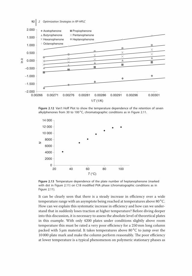
92 2 Optimization Strategies in RP-HPLC

−2.000

−1.500

−1.000

−0.500

0.000

0.500

1.000

1.500

2.000

0.00266 0.00271 0.00276 0.00281 0.00286 0.00291 0.00296 0.00301

ln k

1/T (1/K)

Acetophenone Propiophenone

Butyrophenone Pentanophenone

Hexanophenone Heptanophenone

Octanophenone

Figure 2.12 Van’t Hoff Plot to show the temperature dependence of the retention of sevenalkylphenones from 30 to 100 ∘C, chromatographic conditions as in Figure 2.11.

0

N

2000

4000

6000

8000

10 000

12 000

14 000

20 40 60

T (°C)

80 100

Figure 2.13 Temperature dependence of the plate number of heptanophenone (markedwith dot in Figure 2.11) on C18 modified PVA phase (chromatographic conditions as inFigure 2.11).

It can be clearly seen that there is a steady increase in efficiency over a widetemperature range with an asymptote being reached at temperatures above 80 ∘C.How can we explain this systematic increase in efficiency and how can we under-stand that in suddenly loses traction at higher temperature? Before diving deeperinto this discussion, it is necessary to assess the absolute level of theoretical platesin this example. With only 4200 plates under conditions slightly above roomtemperature this must be rated a very poor efficiency for a 250 mm long columnpacked with 5 μm material. It takes temperatures above 80 ∘C to jump over the10 000 plate mark and make the column perform reasonably. The poor efficiencyat lower temperature is a typical phenomenon on polymeric stationary phases as

2.3 Methodology of Optimization 93

they do not possess pore structures for unhindered and fast diffusion even forsmall molecule analytes. This leads to slower mass transport than silica-basedcolumns of a similar particle size. So it must be assumed that a significantlyhigher slope of the C-term in the van Deemter equation 2.8 is obtained. It haspreviously been derived from this equation that the C-term is controlled bythe diffusion coefficient. So the next logical step would be to discuss how thediffusion coefficient depends on temperature.

Equation 2.10, which is a simplified form of the Wilke–Chang equation [11],shows the relationship between temperature and diffusion. In this equation, 𝛹 is aconstant that depends both on the solvent and the analyte molecule. For those whoare interested in the quantitative relationship, the diffusion coefficient is inverselyproportional the molar volume to the power of 0.6, so approximately to the squareroute of molecular mass (depending on detailed molecular structure, in particularfor macromolecules). In this example, neither the solvent nor analyte is altered,and thus it can be directly concluded how the temperature influences the diffusion2.10. It shows the linear increase of Dm with increasing temperature, but at thesame time we have to consider the decrease in viscosity, which is also a functionof temperature, thus increasing the diffusion coefficient even more.

Dm(T) = 𝛹 •T

𝜂(T)(2.10)

The dependence of the viscosity is unfortunately not linear but rather exponen-tial and the curve is strongly dependent on the molecular properties of the solvent.The experimentally determined dependence over the span from 25 to 200 ∘C isshown in Figure 2.14 for three typical RP-HPLC solvents and one mixture of waterand acetonitrile. Water shows the strongest deviation from a linear relationshipand between 25 and 50 ∘C with the viscosity dropping by 40% relative to its originalvalue, but with the subsequent increase to 75 ∘C only further 20% decrease in the

400.0

0.2

0.4

0.6

η/η

25 °

C

0.8

1.0

60 80 100 120

Temperature (°C)

Water

Acetonitrile/water 20/80 v/v

Methanol

Acetonitrile

140 160 180 200 220

Figure 2.14 Dependence of the (dynamic) viscosity 𝜂 on temperature for three represen-tative HPLC solvents and one acetonitrile–water mixture. Curves show the progression asrelative values of 𝜂 related to the viscosity at 25 ∘C.

94 2 Optimization Strategies in RP-HPLC

viscosity is observed and by less than further 15% as the temperature is increasedto 100 ∘C. Above 125 ∘C, there is minimal effect in increasing the temperature.The two organic solvents acetonitrile and methanol show less curved but overallmuch weaker temperature dependency than water. Adding high water content toacetonitrile brings the curve closer to that of water, but still significantly differentwith an interesting observation occurring at extreme temperatures close to 200 ∘Cwhere the response curve crosses that obtained with 20% acetonitrile content.

It can be concluded from these curves and the considerations related to Eq. 2.10that the viscosity effect in a water–acetonitrile 20/80 v/v mixture increases thediffusion coefficient by a factor of 3.5 when going from 30 to 100 ∘C. In addi-tion to this phenomenon is a direct temperature effect on diffusion due to thehigher kinetic energy of the solvent molecules. It can be seen that the relation-ship is linear but it is important to consider the absolute temperature, which onlyincreases from 303 to 373 K (please note that temperature is always expressed indegree celsius, unless the context requires K). This factor of 1.23 can almost beneglected relative to the factor 3.5 resulting from the viscosity. Nevertheless, it canbe expected to observe more than a factor of 4 faster mass transport in this sce-nario. The example shown in Figure 2.11 uses a water–methanol 25/75 v/v mobilephase, which will create a viscosity curve relatively similar to that of methanol. Itcan be assumed that there is a viscosity decrease by more than a factor of 2, whichcombined with the direct temperature effect (1.23) represents a 2.5-fold increasein Dm over the given temperature range. The van Deemter equation predicts thatthe optimal linear velocity (minimum of the curve) linearly increases with Dm.At the same time, the slope of the C-term linearly decreases with Dm. Both ofthese observations are favorable for fast chromatography. The optimal resolutionis obtained at higher analysis speeds and there is only a much smaller efficiencyloss when increasing the linear velocity into the C-term. We have not recordedtemperature-dependent van Deemter curves for the application in Figure 2.11.Experimental van Deemter curves for pentylbenzene in a relatively viscous eluentrunning on a silica-based reversed phase are shown in Figure 2.15 for three differ-ent temperatures (25, 40, and 60 ∘C). The faster diffusion reduces the C-term inthis viscous eluent by a factor of almost 3 over the 35 ∘C temperature range andwith this factor the optimal linear velocity increases from 0.7 to 2 mm/s. By themathematical derivation of Eq. 2.8 for u, it is possible to determine that the min-imum of the curve is proportional to Dm/dp giving an important considerationfor optimization the speed of analysis. With organic-rich eluents the minimum ofthe van Deemter curve moves approximately linearly with temperature increases,with the minimum observed when the stationary phase particle is decreased tomoving to the right (see Eq. 2.10 and Figure 2.14).

This knowledge, allows the plate number curve in Figure 2.13 to be discussedwith a clearer understanding of what is happening. It is a reasonable conclusionthat increases in the diffusion coefficient will not just linearly grow up to 80 ∘Cand then stop as the temperature is further increased. Such strict proportionalitybetween Dm and N could only be expected in a certain range of the C-termregime. The van Deemter curve for heptanophenone on the polyvinyl alcohol

2.3 Methodology of Optimization 95

00

5

10

15

H (

μm)

u (mm/s)

20

25

30

25 °C

40 °C

60 °C

35

40

1 2 3 4 5 6 7 8

Figure 2.15 Van Deemter curves recorded at three different temperatures, column: Pron-toSIL KromaPlus C18 5 μm, 250 mm× 4.6 mm, eluent: EtOH/H2O 80 : 20 (v/v), analyte: pentyl-benzene.

(PVA) stationary phase is not known, but it is possible to calculate from the flowrate of 0.5 ml/min that the linear velocity is approximately 1.5 mm/s. For efficientsilica-based 5 μm stationary phases running with a viscous (water–methanol)eluent at room temperature, this should be close to the van Deemter minimumfor a small molecule. We already discussed that polymer-based stationary phasesoften suffer from slower mass transport due to their pore structure. The strongefficiency increase with increasing temperature leads to the conclusion thatu= 1.5 mm/s is already located far in the C-term, resulting in slow mass transporton the PVA material. If the conditions are chosen such that the dispersionprocesses are dominated by the C-term and the temperature is increased, themain effect that comes into play is the decreasing slope of the C-term resultingin efficiency increase. At the same time, the minimum of the curve moves tothe right, which can be considered as rolling down the C-term toward the curveminimum as a consequence. As soon as the curve minimum is approached, theefficiency increase will slow down and on increasing the temperature, will resultin the B-term becoming the dominant dispersion process, leading to an efficiencydrop with further temperature rises. This explains why the slope of the curve inFigure 2.13 flattens at 90 ∘C, and it can be concluded that it takes approximately100 ∘C to be at optimal efficiency with u= 1.5 ml/min on the PVA material. Sothe PVA needs this high temperature to enable chromatography with reasonablespeed, but fortunately this phase is stable at 100 ∘C, whereas most silica-basedphases would fail, even in the absence of buffers.

This discussion reveals a risk involved with temperature increase: for a methodthat is efficiency optimized at ambient temperature, but is used at increased tem-perature, the efficiency will drop because the B-term of the van Deemter curvecomes into play if the linear velocity is increased accordingly.

96 2 Optimization Strategies in RP-HPLC

The relationship between temperature and viscosity has been explicitly dis-cussed, and it was also briefly mentioned how the pressure change can be used asan indicator for the viscosity change. Now it is the time to treat this in quantitativeways, as pressure is always an important limiting factor in kinetic optimization ofHPLC. Equation 2.11 puts all pressure determining variables in context. Pressureincreases linearly with column length L and linear velocity u and is inverselyproportional to squared particle diameter (dp2). Pressure increases with theviscosity, which is a nonlinear function of temperature according to the curvesshown in Figure 2.14. For organic-rich eluents, the viscosity drops between 30and 80 ∘C approximately by 10% per 10 ∘C temperature increase. Hence, thecolumn head pressure under organic mobile phase content above 60% is at 80 ∘Conly about half that at ambient temperature.

Δp ∼ 𝜂•L•udp2 (2.11)

Decreasing the retention time is the first step in the speed-up of the separation.The related decrease in viscosity lowers the column pressure and allows for anincrease in linear velocity. It was mentioned above that this is actually necessary, toprevent longitudinal diffusion, B-term, processes becoming dominant and hencelosing separation efficiency. In the example of the alkylphenol separation, it canbe seen the potential reduction in analysis times related to a temperature increasefrom 30 to 80 ∘C with the following aspects:

1) The retention and thus analysis time reduces by a factor of 3, without a signif-icant change in resolution.

2) The column pressure at the same linear velocity is reduced by a factor of 2.3) Doubling the flow rate at the highest temperature, in order to generate the

original back pressure (260 bar), would allow for a sixfold reduction in analysistime.

This speed-up potential appears very appealing, and it raises the question whytemperature is not used to a much greater extent for expediting LC analyses.Wouldn’t it be a great alternative to the use of sub-2 μm particles that mostlyrequire UHPLC instrumentation to be able to perform at higher pressures? Threeimportant considerations have to be made to assess this, which will highlight thenegative aspects to this approach:

1) The preservation of the resolution is not guaranteed due to potential differ-ences in selectivity. In the given example, the experimental parameters arechosen such that the dispersion processes are dominated by the C-term, with astrong dependency between flow and the C-term, due to the slow mass trans-fer of the polymer material. Starting at the curve minimum, it would not bepossible to increase the chromatographic efficiency by increasing the tem-perature, not even with proper adaptation of u. In such a case, there wouldbe a high risk of losing resolution due to the lower retention (see Eq. 2.5 andFigure 2.2), and thus the faster method would possibly no longer meet therequirements.

2.3 Methodology of Optimization 97

2) It has been discussed in this section that temperature changes can stronglychange selectivity. It was shown in Figure 2.9 that these effects can evencause co-elution of compounds that are separated at a different temperature.Homologs are a case where the retention mechanism in RP-HPLC is asuniform as can be, which virtually excludes an influence of temperature onselectivity. Most analytical challenges, however, are more complex than this.

3) The endurance of stationary phases is always a strong function of tempera-ture though it depends on other operational parameters, too (see Chapter 4for more details). Kinetics of disintegration of the base material or the surfacemodification (bonding) simply follows the rules of chemical kinetics and socolumn deterioration is exponentially accelerated with temperature. Excellentstability for use at temperatures of 100∘ C and above can only be attributed tostationary phases based on organic polymers, porous graphite, and ceram-ics such as titania or zirconia (nonbonded). A few highly efficient silica-basedmaterials exhibit impressive stability at temperatures of 100 ∘C or more thanksto hybrid-silica and/or special bondings that protect the silica material. Nev-ertheless, the vast majority of silica-based RP-materials do not provide accept-able endurance at temperatures above 60 ∘C under common eluent composi-tions.

The three considerations above clearly show that the example of alkylphenoneson a polymer-based stationary phase show the limitations of this particular appli-cation. Nevertheless, the use of temperature to speed up separation is, in spiteof the discussed limitations, always worth a consideration. If method selectivityand the instrument capabilities allow for this, there are few reasons not to oper-ate at temperatures of about 50 ∘C to allow for the advantages of reduced analysistimes to be observed. To speed up a method by using elevated temperature, threeimportant considerations must be made:

1) The new method must still provide sufficient retention and resolution, so therules of k > 1 for the first eluting peak and Rs > 2 for critical pairs should stillapply.

2) For the modification of isocratic methods, the flow rate should be acceleratedin order to obtain the same column pressure as at the lower temperature. Asin the relevant temperature range, the diffusion coefficient changes approxi-mately with the same factor as the viscosity. Simultaneously, it allows for fullexploitation in the reduction in analysis times.

3) There are two more considerations for gradient methods. In order to respectthe gradient volume concept (see Chapter 3 and Section 2.3.4.1), the gradienttime must be shortened by the same factor as the flow rate is increased. Thehigher temperature will normally cause elution of the last eluting peak at anearlier position in the gradient. To exploit the full speed-up potential, the endof the gradient should be cut in order to place the last eluting peak back at theend of the gradient window.

With the information given in this section, separation scientists should feelforearmed to make proper use of temperature for both selectivity and speed

98 2 Optimization Strategies in RP-HPLC

optimization. The mobile phase composition in LC also has a similar effect tothe temperature. It influences both the mobile phase viscosity, with all respectiveconsequences and it also influences retention and potentially selectivity. This willbe addressed in the following section along with a perspective to what has alreadybeen discussed on temperature.

2.3.3The Value of Mobile Phase Composition versus Temperature in the Strive forOptimization in HPLC

The effect of eluent composition on the mobile phase viscosity was brieflyaddressed in the previous sections and Figure 2.14 clearly demonstrates this. Itwas mentioned that there are no simple linear relationships between viscosityand mixing ratio of solvents. The nonlinear effects are always related to theamount of heteromolecular interactions in the mixtures, which is a complex fieldhandled by thermodynamics of mixing. It is outside the scope of this textbookto treat it in a fundamental physicochemical way, but we discuss it empiricallyand point to all effects that are relevant for the LC user. It is a well-known factthat mixing of water and alcohols is an exothermic process, so the mixtureheats up when methanol is poured into a water containing flask. This occursbecause the intermolecular forces between methanol and water molecules areeven stronger than those between the molecules in the pure phases. This releasesenergy, facilitating the mixing process, but it also leads to a stronger associationof molecules in the mixed phase than in the pure phases. One consequence is thepronounced viscosity maximum that is observed in water–alcohol systems.

The experimentally determined dynamic viscosity 𝜂 is shown in Figure 2.16 forRP-HPLC relevant eluent mixtures. This also includes the quite uncommon mix-tures of water with alcohols other than methanol. All values are measured at 20 ∘C,while the relatively complicated temperature dependence was discussed in theprevious Section 2.3.2.2. It is important to note that the mixing ratio is given asmass-%. The advantage of mass-% is the absence of temperature influences dueto the different changes in solvent density with temperature. It is, therefore, amuch more precise practice to prepare mixtures for mobile phases gravimetricallythan volumetrically. The downside is that programming of mobile phase mixtureswith gradient instruments only allows control of volume-%. This has importantrelevance for the quantitative conclusions from Figure 2.16. Due to the lower den-sity of the organic solvents (methanol and acetonitrile <0.8 g/ml, while water has1.0 g/ml at ambient temperature), the maxima in the plot would move to the rightwhen transferring to volume-%. The shift is not linear, but increases with increas-ing organic content. While it changes the maximum for water–acetonitrile by lessthan 3% the water–methanol maximum is altered by almost 10% to the right andthus located at close to 50% methanol in volume.

While the curves in Figure 2.16 represent the situation at 20 ∘C, we can drawsimilar conclusions for the entire temperature range from 10 to 50 ∘C. The ampli-tudes of the curves are normally reduced with increasing temperature but the

2.3 Methodology of Optimization 99

Acetonitrile

Mass-% organic content

Methanol

Ethanol

Water

η b

ei 2

0 °

C (

cP

)

n-Propanol

3

4

2

1

3

4

2

1

0 20 40 60 80 100

Figure 2.16 Dynamic viscosity of mixtures of water with acetonitrile and different alcoholsat 20 ∘C. Please note that the x-axis is in mass-% rather than the more common volume-%.

maxima do not shift significantly in this temperature range. The following con-clusions are helpful in practice:

• With water–acetonitrile, it is observed that a viscosity maximum at 15% v/v,which is about 15% higher than the viscosity of pure water. The viscosity changesonly slightly between 0% and 30% v/v, but drops stronger at higher content andyields 40% of the viscosity of water in pure acetonitrile.

• With water–methanol, we observe a steeper increase striving toward the max-imum at 50% v/v, which is about 80% higher than the viscosity of pure water.The viscosity drops very strongly right of the maximum and reaches 60% of theviscosity of water in pure methanol.

• Mixtures of water with longer chain alcohols exhibit pronounced viscosity max-ima which is in the case of n-propanol more than a factor of 3 higher than theviscosity of pure water. Even pure n-propanol and ethanol show higher viscositythan water.

• The fact that water–methanol shows a 60% higher viscosity maximum makes itmuch less attractive than water–acetonitrile from a purely kinetic standpoint.The extremely high maxima of the longer chain alcohols virtually exclude themfrom standard application use (let alone the tax issue with ethanol). Never-theless, the positive impact of the different solvation properties of the alcoholmodifiers should never be underestimated for selectivity and peak shape opti-mization.

100 2 Optimization Strategies in RP-HPLC

We have seen in Section 2.3.2.2 with Eq. 2.11 that the column pressure isproportional to the eluent viscosity. Hence, the pressure with a 50% v/v methanoleluent would be almost twice as high as with acetonitrile at the same composition.The fact that the isoeluotropic composition of water–methanol is approximately5% higher, albeit helpful does not make a great difference here. Users of modernUHPLC instruments that provide up to almost four times the pressure capabilityof a conventional HPLC instrument may be inclined to just ignore this pressuredifference of factor 2. This should not be taken too easy though and to understandthis we need to look back into the Eqs. 2.8 and 2.10. We can derive that themolecular diffusivity depends on solvent viscosity. We have learned in the contextof temperature effects that solvent viscosity matters for the shape of the vanDeemter curve, both with respect to the position of the minimum and the steep-ness of the C-term. So we can directly conclude that the viscosity changes relatedto the eluent composition will change diffusion coefficients to a similar extentand have thus similar influences on the van Deemter curves. The van Deemtercurves for the same analyte and the same stationary phase used in Figure 2.15are shown for different mobile phase compositions but constant temperaturein Figure 2.17. Eluent composition was adapted respectively for isoeluotropicconditions to allow for a fair comparison. The viscosity of the water–methanoleluent is approximately twofold higher, while that of the water–ethanol eluent ismore than fourfold higher than with water–acetonitrile. We do not discuss thevan Deemter curves in a quantitative manner, as the scatter of the experimental

EtOH:H2O 80:20 (v/v)

MeOH:H2O 88:12 (v/v)

MeCN:H2O 85:15 (v/v)

u (mm/s)

H (

μm)

00

5

10

15

20

25

30

35

40

1 2 3 4 5 6 7 8

Figure 2.17 Van Deemter curves recorded at three different isoeluotropic eluent com-positions that differ markedly in viscosity, column: ProntoSIL KromaPlus C18 5 μm,250 mm× 4.6 mm, temperature: 25 ∘C, analyte: pentylbenzene.

2.3 Methodology of Optimization 101

data is relatively high, in particular for the water–ethanol system. Nevertheless,one can clearly see a massive impact of the solvent composition on the masstransfer (C-term), which is much higher (slower mass transfer) in the highviscosity compositions. Comparing the curves for acetonitrile and methanol,the rule of shifting the position of the curve minimum by the same factor as thediffusion coefficient (thus the same factor as viscosity and pressure) perfectlyapplies. The optimum linear velocity moves by factor 2 from 1 to 2 ml/min whenchanging from methanol to acetonitrile. This proves that there is more than thepressure limit of the instrument to take into account for the speed-up potentialof methods based on different eluents.

Δp ∼ 𝜂•L•udp2 Dm(T) = 𝛹 •

T𝜂(T)

umin ∼Dmdp

(2.12)

To express these relationships quantitatively, we have summarized all relevantequations introduced before as 2.12. These dependencies lead to the followingstatements:

• Doubling the viscosity 𝜂 doubles the column pressure Δp and reduces themolecular diffusivity Dm by half.

• To stick to the optimal linear velocity umin under this slower diffusivity, the flowrate F (and thus u) must be reduced by half as well.

• Having reduced the flow rate, the original column pressure will be observed,but simultaneously the analysis time has doubled.

Based on this we can draw two important conclusions:

1) With a given column type, temperature, and analyte, the minimum of the vanDeemter curve will always be at the same pressure level, no matter what themobile phase composition is, but the flow rate will have to be optimized indi-vidually.

2) As the mobile phase viscosity and the corresponding molecular diffusivitychanges during a gradient run, the constant flow mode is not the best optionfor efficiency optimization in gradient elution.

The second point leads to the conclusion that a pressure-constant modein HPLC, with the resulting flow gradients would be the optimal approachto gradient elution. These flow gradients could go over a wide range of up tothreefold changes when running from the maximum viscosity composition allthe way to the pure organic component (see viscosity changes in Figure 2.16).This pressure-constant mode would also improve the column lifetime, whichis reduced with the continuous pressure changes during gradient analysis. Atthe same time, the control of the gradient formation under constant pressure isa challenge, as the gradient slope would need continuous adaptation with thechanging flow rate in order to respect the gradient volume principle (Chapter3). This purely technical challenge can be solved through intelligent instrumentcontrol though. However, there is another important consequence of the constantpressure mode, as it removes the strict relationship between elution volumes and

102 2 Optimization Strategies in RP-HPLC

retention times that only exists in the flow-constant mode. This has implicationsfor the chromatographic behavior as the column ages. When the column perme-ability goes down over the lifetime of the column (it accounts for the resultingback pressure at constant flow), the retention times will change as a consequence,because the instrument control reduces the flow to keep the pressure constant.The only way to present chromatograms when operating in the pressure-constantmode consistently would be plotting the detector signal over the elution volumerather than over the retention time. This will not easily find acceptance in theuser community and is the most obvious reason why the pressure-constant modefor gradient elution has not yet gained ground.

The change of solvent composition as opposed to temperature change is animportant consideration to make in method optimization. It is important to over-see the kinetic consequences of both approaches beyond retention and selectivitywhen it comes to decisions. A practical challenge may be the decision whether toincrease temperature or content of the organic mobile phase when the goal is areduction of retention. To discuss this more quantitatively, we will learn anotherimportant rule of thumb:

Horvath rule for retention control in RP-HPLC: increasing the organic contentin the eluent by 1% has approximately the same effect as increasing the columntemperature by 5 ∘C.

This rule can be derived from the facts that

• 1% increase in methanol or acetonitrile decrease retention by 5–8%• an increase in temperature of 1 ∘C decreases retention by 1–2%.

It is very obvious from these relatively wide ranges that the Horvath rule canonly give rough guidance, but it is still very helpful for practical method devel-opment. It is crucial to note that both organic content and temperature changeretention exponentially based on the fundamentals of equilibrium thermodynam-ics. Together with the applicable ranges for temperature and solvent composition,this allows for some important general considerations:

• The accessible range of temperature variation on common LC columns (using acolumn thermostat that allows working at subambient temperature) is approxi-mately 10–50 ∘C. In this span, the retention factor can be changed by not muchmore than factor 2.

• Mobile phase composition on every RP column can be changed between 5% and100% and allows changes in retention by a factor of 5000–10 000. It is thus somuch more effective than temperature that both can hardly be compared.

• To reduce the retention by factor 2 can either be achieved by increasing thetemperature by 30–40 ∘C or increasing the organic content by approximately10%.

• A temperature increase of 30 ∘C will improve the speed-potential of a methodwith more than 90% water in the eluent by 50–80%. With more than 90%methanol or acetonitrile content this potential will only be 20–40%.

• The increase of 10% acetonitrile in the mobile phase will not remarkably influ-ence the speed-potential of the method as long as the initial content is below

2.3 Methodology of Optimization 103

25%. If the initial content is above 30% the speed-potential will increase byapproximately 10%.

• Thorough consideration is very relevant in methods using methanol. With morethan 55% initial methanol content the speed-potential at 10% higher methanolincreases by approximately 20%. If the initial methanol content is below 40%,however, the speed-potential is decreased by approximately 15% because of thestrongly increasing viscosity in this range.

There is no generally applicable rule whether mobile phase composition ortemperature is the better way to reduce retention from a kinetic point of view.The above-mentioned rules can give some guidance, but in practical methodoptimization it is more important how the selectivity of the method is affectedby either organic content or temperature change and how much the highertemperature affects column endurance with the given application. The pictureis clearer if the original method uses high water content (e.g., more than 80%).In this case, temperature is normally the better choice, if no other considerationspeaks against it. If the organic modifier is even methanol and the original methodhas more than 60% water in the mobile phase, there is a clear incentive to employa temperature increase. The increase of 10% methanol-content will reduce theanalysis speed by 10–20% which is not very appealing. This competes againstmore than 50% speed improvement related to 30 ∘C temperature increase. Ifcolumn stability and selectivity allow for it, it is very clear what the better choicefor water-rich methanol eluents is: temperature increase without a shadow of adoubt.

So we have seen how complex the influence of temperature in HPLC can be, butwe have learned so many helpful rules that the user should really apply tempera-ture effectively in method optimization. Especially the combination of tempera-ture and mobile phase composition may be an excellent way to optimize methods.Temperature should always be considered as an important method variable. Ifa method uses temperatures below 40 ∘C, the reason for this should always bechallenged. There are three important conclusions for this chapter that shouldtake away all myths and misconceptions about the use of temperature in methodspeed-up.

1) The fact that temperature increase reduces retention has nothing in commonwith temperature-based kinetic improvement or speed-up of separations. Therelated reduction of retention may even be a risk for the method robustnessor resolution. Retention in LC can be much more effectively reduced withmobile phase changes, and it is a purely thermodynamic consideration thathas no place in kinetic optimization.

2) Kinetic improvement is solely about the time needed to generate a certainnumber of theoretical plates. Plates per time depend on molecular diffusivity,which can directly be influenced by temperature, mainly through reductionof eluent viscosity. From this, we can conclude a maximum practical speed-up potential by temperature by factor of 2, as this is the accessible range toinfluence the diffusion coefficient in practice.

104 2 Optimization Strategies in RP-HPLC

3) The common assumption that temperature increase can generally replacepressure increase for method speed-up is simply wrong. We have learnedthat a proper method transfer to a higher temperature implies working at thesame pressure as with the original method. If a given column type requires fora given application a certain pressure to work in the van Deemter minimum,but the instrument is not capable to support this, it will not help to justincrease the temperature. While the lower viscosity will allow increasing thelinear velocity at the given pressure, the minimum of the van Deemter curvewill move by the same factor to right. There is no way to escape the B-termthat is not accompanied by pressure increase.

2.3.4Accelerating Separations through Efficiency Improvement of Stationary Phases

We have learned in the previous section that the often neglected increase in tem-perature has a fundamental potential for reducing analysis times, but we also iden-tified the limitations. Using equivalent plate number as a comparator, the use oftemperature cannot realistically reduce analysis times by more than a factor of 2.This section addresses the much more common approach to reducing analysistimes by improvements in the column performance. The theoretical foundationwill primarily be the dependence of the van Deemter curve shapes on the sta-tionary phase particle diameter dp. Later, we also briefly discuss the potential ofsuperficially porous and monolithic stationary phase materials.

2.3.4.1 Systematic Speed-Up by Optimization of Particle Diameter and Column LengthIn Sections 2.3.2.2 and 2.3.3, the influence of the diffusion coefficient on the shapeof van Deemter curves was explicitly discussed. This discussion is progressed todetermine the influence of the particle diameter and how it translates into prac-tical value for the user. It was seen in Section 2.2.2 that the particle diameter dphas an effect on the A-term and the C-term, with the C-term being related to dp2.This points to an even stronger influence on efficiency than that of the diffusioncoefficient, Dm. To discuss this, the response of the van Deemter curves to changesin dp will initially be simulated. This will require a simple transformation of Eq.2.8 into a generic form with dp as the only variable. A value of 1 is assigned tothe constants 𝜆 and 𝛾 . The mass transfer factor 𝜔 will be assigned the value of0.15 and Dm will be approximated with 0.003 mm2/s (3⋅10−5 cm2/s), which rep-resents a typical small molecule of 200–300 Da diffusing at ambient temperaturein a medium with viscosity of 1 cP. We have discussed that Dm can be decreasedby a factor of 2 by raising the temperature but this is not relevant for the relativecomparison of different particle diameters. After inserting the above-mentionedvalues for chromatography of a small molecule in aqueous-rich mobile phases atambient temperature into Eq. 2.8, the generic form of a van Deemter equation isobtained, as shown in the last term in 2.13. This equation was published by Halàszin 1975 [12], and it certainly contains empirical elements. The formula is set upvery conveniently, so that the user can insert the linear velocity u in millimeter

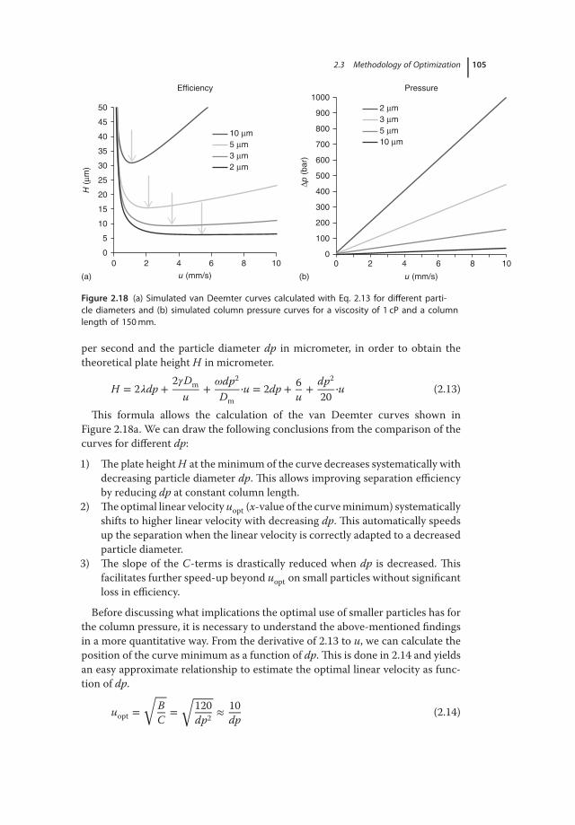
2.3 Methodology of Optimization 105

Pressure1000

10 μm

5 μm

3 μm

2 μm

700

800

900

500

600

400

300

200

100

00 2 4 6 8 10

(b)(a) u (mm/s)u (mm/s)

Δp (

bar)

0 2 4 6 8 10

50

Efficiency

0

5

10

15

20

25

30

35

40

45

H (

μm)

2 μm

3 μm

5 μm

10 μm

Figure 2.18 (a) Simulated van Deemter curves calculated with Eq. 2.13 for different parti-cle diameters and (b) simulated column pressure curves for a viscosity of 1 cP and a columnlength of 150 mm.

per second and the particle diameter dp in micrometer, in order to obtain thetheoretical plate height H in micrometer.

H = 2𝜆dp +2𝛾Dm

u+

𝜔dp2

Dm•u = 2dp + 6

u+

dp2

20•u (2.13)

This formula allows the calculation of the van Deemter curves shown inFigure 2.18a. We can draw the following conclusions from the comparison of thecurves for different dp:

1) The plate height H at the minimum of the curve decreases systematically withdecreasing particle diameter dp. This allows improving separation efficiencyby reducing dp at constant column length.

2) The optimal linear velocity uopt (x-value of the curve minimum) systematicallyshifts to higher linear velocity with decreasing dp. This automatically speedsup the separation when the linear velocity is correctly adapted to a decreasedparticle diameter.

3) The slope of the C-terms is drastically reduced when dp is decreased. Thisfacilitates further speed-up beyond uopt on small particles without significantloss in efficiency.

Before discussing what implications the optimal use of smaller particles has forthe column pressure, it is necessary to understand the above-mentioned findingsin a more quantitative way. From the derivative of 2.13 to u, we can calculate theposition of the curve minimum as a function of dp. This is done in 2.14 and yieldsan easy approximate relationship to estimate the optimal linear velocity as func-tion of dp.

uopt =√

BC

=√

120dp2 ≈ 10

dp(2.14)

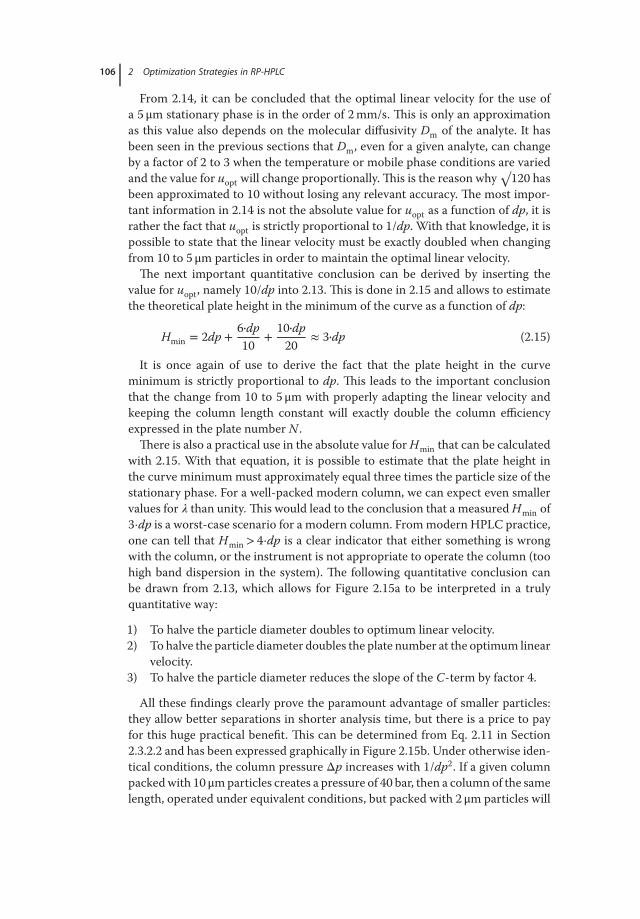
106 2 Optimization Strategies in RP-HPLC

From 2.14, it can be concluded that the optimal linear velocity for the use ofa 5 μm stationary phase is in the order of 2 mm/s. This is only an approximationas this value also depends on the molecular diffusivity Dm of the analyte. It hasbeen seen in the previous sections that Dm, even for a given analyte, can changeby a factor of 2 to 3 when the temperature or mobile phase conditions are variedand the value for uopt will change proportionally. This is the reason why

√120 has

been approximated to 10 without losing any relevant accuracy. The most impor-tant information in 2.14 is not the absolute value for uopt as a function of dp, it israther the fact that uopt is strictly proportional to 1/dp. With that knowledge, it ispossible to state that the linear velocity must be exactly doubled when changingfrom 10 to 5 μm particles in order to maintain the optimal linear velocity.

The next important quantitative conclusion can be derived by inserting thevalue for uopt, namely 10/dp into 2.13. This is done in 2.15 and allows to estimatethe theoretical plate height in the minimum of the curve as a function of dp:

Hmin = 2dp +6•dp10

+10•dp

20≈ 3•dp (2.15)

It is once again of use to derive the fact that the plate height in the curveminimum is strictly proportional to dp. This leads to the important conclusionthat the change from 10 to 5 μm with properly adapting the linear velocity andkeeping the column length constant will exactly double the column efficiencyexpressed in the plate number N .

There is also a practical use in the absolute value for Hmin that can be calculatedwith 2.15. With that equation, it is possible to estimate that the plate height inthe curve minimum must approximately equal three times the particle size of thestationary phase. For a well-packed modern column, we can expect even smallervalues for 𝜆 than unity. This would lead to the conclusion that a measured Hmin of3⋅dp is a worst-case scenario for a modern column. From modern HPLC practice,one can tell that Hmin > 4⋅dp is a clear indicator that either something is wrongwith the column, or the instrument is not appropriate to operate the column (toohigh band dispersion in the system). The following quantitative conclusion canbe drawn from 2.13, which allows for Figure 2.15a to be interpreted in a trulyquantitative way:

1) To halve the particle diameter doubles to optimum linear velocity.2) To halve the particle diameter doubles the plate number at the optimum linear

velocity.3) To halve the particle diameter reduces the slope of the C-term by factor 4.

All these findings clearly prove the paramount advantage of smaller particles:they allow better separations in shorter analysis time, but there is a price to payfor this huge practical benefit. This can be determined from Eq. 2.11 in Section2.3.2.2 and has been expressed graphically in Figure 2.15b. Under otherwise iden-tical conditions, the column pressure Δp increases with 1/dp2. If a given columnpacked with 10 μm particles creates a pressure of 40 bar, then a column of the samelength, operated under equivalent conditions, but packed with 2 μm particles will

2.3 Methodology of Optimization 107

generate 25 times this pressure, consequently 1000 bar. In addition to that effect ofdp on the column permeability, we must also consider the need to adapt u to main-tain the minimum of the van Deemter curve with the 2 μm column. It has beenseen that it is necessary to increase u by the same factor as dp is reduced, in thiscase a factor of 5. This would further increase the column pressure to 5000 barand directly raises the question, how is it feasible to work in practice with suchsmall particles at the optimum linear velocity. There must be something that hasnot been considered that needs to be incorporated into the discussion.

For the discussion of a method transfer to a column with a smaller particle size,a simple isocratic separation of uracil and five phenylalkanes will be considered.This separation will be optimized in two steps by changing the column and the lin-ear velocity twice until a significant speed optimization as shown in Figure 2.18 isachieved. The original separation was based on very traditional parameters, as thecolumn was a 10 μm material packed in a 250 mm column length and operated ata flow rate of 1 ml/min. The peak resolution was larger than required, so there wasno need to improve it. It can be seen that there is a systematic reduction in analysistimes by reducing the particle size and adapting the other parameters accordingly.This process requires that the equivalently bonded stationary phase material isavailable with other particle sizes packed in the respective column lengths. Thetwo simple rules to consider are as follows:

1) The column length L must be reduced by the same factor as the particle sizedp is decreased, so we keep the ratio L/dp constant. According to the funda-mental rules in chromatography presented in Section 2.2 this will keep theplate number N also constant, as long as the column with smaller particles isstill operated in the van Deemter minimum.

2) The linear velocity u must be increased by the same factor as dp is reducedin order to stick to the van Deemter minimum uopt. If the column diameter isnot varied, we will achieve this by increasing the flow rate F to the same factoras dp is decreased.

Following these two simple rules, it is possible to first reduce L from 250 to125 mm, as dp was reduced from 10 to 5 μm and simultaneously doubling F from1 to 2 ml/min. With these two changes, a fourfold increase in the analysis speedwas obtained, since a column of half the length, and with twice the linear velocityis being used. It is possible to go one step further by reducing dp to 3 μm andL accordingly to 75 mm (L/dp= const rule). Once again F needs to be correctedby the same factor to 3.33 ml/min and another almost threefold speed increase isobserved. Obviously, this optimization could have been achieved in just one stepgoing from the 10 μm particle column to a 3 μm particle and obtaining directly an11-fold (3.332) separation speed-up.

How does this parameter change then affect the column pressure Δp. Δpincreases inversely proportional to dp2; however, L and F , which affect the pres-sure, have also been simultaneously altered. To halve dp at otherwise constantconditions would result in a fourfold increase in Δp. The simultaneous halving ofL would result in a pressure increase at constant F of only twofold. However, as F

108 2 Optimization Strategies in RP-HPLC

is doubled to maintain the van Deemter minimum, the effective overall pressureincrease by systematically transferring a method to halve the original particle sizeis fourfold. In general, we find the following important relationship for analysisspeed and column pressure:

(1∕tanalysis) ∼ Δp (2.16)

The pressure will always increase by the same factor as the analysis speed. Wecan see this proven in the recorded pressure levels shown in Figure 2.19. Thespeed was overall increased 11-fold and so the pressure increased 11-fold from16 bar (rounded) to 175 bar. It is worth noting that this speed-up experimentwas carried out on a conventional HPLC instrument with nonoptimized fluidics.This can be concluded from the low back pressure of 16 bar with the originalmethod. A modern UHPLC would generate at F = 1 ml/min with the given eluentviscosity a pressure of 30–50 bar in the instrument alone without mounting acolumn. So the pressure resistance of a UHPLC instrument is two to three timeshigher than that of a 250 mm× 4.6 mm column packed with 10 μm particles. Itcan also be seen from the zoom into the chromatogram recorded on the short3 μm column that the early eluting peaks show a pronounced tailing. This is aconsequence of severe dispersion effects in the conventional HPLC instrumentthat is not appropriate to operate a 75 mm× 4.6 mm column packed with 3 μmparticles.

With the next example shown in Figure 2.20, the speed-up of a gradient sepa-ration performed on modern UHPLC-type columns and instrumentation is dis-cussed. The attempted use of a narrow bore (2.1 mm) column packed with 2.2 μmparticles requires an instrument with significantly reduced extra-column volume.This also includes the adaptation of the flow cell volume and the requirement offaster data handling by the detector electronics (which was already a prerequisitein the example in Figure 2.19). Moreover, the instrument must be able to handleprecise injection of 2 μl sample volume and withstand a column pressure of almost600 bar.

As well as the two rules discussed for the speed optimization of isocratic meth-ods, it is necessary to include another rule to allow for the correct optimizationof gradient programs. In order to make sure that the shorter and more efficientcolumn is not overloaded by volume and to achieve the same peak height in aconcentration proportional detector, it is necessary to include another rule in bothisocratic and gradient speed-up. If the column diameter is not changed during themethod change, these additional rules are as follows:

1) The gradient time tG must be shortened by the product of the flow increasefactor times the factor at which we reduced the column length. Thus,the following proportionality must be considered tG ∼ F ⋅ L which impliestG ∼ 1/dp2, respectively.

2) The injection volume V inj must be reduced by the product of columnreduction factor times the square root of the particle size reduction factor(V inj ∼

√dp ⋅ L).

2.3 Methodology of Optimization 109

250 × 4.6 mm, dp = 10 μm, F = 1 ml/min

Fourfold speed125 × 4.6 mm, dp = 5 μm, F = 2 ml/min

75 × 4.6 mm, dp = 3 μm, F = 3.3 ml/min

Δp = 16 bar

Δp = 61 bar

Δp = 175 barzoom

Uracil

Uracil

C1

C1C2

C3 C4 C5

0 1 2 3 4 5 6 7 8 9 10 11 12 13 14 15

0 1 2 3 4 5 6 7 8

Time (min)

9 10 11 12 13 14 15

0 1 2 3 4 5 6 7 8 9 10 11 12 13 14 15

C2

C3 C4 C5

11-fold speed

Figure 2.19 Example for a systematicmethod speed-up by optimization of particlediameter dp and column length L. Sample:uracil und phenylalkanes C1 –C5; station-

ary phase: Prontosil 120-C18-AQ (Bischoff),mobile phase: 80/20 (v/v) ACN/H2O, temper-ature: 20∘C; L/dp= 25. All other conditions asshown in the figure.

For the example presented in Figure 2.20, it is necessary to shorten the tG by afactor of 2.8 for the first optimization step and by a factor of 6.2 for both steps intotal. It can be seen that the duration of the gradient time also corresponds to thereduction in analysis time. If tG is not altered in a gradient method and only thetwo rules for isocratic optimization are considered, the analysis time will not bemarkedly reduced and the chromatogram will look different.

For the injection volume, V inj, it is necessary to consider the changes in L and dpaccording to the above-mentioned rule. This implies a reduction factor of 2 for thefirst step and a volume reduction of 4 overall. In this case, all parameter changeshave been rounded (L, F , tG, and V inj) and for the second optimization step itis assumed dp= 2 μm instead of 2.2 μm. This was done to facilitate the followingcalculation. It can be shown in practice that this minor change does not matter forthe look of the chromatogram; however, the speed-up factor was 20% higher thanit would have been with the correct calculation. The reason is that resolution ingradient methods is less influenced by the exact particle diameter than is the casein isocratic methods.

110 2 Optimization Strategies in RP-HPLC

Δp = 90 bar

Δp = 270 bar

Δp = 575 bar

2.8-fold speed

6.2-fold speed

0 1 2 3 4 5 6 7 8 9 10 11 12

Time (min)

250 mm × 2.1 mm, 5 μm

150 mm × 2.1 mm, 3 μm

100 mm × 2.1 mm, 2.2 μm

F = 0.30 ml/min

F = 0.50 ml/min

F = 0.75 ml/min

tG = 12 min

tG = 4.3 min

tG = 1.9 min

Vinj = 8 μl

Vinj = 4 μl

Vinj = 2 μl

Figure 2.20 Example for a systematicspeed-up of a gradient separation. Sample:parabens C1 –C4; stationary phase: Acclaim120-C18 (Thermo Scientific, Sunnyvale, USA),

gradient: from 60/40 to 20/80 (v/v) H2O/ACNwith the respective tG; temperature: 40∘C;L/dp= 50. All other conditions as shown inthe figure.

For the discussion on column pressure change, it is necessary to take intoaccount the pressure in a gradient method changes during the run. All pressurevalues given Figure 2.20 apply to the initial phase of the gradient where theviscosity is at the highest level. Looking at the figures, we could prove withthis second example the rule from 2.16 valid. This rule implies an importantconclusion for the speed potential of UHPLC in both gradient and isocraticmethods:

In a fair comparison based on equivalent resolution and by exploiting both thefull pressure capability of a 400 bar conventional HPLC system as well as that ofa 1200 bar UHPLC system, the analysis speed will be increased by not more thanfactor 3.

This finding may take away some of the magic of UHPLC, but in any case itinitiates the question what is behind the often reported speed-up factors of 10and more when going from HPLC to UHPLC. The two major reasons are thatthe HPLC is not used to the full pressure capabilities (which is often hamperedby system volume and detector influences as well), but mostly the fact that theresolution is reduced during the method speed-up (no proper method transfer).This is illustrated in the example given in Figure 2.20.

The fastest separation in Figure 2.20 is taken as a starting point for method opti-mization. The average resolution of Rs = 7 is much higher than required, whichallows the column length to be shortened, to 50 mm half of the original columnlength, L. The results obtained from the shorter column are shown in Figure 2.21.

2.3 Methodology of Optimization 111

6.2-fold speed

12.5-fold speed

Δp = 575 bar

Δp = 315 bar

25-fold speed

Δp = 626 bar

0.0 0.25 0.5 0.75 1.0 1.25 1.5 1.75 2.0

Time (min)

50 mm × 2.1 mm, 2.2 μm

F = 0.75 ml/min

tG = 0.95 min

Vinj = 1 μl

50 mm × 2.1 mm, 2.2 μm

F = 1.50 ml/min

tG = 0.48 min

Vinj = 1 μl

100 mm × 2.1 mm, 2.2 μm

F = 0.75 ml/min

tG = 1.9 min

Vinj = 2 μl

Figure 2.21 Further speed increase of the separation shown in Figure 2.20. A reduced reso-lution was tolerated here, as L/dp was reduced from 50 to 25.

The gradient time is reduced by half, following the rule mentioned previously(0.85 min instead of 1.9 min). The injection volume is also reduced to half of theoriginal value (1 μl instead of 2 μl). Comparing the upper two chromatograms inFigure 2.21, it can be observed that the pressure was reduced to the half, althoughthe separation is twice as fast. This means that there is a drop in the resolution,which goes with the square root of the column length, in this case the resolution isdecreased from 7 to 5, still much more than is required. The low pressure encour-ages a doubling in F and accordingly halving tG. The resulting chromatogram canbe seen at the bottom of Figure 2.21. Since the 2.2 μm particles exhibit a flat C-term, the resolution is still close to the value of 5. Comparing this chromatogramwith the original separation (upper chromatogram in Figure 2.20), it can be seenthat a sevenfold pressure increase (from 90 to 630 bar) gave us a 25-fold increase inanalysis speed. The run time was reduced from 12 min to half a minute. Neverthe-less, this is an unfair comparison and the result of a noncorrect method speed-up,as we reduced the resolution relative to the original chromatogram. In fact, most ofthese impressive speed-up factors often shown in marketing literature profit fromthe fact that the resolution in the original separation was way higher than needed.During the “optimization,” the method is not only accelerated, but resolution issacrificed by working on shorter columns, which gives rise to the much higherspeed increase than pressure increase. This example also demonstrates that a 12-fold speed increase with an allowed drop in resolution is easily achievable withinthe pressure range of a conventional HPLC instrument (middle chromatogram inFigure 2.21 running at only 315 bar). The essence of correct method acceleration in

112 2 Optimization Strategies in RP-HPLC

LC is to increase speed without changing resolution by running smaller particlesin shorter columns at higher linear velocity. Considering all the rules, the speedand the pressure are increased as a function of the squared particle diameter (dp2).Going from a 150 mm column packed with 5 μm particles to a 50 mm columnwith 1.7 μm and correctly adapting F by factor 3, would result in a ninefold speedincrease and ninefold pressure increase. The three times shorter column lengthalso allows a decrease in the solvent consumption by a factor of 3. If the columndiameter is also reduced, from 4.6 to 2.1 mm, another fivefold solvent saving isachieved. Hence, the overall solvent saving is by a factor of 15 and thus less than7% of the original mobile solvents are consumed.

All the rules and formula required for such a speed-up of a gradientmethod even with reduction of column diameter are summarized in thetables in Section 2.3.8.2. There are also web-based calculators that do allthe calculations automatically and the Thermo Scientific Chromeleon Chro-matography Data System even has such a calculator embedded in the methodeditor.

We have shown in Section 2.3.2.2 that analysis times can be reduced just basedon a temperature increase, which provides three clear advantages:

1) The need of a column with equivalent selectivity but smaller particle size andshorter length as a possible road block is removed.

2) Effort and cost to acquire such a column prior to starting the experiment isremoved.

3) The instrument does not have to support higher pressures.

These advantages are opposed by three important disadvantages of temperatureincrease:

1) Temperature increase only moves the minimum of the van Deemter curveto the right and flattens the C-term, but does not reduce the plate height atuopt. Hence, it does not enable to shorten the column length without reducingresolution and will thus only allow moderate speed-up factors up to 3, butnever a factor of 10.

2) The temperature change may result in selectivity change and will result inreduced retention. Therefore, the accelerated separation does not necessarilyfulfill the resolution requirements.

3) The increased temperature, in particular, with water-rich eluents at elevatedpH can deteriorate silica based columns relatively fast. So it often wouldeventually be cheaper to invest into a UHPLC column and run that at tem-peratures not higher than 40 ∘C.

A moderate temperature increase can provide a synergistic accompaniment toreduction in particle size to allow speed-up with transfer to a UHPLC-column. Thecombination of both (starting from a method that runs at ambient temperature)can yield speed-up factors of 20 instead of 10 with just reducing dp and L by afactor of 3.

2.3 Methodology of Optimization 113

2.3.4.2 Monoliths and Solid Core versus Fully Porous Phase MaterialsIt has been shown in the last section how small particles in shorter columnsallow systematic method speed-up. It has also been shown that the operatingpressure increases with the same factor as the reduction in analysis times. Whilethis appears to be a fair deal, having an understanding of the root cause mayenable the identification of even more favorable approaches to reducing analysistimes. Smaller particles provide lower dispersion due to the shorter pathwaysto circumvent them and to diffuse into their internal pore structure. Whenpacked into a dense structure they generate smaller flow-through channels. Withthese narrower channels, it is comparable to drinking through narrow straws asopposed to wide straws. It takes more suction effort to consume the same amountof beverage over time. The narrow channels generate a higher viscous frictionand the same applies in the packing of LC columns. Thus finding an approach tokeep the more efficient smaller particles at a larger distance from each other andconsequently increase the channel widths would have some benefits. This wouldcombine the incentive of small particles with that of large particles. Anotherobvious consideration is the search for larger particles with improved efficiencythanks to a different structure. Other alternative concepts are treated in moredepth in Chapter 4 with its focus on columns. These are columns based onmonolithic stationary phase structure as well as those packed from superficiallyporous particles that will be referred to as solid core materials for simplification.

Both concepts serve the demand of an improved efficiency to pressure ratio.While monolithic columns in spite of their continuous improvement over timestill lag behind on efficiency [13], we find that the solid core materials outperformclassical fully porous ones [14] of comparable particle size. Both concepts havetwo disadvantages though:

1) The choice of columns with different bondings and different base materials isstill much smaller than that of totally porous particle packed ones. In termsof monolithic columns, this applies even more to the number of differentmanufacturers.

2) The accessible stationary phase surface is smaller in relation to the columnvolumes, which results in a lower loading capacity and smaller retention fac-tors compared with fully porous materials with an equivalent diameter ofdiffusion pores.

These two disadvantages are less pronounced with solid core particles than withsilica-based monolithic phases. Moreover, the retention behavior of every mono-lithic column can be considered one of a kind given the manufacturing process forthe bonding. There are three more considerations with monolithic columns:

1) The structure-inherent higher total porosity (relatively wide channelsbetween the smaller size structure of stationary phase skeleton) leads to ahigher V M at given column size and thus to a higher solvent consumption.The higher permeability encourages increasing the flow rates and this con-sumes additional solvent during the injection process and the termination ofautomated analysis runs (delays from the data system).

114 2 Optimization Strategies in RP-HPLC

2) With concentration proportional detectors, the absolute peak area decreaseswith the same factor as the flow rate increases. This leads to smaller peak areasand since proper peak integration may always be a challenge, it can negativelyaffect quantification accuracy.

3) Even with the relatively powerful newer generation of silica-based monoliths,it is a fact that they still lag behind the efficiency (expressed as plate heightH) of modern sub-2 μm particulate stationary phases, while the recent smalldiameter solid-core particles outperform even the most efficient totallyporous particle phases.

With respect to a discussion of the practical value of alternative stationary phasearchitectures, we, therefore, restrict this section to the solid core approach.

Let us look at the method acceleration of a herbicide analysis that starts froma conventional method on a 250 mm column with totally porous 5 μm particles(similar to the example in Figure 2.20). In contrast to using a 2 μm totally porousmaterial in the last stage of the example in Figure 2.20, a 2.6 μm solid core sta-tionary phase with a similar selectivity will be used. If the 2.6 μm material had anefficiency which corresponded to its particle size and strictly following the rulesfrom Section 2.3.4.1, the new column length would need to be 130 mm in orderto achieve the same plate number. Since such a column length was not availableand instead two options were available, namely a 150 and 100 mm length column.In general, solid core particles provide better efficiency compared with their fullyporous counterparts, and so a 100 mm solid core column was chosen to progressthe method acceleration. With the assumption that the efficiency of this 2.6 μmsolid core material is 2.5-fold better than that of the original 5 μm material, it isalso necessary to accelerate the linear velocity by factor 2.5 to maintain the vanDeemter minimum. To reduce the amount of solvent consumption the columndiameter was reduced from 4.6 to 2.1 mm and due to the fivefold reduced crosssection resulted in a reduction in the flow rate of fivefold to achieve equivalentlinear velocity. Thus, for the method transfer initially the linear velocity should beincreased by a factor of 2.5 to account for the efficiency alterations, and then thelinear velocity is divided by a factor of 5 to adapt to the smaller column diame-ter. This results in a total flow rate conversion factor of 1∕2, resulting in the flowrate being reduced from 1 to 0.5 ml/min. Since the method applies gradient elu-tion, it was also necessary to alter tG. This must consider the reduction of thecolumn length and the increase of the linear velocity, so the factor is 2.52 = 6.3.The reduction of tG directly translates into the speed-up factor of the separation.The analysis time is eventually reduced by a factor of 6.3 from 16 to 2.6 min. Afterfinally adapting the injection volume and the detector settings, the method trans-fer is complete with the resulting chromatogram shown in Figure 2.22. A morethorough comparison between the two chromatograms will reveal that the ratioin retention time does not exactly follow the factor 6.3 for all peaks, but is formost peaks even smaller than 6. So the peaks do not exactly elute at the same gra-dient composition as this is a consequence of the not perfectly identical stationaryphase chemistry and the change in the total porosity 𝜀T of the column, a funda-mental challenge when changing between totally porous and solid core materials.

2.3 Methodology of Optimization 115

Rs = 2.51

Rs = 2.61

100 mm × 2.1 mm, 2.6 μm solid core

250 mm × 4.6 mm, 5 μm fully porous

F = 1.0 ml/min

F = 0.5 ml/min

tG = 2.6 min

tG = 16 min

Vinj = 1 μl

0 1 2 3 4 5 6 7 8

Time (min)

9 10 11 12 14 16

Vinj = 6 μl

6.3-fold speed

Δp = 375 bar

Δp = 105 bar

Figure 2.22 Speed-up of a gradient sepa-ration with transfer from the fully porousstationary phase Hypersil Gold (ThermoScientific, Runcorn, UK) to the solid corematerial Accucore RP-MS (Thermo Scien-tific, Runcorn, UK). Gradient from 65/35 to

40/60 (v/v) H2O/ACN in the respective tG;temperature: 30 ∘C; peaks in order of elution:tebuthiuron, metoxuron, monuron, chloro-toluron, diuron, linuron. All other conditionsas shown in the figure.

To assess the quality of the new method, the resolution for the critical pair wasanalyzed. In this case, the critical pair are the first two peaks: Tebuthiuron andMetoxuron. A drop in resolution from 2.62 to 2.52 was observed during methodoptimization; however, the new method still meets or even exceeds the regulatoryrequirements for resolution. It must be acknowledged that the chromatogram pat-tern and peak resolution could not be exactly transferred; however, a very similarseparation was achieved in only 16% of the analysis time and with 90% solventsavings.

The most interesting aspect of this method speed-up example is the changein column pressure though. In the original method, a pressure of 105 bar wasobserved at the start of the gradient. Following the rule shown in Eq. 2.16, it wouldbe expected to observe a 6.3-fold pressure increase associated with a respectivespeed increase. Actually, it can be seen in Figure 2.22 that the pressure increasedby less than a factor of 3.6–375 bar. Relative to the method transfer to a 2.2 μmtotally porous material with the same reduction in column length, more than 40%pressure increase has been saved. This proves the outstanding potential of thesesub-3 μm solid core materials. They allow for a sixfold speed increase accompaniedby a roughly threefold pressure increase, but without relevant loss in resolution.

Before closing this section, it is appropriate to give a short insight into the over-all market perspective of superficially porous or solid core materials. While therelated fundamental concept is as old as HPLC (Horvath reported in 1967 the useof surface etched glass beads for the first published HPLC separation [15]), theirbroad-based commercialization is relatively new and evolved predominantly over

116 2 Optimization Strategies in RP-HPLC

the past 10 years. In fact, the efficiencies associated with earlier versions were notvery good and so there was not much uptake of the technology. Meanwhile, thereare many different materials of this type available from a multitude of vendorsunder product brands such as Accucore (Thermo Scientific), Ascentis Express(Sigma Aldrich), Cortecs (Waters), Halo (Advanced Material Technologies),Kinetix (Phenomenex), Poroshell (Agilent), Raptor (Restek), or Titan (SigmaAldrich) just to list the most important brands in alphabetical order. While therange of selectivities still lags somewhat behind that offered with totally porousmaterials, there is now a decent choice of solid core-based different stationaryphases. It is also noteworthy that several solid core materials also exist nowadaysin a sub-2 μm format (Accucore Vanquish 1.5 μm, Cortecs 1.6 μm, Kinetix 1.3 and1.7 μm, Titan 1.9 μm). With these smaller particle diameter phases, the domain ofsolid core particle-based columns now surpasses the totally porous particle-basedcolumn on efficiency [16]. There is a trend observed that the efficiency advantageof solid core materials over fully porous ones of equivalent size decreases with theparticle diameter [17]. There is another potential advantage associated with theseparticles though, and this is their generally increased mechanical stability overtotally porous materials. Specifically, the use of particle diameter much lowerthan 2 μm when packed into columns of 100 mm or greater in length generatesan extreme pressures to achieve the van Deemter minimum. While the recentUHPLC instruments can go far beyond 1000 bar (currently up to 1500 bar), it isa challenge to manufacture stationary phases that provide acceptable enduranceunder such conditions. Here, the sub-2 μm solid core materials may be theformat of choice, but this is still an ongoing debate. Still under investigation isalso the fundamental understanding of the performance advantage of solid corematerials [14] and with that all the related quantitative predictions as a functionof particle size that would be very helpful to design parameter calculators formethod speed using solid core materials. We can expect more to come in thisfield.

2.3.5Optimizing Resolution by Particle Size and/or Column Length

We have seen with the speed-optimization in Section 2.3.4 that the particle sizedp is the predominant parameter to influence the plate number, N , being the pri-mary descriptor for efficiency to enable kinetic improvement of HPLC methods.Temperature can also change kinetic parameters in HPLC, but to a smaller extentthan particle size and it simultaneously changes thermodynamic parameters suchas retention and can sometimes even alter the selectivity. Kinetic optimization ismostly about increasing speed of analysis by providing a method that generatesthe same N in a shorter time. We now see how an increase of N through columnparameters can improve resolution and what considerations have to be made.

Understanding the influence of L, dp, and u on N and Δp gained from Section2.3.4.1, it becomes apparent that there are three different ways to increase the platenumber N together with the related implications:

2.3 Methodology of Optimization 117

1) Increase of the column length L which leads to equivalent increase in N . Asthe linear velocity u must be kept constant. Hence, the analysis time increaseswith the same factor as L.

2) Reducing the particle size dp, which leads to increase in N by the same fac-tor. At constant u an increase in Δp by the squared change of dp would beobserved. As we need to adapt u to the smaller Δp in order to stick to Hmin,we further increase the pressure, but also reduce the analysis time relative tothe original method.

3) A well-matched combination of reduction in dp and increase in L. In fact, itis this the only way to increase N without changing the analysis time, as theincreased L can be compensated by the increased u (provided availability ofthe required combination of L and dp).

The three options are discussed using example generated through numericalsimulations which generate the chromatograms presented in Figure 2.20. Thisfigure depicts a chromatogram with a peak triplet with a poor resolution of 0.94for both adjacent bands.

In Section 2.2.1, Eq. 2.5 that relates the resolution to the square root of the platenumber (RS ∼

√N) was discussed. This rule is instrumental for the prediction of

the resolution gain in the examples shown in Figure 2.23c and d. They all have incommon that the ratio of L/dp was increased from 20 to 50 relative to the originalmethod. So the resolution will increase by factor

√2.5= 1.58 from RS = 0.94 to 1.5.

In Figure 2.23b, this was achieved simply by increasing L from 100 to 250 mm. Thisresults in a relatively moderate pressure increase from 40 to 100 bar (the changein pressure being directly proportional to the change in column length, L). Simul-taneously the analysis time increased 2.5-fold and the related 1.58-fold dilution(peak volume grows with

√L) makes the peaks broader and lower in height. The

overall result is not very appealing, although we could achieve the target resolutionof 1.5. The chromatogram shown in Figure 2.23 appears much more appealing.Here, L is kept constant and dp was reduced 2.5-fold from 5 to 2 μm accompaniedby the required 2.5-fold flow rate increase from 1.5 to 3.75 ml/min. As a result ofthese changes, the target resolution was achieved in a fraction of the original anal-ysis time, but the price for this is a 15.6-fold pressure increase from 40 to 625 bar.As already mentioned, the simultaneous and matched change of L and dp is theonly way to achieve a resolution increase without changing the analysis time. Thisis shown in Figure 2.23d, which is obtained from the simulation using the practi-cally best possible scenario. Here, L was increased 1.5-fold from 100 to 150 mm,accompanied by a 1.67-fold decrease in dp from 5 to 3 μm. Hence, the increase inL approximately compensates for the required increase in u. The analysis time isonly increased by 10% here, but at the expense of a 6.9-fold pressure increase from40 to 275 bar (however, still in the range of a conventional HPLC instrument).

Next, the quantitative relationship between resolution and pressure will bereviewed but allowing for a fair comparison. Very simplistically, to achieve atwofold resolution increase it is necessary to increase L by factor 4. In order toperform the analysis in the same time, it is necessary to also increase F (ignoring

118 2 Optimization Strategies in RP-HPLC

Δp = 40 bar 100 mm × 4.6 mm, 5 μm

F = 1.5 ml/min

Rs = 0.94

L/dp = 20

250 mm × 4.6 mm, 5 μm

F = 1.50 ml/min

Rs = 1.5

L/dp = 50

100 mm × 4.6 mm, 2 μm

F = 3.75 ml/min

Rs = 1.5

L/dp = 50

150 mm × 4.6 mm, 3 μm

F = 2.5 ml/min

Rs = 1.5

L/dp = 50

Δp = 100 bar

Δp = 625 bar

Δp = 275 bar

(a)

(b)

(c)

(d)

Figure 2.23 Simulated chromatograms of anoriginal poorly resolving method (RS = 0.94)showing three different approaches toincrease the plate number by factor 2.5 andthus the resolution by factor 1.67. Note thatthe analysis time and column pressure dif-

fers significantly. The virtual mode of theChromeleon (Thermo Fisher Scientific, Ger-mering, Germany) UCI-50 A/D interface con-trol was used for the chromatogram simula-tion.

efficiency drop from a C-term effect) by factor 4. This modification results overallin a 16-fold pressure increase for kinetically doubling the resolution and withthe conclusion being that Δp increases with RS to the power of 4, as expressedin Eq. 2.17. Even when L, dp, and u are optimized to maintain the van Deemterminimum, Eq. 2.17 remains valid for resolution improvement at constant analysistime.

ΔRS ∼ Δp4 (2.17)

This finding is relatively sobering, but pressure capabilities of modern UHPLCinstruments do allow the user a greater leeway in resolution due to the extra pres-sure capacity. It is obvious that the use of sub-2 μm materials will provide evenhigher potential for resolution increase. Several constructed scenarios are com-pared in the next section (listed in Table 2.2) to demonstrate how this may appearin practice. u always has to be increased by the same factor as dp decreases tomaintain the optimum efficiency, which induces tremendous pressure increases.At constant column length the pressure increases with the third power of the

2.3 Methodology of Optimization 119

Table 2.2 Example for the attempt to improve resolution through efficiency increase whentransferring from HPLC to UHPLC. All numbers are theoretically modeled on the basis of theartificial method #1 (*method #2 is not feasible in practice).

Method dp (𝛍m) Lcolumn (mm) F (ml/min) N (plates) tanalysis (min) Rs 𝚫p (bar)

M1 5FullyPorous 100 0.25 6 000 10 1.0 100M2* 1.7FullyPorous 100 0.75 18 000 3.3 1.7 2 700M3 1.7FullyPorous 50 0.625 9 000 2 1.2 1 125M4 2.5SolidCore 250 0.625 ∼45 000 10 2.5 1 000M5 2.5SolidCore 150 0.625 ∼30 000 6.7 2.0 670

particle size reduction, while N and the analysis speed increase linearly. Someexample figures of obtained during such an optimization are shown as methodsM1 and M2 in Table 2.2. Starting with method M1 running on a typical conven-tional column generating a back pressure of 100 bar (for the sake of simplicity),an analysis time of 10 min and a resolution of Rs = 1.0, due to the poorly resolvedcritical peak pair. From method M2, it can be seen that maintaining a constantL, as the particle size is changed from a 5 to 1.7 μm yields threefold reduction inthe analysis time, 1.7-fold resolution boost (RS ∼

√N) but at the price of 27-fold

pressure increase. As the 2700 bar are in no way feasible on commercial instru-mentation, the only solution is to shorten L and slightly the decrease flow rate(M3). While this brings the pressure into a commercially viable operational range(∼1100 bar), the related plate number increase only translates into Rs = 1.2, stillinsufficient for practical requirements.

However, an alternative approach can be considered using superficially porousparticles (dp of 2.5 μm for simplicity) run at 2.5-fold higher u (or F) and the rea-sonable assumption that a similar efficiency increase as with changing to 1.7 μmtotally porous particles occurs. As optimizing the analysis time is not the goal,the column length is increased to 250 mm by the same factor as the eluent veloc-ity (this was practically impossible with the 1.7 μm material) was increased. Thecalculated result is shown as M4 and yields Rs = 2.5 (more than required) withthe same analysis time as method M1 and still at a practically very feasible Δpof 1000 bar. Moving on to M5 finally yields the perfect resolution (Rs = 2.0) com-bined with a 33% reduction in analysis time but still very much in the pressurecomfort zone of modern UHPLC instruments (670 bar). These observations allowfor three principal conclusions:

1) It is much more effective to increase selectivity for resolution improvementin LC, as was already concluded in Section 2.3.1.1.

2) If an increase in resolution and not a reduction in analysis time is the goal,then the focus should be on a moderate reduction in dp and use the requiredincrease of u to run a longer column at similar analysis time.

3) As superficially porous particles with diameters between 2.5 and 3 μm canprovide similar efficiencies to fully porous sub-2 μm ones, they may offer bestpotential for kinetic resolution boost (provided the selectivity fits).

120 2 Optimization Strategies in RP-HPLC

2.3.6High-Resolution 1D-LC and 2D-LC to Fully Exploit the Potential

The term high-resolution LC is not generally defined. It has been shown thatthe kinetic resolution potential of a chromatographic method correlates withthe square root of the achievable plate number for the given analytes. However,there may be different approaches on how to realize this resolution potential.When faced with the challenge of separating two compounds when no methodwith 𝛼 > 1.05 is available, it is necessary to have N > 20 000 to obtain the requiredRS. If selectivity is as low as 𝛼 = 1.02, then N ≈ 100 000 will be needed to gainan adequate separation. An example for an extreme scenario could be the chro-matographic separation of isotopes, where even 𝛼 ≈ 1.01 is difficult to achieve.Addressing such a challenge with several hundred thousand plates could be ajustification for ultra-high-resolution chromatography.

Much more common in the lab than those cases of two compounds that areextremely difficult to separate is the challenge of analyzing very complex mixtures.In such a complex mixture, it will be impossible to tune individual selectivities.These will be situations where a higher selectivity at a distinct part of the chro-matogram comes at the expense of another part of the chromatogram. This is aninherent issue if a high number of substances must be separated from a complexsample, because it is generally assumed that all parts of the separation space havean equal number of components. Any chromatographic method can be assessedfor a theoretical number of compounds it can separate in the best case. This is doneby the so-called theoretical peak capacity nC and considers perfectly equidistantpeaks at a resolution of 1.0 for all adjacent bands. It is the maximum number ofcompounds that can be separated by the respective method under these prerequi-sites. The theoretical peak capacity nC can be calculated based on chromatographyfundamentals that already have been introduced and is in general proportionalto

√N .

The peak capacity in isocratic separations nC,i is a function of the plate numberN and the retention factor of the last eluting peak ki, calculated according to 2.18:

nC,i = 1 + 14

•√

N • ln(1 + ki) (2.18)

The calculation of peak capacity in gradient elution nC,G is much more compli-cated and we do not derive the exact mathematical expression here. The relevanceof peak capacity in gradient is much higher though, since significantly better valuescan be achieved thanks to the fact that peak width does not increase significantlywith retention increase, as is the case in isocratic separations. For a good estima-tion of the peak capacity, Eq. 2.19 can be used:

nC,G ≈ 1 + 14

•√

N •10

1 + 10 tMtG

(2.19)

It becomes obvious that the relative gradient volume, the ratio of tM to tG, adoptsa similar role as ti in isocratic separations. From Eq. 2.18, it can be concludedthat the maximum achievable peak capacity in a reasonable analysis time using

2.3 Methodology of Optimization 121

isocratic elution is close to the square root of the plate number, N . This level isreached at ki = 50, while doubling the analysis time to ki = 100 will only increasenC,i by another 17%. This is much more favorable in gradient elution, where witha tG/tM = 50 an nC,G ≈ 2⋅

√N is achievable. Gradient elution also permits a peak

capacity corresponding to√

N at tG/tM = 7 to be achieved, which is seven times asfast at generating the same peak capacity as that obtained isocratically. Finally, itcan be concluded from Eq. 2.19 that even in very shallow gradients a peak capacityof 2.5⋅

√N cannot be practically exceeded. Finally, it can be concluded that about

160 000 theoretical plates are required to achieve a peak capacity of 1000 in anextremely shallow gradient (tG/tM > 1000). 160 000 plates are quite a challengeeven for UHPLC and the resulting analysis time from tG/tM > 1000 would not bevery appealing. Hence, even N = 250 000 is required to achieve nC = 1000 with areasonable gradient slope of tG/tM = 50.

As a take home message for estimation of peak capacity, we should rememberthe following:

1) The theoretical peak capacity is proportional to the square root of the platenumber oft he column in use.

2) In a tG/tM = 50 gradient method, it is necessary to have 2500 plates to achievenC = 100; 16 000 plates to achieve nC = 250, and 250 000 plates to achievenC = 1000.

2.3.6.1 The 2D-LC Approach to Increase Peak Capacities Beyond These LimitsA 150 mm long column packed with sub-2 μm particles will, even in the best case,generate no plate number larger than 40 000. Does this then mean that even mod-ern UHPLC cannot support peak capacities larger than 400? This is clearly notthe case but nevertheless it is important to investigate approaches to advance LCtoward such high peak capacities. A very effective way to boost peak capacity fur-ther is to add another dimension of separation, in other words to advance from1D-LC to 2D-LC. In the ideal case, the peak capacities of the two individual dimen-sions multiply for the total peak capacity of a 2D-LC method, following Eq. 2.20.

nC,2D-LC = 1nC•2nC (2.20)

This would imply that by simply combining two methods with nC = 100, a 2D-LC method with nC = 10 000 could be achieved. The practical implementation of2D-LC, however, is not a separation in true two-dimensional space, as is seenin gel electrophoresis or from a 2-step orthogonal development on a thin-layerchromatography plate. 2D-LC in practice is based on cutting fractions from theseparation in the first dimension and injecting them subsequently into a seconddimension. This can be done in a manual or automated way. In the automatedimplementation, one distinguished between the online and the offline variant. Theonline variant is characterized by parking the fraction in a loop, from which it isdirectly switched to a second dimension. In a standard type setup, this implies aperfect time match between cutting fractions from the first dimension and ana-lyzing them in the second. This challenge can be partially overcome by using a

122 2 Optimization Strategies in RP-HPLC

storage loop array for a higher number of fractions from the first dimension. In theoffline mode, the fractions are collected in vials and from them a certain aliquotis re-injected into the second dimension. Specialized autosamplers that can bothfractionate and reinject allow this fully automated without using an extra mod-ule. The application of such a setup for proteomics workflows is described in apaper from Eeltink et al. [18], which also presents peak capacity in comparison to1D-UHPLC methods. The instrumental prerequisites and also the commerciallyavailable solutions can fill a decent monograph, which is completely outside thescope of this chapter. Users who are interested in further details may refer to morespecialized textbooks [19].

What should be covered though are the prerequisites for the validity of Eq. 2.20.It is necessary to fulfill three important criteria to take full advantage of the peakcapacity from both dimensions:

1) The two combined methods must exhibit completely independent separationcriteria, or in other words they must have orthogonal selectivities.

2) The complete 2D retention space must be occupied, which means that thepeaks must spread from the lowest to the highest retention (in practice fromthe start to the end of the gradient) in both dimensions.

3) The number of fractions taken from the first dimension must reflect its sepa-ration performance adequately. The statistically required minimum oversam-pling equals two fractions per theoretical peak volume 4𝜎 according to theMurphy–Schure–Fowley rule. This implies a number of fractions that is twiceas high as the peak capacity of the first dimension.

An example for two automated offline 2D-LC method will now be reviewedand a discussion had on how well the three rules are respected in these examples.After that the challenges associated with translating theoretical peak capacity intopractical analytical value is discussed.

In Figure 2.24, a 2D retention map, as the chromatography softwareChromeleonTM (Thermo Scientific, Germering, Germany) displays it, is shown.The separation was done in the automated offline mode hence the fractionscut from the first dimension were collected in well plates and subsequentlyautomatically injected into the second dimension by the specialized fractioncollection autosampler. In the 2D retention map report view, the chromatogramsfrom the second dimension are vertically arranged from bottom to top andpositioned at the retention times on the x-axis that correspond to the time pointwhen the respective fraction collection was finished. To create the closed spotsfrom each peak, the software mirrors the chromatograms vertically and fills theresulting spots with color with an intensity proportional to the peak height. Thiscreates a similar picture as the protein scientists are familiar viewing with 2D gelelectrophoresis.

The 2D-separations will be analyzed and discussed further. The separationshown in Figure 2.24a combines a salt gradient-based SCX separation in thefirst dimension with a reversed-phase separation running at pH= 1.9 in aTFA-based water–acetonitrile gradient in the second dimension. The separation

2.3 Methodology of Optimization 123

E-coli pH 9.6 2D retention mapmin

min

9.0 12.0 14.0 16.0 18.0 21.025.0

30.0

35.0

40.0

45.0

50.0E-coli SCX 2D retention mapmin

3.0 10.0 15.0 19.025.0

30.0

35.0

40.0

45.0

50.0

min

RP x RPSCX x RP

1D SCX Method

2D

RP

pH

=1.9

Me

tho

d

1nc = 50

2n c

= 2

20

1D RP pH=9.6 Method(a)(b)

2D

RP

pH

=1.9

Me

tho

d

Figure 2.24 Automated off-line 2D-LC sep-aration of an Escherichia coli tryptic digest.Ten fractions of 1 min were collected fromfirst dimension. First dimension run on300 μm id, 150 mm length capillary columnsat 6 μl/min flow, second dimension run on75 μm id, 150 mm length nano columns at300 μl/min flow. SCX column was a PolySUL-FOETHYL Aspartamide 5 μm (PolyLC Inc.) run

in a phosphate buffer at pH= 3 with saltgradient up to 0.6 M NaCl in 15 min. All RPcolumns were Acclaim PA2 5 μm (ThermoScientific). First dimension RP was run atpH= 9.6 with triethylamine and gradient to50% acetonitrile in 15 min. Second dimen-sion RP (both methods) was run at pH= 1.9with TFA and gradient to 50% acetonitrile in30 min.

in Figure 2.24b combines a reversed-phase separation running at pH= 9.6 in atriethylamine modified water–acetonitrile gradient with the equivalent pH= 1.9RP separation from method (a) in the second dimension. Comparing the patterns,it can be seen that the peaks appear more or less statistically distributed in theSCX×RP method, as shown in Figure 2.24a. If the retention criteria of bothdimensions would be correlated, we would see the peaks arranged close to adiagonal line originating from the origin and with a gradient of 1. Looking at theRP×RP method shown in Figure 2.24b it can be seen that such a diagonal patternis present. This suggests that orthogonality is better fulfilled with the SCX×RPmethod than with the RP×RP, which is not surprising. The first prerequisiteappears well fulfilled with SCX×RP method shown in Figure 2.24a. The nextquestion addresses the coverage of the retention space in this method. The twoovals in Figure 2.24a demonstrate that there are spaces at bottom left, and evenmore pronounced at top right where hardly any peaks are located. From this, itmust be concluded that the second prerequisite is only partially fulfilled. Basedon the individual peak capacities (shown on the arrows in Figure 2.24a) andapplying Eq. 2.20, it would be expect a total peak capacity of 1nC = 50 times1nC = 220 resulting in 11 000 to be observed. The fact that the retention spaceis not fully covered will reduce this number. The third prerequisite, namely theproper oversampling from the first dimension will now be discussed in detail.For the SCX method a peak capacity of 1nC = 50 was calculated, so followingthe Murphy–Schure–Fowley rule it is necessary to transfer a minimum of 100fractions. This would imply cutting a fraction every 6 s and running subsequently

124 2 Optimization Strategies in RP-HPLC

100 separations with 30 min gradients. Taking the column re-equilibration ofanother 6 min into account, this would result in a total analysis time of 3600 min(60 h). Such conditions appear to be not very practical and mainly for this reasononly one fraction was collected every minute resulting in a total of 10 fractionsfrom the first dimension. This is by far insufficient to secure the theoreticalpeak capacity from the SCX separation. Following the Murphy–Schure–Fowleyrule, it can only be assumed, in a best-case scenario, an effective peak capacityequal to half the number of fractions, namely 5. So the maximum total peakcapacity considering 2nC = 220 from the second dimension would be 1100. Thisis only one-tenth of the nC,total = 11 000 value that we calculated based on fullyexploiting the first dimension and the complete retention space. The retentionspace coverage will be discussed later; however, initially important conclusionfrom the data and facts presented above can be made:

The theoretical peak capacity of the first dimension in a 2D-LC method (no mat-ter if performed online or offline) is relatively meaningless in practice.

To discuss this further, a scenario where equivalent peak capacity of nC = 100in both dimensions that would yield nC,total = 10 000 and under ideal conditions isdiscussed. Ideal conditions would imply transferring 200 fractions from the firstdimension, as has already been shown the Murphy–Schure–Fowley dictates thenumber of fractions is 2× 1nC. It will now be assumed that challenge to providea UHPLC method in the second dimension that can provide nC = 100 with totalcycle time (injection, separation, column re-equilibration in case of full gradients)of 4 min can be solved. Even if this is achieved, the total analysis time to run the200 fractions would sum up to 800 min (200× 4 min), thus more than 13 h. Whileit is obvious that the second dimension has to be fast, it is still much more ben-eficial to increase the peak capacity there, but reduce the number fraction fromthe first dimension. Especially with very steep gradients, where the cycle time isvery much influenced by column re-equilibration. Radically optimizing the sec-ond dimension for peak capacity per unit time can bring peak capacities in therange of nC = 200 in 6 min, when using a 150 mm column packed with a mate-rial that generates N = 50 000. This is an extreme challenge, but feasible today. Atpressures above 1200 bar and with use of increased temperature a V G/V M = 15 ispossible with such a column, which enables nC = 200 in 6 min. It is, therefore, pos-sible to generate nC,total = 10 000 with 1nC = 50 from the first dimension and thiswould need 600 min (100× 6 min) total analysis time. This is still 10 h, but a clearproductivity advantage over the approach with equivalent nC in both dimensions.

The practical implementation of faster 2D-LC methods builds on reducingthe number of fractions from the first dimension to a reasonable level of 30–50(yielding maximum effective peak capacity 1nC ≤ 25), and to further reduce theanalysis time in the second dimension by using, for example, very effective 30 mmsolid core columns or 50 mm second-generation silica monolith columns [20].These methods allow analysis times of less than 2 min per second dimensionrun, but only yield peak capacities below 100. Depending on how the firstdimension is implemented, the related 2D-LC methods can be run in a totalanalysis time of not more than 1 h, but would hardly exceed a total peak capacity

2.3 Methodology of Optimization 125

of 1000. If 50 fractions are run into a fast 2nC = 200 method, the total peakcapacity achievable in 5–6 h would be 4000, which can be considered a practicallimit for 2D-LC runs in acceptable analysis times. There are several differentapproaches to combining the gradients in the two dimensions and there is a wideperformance range that is spanned by the different ways to execute the seconddimension, which must also be matched to the molecular size of the analytes.An excellent overview on these possibilities is presented in a recent reviewarticle [21].

If the first dimension of 2D-LC method is radically under sampled, as is rela-tively common in offline 2D-LC methods, a consideration that differs markedlyfrom the commonly accepted way of assessing appropriate sampling rates can bemade. The separation in Figure 2.24a is discussed to exemplify this point. The givenSCX method generates peaks with a 𝜎t = 3 s, so one fraction of 1 min correspondsto 20× 𝜎t. The probability that the maximum of a randomly located peak zone inthis volume fraction is less than 1× 𝜎 away from the fraction start or end is lessthan 5% and this suggests that it is unlikely that a peak significantly smears overmore than one fraction. At such a degree of undersampling in the first dimension,it could be justified to consider the number of fractions equivalent to the effectivepeak capacity contribution from the first dimension. This approach would claim inno respect that the separation from the first dimension is appropriately reflected inthe graphical representation of the 2D chromatogram. It only claims that the prob-ability of a substance zone to significantly spread over two fractions is relativelylow. This consideration is also the foundation for the validity of the 2D retentionmaps shown in Figure 2.24 to graphically represent 2D-LC separations. They dis-play the zones from two different fractions as separated nonidentical compounds.At the given level of undersampling there is a sufficiently high probability that thisassumption is valid.

The discussion on how peak capacity can translate into practical value for theanalyst will now be reviewed. The examples shown in Figure 2.24 will again servefor that. The peak capacity contribution from the first dimension is now consid-ered to be equivalent to the number of fractions, so we assume 1nC = 10. Evenmore important is the fact that both the SCX method shown in Figure 2.24a andthe alkaline RP method shown in Figure 2.24b will contribute the same peak capac-ity of 1nC = 10, no matter whether their individual theoretical efficiencies differ.They are both limited by the same number of fractions and assuming they aresufficiently undersampled, considerate is reasonable to assume 1nC = nfractions. Asthe second dimension is identical in both methods, the outcome would be thatboth methods should provide a total peak capacity of 10× 220= 2200. The seconddimension nano-LC was run into an ion trap mass spectrometer, which allowsidentification of the respective peptides and construct the original proteins withthe help of appropriate software tools. The details on this are outside the scopeof this chapter, but typical workflows are common to proteomics experts. It isassumed that for the given discussion that the number of identified proteins is agood measure for the analytical value of both methods.

126 2 Optimization Strategies in RP-HPLC

SCX × RP RP × RP16% 51% 33%

Figure 2.25 Venn diagram to compare both2D-LC methods presented in Figure 2.24 withrespect to identified proteins. The percent-ages are calculated relative to the total num-

ber of identified proteins by combination ofboth methods, but not relative to the num-ber of proteins in E. coli.

The result of the method comparison regarding identified proteins is graphicallypresented in a Venn diagram shown in Figure 2.25. The RP×RP helped to find84% of the total number of identified proteins, while the SCX×RP method onlyenabled 67% to be identified. It is also noteworthy that 16% of all identified proteinscould solely be found with the apparently less powerful SCX-RP method. Thisshows that both methods were complementary to a certain extent. We now wantto characterize the two methods from Figure 2.24 in more detail. We already dis-cussed that the peak pattern in Figure 2.24a speaks for a more orthogonal methodthan the one in Figure 2.24b. Yet, was the RP×RP method (b) more successfulfor identification of Escherichia coli proteins. The next step is to determine theretention space coverage achieved in both separations. There are several methodspublished for its calculation [21] where the binning method according to Gilar [22]is a quite popular one. A very simplistic approach is applied, similar to the bin-ning method that accounts for the consideration of the 10 fractions from the firstdimension as 10 discrete spaces. The determination of retention space coveragewas simply done by measuring the length portion of signals above a certain thresh-old in each of the 10 individual traces. To achieve the total coverage for the entiremethod the average of these 10% was calculated. How this percentage space cov-erage can be envisioned is illustrated by the gray transparent shapes in Figure 2.24that surround the occupied spaces. The quantitative results yielded a surface cov-erage of 58% for the RP×RP method, but only 47% for the SCX×RP method. Ifthese coverage levels with the theoretical peak capacity of 2200 are multiplied forboth methods, it can be concluded that it is possible to have a practically effec-tive peak capacity of 1280 for the RP×RP method and an effective peak capacityof 1040 for the SCX×RP method. So the effective nC of method (b) is 24% higherthan that of method (a). Comparing the percentages of identified proteins, namely84% versus 67% it can be seen that the analytical success measured like this is 25%higher with method (b) than with method (a). Hence, it may be concluded thatthe retention space coverage correction is a meaningful way to determine effec-tively 2D-LC peak capacities that appear to translate systematically into analyticalvalue.

2.3 Methodology of Optimization 127

2.3.6.2 Boosting Peak Capacity in 1D-LC Further and How This Translates intoAnalytical ValueAfter the quite sobering conclusions from the previous section that it is difficultto generate really high peak capacities in 2D-LC within reasonable analysistimes, approaches to increasing the peak capacity in a single LC-dimensionbeyond nC = 500 (representing an approximate value to achieve on a 150 mmlong 1.7 μm column in gradient mode) will be considered. Peak capacities can beincreased by increasing plate numbers and plate numbers can be increased byextending column lengths. If longer columns packed with respective stationaryphases are not available, there is another approach that can be used to increaseL without changing the stationary phase. If a coupling device that generates nomeasurable additional band broadening is available, this can be used to simplycouple two or more columns in a similar fashion to a daisy chain. This also allowsa thermostatted separation path length of several times the maximum lengththat would generally fit into a column compartment. As has previously beendiscussed, extending L significantly will also lead to a pressure increase. So thequestion is whether these column lengths can still be operated in the van Deemterminimum using commercially available. This question will not be discussed ingreater detail in this chapter, but examples of using extreme separation pathlengths by coupling LC columns will be presented.

Initially, a 1000 bar instrument that can just handle methods above 800–900 barfor routine use, which means that it is not possible to run very long sub-2 μmcolumns. The first example to be reviewed will be based on a column chain offour 250 mm columns packed with 3 μm stationary phases, with L= 1000 mm andN ∼ 130 000, which was experimentally determined for this arrangement [23]. Itcan be calculated, with the help of Eq. 2.19, that with a gradient method, theoret-ical peak capacities of 800–900 could be achieved based on such a plate number.The resulting chromatogram obtained with such a daisy chain of four 250 mmcolumns packed with 3 μm material in shown in Figure 2.26. From the averagedbase widths of isolated peaks across the entire gradient a theoretical peak capac-ity of nC = 925 could be determined. This fully confirms the expectation basedon calculations from the plate number. The analysis time is significant though, asthe gradient volume required for this resolution (V G/V M = 35) results in a totalanalysis time of 5 h.

In the RP×RP separation shown in Figure 2.24, with proper consideration ofthe retention space coverage, an effective peak capacity of 1200 in an analysistime of 10 h could be achieved, which corresponds to a peak production rateof 2 peaks/min. The 1D-UHPLC chromatogram shown in Figure 2.26 withcomplete use of the retention space provides a 50% higher productivity of3 peaks/min. Moreover, the much higher instrumental effort to execute the2D-LC in Figure 2.24 must also be considered.

Similar to the attempt of significantly increasing the peak capacity per unit timein 2D-LC with a respectively productive UHPLC method in the second dimen-sion, boosting the effectiveness of 1D-UHPLC in order to separate such complexsamples faster, can also be considered. Knowing that today UHPLC instruments

128 2 Optimization Strategies in RP-HPLC

1000 mm × 3 mm, 3 μm

F = 0.5 ml/min

Δp = 780 bar

tG = 300 min

0 50 100 200 250 300

min

150

nc = 925

Figure 2.26 High resolution 1D-UHPLC sep-aration of a tryptic digest from a mixture offive proteins. A daisy chain of four 250 mmcolumns was coupled with zero dead vol-ume Viper couplers (Thermo Scientific, Ger-

mering, Germany). Stationary phase: Acclaim120 C18, 3 μm (Thermo Scientific, Sunnyvale,USA), temperature: 30 ∘C, tG = 300 min, nCcalculated from peak width of well resolvedpeptides.

can easily support 1200 bar methods, it is possible to increase the flow rate in themethod in Figure 2.25 to 0.75 ml/min (would correspond to 1200 bar) and shortenthe gradient time respectively to 200 min (tG/tM = 35, as before). The van Deemtercharacteristic of the material would easily allow for the resulting linear velocityand if everything scales according to the theory, the resulting productivity ratewould be 5 peaks/min. Nevertheless the experiment was not executed as the pres-sure of 1200 bar would have resulted in the Acclaim columns being operated faroutside of their pressure specification range.

It is very obvious that the elevated pressure capabilities of recent high endUHPLC instruments offer opportunities to achieve extremely high peak capac-ities in very reasonable analysis time. The question is what the right stationaryphase format would be to use with these instruments. One conclusion that canbe drawn with the help of kinetic plots is that higher pressure capabilities allowthe use of smaller particle sizes for extremely complex analyses. This is becausethese stationary phases can then be very effectively operated in longer columnsor column chains. An interesting particle size for such an attempt may be the2.2 μm format, which is in the middle between 3 μm and sub-2 μm phases withrespect to pressure permeability. At the same time, it can provide significantlyhigher efficiencies than 3 μm material. The approach of generating high peakcapacities very fast on 2.2 μm phases will be elucidated with the help of a naturalcompound analysis example, more specifically a Traditional Chinese Medicine(TCM) sample.

2.3 Methodology of Optimization 129

Similar to most natural products, TCM samples are normally very complexand can contain hundreds of compounds that are relevant for a screening assayto characterize them. Figure 2.27 demonstrates how the use of 2.2 μm particlescombined with extended column lengths can facilitate such challenging analy-ses. The original method on a 250 mm column with gradient duration of 18 minyielded a peak capacity of nC = 590 and created a pressure of 915 bar at the startof the gradient. To fully exploit the 1500 bar pressure capability of the VanquishUHPLC system, the column length was extended to 400 mm and the gradienttime, respectively, to 29 min. It was hoped that higher peak capacities could begenerated by better exploiting the pressure capabilities of the Vanquish UHPLCinstrument. The resulting pressure at the gradient start now increased to 1360 bar,but an impressive peak capacity of nC = 720 could be determined for this method.While nC = 720 may be considered not too impressive relative to the nC = 925shown with the method in Figure 2.26, it is worthwhile to note that the analysistime was reduced 10-fold from 300 to 30 min. If the production rate is calculated,24 peaks/min is achieved which is definitely a big improvement from all the meth-ods discussed earlier, regardless of whether 1D-LC or 2D-LC.

The observed increase in peak capacity of 22% matched the theoretical expecta-tion of a peak capacity increase with the square root of the column length exten-sion under respective gradient adaptation (

√(L2/L1)=

√(40/25)= 1.26≈ nC2/nC1

= 720/590= 1.22). A zoom into a particular part of the chromatogram shows howthe improved method provides better resolution (Figure 2.27). It can be seen howpeak 1 is split into two peaks and how some other peaks are getting sharper andresolution increases, while peaks 2 and 3 a actually lose resolution. It is impor-tant to be bale to characterize the overall benefit of the method with increasedpeak capacity and to identify an approach, which can be used to quantify the ben-efit in a screening method where peaks are not identified. Table 2.3 shows somefigures of merit to compare both methods. Under defined integration parame-ters, the overall number of peaks, as well the number of peak pairs with a certain

0min

2.6 3.1

4b

4a

3b3a

2

1

1a 1b

2

4.1 5.1

3a3b

4a

4b

min

mAUDAD: 280 nm DAD: 280 nm

L = 250 mm, tG

= 18 min

nc = 590, Δp

max = 915 bar

L = 400 mm, tG = 29 min

nc = 720, Δp

max = 1360 bar

mAU

18.5 0 30

Figure 2.27 Comparison of two genericexploratory methods for traditional Chinesemedicine (TCM) run a Vanquish UHPLC sys-tem (Thermo Scientific, Germering, Germany)with two different column lengths as spec-ified. Column id: 2.1 mm, L= 400 mm setup:

coupling 150 and 250 mm columns withViper coupling device (Thermo Scientific,Germering, Germany), gradient : from 0% to100% acetonitrile, flow rate: 670 μl/min, col-umn temperature: 45 ∘C.

130 2 Optimization Strategies in RP-HPLC

Table 2.3 Comparison between methods (a) and (b) from Figure 2.27 for number of identi-fied peaks and minimum level of resolution between all adjacent peak pairs as quality crite-ria to assess the value of different peak capacities.

Criterion nC = 590 method (a) nC = 720 method (b)

Total number of identified peaks 125 206Number of peaks with RS > 0.8 118 187Number of peaks with RS > 1.0 114 179Number of peaks with RS > 1.2 108 168Number of peaks with RS > 1.5 101 163

resolution is depicted. The number of identified peaks was more than 60% higheron the 400 mm column setup. Even more relevant are the statistics on the peakpair resolution. At all resolution levels the improved method provided more than50% additional peak pairs to meet this criterion. At the relevant RS = 1.5 level,the gain was even more than 50%. At least for this TCM example, the result is aclear demonstration of the practical value of nC to improve methods for complexsamples.

The following conclusions from the data presented here and from the findingsreported in more recent literature on highly optimized 2D-LC can be made:

1) With proper consideration of orthogonality, surface fractional coverage andoversampling of the first dimension, the maximum achievable practical peakcapacities in 2D-LC are in the ballpark of 3000–4000.

2) Even with speed optimized UHPLC methods in the second dimension, suchmethods take at least 4 h to run, which corresponds to a peak production rateof 10–15 peaks/min. Highly speed optimized 2D-LC methods for moderatepeak capacities of up to 1800 can nowadays be run in approximately 100 min,which corresponds to peak production rates of up to 18 peaks/min.

3) Using UHPLC pressure capabilities of 1400 bar allows the user to operate3 μm stationary phases in column chains up to 150 mm in length withV G/V M = 35 at reasonable analysis times of 4 h as well. This results in veryimpressive peak capacities for 1D-LC that can exceed nC = 1000, but onlymoderate peak production rates of 4–5 peaks/min.

4) With 1D-UHPLC pressures of 1400 bar it is possible to achieve the high-est productivity for complex sample analysis when using dp≈ 2.2 μm in400–500 mm column lengths. Such methods can achieve peak capacities of700–800 in only 30–40 min, which corresponds to amazing productivityrates of 20–25 peaks/min.

5) If peak capacities significantly higher than 1000 are required, 2D-LC is theonly option. For peak capacities of 500–700, 1D-UHPLC can provide excel-lent production rates and the effort of 2D-LC is difficult to justify, unless aspecific selectivity combination from the two dimensions proves indispens-able.

2.3 Methodology of Optimization 131

2.3.7Optimization of Limits of Detection and Quantification

In the introductory Section 2.1.3, it was discussed that an important aspectof optimization can be to improve a method for its applicability in traceanalysis. The nature of the mode of detection is very relevant in this case;whether the applied detector is concentration proportional like the verycommon UV detector or mass proportional like nebulizer-based detectors,for example, evaporative light scattering detector (ELSD) or charged aerosoldetector (CAD). This textbook contains dedicated chapters on nebulizer-basedor aerosol detectors (Chapter 10 on trends in detection), as well as for thecoupling of LC with mass spectrometry (Chapter 1). Here, the focus is onconcentration proportional detectors; UV detectors (VWD, DAD), fluorescencedetectors (FLD), electrochemical detectors (ECD), and refractive index (RI)detectors.

With concentration proportional detectors in particular, the difference betweenthe concentration-related and the absolute (mass- or amount-related) LOD andLOQ must be identified. This was already briefly discussed in Section 2.1.3, withthe following sections diving deeper into the details together with mathematicalcalculations. This will guide the practitioner to the optimization parameters andshould also take away some common misconceptions. The typical acronyms LODand LOQ will be used.

One of the simplest ways to determine both LOD and LOQ is based on theratio of the peak height to the noise in the chromatogram baseline, mostlycalled the signal-to-noise ratio (S/N). It is common practice to define the LODat S/N > 3. For the LOQ, the respective rule is S/N > 10. The LOD (and LOQ)of a method is thus low if the method shows a steep slope of the calibrationcurve combined with a low baseline noise. The slope of the calibration curveexpresses the change of detector signal as a function of change in analyteconcentration (or mass). This slope is defined as the so-called sensitivity of amethod, which is often confused with the LOD or trace detection performance.Both are related, but they are not identical and measured in different units.Since LOD and LOQ are strictly proportional, we only discuss LOD in thissection.

Both the sensitivity of a method and the LOD can be defined for the analyteconcentration or the absolute analyte mass (the amount injected onto the column).The concentration-related LOD cLOD can be calculated as follows:

cLOD =3•nbhp∕c

(2.21)

This calculation requires the baseline noise nb as well as the quotient of the peakheight hp and the analyte concentration c. The latter equals the slope of the cal-ibration curve for determination of analyte concentration in the sample by peakheight. The absolute (mass related) LOD mLOD is calculated similarly:

132 2 Optimization Strategies in RP-HPLC

mLOD =3•nb

hp∕minj(2.22)

Here, the quotient hp/minj equals the slope of the calibration curve for determina-tion of analyte mass in the sample by peak height. It is much more straightforwardto define mLOD for a method than to define cLOD, due to the impact of injec-tion volume size. This is shown with more detailed discussion and formula devia-tion in the following sections where the absolute detection limit mLOD is initiallydiscussed.

2.3.7.1 Absolute Detection Limit (Related to Analyte Mass on Column)The discussion is restricted in the section to UV absorbance detection. For this,we can use Beer’s law and calculate the peak height hp as follows:

hp =cmax•𝜀•d

MW(2.23)

In this formula, cmax is analyte concentration (mass per volume) at the maximumof the analyte band in the detector, 𝜀 the molar absorptivity (see Beer’s law), dthe optical path length in the detector flow cell, and MW the molecular mass ofthe analyte. It is possible to calculate the concentration at the peak summit in thedetector as follows:

cmax =minj•

√N√

2𝜋•VM•(1 + k)(2.24)

In this, we use the fundamental parameters of the kinetic and thermodynamic the-ory of chromatography plate number N , column hold-up volume V M, and reten-tion factor k. They all determine the peak volume, which is crucial for the concen-tration at the peak summit. Substituting Eq. 2.24 into 2.23, solving for hp/minj andeventually substituting this into 2.22 yields for the following equation to determinethe absolute LOD:

mLOD =3•nb

𝜀•d∕Mw•√

2𝜋•VM√

N(k + 1) (2.25)

This equation only applies for isocratic HPLC separations, as the parameters Nand k are not defined as such in gradient HPLC. This formula will be used to firstcalculate some representative values of mLOD in conventional HPLC and then forequivalent UHPLC scenarios. For both scenarios, the calculations are made fortwo different molar absorptivities 𝜀 and two retention factors k. The lower valueof 𝜀 represents an analyte with relatively poor UV detectability (e.g., acetic acidat 200 nm), the higher value reflects excellent UV detectability (e.g., chrysene at266 nm). The two retention factors 2 and 5 represent the typical working rangeobserved in isocratic HPLC separations.

For the conventional column, a 250 mm× 4.6 mm dimension packed with 5 μmat a total porosity of 𝜀T = 0.75 is used. This would typically result in V M = 3.1 mland N = 16 700 in the van Deemter minimum. A noise level of the conventional

2.3 Methodology of Optimization 133

Table 2.4 mLOD for an analyte of 300 Da in conventional HPLC using a 250 mm× 4.6 mm col-umn packed with 5 μm particles on a UV detector with 10 mm light path and 50𝜇AU base-line noise at different k and significantly different 𝜀.

Retention factor 𝜺= 100 l/mol⋅cm 𝜺= 100 000 l/mol⋅cm

k = 2 mLOD ≈ 80 ng mLOD ≈ 80 pgk = 5 mLOD ≈ 160 ng mLOD ≈ 160 pg

detector of 5⋅10−5 AU (50𝜇AU) is assumed, which is a realistic value for nb fora conventional HPLC detector. For the UHPLC scenario, a column with thedimension 100× 2.1 and densely packed with 1.7 μm particles at a total porosityof 𝜀T = 0.65 is used. This column will only yield a slightly higher efficiencyof N = 20 000, but a significantly lower hold-up volume V M = 0.225 ml. It isassumed that for a powerful modern light pipe detector optimized for sucha column format that nb = 10𝜇AU. Although very ambitious for a baseline inreal-life applications, this is possible after thorough optimization. For the sake ofsimplicity it will be assumed that a light path of 10 mm in both detectors exists.This is a reasonable assumption, as typical modern light pipe flow cells withextended flow path (e.g., 60 mm) are not compatible with such a column formatdue to mismatch between peak volume and flow cell volume. The molecular massof the analyte should be MW = 300 g/mol for both scenarios.

Equation 2.25 is used to calculate the mLOD values for the four representativeconventional HPLC scenarios, with results shown in Table 2.4. It can be seenthat the absolute LODs in conventional HPLC are in the order of 100 ng for ana-lytes with very poor absorptivity and 100 pg for analytes with excellent absorp-tivity. For typical aromatic compounds such as caffeine, a molar absorptivity of𝜀= 104 l/mol⋅cm is a reasonable estimate. LODs for those compounds in conven-tional HPLC would vary between 10 and 25 ng depending on the retention factor.

It is now interesting to see how much these absolute detection limits can bedecreased when transferring to a modern UHPLC method. The results of therespective calculations based on the given assumptions on the column formatand detector are represented in Table 2.5. It can be seen that the absolute LODscan be improved by a factor of approximately 80, suggesting that a factor of 100is a good estimate in general. Now the LODs for the compound with very poor 𝜀are in the single-digit nanogram range, for the analyte with excellent 𝜀 they arein the single-digit picogram range. The major contribution for these lower LODsstems from the increase of efficiency and column volume miniaturization.

The factor V M/√

N is 10- to 20-fold smaller in UHPLC than in conventionalHPLC. Based on the assumption made previously on the detector performance,the residual factor 5 came from the reduction of detector noise. If the conventionalmethod would be run on a top performing modern UHPLC light pipe detector, theabsolute LOD would only be factor 10–20 higher than that of the UHPLC methodon the same instrument.

134 2 Optimization Strategies in RP-HPLC

Table 2.5 mLOD for an analyte of 300 Da in modern UHPLC using a 100 mm× 2.1 mm col-umn packed with 1.7 μm particles on a UV detector with 10 mm light path and 10𝜇AUbaseline noise at different k and significantly different 𝜀.

Retention factor 𝜺= 100 l/mol⋅cm 𝜺= 100 000 l/mol⋅cm

k = 2 mLOD ≈ 1 ng mLOD ≈ 1 pgk = 5 mLOD ≈ 2 ng mLOD ≈ 2 pg

2.3.7.2 Concentration Detection LimitIt was shown in Section 2.3.7.1 that the absolute detection limit is a strict func-tion of the volume and efficiency of the separation column, as well as the responsefactor and baseline noise of the detector. To calculate the LOD in concentrationunits (cLOD), it was shown in Eq. 2.24 that the injected analyte mass minj must betaken into account. At a given analyte concentration in the sample, and in thiscase this relates to cLOD, minj can be varied, by changing the injection volume V inj.Thus, the concentration LOD can be lowered by just injecting a larger volume onthe column. Of course this is only valid as long as the increase of V inj does notsignificantly affect the resulting plate number N . At a certain V inj, however, oncethe column has become overloaded with the increasing sample volume, N startsto drop remarkably. It is possible to derive that the percentage of the V inj relativeto the resulting peak volume V peak from a given column actually equals the per-centage drop in N . So if V inj adopts 10% of the V peak, a column that could provide10 000 plates would only give 9000 plates. Tolerating a loss of 10% in N wouldresult in approximately 5% loss in resolution RS. While this is mostly tolerated, itwill be assumed as a general rule that only 5% loss in N resulting from the injec-tion variance is tolerable for optimal practical conditions. This would correspondto approximately 2.5% loss in RS. The loss factor is defined as 𝜃, and based on thatit is possible to formulate a general equation for calculating V inj from the columnparameters:

Vinj = 𝜃•Vpeak =𝜃•4•VM•(1 + k)√

N(2.26)

With Eq. 2.26 both the theoretical peak volumes V peak for representative conven-tional HPLC and UHPLC column formats as well as V inj at a given value of 𝜃(Table 2.6) can be calculated. The resulting injection volumes may appear rela-tively low, but they should be considered for making best use of the respectivecolumn efficiency. If a loss in N of 10% can be tolerated, one can inject twice thisvolume.

To derive a formula for the calculation of cLOD, it is necessary to divide Eq. 2.26by 2.25 and to obtain 2.27, which includes an approximate calculation for cLODbased on 𝜃 = 0.05:

cLOD =3•n0

𝜃•4•𝜀•d∕MW•√

2𝜋 ≈40•n0

𝜀•d∕MW(2.27)

2.3 Methodology of Optimization 135

Table 2.6 Peak volume and injection volume levels for representative column formats.

dp (μm) 5 3 2.2 1.7L (mm) 250 150 100 50dC (mm) 4.6 3.0 2.1 2.1V peak (at k = 2) (μl) 300 75 25 15V inj (at 𝜃 = 0.05) (μl) 15 4 1.25 0.75

The calculations assume H = 3⋅dp for all columns, 𝜀T = 0.75 for 5 and 3 μm columns and 𝜀T = 0.7for 2.2 and 1.7 μm columns.

One approximation is made in deriving this, namely that N does not changeat the V inj related to 𝜃 = 0.05, which appears to be fair given the considerationsabove. With the help of Eq. 2.27, cLOD can be calculated for a molecule with a MWof 300 Da and a 𝜀 of 10 000 l/mol⋅cm is in the range of 20 μg/l with a modern lightpipe detector and 100 μg/l on a more conventional detector. Interpreting Eq. 2.27further and comparing it to Eq. 2.25 the following very important conclusions fortrace analysis can be made:

1) The concentration related LOD (cLOD) is independent of the column volumeand column efficiency as long the injection volume V inj is properly adaptedto the respective column. Hence, cLOD cannot be improved by the columnparameters, as long as sufficient sample is available to apply the required V injfor optimum column load.

2) Provided sufficient sample, cLOD for a given analyte at the optimal detectionwavelength can only be influenced by the detection path length d and thebaseline noise nb with the given method and detector settings. Modern lightpipe detectors with more than 50 mm light path and low noise levels enable a10–20-fold lower detection limit than conventional detectors, but normallytolerate no peak volumes smaller than 100 μl without loss in resolution.

3) A reduction in column dimension and an increase in column efficiency cansolely improve the absolute detection limit mLOD. This can be very relevant ifthe sample size is limited though and it was the key incentive to develop nano-and capillary-HPLC for certain application fields like proteomics.

2.3.8Practical Guide for Optimization

2.3.8.1 General Optimization Workflow and Important Considerations and PrecautionsBefore a method can be optimized, there must be a respective method availableas a starting point. It was not the goal of this chapter to provide guidance forfundamental method development from the scratch, but to develop an existingmethod. Prior to starting method optimization, the user must become clear on thepossible deficiencies of the current method and identify its relevant optimizationpotentials in terms of parameters like, for example, resolution, speed, or detectionlimits. Once a deficiency is identified, the user must also analyze the method forthe root cause for these deficiencies. If a method shows insufficient resolution for a

136 2 Optimization Strategies in RP-HPLC

critical peak pair, the next step is to analyze retention factors, selectivity and platenumbers as well as peak asymmetries of the respective peaks to draw the properconclusions. This analysis will quickly show if the required minimum retention ofk = 1 is fulfilled (or if the peaks actually elute during the gradient), if no peak asym-metry is higher than 1.5 and if the plate numbers meet those of the column testprotocol (at comparable retention factors). Poor peak shapes should be addressedby verifying the state of the column with a standard test, too low retention may beaddressed by decreasing the solvent strength of the mobile phase or lowering thestarting composition of a gradient. However, it is often the selectivity that is theroot cause of insufficient resolution. This has to be empirically optimized startingfrom a change in the eluting conditions. This can be either a change of the organicmodifier under more or less isoeluotropic conditions, or potentially slight temper-ature or pH-variations. Another option is the change to a different column withideally orthogonal selectivity. If such a column is available, it is a quick test, if ithas to be purchased, one should start with variation of eluting conditions. Severalrules for a systematic procedure have been developed with valuable hints on therelated decision criteria discussed in detailed. A greater understanding of theserules is given in Chapters 3 and 4 of this text book.

In subsequent optimization steps the analysis time may be reduced. The firstapproach to reducing the analysis time should be a stepwise increase in the flowrate, possibly coupled with a temperature increase. In gradient methods, the gra-dient time must be reduced by the same factor as the flow rate is increased. Loss ofresolution or if a lower resolution does not meet the method requirements can bequickly seen as the flow is increased or if there is a matched increase of the flowand temperature (considering constant pressure). If such problems are encoun-tered, the next approach to reducing the analysis time should be to change to ashorter column with smaller particles respecting the L/dp= const rule. If the flowrate and gradient time (if applicable) are adapted according to the rules, this willbe a guaranteed success, provided the selectivity of the new column does not sig-nificantly deviate. If the original method provides relatively high resolution for thecritical pair (RS > 2.0), it will tolerate deviations in selectivity as well as flow andtemperature increases, or even a reduction of L/dp much more readily.

It is always highly recommended to verify the robustness of the optimizedmethod before implementing it in routine. If no elution parameter other thanflow rate was changed and the column is still well in the specified operatingpressure range, a thorough evaluation of peak resolution should be sufficient. Ifthe temperature was increased beyond 40 ∘C, the new method should be verifiedfor column stability by injecting 100–200 samples with no relevant changebeing observed in retention or efficiency. If mobile phase composition, pH ortemperature were varied, robustness of the new method must be proven withsingle parameter variation of the variable that was altered.

2.3.8.2 Overview on Valuable Rules and FormulaThis section will give a brief summary on all the relevant rules and formula thatapply in method optimization. They help to make estimations and give guidance

2.4 Outlook 137

to avoid critical failures. Wherever applicable, it also provides simplified approx-imations for calculations. In Table 2.7 the relevant information on instrumentalconsiderations can be found. The reader should also consider Section 1.2 in thiscontext, as it contains very useful information that can be readily applied beyondthe application of instruments in LC/MS. The following tables lead to methodrelated optimization criteria. This will address the separation column (Table 2.8),the analysis speed (Table 2.9), the retention in RP chromatography (Table 2.10),the resolution (Table 2.11), and also the peak capacity (Table 2.12). The formularelated to LOD have been developed and discussed in Section 2.3.7 and will notbe repeated here.

The following rules and formula cannot be complete, but they provide a concisesummary of all relevant information in this chapter and they can be used for arepetition as well as a general reference work.

2.4Outlook

It has been shown in this chapter how modern UHPLC with pressures up to1500 bar and optimized use of particle sizes slightly above 2 μm can achievetheoretical peak capacities of almost 1000 in less than 1 h. It is also possible toperform relatively demanding separations in about 1 min on sub-2 μm, ideallyusing solid core based short columns. Selectivity continues to be the mostimportant parameter in LC when in comes to resolution optimization. Thisis the incentive for column manufacturers to continuously develop materialswith new selectivities for relevant and challenging applications. At the sametime there is a trend toward solving as many applications as possible on a smallnumber of different columns, ideally only one. This is facilitated through thehigh plate numbers that UHPLC columns can generate in relatively short times.Since selectivity is still indispensable there is also desire for phases that allow forsignificant changes of selectivities by altering the elution conditions. Mixed modeor multi mode phases have a high potential for such a tuning via pH, ion strengthand organic modifier, while the temperature is not yet widely used as an additionalparameter. Alternatively, there is still significant improvement potential for thekinetic performance of such phases. Most of them do not exist in particle sizesbelow 3 μm, they are often not compatible with higher pressures, and peaksymmetries are sometimes not comparable to the quality obtained with modernC18 phases of equivalent particle size. There are two fundamentally oppositionaltrends observed. One is the increasing number of columns customized for certainapplications, for example, distinct biopharma characterization workflows, theother trend is striving for generic methods to solve as many analytical problemsas possible without any method development on just one column. While the newgeneric approaches are driven by the kinetic potential of modern UHPLC oftenin combination with fast and powerful mass spectrometry, specialty phases forcertain applications hardly take advantage of the kinetic capabilities of UHPLCand there is still discussion to determine if there is a need for these types of phases.

138 2 Optimization Strategies in RP-HPLC

Table 2.7 Instrument related volumes and detector settings.

Parameter Formula Approximations/rules

Comments

Gradient delayvolume (Gradientdwell volume)

GDVsystem =GDVpump+GDVsampler +V capillary(pump-sampler) +V capillary(sampler−column)

GDVHPG ≈V Mixer HPG: High pressuregradient pump(binary gradientpump)

GDVsampler ≈V loop + 5 μl

LGP: Low pressuregradient pump(quaternary gradientpump)

V cap(100 μm)≈ 0.08 μl/cm

LPG: Consider theGDV specified by themanufacturer orbetter determine ityourself (Dolan-Test)

V cap(130 μm) ≈ 0.1 μl/cmV cap(180 μm) ≈ 0.3 μl/cmV cap(250 μm) ≈ 0.5 μl/cm

Rules:Ideal:• GDVsystem ≤V M/2

Fair:• GDVSystem ≈V M

Maximum tolerable:• GDVsystem ≈ 2 ⋅V M

V M = column hold-upvolume (siehe “column”)

2.4 Outlook 139

Table 2.7 (continued)

Parameter Formula Approximations/rules

Comments

Volumes ofconnection tubings

No exact formula Rules:Ideal:• V tubings ≤V peak/5

Maximum tolerable:• V tubings ≤V peak

See above for estimationof tubings volumes fordifferent capillary IDsV peak =Peak volume(see “column”)

• Keep allconnections asshort as possible

• Keep tubing IDas low aspossible, inparticularbehind thecolumn

• Instrumentswith maximum600 bar pressurelimit: CapillaryIDs≥ 130 μm toavoid overpressure

Detector flow cellvolume

No exact formula Rules: • V cell is the lightirradiatedvolume in theflow cell

• Challengemanufacturerspecifications asnot all list theirradiatedvolume

• For banddispersionconsider also thevolume of heatexchanger infront of the flowcell

Ideal:• V cell <V peak/10

Maximum tolerable:• V cell ≈V peak/3

See “column” für V peak

(continued overleaf )

140 2 Optimization Strategies in RP-HPLC

Table 2.7 (continued)

Parameter Formula Approximations/rules

Comments

Data collection ratein detector (f det)

fdet ≥25√16⋅H

L

⋅ 1∕tR Approximation:fdet ≈

6⋅√

NtR

with N fromcolumn test protocol

• Formula appliesfor 25 datapoints at thepeak base wb(4𝜎t)

• Corresponds to30–40 datapoints within theintegrationlimits

• Is valid forisocratic analysisand shouldconsider tR ofmost earlyeluting peak

• For gradientmethods replacetR by tM

Alternatively: insert Hin exact formula as 3⋅dp

Time constant ofdetector (tC)

tC ≤ 0.1 ⋅√

16⋅HL ⋅ tR Approximation:

tC ≈ tR2⋅√

Nwith N from

column test protocol

• The inverse datarate is also agood estimationfor tC

• If the detectorsettings require“rise time” order“response time”instead of “timeconstant” applytwice the value

• For gradientmethods replacetR by tM

Alternatively: insert Hin exact formula as 3⋅dp

2.4 Outlook 141

Table 2.8 Columns, particle sizes and their operational conditions.

Parameter Formula Approximations/rules

Comments

Columnhold-upvolume V M

VM = L•d2

C4

•𝜋•𝜀T Approximation:VM ≈ L•dC•dC

2• Insert L and dC in mm

to obtain V M inmicroliter

• Approximation uses𝜀T = 0.63, a goodapproximation forUHPLC columns withtotally porous particles(conventional columnswill have up to 25%higher V M, solid corecolumns up to 25%lower)

Theoreticalpeak volumeV peak

Vpeak =√H•L•d2

C•𝜋•𝜀T•(1 + k)

Approximation:Vpeak ≈ 10•VM√

N

• V peak is defined as thepeak volume at thepeak base wb (4𝜎), thevolume within theintegration limits is20–50% higher

• V P can also bedetermined from thechromatogram bycalculating wb⋅F

• IfV peak real ≫V peak theoret.the correct detectorsetting must bechecked

Calculate V M withapproximationaboveAlternatively: insertH in exact formulaas 3⋅dp

(continued overleaf )

142 2 Optimization Strategies in RP-HPLC

Table 2.8 (continued)

Parameter Formula Approximations/rules

Comments

Optimum flowrate F

No general exactformula (depends onanalyte, mobilephase, andtemperature)

Approximation:Fopt ≈

dC•dC3•dp

• Exact determinationalways requiresmeasuring a vanDeemter curve

• Approximation validfor totally porousmaterial

• For solid corematerials assume50% higher value(20% for sub-2 μm)

Insert dC in millimeterand dp in micrometer, Fresults in milliliter perminutes

Linear velocity u(conversion fromflow rate)

u = 4•Fd2

C•𝜋•𝜀TApproximation:u ≈ 30•F

dC•dC

• For a totally porousmaterial uopt forsmall molecules isapproximately 10/dp

• For a sub-3 μm solidcore material uoptfor small moleculesis approximately15/dp

Insert F in milliliter perminutes and dC inmillimeter to obtain uin millimeter per second

2.4 Outlook 143

Table 2.9 Method speed-up.

Parameter Formula Approximations/rules

Comments

Analysis time tR inisocratic runs

tR = Lu

•(1 + k) Approximation:tR = L•dp

100

This equation applieswhen the flow rate isnear the theoreticalH/u minimum andfor retention factorsup to k = 5

Insert L in mm anddp in μm to obtaintR in min

Analysis time tR ingradient runs

tR = Lu

• VGVM

Approximation: Forvery steep gradientswith V G ≈ 6⋅V M thesame approximationas for isocratic runscan be used

The formula does notconsider the time forcolumnre-equilibration butthe pure separationtime. Cycle times inpractice will be20–50% longer

Method speed-up inisocratic separations

Ldp = const. Rules: Lower dp and

lower Lproportionally andincrease u (atconstant dC also F)by the same factor

The related reductionin V peak and wb mayrequire changes atinstrument volumesand detector settings

u•dp = const.tR ∼ dp2

Method speed-up ingradient separations

Ldp = const. Rules: Respect the

same rules as inisocraticapplications andadditionally keep theratio of V G/V Mconstant

The related reductionin V peak and wb mayrequire changes atinstrument volumesand detector settings

u•dp = const.F•tGVM

= VGVM

= const.tR ∼ dp2

Required pressureincrease forspeed-up

1tR

∼ Δp Rule: Pressureincreases at thesame factor as speed

At constant RS andapplying columnswith totally porousparticles

144 2 Optimization Strategies in RP-HPLC

Table 2.10 Retention dependencies in RP chromatography.

Parameter Formula Approximations/rules

Comments

Retentiondependency onstationary phase

k = cScM

• %C•𝜌𝜀T

Rule: Retentionincreases withcarbon load %C ofstationary phase

• Applies at constantpacking density andporosity

• If V M/V C matches,requirement isfulfilled

Retentiondependency onorganic content inmobile phase

ln k = ln kaqueous −B ⋅%organ.

The plot of ln kversus % organiccontent is linear andallows retentionprediction

• Perfect linearity isnot always achievedacross the full range

• Approximations areonly rules of thumb,exact behavior canmarkedly vary withanalyte andstationary phase

Approximations: kdecreases by 3-9%with 1% increase inorganic contentk halves with 10%increase in organiccontent

Retentiondependency ontemperature

ln k = −ΔH0

R•1∕T +

ΔS0

R + ln 𝛽

The plot of ln kversus 1/T is linearand allows retentionprediction

• Perfect linearity isnot always achievedacross the full range

• The approximationapplies primarily forneutral analytes

Approximation: kdecreases by 2–3%with 1 ∘C increase intemperature

Relationshipbetween change ofmobile phasecomposition andtemperature change

No exact formula Rule: 1% increase inorganic contentcorrespondsapproximately to5 ∘C temperatureincrease

• Known as Horvathrule

• The rule appliesprimarily forneutral analytes

2.4 Outlook 145

Table 2.11 Peak resolution and dependencies on fundamental method parameters.

Parameter Formula Approximations/rules

Comments

Dependency ofresolution RS onselectivity 𝛼

RS ∼ 𝛼−1𝛼

Rules: • 𝛼 is the mostimportantparameter tocontrol RS in LC

• The influence isvery pronouncedat 𝛼 < 1.2

• It does notprovide practicalvalue to work at𝛼 > 1.5

• RS increases by80% whenincreasing 𝛼 from1.05 to 1.1

• RS increases byfactor 3.7 whenincreasing 𝛼 from1.1 to 1.5

• RS increases by52% whenincreasing 𝛼 from1.5 to 2.0

Dependency ofresolution RS onplate number N

RS ∼√

N Rules: Doubling Nincrease RS by factor1.4

• Increase in N mayhelp if it is difficultto increase 𝛼

• Very high N isneeded toseparate verycomplex samples

To double RS afourfold increase inN is required

Dependency ofresolution RS onretention k

RS ∼ k1+k Rules: • k can be very

effectivelycontrolled byeluentcomposition

• Increase in k alsoincreases analysistime

• k should never besmaller than 1

• RS increases by34% whenincreasing k from1 to 2

• RS increases onlyby 12% whenincreasing k from2 to 3 and another11% whenincreasing k from3 to 5

146 2 Optimization Strategies in RP-HPLC

Table 2.12 Peak capacity in 1D-LC and 2D-LC.

Parameter Formula Approximations/rules

Comments

Peak capacity nCin isocraticseparations

nC = 1 + 14 ⋅

√N ⋅

ln(1 + ki)ki = retention factorof latest elution peak

Approximation:nC ≈

√N

• nC is valid forequidistant peaks atRS = 1.0

• The approximationis achieved atki = 50

• At ki = 10 already60% of this value isaccessible

• ki = 100 allows only17% increase overki = 50

Peak capacity nCin gradientseparations

nC = 1 + 14 ⋅

√N ⋅

Δc⋅B1+Δc⋅B⋅ VM

VG

Approximation:nC ≈ 2 ⋅

√N

• Approximation isonly valid fornormal elutionbehavior, Δc> 70%and V G/V M ≥ 40

• With onlyV G/V M = 10gradients canachieve the same nCas isocratic runswith ki = 50, butalmost fivefoldfaster

Δc: change in %organ.over entire gradientB: slope in ln k =ln kwässr. − B ⋅%organ.

Peak capacity nCin 2D-LC

nC = 1nC ⋅ 2nC Rules: nC in 2D-LCequals the product ofnC in the firstdimension times thatof the seconddimension

• Product rule onlyapplies if theretention criteria inboth dimensions areorthogonal

• Highly optimized2D-LC can achievefour to sixfoldhigher nC in thesame analysis as1D-LC

V fraction ≤1V peak/2

Fraction volumes cutfrom the firstdimension must notbe larger than half theV peak from the firstcolumn

2.4 Outlook 147

The further enhancement of the kinetic performance of UHPLC is certainlya very relevant aspect in future developments. Column manufacturers wouldbe capable to produce sub-1 μm particles, but it is still more than questionableif such formats will ever gain ground in routine analysis. A 0.7 μm solid corematerial efficiently packed in a 20 mm long column could principally generate20 000 theoretical plates. Such a stationary phase would require 15–20 mm/s toachieve the van Deemter minimum for small molecules and this would implya tM as low as 1 s. This could enable to run even demanding separations in notmore than 10–20 s. It is worth to note that such a phase run in a 2.1 mm I.D.column would require flow rates of 2 ml/min and would generate pressures higherthan 2000 bar at that flow. While the trend to further increase the maximumpressure of UHPLC instruments without sacrificing on flow rates is currentlycontinuing, but there is still some way before a high flow 2500 bar technologyin commercialized instruments becomes a reality. Beyond the pressure and flowrequirements, the biggest challenge will be the extra column peak dispersionwhen using such demanding columns. The best instruments available todaycould possibly not generate more than 5000 plates at k = 2 with such a columnand the instrumental challenges are not easy to overcome. It seems thus muchmore likely that the current trend of using 1.5–1.8 μm solid core materials willcontinue and columns that attempt to achieve a maximum number of possibleplate numbers will not be shorter than 50 mm, which will not allow runningthem far into the C-term. Regarding the maximum pressure it is fair to say thatcurrent instrumentation can support routine analysis at 1200–1300 bar. In spiteof the trend to further increase of pressure capabilities in a very competitive highend UHPLC market, some critical reflections on the related practical value arecertainly worthwhile. Broekhoven and Desmet have recently published interest-ing modeling to support this discussion [24]. Their predictions showed that thepossible gain by moving from 1200 to 2400-bar instruments would at most leadto a 40% increase in efficiency and only 20% in resolution or peak capacity, whichis not overly impressive. At the same time they point out the almost insurmount-able instrumental challenges with respect to extra column effects in real worldinstruments.

Another interesting question addresses the future trend regarding columndiameters. Today’s UHPLC is predominantly run on 2.1 mm column, while 1 mmare continuously gaining importance. Next to the reduced environmental foot-print through solvent savings, thermal effects are also decreasing with loweringcolumn diameters. This counts both with respect to effective and accurate solventpreheating, as well as dissipating viscous heating that occurs quite intensely at ele-vated pressure. It is also of interest in this respect, whether the quasi adiabatic stillair thermostatting concept will become generally accepted in LC instrumentationthanks to its efficiency advantage under viscous heating. The question is thoughhow it will be dealt with the fact that the true column temperature under frictionalheating cannot be controlled and is not known when using a still air thermostat.Considering the total of advantages related to environmental impact, requiredsize of samples, better handling of thermal effects with even enabling temperature

148 2 Optimization Strategies in RP-HPLC

gradients and last but not least good compatibility with ESI-MS, there may bea trend toward a broader based application of capillary LC with diameters of200–500 μm. The intrinsic challenge to be solved are once again the instrumentalchallenges with extra column effects, but also with the gradient delay volumewhen flow rates are down to 5–20 μl. This trend could then abet further develop-ment of highly efficient silica based monoliths in capillary formats. Imagine thatcolumn manufacturers would succeed in producing 300 μm I.D. monoliths thatgenerate plate heights of 2–3 μm in real world separations with permeabilitiesequivalent to 3 μm particles, but being available in lengths of 1000 mm or more,stable to work at extreme pressure of, for example, 1500 bar, and able to be coiledinto standard size column compartments without breaking and efficiency losses.This could be a true a game changer in LC column technology. Such columnsoperated at pressures of 1200–1500 bar in combined elution and temperaturegradients would enable to easily generate GC-like plate numbers in not morethan 30 min. They could certainly be the vehicle to help liquid chromatography totake the magic hurdle of one million theoretical plates in very reasonable analysistimes.

References

1. Meyer, V.R. (2010) Practical High-Performance Liquid Chromatography, 5thedn, John Wiley & Sons, Ltd, Chichester.

2. van Deemter, J.J., Zuiderweg, F.J., andKlinkenberg, A. (1956) Chem. Eng. Sci.,5, 271–289.

3. Snyder, L.R., Kirkland, J.J., and Glajch,J.L. (1988) Practical HPLC MethodDevelopment, 2nd edn, John Wiley &Sons, Ltd, Chichester.

4. Kaczmarski, K., Gritti, F., Kostka, J., andGuiochon, G. (2009) J. Chromatogr. A,1216, 6575–6586.

5. Karmarkar, S., Garber, R., Genchanok,Y., George, S., Yang, X., and Hammond,R. (2011) J. Chromatogr. Sci., 49 (6),439–46.

6. Popovych, O. and Tomkins, R.P.T. (1981)Nonaqueous Solution Chemistry, JohnWiley & Sons, Inc., New York.

7. Dolan, J.W. (2007) How does temperatureaffect selectivity LCGC Europe, 20, (7).

8. Jaskula, B., Goiris, K., De Rouck, G.,Aerts, G., and De Cooman, L. (2007) J.Inst. Brew., 113 (4), 381–390.

9. Flieger, J., Siwek, A., and Pizon,M. (2013) J. Sep. Sci., 36 (3),469–76.

10. Neue, U.D., Van Tran, K., Iraneta, P.C.,and Alden, B.A. (2003) J. Sep. Sci., 26(3-4), 174–186.

11. Guiochon, G. (2006) J. Chromatogr. A,1126, 6–49.

12. Halàsz, I., Endele, R., and Asshauer, J.(1975) J. Chromatogr., 112, 37–60.

13. Gritti, F., Tanaka, N., and Guiochon,G. (2012) J. Chromatogr., 1236,28–41.

14. Gritti, F., Shiner, S., Fairchild, J.N., andGuiochon, G. (2014) J. Sep. Sci., 37,3418–3425.

15. Horváth, C., Preiss, B.A., and Lipsky,S.R. (1967) Anal. Chem., 39, 1422–1428.

16. Fekete, S. and Guillarme, D.(2013) J. Chromatogr. A, 1308,104–113.

17. DeStefano, J.J., Boyes, B.E., Schuster,S.A., Miles, W.L., and Kirkland,J.J. (2014) J. Chromatogr. A, 1388,163–172.

18. Eeltink, S., Dolman, S., Swart, R.,Ursem, M., and Schoenmakers,P.J. (2009) J. Chromatogr. A, 1216,7368–7374.

19. Cohen, S.A. and Schure, M.R. (2008)Multidimensional Liquid Chromatogra-phy, John Wiley & Sons, Inc., Hoboken.

References 149

20. Jandera, P., Hájek, T., and Stanková,M. (2015) Anal. Bioanal. Chem., 407,139–151.

21. Li, D., Jakob, C., and Schmitz, O. (2015)Anal. Bioanal. Chem., 407, 153–167.

22. Gilar, M., Olivova, P., Daly, A.E., andGebler, J.C. (2005) Anal. Chem., 77,6426–6434.

23. Eeltink, S., Decrop, W.M., Steiner, F.,Ursem, M., Cabooter, D. et al. (2010) J.Sep. Sci., 33, 2629–2635.

24. Broeckhoven, K. and Desmet, G. (2014)Trends Anal. Chem., 63, 65–75.

151

3The Gradient in RP-Chromatography*

3.1Aspects of Gradient OptimizationStavros Kromidas, Frank Steiner, and Stefan Lamotte

3.1.1Introduction

Gradients are versatile and, therefore, find wide application. For example, gra-dients are just as essential in method development of unknown samples as forquantification at trace levels. The theoretical background of gradient elution isquite complex, because what happens in the column during gradient elution, com-pared with isocratic separations, is affected by more factors; these sometimes actin opposite directions or multiplicative.

In this chapter, we focus on selected aspects of the optimization of gradientseparations in reversed-phase (RP) chromatography in deliberately simple form.Other important aspects of the gradient such as theory, equipment, and trou-bleshooting are left to other sources [1–4]. First, we briefly describe the actionof a gradient in the column, then using some basic formulas, we discuss the char-acteristics/features of the gradient. Based on this, possibilities for optimizationof the following objectives will be shown: low detection limit, high peak capac-ity, sufficient resolution, and the shortest possible retention times. Finally, thereis a summary with some basic rules and recommendations. In the subsequentSection 3.2, Hans-Joachim Kuss deals with the prediction of gradients.

3.1.2Special Features of the Gradient

In high-performance liquid chromatography (HPLC), interactions of differentstrengths between the analytes on the one hand and eluent components and thestationary phase on the other hand usually occur during separation. In the caseof isocratic separations, there is a predetermined, constant eluent composition,

*Translated from German by Steve Ross.

The HPLC Expert: Possibilities and Limitations of Modern High Performance Liquid Chromatography,First Edition. Edited by Stavros Kromidas.© 2016 Wiley-VCH Verlag GmbH & Co. KGaA. Published 2016 by Wiley-VCH Verlag GmbH & Co. KGaA.

152 3 The Gradient in RP-Chromatography

consequently during chromatography an interaction of constant strength takesplace between the eluent molecules and the phase material.

What happens now in a gradient run? During gradient separations, the strengthof the mobile phase increases, consequently its interaction with the stationaryphase also increases during the gradient run. The rule in RP chromatography isthe more organic, nonpolar/hydrophobic the eluent becomes during the separa-tion (more %B, ACN, or MeOH), the stronger its interaction with the organic,nonpolar surface of an RP material becomes – it is indeed “like with like,” thatmeans the nonpolar ACN or MeOH molecules naturally “like,” for example, non-polar C18 alkyl groups.

In the course of a gradient, due to the ever-increasing concentration ofACN/MeOH molecules, the substance molecules become subject to increasinglystrong competition in their interactions with the C18 alkyl groups. Becauseof this, the substance molecules are increasingly forced to leave the stationaryphase faster, go into the mobile phase earlier and thus elute earlier comparedwith isocratic separations. With 100% MeOH or ACN at the end of the gradi-ent even the very hydrophobic components of the sample elute, maybe evenpersistent organic contaminants that may have accumulated on the surfaceof the stationary phase – as a side effect the column is flushed at the sametime.

Focusing on the peak form, with gradients we have two opposing trends.On the one hand, the later the peaks elute, the more the substance zone issubject to dispersion processes in the column and thus band broadening initiallyincreases – analog to isocratic separations. On the other hand, the accelera-tion of the migrating substance zone increases to the same extent, since theelution strength of the eluent permanently increases from the beginning tothe end. As a result, these effects compensate each other and with a gradientwe usually become narrow peaks. Note that with a gradient the concentrationof the elution band constantly increases leading to lower band broadening incomparison with isocratic separations, consequently resulting in low detectionlimits.

This is true both for the front and for the end part of the chromatogram, in theideal case the peak width remains constant. For this reason, in conjunction withthe gradient it is not allowed to speak of a “plate number.” The plate number, ameasure of the band broadening, is defined only for isocratic conditions. The phe-nomenon described here means, among other things, that in practice a reductionin packing quality and a suboptimal hardware (dead volume or extra columne vol-ume), which with isocratic separations leads to broad peaks, is not as noticeablewith gradient separations. Even with “poor” equipment and “poor” columns chro-matograms from a gradient elution look good, especially if the gradient is steepand ACN is used as the organic content of the eluent – a welcome fact for samplechromatograms in manufacturer’s brochures.

Positive from the user perspective is that simple gradient separations using20–50 mm columns on conventional equipment generally prove to be no

3.1 Aspects of Gradient Optimization 153

problem, at least as far as the peak shape is concerned. Also the advantage ofsmaller particle sizes, for example, 2 or 3 μm particles compared with 5 μmparticles, is less relevant in many applications. In the case of a difficult matrix,3.5–5 μm material should, therefore, initially be considered. Unless one has toseparate a large number of very similar analytes – then of course the separatingefficiency of ≤2 μm particles also becomes relevant for gradients. In this context,it is also pointed out that as the eluent permanently becomes stronger (=nonpolar), the migrating substance molecules at the end of a peak, that is, atthe trailing edge, move faster than those at the beginning of the peak, the latereluting molecules of the substance band are always pushed “forward” faster.This fact, known as peak suppression, has the effect that in gradient separationstailing is rarely observed. Peak symmetry is about 10% better compared with anisocratic run with equivalent eluent composition (Hans-Joachim Kuss, personalcommunication).

3.1.3Some Chromatographic Definitions and Formulas

Let us now consider some chromatographic definitions, which are known from thetheory – which, by the way, was developed originally for the GC and much laterfor isocratic LC separations. The derivation of the formulas used below is omitted,they are only used to elaborate the consequences for practical optimization. For amore detailed discussion, see Refs. [2–4] and in particular [1].

The resolution R is, simplified, the distance between two peaks on the base-line. The retention factor k (formerly the capacity factor k′) is the ratio of thetime a component spends in/on the stationary phase and in the mobile phase,that is the quotient of the net retention time tR

′ (time spent in the stationaryphase) and the flow-through or dead or mobile time t0 and tm (time spent in themobile phase). It thus represents a measure of the strength of the interactions ofthese components on this column under these conditions: k = tR

′/t0. However, theretention factor is not constant for a gradient. Very high at the beginning (with100% or 95% water/buffer the substances literally “stick” to the beginning of thestationary phase), it becomes less during the separation and at the end of the gra-dient is very small. With 90% or 100% MeOH or ACN, the substance moleculeshardly have a chance to stay on the stationary phase, because the competitionfor the “attraction” of the C18 Group has now become huge. Put simply, with agradient from 100% water/buffer to 100% MeOH/ACN, the k value at the begin-ning is virtually infinite – in some references numbers between 3500 and 4000are given – and at the end almost zero. Since the k-value changes during gradientelution, a k* value (or k) was introduced to take account of this particular fea-ture [1]: this is the k-value of a component when it is just in the middle of thecolumn.

Although the need for such a term to describe the gradient may be questioned,the k* value is used here because it has advantages for our deliberations. And that

154 3 The Gradient in RP-Chromatography

the interactions, and therefore a measure for them, a retention size, is impor-tant for optimization considerations, is clear – however such a term may bedefined.

The separation factor 𝛼 is the quotient of the retention factors of two compo-nents that one wishes to separate, k1 and k2, and describes the ability of the chro-matographic system to separate these two components. In the literature, differentformulas are used for R and k*. However, they are quite similar and ultimately lead,when the focus is on the practice, to similar numerical values and thus to similarpropositions.

Here is an example: in Eq. (3.1), for the second term (the selectivity term), inaddition to (𝛼 − 1), the terms ln 𝛼 or 𝛼 − 1/𝛼 are also to be found in the literature.Assuming an 𝛼-value of 1.05, the following numerical values for the selectivityterm are found: 0.048, 0.049, and 0.050. However, these different numbers affectthe value for the resolution only in the second decimal place.

Five simple equations are given in the following. They are sufficient to drawconclusions for practical optimization. A more detailed discussion follows inSection 3.2.

R =√

N4

•(𝛼 − 1)•k

1 + k(3.1)

k∗ =tG•F

Δ%B•Vm•S(3.2)

𝛼 =k2k1

(3.3)

k = f(VD

Vm

)(3.4)

nc =tRl − tRe

wor nc =

tGw

(3.5)

With

R= resolution,N =number of theoretical plates, defined fundamentally for isocratic condi-

tions,𝛼 = separation factor (formerly selectivity factor),k = actual (measured) retention factor of a component,k*= retention factor of a component in the middle of the column,tG = gradient duration,F = flow,Δ%B= difference between the start and end concentration of the organic com-

ponent in the mobile phase,V m = hold-up volume of the column, (also referred to as flow-through or mobile

volume, which is the volume of the mobile phase in the column). This cor-responds to the geometric volume of the column minus the skeletal volume

3.1 Aspects of Gradient Optimization 155

of the stationary phase and is sometimes referred to as the effective vol-ume of the column. Simplified, V m may be set equal to the volume of thecolumn),

S = constant (resulting from the structure of the analyte and the chromato-graphic conditions),

V D = dwell or delay volume (volume between the mixing chamber and the col-umn),

nc = peak capacity,tRl = retention time of the last peak,tRe = retention time of the first peak,w= peak width.

The product of tG × F is called the gradient volume.Comments to Eqs. (3.2)–(3.4), or: isocratic versus gradient separations.In accordance with Eq. (3.2), a change in the flow rate and/or the column dimen-

sions results in a change of the k* value. Note that during a gradient this influencefundamentally affects the retention factor – regardless of whether the middle, k*,or the actually measured, k, is considered. Furthermore, according to Eq. (3.4), thedwell volume as well as the column volume influence the k*/k value. A change inthese factors can now fall out differently for different analytes. Since 𝛼 = k2/k1 istrue, then consequently the selectivity can also change!

For example, after finding a suitable stationary phase during method develop-ment a user then employs a longer column with the identical phase material andis surprised that the selectivity/elution order changes. Or during method transfer:the instruments used are virtually identical, the volumes of the mixing chambersare identical, nevertheless there could possibly be very small differences in thedwell volume present caused, for example, merely by differences in the loop vol-umes in the autosamplers (see also Section 1.2). In this case too, not only thewell-known changes such as retention time, peak shape, and resolution shouldbe expected, but also a possible change in the selectivity or even the elution orderas well, because – see Eq. (3.4) – V D remains constant but V m changes, this isespecially noticeable with very short/thin columns.

The problems described here are noticed more often when the sample con-tains so-called irregular components, discussed later. On the other hand, in iso-cratic systems a larger dead volume (= volume between the autosampler and thedetector – without the column) leads “only” to broader peaks and thus to a dete-rioration of the resolution. Analog, with isocratic separations a longer columnaffects the retention time, peak shape, and resolution. Unlike gradient separa-tions, the length of the column can change neither the selectivity nor the elutionorder!

And in this context one last example – assume a component elutes in isocraticmode at a flow rate of 1 ml/min and a given eluent composition in 10 min. Whenthe flow is increased to 2 ml/min, the component elutes after 5 min, because it“goes along with” the new speed, the time it spends in the column is reducedby a factor of 2. Suppose now that a component in the gradient mode leaves the

156 3 The Gradient in RP-Chromatography

stationary phase when the eluent contains 40%B, from then on it travels at thespeed of the eluent – as usual. Let us further assume that the gradient reaches this40%B after 10 min, the substance elutes after 12 min. That means, the substancestays on the stationary phase for 10 min, and migrates through the column at a flowof 1 ml/min in 2 min. With an increase of the flow to 2 ml/min, the substance stillstays on the stationary phase for 10 min – the modified flow rate with which theeluent molecules now travel does not affect the interactions. The time spent in themobile phase decreases, of course, by a factor of 2 (from 2 to 1 min), the compo-nent now elutes after 11 min. This means that a higher flow brings the moleculesforwards faster, what is most important, however, has already been achieved bythe elution strength. Thus, with gradient elution, the elution strength with whicha component leaves the stationary phase is much more important for the retentiontime than the flow.

In isocratic separations, the flow is the driving force; in gradient separations,it is the slope, in end effect %B/ml. Thus, an increase in the flow by a factor of2 – under otherwise constant conditions – leads to a decrease in the retentiontime of only about 5–15%, depending on the gradient slope. These considerationsregarding retention time apply correspondingly to the column length. Underotherwise constant conditions, a shorter column results – in contrast to isocraticseparations – in just a marginally shorter gradient duration, example chro-matograms are shown later. And finally, as both the k* and ke values (ke = k-valueat the moment of elution from the column) as well as the peak widths for theearly and the late peaks in the ideal case remain constant or are very similar, thefollowing applies: in contrast to isocratic separations, the resolution betweenthe early peaks of the chromatogram is not in principle worse than that betweenthe later peaks. The simple formula “early peaks, poor resolution” does not applywith gradients – in gradient separation the resolution is a value that can behavevery “individually.”

Note:In isocratic separations, physical parameters such as flow, column dimensions,

and dead volumes affect the retention time and also, through the peak shape, theresolution; these parameters do not intervene in the interactions (“chemistry”).With gradient separations, however, further to this the selectivity and elutionorder can also change; furthermore, these changes may be different at thebeginning of the gradient as at the end.

3.1.4Detection Limit, Peak Capacity, Resolution: Possibilities for Gradient Optimization

3.1.4.1 Detection LimitThe three main objectives of optimization are low detection limit, “good”separation and, not in the least, fast separation. We start with the detectionlimit. Perhaps, this task is the easiest – at least as far as the implementation of

3.1 Aspects of Gradient Optimization 157

possible measures is concerned. Here applies, with the aim of a low detectionlimit – analogous to isocratic separations:

• Optimal wavelength but also optimal settings – very important especiallyfor small, early peaks, for example: small time constant (“Rise Time,” “FilterTime,” “Response Time,” “Dwell Time”), large data recording rate (“samplerate,” “sampling time”), large bandwidth, large gap (“slit”), and “appropriate”reference wavelength with the DAD (see also Chapter 3).

• Small dead volume: short and especially thin capillaries, small cell volume – butwith the longest possible path in the case of a UV detector (see also Section 1.2).

• One should ensure a good peak/noise ratio, for example: measure more sensi-tively (the peak/noise ratio will become more favorable), optimal state of detec-tor parts (e.g., no deposit in the UV cell, no “blind” mirror), no corroded circuitboards, no deposits on the MS interface, clean electrode surface in an electro-chemical detector. When necessary, the electronic noise of AD converters andother interfaces should be reduced by using electronic dampers.

• One should ensure a concentration/focusing of the substance zone at thecolumn head (“On Column Concentration”). The sample solution should beweaker – that is, more polar – as the starting eluent, dilute the sample solutionwith water or add a neutral salt or buffer.

• Make use of miniaturization: use shorter and above all thinner columns – becareful of possible overloading with the main peak/the matrix – use smaller par-ticles/fused core materials.

• Increase the temperature (important!).

And now, very briefly with a gradient:

1) Small gradient volume.2) a. In the case of very early, chemically similar peaks, start with “a lot” of

water/buffer to achieve an “On Column Concentration.”b. With simple separations and not too polar components, start with

50–60%B.3) Use a short, steep gradient with higher final concentration of %B. The steeper

the gradient, the sooner the eluent brings the components to the column out-let and the lower the volume of mobile phase needed will be.

By these means the peaks elute early, they are narrow and high. Note thatthe steeper the gradient, the more similar the peak widths and the more sim-ilar – and smaller – the band broadening. However, a steeper gradient oftenmeans – depending on the wavelength with a UV detector and the solvents andeluent additives used – a noticeable drift, which can be counterproductive. Here,it is necessary to find a reasonable compromise between the initial %B, wave-length, and steepness. The steepness of the gradient, on the other hand, is rarelya serious problem in LC/MS coupling, with aerosol detectors a steep gradientis even beneficial for the detection limit. Finally, in certain cases a concave orconvex gradient profile may be thought about, when the detection limit of certain

158 3 The Gradient in RP-Chromatography

peaks specifically in the rear or the front section of the chromatogram is to beimproved.

3.1.4.2 Peak Capacity and ResolutionUsually, peak capacity is defined as the number of peaks per unit time, see Eq. (3.5).The peak capacity as a separation criterion proves to be important when very simi-lar components have to be separated, such as components of a homologous series,for example, oligomers; in this case, one expects equidistant spacing of the peaks.With similar components, we can hardly expect different interactions and thus agood selectivity. The situation is similar in the case of complex mixtures and/or adifficult matrix. Again, realistically here we do not come any further via selectivity.A separation in this case will be possible, when the many (similar?) componentscan be eluted distributed as narrow peaks throughout the chromatogram.

Conversely, the more the components differ, the more the peak capacity recedesinto the background and the “chemistry” comes into the foreground, because herewe would have at least the chance to induce different interactions and thereby toimprove very effectively the selectivity and following this the resolution. Simpli-fied, this means that with similar components and resulting lower selectivity, the(important) selectivity term in Eq. (3.1) recedes into the background, the resolu-tion required can only be achieved by increasing the efficiency terms – assumingreasonably strong interactions.

How can the peak capacity now be increased? The three main factors are thelargest possible gradient volume, gradient as steep as possible (keeping the gra-dient volume constant!), and peaks as narrow as possible. These in turn initiallymean the following: a long column, a long gradient plus high flow, higher end%B. The more efficient the column (high plate number, that means a long col-umn filled with small particles), the longer the gradient should be to achieve goodpeak capacity. The shorter the column, the less important the gradient durationbecomes, it is not worthwhile running long gradients with short columns. Notethat a long gradient alone has little effect; a gradient twice as long leads to anincrease in the peak capacity of only about 20%, because the components elute atlower elution strength, the peaks become broader – and of course the peak widthis determined by the %B with which the component elutes. Note also that thebenefit of a longer gradient becomes less the larger the ratio gradient volume tocolumn volume, V G/V m, becomes. In practice, it is hardly worthwhile to go abovea factor of 30.

When UHPLC is available, it is additionally recommended to use a long col-umn filled with sub 2 μm particles – possibly think also of core shell or monolithcolumns, see Chapter 5 – at a high flow, run a steep gradient and additionallyincrease the temperature. A trick that, with many similar components, often leadsto good resolution and narrow peaks: start with high %B and run a relatively flatgradient. For further information regarding peak capacity, see Chapter 3.

Resolution Now let us turn to the objective of “good” resolution. This is byfar the most difficult case. Make the following clear – good resolution means,

3.1 Aspects of Gradient Optimization 159

simplified, a large distance between two peaks at the peak base. However, it maybe that not only one or two critical pair(s) exist, but rather complete regions inthe chromatogram, which are critical. The focus during optimization then lieson a good resolution in this region of the chromatogram. If I have to separate“everything” well (critically question whether this is really necessary), then thesum of all the resolutions will become the most significant separation criterionand we are back to the peak capacity again, see earlier sections. From Eq. (3.1)can be seen that the resolution is influenced by an efficiency, a selectivity and aretention term. An improvement of the resolution is achieved by increasing thevalues of these three terms: that means the largest possible number of plates, agood selectivity – interactions of different strength between the components ofinterest and the stationary phase – as well as strong interactions in general.

Number of Theoretical Plates: Efficiency Term A good efficiency, meaning a highnumber of plates, is generally desirable. However, in the case of a gradient for“normal” separation this is of secondary importance. First, the plate number isunder the root, an increase in the number of plates by as much as a factor of 2(e.g., from a conventional plate number of 10 000 to an – in the UHPLC in prac-tice achievable – plate number of 20 000) leads to in an increase in resolution of√

2, a factor of only 1.4 – this under isocratic conditions! And second, especiallywith a gradient the “plate number” plays a subordinate role: as explained earlier,due to the permanently increasing elution strength the peaks are always narrow,the “plate number” is large and in the ideal case constant.

Is, nevertheless, a higher separating power required? In this case, this should beaimed for by the use of smaller particles rather than a longer column, unless you’redealing with a very difficult matrix and/or the robustness is in the foreground andnot the time. At this point, a brief explanation is allowed, a detailed discussion isto be found in Chapter 3. For both isocratic and gradient separations the followingapplies: Chromatography is a dilution process, a broadening of the substance zonealways takes place, the diffusion of the molecules plays a part in this. This contri-bution is, given a similar molecular weight of the analytes, practically constant,moreover with a gradient very small due to the reasons discussed earlier.

Furthermore, in the case of slow kinetics it must be reckoned with another –sometimes substantial – contribution to peak broadening. Due to, for example,additional ionic interactions – but also complex formation or displacement ofequilibria due to an inadvertent pH gradient during the run – wide/tailing peakscan also be obtained with gradient runs. Regarding peak broadening due to slowkinetics, see below.

Separation Capability: Selectivity Term In practice, we have to deal with 𝛼-valuesbetween about 1.02 and 1.1, in the case of substantially differing components per-haps of 1.2. Selectivity is by far the most sensitive function for the resolution, evena minimal improvement in the 𝛼-value leads to a dramatic increase in resolution,for details and numerical examples see Chapter 3. There, as also in Chapter 5 (RPcolumns), is reported in detail how the selectivity can be influenced. Let us go

160 3 The Gradient in RP-Chromatography

back to the gradient: 𝛼 = k2/k1, that is, all factors that influence the retention fac-tor (Eq. (3.2)) can also influence the selectivity – and in any case the resolution.We discuss this in the later sections.

Strength of the Interactions: Retention Term The value of this term approachesasymptotically the number 1. For instance, with a k* value of 5 the retention termhas a value of 0.84 and with a k* value of 20 a value of 0.95.

Let us look now in more detail at Eq. (3.2): many an interesting conclusion for theroutine can be derived from this. In Section 3.1.6, some example chromatogramsare shown which illustrate these findings.

k∗ =tG•F

Δ%B•Vm•SAs with any fraction, here the k* value increases when the numerator increases orthe denominator decreases. What does this mean in concrete terms?

• The k* value, and as a result the resolution, increase when the gradient volumeincreases. An increase in the gradient volume through the flow (constant gra-dient duration, increase in the flow rate) has the great charm that while theretention time remains constant, the resolution can improve. On the other hand,am I satisfied with the resolution? In this case, it is necessary to check that, forexample, with a gradient shorter by a factor of 2 and a flow higher by a factor of2, I am achieving about the same resolution – but in the half of the time (con-stant gradient volume). The context discussed here also leads to the followingstatement: the shorter the gradient, the higher the flow should be, otherwiseone does not reach a sufficiently large gradient volume, which may be neces-sary for the separation. Disadvantages of an increase in flow could possibly bethe following:Regarding quantification: with concentration sensitive detectors (DAD, FLD,etc.), decrease of the peak area. Due to the increase in flow the components eluteat a lower elution strength, the peak volume increases, thereby the dilution too,the concentration at peak maximum decreases.Regarding resolution: peak broadening, and as a result a reduction in the resolu-tion, is possible with larger particles such as 5 μm and/or methanol/water, due tothe viscosity. With multiple mechanisms as in the case of EPG or mixed-modephases, HILIC, charged molecules, isomers etc. peak broadening is probable.In both cases, one is working in the C-term of the Van Deemter equation, theslow kinetics have already caused broad peaks, which even in the gradient modecould be difficult to cope with.The disadvantage repeatedly mentioned in this context, namely the shorteningof the life of the column due to the increased pressure at higher flow rates, isoften overestimated. First, the silica-based columns are more robust than some-times feared, second, as a rule the time saved through higher flow rates is out ofall proportion compared with the price of a column and especially third, whatshould count is not the absolute lifetime of the column, but rather the numberof injections per unit of time – and that remains (theoretically) constant. For

3.1 Aspects of Gradient Optimization 161

example, in the half of the time (column lifetime reduced by a factor of 2 dueto the pressure being increased by a factor of 2), I have performed the samenumber of injections.Finally, the legitimate question: “All well and good, should I now opt for a longergradient or for a higher flow?” The simplified answer is: is the ultimate resolu-tion in the foreground and does the run time play a secondary role? In additionto this, does one have a small difference in %B? When “yes,” then in this case youshould increase the gradient duration. Is the separation problem not so difficult?Here you should increase the flow, the possible minimal decrease in resolutionis likely to have little impact, however you are finished quicker. Think in thiscontext of the following analogy: with a gradient, the gradient duration cor-responds to the aqueous fraction with an isocratic separation. In both cases,an increase leads to small, broad peaks, longer retention times, better overallresolution (sum of the resolution between all peaks).

• Δ%B and V m should be small, which means first of all a flat gradient as wellas a short column. Even if one would intuitively always use a longer columnto improve the resolution, examples with proteins, but also with smallermolecules, which are not shown here, show that in fact a shorter column canlead to a possible improvement of the resolution. This is because, accordingto Eq. (3.2), a longer column leads to a decrease of k*, on the other hand, alonger column means a higher plate number. As mentioned earlier, the “platenumber” plays a subordinate role in a gradient, the advantage of a per se higherplate number can only partially cancel out the first-mentioned disadvantage.Note that with a gradient, the column volume is less significant comparedwith the gradient volume. Numerous measurements have shown that for up toabout 20–25 peaks a 125 mm column is usually long enough – for a commonproblem even a 50 mm column is often completely sufficient.

Let us summarize once again the influence, discussed earlier, of the numeratorand the denominator on the k* value in Eq. (3.2) in the following state-ments – certainly not to be generalized for all cases:

• With short gradients and large Δ%B (from ∼60%B, often the case with genericoverview-gradients), initially a higher flow would be recommended, that meansthe gradient volume necessary should be achieved by means of the flow and notthe gradient duration.

• The flatter the gradient (smaller Δ%B), the smaller is the advantage of anincreased flow. The gradient becomes more “isocratic,” in the case of complexmixtures the increase in the peak widths can lead to a decrease in resolution.When it has already been decided in favor of a flat gradient and on top of this,for example, through secondary equilibria, the kinetics are also slow, then inthis case it is not to be recommended to needlessly provoke an increase in bandbroadening by increasing the flow rate.

• Likewise, the flatter the gradient, the less important is the gradient duration: asmaller Δ%B in the denominator results in a sufficiently large k* value, a largegradient volume – simply by means of a long gradient – is not so necessary.

162 3 The Gradient in RP-Chromatography

• The larger Δ%B is, the smaller the k* value will be – leading to a decrease in theresolution, which may be counteracted by increasing the flow. Regarding thispoint please note the following aspect: when the flow is increased, the retentiontime of the peaks, and also that of the dead time, t0, decreases. But the quo-tient tR1/t0 increases, that means, the first peak can be separated better fromthe front.

• A similar observation: when a long column is used (as with Δ%B, V m wouldincrease in the denominator), the flow should be increased. Apart from theabove-mentioned cases, for example, slow kinetics, and so on, the advantageof an increase in gradient volume through the flow outweighs the disadvan-tage of the decrease in the “plate number.” Since the column volume should besmall (V m in the denominator!), the shortest possible columns should be used,especially with gradient separations, see examples discussed later.

• When steep gradients are run, it is also counterproductive to use a long column:the k*-value of the components tends quickly toward 0, the length of the columnwill not be used, the result is a rather small but nevertheless unnecessary bandbroadening.

Rapid separations are often sought. A simple way in practice is to increase theflow rate, in any case rather than using a shorter column, which – when actuallypresent – must first be installed and flushed, and so on. Therefore, it is allowedhere again to think finally about an increase in the flow. The flow should beincreased in the following cases: large difference in %B, ≤3 μm particles, longcolumn, long gradient, fast kinetics. This measure should be critically questionedin the following cases: in particular LC/MS modes (see Section 1.2), at trace levelswith DAD/FLD detection, multiple interactions and as a result slow kinetics – theuse of ≥5 μm particles for analytical separations is likely to be the exceptionnowadays. By increasing the flow rate the gradient volume increases, and therebythe resolution can also at first increase. But the later eluting molecules are inthe faster eluent for a longer time compared with the early eluting molecules. Aresult of this fact, in combination with slow kinetics, may be that an increase inthe flow rate results in better resolution in the front area of the chromatogram,the resolution at the end, however, becomes worse. We have observed this withEPG- and mixed-mode phases as well as in experiments at low temperatures.

3.1.5Gradient “Myths”

With the routine use of gradient separations in the laboratory, practices havebecome normal and ideas fixed, which are not always appropriate or do notalways correspond to the reality. In the following, some of these “myths” arementioned and briefly commented on. Relevant examples are discussed in thefollowing.

3.1 Aspects of Gradient Optimization 163

• A good overview-gradient ("generic gradient") for a new method is, for example,from 5–10%B to 90–100%BNo, certainly not always. In several cases, we have found that both the resolu-tion within certain areas of the chromatogram and the peak capacity in generalimprove if one starts with about 30–40%B. A specific literature search on recentpublications has confirmed these findings. The significant elution strength ofsuch an initial mixture obviously leads to an early differentiation of the sam-ple components: their potentially different properties and thus their differentdegrees of interaction with the phase material become noticeable with approx-imately 30–40%B, while with approximately 95% water/buffer almost all com-ponents “sit” at the column head, making a separation of relatively early peaksmore difficult.

• For samples with a large number of components one should run a longgradientThe improvement in the separation with a long gradient has its limits. With ashorter gradient the peaks elute earlier, but the peak width is narrower. Longgradients often lead to a significantly better resolution only for the late elutingpeaks.

• Use more %B at the start, so that the whole separation becomes fasterOf course this is correct, however the resolution may also change.

• An isocratic step at the beginning improves the resolutionThis can but need not be, see further below. Bear in mind that during the iso-cratic stage the peak does migrate a little, the gradient thus acts quasi in a “short-er” column

• A flat gradient improves the resolutionAgain, this can but need not be. In fact, a flatter gradient does increase theaverage resolution, the sum of all resolutions increases. In certain areas, in thechromatogram, however, it can increase or decrease. What really happens inthe particular case can only be predicted in advance with (at least) two runs,see Section 3.2.

• Mixing valves with small volumes require a small ‘Dwell Volume’ – which is fineas long as the quality of the mixture is guaranteedEven if it is slowly becoming boring, this can but need not be. Bear in mindthat a different “Dwell Volume” may result in a change in the chromatogram.For example, a change in the order of elution, the selectivity, the peak shapeor the resolution may occur. And change means precisely “change,” that can bepositive or negative depending on the case.

• In the case of a complex mixture use a long column, a long gradient and a slowflowIn the case of irregular components, behind this statement belongs, at thevery least, a fat question mark, see later and also the comments mentionedearlier.

164 3 The Gradient in RP-Chromatography

3.1.6Examples for the Optimization of Gradient Runs: Sufficient Resolution in an AdequateTime

3.1.6.1 About Irregular ComponentsBefore we start to talk about examples of individual optimization parameters,here an important hint; ignoring this fact in the routine can lead to enormousheadaches and frustration.

Substances are referred to as irregular when they differ chemically, especiallywhen they show differing chromatographic behavior – in other words whenthey are subject to interactions of significantly different strength with thestationary phase [1]. This can happen when, for example, the sample containsposition/double-bond isomers, ionic/neutral, small/large, aliphatic/aromaticcomponents, and so on. With such samples, in the course of optimization amodified parameter may improve the resolution in the chromatogram “here,”but make it worse “there,” because one or more peaks may move faster or slowerforwards or backwards and some hardly seem to react at all to the change.

Put differently, with regular components (chemically similar substances) achange in, for example, the column length, the flow or the temperature leadsonly to a change of the k*/k values. As a rule, the selectivity remains the same, animprovement or deterioration of the resolution results, which can be predictedvery well in accordance with the equations and the rules derived from them.With irregular components, crossing points are obtained for the retention times,which, by the way, can also shift depending on the material. For example, theln k/%B-plot of SunFire is not similar to the image of any of the other columnswhich we have recorded, see Figure 3.6 in Section 3.2. The curvatures of thecurves can also differ greatly. The result can be: co-elution, deterioration “here,”improvement “there.”

3.1.6.2 Preliminary Remarks, General ConditionsLately, to understand gradient elution we have carried out many gradient sep-arations. Most of the measurements were performed by Hans-Joachim Kuss inMunich. With the aim of finding generally applicable rules, but also to verify thetheory of gradient elution in practice, we have chosen very different chromato-graphic conditions, below and in short form the most important:• Instruments: first a UHPLC system, then a modern low pressure gradient and

finally and deliberately an old high-pressure gradient from the early 1990s withconsiderable dead – and dwell – volumes.Columns: long (e.g., 150× 4.6 mm, 5 μm), middle (e.g., 50× 4 mm, 3.5 μm), andshort (e.g., 20× 2 mm, ≤2 μm) columns.

• Packing material: classical C18 columns (e.g., Symmetry C18, SunFire), mono-lith (e.g., Chromolith Performance and HR), hybrid materials (e.g., XBridgeC18/Shield, Gemini-NX), Fused Core (e.g., Kinetex, Accucore, AscentisExpress), Mixed Mode Phases (e.g., Primesep C, Obelisc N/R).

• Mobile phase: various ACN/MeOH mixtures, some with modifier.

3.1 Aspects of Gradient Optimization 165

• Samples: mixtures with regular/irregular components, from fairly neutral alkyl-benzenes over weakly polar/ionic components such as phenol to very stronglypolar research substances.

It goes without saying that the presentation of the results including examplesexceeds by far the scope intended here. Therefore, the in our opinion mostimportant results follow in condensed form further below. Some example chro-matograms are intended to illustrate these findings. The fact that with UHPLCand Fast LC-systems narrow peaks and fast separations can be achieved is trivial.Here we only show examples obtained using the older system. Our intention is toshow that with not very demanding separations diverse, even “difficult” gradientsare quite possible with medium quality equipment.

Even modern, short columns can be useful there. But first, again the followingremark: gradient elution is complex, please consider the following statementssolely as recommendations, which, although compatible with the theory andrepeatedly confirmed through cross-experiments, are on no account to beconsidered as a general “to-do” list. For example, a complex matrix can cause anunexpected result, even an unintentional pH gradient may contribute its part …

We have discussed the “plate number” earlier, it will no longer play a rolehere. We will concern ourselves rather with interactions, with the selectivityand the retention term in Eq. (3.1); the objective is sufficient resolution. Wehave treated the influence of the important parameters solvent (ACN againstMeOH), pH and temperature on the selectivity in detail in Chapter 3 and partlyin Chapter 5, reference is made here to these. Also, approaches for systematicpH-value, column, temperature and eluent screening through the automation ofexperiments (AutoChromSword, DryLab, ACDLabs) are not considered here, seeRefs. [5, 6].

Rather, we focus on the gradient specifics, see Eq. (3.2): gradient duration andflow – that is, gradient volume – as well as start and end %B. From the latter andthe gradient duration results the slope. Furthermore, the effective volume of thecolumn, in practice this means the length of the column. In addition, an isocraticstep at the beginning – either deliberately included or due to the existing “DwellVolume.” The constant S is derived from the substance structure and the chro-matographic conditions and can thus be influenced only indirectly.

Gradient Duration and Flow

Case 1 The Gradient Duration Remains Constant and the Flow IsIncreased

This always results in a decrease in the retention time. As far as the resolution isconcerned, with regular components the separation remains about the same,see Figure 3.1.

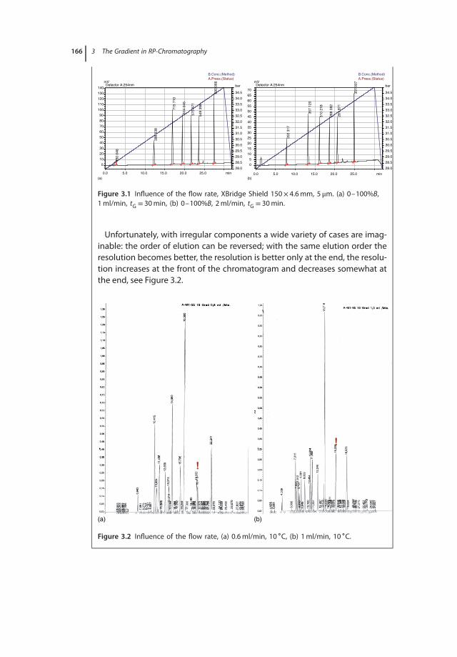
166 3 The Gradient in RP-Chromatography

0.0 5.0

(a) (b)

10.0 15.0 20.0 25.0 min

0

10

20

30

40

50

60

70

80

90

100

110

120

130

140

mV

28.0

28.5

29.0

29.5

30.0

30.5

31.0

31.5

32.0

32.5

33.0

33.5

34.0

34.5

bar

A.Press.(Status)

B.Conc.(Method)

Detector A:254nm

130 0

46

398 5

38

715 7

10

614 0

45

575 8

71

549 3

98

690 0

66

0.0 5.0 10.0 15.0 20.0 25.0 min

0

5

10

15

20

25

30

35

40

45

50

55

60

65

70

mV

28.0

28.5

29.0

29.5

30.0

30.5

31.0

31.5

32.0

32.5

33.0

33.5

34.0

34.5

bar

A.Press.(Status)

B.Conc.(Method)

Detector A:254nm

202 3

17

357 1

20

310 2

18

288 0

82

281 8

71

351 0

07

Figure 3.1 Influence of the flow rate, XBridge Shield 150× 4.6 mm, 5 μm. (a) 0–100%B,1 ml/min, tG = 30 min, (b) 0–100%B, 2 ml/min, tG = 30 min.

Unfortunately, with irregular components a wide variety of cases are imag-inable: the order of elution can be reversed; with the same elution order theresolution becomes better, the resolution is better only at the end, the resolu-tion increases at the front of the chromatogram and decreases somewhat atthe end, see Figure 3.2.

!

!

Seite 3

(b)(a)

Figure 3.2 Influence of the flow rate, (a) 0.6 ml/min, 10 ∘C, (b) 1 ml/min, 10 ∘C.

3.1 Aspects of Gradient Optimization 167

Case 2 The Gradient Duration Is Halved and the Flow Increasedby a Factor of 2

In this case, the gradient volume remains constant, ideally the same chro-matogram (same resolution) is obtained, however, in the half of the time,see Figure 3.3. Often the resolution becomes a little worse, in the case of fastkinetics however the loss of resolution is rather limited.

0.0 5.0

(a) (b)

10.0 15.0 20.0 25.0 min–10

0

10

20

30

40

50

60

70

80

90

100

110

120

130

140

mV

28.0

28.5

29.0

29.5

30.0

30.5

31.0

31.5

32.0

32.5

33.0

33.5

34.0

34.5

bar

A.Press.(Status)B.Conc.(Method)

Detector A:254nm

451 8

29 768 7

64

1 4

25 4

86

1 2

18 4

27

1 1

30 1

93

1 0

55 0

86

1 365050

0.0 2.5 5.0 7.5 10.0 12.5 15.0 min

0

10

20

30

40

50

60

70

80

90

100

110

120

mV

28.0

28.5

29.0

29.5

30.0

30.5

31.0

31.5

32.0

32.5

33.0

33.5

34.0

34.5

bar

A.Press.(Status)B.Conc.(Method)

Detector A:254nm

233 9

79

381 0

93

692 8

04

608 6

10

563 9

15

527 5

12

679 6

77

Figure 3.3 Influence of the flow rate, XBridge Shield, 150× 4.6 mm, 5 μm, (a) 50–90%B,0.5 ml/min, tG = 30 min, (b) 50–90%B, 1 ml/min, tG = 15 min.

The gradient duration is not as important as generally assumed. For6–8 peaks a gradient longer than about 5–7 min is rarely necessary, seeFigure 3.4.

0

0

1 Det.A Ch1/254nm min

0.8

76

1.9

83

2.6

72

3.1

98

3.7

48

4.2

56

5.4

06

50

100

Det.A Ch1mV

1 2 3 4 5 6 7 8

Figure 3.4 The gradient duration required, Zorbax SB C8, 150× 4.6 mm, 5 μm, 40–90%B,tG = 5 min, 2 ml/min.

168 3 The Gradient in RP-Chromatography

0.0 5.0

(a) (b)

10.0 15.0 20.0 25.0 min

0

25

50

75

100

125

150

175

200

225

mV

28.0

28.5

29.0

29.5

30.0

30.5

31.0

31.5

32.0

32.5

33.0

33.5

34.0

34.5

bar

A.Press.(Status)

B.Conc.(Method)

Detector A:254nm 427 9

53

779 9

58

1 4

25 3

47

1 2

20 2

62

1 1

51 2

19

1 0

68 8

88

113 2

29

1 3

93 5

65

0.0 5.0 10.0 15.0 20.0 25.0 min

0102030405060708090

100110120130140150160170180

mV

28.0

28.5

29.0

29.5

30.0

30.5

31.0

31.5

32.0

32.5

33.0

33.5

34.0

34.5

bar

A.Press.(Status)

B.Conc.(Method)

Detector A:254nm

460 6

01

769 9

09

1 4

20 8

81

1 2

24 8

12

1 1

67 9

85

1 0

55 8

36

1 3

55 5

25

Figure 3.5 Effect of initial %B, XBridge Shield, 150× 4.6 mm, 5 μm, (a) 0–100%B, 0.5 ml/min,tG = 30 min, (b) 40–100%B, 0.5 ml/min, tG = 30 min.

Initial and Final %B, Slope As already mentioned earlier, the common practicein method development for an unknown sample, to start with a gradient of, forexample, 5–100%B, rarely proves to be wise: often the first peaks of interest startto elute relatively late. Another disadvantage is that impurities from the waterappear as small interfering peaks (“ghost peaks”). A start at about 40%B oftenhas the following advantages: the peaks are distributed evenly over the wholechromatogram, small interfering peaks seldom emerge, the peaks elute earlier,are narrower and higher, see Figure 3.5. In our view, a start with 0–5%B onlymakes sense if strongly polar components are to be separated on a C18 column,when peaks directly at the dead time are expected. The situation is similar withan isocratic step at the start: only in the case of early peaks and a gradient startwith a high aqueous portion is an improvement in the separation to be expected.

If the number of peaks is known, with the aim of improving the detection limitone can easily start with an even higher %B, see Figure 3.6.

Note:The initial %B is relatively unimportant for the elution of the last peaks, the same

with an isocratic step at the beginning. To put it simply, what happens at the “front”hardly concerns the later peaks. Conversely, the final %B hardly affects what hap-pens in the first third of the chromatogram, this means: initial %B is important forthe “front,” final %B for the “end.” Further, a steep gradient lowers the detectionlimit, a flat gradient often leads to an improvement in resolution only in the laterpart of the chromatogram. Consider Figure 3.7, where the following two gradientsare shown, 40–100%B and 50–90%B. With almost the same gradient duration is,with 50–90%B, the peak height in the first half of the chromatogram large, theresolution small, with 40–100%B exactly the opposite. Depending on the choiceof initial %B and slope, one can selectively influence both resolution and detectionlimit in the front and rear areas of the chromatogram.

Note that in the case of irregular components, an extension of the gradientduration and/or modification of the initial or end %B – and thus the slope – canlead to a reversal of the order of elution, to co-elution, to an improvement of the

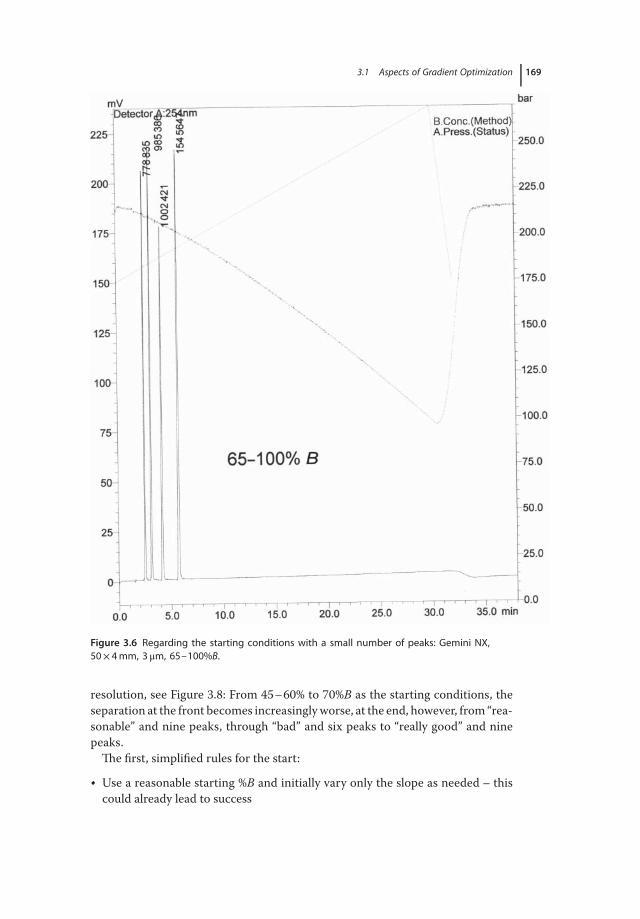
3.1 Aspects of Gradient Optimization 169

Figure 3.6 Regarding the starting conditions with a small number of peaks: Gemini NX,50× 4 mm, 3 μm, 65–100%B.

resolution, see Figure 3.8: From 45–60% to 70%B as the starting conditions, theseparation at the front becomes increasingly worse, at the end, however, from “rea-sonable” and nine peaks, through “bad” and six peaks to “really good” and ninepeaks.

The first, simplified rules for the start:

• Use a reasonable starting %B and initially vary only the slope as needed – thiscould already lead to success

170 3 The Gradient in RP-Chromatography

0.0 2.5 5.0 7.5 10.0 12.5 min

05

101520253035404550556065707580

mV

28.0

28.5

29.0

29.5

30.0

30.5

31.0

31.5

32.0

32.5

33.0

33.5

34.0

34.5

bar

A.Press.(Status)B.Conc.(Method)Detector A:254nm

117 6

67

201 7

27

359 9

95

318 3

80

296 4

48

277 1

73

358 7

33

2.5

(a) (b)

5.0 7.5 10.0 12.5 min

0

5

10

15

20

25

30

35

40

45

50

55

60

65

70

75mV

28.0

28.5

29.0

29.5

30.0

30.5

31.0

31.5

32.0

32.5

33.0

33.5

34.0

34.5

bar

A.Press.(Status)B.Conc.(Method)Detector A:254nm

122 5

10

203 4

02 3

62 5

02

320 0

40

297 6

72

278 6

83

356 9

96

Figure 3.7 Effect of initial %B and slope, XBridge Shield, 150× 4.6 mm, 5 μm, (a) 40–100%B,2 ml/min, tG = 15 min, (b) 50–90%B, 2 ml/min, tG = 15 min.

(a)

(b)

Figure 3.8 Influence of initial %B and slope, Symmetry C18 150× 4.6, 5 μm initial %B: (c)45%, (b) 60%, (c) 70%; final %B in all cases 100%.

3.1 Aspects of Gradient Optimization 171

(c)

Figure 3.8 (Continued)

• Constant slope and modification ofΔ%B – that means parallel gradient profiles,similar chromatograms

• Constant Δ%B and modification of the slope – that probably leads to differentchromatograms

Initial and final %B and gradient duration – they determine the slope – orrespectively column length and flow

As mentioned earlier, the two most important parameters for the resolution are%B/min (strictly speaking %B/ml) and the gradient volume.

Consider the two following cases:

1) In three gradient runs, from 10% to 100%B in 30 min, from 10% to 50%B in13 min and from 10% to 40%B in 10 min, %B/min remains more or less con-stant (about Δ 3%B/min), the result is the same resolution but with differentgradient durations.

2) In three gradient runs, all from 10% to 90%B in 20 min, the last peak elutesat 0.5 ml/min in 16 min, at 1 ml/min in 8 min and at 2 ml/min in 4 min. Heretoo, %B/min remains constant, the result is the same resolution (the gradientvolume remains constant at 8 ml), the retention time of the last peak howeverbecomes increasingly lower.

Following a change in the slope due to a change in the initial %B and/or thegradient duration, with irregular analytes one should expect both a change in theelution order as well as an improvement or deterioration of the resolution, seeFigure 3.9. Note the following: the gradient becomes flatter and longer, which givesa slope of Δ 16%B/min through Δ 7%B/min to Δ 3.3%B/min. What do you notice?In spite of this large difference, the separation of the first four peaks is only slightly

172 3 The Gradient in RP-Chromatography

affected. The chromatogram varies significantly only after the fourth peak, withchanges in the order of elution and in the resolution (8 vs. 10 peaks).

Once again: in the case of not very difficult separations gradient duration andcolumn length are not so important, see Figures 3.10 and 3.11. When one knowsthat only these seven peaks are to be expected, a 20 mm× 4.6 mm, 2 μm column issufficient, a 150 mm× 4.6 mm, 4 μm column inevitably brings unnecessarily long

(a)

(b)

Figure 3.9 Effect of initial %B and gradient duration on elution order and resolution, Ascen-tisExpress C18, 50× 3 mm, 2.7 μm, (c) 20–70%B, tG = 15 min, (b) 20–90%B, tG = 10 min, (a)10–90%B, tG = 5 min.

3.1 Aspects of Gradient Optimization 173

(c)

Figure 3.9 (Continued)

retention times. Figure 3.11 (column: 20 mm× 4 mm, 2 μm), demonstrates whathas already been described earlier. First, in spite of a small column volume andalso a considerable dead volume of the apparatus the peaks look useful, the peakwidth remains constant. Secondly, for this small number of peaks a 2 cm column issufficient. And thirdly, a 2 min gradient compared with a 10 min gradient is equallysufficient (the drift in the lower image and the apparently broader peaks are noproblem, the scaling is different).

Of course, with ≤2 μm particles and/or 20 mm columns, fused core materials,high throughput columns and Chromolith HR, we have noticed tailing andpeak broadening due to the instrumental dead volume, especially with the earlypeaks – even with modern equipment! But for simple separations we can livewith the loss of 20–40% efficiency, because whether a peak has a peak widthof 3 or 4 s will, due to the narrow peak form and a satisfactory separation,not usually be registered from the user as a disadvantage – and then it is noproblem.

Now to conclude, some aphorisms regarding gradients as a compressed “take-home message,” many a repetition of the previous text is acceptable here.

3.1.7Gradient Aphorisms

Flow• The resolution of later eluting peaks is more likely to be strongly negatively influ-

enced by an increase in flow than that of earlier eluting peaks• Increase in flow may change the selectivity/resolution• Use a high flow with small particles and “simple” interactions

174 3 The Gradient in RP-Chromatography

40

30

20

10

10

5

0

0 1 2 3 4 5 6

0

0.0 2.5(a)

(b)

0.9

32

0.2

22

0.6

54

1.0

51

1.7

03

2.5

71

3.4

72

5.9

00

2.9

23

4.4

38

6.8

52

10

.12

5

13

.613

22

.36

2

5.0 7.5 10.0 12.5 15.0

Det.A Ch1

Detector A

H:\Kuss\Gradiententest93.lcd

F:\lexar\Stavros\Gradiententest100.lcd

17.5 20.0 22.5min

min

Figure 3.10 Influence of column length, (b) Synergi Fusion RP, 150× 4.6 mm, 4 μm, (a) Syn-ergi Fusion RP, 20× 4.6 mm, 2 μm.

• Use a low flow with≥5 μm particles, but also in the case of multiple interactions,that is, when slow kinetics are expected

• Try a high flow first when Δ%B is ≥60%

Gradient duration

• The gradient duration is not as important as is generally believed, as a rule ofthumb: gradient duration about 10–15 times the dead time

• If you use a long gradient, at least increase the flow

The initial and final %B, Δ%B

• In general, Δ%B and gradient volume are the most important factorswith respect to optimization, in practice – not always appropriately – the

3.1 Aspects of Gradient Optimization 175

gradient duration is often changed instead of the flow. Consequently, essentialoptimization parameters are Δ%B and gradient duration and from these theslope

• With differing components, a Δ%B≥ 40 is necessary• The elution strength is more important than the flow, with the same gradient

duration and twice the flow, the peaks elute only about 10% earlier• Start with, for example, 30–40%B, increase to 100%B and wait a few minutes

to make sure that all the peaks elute during the gradient and not in the flushingphase. Then make the gradient flatter to test whether the resolution improves.Note as a general rule, the initial %B should so be chosen that the first peaks ofinterest elute after approximately two to three times the dead time – don’t startunnecessarily with a high aqueous percentage. Choose the final %B so that all

H:\Kuss\Gradiententest89.lcd

Det.A Ch1

Det.A Ch1

H:\Kuss\Gradiententest88.lcd

40

30

30

40

50

20

10

0

0.0 0.5 1.0 1.5 2.0 2.5 3.0 3.5 4.0 4.5 5.0

20

10

0

0(a)

(b)

1 2 3 4 5 6

0.1

06

0.3

70

0.5

57

1.016

1.781

2.7

20

5.2

01

min

min

0.1

09

1.427

1.949

3.1

68

0.9

24

0.5

53

0.3

75

Figure 3.11 Influence of gradient duration, Synergi MAX RP 20× 4 mm, 2 μm, (a) gradientduration 2 min, (b) 5 min, (c) 10 min.

176 3 The Gradient in RP-Chromatography

20

10

0

0.00 0.25 0.50 0.75 1.00 1.50 1.75 2.00min

1.25(c)

Det.A Ch1

H:\Kuss\Gradiententest87.lcd

0.1

12

0.3

84

0.5

29

0.7

63

1.0

07

1.2

23

1.6

73

Figure 3.11 (Continued)

peaks which are to be separated actually elute – in no case choose a higher end%B, otherwise the gradient takes unnecessarily long and during this time noth-ing more happens. After elution of the last component, one should of courseincrease (fast, steep) the organic content to 100%B to flush the column. Theflushing time depends on the matrix, the other organic impurities and the addi-tives in the eluent, and is usually 5–10 column volumes.

Length of the column

20–30 mm, for about 5–8 peaks50 mm, for about 8–12 peaks100–125 mm, for about 20–25 peaks

Assumption: no additional peaks, for example, from a difficult matrix

• Gradient volume (and Δ%B): much more important than the column volume• Short column (and small particles)? Short gradient• Long column? Longer gradient plus higher flow• Short gradient? Length of the column rather unimportant

Gradient slope and …• The steeper the gradient, the less the influence of the length of the column

on the resolution• The steeper the gradient, the less important the flow becomes• Initial %B is more important for the first half of the gradient than the gra-

dient slope• The higher %B is at the start, the less of an advantage is, for example, a

30 min over a 20 min long gradient

3.2 Prediction of Gradients 177

In general• High peak capacity does not automatically mean good resolution overall• The gradient compensates dead volume in the instrument and poor pack-

ing quality, a high plate number makes itself significantly noticeable onlywith really difficult separations

• The linear gradient model is sometimes insufficient, for example, oftenfrom about 80%B – here especially with acetonitrile – and in the case ofadditional ionic interactions, see Section 3.2.

Be courageous, when you have about ≤10 peaks and a relatively clean sample,then proceed as follows: short column, high flow, short, steep gradient starting atabout 30–40%B.

Be consequent, when you expect about ≥30–40 peaks and have a UHPLC, thenuse a 150× 3 or 2,1 mm, 2 μm column, run a steep gradient and make sure thatyou have a gradient volume of about 25–30 ml. Subsequently run two gradientsat two temperatures differing by about 30 ∘C, a long one with a low flow and a shortone at a high flow – and keep an eye on the gradient volume. For 30–40 peaks, agradient volume larger than 30 ml for this column volume is not usually necessary.However, do you expect this number of peaks in a really difficult matrix, and overand above that are you aiming for a robust method? In this case, think of 3.5 oreven 5 μm particles, maybe also of a 4 mm or even 4.6 mm column.

3.2Prediction of GradientsHans-Joachim Kuss

3.2.1Linear Model: Prediction from Two Chromatograms

With only two chromatograms at appropriate isocratic conditions, the retentiontimes for all other isocratic conditions can be predicted provisionally. Assumethat we have a 15 cm SunFire column in the drawer as well as a test mixture ofmethyl-, ethyl-, propyl-, and butyl-paraben. Then we can start with, for example,55% methanol and 45% water and obtain the chromatogram in Figure 3.12.

We can use our gradient system to make this eluent mixture. The horizontalline in all chromatograms shown in this chapter represents the set value of themethanol content, the rather uneven line the measured pressure. Both parametersshould always be displayed as error indicators.

Now we have made an isocratic overview run and can see the four peaks withincreasing retention times tR in the above-mentioned order. Knowing the mobiletime (formerly called dead time) of t0 = 0.75 min (small peak, calculation seebelow) we can also calculate the retention factor k, which generally should be not

178 3 The Gradient in RP-Chromatography

Figure 3.12 Parabens on a 150× 4.6 mm SunFire 2 ml/min 55% MeOH/45% water at roomtemperature. The peak widths w50% are 0.078; 0.115; 0.191; 0.365.

Figure 3.13 Parabens on a 150× 4.6 mm SunFire 2 ml/min 70% MeOH/30% water at roomtemperature. The peak widths w50% are 0.052; 0.058; 0.074; 0.098.

lower than 0.5. Methyl paraben has a k of 2.1. Therefore, a second measurementcan be carried out at a higher methanol concentration, for example, at 70%B, asin Figure 3.13.

3.2.1.1 What Does the Retention Factor k Tell Us?The retention time tR is the primary variable in chromatography, from which wededuce whether an analyte is present or not. The retention times tR are dependenton the column dimensions. When under the same conditions a column with threetimes the length L is used, then the retention times and t0 increase by a factor of 3.A column with half the internal diameter dc, that is, a quarter of the cross-section,reduces at the same flow rate the retention times and t0 by a factor of 4.

To convert the retention times into the dimensionless retention factors k themobile time t0 is needed, which is calculated from the mobile volume V 0 and theflow F [7]. The mobile volume can be estimated from the internal volume of thecolumn and a characteristic factor for the packing.

V0 ≈ 0, 5d2c L (3.6a)

t0 =V0F

(3.6b)

3.2 Prediction of Gradients 179

When L and dc are in centimeter, then V 0 is in milliliter. No separation can occurduring t0, and so in the first step t0 is subtracted from tR. This gives the additionalhold-up time in the stationary phase ts. The relativization of tS through the mobiletime t0 eliminates the influence of varying column dimensions.

k =tR − t0

t0=

tst0

(3.7)

The retention factor k depends on the interaction of the analytes with the respec-tive column material but not on the column diameter dc, the flow F , the columnlength L or the particle diameter dp.

The retention factor k is a measure of the interactionAccording to the Linear Solvent Strength Model [8], in RP HPLC k is logarith-

mically dependant on the percentage of the organic fraction %B, this means that agraph of ln(k) against %B results in a straight line for each substance under analysiswith a large k00 for pure water and a characteristic ln(k)-slope S.

ln(k) = ln(k00) − S%B (3.8)

The slope S is an individual, characteristic variable and dependant on thesubstance and the current interactions with the phase material. In the above-mentioned example (compare Figure 3.14), the four k-values are calculated andfrom them the ln(k) values. With the Excel functions “slope” and “intercept” thetwo characteristic straight line parameters are found. Then, for any other %Bconditions the ln(k) and from them the k-values can be calculated and converted

Figure 3.14 Detail from “2SIS SunFire MeOH.xls.” The dark grey shaded cells contain theinput data. The bar in row 28 is a scroll bar that changes the value of %B in cell B13 andshows dynamically the chromatogram.

180 3 The Gradient in RP-Chromatography

into retention times. With increasing chain length the parabens have much largerk00-values, but also larger S values.

The usable gradient range 𝛥%B=%Be −%Ba (final value minus initial value)depends only on the conditions for the first and the last peak. We look for theleftmost and rightmost intersections of the straight line with the horizontal linefor ln(k)= 0, that is, k = 1. The %B value of the left intersection is the maximuminitial value of the organic modifier %Ba,max for both isocratic and gradientseparations. Higher %B values as %Ba,max lead to k-values less than 1, whichshould be avoided. Initial conditions of %Ba greater than %Ba,max lead to the firstpeak being eluted too early and possibly unsatisfactorily separated. But lowerinitial conditions as %Ba can be set and thereby the separation modified. Thisvariable is, therefore, in addition to tg an optimization parameter. In Figure 3.3,the %Ba,max in the ln(k) graph is shown as 66% MeOH. All four intersections canbe calculated by dividing the intercept by the slope (see Figure 3.14, cells C2 toF2). In the cell I1, the minimum value of the intersections is requested and shownas 66%.

The right-hand intersection is a first guess of the %B-conditions by which thelast peak must be eluted. Higher end values of %Be do not alter the separation asthe substances have already been eluted and no longer “see” the continued run-ning of the gradient. Therefore, in the calculations %Be is set to 100%. For the realmeasurement of chromatograms %Be is reduced so far at constant gradient slopeΔ%B/tg that the last peak remains “in the gradient.”

When the difference %Be – %Ba between the right and left intersections is largerthan 40% [9], then to obtain all peaks within an acceptable analysis time a gradi-ent must be used. In the above-mentioned example with %Be – %Ba = 15% (see cellK1) no gradient is necessary. The shortest isocratic separation can be made with66% MeOH. When a line is drawn vertically upwards at 66% MeOH, the chro-matogram can almost be “seen” – the distance between the peaks increases, thisis not very apparent on a logarithmic scale. At all %B-conditions visible here thelines are far apart, that is, the peaks have so much space between each other thatthey are very well separated, as shown by the chromatogram in Figure 3.14.

From a ln(k) versus %B graph the retention factors can be calculated for each(not measured) mixing ratio %B and thus for a given column dimension the reten-tion times. With the retention times, the corresponding isocratic chromatogramcan be visualized. The simulation of chromatograms from the report data is donewith the Excel function “Normdist” [10].

The file “2SIS SunFire MeOH.xls” shows through movement of the scroll barthat with %B= 0%, that is, pure water, an analysis time of 3 days would be requiredand that between 90% and 100% the peaks coincide near t0. SIS stands for Sin-gle Isocratic Steps. In principle, the ln(k) versus %B-graph contains all the datarequired for the prediction of gradients, for this the integral over many isocraticconditions must be made. The “programming” of gradient prediction in Excelaccording to the linear model has been described in detail by Neue [11].

3.2 Prediction of Gradients 181

3.2.1.2 What Do the Two Retention Factors kg and ke Mean?Imagine a car which, after a certain distance, passes through a light barrier atconstant speed. Depending on the speed both the (retention) time tR and the dura-tion of the passage through the light barrier (= peak width w) are equally shorteror longer, so that tR/w is constant. Remember that in chromatography tR

2/wb2 is

proportional to the plate number N . The peak width wb can be determined asymp-totically.

Then imagine a car moving at different speeds. The retention time depends onthe integral of the speed, that is, from all speeds on the route. For the peak widthonly the speed when passing through the light barrier is relevant, no matter whathas happened before.

In a gradient, both kg (dependant on the course of the gradient) and ke (depen-dant only on %B at the moment of exit from the column) must be calculated [11].So on the face of it the retention factor kg corresponds to the integral (simplified:the “average”) of the individual retention factors over the entire gradient under theselected conditions, while ke is the retention factor at the moment of elution/exitfrom the column. As with the above-mentioned analogy, the retention time is cal-culated from kg and the peak width from ke. In isocratic separations, kg and kecoincide. The gradient slope G is explained below (Section 3.2).

kg =1

GSln(k0GS + 1) (3.9a)

ke =k0

GS k0 + 1(3.9b)

kg > ke (3.9c)

The driving force in chromatography is the elution strength %B. In the chro-matogram, in Figure 3.15 %B was changed from 55% to 70% methanol after 5 min.The first two peaks were eluted with only 55%, the last two peaks at first with55% and then with 70%. The third and fourth peaks have a considerably longer

Figure 3.15 Parabens on a 150× 4.6 mm SunFire 2 ml/min 55% MeOH for 5 min, then 70%MeOH at room temperature. The peak widths w50% are 0.079; 0.116; 0.071; 0.093.

182 3 The Gradient in RP-Chromatography

Instrument Parameters View

Data Acquisition

Filename:

100

75

50

25

00.0 2.5 5.0 7.5 10.0 12.5 15.0 17.5 20.0 22.5 25.0

RT:0.000 min Ch#:

Max Intensity : 0

75.0

50.0

25.0

0.0

%

LC Time Prog. Pump Detector A Controller Autosampler Auto Purge

Normal Advanced

Figure 3.16 Gradient from 5% to 100%B in 20 min in the method file from Labsolutions(Shimadzu).

retention time than isocratically with 70%, but the peak width is identical to the70% run.

3.2.1.3 How Does the Integration- and Control System See the Gradient?With a simple linear gradient, the initial and end times of the gradient togetherwith the two %B-values are entered into a table. The Gradient time tg is calculatedfrom the difference of the two times (Figure 3.16).

The instrumental gradient slope is obtained from the quotient:

Δ%Btg

The profile is presented graphically, including the return to the initial conditionsafter the gradient. After again reaching 5%B, 5–10 times t0 have to be waited forequilibration of the column. When the column dimension (t0) is not defined, thentg cannot be rated as short or long.

When, for example, only the region of 20–80% MeOH is used, then to improvemixing it is useful to pre-mix the initial and final %B. The %B set instrumentallyis then no longer identical with the real methanol content (also called Φ), but canbe used directly just the same.

3.2.1.4 How Does the HPLC-Column See the Gradient?As with the k-values, the relativization to the column dimensions is made bymeans of the relation of tg to t0. This gives the effective gradient slope G. Thequotient tg/t0 is a measure of how many times the mobile volume of the columnflows through it during the gradient.

G =t0Δ%B

tg=

Δ%BV0tgF

(3.10)

During a gradient, the analytes are moved by two driving forces. On the one handat constant speed, dependant on the flow, on the other hand with increasing speed,

3.2 Prediction of Gradients 183

due to the gradient slope. Both effects complement each other multiplicatively.When I double the flow, then I have to halve the gradient slope if I want to getthe same gradient and chromatogram, resulting in the same separation in half theanalysis time.

Two columns 25 cm 5𝜇 and 15 cm 3𝜇 with the same RP-material also give thesame separation when tg/t0 =V g/V 0 remains constant. This means that at thesame flow, tg and parallel to this t0 of the shorter column must be 5/3 lower inorder to obtain exactly the same k-values for all analytes. The analysis time isreduced accordingly. Because the expected number of plates in both columns isabout 10 000, the peak widths relative to the retention times are the same.

We have three instrumental variables: %Ba, F , and tg/t0. I can reduce the maxi-mum initial concentration %Ba from the maximum value %Ba,max down to 0% (onlywith water compatible columns, otherwise 5% or 10%), usually I can increase theflow only by a factor of 2 or 3, so that tg/t0 remains as the main variable, which Ican alter in the region of about 3–60.

3.2.1.5 How Do the Substances to Be Analyzed See the Gradient?The individual analytes “experience” the gradient differently. The initial %Ba is thesame, but each substance “sees” the gradient only until it leaves the column in theeluent with the %B current at this time. The effective gradient slope G is equal forall substances, but is modified by the varying influence of the organic modifier %Bon the interactions, which is measured by the ln(k)-Slope S.

GS =Δ%Bt0S

tg(3.11)

This is the intrinsic gradient slope (GS) individually effective on the analytes. Theinstrumental gradient slope G acts on a column of defined dimensions, and inconjunction with the interaction of each analyte with the column material usedthe substances are eluted. I have to work with the intrinsic GS, but I am free tochange the eluent or to use a column with preferably other characteristics in orderto change the interaction and thus the retention.

3.2.1.6 Interpretation of the ln(k) to %B GraphThis graph is the focal point for the gradient. From it can be estimated how difficultit will be to optimize a separation. The more substances that have to be analyzed,the more difficult the assignment of the peaks will be.

When in Figure 3.17 at a methanol content of, for example, 40% you move slowlyvertically upwards, you pass through the isocratic chromatogram again. The dis-tance between the straight lines corresponds to the distance between the peaks.The critical peak pair chlorobenzene/toluene can immediately be seen. With agradient you go from %Ba diagonally up toward the right to %Be. However thegradient is also, and strongly, dependent on the gradient duration tg.

The intersections indicate conditions %B where two peaks directly coincide andwhere a change in the peak order occurs, that is, a point to be avoided. If thereare many intersections, which of course becomes more likely with an increasing

184 3 The Gradient in RP-Chromatography

1

2

3

4

35% 45% 55% 65% 75%

%B

ln(k

)

Figure 3.17 ln(k) versus %B graph on a150× 4.6 SunFire 5𝜇 at 30 ∘C. The fourdashed lines are the four parabens inFigures 3.1–3.153.4. The solid lines from

bottom to top are phenol, benzaldehyde andbenzene, followed by the two closely adja-cent straight lines corresponding to tolueneand chlorobenzene.

number of analytes, then the separation problem is difficult. When the intersec-tions are widely distributed relative to %B, the separation problem becomes evenmore difficult as several %B must then be avoided.

The probability of obtaining intersections is large with chemically different ana-lytes, as the interactions with the stationary phase will differ. The more substancesto be separated, then the sooner intersections become inevitable. Especially com-plicated are adjacent lines, that is, analytes with similar retention times and similarslopes. When the lines directly overlap then the separation problem cannot besolved, even with a gradient.

The separation factor 𝜶 is the distance between the straight linesThe separation factor 𝛼 is the quotient of the k-values of two neighboring peaks.

The larger value (following peak) is always divided by the smaller value (precedingpeak). A chromatogram with several peaks, all having 𝛼 = 1.05, means that forall peak pairs the second peak has a k-value about 5% higher than the respectivefirst peak

𝛼 =k2k1

=tR2 − tmtR1 − tm

=tS2tS1

(3.12)

The separation factor 𝛼 (formerly: selectivity factor) is the quotient of the twohold-up times in the stationary phase, that is, the relative interaction strength ofa peak pair. Instead of 𝛼 the value 𝛼 − 1 in percent can be used, that is, instead of𝛼 = 1.05 then 𝛼 − 1= 5%, which is much easier to visualize.

3.2 Prediction of Gradients 185

With a glance at Figure 3.17 it can be seen that the separation problem hasbecome difficult due to the five substances present in addition to the parabens.Phenol and benzaldehyde (bottom left) separate well over the entire %B range.In Figure 3.6, four intersections can be seen and a further intersection for ethylparaben and benzene at about 30% can be suspected.

A ln(k)-axis is basically also a linear 𝛼-axis, because an equal interval in thelogarithm of two values means the same quotient: 𝛼 = k2/k1. The logarithm of 1.05(the 𝛼 value necessary for a resolution greater than 1 with 10 000 theoretical plates)is 0.05. This means that when the ln(k) axis has a 0.05 grid, then the conditionwhere ln(𝛼)> 0.05 is reached can easily be seen. The interval of the lines must beat least one vertical box.

If the polarity of the analytes differs so much that they can be separated iso-cratically only in an unacceptably long analysis time, then a gradient is essential.If for each peak pair no differing isocratic conditions in which adequate separa-tion results exist, then a gradient cannot be successful either. This can be seen byexactly overlying lines in the ln(k) versus %B-graph. This is a rare but possible case.

The main problem immediately recognizable, the separation of the nine sub-stances on a SunFire column, is due to the very similar manner of interaction oftoluene and chlorobenzene, which coincide by 55% methanol. Only at %B= 35%or at B= 75% are the lines separated by ln(k)= 0.05 (one box vertically). At 75% thefront peaks have almost no retention. Therefore, in the isocratic mode this sepa-ration problem can only be solved with a methanol content of 35% or lower. Then,however, the last peak butyl paraben has a ln(k)-value of 4.75, that is, k = 115.6,and a retention time of 175 min. So here there is no acceptable isocratic chro-matogram.

With the calculation of kg all chromatograms with a simple linear gradient canbe predicted. As an initial value %Ba,max is chosen as the first step and %Be set to100%. In contrast to real chromatography, no time is lost when the gradient runsfurther unnecessarily. Then tg/t0 is varied in the range of 3–60 in increments ofone, and all values for kg are calculated. Excel then calculates the retention times,which can be sorted by the function Small (); see Figure 3.18.

3.2.1.7 The Instrumental Gradient Delay (Dwell Time)The gradient at the column outlet lags behind the start of the gradient throughthe system controller by the gradient delay time (Dwell Time) td. During thistime, the analytes move with the initial gradient conditions %Ba isocratically.The instrument-specific time td must be taken into account when transferringgradient separations from one instrument to another. Regarding this problem inthe UHPLC and with LC/MS-gradient separations, see Section 1.2.

The dwell time is best measured under realistic conditions, for example, with%B= 0–100% in 15 min. Instead of the column a capillary with preferably smallinternal diameter is used, in order to build up a realistic back pressure whileincreasing the volume as little as possible. Eluent A is water, eluent B water with afew parts per thousand of acetone. When the UV absorbance is set to zero, eluentB should have a maximum absorption of slightly less than 1 AU. The gradient is

186 3 The Gradient in RP-Chromatography

0.7

0.6

0.5

0.4

0.3

0.2

0.1

00

Phenol

2.51

%Be-%B

a

4.5 tg + t

0 = 6.0076

N = 100001.5076

89%

t0 =35%

54%

k00 31.6253421

6.657290689

0.868508238

0.780633664

0.663044327

0.517589444

32.23372059

5.775980339

1.424732027

0.677291244

0.99731267

0.72506977

152.2351591

8.023965133

1.998676582

0.940889859

1.124441789

0.693856145

366.6079135

8.460887974

3.801567248

0.992123416

1.575093037

0.796703039

1153.803715

9.250199291

7.812396166

1.084678032

2.073006205

0.824620032

4258.777006

10.30675601

16.29876058

1.208569834

2.507133795

0.787448578

206.7328402

6.553014303

6.006244083

0.768406219

2.245535567

1.069633552

778.4529407

7.650125777

12.50640135

0.89705347

2.790229228

1.023528335

955.7138911

8.025863056

12.5345965

0.94111241

2.708676329

0.979535924

Bk

0

Gk

g

ke

%Ba

%Be =

3.01 3.20 3.88 4.63 5.29 4.89 5.59 5.71

Benzaldehyde Methylparabene Ethylparabene Propylparabene Butylparabene Benzene Chlorbenzene Toluene

tR

tG

1 2 3 4 5 6 7−0.1

Phenol

Benzaldehyde

Methylparabene

Ethyparabene

Propylparabene

Butylparabene

Benzene

Chlorbenzene

Toluene

Figure 3.18 Shows the calculation and the predicted chromatogram with a satisfactory sep-aration using the linear data of Figure 3.17 (listed in the lower part of Table 3.2).

c

tg

1 2 43 5 6

20%

40%

60%

80%

100% tD t0

Figure 3.19 At the end of the column, the analytes exit delayed by the dwell time td andthe mobile time t0.

run and the time t50% determined, which is when half the maximum absorption isreached. To obtain the dwell time, half the gradient time is subtracted from t50%(Figure 3.19).

The dwell time td is a (hopefully) short isocratic separation preceding the gradi-ent. Therefore, td must be taken into account in the equations. Before the eluentreaches the column outlet, additionally t0 elapses (see Figure 3.17). Only whenthe analyte has left the column can it no longer be affected by the continued run-ning of the gradient. In Figure 3.15, the third peak, which comes about 1.3 minafter the eluent change, is clearly eluted in 70% MeOH. Also the base line offsetand the pressure profile indicate that td + t0 is about 1 min. At a flow of 2 ml/min

3.2 Prediction of Gradients 187

t0 ≈ 0.75 min and td ≈ 0.25 min, and so the dwell volume can be estimated at about0.5 ml. A more accurate measurement as described here results in a dwell volumeof 0.325 ml.

During td, the analytes move with different speeds and with an individual reten-tion factor k at the initial conditions %Ba through the column:

tdtR

=td

t0(k0 + 1)(3.13)

Substances with long retention times are relatively unaffected, on the other handsubstances with short retention times and small retention factors k0 are stronglyaffected.

The mobile time is the sum of an isocratic fraction t0,d and a gradient fractiont0,g. (Note: The mobile or dead time remains of course overall unchanged, becausewhether 100% water or 100% acetonitrile is used is irrelevant for the elution of antrue inert component, which is influenced only by the column dimensions and theflow. In reality, there is a slight influence:

t0 = t0,d + t0,g (3.14a)

andtdtR

=t0,d

t0(3.14b)

Summarized and solved for t0,g, the result is

t0,g = t0 −td

k0 + 1(3.15)

With decreasing k0 the substances have moved further into the column. There-fore, t0,g is different for each substance and only the remaining part of the columnis available for the gradient. Of course, the predetermined instrumental gradientslope does not change, but the effective gradient slope does, as the column avail-able for the gradient has become “shorter.”

The various molecules all move into the column during the same time td. But asthey are retained to varying extents under the initial gradient conditions %Ba theymove different distances, the “early” substances a long way, the “late” substancesnot so far.

The retention factor k0 is different for each substance and for each (initial) elu-ent mix %Ba. This means that during td each substance moves a different distanceinto the column, and this is dependent on %Ba. The “remaining column” availablefor the gradient is, therefore, different every time, which manifests itself in differ-ing t0,g. Of course, the shorter the column used then the shorter the “remainingcolumn” is (see Eq. (3.12): td is constant, but t0 is shorter).

Many HPLC manufacturers now offer the possibility of delayed injection, inwhich the injection is delayed by td after the start of the gradient. With a softwaremodification this should also be possible with older systems. It is not so much amatter of the additional computing effort, rather the noncomparability of gradi-ents on different systems with differing td (Table 3.1).

188 3 The Gradient in RP-Chromatography

Tab

le3.

1C

onta

ins

inth

eup

per

par

tthe

rete

ntio

ntim

esof

the

eigh

tgra

dien

tchr

omat

ogra

ms

with

anin

stru

men

talg

radi

ents

lop

eof

5%M

eOH

/min

.

Rete

nti

onti

mes

usin

ga

100* 3

Ch

rom

olit

h-c

olum

n(t

0=

0,42

75m

in,1

ml/

min

)gra

die

nte

xten

sion

atco

nst

antg

rad

ien

tslo

pe

(5%

B/m

in)

%B

tGPh

enol

Ben

zald

ehyd

eM

ethy

lpar

aben

eB

enze

ne

Ethy

lpar

aben

ePr

opyl

par

aben

eTo

luen

eC

hlo

rob

enze

ne

But

ylp

arab

ene

45–

705

0.96

41.

158

1.39

72.

498

1.99

73.

023.

867

3.86

74.

191

40–

706

1.08

91.

366

1.86

43.

062

2.68

3.86

4.68

44.

684

5.14

735

–70

71.

229

1.53

32.

316

3.69

63.

474

4.76

95.

543

5.54

36.

123

30–

708

1.43

51.

773

2.76

94.

325

4.30

55.

695

6.41

26.

431

7.1

25–

709

1.71

42.

066

3.39

75.

022

5.18

36.

653

7.25

97.

344

8.09

520

–70

102.

075

2.41

34.

134

5.69

56.

112

7.62

88.

168

8.27

49.

093

15–

7011

2.54

52.

822

4.95

66.

371

7.06

98.

614

9.09

29.

217

10.0

9210

–70

123.

138

3.30

55.

844

7.06

28.

041

9.61

310

.03

10.1

7111

.089

Diff

eren

ce6–

50.

125

0.20

80.

467

0.56

40.

683

0.84

0.81

70.

817

0.95

6D

iffer

ence

7–6

0.14

0.16

70.

452

0.63

40.

794

0.90

90.

859

0.85

90.

976

Diff

eren

ce8–

70.

206

0.24

0.45

30.

629

0.83

10.

926

0.86

90.

888

0.97

7D

iffer

ence

9–8

0.27

90.

293

0.62

80.

697

0.87

80.

958

0.84

70.

913

0.99

5D

iffer

ence

10–

90.

361

0.34

70.

737

0.67

30.

929

0.97

50.

909

0.93

0.99

8D

iffer

ence

11–

100.

470.

409

0.82

20.

676

0.95

70.

986

0.92

40.

943

0.99

9D

iffer

ence

12–

110.

593

0.48

30.

888

0.69

10.

972

0.99

90.

938

0.95

40.

997

The

low

erpa

rtof

the

tabl

esh

owst

hese

ven

diffe

renc

esfr

omth

ese

cond

toth

efir

stch

rom

atog

ram

,and

soon

(e.g

.,0.

125m

in=

1.08

9–0.

964)

,tha

tis,

the

addi

tiona

lre

tent

ion

caus

edby

the

exte

nsio

nof

the

grad

ient

.

3.2 Prediction of Gradients 189

3.2.1.8 Extension of the Gradient Downwards by Constant Slope

The earlier gradient start from %Ba = 45% down to 10% in steps of five causes asignificant change in the separation. The two peaks for ethyl paraben and benzeneeven move past each other. Interesting is that the last peak is shifted toward theend only by almost a minute (differences between 0.97 and 1 are shaded gray),this means that butyl paraben in contrast to all earlier peaks remains “stuck”at the front of the column. The peak width of butyl paraben remains constant,although the retention times increase. The elimination concentration does notchange either.

The smaller the differences are, the further the substances move due to therespective “gradient extension.” Only when ln(k)≈ 5, that is, k ≈ 150 do the sub-stances “freeze,” they do not move any further, and without forward movement noseparation is possible. In contrast to propyl paraben, toluene and chlorobenzenedo show a certain degree of mobility despite higher retention times, even in the12-min chromatogram. This is explained by the higher ln(k)-slope of the parabens,through which the ln(k) limit is reached earlier.

It should be noted that by reducing the gradient initial value %Ba more changesare to be expected in the front part of the chromatogram as in the rear section.The upshot of the gradient extension and the dwell time is: when %Ba is reducedfrom its maximum value %B0,max down to zero, then the farther forward that thepeaks come in the chromatogram, the greater is the change in the separation. Thiscan lead to a better separation, but also a change for the worse. In the rear section,only a slightly modified separation is to be expected.

3.2.2Curvilinear Model: More than Two Input Chromatograms

3.2.2.1 The ln(k)-Straight Lines Are Often not Straight at All

When measurements are made at 5–10 different %B values, then the ln(k) valuesoften show a curvature, which is less with methanol and stronger with acetonitrileand tetrahydrofurane. In the equation, the curvature is superimposed over thestraight line and a curvilinear course results. As a result, a two-point linear fit cangive slightly varying intercepts and slopes, depending on which two data pointshave been measured. Furthermore, due to opposite curvature two curves can inreality drift further apart than can be shown with the straight lines. Finally, theopposite curvature can also lead to two intersections, which two straight linescannot have.

Schoenmakers [12] writes in the summary: “Firstly, the relationship between ln kand 𝜙 is generally nonlinear, in accordance with previous statements” and furtherbelow: “Consequently k(𝜙) should correctly be expressed as ln k =A𝜙

2 +B𝜙+C.Snyder and co-workers, conceding this point, nevertheless argue that the linearrelationship provides an adequate approximation for practical gradient elution.”In other words, Schoenmakers proposes describing the curvature with a superim-posed parabola.

190 3 The Gradient in RP-Chromatography

With today’s HPLC instruments running automatically overnight, thenunlike previously it makes little difference whether only 2 instead of 10chromatograms are run. The real effort is in the sample preparation, the pro-gramming of the sample sequence and possibly the preparation of the eluents(Table 3.2).

The data of Table 3.2, whose graphs are shown in Figures 3.17 and 3.20, weretaken during one night. This input mask can be used just as well for only twomeasurements. Chromatograms with a difference of less than 5%B will hardly beneeded. The shaded cells in the first three rows have to be filled in, as they arerepeatedly required further below.

When comparing Figures 3.20 (curved) and 3.17 (linear) with the identicalmeasurement points, it can be seen that the linear fit to all data points sometimesclearly misses these. Not all data points are shown in the figures, in order to showthe section enlarged. In Figure 3.20, two additional intersections can be seenbetween 35% and 40%. The quite significant deviations from reality in Figure 3.17lead even with isocratic predictions to an error of far more than 1%, althoughmethanol causes only slight deviations from linearity. These errors are inevitablycontributory factors in the gradient prediction – if this is based on the linearmodel.

3.2.2.2 The ln(k) to %B Fit According to NeueThe correction of the ln(k) to %B curves can also be described with a hyperbolicfunction [13], which has the advantage that it can be simply integrated. This istaken into account by a curvature factor a. The quadratic function proposed bySchoenmakers [12] sometimes shows a (physically implausible) upturn of ln(k)in the upper %B-region, which however usually lies in the region where the sub-stances have already been eluted.

ln(k) = ln(k00) + 2 ln(1 + a%B) − S%B1 + a%B

(3.16)

The gradient parameters are named differently depending on the author andabbreviated differently. In contrast to [14], %B is used here for the organic fractioninstead of c, the ln(k)-slope named S instead of B and the effective gradient slopeG instead of S.

At the lower end of Table 3.4 the characteristic values %B-slope S and inter-cept ln(k00) for the linear model are calculated directly and the curvature factorset to zero. The three values for the curvilinear model according to Eq. (3.16) aredetermined iteratively using the Excel Solver and copied into the table.

The equations for kg and ke are frighteningly long [14]. Repetitive calculationsare summarized in this chapter in the three auxiliary variables H , I, and J , whichare built successively.

H = 1 + a%Ba (3.17a)

I = k00e−S%Ba∕H (3.17b)

3.2 Prediction of Gradients 191

Tab

le3.

2Th

ein

put

cells

are

inth

eup

per

par

tin

the

rang

eof

0%to

100%

MeO

H.

Sun

fire

5𝝁30

∘M

eOH

1(m

l/m

in)

150

4.6

t m=

1.50

8Re

ten

tion

tim

ePh

enol

Ben

zald

ehyd

eM

ethy

lpar

aben

eEt

hylp

arab

ene

Prop

ylp

arab

ene

But

ylp

arab

ene

Ben

zen

eC

hlo

rob

enze

ne

Tolu

ene

0%M

eOH

5%M

eOH

10%

MeO

H15

MeO

H20

%M

eOH

25%

MeO

H10

.872

12.8

4434

.342

30%

MeO

H7.

996

10.1

2722

.683

35%

MeO

H5.

983

7.92

514

.984

40%

MeO

H4.

773

6.40

310

.527

45%

MeO

H3.

849

5.14

46.

403

14.2

5831

.156

72.1

5917

.852

41.8

9140

.179

50%

MeO

H3.

217

4.21

35.

475

9.49

718

.828

39.9

113

.361

55%

MeO

H2.

773

3.52

74.

214

6.62

111

.858

22.9

210

.03

60%

MeO

H3.

017

3.39

24.

839

7.80

713

.668

7.59

212

.906

13.3

1765

%M

eOH

2.85

23.

751

5.49

38.

75.

879

9.07

69.

489

70%

MeO

H3.

048

4.08

75.

885

4.66

46.

584

6.94

575

%M

eOH

3.22

4.24

3.77

14.

908

5.22

680

%M

eOH

2.67

33.

256

3.16

13.

841

4.08

285

%M

eOH

2.64

62.

709

3.10

13.

283

90%

MeO

H2.

609

2.74

195

%M

eOH

100

MeO

H

Cur

vatu

refa

ctor

a%

B-slo

pelin

ear

ln(k

00)l

inea

r

00

00

00

00

06.

657

5.77

68.

024

8.46

19.

250

10.3

16.

553

7.99

57.

650

3.45

43.

473

5.02

55.

904

7.05

18.

357

5.33

16.

837

6.65

7C

urva

ture

fact

ora

%B-

slope

curv

edln

(k00

)cur

ved

0.46

5–

0.09

10.

403

0.69

80.

781

0.73

70.

052

0.20

30.

130

10.4

45.

164

12.1

1618

.505

22.6

5924

.56

7.10

710

.827

9.33

83.

943

3.38

65.

648

7.92

79.

925

11.5

765.

477.

585

7.10

2

Inth

isex

ampl

e,th

eem

pty

whi

tece

llsre

pres

entd

oubl

epe

aks,

whe

reth

ere

tent

ion

time

cann

otbe

clea

rlyas

signe

dan

d,th

eref

ore,

are

bette

rom

itted

,aso

ther

wis

eth

eyin

crea

seth

ein

accu

racy

.The

low

erpa

rtsh

owst

helin

earfi

tand

shad

edth

efit

acco

rdin

gto

Neu

e.

192 3 The Gradient in RP-Chromatography

1

2

3

4

35% 40% 45% 50% 55% 60% 65% 70% 75%

%B

ln(k

)

Figure 3.20 Is identical to Figure 3.17; however, the fitted lines are curvilinear.

J = ln(GSI∕1) (3.17c)

Then k0, kg, and ke are calculated:

k0 = k00H2e−S%Ba∕H (3.18a)

kg = 1GS

I2J1 − (a∕S)HJ

(3.18b)

ke =IJ

{H

1 − (a∕S)HI

}2

(3.18c)

and from this tR with the fractions tR,grad, tR,d (the isocratic prerun) and 𝜎 as afunction of the square root of the plate number N .

tR = t0,g(kg + 1) + t0,d(k0 + 1) (3.19a)

𝜎 =t0(ke + 1)√

N(3.19b)

The resolution is calculated from

Rs =tR,n − tR,n−1

2𝜎n + 2𝜎n−1(3.20)

3.2 Prediction of Gradients 193

Figure 3.21 Cutout from the file “SunFireMeOH 30Grad.” The peaks are shown indi-vidually colored in the file for easier identi-fication of overlaps. The four parabens are

the four small peaks. The order of the largerpeaks is phenol, benzaldehyde, benzene,chlorobenzene, and toluene.

3.2.2.3 Predictions with Excel

These calculations are entered in the file “GS SunFire MeOH 30Grad.xls” andshown graphically in a chromatogram (Figure 3.21). With the scroll bar the param-eters %Ba, %Be, tg/t0, td, and N can be varied continuously.

This file can be used universally. If the linear fit is preferred or only two measure-ment points are available, then the respective k00 and S-values can be copied intothe file and a set to zero. Zero can also be entered for the dwell time. It would easilybe possible to combine the input tables with the gradient simulation. Only for thecurved lines is it necessary to adjust k00, S and the curvature factor a (offline) byuse of the Solver. However, in all cases it is recommended to check and interpretthe ln(k) to %B graphs, as they are the key to the gradient calculations. Then, thechecked data from the EIS-File (“Individual Isocratic Steps”) are copied into the“gradient simulation” GS-File.

With the Excel table in Figure 3.21 a simple linear gradient is predictable.With the scroll bar the dwell time td and the initial and final conditions %Baand %Be are set and the relative gradient time tg/t0 selected. Then, the condi-tions can be run through continuously and the changes in the chromatogramobserved. Figure 3.21 shows the prediction with the same conditions as the realchromatogram (Figure 3.22). The agreement is very good.

The fit according to Neue does not give a result visually significantly differentthan the result from the linear model. The above-mentioned separation betweenthe penultimate (double peak) and the last peak is, however, overestimated by thelinear model, as can be seen in Table 3.3. The deviations according to Neue areless than 1%. The deviations resulting with the linear model are not only higher,but also have from peak to peak opposite signs (Table 3.3).

194 3 The Gradient in RP-Chromatography

Datafile name:Gradiententest610.lcdSample name:Sunfire 5μ 45–80 MeOH 25 min 1 ml/min 30GradSample ID:Neue

0.0 2.5 5.0 7.5 10.0 12.5 15.0 17.5 min

0

5

10

15

20

25

30

35

40

45

50

55

60

65

70mV

0.0

25.0

50.0

75.0

100.0

125.0

150.0

175.0

200.0

225.0

barB.ConcPump B PressureDetector A Ch2 250nm

Detector A Ch1 270nm

5.0

58

6.1

77

9.2

76

11.7

47

13.2

92

16.7

29

17.4

44

3.6

78

4.7

49

Figure 3.22 Measurement of nine substances on a SunFire column and with a gradient of45–80% methanol in 25 min with a flow of 1 ml/min at 30∘C.

Table 3.3 Retention times of the prediction according to Neue, according to the linearmodel and measured values, as well as percentage deviations from the measured values.

tR (min) Neue Linear Measured Dev. Neue (%) Dev. Linear

Phenol 3.667 3.698 3.678 −0.30 0.54Benzaldehyde 4.748 4.731 4.749 −0.02 −0.38Methylparabene 6.170 6.329 6.177 −0.11 2.46Ethylparabene 9.223 9.269 9.276 −0.57 −0.08Propylparabene 13.216 13.391 13.292 −0.57 0.74Butylparabene 17.375 17.748 17.444 −0.40 1.74Benzene 11.680 11.679 11.747 −0.57 −0.58

The nonseparated substances toluene and chlorobenzene were omitted.

With the linear model, an absolute satisfactory prediction often results. But howdoes one know when it is not satisfactory? It is recommended to use 5–8 mea-surements to exactly determine the curvature of the lines. More accurate basicdata lead to more accurate predictions.

3.2.2.4 The Interaction Is Temperature Dependant

The logarithmic retention factors are, in compliance with thermodynamics,inversely proportional to the temperature (∘K). ln(k) against 1/T is extrapolated

3.2 Prediction of Gradients 195

to absolute zero, ln(k0,T ) is found and from this and the slope D the value ofln(k00) at the desired temperature T(∘K) is calculated. Similarly, the ln(k)-slope Swith its temperature dependence can be calculated.

ln(k00) = ln(k0,T ) +DT

(3.21a)

S =(

1 + DT

)ST (3.21b)

The temperature, in HPLC usually between 10 and 60 ∘C, is an effective additionaloptimization parameter. The corresponding Excel table (Table 3.4 shows the tableheader) was developed by U.D. Neue. By entering the desired temperature in cellB3, k00 and S are adjusted according to the above-mentioned equations.

3.2.2.5 Optimization ParametersThe general separation problem is to separate all the peaks present sufficientlywell from each other, that is, all peak pairs must have a minimum separation. Thisrequirement is quantified in the standard operating procedures (SOPs) by a reso-lution Rs, which represents a minimum value. Rs is calculated from the differencein the retention times of a peak pair divided by the average of the two peak widthsmeasured asymptotically.

A value for Rs under 1 corresponds to an unacceptable separation, between 1and 2 (baseline separation) the separation improves continuously. For peaks ofabout the same height, the separation does not become better at Rs > 2. There-fore, Rs is not a suitable optimization parameter for iteration programs such asthe Solver, 1/Rs or 1/Rs

2 is better. The Peak Separation Index (PSI) would be evenbetter, but this is not given by the integration systems. This percentage depth ofthe valley between two peaks runs only from 0% (shoulder peak) to 100% (baselineseparation), based on the height of the smaller peak. With the PSI no improvementto baseline separation is possible, while the resolution (and also the separationfactor 𝛼) continue upwards, without leading to a chromatographically meaningfulimprovement.

3.2.2.6 Commercial Optimization ProgramsThe two commercial programs DryLab and ChromSword are mentioned here asexamples. The Excel tables for prediction of a single linear gradient previouslyshown cannot replace these commercial programs in their perfection. The Exceltables are intended as an introduction to gradient prediction and should lead to abetter understanding of gradients. With concrete data, however, and all the meansof prediction mentioned here, “What happens when” questions can be answered,which with real measurements is very time consuming (Figure 3.23).

For evaluation of the predicted chromatograms DryLab uses a resolution map,which with measurements at, for example, two columns temperatures or differingpH is three dimensional. Gradients are shown on a graphic interface, where tg,%Ba and %Be can be changed with the mouse. The gradient editor allows entry

196 3 The Gradient in RP-Chromatography

Tab

le3.

4Is

par

toft

heor

igin

alfil

e“G

Scu

rve

dela

yte

mp

erat

ure.

xls”

byU

.D.N

eue,

whi

chfo

rms

the

bas

isof

the

pre

dict

ion

ofa

sim

ple

linea

rgra

dien

tsho

wn

inth

isch

apte

r.

Sim

ulat

edg

rad

ien

tch

rom

atog

ram

sw

ith

gra

die

ntd

elay

Xb

rid

geS

hie

ld15

0* 4.6

T=

10∘ C

283.

16K

Tem

pera

ture

t g=

20m

inG

radi

entr

untim

et 0=

1.5m

inC

olum

nde

adtim

et d

=0.

325m

inln(k)=

ln(k

0,T)+

D T+

2•ln(1

+a•%

B)−( 1

+D T

) •S T

• %B

1+a•%

BG

radi

entd

elay

time

Tim

eIn

cr0.

01m

in%

B e–%

B a35

.0%

Diff

eren

cein

solv

entc

ompo

sitio

nin

grad

ient

%B a

50.0

%So

lven

tcom

posit

ion

atth

ebe

ginn

ing

ofth

egr

adie

nt

slope

=0.

0262

5G

radi

ents

lope

lnk 0T

=−

4.94

8−

3.66

7−

4.91

7−

4.68

7−

4.61

4−

4.89

7−

1.87

1−

2.24

9−

2.03

8In

terc

epta

ftert

empe

ratu

reco

rrec

tion

S T=

0.97

50.

769

1.02

61.

071

1.05

1.19

90.

569

0.68

10.

628

Slop

eof

lnk

vers

usc

with

tem

pera

ture

corr

ectio

na=

0.47

20.

137

0.45

40.

438

0.37

20.

535

−0.

251

−0.

147

−0.

204

Cur

vatu

reco

effici

ent

D=

2509

2030

3013

3330

3704

4418

1749

2401

2193

Slop

eof

tem

pera

ture

depe

nden

cePe

akar

ea10

0000

1000

0050

000

5000

050

000

5000

020

0000

2000

0020

0000

Resp

onse

fact

orfo

rthe

peak

N=

1200

012

000

1200

012

000

1200

012

000

1200

012

000

1200

0Pl

ate

coun

t𝜏

/𝜎0

00

00

00

00

t/sr

atio

lnk 00

3.91

3.50

5.72

7.07

8.47

10.7

14.

316.

235.

71N

atur

allo

gari

thm

ofth

ere

tent

ion

fact

orin

wat

erk 00

=50

.03

33.1

830

6.01

1179

.84

4754

.96

4459

9.9

74.1

250

7.91

300.

89Re

tent

ion

fact

orin

100%

wat

erS=

9.61

6.28

11.9

413

.67

14.7

819

.91

4.08

6.46

5.49

Slop

eof

log

Kve

rsus

solv

entc

ompo

sitio

n

With

this

,the

influ

ence

ofth

eor

gani

cm

odifi

eran

dth

ete

mpe

ratu

reca

nbe

pred

icte

dsim

ulta

neou

sly.S

how

nhe

rear

eth

eda

taw

itha

5𝜇X

Brid

geSh

ield

150m

m×

4.6m

mco

lum

n.

3.2 Prediction of Gradients 197

Figure 3.23 After entering the retention time in Figures 3.1 and 3.2, with DryLab the Res-olution Map and the predicted isocratic chromatogram at 65.95% MeOH can be seen. Thepredicted retention times agree very well with those of Figure 3.3.

of 10 gradient points at which the instrumental gradient slope can be changed(Figure 3.24).

ChromSword includes an optimization algorithm. It can, however, also be usedas a prediction program:

The data of up to 20 chromatograms can be entered and a linear, quadratic,or cubic function fitted to the ln(k) values. Temperature and pH are optionalvariables. The up to 10 nodes – that is, points at which the gradient slopechanges – can be moved using the mouse or numerically and the predicted chro-matogram displayed. The “Optimize” function allows the automatic optimizationof the gradient.

3.2.2.7 How Accurate Must the Prediction of kg and ke Be?Assume a separation whose critical peak pair has an 𝛼 of just 1.05. Also assumean uncertainty in the retention factor of 1%, which works so that the value of thefront peak is correct and that of the rear peak 1% too high. Then instead of 1.05we would find an 𝛼 of 1.06. This is a 20% increase in 𝛼 − 1 and Rs will be predicted20% too high. With several critical peak pairs this error can be too large. Ideallythe error in the prediction of kg should not be more than 1%. A similar deviationin Rs of 20% would only occur after a change in the plate number N from 10 000to 14 400. The uncertainty in N is usually negligible. Therefore, the prediction ofke can be much less precise than for kg.

The retention makes the separation, but without plate numbers it won’twork

198 3 The Gradient in RP-Chromatography

Figure 3.24 ChromSword prediction for agradient from 45 to 80% methanol in 25 minbased on the linear model. With one clickthe quadratic function is selected and the

last two peaks come closer together, as inthe real measurement shown in Figure 3.22.The input data are those from Table 3.4.

3.2.3How to Act Systematically?

1) First decide whether and if yes then which buffer is useful as eluent A. Mea-sure for an overview two (or more) isocratic chromatograms with differentorganic fraction %B, in which for each substance at least twice a distinctretention time can be assigned, that is, only a slight fusion of the peaks isallowed.

2) Calculate the k-values and draw a ln(k) to %B graph – this can also be donewith semi-logarithmic graph paper, three or four decades. The more inter-sections that can be seen, the more complicated is the separation problem.From this graph, all isocratic chromatograms with any desired %B can beread, a calculation is more accurate.

3) The leftmost %B value for ln(k)= 0 (i.e., k = 1) is %Ba,max, the maximum valuefor an isocratic method and the highest possible initial value for a gradient.The rightmost %B value for ln(k)= 0 gives a preliminary estimate of %Be. Is%Be – %Ba above 30–40%? Look at the isocratic prediction at %Ba,max andlower, by which the k-value of the last peak should not be over 20. Decidewhether a gradient is necessary or useful.

4) Very acute angles at the intersections of the ln(k) curves mean a poor sepa-ration at all isocratic and gradient conditions. Several acute angles are veryunfavorable.

3.2 Prediction of Gradients 199

5) The greater the difference in the %B-values of the various intersections, themore difficult they are to “avoid.” Even if one wants to optimize a gradientwithout the help of computers, the information referred to here should notbe disregarded.

6) Now turn on (reluctantly) the computer and decide if the linear model seemsto be sufficient. Otherwise run 3–5 additional isocratic chromatograms, asfar as possible for all substances in the range from von k = 1 to 150. Some-times the sample has to be split into “early” and “late” substances. With theinformation from Point 2 an automatic analysis sequence from high to loworganic content can be run overnight, as the retention time of the last peakand thus the analysis time is known. Use the Excel Solver to modify the coef-ficients k00, S and the curvature factor a.

7) Start the gradient prediction with the %Ba,max analog to Point 3, set %Be to100% and tg to 3t0. Increase tg to about 60t0. When this gives a good chro-matogram, then reduce %Be simultaneously with tg, whereby (%Be – %Ba)/tg(and the separation) remain the same.

8) When a good chromatogram (especially in the front part) cannot beobtained, reduce %Ba and repeat Point 7 (if necessary several times).

9) When a good chromatogram still cannot be obtained, make additional mea-surements at a different temperature and vary the temperature in the pre-diction.

10) When even that was unsuccessful, use methanol instead of acetonitrile, orvice versa.

11) After that the only thing left is to try one (or more) other columns prefer-ably with different characteristics. When choosing the column, it is sufficientto consider Point 2. With more input chromatograms, the reliability of thegradient prediction is improved.

12) Check the prediction with a real measurement. With problems: check theassignment of the peaks again. And everyone has already experienced this:when a computer gives erratic results, the error is very often due to theuser.

3.2.4List of Abbreviations

%B percentage flow of the pump B, often identical with Φ%Ba initial value of %B with gradients%Ba,max maximum value of %Ba for isocratic and gradient methods%Be final value of %B with gradientsa curvature factorD slope of the temperature dependencedp particle diameter (𝜇)F flow (ml/min)

200 3 The Gradient in RP-Chromatography

G effective gradient slopeGS intrinsic gradient slopek retention factork0 retention factor at the initial condition %Bak0,T retention factor for the temperature correctionk00 retention factor for pure waterke retention factor in gradients for calculation of the peak widthkg retention factor in gradients for calculation of the retention timeL column length (cm)N plate numberPSI peak separation indexRs resolutionS ln(k) to %B slopeST ln(k) to %B slope for the temperature correctiont0 mobile timet0,g gradient fraction of the mobile time (min)t0,d isocratic fraction of the mobile time (min)td gradient delay time “dwell time”tg gradient time (min)ts hold-up time in the stationary phase (min)V 0 mobile volume (ml)wb peak width measured asymptotically𝛼 separation factorΔ%B gradient regionΦ organic fraction in the eluent, often identical with %B

References

1. Snyder, L.R. and Dolan, J.W.(2007) High-Performance Gradi-ent Elution, Wiley-Interscience,Hoboken.

2. Wang, J., Ji, J., Aubry, A., Arnold, M.,and Jemal, M. (2011) J. Chromatogr. B,879, 1917–1926.

3. Boswell, P.G., Schellenberg, J.R., Carr,P.W., Cohen, J.D., and Hegeman,A.D. (2011) J. Chromatogr. A, 1218,6742–6749.

4. Neue, U.D. and Kuss, H.-J. (2010) J.Chromatogr. A, 1217, 3794.

5. Galushko, S. et al., ChromswordSoftware for Automated andComputer-Assisted Development ofHPLC Methods, in: HPLC Made to

Measure, (Ed. S.Kromidas), Wiley-VCH,Weinheim.

6. Snyder, L.R. and Wrisley, L. (2006)Computer-Facilitated HPLC MethodDevelopment Using DryLab Soft-ware, in: HPLC Made to Measure, (Ed.S.Kromidas), Wiley-VCH, Weinheim.

7. Dolan, J.W. (2004) My favoriteshortcuts. LCGC N. Am., 22 (11),1074–1080.

8. Snyder, L.R. (2007) in High-PerformanceGradient Elution: The Practical Appli-cation of the Linear-Solvent-StrengthModel (ed J.W. Dolan), Wiley-Verlag,Hoboken.

References 201

9. Dolan, J.W. (2013) Making the most of agradient scouting run, LCGC N. Am. 26,1, 3494–3803.

10. Kuss, H.J. (2009) Integration errors, inQuantification in LC and GC, (eds. H.J.Kuss and S. Kromidas), Wiley-VCH,Weinheim,

11. Neue, U.D. (2009) Simulation of chro-matograms, in Quantification in LC andGC, (eds. H.J. Kuss and S. Kromidas),Wiley-VCH, Weinheim.

12. Schoenmakers, P.J., Billiet, H.A.H., andDe Galan, L. (1979) Influence of organic

modifiers on the retention behaviourin reversed-phase liquid chromatogra-phy and its consequences for gradientelution. J. Chromatogr., 185, 179–195.

13. Neue, U.D. (2006) Non-linear reten-tion relationships in reversed-phasechromatography. Chromatographia, 63,45–53.

14. Neue, U.D. and Kuss, H.J. (2010)Improved reversed-phase gradientretention modeling. J. Chromatogr. A,1217, 3794–3803.

203

4Comparison and Selection of Modern HPLC ColumnsStefan Lamotte, Stavros Kromidas, and Frank Steiner

4.1Supports

From the beginning, a wide range of different materials have been used as station-ary phases in liquid chromatography. Their selection depends primarily on threekey properties: chemical stability, mechanical stability, and specific surface area.The chemical stability is important for achieving the greatest possible compatibil-ity with the mobile phase used, and on this depends also the possibility of bringingthe analytes to be determined into solution.

The second equally important point is the mechanical stability. Since HPLC inthe form UHPLC can take place at pressures up to and above about 130–150 MPa(1300–1500 bar, bar is used throughout the chapter), the materials of the station-ary phase are potentially subject to high mechanical loads. As a consequence, onlycertain supports come into question.

Finally, for liquid chromatography, it is important to use base materials hav-ing a high specific surface area. This is necessary to guarantee a certain phaserelation between the mobile and stationary phases and thus ensure an appropri-ate loadability of the stationary phase. Such a high specific surface area can onlybe achieved with a porous support. The porosity in turn has an influence on themechanical stability of the stationary phase.

Thus, a variety of materials can be ruled out, and the selection is limited to metaloxides such as SiO2, Al2O3, TiO2, and ZrO2, as well as cross-linked polymers basedon polystyrene-divinylbenzene and acrylates, and also carbon.

Other important points in the selection of the support are its production costand the possibility of a chemically simple, flexible, and cost-effective surface mod-ification.

For these reasons, silica has asserted itself as a support over all other materialsand is now by far the most commonly used base material for HPLC. Nevertheless,there are some weaknesses in the use of silica, so that in some applications quitedifferent supports are used, as discussed later in detail.

The HPLC Expert: Possibilities and Limitations of Modern High Performance Liquid Chromatography,First Edition. Edited by Stavros Kromidas.© 2016 Wiley-VCH Verlag GmbH & Co. KGaA. Published 2016 by Wiley-VCH Verlag GmbH & Co. KGaA.

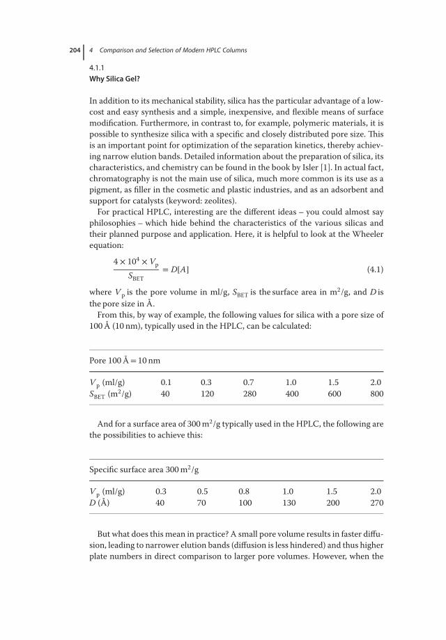
204 4 Comparison and Selection of Modern HPLC Columns

4.1.1Why Silica Gel?

In addition to its mechanical stability, silica has the particular advantage of a low-cost and easy synthesis and a simple, inexpensive, and flexible means of surfacemodification. Furthermore, in contrast to, for example, polymeric materials, it ispossible to synthesize silica with a specific and closely distributed pore size. Thisis an important point for optimization of the separation kinetics, thereby achiev-ing narrow elution bands. Detailed information about the preparation of silica, itscharacteristics, and chemistry can be found in the book by Isler [1]. In actual fact,chromatography is not the main use of silica, much more common is its use as apigment, as filler in the cosmetic and plastic industries, and as an adsorbent andsupport for catalysts (keyword: zeolites).

For practical HPLC, interesting are the different ideas – you could almost sayphilosophies – which hide behind the characteristics of the various silicas andtheir planned purpose and application. Here, it is helpful to look at the Wheelerequation:

4 × 104 × Vp

SBET= D[A] (4.1)

where V p is the pore volume in ml/g, SBET is the surface area in m2/g, and D isthe pore size in Å.

From this, by way of example, the following values for silica with a pore size of100 Å (10 nm), typically used in the HPLC, can be calculated:

Pore 100 Å= 10 nm

V p (ml/g) 0.1 0.3 0.7 1.0 1.5 2.0SBET (m2/g) 40 120 280 400 600 800

And for a surface area of 300 m2/g typically used in the HPLC, the following arethe possibilities to achieve this:

Specific surface area 300 m2/g

V p (ml/g) 0.3 0.5 0.8 1.0 1.5 2.0D (Å) 40 70 100 130 200 270

But what does this mean in practice? A small pore volume results in faster diffu-sion, leading to narrower elution bands (diffusion is less hindered) and thus higherplate numbers in direct comparison to larger pore volumes. However, when the

4.2 Stationary Phases for the HPLC: The Historical Development 205

pore volume is reduced the pore sizes should not at the same time become toosmall, in order to prevent size-exclusion effects on the analytes. The chromato-graphically active specific surface area of the stationary phase is always the mostimportant parameter of the resulting support and, therefore, always the focus ofoptimization during the development of new materials.

A high specific surface area of the stationary phase is desirable as this allowsstronger interaction of the analytes with the stationary phase, often leading tohigher resolution of difficult-to-separate analytes and also counteracting prob-lems with loadability, which manifest themselves in asymmetric and broad elutionbands.

Moreover, it should also be noted that an increase in pore size also leads toreduced mechanical stability, since the structure of the support becomes thin-ner. This is particularly important with materials for UHPLC because there thepressure can reach 1500 bar and the columns are packed at even higher pressures.

Depending on the desired application, different chromatographic supportshave, therefore, been developed. With silica, pore volumes between 0.3 and1.5 ml/g, pore sizes between 60 and 300 Å, and surface areas between 80 and500 m2/g are found. Later, examples are given showing when for which analyteswhich parameters are made use of.

4.2Stationary Phases for the HPLC: The Historical Development

Parallel to the development of silica with respect to purity, stability, and kinetics,the development of the surface modification must also be considered.

As HPLC began, irregular silicas prepared by polymerization of water glass wereused as supports. As a result, depending on how the pH of the solutions wasadjusted and also the origin of the water glass used, the metal content and the pHof the resulting silicas differed considerably. The acidity of the silica in turn has adecisive influence on its reactivity, and thus for modified silicas on their key prop-erties: hydrophobicity, hydrophobic selectivity, silanophilic activity, shape selec-tivity, and polar selectivity.

Irregular silicas were largely replaced in the late 1970s and early 1980s byspherical silicas. The advantage of these supports was primarily their higherpacking density and lower back pressure compared with irregular materials. Adirect result of this is increased mechanical stability and thus a longer lifetimeof the column. Nevertheless, these silicas still had a high and also varying metalcontent, which lead to fluctuations in the properties of the resulting stationaryphase. Stable retention times and uniform separation properties, however, areessential for the use of HPLC in the chemical and pharmaceutical industry.

It still took a few years until in the mid-1980s the first high-purity silicas basedon the polymerization of tetraethoxysilane (TES) were introduced. The metalcontent (mainly Fe and Al) of this support is in the parts per million range. Asa result, it was now possible to comply with the requirements of HPLC quality

206 4 Comparison and Selection of Modern HPLC Columns

control procedures and produce very reproducible separation media. Theseso-called third generation silicas or Type B silicas (as they are often called in theEnglish-speaking countries) now dominate the market for silica.

Nevertheless, the history of supports for HPLC does not stop at this point, andthere are several further developments aimed at either a kinetic optimization ofthe materials (see Chapter 3), an extension of the usable pH range, or the pres-sure stability of the silicas. In the course of kinetic optimization of the materials,essentially the diffusion paths of the analytes interacting with the stationary phaseare shortened. This is done primarily by reducing the particle diameter of the sup-ports.

While at the beginning of the 1990s it was still common to use supportshaving a particle diameter of 5 μm, by the mid-1990s it was quite normal to use3 μm materials from time to time. In the mid-2000s – with the introduction ofUHPLC – sub-2 μm supports came into common use. An important trend in the2010s now aims at the use of materials with nonporous silica cores covered by aporous shell (subsequently referred to as solid core material).

As a result, due to the shorter diffusion paths the separation efficiency of a1.7 μm material can be reached at the back pressure of a 3 μm material. Thesematerials achieve this by the use of a well-known concept developed since the1970s. Even the earliest activities with HPLC used so-called porous layer beads[2, 3]. Admittedly, at that time these materials with particle sizes of about 50 μmwere used as an improvement to the conventional irregular materials (fraction40–63 μm). The disadvantage was the significantly lower loadability (you only hada 1 μm thick porous shell around a 50 μm thick nonporous glass core, which couldnot be compensated for by the advantage of the significantly higher separationefficiency).

With the newer materials, the ratio of core to shell is much better, so that theissue of loadability plays only a minor role. The first solid core materials with par-ticle sizes between 2 and 3 μm clearly aimed at providing an improved alternativeto porous sub-2 μm materials.

In comparison to fully porous sub-2 μm materials, the user has the choicebetween either lower back pressure with the same separation efficiency orsignificantly higher separation efficiency at the same back pressure, as he isable to use longer columns. Since the elution bands of solid core materialsanalog to fully porous sub-2 μm materials are very narrow, then also with thesematerials – despite statements to the contrary in glossy brochures – it is notpossible to use conventional HPLC systems. In order to use the maximumperformance of these columns, it is imperative to optimize the band broadeningoutside the separation column and to use small-volume flow cells and higherdata acquisition rates. Recently, solid core materials with larger particle sizes foruse in the HPLC have been developed. These have particle sizes between 4 and5 μm, are filled in classical HPLC column dimensions, and also show significantlyhigher separation efficiencies as fully porous materials of the same particlesize.

4.2 Stationary Phases for the HPLC: The Historical Development 207

At this point, it should be mentioned that due to the nonporous core, columnsfilled with solid core materials intrinsically have a lower total porosity and hence ahigher packing density. In practice, this means that when comparing a fully porousand a solid core column of the same column dimensions, which are being used atthe same flow (specifically: volume flow), the linear flow rate in the solid core col-umn is higher, and thus a 20–30% higher back pressure is observed compared withthe corresponding fully porous material. If the characteristics of the columns areto be compared in a scientifically correct manner, then measurements must bemade at comparable linear flow rates, that is, the solid core column must be oper-ated at lower flow rates. The linear flow rate is very easy to measure, the columnlength is divided by the hold-up or dead time tM. The hold-up time can be deter-mined from the chromatogram; it is the time at which the disturbance of the baseline, caused by the injection of the sample, often occurs. The solid core columnspacked with 4–5 μm material can be used with conventional HPLC equipment.

In addition to these larger solid core particles, smaller sub-2 μm solid core par-ticles with particle sizes of 1.7 and 1.3 μm are commercially available. However,their theoretical potential with respect to separation efficiency and speed of anal-ysis, which certainly exists, cannot be used in practice. This is because no HPLCsystems are available with the necessary small volumes (of both the capillaries anddetector cells) and which also have the data acquisition rate required to detect andrecord the separations achieved on these columns without loss. Today’s modernUHPLC systems are already quite well optimized, but their performance is by farnot good enough for these applications; the manufacturers face further challengeshere. As with all materials, it is highly recommended to check the batch-to-batchreproducibility especially of solid core phases.

Parallel to the development of particulate materials, there is the possibility ofusing monolithic columns. This technique, developing since the late 1990s, usesthe idea of an inverse silica structure with the same goal: acceleration of the kinet-ics. The biggest advantage of this technique is the very low column back pressure,the separation efficiencies are quite comparable to columns filled with sub-2 μmsupports and the separations are fast [4]. The biggest advantage of monolithiccolumns is the higher total porosity of the material compared with porous silicacolumns. This leads not only to a much lower back pressure, but also to a compar-atively higher column volume. This is exactly the opposite as with the solid corematerials. In practice, this means that monolithic columns show a much largertolerance toward band broadening outside the column and thus high separationefficiencies can be achieved and also measured with conventional HPLC equip-ment without considerable efforts for optimization.

Another advantage is the improved tolerance of these materials toward highlycontaminated samples. These columns do not become contaminated as easily assimilar particulate materials. The disadvantages, however, should also be men-tioned. The columns are limited to a pressure of 200 bar as the monolithic silicarods are seated in a PEEK hull. Furthermore, only a few different selective sta-tionary phases are available. Although recently a few additional bondings such asPhenyl-Hexyl and Cyanopropyl have been announced, only two companies so far

208 4 Comparison and Selection of Modern HPLC Columns

offer these promising columns based on silica. At the moment, however, mono-lithic columns are the most robust and elegant way to achieve fast separations withsufficient separation efficiency (effectively 20 000 plates over a separation distanceof 100 mm).

4.3pH Stability and Restrictions in the Use of Silica

Silicas are the ideal support for stationary phases in the HPLC, as they are mechan-ically stable, can be produced easily and inexpensively and are chemically relativelyinert. As anhydrides of silicic acid, however, they dissolve in alkaline medium. Thisdrawback of silica was taken into account in the history of HPLC and counteractedusing different approaches. The first step was the development of high-purity sil-ica. While the supports of the first generation had a high acidity, due to a highmetal content, the materials of the second generation were significantly purer andthus more pH stable at high pH values. Another approach toward achieving higherpH stability was the coating of the silica with metal oxides such as Al2O3, TiO2,or ZrO2, which reduce the dissolution of the silica at high pH values [5]. A fur-ther possibility is a high surface coverage of the silica-based reversed phases. Withreversed phases having a high surface coverage the dissolution of the silica at highpH values is impeded as the hydrophobic surface is not easily accessible for thepolar bases. Therefore, the higher the surface coverage of the support and thelarger the base used, the more stable is the stationary phase. Other approachesto obtaining increased pH stability are polymeric coatings around the silica andthe introduction of hybrid materials – these are composites of TES and bridgedorganosilanes.

All these approaches lead to a slight improvement in pH stability by aboutone pH unit, but it is falsely suggested to the user that he can always use thesecolumns at pH values greater than 9. This is incorrect! Even as a hybrid materialand coated with polymer, silica is still the anhydride of silicic acid and dissolvesat pH values greater than 7. The rate of dissolution can be reduced by means of ahigh surface coverage of the stationary phase, a coating or an organosilane hybrid.Furthermore, with mobile phases containing a high proportion of aprotic organicsolvents (e.g., acetonitrile), the dissociation of the bases and of the silanol groupsof the silica is suppressed, which in practice leads to much lower pH values.(Careful: up to a pH of about 8, the pH increases after the addition of methanol/acetonitrile [6].) If a stability study of a silica-based HPLC column that reaches10 000 column volumes at pH 12 without loss of efficiency is found in the glossybrochure of a column manufacturer, then this is only possible if the organic sol-vent content is at least 70%, the base very bulky (e.g., triethylamine or pyrrolidine)and the column was used at room temperature. If the same column was used at,for example, 60 ∘C with a small base (ammonia or hydroxide) in mobile phasescontaining less than 10% organic solvent, the service life would be less than 500column volumes. So, care should be taken here!

4.4 The Key Properties of Reversed Phases 209

Must chromatography be performed routinely at a pH above 8, then it may makemore sense to use alternative materials based on polymers, other metal oxidessuch as TiO2, ZrO2, or pure carbon.

There is also the possibility of using a saturation (or conditioning) column. Thisis a tried and tested method of increasing the lifetime of silica-based columns athigh mobile phase pH without using a different support, which could possiblybring selectivity problems. A saturation column is a short column, for example, aguard column, filled with coarse-grained silica. Its particles are slowly dissolved bythe basic mobile phase, which in turn becomes saturated with the dissolved silica,thus sparing the column. Admittedly, it is also possible just to use a column filledwith large particle silica. The saturation column is installed between the pump andinjector, note that this has an effect on the dwell volume of the system.

Why does chromatography at high pH make sense at all? The answer is simple:at a basic pH, basic analytes are present in the unprotonated form. Thus, thehydrophobic interactions between the stationary phase and the analyte arestronger. The ionic interactions are weaker, and as a result the elution bands of thebasic analytes are narrower and more symmetrical than when chromatographedat acidic or neutral pH. Furthermore, since at high pH the basic analytes areno longer ionic, they are more hydrophobic and thus more strongly retainedon reversed phases, which is often very advantageous as it enables movementof the basic components into a different elution window. Moreover, bases in anuncharged state show a significantly higher loadability on reversed phases [7].

Frequently, however, the basic compounds in the uncharged state are signifi-cantly less stable than in the charged state. This is a well-known observation oftennoticed in stability studies. In chromatography, sometimes artifacts are observed,which indicate the decomposition of the products, a fact often kept quiet. There-fore, caution should be exercised when working at high pH. Nevertheless, thevariation of the pH is, alongside the selection of the stationary phase, the mostimportant optimization parameter for the separation of polar or ionic/ionizablecomponents.

4.4The Key Properties of Reversed Phases

The properties that essentially influence the selectivity of the reversed phase arehydrophobicity, hydrophobic selectivity, silanophilic activity, shape selectivity,polar selectivity, and metal content. These properties are different for eachdifferent support and, therefore, essentially determine the separation.

4.4.1The Hydrophobicity of Reversed Phases

The hydrophobicity of the reversed phase indicates how strongly an analyteinteracting primarily via hydrophobic interactions with the stationary phase is

210 4 Comparison and Selection of Modern HPLC Columns

retained. In short, the stronger the retention power of the stationary phase, thehigher the hydrophobicity. The hydrophobicity of a column is determined bythe surface of the support, its carbon content and the surface coverage of thesupport. Phases that have the same hydrophobicity can produce quite differentseparations (even for homologous series!). Therefore, the hydrophobic selectivityshould also be taken into account, which is more important for the separationthan the hydrophobicity itself [8].

4.4.2The Hydrophobic Selectivity

The hydrophobic selectivity is the methylene group selectivity of the stationaryphase, that is, the selectivity of two compounds differing by a methylene group,which are retained predominantly due to their hydrophobicity. This selectivityis to be used, for example, in the case of neutral, hydrophobic analytes for thecomparison of columns and assessment of their similarity, and has a muchhigher significance than the hydrophobicity treated in Section 4.4.1, and latersections.

4.4.3The Silanophilic Activity

Silica has about 9 μmol/m2 silanol groups on its surface [1]. When silica is treatedwith C18-silane, about 3 μmol/m2 of these silanol groups can be made to react,leaving about 6 μmol/m2. Further reactions with shorter chained silanes (usuallytrimethylsilane functionalized silanes) – also known as endcapping – leads to aconversion of about a further 3 μmol/m2 of silanol groups, so that in the finalreversed phase about 3 μmol/m2 of silanol groups remain. These are not con-vertible but can certainly interact with analytes affine to silanol groups, and socontribute to the selectivity of the corresponding reversed phase.

This is the so-called silanophilic activity of the reversed phase. The compoundsaffine to silanol-groups are usually bases that interact with the acidic silanol groupsvia ionic interactions. These interactions are energetically much stronger than theusual hydrophobic interactions of reversed phases, which usually lead to widerelution bands for basic analytes on classical reversed phases.

Therefore, the aim of the manufacturer in the development of new reversedphases is primarily the minimization of the silanophilic activity. This is also themost critical parameter for the reproducible production of reversed phases. Thesilanophilic activity of a reversed phase is determined by the following parame-ters: manufacturing process of the silica, surface coverage of the stationary phase,and type of silane used (reactive and functional groups of the silane).

At this point, however, it should be noted that it is not always desirable to usestationary phases with low silanophilic activity. For example, when no basic com-pounds are present in the sample, then silanol groups may well make a positivecontribution to the selectivity of the stationary phase. Thus, hydrogen bonds are

4.4 The Key Properties of Reversed Phases 211

often observed between silanol groups and carbonyl groups, without which someseparations would not be possible.

4.4.4Shape Selectivity (Molecular Shape Recognition)

Reversed phases also have the ability to differentiate between the spatial configu-rations of analytes in solution, that is, whether analytes are present in a planar orbent form, as is often the case with, for example, cis-, trans-isomers. This prop-erty is called shape selectivity. The parameters of the stationary phase primarilyresponsible for the strength of the shape selectivity of the reversed phase are sur-face coverage of the reversed phase, chain length of the reversed phase, additionalpolar interactions, and pore size of the silica. The following applies:

• The higher the surface coverage, the higher the shape selectivity.• The longer the alkyl chain, the higher the shape selectivity.• The wider the pores, the higher the shape selectivity.• The more additional polar interactions, the higher the shape selectivity.• The lower the temperature and the higher the back pressure of the column, the

higher the shape selectivity.

Why Is This So? The answer is clear. The shape selectivity of a stationary phasedepends crucially on the increased possibility for interactions between the pla-nar analyte and the stationary phase and the simultaneous discrimination againstinteraction of analytes present in the bent form. If the surface coverage is high,then only the more planar molecule together with all its interaction sites can pen-etrate completely into the pores of the stationary phase and consequently be morestrongly retained than the bent molecule.

Analog is the situation when the stationary phase contains longer alkyl chains.Here, the alkyl chains are attracted more strongly to each other, and the moreflexible (longer) they are, the smaller the resulting gaps into which only the pla-nar molecules can penetrate. The same is true if the temperature is lower and thepressure drop higher. The dependence on the pore size is due to the fact that morethan 99% of the chromatographic surface is within the silica particles. If the poresare too small, it is simply impossible to achieve the surface coverage required forsufficient shape selectivity. Therefore, most of the shape selective reversed phaseshave pore sizes larger than 150 Å (15 nm). Here again, of course, exceptions con-firm the rule.

4.4.5The Polar Selectivity

Polar selectivity is generally understood to refer to the differing retention ofpolar analytes relative to neutral analytes in comparison to classical reversed

212 4 Comparison and Selection of Modern HPLC Columns

phases. On polar selective stationary phases, acids are more strongly and basesslightly weaker retained in comparison to classical reversed phases. The polarselectivity is achieved by means of polar groups (amide, carbamate, urea, diol,etc.), which are applied to the surface of the silica and which can undergoadditional interactions with the polar analyte. Polar selective reversed phases arethe first alternative if classical reversed phases do not function, but more on thislater.

4.4.6The Metal Content

The metal content is dependent on the preparation of the silica; the content ishigher or lower depending on the starting material and equipment used. The firstgenerations of silica were prepared from water glass. In these silicas, the metalcontent is relatively high, especially aluminum, and iron are to be found. Butwhy is it so serious if the silica contains metal impurities? Strictly speaking thisshould only cause problems with just a few analytes that are able to interact withthese metals (e.g., complex builders or some proteins). These should undergoadditional interactions with the stationary phase, consequently resulting inbroad unsymmetrical elution bands. However, the metals also influence theacidity of the silica and thus the silanophilic activity (see Section 4.4.3) and,therefore, the reactivity of the silanol groups with the silanes during the surfacemodification.

Even that would not be so bad, if the metal content of the original silica remainsconstant. However, this is not the case. Thus, the batch-to-batch reproducibilityof stationary phases based on non-metal-free silica (the English-speaking litera-ture often addresses Type A silica) is much worse than that of metal-free silica(so-called Type B silica). But here too, some separations require additional metalinteractions and in certain cases it is quite possible that the separation will onlywork on Type A silica. So even today some users still swear on “their” LiChrospher,Select B or Spherisorb ODS 1.

4.5Characterization and Classification of Reversed Phases

Based on the above-mentioned six key properties of reversed phases, the station-ary phases can be characterized. A wide variety of literature exists on this subject[9–15]. Of course, the synthesized stationary phases can be subjected to a fullphysicochemical examination (nitrogen adsorption measurements to determinethe specific surface area, the pore volume and the pore size, CHN analysis to deter-mine the surface coverage of the stationary phase, particle size measurements,etc.). However, all these characterizations are not really to the point, because inthe end only the chromatographic separation counts. As a result, chromatographictests for the characterization and classification of reversed phases have establishedthemselves, from which a representative few, without any claim to being exhaus-tive, are presented here (Figures 4.1–4.3).

4.5 Characterization and Classification of Reversed Phases 213

0 1 2 3 4 5 6 7 8 9 min

0.020.040.06

0.08

0.100.12

0.140.16

0.18AU

1

2

3 45 6

0(a)

(a)

1 2 3 4 5 6 7 8 9 min

0.02

0.04

0.06

0.08

0.10

0.12

0.14AU

1

2

345 6

C18 column with embedded polar groupProntoSIL 120-3-C18 ace-EPS

150 × 4.6 mm

Modern “classical” C18 columnProntoSIL 120-3-C18 H

150 × 4.6 mm

Figure 4.1 Test of polar selectivity: (a,b) neutral (black), acidic (dark gray), and basic (light gray)analytes.

mV

0 1 2 3 4 5 6 7 8 9 10 11 12 13 14 15 16 17 18 19 20 21 22 23 24 25 26 min

0

200

400

600

800

1000

1200

1400

1600

1

2

3

4

56

7 8

0(a)

(b)

1 2 3 4 5 6 7 8 9 10 11 12 13 14 15 16 17 18 19 20 21 22 23 24 25 26 min

0

200

400

600

800

1000

1200

mV

1

2

3

4

56

7 8

Modern “classical” C18 columnProntoSIL 120-3-C18 H

150 × 4.6 mm

C18 column with embedded polar groupProntoSIL 120-3-C18 ace-EPS

150 × 4.6 mm

Figure 4.2 Engelhardt test: (a,b) comparison between classical reversed phase and reversedphase with bedded polar group.

214 4 Comparison and Selection of Modern HPLC Columns

0(a)

(a)

1 2 3 4 5 6 7 8 9 10 11 12 13 14 15 16 17 18 19 20 21 22 23 24 25 26 min

0

200

400

600

800

1000

1200

mV

1

2

3

4

56

7 8

0 1 2 3 4 5 6 7 min

200

400

600

800

1000

1200

1400

1600

mV

1

3

2

4

7

5

8

Fluoro columnProntoSIL 120-5-F-ace

150 × 4.6 mm

Modern “classical” C18 columnProntoSIL 120-3-C18 H

150 × 4.6 mm

Figure 4.3 Neue test: comparison between reversed phase with bedded polar group andfluoro phase.

Test Polar selectivityMobile phase ACN/50 mM Phosphate buffer pH= 3, 65/35 (v/v)Temperature 40 ∘CFlow 1.0 ml/min (column ID 4.0 mm)Detection UV @ 254 nmAnalytes Analyte CharacteristicPeak no. 1 Uracil Dead time markerPeak no. 2 Pyridine Silanophilic activityPeak no. 3 Phenol Polar selectivityPeak no. 4 4-Butylbenzoic acid Polar selectivityPeak no. 5 N,N-Dimethylaniline Silanophilic activityPeak no. 6 Toluene Hydrophobicity

4.5 Characterization and Classification of Reversed Phases 215

Test Engelhardt testMobile phase MeOH/Wasser 49/51 (w/w), respectively, (55/45 (v/v))Temperature 40 ∘CFlow 1.0 ml/min (column ID 4.0 mm)Detection UV @ 254 nmAnalytes Analyte CharacteristicPeak no. 1 Uracil Dead time markerPeak no. 2 Aniline Silanophilic activityPeak no. 3 Phenol Polar selectivityPeak n o. 4 4-Ethylaniline Silanophilic activityPeak no. 5 N,N-Dimethylaniline Silanophilic activityPeak no. 6 Ethyl benzoate Chain length selectivityPeak no. 7 Toluene Hydrophobicity/hydrophobic selectivityPeak no. 8 Ethylbenzene Hydrophobicity/hydrophobic selectivity

Test Neue testMobile phase MeOH/20 mM Phosphate buffer pH= 7, 59.4/40.6 (w/w)

(65/35 (v/v))Temperature 23 ∘CFlow 1.0 ml/min ((bei ID 4.0mm Säulen) column ID 4.0mm)Detection UV @ 210 nmAnalytes Analyte CharacteristicPeak no. 1 Uracil Dead time markerPeak no. 2 Propranolol Silanophilic activityPeak no. 3 Butylparabene Polar selectivityPeak no. 4 Dipropylphthalate Polar selectivityPeak no. 5 Naphthalene HydrophobicityPeak no. 6 Amitriptyline Silanophilic activityPeak no. 7 Acenaphthene Hydrophobicity

It should also be mentioned that the characteristics of the columns change withuse, depending on the buffer, additive, and also the sample matrix. In practice, thishas several consequences:

• During method development and optimization, HPLC columns “see” severalmobile phases of differing pH and containing different buffers, as well as addi-tives. If you have reached the end of a method optimization, then it is best to

216 4 Comparison and Selection of Modern HPLC Columns

characterize the column using a chromatographic test. This allows you to iden-tify any subsequent variations and quickly find alternative solutions. We discussthis topic in more detail later under the heading of column databases.

• During HPLC method validation, it is imperative to test the finished optimizedmethod on several (usually three) new columns from different productionbatches in order to see whether the separation still functions. If this is the case,you can be hopeful that future batches will work. Sometimes, it is necessary,however, to precondition the columns by means of a defined conditioningprogram before they meet the requirements of the separation. This is thereason why the verification of the selectivity is so important.

4.5.1The Significance of Retention and Selectivity Factors in Column Tests

4.5.1.1 Preliminary RemarkThe hydrophobicity of a stationary phase is responsible for the retention ofthe analytes. This is mainly determined by the specific surface area and thecarbon content, discussed earlier. But as far as the selectivity is concerned, inreversed-phase (RP)-chromatography hydrophobic interactions usually play amuch less important role than is generally believed, ionic/polar interactions,and steric aspects – if they come into play – are more dominant factors. Onlyby means of these influencing factors can analytes be differentiated. This is alsothe reason why a correlation between retention and selectivity factors is ratherseldom observed, discussed later. Such a correlation may at the best be expectedfrom a uniform RP mechanism in which van der Waals interactions predominate,which is seldom the case (homologous series or simple pairs of analytes suchas toluene/ethyl benzene). This is because the molecules to be analyzed mostlyhave groups that are capable of ionic/polar interactions. Even with hydrophobicaromatic compounds, we are dealing with induced dipoles; in addition, thepolarity may increase through resonance.

Otherwise, “similar” molecules also differ in their spatial dimensions; their stericproperties influence their diffusion behavior in the pores of the phase surface.Examples here are the polarizability of molecules due to double bonds, or theirrigidity/flexibility depending on the location of substituents on the aromatic ring.

In conclusion: in an RP-system hydrophobic interactions are primarily respon-sible for the retention, in the case of ionic analytes naturally also ion exchangewhen this is possible. On the other hand, polar/ionic interactions are decisive forthe selectivity. These are primarily ion exchange as well as hydrogen bonding anddipole-dipole interactions, possibly even complex forming/chelation.

4.5.1.2 Criteria for the Comparison of ColumnsIn the literature, the hydrophobicity is often used as a criterion for comparison ofstationary phases. For this purpose, ln k values (k = retention factor) of typical RPanalytes on different stationary phases are compared, on “similar” hydrophobicphases the analyte will be equally strongly retained, leading to similar ln k val-ues. This practice should be critically questioned. Without going into details about

4.5 Characterization and Classification of Reversed Phases 217

the suitability of the (usually simple) analytes used, the fundamental question ofwhether, if at all, retention factors represent a suitable criterion for comparisonshould be dealt with.

From a practical perspective, the retention behavior (a measure of thehydrophobicity) is only of fringe interest. The reason is that in comparative teststhe user is more interested in finding columns that show similarly good separationfor certain analytes rather than in finding columns on which the analytes eluteafter a similar retention time. And a measure of the separating efficiency happensto be the selectivity (separation factor, 𝛼). Similarly, strong interactions – andthus similar retention factors – do not at all mean that the respective phases alsoshow similar selectivity.

This has been repeatedly confirmed in several studies; see, for example,Figure 4.4. Here, the retention (bars) and separation factors (lines) of tricyclicantidepressants in acidic acetonitrile/phosphate buffer are shown. In the case ofquite different retention factors depending on the hydrophobic character of thephases (differently strong interactions), apart from a few exceptions very similarseparation factors result. Although the analytes are retained for different lengthsof time on the stationary phases, they show a similar selectivity behavior. This isobserved especially with neutral or – by means of the pH-neutralized molecules.In this case, mainly hydrophobic interactions between the analytes and thesurface of the material dominate. These are not especially specific; the individualdifferences of the phases with respect to selectivity do not come into effect.

Figure 4.5 illustrates this phenomenon for the separation of ketones, polarbut nonionizable analytes. Moreover, a strong interaction does not automat-ically mean good selectivity – see also Figure 4.6, in which, in principle, thisphenomenon is presented slightly differently. There, retention factors on variouscolumns are plotted against the corresponding separation factors. The fact isthat the peaks elute early or late on the different columns (according to “Hy-drophobicity” these are phases with different properties) but the selectivity ofthese columns is very similar – all 𝛼 values lie between about 𝛼 = 1.1–1.2. For aseparation technique such as HPLC, selectivity should be the most important ormost meaningful criterion when it comes to assessing the similarity of RP phases.

To verify this assumption, several chemometric analyses (with strongly differingseparation conditions and analytes) were performed and extensive data collected.Figure 4.7 shows an example of these studies. The farther apart the variables (hereretention and separation factors) are located around the origin on the y-axis, thegreater their influence on the differentiation of objects, here columns. As can eas-ily be seen, the 𝛼-values are suitable for this. If nevertheless k-values must beused, then at the most “problem” substances are suitable. For example, polar ana-lytes in unbuffered eluent (e.g., k Cos, caffeine) or strong acids in buffered eluents(k Phs, phthalic acid, and k Tes, terephthalic acid) because the differences betweenthe phases only become visible when polar (ionic) interactions are possible. This,however, is not the case when only hydrophobic interactions are expected; theissue of “column comparison” and thus “column selection” is then not so critical,any “good” column can be used and for logical reasons optimization is more easily

218 4 Comparison and Selection of Modern HPLC Columns

12.00k Amik Triα

1.40

1.30

1.20

1.10

1.00

0.90

0.80

0.70

0.60

0.50

10.00

8.00

6.00

4.00

2.00P

latin

um

EP

S

VY

DA

C

Bo

nd

ap

ak

LiC

hro

so

rb

LiC

hro

sh

er

Se

lect

B

LiC

hro

sp

he

r

Pla

tin

um

C1

8

Gro

msil

AB

Su

pe

rsp

he

r

Su

pe

rsp

he

r S

ele

ct

B

Su

pe

riso

rb O

DS

1

Su

pe

rso

rb O

DS

2

Ultra

se

p E

S

Flu

ofix I

NW

Ine

rtsil

OD

S 3

To

so

Ha

as T

SK

Hyp

ers

il E

lite

Hyp

ers

il O

DS

Ju

pite

r

Su

pe

lco

sil

AB

Z p

lus

Re

pro

-Sil

AQ

Dis

co

ve

ry C

18

Dis

co

ve

ry C

16

Nu

cle

osil

HD

Nu

cle

osil

10

0

Nu

cle

osil

Pro

tect

1

Zo

rba

x O

DS

Nu

cle

osil

50

Pu

rosp

he

r

MP

-Ge

l

Re

pro

-Sil

OD

S

Pro

nto

sil

AQ

Ine

rtsil

OD

S 2

Pro

nto

sil

C1

8

Hyp

ers

il B

DS

YM

C C

18

YM

C A

Q

Pro

dig

y

Flu

ofix I

EW

No

va

-Pa

k

Lu

na

Zo

rba

x S

B C

18

Zo

rba

x S

B C

8

SM

T

Gro

msil

CP

Sym

me

try

Kro

ma

sil

Nu

cle

osil

AB

0.00

Figure 4.4 Charakterization of different RP stationary phases. Reproduced from Kromidas [6], with permission of Wiley.

4.5 Characterization and Classification of Reversed Phases 219

5.00 3.00k lsoprok lsobuα 2.50

2.00

1.50

1.00

0.50

0.00

4.50

4.00

3.50

3.00

2.50

2.00

1.50

1.00

0.50

0.00

Aqua

Zorb

ax E

xte

nd

Sym

metr

y S

hie

ld C

18

Zorb

ax B

onus R

P

Nucle

osil

HD

Pro

nto

Sil

AC

E

XT

err

a M

S

XT

err

a

Chro

molit

hP

erf

orm

ance

Puro

spher

Sta

r

Nucle

osil

Nautitlus

HyP

UR

ITY

Advance

LiC

hro

sorb

Pla

tinum

E

PS

Figure 4.5 Hydrophobicity and Methylen group selectivity. Reproduced from Kromidas [6],with permission of John Wiley & Sons.

10.00

9.00

8.00

7.00

6.00

5.00

4.00

3.00

2.00

1.00

0.000.50 1.00 1.50

α Desmeth–Nortr

k D

esm

eth

2.00 2.50 3.00

Figure 4.6 On the bandwith of retention and separation factors by the separation ofmetabolites of tricyclic anti-depressants in acetonitrile/acidic phosphate buffer. Reproducedfrom Kromidas [6] with permission of John Wiley & Sons.

220 4 Comparison and Selection of Modern HPLC Columns

Figure 4.7 On the suitability of k- and 𝛼-values for a differentiation of stationary phases; forcomments, see text. Reproduced from Kromidas [6] with permission of John Wiley & Sons.

done with the eluent. Nevertheless, having the optimal column that can be used incombination with an easy mobile phase makes chromatography in general morerobust and better transferable from one lab to another. Therefore, finding the opti-mal column for our separation task should be our first predominant focus duringmethod development.

4.5.2Column Comparison, Comparison Criteria: Similarity of Selectivities

A comprehensive review of diversified tests and visualization tools for the com-parison of columns is available in Ref. [8]. In the following, we present three teststhat appear to us to be quite informative. For the reasons set out earlier, the selec-tivity (separation factor) is used as the classification criterion for comparison ofcolumns.

1) Selectivity plotsHere, separation factors, determined by means of separations on supposedlysimilar phases under defined chromatographic conditions, are plotted againsteach other. The more similar the phases, the closer to the resulting diago-nal the individual values should lie. In a series of experiments, 68 differentpairs of analytes were separated under deliberately varying chromatographicconditions (nine different eluents) and the resulting 𝛼-values plotted against

4.5 Characterization and Classification of Reversed Phases 221

4.00

3.50

3.00

8 5553

423

572555430

2433

56

58157459

466126

28

40

3947

9

4138

34

18

3651

6

852

17

22

31

16

2129

19

37

1

35

3243

60

2.50

Kro

ma

sil

2.00

1.50

1.00

1.00 1.50 2.00 2.50

Luna

3.00 3.50 4.00

Kromasil

Figure 4.8 Plot of the separation factors of analyte pairs that differ as much as possible, ontwo columns; for explanation see text.

each other. Due to the large number of values and the different experimentalconditions, quite substantiated assertions can be made regarding the similar-ity of the phases. An example of such a plot is shown in Figure 4.8, in whichtwo C18 columns, Kromasil and LUNA (2), are compared.From Figure 4.8, first, it can be seen that both columns have a similar charac-ter. This is to be expected, as both columns are hydrophobic endcapped C18phases with a classical high surface coverage and based on high-purity silica.What is striking is the outlier “21.” The 𝛼-value corresponds to the separationof 2,2′-/4,4′-bipyridine after the column has been in use for 4 weeks. A large𝛼-value is an indication of the presence of heavy metal ions in the silica matrix,as 2,2′-bipyridine builds complexes, whereas 4,4′ does not. Apparently, duringuse of the column more metal ions accumulate on the silica surface of Kro-masil, and the tendency to complex formation increases. As both silicas areoriginally ultrapure, the metal stems either from the frit on the column inletor from the eluent and is enriched in the column since silica-based columnsare always cation exchangers. Otherwise, this batch of silica from Kromasilcontains traces of metal ions that are missing from LUNA. Furthermore, withLUNA, the slightly higher hydrophobic character is apparent; see separation“37,” the separation of 3-hydroxy/4-hydroxybenzoic acid, two weak acids. Infact, LUNA does have a slightly higher degree of coverage compared with Kro-masil; the phase has a slightly greater hydrophobic selectivity.With such plots, it can be determined whether two supposedly similarcolumns do indeed have a similar selectivity performance for this analyte.Also, with this method the batch-to-batch reproducibility of a materialcan be tested, or whether during routine use this sample matrix and/or

222 4 Comparison and Selection of Modern HPLC Columns

UptisphereUP5MM1

GeminiC18

XBridge

a Phenol/Toluol

0

6.00

5.00

4.00

a P

henol/E

thylb

enzol

3.00

2.00

1.00

0.00

1 2 3 4 5 6 7 8 9

Figure 4.9 Plot of the separation factors of two characteristic analyte pairs on severalcolumns; for explanation see text.

these chromatographic conditions have caused (irreversible) changes to thecharacter of a certain column.

2) Plot of the separation factors of two very similar analyte pairs, obtained onthe columns to be compared, for example, phenol/ethyl benzene and phe-nol/toluene.Since these molecules are typical, simple RP analytes and are also very similar(a difference of only one methylene group between toluene and ethylbenzene),separation on different phases with similar selectivity factors should be possi-ble. Only phases with “really” different characters should be “out of line” here.The three outliers in Figure 4.9 do in fact represent exceptions: Gemini andXBridge are hybrid materials, and Uptisphere UP 5MM1 is the only phasewith a phenyl and a cyclopentenyl group as end groups. With this test, it can,for example, be tested which column(s) show an entirely different selectivityfor which analyte. From the results, suitable candidates for orthogonal testscan also be determined.

3) Plot of the separation factors of two analyte pairs of interest on differentcolumnsAnalyte pairs that reveal the similarity of the phases with respect to selec-tivity for the current issues should be chosen. Assume that in one case theseparation of both simple neutral molecules as well as aromatics is relevant;see Figure 4.10. Ethylbenzene/fluorenone is a measure for the hydrophobicselectivity and chrysene/perylene for the aromatic selectivity. XTerra MSand AQUA as quite hydrophobic phases show good hydrophobic selectivity,

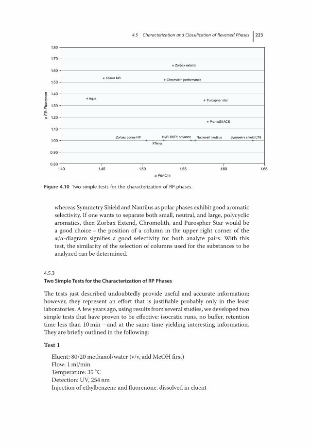
4.5 Characterization and Classification of Reversed Phases 223

1.80

1.70

XTerra MS

Aqua

Zorbax extend

Chromolith performance

Purospher star

ProntoSil ACE

Zorbax bonus RP

XTerra

HyPURITY advance Nucleosil nautilus Symmetry shield C18

1.60

1.50

1.40

a E

B-F

luo

ren

on

1.30

1.20

1.10

1.00

0.90

0.80

1.40 1.45 1.50 1.55

a Per-Chr

1.60 1.65

Figure 4.10 Two simple tests for the characterization of RP-phases.

whereas Symmetry Shield and Nautilus as polar phases exhibit good aromaticselectivity. If one wants to separate both small, neutral, and large, polycyclicaromatics, then Zorbax Extend, Chromolith, and Purospher Star would bea good choice – the position of a column in the upper right corner of the𝛼/𝛼-diagram signifies a good selectivity for both analyte pairs. With thistest, the similarity of the selection of columns used for the substances to beanalyzed can be determined.

4.5.3Two Simple Tests for the Characterization of RP Phases

The tests just described undoubtedly provide useful and accurate information;however, they represent an effort that is justifiable probably only in the leastlaboratories. A few years ago, using results from several studies, we developed twosimple tests that have proven to be effective: isocratic runs, no buffer, retentiontime less than 10 min – and at the same time yielding interesting information.They are briefly outlined in the following:

Test 1

Eluent: 80/20 methanol/water (v/v, add MeOH first)Flow: 1 ml/minTemperature: 35 ∘CDetection: UV, 254 nmInjection of ethylbenzene and fluorenone, dissolved in eluent

224 4 Comparison and Selection of Modern HPLC Columns

Test 2

Eluent: 40/60 methanol/water (v/v, add MeOH first)Remaining, as described in Test 1Injection of phenol and benzylamine dissolved in eluent (freshly prepared solu-

tions)Results and comments

4.5.3.1 Test 1If a column shows a separation factor greater than 1.4 then it is a phase with highhydrophobic selectivity, a separation factor greater than 1.6 indicates a phase witha very high hydrophobic selectivity. Phases with high hydrophobic selectivity aresuitable for the separation of small monocyclic aromatics, for homologs with a dif-ference in the alkyl chain, for aldehydes, ketones, esters, and for neutral “unprob-lematic” analytes such as weak organic bases and weak organic acids. Columnsthat only show small separation factors in this test are suitable for the separationof smaller polar impurities and twisted structures, as well as carotenoids, steroids,double bond isomers, polycyclic aromatics, and analytes present in ionic formsuch as strong acids or in general any analytes having polar character, such asphospholipids and dyes.

4.5.3.2 Test 2The later benzylamine elutes compared with phenol, the stronger the polar char-acter of the phase (more precisely: it has groups that are able to undergo ionicinteractions). An elution close to phenol or co-elution indicates a hydrophobicphase, elution even before phenol a very well coated, very hydrophobic RP phaseor a stationary phase where interactions with silanol groups are suppressed bypolar functional groups such as amide or other nitrogen-containing groups. Ifsuch a phase shows the desired selectivity for the current issue, then serious prob-lems with this column are hardly to be expected in routine use, it offers goodsymmetrical peak shape, reproducible retention times, and long life.

4.6Procedure for Practical Method Development

The selection of the column is of crucial importance and, therefore, has the utmostpriority in any method development. In this chapter, a guide is given to the strategyby which it should be possible to rapidly find the most appropriate column. But,before we come to the list, first some important rules – these are often ignoredbut, when complied with, lead sooner to success.

4.6.1The Interaction between Mobile and Stationary Phase

The separation results from the combination of mobile and stationary phases (andof course temperature). Some combinations are not practicable and, therefore,

4.6 Procedure for Practical Method Development 225

either cannot be considered at all, or only (almost in despair) when all other com-binations do not work.

The following is the most important basic principle here:For the chromatography of basic compounds on nonpolar stationary phases

(classical reversed phase), use preferably aprotic solvents (e.g., acetonitrile) as themobile phase and on polar stationary phases (reversed phase with embedded polargroups) preferably protic solvents (e.g., methanol).

4.6.1.1 Why Is This?

Protic solvents solvate polar functional groups and thereby make them moreexposed. The only polar functional groups that can be found on a conventionalnonpolar reversed phase are the silanol groups. If these are made more prominentby solvation, then the undesired ionic interactions with basic analytes come moreto the fore and the elution bands become broad and asymmetric. If, however,an aprotic solvent such as acetonitrile is used with these columns, then the lonepair electrons of acetonitrile can form hydrogen bonds with the silanol groups,and these will be shielded from the basic analytes. The elution bands are muchnarrower and more symmetrical.

With polar reversed phases, the effect is exactly the opposite. Here, the polargroups (usually nitrogen-containing functional groups) become exposed by theuse of protic solvents and thereby interact with the silanol groups. This has theadvantage that then the basic analyte cannot interact with these silanol groups.As a result, when protic solvents are used bases elute from polar reversed phaseswith symmetrical elution bands.

When acidic analytes are being separated, for maximum selectivity the strongestpossible interactions of the analytes with the silanol groups of the stationary phaseare required. Consequently, in this case it makes sense with classical, nonpolarstationary phases to use protic solvents such as methanol as the mobile phase.With polar stationary phases the polar interactions should be suppressed as muchas possible, and so here aprotic solvents such as acetonitrile should be used as themobile phase.

When both acids and bases are present in a sample, then mobile phases suitablefor the bases are normally used, as broad and asymmetric elution bands generallyhave a more serious effect on the analytical problem as a slightly inferior selectivity.In such cases, as a compromise mixtures of protic and aprotic solvents (methanoland acetonitrile) are sometimes used.

Furthermore, in the reversed-phase HPLC stationary phases whose surface hasbeen modified with phenyl or pentafluorophenyl groups are also used. These func-tional groups can only develop their maximum selectivity when they are solvated.Therefore, with these columns it is imperative to use a protic solvent as mobilephase. The use of acetonitrile is ruled out, since its lone-pair electrons interactwith the stationary phase and thus the interaction of the phenyl groups with theanalyte is at least suppressed, if not completely blocked.

When these few rules are followed, then success comes rapidly.

226 4 Comparison and Selection of Modern HPLC Columns

4.6.2Which Columns Should Be Used, and How Do I Use Them?

First of all, we need to distinguish between whether all the analytes to be deter-mined and all the analytical issues are known, or if there is the possibility thatunknown impurities are present.

When our analytes and our analytical goal are known, then we can select thecolumn directed toward this aim. If, for example, we want to separate organicacids differing primarily in the chain length of the aliphatic rest, that is, in theirhydrophobic selectivity, then it is best to try a classical endcapped, hydrophobicreversed phase, because this provides the methylene selectivity necessary for thisproblem.

If, on the other hand, we want to separate aromatic carboxylic acids, which differin the position of the functional groups on the aromatic ring, then to start with aclassical reversed phase would not promise much success. Here, the analytes differmainly in their 𝜋-electron density on the aromatic ring and such analytes can beseparated most effectively via 𝜋–𝜋 interactions. Thus, in this case the use of astationary phase with phenyl groups would be the first choice. As mentioned inChapter 3, in HPLC the separation and thus the resolution are primarily achievedthrough the selectivity, and this in turn depends strongly among other things onuse of the correct column.

So if we have information on the analytes to be separated, then we can use thisfor clever selection of the column to be used.

If we have to clarify the heterogeneity of an unknown sample, the sample mustbe examined on various columns with orthogonal selectivity to ensure that a pos-sible co-elution is not overlooked. Selection of these columns is best orientatedon the key characteristics of the columns, which were considered in Section 4.4.

Therefore, a modern C18 or C8 column with a good efficient endcapping shouldbe tried first. In the most cases this will be successful. Two typical examples herewould be Chromolith High Resolution RP 18e from Merck and YMC Pro C8.The Chromolith column has the advantage of high separation efficiency at rela-tively low back pressure and at the same time shorter column length. Due to theirchromatographic performance, C8 columns are to be preferred to C18 columnsas they usually have a higher surface coverage and, therefore, fewer unwanted sec-ondary interactions between bases and the stationary phase are possible. However,if strong methylene group selectivity is required (i.e., two large molecules that dif-fer in just one methylene group need to be separated) a C18 is always superiorcompared with a C8 stationary phase. If somewhat stronger bases are expected inour sample, a particulate C8 column is preferable to the monolithic C18 column.The retention on a monolithic C8 column would be too weak and it is, therefore,not really suitable for general use, in special cases, however, it is definitely an alter-native.

If the separation does not work on a classical reversed phase, then the type ofstationary phase must be radically changed. A change to a classical packing from adifferent manufacturer is only successful in isolated cases. The column with which

4.6 Procedure for Practical Method Development 227

one has the most success after the classical packing is a reversed phase with anembedded polar group. As typical representatives, ProntoSIL C18 ace-EPS fromBischoff or Symmetry Shield RP 18 from Waters could be named here. Theseshow similar hydrophobic retention to classical reversed phases (most reversedphases with bonded polar groups are weakly retentive) and have a fairly high polarselectivity.

If even this column does not give the desired separation, the next choice wouldbe a phenyl column. Examples of this column type are XSelect CSH Phenyl-Hexylfrom Waters or Zorbax Phenyl from Agilent Technologies. Many manufacturersuse hexyl as a spacer for the phenyl group. With increasing chain length thestrength of the 𝜋–𝜋 interactions increases [16]. Recently, Restek introduced abiphenyl-bonded stationary phase, which provides slightly different selectivitycompared with traditional phenyl columns.

And if even this column does not work, then a classical reversed phase withhigh metal content and without endcapping or a modern non-endcapped C30column with high shape selectivity would be the column of choice. Recommenda-tions from this category are LiChrospher RP 18 from Merck or ProntoSIL 200 C30from Bischoff. At this point, a practical tip to shape selectivity: the shape selectivityis strongly temperature dependent; the lower the column temperature, the higherthe shape selectivity. Therefore, “shape”-selective separations should best be doneat low temperatures. The same effect as lowering the temperature can be observedby increasing the back pressure of the column. This can be achieved either by usingsmaller particle diameters or a restriction capillary after the column. This effect isobserved at back pressures of 500 bar and higher.

A further option would be the use of a cyano (CN) column. A typical classi-cal CN column would be Nucleosil CN from Macherey Nagel or LUNA CN fromPhenomenex. These columns separate via dipole interactions and thus preferen-tially compounds that differ in their dipole moment. Due to their low hydrophobicselectivity, however, with these columns, it often comes to co-elution of com-pounds having similar dipole moments and only slightly differing hydrophobicity.Nevertheless, these columns offer an interesting alternative for group separations,which then show their strengths in combination with 2D-LC or phase-optimizedliquid chromatography (POPLC).

Very hydrophobic analytes often interact very strongly with the stationary phaseand are sometimes not eluted from conventional reversed phases. Here, the use ofa very short chain alkyl phase modified only with trimethylsilane groups helps. Awell-proven column here is Zorbax TMS from Agilent Technologies. Other man-ufacturers also offer this kind of column and call them C1, RP2, or SAS.

During selection of these columns, it may happen that on some columns twocomponents are separated, but other components that are separated on othercolumns suddenly coincide. In such cases, POPLC can be used [17, 18]. The prin-ciple is shown in Figure 4.11. A set of segmented columns is contained in a columnkit. This set represents the columns of differing selectivity described earlier. Froman initial measurement on the individual columns, the retention time of each

228 4 Comparison and Selection of Modern HPLC Columns

Sample

Initial runs, up to fivedifferent bonded phases

Column optimized to sample

1

1

23

45 6

78

1

1

2&3

2&3

2&3

4&5

4&5

5&6

4

23

67

ProntoSIL C18H

ProntoSIL C18-EPS

ProntoSIL Phenyl

ProntoSIL CN

ProntoSIL C30

7

76

1 456

7 8

4&5

1

23

67 8

8

8

8 O

ptimizer

So f t w a r e

Figure 4.11 POPLC scheme.

4.6 Procedure for Practical Method Development 229

compound is determined and by means of a software program the ideal compo-sition of the separation column determined. Through objective-based couplingPOPLC can deliver the “best” column composition for the current separation.However, when the number of analytes to be separated exceeds about 20, thenusually POPLC optimization does not give a solution either. Here, only high peakcapacity (i.e., 2-D HPLC) or a high plate number can help.

4.6.3What to Do, When the Analytes Are Very Polar and Are not Retained on theabove-Mentioned Columns?

Polar analytes are very often a major challenge to reversed-phase chromatography.This is because even with very polar (completely aqueous) mobile phases only littleor no retention can be achieved. For these cases, there are certain strategies thatare discussed in the following.

4.6.3.1 AQ Columns, Polar RP Columns, and Ion-Pair ChromatographyIf polar analytes are to be separated with reversed-phase HPLC, then very polarmobile phases must be used. An increase in the water content of the mobile phaseleads to an increase in retention. With classical reversed phases, this is the case (atleast for pressures under 200 bar) only when the proportion of organic solvent isabove 5%. Below this, the retention suddenly collapses, so classical C18 columnscannot be used with 100% aqueous eluents. This is due to the high surface ten-sion of water. More than 99% of the specific surface area of the stationary phase islocated in the pores. If the proportion of organic solvent in the mobile phase fallsbelow 5%, a “drop” forms at the entrance to the pores, which prevents the move-ment of analytes into and out of the pores. Only when the pressure rises above200 bar is this again possible [7].

As a result, stationary phases have been developed that allow the reversed-phasemode to be used in purely aqueous media. These include so-called AQ columns,which often have AQ in their name or are called aqua or hydro. Sometimes, theirnames are only associated with water, such as Atlantis. In principle, the water com-patibility can be achieved in three ways:

a) Lower surface coverage. For example, Platinum EPS from Alltech or AtlantisT3 from Waters. These columns are classical C18 columns but have a signifi-cantly lower surface coverage than conventional C18 columns. They often havea conventional endcapping (Platinum EPS does not) and also exhibit the selec-tivity of conventional columns. Due to the low surface coverage, however, abetter accessibility of the surface is achieved; residual polar silanol groups canbe “seen” and solvated and thereby the pore accessibility is maintained.

b) Polar endcapping, for example, Aquasil C18 from Thermo or ReproSIL C18 AQfrom Dr Maisch. With these stationary phases, endcapping is achieved with asmall silane containing a polar group instead of conventional endcapping withtrimethylsilane groups. This ensures the wetting of the surface and, therefore,the accessibility of the pores.

230 4 Comparison and Selection of Modern HPLC Columns

c) Reversed phases with an embedded polar group, for example, Ascentis RPAmide from Sigma Aldrich or XBridge Shield RP18 from Waters. Thesestationary phases have a polar group (amide, carbamate, or urea) incorpo-rated into the alkyl chain. The endcapping of these materials is conventional(trimethylsilane groups). With these columns the polar group built into thealkyl chain ensures the surface wetting.

Finally, other highly polar phases can be thought of such as various fluorinatedphases, Zorbax Bonus RP, or Synergi POLAR RP.

An unusual but repeatedly successful measure is a typical RP eluent (e.g.,buffer/ACN) plus silica. This is the “aqueous normal phase” chromatographyknown from the 1980s (in the gradient mode nowadays known as hydrophobicinteraction liquid chromatography (HILIC), discussed later).

If the analytes to be separated are so polar that even 100% aqueous mobilephases are not sufficient to retain them on the above-mentioned columns, thenat least for ionizable analytes ion-pair chromatography helps. In ion-pair chro-matography, reagents of opposite charge to the sample and which contain a polargroup and a nonpolar residue are added to the mobile phase. These additionalanionic or cationic surfactants then form together with the polar cationic oranionic analytes a so-called ion pair, which is then outwardly electrically neutraland can be retained on reversed phases. Other conceptions assume that thesurface of the stationary phase becomes coated with the corresponding ion-pairreagent and so an ion exchanger is present, on which it is then possible to separatethe oppositely charged analyte ions. The truth probably lies between these twomodels. Ion-pair chromatography is a very elegant means to chromatographionic analytes in reversed phase mode; however, in practice some points have tobe considered.

a) Equilibration of an ion-pair reagent with the stationary phase takes a long time,the column should be equilibrated overnight at a low flow. AQ columns are themost suitable for use in ion-pair chromatography as they allow good access tothe complete chromatographic surface and are normally equilibrated twice asfast as conventional C18 columns (this is also true for the customary use ofthese columns in nonpolar applications).

b) When using an ion-pair reagent, care must be taken to ensure that at all timesboth the analyte and the ion-pair reagent are present in dissociated form.Therefore, appropriate buffering of the eluent is necessary.

c) Ion-pair reagents are also always surfactants and so difficult to obtain com-mercially in ultrapure form. As a result, the ion-pair reagents often containimpurities, which in the case of gradient elution are initially enriched at thehead of the column, elute with increasing solvent strength, and then appearin the chromatogram as so-called “ghost peaks.” This is not serious when noco-elution with the analyte to be measured occurs. However, it is necessaryto locate and know the ghost peaks in the chromatogram. Therefore, a blindinjection () must be made before the actual chromatographic run and also theequilibrium time between the individual chromatographic runs must remain

4.6 Procedure for Practical Method Development 231

constant, as otherwise after prolonged equilibration the intensity of the “ghostpeaks” changes.

d) From experience, for the separation of anions the purest ion-pair reagentis tetrabutylammonium hydrogen sulfate (TBAHSO4), for the separation ofcations sodium dodecyl sulfate (SDS). Typical concentrations used in theeluent are 10 mM ion-pair reagent and 20 mM buffer. However, it is alwaysworth varying the ion-pair concentration during method development toexamine the influence on peak shape and selectivity and, therefore, robustnessof the method.

e) As ion-pair reagents are not volatile, mass spectrometric and aerosol detectorscannot be used. It is, however, possible by means of suppressors before thedetector to free the eluate from the ion-pair reagents; these detectors can thenbe used [19].

Another elegant way to avoid ion-pair chromatography is the use of so-called“mixed-mode” columns.

4.6.3.2 Mixed-Mode Columns

Mixed-mode columns contain reversed as well as various other functionalgroups, for example, often groups capable of forming complexes or ion-exchangegroups. Because here the interaction-capable groups are bonded covalentlyto the stationary phase, these materials provide an elegant way of retainingionizable polar analytes without the addition of ion-pair reagents. When usingmixed-mode columns, volatile buffers can be added to the mobile phase, allowingthe use of aerosol and mass spectrometric detectors. There are some columnmanufacturers who have specialized in mixed-mode columns. Frequently usedmixed-mode columns are the Primesep columns from Sielc. These are obtainableas strong cation exchanger (Primesep 100), weak cation exchanger (Primesep200), strong anion exchanger (Primesep B), and weak anion exchanger (PrimesepB2), so that the corresponding column for each analytical application is available.A column with a complex-capable group on the alkyl residue would be PrimesepC. Further examples of mixed-mode columns are Acclaim Mixed-Mode HILIC 1,Scherzo SM-C18, and Obelisc R or N.

Other columns with multiple ion-exchange groups and an additional het-eroatom such as sulfur appear to us to be too special and are not furtherconsidered here. The special practical charm of these columns lies in the fact thatby increasing the acetonitrile content during the gradient not only the solventstrength for the RP retention mechanism is increased, but at the same time theprotolysis equilibrium of the ion-exchangeable groups is suppressed, resulting inthe elution of ionic analytes.

In fact, every silica-based reversed phase represents a mixed-mode column,because besides the alkyl chains it has silanol groups, which are groups capa-ble of weak cation exchange. Some C18 materials of the first generation, such asPartisil ODS from Whatman or Spherisorb ODS1 from Waters, have only a verylow carbon content (<5%) and a high number of free silanol groups. With these

232 4 Comparison and Selection of Modern HPLC Columns

columns, strongly basic compounds can be separated and elute with symmetri-cal peak shapes. This is because in these stationary phases the silanol groups arepresent in such a large number that they are not overloaded and, therefore, sym-metrical elution bands result.

In the earlier sections, we have discussed the options available to retain ionizablepolar analytes. In the following, we show possibilities to retain and chromatographneutral and ionizable analytes together.

4.6.3.3 Ion-Exchange Columns/Ligand-Exchange Chromatography

These materials are polymer-based stationary phases, more exactly exhaustivelysulfonated polystyrene-divinylbenzene copolymers. The retention mechanism ofthese separations is very complex and is often founded on the possibility for theanalytes to undergo interactions similar to ligand complexes with the cation of thestationary phase [20]. However, the separations often work very well especially forpolar analytes containing many hydroxyl groups, such as sugar. The mobile phaseused in this case is slightly acidic water. These columns are available not only inthe acidic H+ form but also containing various metals (Ca2+ and Pb2+), resulting invarying selectivities. For the separation of sugars, primarily the metal-containingcolumns are used, while for the separation of organic acids the use of the H+ formis preferred. These columns are available from many manufacturers. As a provencolumn, Shodex K-801 is mentioned. These stationary phases generally have smallpores. To accelerate the mass transfer, it is recommended to run the columns atelevated temperatures such as 60–80 ∘C.

4.6.3.4 HILIC (Hydrophilic Interaction Liquid Chromatography)

In the case of HILIC, polar stationary phases are used with mobile phases con-sisting of at least one polar and one nonpolar solvent. Usually, these are acetoni-trile/water mixtures with a high proportion of acetonitrile. HILIC is, therefore,an aqueous normal phase chromatography [21, 22]. As shown in Figure 4.12, themore polar part of the mobile phase accumulates on the polar stationary phase.The more polar analytes prefer to stay close to the polar surface and are, therefore,more strongly retained.

In practice, the use of HILIC is completely different from reversed-phasechromatography and so users accustomed to working with RP chromatography

Polar stationary phase

More polar part of mobile phase

Less polar part of mobile phase

Figure 4.12 HILIC scheme.

4.6 Procedure for Practical Method Development 233

often founder when working with HILIC. If the following points are observed,then success comes sooner:

a) Equilibration takes much longer with HILIC as with RP separations, usuallytwice as long. While in the reversed-phase chromatography 5–10 columnvolumes are sufficient for equilibration of the column after a gradient run,with HILIC 10–20 column volumes are required.

b) The gradient in RP chromatography usually covers almost the entire range ofpolarity from water to acetonitrile. With HILIC, the gradient is run only from95% acetonitrile merely to a maximum of 60% (usually even only 70%) ace-tonitrile. As with reversed-phase chromatography, the gradient volume is 5–15column volumes.

c) The loadability of HILIC columns is often significantly less than that of RPcolumns. This must also be taken into account.

d) The buffer and above all the buffer concentration have a stronger influenceon the separation than in the reversed-phase chromatography. It has adirect influence on the thickness of the layer of the more polar mobile phase(“pseudo-stationary phase”) near the surface. Here too, robust conditionsmust be ensured.

e) Dissolve the sample always in the eluent in which the chromatography starts. Ifthis is not done no retention for the analytes will be obtained. This is the mostprominent mistake HILIC rookies make.

Despite these limitations, HILIC provides an elegant way to retain and separatepolar analytes.

With HILIC, various polar stationary phases with differing selectivity are used.Basically, it must be distinguished between three different selective types: weakanion exchanger (silica modified with aminopropyl groups) and amide columns,weak cation exchanger (usually unmodified (bare) silica) and neutral supports(diol or zwitterionic stationary phases (ZIC-HILIC)). With ionizable compounds,in addition to the distribution equilibrium between the mobile phase (“pseudo-stationary phase”) near to the polar surface and the less polar mobile phase, ionicinteractions can also occur, resulting in differing separation characteristics on thedifferent stationary phases.

In the case of electrically neutral stationary phases the zwitterionic phases, onthe surface of which a betaine is bonded, have the advantage over the diol phasesthat with the same mobile phase the retention of the stationary phase is muchhigher. This is because due to the ionic groups the more polar mobile phase nearthe surface can form a thicker layer and, therefore, the retention of the polar ana-lytes is increased. The selectivity of zwitterionic stationary phases is similar to thatof diol phases.

For this reason, in practice, it is recommended to check the selectivity of neutral,anionic, and cationic polar stationary phases.

4.6.3.5 Porous CarbonPorous carbon as a stationary phase was developed and studied in the early 1980sby John Knox and co-workers [23]. Commercially, these columns are obtainable

234 4 Comparison and Selection of Modern HPLC Columns

from Thermo under the trade name Hypercarb. Alternatively, a zirconium diox-ide material coated with carbon and having similar selectivity is available fromZirchrom. The advantage of the graphite material is that certain polar organicmolecules can undergo especially strong interactions with the carbon and thusexhibit a very high retention. The main reason for this is that analytes with lonepair electrons, present, for example, in amino, hydroxyl or carbonyl groups, caninteract with the electron cloud of the conductive graphite. The high selectivityfor the separation of isomers containing 𝜋-electrons is based on this. Since these𝜋-electrons are more or less heavily exposed in the analyte, more or less stronginteractions with the stationary phase occur resulting in higher selectivity.

Even highly polar analytes such as underivatized amino acids, oligosaccharides,or nucleobases can be retained on these columns.

A further advantage is the high temperature and pH resistance of the carbonmaterials.

The disadvantage of the carbon columns compared with silica is a poorer poresize distribution, which in practice results in a slightly asymmetric peak form, withtailing in the lower 10% of the peak height.

4.7Column Screening

In the course of a new method development, a suitable column should be foundas quickly as possible. The most efficient and quickest approach here is a columnscreening, in which the above-described, preferably orthogonal stationary phasesare tested in a screening and the number of components, which can be separateddetermined. The stationary phase that provides the best separation (largest num-ber of peaks) can then be used for fine-tuning.

For fast and effective column screening, a column switch and up to six differentcolumns in the column oven are usually used. Preferably short columns (length50–100 mm) with inner diameters of 3.0–4.6 mm are recommended for use here.Smaller inside diameters would be unsuitable for screening, since the ratio of col-umn volume to volume of the apparatus would be less than a factor of 10. When thevolume of the apparatus is more than 10% of the column volume then significantbroadening of the peaks outside of the column occurs, the practical consequenceof which is wider peaks, which in effect cancel out the separation that took placein the column.

During column screening, the complete range of mobile phase polarity shouldbe covered. With classical reversed phases, this means a gradient from 10–20% to95% acetonitrile (with regard to gradients, see also Chapter 3). With polar station-ary phases methanol instead of acetonitrile must be used, or a mixture of the two.Furthermore, differing pH values must also be covered, so that any pH-dependentchanges in selectivity can be detected. Consequently, the screening should coverpH 2, pH 7 and, if basic components are expected then also pH 9. At this point,it is emphasized once again that when working above pH 7 caution is necessary

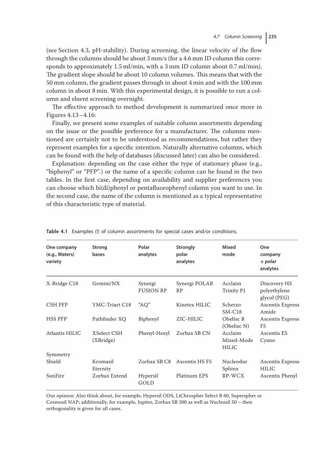
4.7 Column Screening 235

(see Section 4.3, pH-stability). During screening, the linear velocity of the flowthrough the columns should be about 3 mm/s (for a 4.6 mm ID column this corre-sponds to approximately 1.5 ml/min, with a 3 mm ID column about 0.7 ml/min).The gradient slope should be about 10 column volumes. This means that with the50 mm column, the gradient passes through in about 4 min and with the 100 mmcolumn in about 8 min. With this experimental design, it is possible to run a col-umn and eluent screening overnight.

The effective approach to method development is summarized once more inFigures 4.13–4.16:

Finally, we present some examples of suitable column assortments dependingon the issue or the possible preference for a manufacturer. The columns men-tioned are certainly not to be understood as recommendations, but rather theyrepresent examples for a specific intention. Naturally alternative columns, whichcan be found with the help of databases (discussed later) can also be considered.

Explanation: depending on the case either the type of stationary phase (e.g.,“biphenyl” or “PFP”.) or the name of a specific column can be found in the twotables. In the first case, depending on availability and supplier preferences youcan choose which bi(di)phenyl or pentafluorophenyl column you want to use. Inthe second case, the name of the column is mentioned as a typical representativeof this characteristic type of material.

Table 4.1 Examples (!) of column assortments for special cases and/or conditions.

One company(e.g., Waters)variety

Strongbases

Polaranalytes

Stronglypolaranalytes

Mixedmode

Onecompany+polaranalytes

X-Bridge C18 Gemini/NX SynergiFUSION RP

Synergi POLARRP

AcclaimTrinity P1

Discovery HSpolyethyleneglycol (PEG)

CSH PFP YMC-Triart C18 “AQ” Kinetex HILIC ScherzoSM-C18

Ascentis ExpressAmide

HSS PFP Pathfinder XQ Biphenyl ZIC-HILIC Obelisc R(Obelisc N)

Ascentis ExpressF5

Atlantis HILIC XSelect CSH(XBridge)

Phenyl-Hexyl Zorbax SB CN AcclaimMixed-ModeHILIC

Ascentis ESCyano

SymmetryShield Kromasil

EternityZorbax SB C8 Ascentis HS F5 Nucleodur

SphinxAscentis ExpressHILIC

SunFire Zorbax Extend HypersilGOLD

Platinum EPS RP-WCX Ascentis Phenyl

Our opinion: Also think about, for example, Hypersil ODS, LiChrospher Select B 60, Superspher orCosmosil NAP; additionally, for example, Jupiter, Zorbax SB 300 as well as Nucleosil 50 – thenorthogonality is given for all cases.

236 4 Comparison and Selection of Modern HPLC Columns

Comments on Table 4.1

Column 1: Suppose you want to use columns from Waters, because Waters isyour main column supplier. In this fictitious example, you have a completelyunknown sample and for the overnight run using the column switch youwould like to test quite different columns, so you need a variety of Waterscolumns.

Column 2: Suppose you suspect strong bases in your sample and you wouldlike to test columns that are stable under alkaline conditions.

Columns 3 and 4 are self-explanatory.Column 5: These columns are suitable for the case where you expect substances

of completely differing character in your sample.Column 6: The Situation: You want to use columns from Sigma Aldrich and

you know you probably have polar analytes, so you need the entire range ofpolar phases from Sigma Aldrich.

After finding the “best” column overnight, in accordance with our commentsanother run would make sense: better to be safe than sorry, and an orthogonal testin the case of unknown samples provides parallel to a DAD-LC/MS–MS couplingmore security regarding peak homogeneity.

Table 4.2 Examples (!) of column assortments for special cases and/or conditions.

Shapea)

selectivitynew andothers

Shapea)

selectivity… oldSäulen

LowpH-value

2D-separation

Mixedmode ingeneral

Orthogonalityofcolumntypes

ACE 3 C18 Novapak Zorbax SBC18

RP-HILIC RP-WAX C18 Nr. 1:(Atlantis d)

PFP im HILICModus

Nucleosil 50 XSelect CSH RP-SEC RP-WCX C18 Nr. 2:(InterSustain)

ASCENTSExpress Amide

SphersisorbODS 1

YMC Triart IEC-SEC RP-HILIC PEG (Polyethyleneglycol)

Biphenyl Jupiter Gemini/NX Achiral–Chiral HILIC–WAX PFPCosmosilCholesterol

Zorbax SB300

Hypercarb PFP-RP/PFP-NP

HILIC–WCX Biphenyl

Ultra II Aromax Symmetry300

Lichrospher Mixed-ModeRP-NP(SiO2!)

Zorbax ODS Primesep C

a) In such cases, remember the “3”: low flow, methanol as organic solvent, low temperature.Superficially porous material Cortecs, Accucore, PoroShell, Kinetex EVO, Coresep.

Comments on Table 4.2

Columns 1–3 are self-explanatory

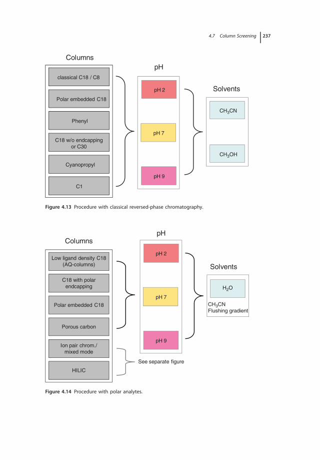
4.7 Column Screening 237

classical C18 / C8

Cyanopropyl

C1

Polar embedded C18

Phenyl

C18 w/o endcapping

or C30

Columns

pH

SolventspH 2

pH 7

pH 9

CH3CN

CH3OH

Figure 4.13 Procedure with classical reversed-phase chromatography.

Low ligand density C18

(AQ-columns)

Ion pair chrom./

mixed mode

HILIC

C18 with polar

endcapping

Polar embedded C18

Porous carbon

ColumnspH

pH 2

pH 7

pH 9

H2O

CH3CN

Flushing gradient

Solvents

See separate figure

Figure 4.14 Procedure with polar analytes.

238 4 Comparison and Selection of Modern HPLC Columns

Weak

cation exchanger,

that is, silica

Weak

anion exchanger

z.B. aminopropyl

but also amide

Neutral

stationary phases,

that is, zwitterionic

(ZIC-HILIC)

or Diol

Columns

pH

Solvents

pH 2

pH 7

pH 9

CH3CN/H2O

Gradient

95 – 70%

CH3CN in

20 Vc

Figure 4.15 Procedure with HILIC.

Bases

Acids

Analytes pH

Solvents

pH 3

pH 7

3<pH<7

5<pH<9

Mixed mode column C18 and

strong anion

exchanger

C18 AQ and Ion pair

reagent,

that is, TBAHSO4

Mixed mode column C18

and weak anion

exchanger

C18 AQ and Ion pair

reagent, that is,

heptane sulfonic acid

Mixed mode column C18

and strong cation

exchanger

Mixed mode column C18

and weak cation

exchanger

pH 3

pH 7

Columns

CH3CN/H2O

Gradient

0 – 100%

CH3CN in

10 Vc

Figure 4.16 Procedure with ion-pair chromatography or by the use of mixed-modecolumns.

4.8 Column Databases 239

Column 4: With 2D experiments (see also Chapter 3) orthogonal selectivitiesare essential. For the given column types, the selection of a suitable mobilephase should not cause any major problems.

Column 5: In addition to examples of modern types of columns with vari-ous combinations of functionality, we have also added Zorbax ODS. As, forexample, LiChrospher, this old classic represents a stationary phase, whichallows almost “all” types of interactions that may be important for a goodselectivity, ranging from hydrophobic interactions (about 17% C) throughion exchange, hydrogen bonding, dipole interactions, and so on to complexformation. The material has among others free, geminal and vicinal silanolgroups, siloxane bonds, and as contaminants metal ions.

Finally, column 6 contains examples of materials that have quite differentcharacters; we have also deliberately included two completely different C18columns.

To the commentary: The more similar the molecules are chemically (also simi-lar polarity) the more important is the use of methanol and chromatographyat low temperatures. Furthermore, higher flows are not allowed due to theslow kinetics.

Recently, several column manufacturers offer selectivity kits for certain pur-poses, for example, Waters offers a family of differently selective columns calledXSelect CSH which is aimed for use with LC/MS compatible mobile phases suchas formic acid.

4.8Column Databases

Often you have a good column, but for some reason it is not available or its pro-duction has been stopped or new production batches of the columns show a com-pletely different selectivity and the separation suddenly no longer works. You mayalso have to prove the correctness of the first method using a preferably orthog-onal HPLC method, or co-elution occurs in a method development. We have allexperienced this during the laboratory routine. The question here is: How do Ifind the most similar or most dissimilar column to my current one?

As so often nowadays, the answer is in the Internet. Under http://apps.usp.org/app/USPNF/columnsDB.html two column databases can be found. Thedatabases contain data from hundreds of HPLC columns, characterized by meansof chromatographic tests such as those described in Section 4.5 [24–27]. The firstdatabase is based on the USP test from the National Institute of Standards andTechnology (NIST) for the characterization of reversed phases. Unfortunately,this test is not very precise.

The second database, the PQRI database, contains data for about 750 columns.The data for each column were determined by means of five chromatographictests carried out at different pH values, so that with this database a very goodcomparison of stationary phase selectivity, also as a function of the mobile phase

240 4 Comparison and Selection of Modern HPLC Columns

Figure 4.17 Screenshot of the PQRI-database.

pH, is possible. The different column parameters are weighted according to thepH of the mobile phase and whether acidic or basic analytes are present in thesample. When, for example, the sample contains no basic analytes, then it wouldbe unnecessary to consider the ion exchange capacity of the two columns whencalculating the fitting factor.

When two columns are compared a fitting factor is obtained, which is a directmeasure of how well the columns match. For any method, the most similar andalso the most dissimilar column to the chosen column can easily be identified, ascan be seen in the figure 4.17. For the sake of completeness, a further database,based on the work of Tanaka, Euerby, and Peterson, is mentioned (ACD Labs Col-umn Selection Database):

http://www.acdlabs.com/products/adh/chrom/chromproc/index.php#colsel.These databases are a great help in finding your way through the jungle of HPLC

columns.

References

1. Iler, R.K. (1979) The Chemistry of Silica,John Wiley & Sons, Inc., New York.

2. Kirkland, J.J. (1972) J. Chromatogr. Sci.,10 (3), 129–137.

3. Horvàth, C. and Lipsky, S.R. (1969) J.Chromatogr. Sci., 7, 109–116.

4. Unger, K.K., Tanaka, N., and Machtjevas,E. (2011) Monolithic Silicas in Separa-tion Science, Wiley-VCH, Weinheim.

5. Dietrich, P.G., Falkenhagen, J., andBertram, R. (2006) Verfahren zur Her-stellung von Aluminiumoxid dotiertem

References 241

Kieselgel zur chromatographischen Tren-nung freier Basen. Deutsches Patent,DE4342493B4.

6. Kromidas, S. (Hsg) (2006) HPLC RichtigOptimiert, Wiley-VCH, Weinheim.

7. Neue, U.D. (1997) HPLC columns, Wiley-VCH, New York.

8. Kromidas, S. (2002) Eigenschaften vonkommerziellen HPLC-RP-Säulen imVergleich, Pirrot Verlag, Saarbrücken.

9. Engelhardt, H. and Jungheim, M. (1990)Chromatographia, 29, 59–68.

10. Engelhardt, H., Arangio, M., andLobert, T. (1997) LC/GC Int., 10 (12),803–812.

11. Kimata, K., Iwaguchi, K., Onishi, S.,Jinno, K., Eksteen, R. et al. (1989) J.Chromatogr. Sci., 27, 721–728.

12. Sander, L.C. and Wise, S.A. (1984) Anal.Chem., 56, 504–510.

13. Sander, L.C. and Wise, S.A. (1987) Anal.Chem., 59, 2309–2313.

14. Sander, L.C. and Wise, S.A. (1995) Anal.Chem., 67, 3284–3292.

15. Neue, U.D. (2007) J Sep Sci, 30, 164ff.16. Stevenson, P.G., Mayfield, K.J., Solivena,

A., Dennisa, G.R., Gritti, F. et al. (2010)J. Chromatogr. A, 1217, 5358–5364.

17. Nyiredy, S., Szucs, Z., and Szepesy, L.(2007) J. Chromatogr. A, 1157, 122–130.

18. Nyiredy, S., Szucs, Z., and Szepesy, L.(2009) Chromatographia, 69, 609–614.

19. Socherl, G., Nussbaum, R., Rissler,K., and Lankmayr, E. (2001) Chro-matographia, 54, 65–70.

20. Tanaka, K., Ding, M.Y., Helaleh, M.I.H.,Taoda, H., Takahashi, H. et al. (2002) J.Chromatogr. A, 956, 209–214.

21. Alpert, A.J. (1990) J. Chromatogr., 499,177–196.

22. Melnikov, S.M., Höltzel, A.,Seidel-Morgenstern, A., and Tallarek, U.(2012) Angew. Chem., 124, 6355–6358.

23. Kriz, J., Adamcov, E., Knox, J.H., andHora, J. (1995) J. Chromatogr., 663,151ff.

24. Snyder, L.R., Dolan, J.W., and Carr, P.W.(2004) J. Chromatogr. A, 1060, 77–116.

25. Snyder, L.R., Dolan, J.W., and Carr, P.W.(2007) Anal. Chem., 79, 3255–3261.

26. Snyder, L.R., Maule, A., Heebsch, A.,Cuellar, R., Paulson, S. et al. (2004) J.Chromatogr. A, 1057, 49–57.

27. Dolan, J.W., Maule, A., Wrisley, L.,Chan, C.C., Angod, M. et al. (2004) J.Chromatogr. A, 1057, 59–74.

243

5Introduction to BiochromatographyJürgen Maier-Rosenkranz

5.1Introduction

During the recent years, biochromatography has increasingly gained in impor-tance, particularly in the pharmaceutical industry for the development, analysis,and production of active pharmaceutical ingredients, the so-called APIs, with asignificantly increased number of biomolecules.

Together with this increased interest in biochromatography, its application anddefinition have also expanded. From a historical perspective, biochromatographydeveloped largely independent from the traditional HPLC, mostly used for smallermolecules (<1000 Da). In most cases, the equipment, columns and packing mate-rials used were provided by other manufacturers. Traditionally, biochromatogra-phy was mostly carried out on polymer-based materials with larger particles inthe low- or medium-pressure range. The use of highly concentrated salt solutionsas mobile phases also made it difficult to apply these methods for classic HPLCsystems. Today, both areas have approached and benefit from each other, thoughthere is still great potential for development in the comprehensive networking ofthese two areas.

Conceptually, biochromatography can be seen as the separation (analysis andpurification) of biomolecules.

Basically, the term biomolecule is broader than usual in chromatographic appli-cations nowadays:

Biomolecules are molecules of organic substances that exist in life-forms. Theymainly consist of carbon and hydrogen, which form chemical compounds withoxygen, nitrogen, phosphorus, or sulfur. Other elements can be a component ofbiomolecules too, though they appear less often. (Source: Wikipedia December 31,2009)

According to this definition, biomolecules comprise a very wide-ranging groupof compounds, which also includes substances such as lipids, phospholipids,glycolipids, sterols, vitamins, hormones, or neurotransmitters. Referring to

The HPLC Expert: Possibilities and Limitations of Modern High Performance Liquid Chromatography,First Edition. Edited by Stavros Kromidas.© 2016 Wiley-VCH Verlag GmbH & Co. KGaA. Published 2016 by Wiley-VCH Verlag GmbH & Co. KGaA.

244 5 Introduction to Biochromatography

Table 5.1 Biomolecules - monomeres.

αα-aminoacid Nucleotide Monosaccharide

O

OH

R

H HN

HO

O

P O

O

OHOH

NN

O–

NN

H2N

HOHO

OH

OHOH

O

biochromatography, this grouping is, however, often reduced to the separationand purification of peptides and proteins.

In chromatographic reality, it is, however, more comprehensive and suitable toextend the definition of biomolecules to include these three groups of substancesand their oligomers and polymers (Table 5.1).

At first sight, sugars play a minor part in this context; they are, however, veryimportant in the glycosylation of peptides or proteins, for example, the glycopep-tide vancomycin.

Table 5.2 lists the 20 proteinogenic amino acids.

Table 5.2 List of the 20 proteinogenic amino acids.

Amino acid Three-letter One-letter Side-chain polarity Groups pI value

Alanine Ala A Nonpolar 6.0Arginine Arg R Basic polar NHR 3× 10.8Asparagine Asn N Polar NH2 –CO 5.4Aspartic acid Asp D Acidic polar COOH 2.8Cysteine Cys C Polar SH 5.1Glutamic acid Glu E Acidic polar COOH 3.2Glutamine Gln Q Polar NH2 –CO 5.7Glycine Gly G Nonpolar 6.0Histidine His H Basic polar Imidazole 7.6Isoleucine Ile I Aliphatic 6.0Leucine Leu L Aliphatic 6,0Lysine Lys K Basic polar NH2 9.7Methionine Met M Nonpolar SCH3 5.7Phenylalanine Phe F Aromatic C6H6 5.5Proline Pro P Nonpolar 6.5Serine Ser S Polar OH 5.7Threonine Thr T Polar OH 5.9Tryptophan Trp W Aromatic Aminoindole 5.9Tyrosine Tyr Y Aromatic OH–C6H6 5.7Valine Val V Nonpolar 6.0

5.2 Overview of the Stationary Phases 245

Primary structure

Secondary structure (left: β-pleated sheet, right: α helix),

Tertiary structure

Quaternary structure

Figure 5.1 Levels of protein structure Source: Wikipedia 2012.

In addition to these primary differences, there are also bigger structural differ-ences as the molecules get bigger.

Table 5.2 and Figure 5.1 show the differences between the various amino acids,peptides and proteins, which can be used for chromatographic separation:

Separation according to Method

Shape/size Size-exclusion chromatography (SEC)Loading Ion-exchange chromatography (IEC)Polarity, solubility Reversed phase; HIC, HILICBiological activity Affinity chromatography (AC)

These six different chromatographic techniques will be explained in detail in thelater sections.

Beforehand, however, the stationary phases will be explained, because the basematerial and its structure and parameters are identical for all chromatographictechniques. The focus is here biochromatographic application and detailed infor-mation to RP materials are in Chapter 4.

5.2Overview of the Stationary Phases

Today, there are a variety of different stationary phases on the market, and it isoften difficult to purposefully select an appropriate phase.

246 5 Introduction to Biochromatography

This section describes the criteria for the evaluation of stationary phases andtheir respective influence on separation efficiency and loading.

5.2.1Base Materials

First of all, the stationary phases differ by the base material used. Ideally, a basematerial is chemically stable against acids, bases and solvents, has good mechan-ical stability (pressure resistance), no change in volume when the mobile phasechanges and no competing interactions with regard to the chromatographicalprinciple used. Unfortunately, not all of these requirements can be realized withthe respective materials. Table 5.3 lists the most common base materials andtheir corresponding classifications.

In addition to these four main materials, there are some others which are, how-ever, not very common: hydroxylapatite, zirconium dioxide, titanium dioxide.

5.2.2Characterization of Stationary Phases

A stationary phase is comprehensively described with the following parameters:particle form and size, pore size, surface area, bonding density, purity andfunctional group. In this context, it is strongly recommended to study themanufacturers information (technical data sheet) and evaluate it according to theseparation to be realized.

Table 5.3 Overview different base materials for Stationary phases.

Silica gels PS/DVBpolystyrenes

Acrylates Dextrans

Mechanicalstability

Pressureresistance

++ + 0 −

Mechanicalstability

Swelling/shrinking

++ 0 − −

Chemicalstability

Solvent ++ + 0 −

Chemicalstability

pHstability – acid

++/≥ 1 ++/≥ 1 +/≥ 2 +/≥ 4

Chemicalstability

pH stabil-ity – alkaline

−/≤ 8 ++/≤ 14 ++/≤ 13 ++/≤ 13

Purity ++ + + +metals (Fe,Al, etc.)

Syntheticby-products

Syntheticby-products

Syntheticby-products

++, applies completely; +, applies partly; 0, applies in a limited way; −, applies poorly.

5.2 Overview of the Stationary Phases 247

5.2.2.1 Particle FormThere are three different particle forms: irregular, spherical and spheroidal. Irreg-ular particles are produced by milling larger particles. This is done with somesilica gels. Previously, this was the primary manufacturing method and, therefore,these silica gels are regarded as out-of-date. Today, however, good irregularsilica gels can be produced, which show very good parameters and, therefore,can clearly be packed better and more stably than the corresponding oldmaterials.

Today, spherical materials are the technical state of the art. Mostly, they can bepacked easily and give a good performance.

Spheroidal forms are less common.

5.2.2.2 Particle SizeThe particle size, dp, is the mean particle diameter and is normally indicated inmicro meter. The particle size defines two important values:

Plate number N ≈ 1∕2 * L/dpPressure P ∼ 1/dp2

If the number of plates is increased by using smaller particles then, as a conse-quence, the pressure increases by square at the same rate.

In this context, the particle size distribution is especially important. Anincreased share of small particles, especially, increases the back pressure. Whenthere are more bigger particles, the number of plates decreases. An additionalproblem of a broad particle size distribution is that the material is more difficultto pack.

If pressure-sensitive soft gels are used and the amount of small particles, so-called fines, is too high, this of course directly influences the field of application(flow rate, column length). In the case of analytical separations, this often doesnot matter much, because pre-packed columns are mostly used. In the case ofpreparative purifications, however, a column with a low number of plates and anincreased back pressure negatively influences the loading, purity, run time, andlifetime.

To evaluate the particle size distribution, besides d50 (=median particle diam-eter) the values for d90 and d10 are normally also indicated.

In Figure 5.2, d50 = 11.2 μm; d90 = 14.4 μm, d10 = 8.7 μm.This means that 90% of the volumes of all particles are smaller than 14.4 μm

and that 10% of the volumes of all particles are smaller than 8.7 μm. For an eas-ier evaluation and better comparability, mostly d90/d10 are defined. The value ford90/d10 should be as small as possible: suitable values are less than 2. The examplein Figure 5.2 shows a d90/d10 = 1.66, which is good.

The advantage of the smaller particles to show a better resolution because ofthe higher plate number is used directly for better analyses. Today, materials from

248 5 Introduction to Biochromatography

0

10

1.3

2.5

3.7

4.9

6.1

7.3

8.5

9.6

10.8

12.0

13.2

14.4

15.6

16.8

18.0

19.2

20.4

21.6

20

30

40

50

60

70

80

90

100%

vo

lum

e

Particle size distribution

Particle size distribution

Figure 5.2 Particle size distribution meassured by laser diffraction.

1.5 to 5 μm are typical, or up to 10 μm in the case of materials with low pressurestability. In the case of preparative separations and high loadings, the advantageof smaller particles is less important, as can be seen in Figure 5.3.

When smaller particles are used, the peak broadening caused by loading isclearly higher than with bigger ones. The selection of the particle size depends,of course, on the given separation and is normally a compromise betweenresolution, loadability, and the possible pressure and flow rate ranges. In the

00

20

40

60

80

100

Pe

ak w

idth

at

ha

lf h

eig

ht

(mm

)

120

140

160

200 400 600

10 μm

5 μm

20–30 μm

15–20 μm

800 1000

Ribonuclease load (μg)

Figure 5.3 Protein loading capacity of RP-HPLC materials of different particle sizes. Source:Protein and Peptide Analysis and Purification, Vydac Reversed Phase Handbook, 5th edition,W.R. Grace, 2013.

5.2 Overview of the Stationary Phases 249

preparative scale, 5 μm is only used if highest performance is needed, such asfor the purification of synthesized peptide obtained from a synthesizer withimpurities having only small differences to the target peptide. The consequenceis that the loading is limited.

5.2.2.3 Pore Size and SurfaceBiomolecules exist in a very broad size range. Therefore, it is very important toselect the right pore size. Traditionally, the pore size is indicated in angstrom,10 Å= 1 nm. Phases with smaller pores have a bigger surface and thus more pos-sibilities for interaction. They can also have a higher loading:

60 Å ∼500 m2/g120 Å ∼300 m2/g200 Å ∼200 m2/g300 Å ∼120 m2/g1000 Å ∼30 m2/g

Depending on the molecule weight the following pore sizes are suitable:

60 Å <1 000 MW120 Å <10 000 MW200 Å <50 000 MW300 Å <100 000 MW500 Å <250 000 MW1 000 Å >250 000 MW

These values are only approximate, because the pore availability depends on thesample molecules topology and the pores themselves. The indication of the porediameter always refers to the unbonded base material. Depending on the bonding,the available space in the pore is reduced.

It is important for chromatography to have a very tight pore size distribution toguarantee that the given surface is also available chromatographically. In the caseof a broad pore size distribution, most of the surface is in the small pores, which arenot available to bigger molecules. It is, therefore, possible that stationary phaseswith nominally bigger pores and thus a smaller surface nonetheless have morecapacity, because the surface in the bigger pores is better available due to betteraccessibility.

The pore size and distribution are defined by nitrogen adsorption (BET) or mer-cury porosimetry. In chromatographic terms, inverse size-exclusion chromatog-raphy (SEC) is particularly suitable, because only those pores are measured thatare chromatographically available.

250 5 Introduction to Biochromatography

0.0

w(ϕ

)

1.0 2.0 3.0

Log ϕ(nm)

Figure 5.4 Inverse size-exclusion chromatography from two different polystyrene phases.Source: J. Maier-Rosenkranz, PhD thesis, Tübingen, 1992.

In Figure 5.4, two polystyrene phases are compared. W shows the respectiveshare of the different pore diameters (Φ) in the total pore volume. One aspecttypical of polymer materials is the high proportion of microporosity and a poresize distribution, which tends to be broad. In this example, the pore size distribu-tion is particularly broad; especially for the phase indicated with -•- a very highmicroporosity can be detected, and the proportion of bigger pores is evenly dis-tributed over all sizes. Therefore, for bigger molecules only a very limited share ofthe surface is available. For RPC or IEC, a phase of this type would be unsuitable;for SEC, however, it would cover a broad molecular range with a good selectiv-ity. The second phase, indicated with -•-, shows much less microporosity and ahigh proportion of pores with log Φ from 0.8 to 1.8, which corresponds to a porediameter of 60–600 Å.

Figure 5.5a,b depicts the separation of paracelsin, a peptide (20-mer) with foursequence analogs, which differ only slightly, on an RP silica and a PS/DVB phase.The separation on the silica-based phase can be realized in about a quarter of thetime used for the separation on the PS/DVB phase. In this case, this big differencecan largely be attributed to the tighter pore size distribution of the silica-basedphase.

5.2.2.4 Loading Density

The loading density is an important information for the selection of the stationaryphase. Depending on the functional group, it is indicated differently.

In the case of reverse phases, it is indicated as %C or in μmol/m2, and inthe case of ion exchangers in μeq/ml or μeq/g. In addition to this, there is thedynamic binding capacity, which indicates the capacity for a determined proteinfor a given flow rate. The dynamic binding capacity depends, of course, on thetype and size of the sample molecules, the flow rate and the pore accessibility.

5.2 Overview of the Stationary Phases 251

(a)

(b)

Figure 5.5 (a) Separation of paracelsin on a silica-based C8 phase. (b) Separation ofparacelsin on a PS/DVB phase. Source: J. Maier-Rosenkranz, PhD thesis, Tübingen, 1992.

From a chromatographic point of view, it is the more important value, becauseit best reflects the real conditions. A high loading does not automatically meana high capacity. If big molecules are adsorbed at the surface, accessibility to theneighboring groups is reduced, which means that these groups are not available.There are, therefore, also low-loaded stationary phases, because these can offeradvantages over high-loaded ones.

5.2.2.5 PurityBecause biomolecules are multifunctional, they can of course interact witheach other. Impurities in the base material can unintentionally interact with thesample, which can worsen the chromatography and even lead to a completeadsorption.

Normally, purity is specified as a percentage and should be greater than 99%.Metals such as Al and Fe, which mainly exist in silica gels, should not exceed

10 ppm, or the surface coverage is so good that it is not important any more fromthe chromatographic point of view.

252 5 Introduction to Biochromatography

The main impurities are mostly by-products of polymerization. These can beboth monomers or shorter polymer units and starters or emulsifiers.

5.2.2.6 Functional GroupThe functional groups are described in the respective chapters on the chromato-graphic techniques.

5.3Reversed-Phase Chromatography of Peptides and Proteins

RP chromatography is one of the standard methods for analyzing peptides andproteins. It stands out for a very good selectivity and performance.

One of the most common methods is the use of trifluoroacetic acid (TFA) inwater against acetonitrile gradients. TFA has the advantages that it reduces the pHvalue, the carboxyl groups are protonized, and it forms an ion pair with the aminogroups. Thus, the peptide or protein has no more free charges and, therefore, it isas hydrophobic as possible.

If none of the information that is important for chromatography is available,the starting point is normally a screening gradient of 5–95% 0.1% TFA againstACN 0.1% TFA. The following sections describe the different parameters for thedevelopment and adaptation of methods.

5.3.1Retention Behavior of Peptides and Proteins

The retention of a small molecule is reduced when the ACN content increases.Roughly estimated: +10%B∼ 1/2 tR

The retention of a protein is suddenly reduced as soon as the critical pointbetween adsorption and desorption is reached. This means that even changes of±1%B decide if the protein has retention or if it passes through with t0. Figure 5.6shows the various graphs from k to %B. The bigger the peptide or protein thesteeper these curves are, which means that it is more difficult to realize stable andreproducible retention times under isocratic conditions. Therefore, the gradientelution is preferred for peptides and proteins.

5.3.2Gradient Design

As already described, the chromatography is normally started with a screeninggradient between 5 and 95% 0.1% TFA to ACN 0.1% TFA. As a rule of thumbfor the gradient duration, it takes 1 min/cm column length and, in the case ofmore complex samples, 2 min per column length. In a second step, the gradientis adapted such that the peaks are spread over the total time range. Usually, verygood selectivities are achieved with this approach.

5.3 Reversed-Phase Chromatography of Peptides and Proteins 253

0.0

10.0

20.0

30.0

40.0

50.0

60.0

70.0

0 20 40 60 80

k-va

lue

%B

Small molecule

Protein

Figure 5.6 Influence of change %B on k.

The following gradient parameters influence separation selectivity:

Gradient slope: %/mindefined by the difference between the start and final concentrations as wellas the time (gradient duration)

Gradient volume: mldefined by flow rate and time

Reducing the gradient slope by increasing the gradient time is normally thefastest and easiest way to improve the resolution (Figure 5.7).

The second way to influence the resolution is to change the gradient volume.Traditionally, there are two ways to scale when changing to another column. Inthe case of linear upscaling/downscaling, the gradient duration is scaled at thesame rate as the change in the column length:

column length halved = gradient times halved

In this case, the gradient volume is halved. The second way is to keep the gradientvolume constant: time is adapted at the same rate as the column length changesand, at the same time, the flow rate is changed such that the same quantity ofeluent is always flowing through the column:

column length halved = gradient times halved + flow rate doubled

Today, the constant gradient volume is mostly applied when changing from thetraditional HPLC to UHPLC. If a column of 15 cm is changed to that of 5 cm, thegradient duration is reduced to 1/3 and the flow rate is tripled.

Both ways can lead to success. The result for method development is that, witha given column length and gradient duration, the variation of the flow rate is criti-cally important. Because, as described in Section 5.3.1, different substances show

254 5 Introduction to Biochromatography

0.25% /min

0.5% /min

Figure 5.7 Influence of the gradient slope onresolution. Vydac 218TP C18, 4.6× 150 mm,10 μm; 25–50% ACN in 0.1% TFA ml/min.Sample: Subunits of cytochrome c oxidase.

Source: Protein and Peptide Analysis andPurification, Vydac Reversed Phase Handbook,5th edition, W.R. Grace, 2013.

different behaviors when the organic modifier (%B) is increased, the k-values alsoshow different behaviors when the flow rate is increase or reduced. This can alsolead to a change in the peak sequence. Therefore, varying the flow rate by ±50%as a minimum is recommended. It must, however, be taken into considerationthat, depending on the pore size, access to the pores is more difficult with highflow rates and big molecules and that, therefore, the Van Deemter curve stronglyincreases.

5.3.3Organic Modifier

Acetonitrile is undoubtedly the most used organic modifier for analytic andpreparative (laboratory scale) separations. The reasons for this are its goodefficiency, low viscosity and low UV adsorption at wavelengths of approximately210 nm.

Alcohols such as methanol, ethanol, and isopropyl alcohol are not as popularbecause of their high viscosity and the high back pressure resulting from it. Yet,these protic solvents strongly influence selectivity, especially of polar peptides orproteins on polar RP phases (C8, C4, CN, phenyl, diol). For the method develop-ment, it is, therefore, recommended to use and to vary mixtures of acetonitrile andalcohol as organic modifiers. This is often more efficient and faster than changingthe stationary phase.

Ethanol and isopropyl alcohol are often used at a process scale, because theseare cost-effective, and they can more easily be applied in the regulatory environ-ment. It is also easier to keep up biological activity in comparison to acetonitrile,

5.3 Reversed-Phase Chromatography of Peptides and Proteins 255

which has a stronger denaturing effect. The use of isopropyl alcohol is, further-more, favorable when hydrophobic peptides or proteins are separated, which canalso increase recovery.

5.3.4Ion Pair Reagent

TFA is the most common ion-pair reagent. The low pKs value (0.8) protonizesthe carboxyl groups and, therefore, retention is higher than with formic acid oracetic acid, with pKs values of 3.75 or 4.76. The typical concentration is 0.1%. Anincrease in the ion-pair concentration results in the peptides and proteins tend-ing to have a higher retention. Because this increase is different for the respectivepeptides or proteins, concentration is an important parameter for the methoddevelopment.

With basic peptides and proteins, in particular, heptafluorobutyric acid (HFBA)can be used alternatively for TFA, which has the advantage of more sharper peaks.Another advantage of these two ion-pair reagents is their high UV transmittanceat short wavelengths. With LC–MS applications TFA and HFBA are less oftenapplied, because both cause a strong ion suppression. Good results are, however,achieved by combining ion-pair reagents with acids. To achieve sufficient capacity,formic acid is used in higher concentrations together with very low concentrationsof HFBA or TFA to get the low pK s value (see Figure 5.8).

Theoretically, other acids, such as phosphoric acid or hydrochloric acid, can alsobe used, because these can also positively influence selectivity. The reason for theirrare use is, in the case of hydrochloric acid, its high potential for corrosion, andphosphates are not volatile, which is an exclusion criterion in the case of MS orpreparative applications.

In the neutral pH range, ammonium formiate, ammonium acetate, and triethy-lamine phosphate and in the alkaline range ammonia, trimethylamine, and tri-ethylamine are used.

Columns that are to be used with ion-pair reagents should be reserved for thisapplication only. Otherwise, there is a very high risk of a change in selectivity andassociated with this, bad reproducibility.

5.3.5Influence of the pH Value

Amino acids, as components of peptides and proteins, are zwitterions, that is,they have both positive (–NHR2

+) and negative charges (–COO−) depending onthe solutions pH value. If the amino acid has the same number of positive andnegative charges, namely at the pI value, it is neutral. Below the pI value, the pep-tides are cations and above it they are anions. The pI value of acidic amino acids isapproximately 3, that of the polar, non-polar, and aromatic amino acids is 5–6.5and that of the basic ones is greater than 7 (see Table 5.1).

256 5 Introduction to Biochromatography

0

Inte

nsity (

×1

08)

0.0

0.2

0.4

0.6

0.8

1.0

1.2

1.4 2 60.2% FA

1. Oxytocin, 1007 Da (Cys-Tyr-lle-Gln-Asn-Cys-Pro-Leu-Gly-NH2)

2. Bradykinin, 1060 Da (Arg-Pro-Pro-Gly-Phe-Ser-Pro-Phe-Arg)

3. Angiotensin II, 1046 Da (Asp-Arg-Val-Tyr-lle-His-Pro-Phe)

4. Neurotensin, 1672 Da (pGlu-Leu-Tyr-Glu-Asn-Lys-Pro-Arg-Arg-Pro-Tyr-lle-Leu)

5. Angiotensin I, 1296 Da (Asp-Arg-Val-Tyr-lle-His-pro-Phe-His-Leu)

6. Eledoisin, 1188 Da (pGlu-Pro-Ser-Lys-Asp-Ala-Phe-lle-Gly-Leu-Met-NH2)

0.2% FA, 0.01% HFBA 0.2% FA, 0.01% TFA

3

5

1 4

4

4

6

6

5

5

3

32

21 1

2 4 6 8 10 12 14 16 18 20

Time (min)

0 2 4 6 8 10 12 14 16 18 20 0 2 4 6 8 10 12 14 16 18 20

Figure 5.8 Effect of the combination ofion-pair reagents. LC–MS TIC of peptides.Column: Vydac® Everest® 238 EV, 300 Å,C18, 5 μm 150× 1 mm. Mobile phase: A:95:5% water: ACN with ion-pair reagents. B:20:80% water:ACN with ion pair reagents.

Flow: 50 μl/min, gradient: 12.5–50% Bin 30 min. Source: Protein and PeptideAnalysis and Purification, Vydac ReversedPhase Handbook, 5th edition, W.R. Grace,2013.

Depending on the peptide or protein structure, the number and distri-bution of the charges, and thus the molecules polarity, change with the pHvalue. This obviously has a direct influence on retention and selectivity (seeFigure 5.9).

In the acid pH range, acid peptides have less charge and thus a higher retention;this is true for basic peptides in the basic range. During method development, thepH value is one of the dominant factors and if, in the acid pH range, the stan-dard method with TFA or HFBA has no success, it is a good way to regulate thenecessary selectivity via the pH value.

5.3.6Pore Size

Section 5.2.2.3 already described the pore size influence in combination with sta-tionary phases. Therefore, only the particularly RP-relevant points are specifiedhere. Normally, stationary phases between 100 and 300 Å are used for peptides.The bigger pores, in particular, have the advantage of better accessibility. This isnot only an advantage during chromatography, but also during the bonding. Due

5.4 IEC Chromatography of Peptides and Proteins 257

1. Bradykinin2

3

1

5

1+2

3

4

53

2

5

1+4

(a) pH 2.0 (b) pH 4.4 (c) pH 6.5

4

2. Oxytocin3. Angiotensin II4. Neurotensin5. Angiotensin I

Figure 5.9 Separation of a peptide mix-ture at different pH values. Column Vydac®218TP, 300 Å, C18, 4.6× 250 mm, 5 μm.Mobile phase/gradient: 15–30% ACN in20 mM phosphate, (a) pH 2.0, (b) pH 4.4,(c) pH 6.5. (1 ml/min). Sample: 1. bradykinin,

2. oxytocin, 3. angiotensin II, 4. neurotensin,5. angiotensin I. Source: Protein and PeptideAnalysis and Purification, Vydac ReversedPhase Handbook, 5th edition, W.R. Grace,2013.

to the fact that alkyl silanes get better into the pores, materials with bigger poresoften have a better surface covering and thus fewer unwanted interactions withthe base material. In the analytic separation, this can, for example, be seen fromthe fact that the peak form is better or that low-concentration impurities can beseen and not adsorbed completely on the surface.

5.3.7Bonding Chemistry

Usually, C18, C8, C4, phenyl and CN phases, or even polystyrenes are used forthe RPC of peptides. The bonding used depends on the polarity, size, and higherstructure of the peptides or proteins. Polar phases (C8, C4, phenyl, CN) tend tobe used for polar compounds, because they have a higher selectivity in the polarrange. C18 is usually used for lipophilic compounds, because it has the best solu-bility thanks to its high amount of ACN that is needed for elution. If the lipophilicpeptide or protein sticks to the surface, polar phases are used too. In this case, itmust be ensured that, when the amount of water increases, the peptide or proteinis still soluble. In the case of bigger peptides or proteins, shorter chains (C4) areadvantageous, because then the accessibility to the pores is increased.

5.4IEC Chromatography of Peptides and Proteins

There are two types of ion-exchange chromatography (IEC): cation chromatogra-phy, that is, the separation of cations, which is used for proteins/peptides at a pH

258 5 Introduction to Biochromatography

value below their isoelectric point, and anion chromatography, that is, the separa-tion of anions, which is used for proteins/peptides at a pH value higher than theirisoelectric point or for oligonucleotides or polynucleotides.

The respective stationary phases are as follows:

Strong cation exchanger (SCX)S (methylsulfonate) –CH2SO3

−

Sulfopropyl (SP) –CH2CH2CH2SO3−

Weak cation exchanger (WCX)Carboxymethyl (CM) –OCH2COO−

Strong anion exchanger (SAX)Quaternary ammonia (Q) –NR3

+

Weak anion exchanger (WAX)Diethylaminoethyl (DEAE) –CH2CH2N+(CH2CH3)2Diethylaminopropyl (ANX) –CH2CHOHCHH2N+H(CH2CH3)2Quaternary aminoethyl (QAE) –OCH2CH2N+(C2H5)2CH2CH(OH)CH3

In this relation, “strong” or “weak” does not mean the interaction strength, butthe change in capacity of the ion exchanger depending on the pH value. Strongexchangers are available over a wide range with a constant capacity. As regardsweak exchangers, the capacity changes in correlation with the pH value.

With IEC, the column is loaded at a low salt concentration and when the saltconcentration increases, it elutes (see Figure 5.10).

20

1 3

25

4

40 60 min

Column phase: GROM-SIL 300 WCX, 7 μm

Column size: 250 mm × 4.6 mm

Eluent A: 0.05 M NaH2PO

4, pH 6.4

B: 0.5 M NaH2PO

4, pH 6.4

Gradient: 0–18%B (0–21 min), 18%B (21–26 min),

18–60%B (26–70 min)

Flow rate: 1.0 ml/min

Pressure: 7 MPa

Temperature: RT

Detection (UV): 280 nm

Injection: 100 μl

(1) Trysinogen

(2) Ribonuclease A

(3) Cytochrome C

(4) Chymotrypsinogen

(5) Lysozyme

Figure 5.10 Example of ion-exchange chromatography. Source: Grom Analytik+HPLCGmbH, Application 09105; 2004.

5.4 IEC Chromatography of Peptides and Proteins 259

5.4.1IEC Parameters

5.4.1.1 Ionic Strength of the SampleProteins and peptides with a higher ionic strength have a higher retention. Theionic strength is, above all, defined by the number of charges.

5.4.1.2 Buffer Concentration of the EluentAn increase in the buffer concentration results in shorter retention times. Usually,gradient separation is preferred. Resolution is usually set via the gradient slope.Flatter gradients increase resolution. In Figure 5.10, for example, an isocratic stepis used to separate the cytochrome from the chymotrypsinogen.

5.4.1.3 pH ValueThe pH value influences not only the samples charge conditions, which influencethe selectivity strongly, but also those of the exchanger. At very low pH values, theacid group of cation exchangers is protonized and is thus not available for chro-matography. If the pH value is higher, the retention of SCX and WCX increases,because more loadings are available on the ion exchanger.

The behavior of the anion exchanger is exactly the opposite. If the pH values arehigher, SAX and WAX have a shorter retention.

Instead of a salt concentration gradient, a pH gradient can also be used. In thiscase, eluting conditions are if the pH value moves toward the samples pI value –there is no more retention at the pI value – or, as explained above, the charge num-ber on the exchanger is reduced.

This variant can be applied for LC–MS, because this avoids large quantities ofsalt, which would significantly reduce the sensitivity of the analytic of peptidesand proteins.

5.4.1.4 Organic ModifierTo improve solubility or to suppress unwanted interactions, it is possible to addan organic solvent, similar to RP chromatography. If ACN or alcohols are added,retention is reduced. For ESI-LC–MS, particularly, this is an advantage, becausethe mobile phase can be sprayed more easily with the organic solvent, whichallows the salt concentration to be kept low. It can also be a good idea to use agradient. The use of a gradient supports elution and selectivity.

5.4.1.5 TemperatureAn increase in temperature usually improves kinetics, which causes the peaks tobe narrower. The temperature also influences the pH value and the samples inter-actions. This also changes selectivity.

260 5 Introduction to Biochromatography

5.4.1.6 Flow Rate

Normally, the flow rate is slightly smaller than with RP-HPLC: 0.5–0.8 ml/minfor a column of 4.6 mm. This corresponds to a linear flow rate between 4.3 and6.9 cm/min. A good indication for a suitable flow rate is the dynamic capacity,which is usually specified in the technical data sheet. In the case of very bigmolecules, a low flow rate can be advantageous.

5.4.1.7 Pore Size

As already described in Section 5.2.2.3, the pore size selected defines the availablesurface.

5.4.1.8 Loading and Injection Volume

Because of the strong interactions, IEC can focus big injection volumes at thecolumn head very well. It is also possible to highly load ion exchangers. Loadingdepends on many parameters (all the parameters described above), but it is partic-ularly dependent on the size of the sample molecules and the static and dynamiccapacity.

IEC is a suitable complement or alternative to RP chromatography. The elu-tion and selectivity can be adjusted in very different ways. Figure 5.11 shows a

Column phase: GROM-SIL 120 Amino-3 CP, 5 μm

Column size: 250 mm × 4.6 mm

Eluent A: 5 mM KH2PO

4, pH 2.9, 15% ACN

B: 500 mM KH2PO

4, pH 4.0, 15% ACN

Gradient: 40–100%B (0–20 min), 100%B (20–25 min)

Flow rate: 2 ml/min

Pressure: 14 MPa

Temperature: RT

Detection (UV): 254 nm

Injection: 10 μl (160 μg/ml)

(1) GMP

(2) AMP

(3) IMP

(4) GDP

(5) ADP

(6) IDP

10 20 min

1

2

3

4

56

Figure 5.11 IEC of nucleotides using salt-, pH- and organic solvent-gradient Source: GromAnalytik+HPLC GmbH, Application 07127; 2004.

5.5 Size-Exclusion Chromatography of Peptides and Proteins 261

combination of salt concentration gradient, pH gradient and the addition of anorganic modifier.

First, the monophosphates elute, then the diphosphates follow much later,because of the double charge.

IEC can even be used in LC–MS if the traditional salt gradient is replaced orreduced by changing the pH value and the concentration of the organic modifier.This broadens the field of application even further.

5.5Size-Exclusion Chromatography of Peptides and Proteins

SEC is a special form of chromatography, which differs in the fact that there are(ideally) no interactions with the stationary phase.

The principle of separation is based on the different pore accessibilities of dif-ferent molecule sizes. Small molecules can penetrate all pores and therefore, havea longer way, very big molecules are completely excluded and thus elute first (seeFigure 5.12).

Separation is, therefore, based on the different available volumes. In the follow-ing, the volume types for a column of 300× 8 mm are specified.

Column volume 15 ml 100%Interstitial volume: V i ∼4 ml ∼30%Pore volume: V P ∼7 ml ∼45%Volume of the mobile phase (dead volume): V 0 ∼11 ml ∼75%Volume of the stationary phase ∼4 ml ∼25%

Volume available for separation V 0 −V i =V P ∼7 ml

Injection Mobile phase

Stationary phase

with mobile phase

in the pores

Sample 1 – small molecule

Sample 2 – large moleculeSeparation

Detection/

collection

Figure 5.12 Principle of size-exclusion chromatography.

262 5 Introduction to Biochromatography

At a flow rate of 0.5 ml/min, the time up to the first peak (completely excluded)would be at approximately 8 min and for the last peak (completely penetrating, t0)at approximately 22 min.

In the case of SEC, the chromatogram finishes – at t0 – at the point when sep-aration starts with other chromatography techniques.

At first sight, the mobile phase thus does not influence separation either,because, theoretically, there are no interactions. In reality, however, unintendedinteractions take place, which must be prevented with the mobile phase.

Ionic interactions With a high salt concentration, pH valueRP interactions With an organic modifierSolubility With an organic modifier, pH value

In Figure 5.13, a typical SEC separation can be seen. The phosphate bufferadjusts the pH value, the sodium chloride produces the high salt concentration,and the ACN acts as an organic modifier.

With this type of separation, the possible selectivity can also be assessed. Pep-tides or proteins, whose molecular weight differs by approximately a factor of 2,

10 20

Column phase: GROM-SIL 200 SEC, 5 μm

1

2 3

4 5

30 40 50 min

Column size: 500 mm × 8 mmEluent: 0.1 M K-phosphate, 0.2 M NaCl, pH 7.0 / ACN = 70 / 30Flow rate: 0.7 ml/minPressure: 5.2 MPaTemperature: 26 °CDetection (UV): 280 nm, 0.08 AUFSInjection: 15 μl (~10 mg/ml, each)

(1) Glutamate dehydrogenase

(MW 290 000)

(2) Lactate dehydrogenase (MW

142 000)

(3) Enolase (MW 67 000)

(4) Adenylate kinase (MW 32 000)

(5) Cytochrome C (MW 12 000)

Figure 5.13 SEC separation. Source: Grom Analytik+HPLC GmbH, Application 09046b; 2004.

5.5 Size-Exclusion Chromatography of Peptides and Proteins 263

Dextran blau 2 000 000 D

β-Galactosidase 50 0000 D

BSA dimer 13 0000 D

Amyloglukosidase 97000 D

γ-Globulin 90 000 D

BSA monomer 67 000 D

Carboanhydrase 30 000 D

Myoglobin 18 000 D

Cytochrom 13 000 D

Insulin 6000 D

Tyrosin 180 D

Dextranblau 2 000 000 D

β-Galactosidase 50 0000 D

BSA dimer 130000 D

Amyloglukosidase 97 000 D

γ a-Globulin 90 000 D

BSA monomer 67 000D

Carboanhydrase 30 000 D

Myoglobin 18 000 D

Insulin 6000 D

Tyrosin 180 D

Cytochrom 13 000 D

100 1000 10000 100000

MW

1000000

4.6 mm ID Säule

0.3 mm ID Säule

min

10000000

Stationäre Phase: TOSOH Super SW 2000 - 4 μm Säulendimension: 300 mm × 4.6 mmbzw. 0.3; Eluent: 0.,1 M Na-Phosphat pH 6.8 - 0, 1M NaCI; Fließgeschwindigkeit:0.35 mm/s; Temperatur: RT; Detektor: 206 nm (UV); Flusszelle: 15 μl / 10 mm bzw. 4 nl/ 0.2 mm; Injektion: 10 μl bzw. 300 nl Proteinlösung (~ 0.1–0.5 mg/mL)

Figure 5.14 SEC curve. Source: Application Note No 005, Grom Analytik+HPLC GmbH,2003.

can easily be separated. The retention time/molecular weight graph shows therange in which different molecular weight gives the change of the elution time. InFigure 5.14, this range goes from 6000 D (insulin) to 500 000 D (𝛽-galactosidase).The field of application for the stationary phase depends on the pore size.

5.5.1SEC Parameters

SECs performance is influenced by the following parameters:

5.5.1.1 Particle Size

The particles should be as small as possible to get short diffusion paths and narrowpeaks. The disadvantage of small particles is the increased back pressure, whichcan cause problems depending on base materials such as acrylate or polystyrene.

5.5.1.2 Pore Size Distribution

A narrow pore size distribution causes a good separation for a small MW rangeof peptides and proteins. Broad pore size distribution allows separations over a

264 5 Introduction to Biochromatography

broad MW range with lower selectivity. This is usually balanced out with longercolumns.

5.5.1.3 Pore VolumeThe pore volume defines the possible run time/elution volume of the separation.The higher it is, the higher the peak capacity is and the chance of a good separation.

5.5.1.4 Flow RateLower flow rates are showing higher plate numbers. Low flow rates allow partic-ularly bigger molecules to diffuse better into the pores. In the case of high flowrates, these are, as a tendency, shifted toward lower elution volumes.

5.5.1.5 TemperatureA higher temperature reduces viscosity and, therefore, allows a better diffusion.Efficiency increases. Proteins, however, are temperature sensitive and, therefore,the temperature increase is limited.

5.5.1.6 ViscosityA lower viscosity increases efficiency. Viscosity can be influenced by the type ofsalt, the salt concentration, and the organic modifier.

5.5.1.7 Loading and Injection VolumeBoth of these should be as low as possible. As SEC has no retention, both param-eters directly affect the peak broadening.

5.6Further Types of Chromatography – Brief Descriptions

In addition to the types of chromatography described earlier in detail, three othertypes can be used for biochromatography.

5.6.1Hydrophobic Interaction Chromatography

With hydrophobic interaction chromatography (HIC), hydrophobic proteinsinteract with slightly hydrophobic surfaces (propyl, ether, phenyl) at high saltconcentrations. For elution, a salt gradient from high to low salt concentrationsis used (see Figure 5.15).

5.6.2Hydrophilic Interaction Chromatography

Hydrophilic interaction chromatography (HILIC) is particularly used for stronglypolar compounds, that is, if these have a low retention at RP chromatography or

5.6 Further Types of Chromatography – Brief Descriptions 265

(1) Cytochrome C

(2) Myoglobin

(3) β-Lactoglobulin

(4) Ribonuclease A

(5) Lysozyme

(6) α-Chymotrypsin

(7) Chymotrypsinogen

10 20 30 min

1

2

34

5

6

7

Column phase: GROM-SIL 300 HIC, 7 μm

Column size: 250 mm × 4.6 mm

Eluent A: 2.0 M (NH4)2SO

4 – 0.1 M KH

2PO

4, pH 6.8

B: 0.1 M KH2PO

4, pH 6.8

Gradient: 0–100% B (0–30 min)

Flow rate: 1.0 ml/min

Pressure: 8 MPa

Temperature: RT

Detection (UV): 280 nm

Injection: 100 μl

Figure 5.15 Example of an HIC protein separation. Source: Grom Analytik+HPLC GmbH,Application 09106; 2004.

if the peptides to be separated mainly differ in the polar groups. It is often appliedfor separating different degrees of glycosylation of a peptide.

The HILIC functional principle can be described as follows. On polar phases,polar molecules have retention when solvents that are more nonpolar than the sta-tionary phase and that can be mixed with water are used. A layer of water developson the phases surface. The polar sample spreads between this layer of water andthe mobile phase.

Amino, diol, cyano, SAX, SCX, Si, and a series of special polar groups are usedas stationary phases. Acetonitrile/water is usually used as a mobile phase, butmethanol, ethanol, isopropyl alcohol, or a mixture of them are also common. If theamount of acetonitrile is increased, retention increases. If water is added, reten-tion is reduced. The addition of acids, bases, and buffers is possible and is used formethod development (Figure 5.16).

5.6.3Affinity Chromatography (AC)

With affinity chromatography (AC), the biospecific interactions between, forexample, a protein and the matching antibody are used to separate the proteinor the antibody. This separation is based on a specific and reversible interactionbetween the molecules. A typical application is the purification of monoclonalantibodies. Under the given conditions, they bond to a stationary phase that iscovered with the protein A. After a washing step, the conditions are changed(often change in the pH value) such that the antibody elutes.

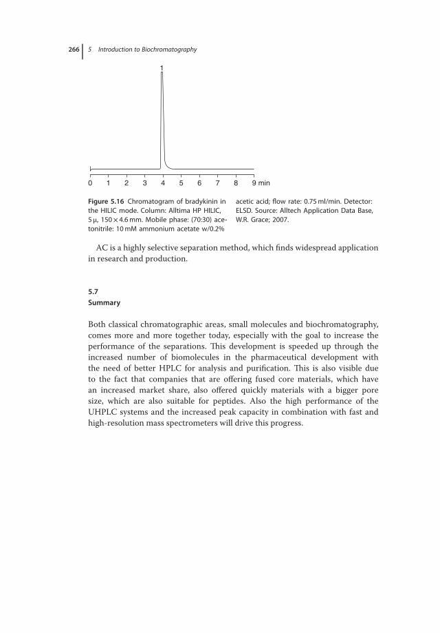
266 5 Introduction to Biochromatography

0 1 2 3 4 5 6

1

7 8 9 min

Figure 5.16 Chromatogram of bradykinin inthe HILIC mode. Column: Alltima HP HILIC,5 μ, 150× 4.6 mm. Mobile phase: (70:30) ace-tonitrile: 10 mM ammonium acetate w/0.2%

acetic acid; flow rate: 0.75 ml/min. Detector:ELSD. Source: Alltech Application Data Base,W.R. Grace; 2007.

AC is a highly selective separation method, which finds widespread applicationin research and production.

5.7Summary

Both classical chromatographic areas, small molecules and biochromatography,comes more and more together today, especially with the goal to increase theperformance of the separations. This development is speeded up through theincreased number of biomolecules in the pharmaceutical development withthe need of better HPLC for analysis and purification. This is also visible dueto the fact that companies that are offering fused core materials, which havean increased market share, also offered quickly materials with a bigger poresize, which are also suitable for peptides. Also the high performance of theUHPLC systems and the increased peak capacity in combination with fast andhigh-resolution mass spectrometers will drive this progress.

267

6Comparison of Modern Chromatographic Data SystemsArno Simon

6.1Introduction

The field of modern chromatography data systems (hereinafter CDS) now extendsfrom the single-user solution for separate measuring systems to global networksolutions in which laboratories from different countries and across continentswork together. Hardly any other area in the analytical laboratory has changed sosignificantly as the laboratory data processing. The developments and the differ-ences between these systems are presented here as well as the attempt is made togive an outlook on the next developments and trends.

The range of application for modern CDS runs today from single workplacesof separated analytical systems to global network solutions, where laboratories ofdifferent countries and continents collaborate in the same infrastructure. It canbe assumed that no other area in the analytical laboratory has changed to such asignificant extent as the management of laboratory data. This chapter presents thedevelopment and differences of these systems and tries to give a look-out to thenext development steps and trends for the future.

6.2The Forerunners for CDS

The triumphal procession of CDS started 30 years ago with the enhancementsof the integrator. Based on contemporary computer platforms, such as digitalVAX, a DEC professional or an HP1000, several manufacturers for HPLC andGC instruments have developed integration software programs for the controlof their instruments and the evaluation of their chromatograms. All of themhad a restricted scope of operation, compared with current standards, and wereextremely cost-intensive. First, the IBM PC and the following clone-PCs wereaffordable for a conventional laboratory and have, therefore, been the cause formore and more manufacturer to invest into this sector of industry. With the

The HPLC Expert: Possibilities and Limitations of Modern High Performance Liquid Chromatography,First Edition. Edited by Stavros Kromidas.© 2016 Wiley-VCH Verlag GmbH & Co. KGaA. Published 2016 by Wiley-VCH Verlag GmbH & Co. KGaA.

268 6 Comparison of Modern Chromatographic Data Systems

IBM PC entering the laboratories, the environment for the operational computersystem has changed from UNIX-based central computers to MS-DOS and lateron Windows-based office clients.

Over the years, the scope for software systems as a kind of an alternative integra-tor for the evaluation of peaks and quantification with limited tuning options haschanged to complex solutions that were able to control many different instrumentsand to manage laboratory samples.

6.3CDS Today

The first and perhaps most important difference of current CDS is how data stor-age is organized. Until 1992, when Waters has introduced the Millennium2010 soft-ware, all established solutions were based on file-based data storage, as it wasknown for MS office programs. But Waters Millennium2010 has used an integrateddatabase for storing analytical data. While file-based systems save all informa-tion such as sample name in the data name of the data file and the instrumentmethod including all settings in a method file, Millennium2010 stores these datain a database. By this solution, new possibilities for the management of analyticaldata were given. Especially, method information has been saved again and againtogether with each new data file in order to provide traceability. With a databasesolution, all information and results are stored associated in a database having alink to the corresponding injections.

A database solution offers the possibility to easily search for any informationdemanded by the user. For example, the changes of retention times for a definedcompound that should be considered over a longer period can be depicted inMillennium (a later on in Empower) by simple database query, where each firstinjection of a standard solution over the past 6 months is considered.

More and more manufacturers are following this idea and equip their CDS moreor less halfhearted with a database. In many cases, only the administration of rawdata files has been moved to a database, whereas the actual meta data (sampleinformation, measuring data and results) are still stored as files.

Currently, all modern CDS have an integrated database. But file-based systemsdo still have advantages today.

6.4Advantages and Disadvantages of File-Based CDS

File-based CDS store all information in single data files. This way, in most cases, amethod file, which contains measuring and evaluation settings, and sequence file,defining the sample order of a measuring set, are stored together with the actualraw data files. These files are structured by a typical folder structure on the acqui-sition computer or on a network drive. For most users, this system gives the best

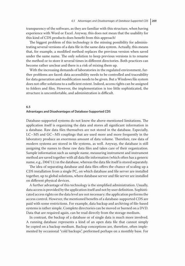
6.5 Advantages and Disadvantages of Database-Supported CDS 269

transparency of the software, as they are familiar with this structure, when havingexperience with Word or Excel. Anyway, this does not mean that the usability forthis kind of CDS products does benefit from this approach!

The biggest problem of this technology is the missing possibility for adminis-trating several versions of a data file in the same data system. Actually, this meansthat, for example, a modified method replaces the previous version when savedunder the same name. The only solution to keep previous versions is to renamethe method or to store it several times in different directories. Both practices canbecome rather unclear and there is a risk of mixing them up.

With the increasing demands of laboratories in the regulated environment, fur-ther problems are faced: data accessibility needs to be controlled and traceabilityfor data generation and modification needs to be given. But a Windows file systemdoes not offer solutions to a sufficient extent. Indeed, access rights can be assignedto folders and files. However, the implementation is too little sophisticated, thestructure is uncomfortable, and administration is difficult.

6.5Advantages and Disadvantages of Database-Supported CDS

Database-supported systems do not know the above-mentioned limitations. Theapplication itself is organizing the data and stores all significant information ina database. Raw data files themselves are not stored in the database. Especially,LC–MS and GC–MS couplings that are used more and more frequently in thelaboratory produce an enormous amount of data volume. Therefore, raw data ofmodern systems are stored in file systems, as well. Anyway, the database is stillassigning the names to these raw data files and takes care of their organization.Sample information such as sample name, measuring instrument and instrumentmethod are saved together with all data file information (which often has a genericname, e.g., D04711) in the database, whereas the data file itself is stored separately.

The idea of separating database and data files offers the chance of scaling up aCDS installation from a single PC, on which database and file server are installedtogether, up to global solutions, where database server and file server are installedon different physical devices.

A further advantage of this technology is the simplified administration. Usually,data access is provided by the application itself and not by user definition. Sophisti-cated access rights on the data level are not necessary; the application performs theaccess control. However, the mentioned benefits of a database-supported CDS arepaid with some restrictions. For example, data backup and archiving of file-basedsystems is rather simple. Complete directories can be moved or burned on a DVD.Data that are required again, can be read directly from the storage medium.

In contrast, the backup of a database or of single data is much more involved.A running database represents a kind of an open data file that cannot simplybe copied on a backup medium. Backup conceptions are, therefore, often imple-mented by occasional “cold backups”, performed perhaps on a monthly base. For

270 6 Comparison of Modern Chromatographic Data Systems

those cold backups, the database needs to be stopped. In addition, daily “hot back-ups” are performed, where all modifications since the last backup are stored. In thecase of a roll-back, first the latest “cold-backup” needs to be retrieved followed byall “hot-backups” generated after this. This can take a while.

Especially, for installations of a manageable size, the virtualization offers newchances.

On a virtualized host, the hardware of a CDS server is emulated. This virtualizedCDS server runs as application on that host, what offers several advantages:

• Servers use the computing capacity only to a little extent. As the hardware of avirtualized host is used by several virtual servers, the hardware capacity can beutilized more efficiently.

• With increasing performance requirements for a CDS server, for example, byan increasing number of registered users, more storage or processor capacitycan be assigned to the virtual machine without the need of adjusting the CDSinstallation.

• The possibility to retain the current status of the CDS server by a so-called“snapshot” permits to save the systems before the installation of patches andupdates, what could be very comfortable for test systems.

• The backup of a running database server is more difficult due to the high numberof open data. Therefore, the database needs to be stopped, before a backup canbe performed. Operation of the CDS is suspended during this time. As a virtualserver actually depicts a single data file, data backup programs are available onthe market that can even save running databases. The operation of the CDS doesnot need to be suspended.

6.6CDS in a Network Environment

More and more companies are integrating their CDS in the companies’ ownnetwork environment. Provided that the CDS supports network capability, manyadvantages are offered:

• Access to system and data is given from any PC in the network.• Users can, for example, prepare and start their analyses in the laboratory,

whereas the evaluation can take place in the quiet office room.• Data are stored at a central location, which simplifies data backup.

A file-based network environment mostly consists of single workstations, whichuse a common storage for data files in the network. The whole software function-ality is granted to every workplace.

In contrast, a database supported system has the database server as a centralnode in the network. Here, data acquisition clients are connected to for controllinganalytical instruments and acquiring data, which then will transfer the data tothe server. The user works at a client PC, where the evaluation part of the CDSsoftware is installed.

6.7 Instrument Control 271

On a data acquisition client, there is no other software installed except the CDS.As the user will never work actively on such a client and, for example, using theinternet, there is no risk caused by malware or incompatibilities. The separation ofinstrument control and data acquisition on the one hand and the workplace clientson the other hand is an important factor for the stability of such systems. This wayit is guaranteed that instrument control and data acquisition work reliably and nomeasuring data become lost, even if a problem occurs in the network or on theserver.

Where the CDS is used for monitoring and operating production processes, theavailability of the system is of high importance. Network interruptions or down-times of a database server can potentially tie up the complete fabrication. The elab-oration of an emergency concept is, therefore, of enormous significance. Althoughresearch laboratories can easily come to terms with an outage of, for example,1 day, even a few hours downtime can be a big problem for in-process control lab-oratories. Therefore, conceptions that correspond to the individual requirementsneed to be established and tested. Often these concepts are not easy to develop,as the availability of a database server of a database-supported CDS is an essentialprecondition.

ThermoSCIENTIFIC (Dionex) is a CDS manufacturer that has presented aninteresting solution on this with Chromeleon 7. The system copies the part of thecentral database that is relevant for an analytical instrument on the data acquisi-tion client. In the case where the connection to the database gets lost, work can becontinued with this local copy of the database. Once the database connection hasbeen reestablished, the contents of the local copy and the central database will besynchronized.

6.7Instrument Control

Originally, all CDS were control and evaluation systems of one instrument man-ufacturer. The aim was to provide a better and more convenient control of thein-house HPLC and GC instruments. As the solutions were always focused onthe own instrument hardware, almost every manufacturer uses his own systemto connect instruments to the computer hardware. Besides standardized formatssuch as IEEE488 Bus (Waters & Agilent), there can be found serial interfaces, lateron often USB ports or proprietary connections. In correlation with standardizedcommunication protocols, this can lead to incompatibilities, why some laborato-ries have decided to use several CDS each having its particular data system. Inorder to decrease the effort that arises from training laboratory staff and multipleinstallations, maintenances, and software validations, companies aim to decreasethe number of CDS in their laboratories to a minimum. Having the focus on oneCDS helps to define a unique workflow and ensures a consistent documentationof the processes.

272 6 Comparison of Modern Chromatographic Data Systems

For reaching this aim without being forced to replace a multiplicity of analyticalinstruments, the number of different instruments that can be controlled by a CDShas become a decisive aspect. No CDS manufacturer can get away with only beingable to control his own instruments.

When surveying the currently available CDS products with regard to their capa-bility of controlling different instruments, the following can be observed:

• Manufacturers, where the instruments have a big market share, have startedlately to integrate external instruments. For them, the present instrumentswhere the key to place their software in the laboratories.

• Manufacturer with a small market share must be able to control various instru-ments in order to get a chance of placing their software. Formerly, the con-trol of the competitors’ instruments has been realized by reading the data buswithout the permission of the manufacturer. Today, the control codes are oftenexchanged between single suppliers.

• Manufacturers that do not have own chromatography instruments give licensesfor their CDS to manufacturer of instruments without an own software; theCDS integration can be programmed by themselves. This kind of integration isin most cases very successful.

6.8Documentation and Compliance

With the entrance of the information technology, the US Food and Drug Admin-istration (FDA) has increased the demands for documentation. Especially, GxPareas in pharmaceutical industries, but also suppliers of the chemical industriesare concerned. Information that formerly simply was filed in paper format is todaya matter of strong obligations regarding traceability and secure data storage. Thisresults in two basic requirements:

• All data and the ways of their generation need to be traceable.• Electronic data must sometimes be archived for long periods during which their

readability must be ensured.

A high degree of traceability has already been reached by optimized controloptions for chromatography instruments.

Besides the chromatogram, the instrument method is stored as well. In addition,the single work steps of the user, from the start of a measurement to the final result,must be stored in a traceable manner. In this aspect, database-supported CDSoffer high benefits. Relations between single information can simply be depictedin a database, whereas file-based systems are charged with a redundant amountof information.

However, regarding the demand of archiving data, file-based systems offer oneof the few advantages: As all data are kept in simple folder structures, those can

6.9 Brief Overview of Current Systems 273

easily be transferred to corresponding longtime storage media and placed intostock.

From a database, where all information is linked to each other, single data cannotbe removed readily and stored somewhere outside the database. For archiving,there is either a corresponding structure required or the CDS already offers specialfunctionalities that make archiving possible.

6.9Brief Overview of Current Systems

It seems to be impossible to provide an entire overview of all CDS that are cur-rently on the market. Every now and then, some trade magazines are publishingoverviews where the different functionalities are compared. But these compar-isons do not really offer an objective view. Almost all systems have an audit trailfunction today, but the functional scope differs a lot between the single systems.Knowing that it is impossible to offer a real objective comparison, the most com-mon systems should be presented from a subjective point of view. Besides someinformation about the CDS itself, the mentioned advantages and disadvantagesreflect the ratings and perceptions of different users. Anyway, everybody is free tomake his own appraisal.

6.9.1Atlas

For many years, the standard CDS of ThermoSCIENTIFIC has been Atlas.With the acquisition of Dionex, the more modern and more powerful soft-ware, Chromeleon has become a product of ThermoSCIENTIFIC. Therefore,the decision was taken to replace Atlas by Chromeleon during the next years.Before this, the control of additional ThermoSCIENTIFIC instruments and thesupport of MS need to be implemented in Chromeleon. With Chromeleon 7.2that was announced for the middle of 2013, this implementation should becompleted.

6.9.2ChemStation

Agilent ChemStation is a well-proven and a popular software product. Over theyears, the software has achieved a high degree of distribution, particularly at uni-versities and public institutions. The software design of ChemStation has becomeout-of-date over the years. That’s why Agilent has started a redesign, calling thesoftware now OpenLAB.

Strengths: reasonably priced, easy to use.Weaknesses: low performance, file-based software architecture.

274 6 Comparison of Modern Chromatographic Data Systems

6.9.3Agilent OpenLAB CDS

In 2010, Agilent started launching Agilent OpenLAB CDS. Agilent talks about anevolution of its software instead of calling it a new CDS. Two versions are cur-rently available on the market: the ChemStation and the EZchrom edition. Bothof them use the same control panel module and the same report generator. Allother software parts are adjusted to the customs of ChemStation and EZchrom,respectively.

This approach is less spectacular than the introduction of a new product. Any-way, a soft and less extensive changeover is possible.

Strengths: modern network technology, large integration into the OpenLABfamily, for example, direct search in OpenLAB ECM from the CDS.

6.9.4Chromeleon

Particularly, in Europe, Chromeleon could take root as a significant and great CDS.With version 7.0 introduced in 2010 and 7.1 released in the beginning of 2011, afully new product has been developed. Strengths of the previous version 6.8 havebeen kept, and weaknesses have been eliminated forcefully.

Strengths: easy to use, support of the most common HPLC and GC instruments,database-supported architecture.

Weaknesses: MS support is not supported yet (planned with the introductionof version 7.2).

6.9.5Empower

With Empower and its parent product Millennium2010, Waters is the pioneer fordatabase-supported CDS. With the current version Empower3, the final stage ofadvancements is supposed to be reached. Currently, Waters is developing a suc-cessor called UNIFI that follows a new conception and a redevelopment from thescratch: the combination of CDS, Electronic Lab Notebook (ELN), and ScientificData Management System (SDMS).

Weaknesses: not easy to learn, support of controllable instruments could beextended. Software has reached the final stage of its life cycle.

6.9.6EZchrom

Agilent has obtained the EZchrom software with the acquisition of Scientic Soft-ware. Over the years, EZchrom has become the core part of many other CDS. Justas ChemStation, the EZchrom software has been revised and is called OpenLABCDS EZchrom Edition.

6.9 Brief Overview of Current Systems 275

Strengths: a multiplicity of instruments can be controlled.Weaknesses: low performance, file-based architecture.

6.9.7Tabular Comparison of Empower and Chromeleon

Both ThermoSCIENTIFIC Chromeleon and Waters Empower cover the wholerange of requirements of a modern CDS. Both are network capable (up to 1000users and more) and can be run in a terminal server environment. Anyway,differences can be discovered going into detail, even though those are regardedand judged from a subjective point of view. In the following table, the existingdifferences are compared:

Empower 2 Empower 3 Chromeleon

6.8

Chromeleon

7.x

OpenLAB

CDS

Support ofcurrent OS

No (onlyWindows Vistaand Windows2003 Server)

Yes Yes Yes Yes(32 bit and64 bit)

Supporteddatabases

Only Oracle Various (Oracle, SQL,MS-Access)

Oracle andSQL (file-based asalternative)

Integratedoutageprotection

Limited (running dataacquisitions arecontinued, evaluationand starting of newmeasurements is notpossible)

Yes (in case of anoutage the wholerange of operationscan be continued onan acquisition client)

YesOperationson a clientare possibleFailover

Usability Difficult (but easyaccess to functionalitiesof the database)

Easy adapted to thecommon use ofWindows Explorer.Difficult for databasequeries

Easy

GUI Traditional Windows Design withmenu and toolbar

Current MS Officeribbon design

276 6 Comparison of Modern Chromatographic Data Systems

Empower 2 Empower 3 Chromeleon

6.8

Chromeleon

7.x

OpenLAB

CDS

Support ofMS detectors

Yes (some Waters MSdetector)

No Yes(Version 7.2)

Yes

Support ofcompetitiveinstruments

Yes (limited to HPLCinstruments ofShimadzu, Hitachi,Dionex and AgilentGC & HPLCSystems, andBeckman CE)

Yes (broad range of instruments fromdifferent manufacturers)

Peakintegration

Easy (graphical appliance,with ApexTrack almostautomatic)

Normal (likeall commonsystems)

Easy(graphicalappliance,withSmartpeakIntegrationwellsupported)

Modern(dataanalysis)

Integratedautomatiza-tion

Yes, but limitedInjections as part of aSample Set can berepeated or aborteddriven by the calculatedresult

Yes, butlimitedconditionscan bedefined inmethods –difficultto set

Ja byso-calledeWorkflowsprocessescan bedepicted

Ja SmartSequenz

Reporting Reports can bedesigned individually,complex layouts arepossible. Graphicaleditor is offeredcalculations that areembedded in the reportare only possible to arestricted extent (tablestatistics)

Reports offer almost thesame possibilities as MSExcel, Even complexcalculations are possible

Intelligentreportbuilder.(based onMS BIS)

6.10 The CDS of Tomorrow 277

Empower 2 Empower 3 Chromeleon

6.8

Chromeleon

7.x

OpenLAB

CDS

Customizingby owndatabasefields

Any number ofuser-defined databasefields can be created.Those can containdescribing information(e.g., batch number),but also complexcalculations (betweenpeaks of the samechromatogram andbetween differentsample lines)

Any numberof additionaldatabasefields can becreated.Those cancontaindescribinginformation(e.g., batchnumber),calculationsinuser-defineddatabasefields are notpossible

Any numberof additionaldatabasefields can becreated.Those cancontaindescribinginformation(e.g., batchnumber),calculationsinuser-defineddatabasefields are alsopossible

Yes,alpha-numericinforma-tiononly

Versioningof results

All methodmodifications are storedas a new methodversion, overwriting ofdata is not possible.Each result that wasgenerated and storedcan be retrieved at anytime

Versioning ofmethods isnotsupported.Results arenot stored,but createdagain eachtime fromthe scratch

All methodchanges areautomaticallystored as anew version.Data cannotbeoverwritten

Yesmethodversionsandresultsets

6.10The CDS of Tomorrow

6.10.1MS Integration

In the same way, as 20 years ago the diode-array detector became the defaultdetector in the laboratories, MS detection has become rather popular. Evenquestions and answers concerning data technology were very similar: Unusual

278 6 Comparison of Modern Chromatographic Data Systems

data amounts need to be stored, operated, and backed up. At that time, thediscussion was focused on megabyte ranges, whereas today giga- and terabytesneed to be handled. As long as mass spectrometers are used as stand-alone instal-lation in specific MS laboratories, the workplace is the most practical solution.Inexpensive NAS systems (network attached storage) are easily capable to store adata volume of 10 terabytes that can be transferred over a decided network to anacquisition or evaluation client. In the case where mass spectrometers today areintegrated into a CDS, the infrastructure needs to be adapted to the postulatedrequirements. Unfortunately, strong and suitable solutions are not yet offered byany manufacturer.

6.10.2Large Installation

More and more global companies extend their CDS to an installation across theirlocations over the world. The aim is to harmonize the processes by centralizing thedata, in order to reduce costs and expenses for operating the system. A company-wide installation has many advantages, where different models can be considered:

With licenses organized by the concurrent user model, only active user accountsare counted, which are concurrently working with the CDS. By this model, thesame licenses could first be used by a site in, for example, Japan and later on in theUnited States due to the time shift.

Using licenses according to the named user model, every single active accountin the system is counted, no matter if this user has currently registered in the sys-tems or not. Costs for licenses are saved by keeping unused licenses centrally. Forexample, each single site does not need to keep three “spare-licenses,” but centrallyfive licenses are kept that can be offered to any site, if requested.

Centralization reduces costs for testing, validation, and documentation. Insteadof having the effort for user management, data storage, and validation of user-defined calculations for many sites, this can be taken care of centrally only oncebeing valid for all sites. The single laboratories connected to the system can simplyaccess the already validated system and can refer to a centrally managed documen-tation. It is very obvious how expenses to run such a CDS can be reduced. As alldata are stored at a central location and are not distributed at the single sites of acompany, backup and archiving strategies as well as a conception for an outage ofthe system can be implemented much more easily.

However, company-wide installations still involve a big risk. A huge amount ofdata needs to be organized and managed. Although a database mostly can handlethe high amount of data volume, the storage volume for data files is in most cases aproblem. According to the selected security concept of the software, for example,copying of data into the companies’ storage area network (SAN) could be mis-leadingly interpreted as data manipulation by the CDS. With UNIFI Waters hasannounced a new solution, where data files are kept in the database themselves.Administration of a large installation would be much easier by this approach.

6.11 Special Extensions 279

A central system demands much more planning for administrating and per-forming updates. Especially, global installations only offer a few slots, where nouser is working in the system, for example, performing a reboot of the server. Forthe installation of updates that need to be distributed on all servers and clients atthe same time, several hours of even days are required, where the system is notavailable for the daily operation.

6.10.3Easy and Intuitive Usability

For many years, CDS manufacturers have implemented new functionalities in thesystem that are now offered by a modern CDS and that cover almost all require-ments for the operation in laboratory. Unfortunately, usability has suffered withthe implementation of new functionalities. Most systems require a 5-day trainingcourse, in order to qualify the user for running the most important functions. Forupcoming functional changes and enhancements that are implemented by a soft-ware update in the current CDS installation, new concepts are necessary in thefuture, in order to avoid a complicate operation and missing transparency.

With the release of Chromeleon 7, ThermoSCIENTIFIC has focused on usabil-ity aspects by reducing forcefully the number of required clicks for performinga special task and by offering a modern graphical user interface in the style ofMS Office. MS Office 2007 only displays the menu items that are required for theselected task.

Apple has demonstrated how the user acceptance of a product will increase byan elaborate usability. It will be interesting to see how manufacturer, especiallyWaters, is going to provide for this challenge with its new product UNIFI.

6.11Special Extensions

Already today, different suppliers offer extensions and interfaces to their CDS.Those extensions increase the functional scope of the software or solve specialproblems or requirements. Some of these ideas are demonstrated in the followingsections.

6.11.1Support of Peak Integration

All CDS offer various possibilities for the integration of chromatograms. The aimof an integration is to determine the peak area as precise as possible. For thispurpose, the integration needs to precisely follow the baseline. Where the useris unsure, all systems offer an overlay function by which, for example, the chro-matogram can be compared with a blank injection. The blank depicts the bestbaseline course. Much more difficult to identify the “correct” integration for non-baseline separated peaks. Here, the CDS offer three different integration types:

280 6 Comparison of Modern Chromatographic Data Systems

1) Peaks can be separated by setting a drop line.2) A peak can be skimmed from a mother peak by a tangential line (tangential

skim).3) A peak can be skimmed from a mother peak by an exponential curve (expo-

nential skim).

Especially, the integration performed by a drop line and an integration per-formed by a skimming might provide very different peak area values. For example,when determining impurities and degradation products, the kind of integrationwill decide whether or not a product meets the specifications and still can be used.An assistance for the decision, which integration should be used, no CDS is offer-ing today. Anyway, additional programs are available that can be connected to thesoftware through a programmed interface. These extensions offer a mathematicalwell-founded rating and can support the decision in case of an audit.

6.11.2Column Administration

Some suppliers have integrated the installed analytical column in their hardwaresystems for identification purposes. This can be performed by a “funk chip” that isconnected to the column and can be recognized by the column compartment (Agi-lent) or by a clip that is connected to the column that is then fixed at the columncompartment (Waters).

Here, the compatibility is the biggest problem again: Column information can-not be assigned to the corresponding injection in the CDS. If it would be possibleto store the clear identification of a column for each injection automatically in theCDS, a column log book could be depicted without any additional effort.

6.11.3Instrument Usage

In times of increasing competitive constraints, companies are more often delib-erating whether the investment of a new chromatographic instrument is requiredor if the present instruments could be charged better to capacity. All informationto support such a decision are actually stored in the CDS. Anyway, they cannot beexploited just like that.

The first step would be a summary of all run times of an instrument. But thisonly provides the actual measuring time. Times for equilibration and injectionsthat are not stored in the CDS also need to be considered. All these times providein summary the actual usage time of an instrument.

In addition, it needs to be considered that samples are measured as a series(sequence or sample set) in most cases. In order to judge the real usage, the timesbetween two series needs to be considered, as well. In case of an idle running ofperhaps 1 h no further samples could be measured during this time. If beyond thatthe column needs to be replaced and solvent need to be changed, even periods

6.11 Special Extensions 281

of several hours could not be used for additional measurement. A functionalitythat provides information about the usage of an instrument and the detection ofidle running would be very helpful, but is not part of any current CDS and can,therefore, only be implemented by a third party software program. Such a featureneeds to have access on all data that have ever been generated by a system. For thispurpose it is necessary to store all relevant data in separate database, a so-calleddata warehouse. Using the currently present information in the CDS, all data thatalready have been archived or deleted would be missing and the result of a querywould not reflect the effective usage of an instrument.

6.11.4Connection of Balances

Almost for every measurement that is performed by HPLC or GC systems, sampleweightings need to be performed in advance. No matter if a sample weighting orif a solution for a reference solution is prepared, always measuring values from abalance are involved.

For a laboratory with a paperless workflow, these values are kept in the Lab-oratory Information and Management System (LIMS) and will be transferred tothe CDS. Without this cross-linking, the manual input of weightings into the CDSwould signify an enormous effort and the risk of transcription errors would exist.To avoid this, two approaches for the transfer of balance data to the CDS arethinkable:

First instrument driver of a balance could be connected directly to the CDS andtransfer the values through this interface, for example, into the sample table of aCDS. However, although this seems to be a simple solution, there is a little pitfall:standard solutions are often prepared for the use of a defined period. The measur-ing value of a standard that was prepared on a Monday still needs to be availableon a Tuesday. Does the expiry end after 3 days, this value must not be used on Fri-day. An administration of standard values, therefore, needs to be provided. Wheresolutions are available for later measurements until their expiry date.

If a weighting consists of several steps, the measuring value from the balanceis not the value that should be used in the CDS. For example, 12 mg of substanceA are weighed and 15 mg of substance B are added, the actual balance displays avalue of 27 mg. Before transferring the values to the CDS, a difference betweenweighing A and weighing B needs to be calculated.

For this reason, a direct interface between the balance and the CDS is only pro-ductive for easy processes. The second solution should, therefore, be preferred:

Through an interface the CDS is connected to the balance software. Besides themere data acquisition, current software products such as labX of Mettler-Toledoprovide support for the measurement itself. Operation procedures (first weigh anempty measuring flask, then add about 15 mg of substance A, fill up with water)and further important information such as limits (15 mg of substance A in therange of 13–17 mg) can be transmitted to the user.

282 6 Comparison of Modern Chromatographic Data Systems

Instead of connecting a balance directly to a CDS, the integration of a balancesoftware provides more functionality and a higher comfort.

6.12Open Interfaces

Although CDS have been considered as an independent system so far, now across-linking becomes necessary with the increasing significance of the integra-tion of various software systems. For example, a LIMS delivers the work ordersto the laboratory, which then should be executed by the CDS. The obtaineddata then need to be evaluated somehow and retransferred to the LIMS. Across-linking between LIMS, CDS, ELN, and SDMS is avoiding manual transfererror and provides potential for saving time and securing data that should not bemisprized. Even the time-consuming review of transferred data is inapplicable.Unfortunately, there is today almost no harmonization of interfaces and data for-mats. Only the standards according to AIA, a definition of the American Societyfor Testing and Materials (ASTM), offers a possibility for simple transfers ofCDS data between the different systems. In the future, the current ANDI/netCDFstandard is supposed to enable the exchange of 3D data, as they are generated bydiode array detectors and mass spectrometers.

However, these formats only permit the transfer of mere measuring data (XY-data files) and eventually of some meta data, such as the sample name. Up to now,a real connection, where access is given to all information of the CDS including allmeasuring results, always needs to be customized as an individual solution. Eveninterfaces that are offered by some LIMS and CDS suppliers do not really offeran out-of-the box conception, but rather a tool box that allows the customer tocreate his own solutions. Here, new concepts are desirable that could simplify thecross-linking between different systems.

It is supposed that Waters offers a new approach with the UNIFI system. Thebasic idea is that all systems of a laboratory access the same data pool in thedatabase. Here, the single components CDS, ELN, and SDMS can be connectedto, which are required by the customer. By using a shared database all connec-tion steps are obsolete, and the single system could cooperate seamlessly. The onlyquestion that has not been solved yet is how systems of other suppliers could dockon. In case UNIFI will be kept as a proprietary Waters system, this concept couldnot be considered as a comprehensive approach for the laboratory of tomorrow.

6.12.1Instrument Integration

Today, not all instruments can be connected to every CDS in the laboratory. As aresult, some laboratories need to purchase several CDS. To avoid this, suppliers forinstruments and CDS should offer corresponding interfaces for the developmentof instrument drivers in the future. Up to now, the attempt has failed to harmonize

6.13 The CDS in 20 Years 283

interface for instrument drivers, as in contrast to the supplier-independent inte-gration of printer drivers in Windows, every supplier of analytical instrumentsuses his own protocol.

At least, Agilent has started with an attempt of harmonization offering theInstrument Control Framework (ICF). A CDS supplier only needs to implement adriver for the ICF interface, Agilent cares for the connection of the driver to theinstrument. By this, a better integration of the instrument to the CDS is givenand drivers are available more quickly, as only Agilent needs to develop a newimplementation. An agreement on a general standard for interfaces would alsohelp the user in harmonizing and reducing test and validation procedures. Usertrainings would be simpler as the graphical interfaces for entering control settingswould look similar for all systems.

6.13The CDS in 20 Years

Which trends would find their way into the future of the CDS?Comparing the systems of today with the standards of the 1980s, it can be

assumed that the CDS of the 2030s would also look completely different.One trend, which can already be suspected today, is the migration of the CDS

from a local installation into a cloud. Due to the globalization, there are systemstoday where data are stored separated from their point of origin. For the user,the chromatogram can be found in the CDS – the actual storage location doesnot matter. In a next step, the application itself could be located in the cloud. Thecloud is probably followed by mobile devices. Instead of the conventional PC, theuser of the future will presumably walk with a tablet PC through the laboratory.On standing in front of an HPLC, the instrument would recognize the tablet PCby RFID technique and the CDS could transmit the current measurement, as wellas all other entries such as, for example, audit trail.

Acknowledgment

Finally, I thank my colleague Ingo Green for his remarks and ideas, which were ofgreat help for the preparation of this chapter.

285

7Possibilities of Integration TodayMike Hillebrand

Let us imagine a perfect chromatographic method. Every single component of asample would be displayed as a fine single graph.

But (especially) in biotechnology or in the chemistry of natural products, this isnot usual.

For example, if substances are generated by microorganisms, the by-productsobtained are often very similar to the main product. And this will cause peakswith overlapping areas, which cannot be often separated completely.

7.1Peak Overlay - Effect on the Chromatogram

If two peaks do overlap, this does not mean that one is hiding behind the other.Both signals are combined. So the signal from components A and B, and otherpossible components is assembled. The result is a sum curve or envelope.

Overlapping peaks always run the risk of making errors in area integration. Asthis is a systematic error, it usually remains undetected. Therefore, in the methoddevelopment, baseline separation of the peaks is desirable. The larger the peak sizeratio, the better the resolution needs to be. However, as explained in the introduc-tion, even with enormous strain in method development, in some cases, a baselineseparation is not possible.

If you have overlapping peaks, you have to be aware that you do not onlyhave errors in area integration, but also in retention time and height. Both areaffected by the peak overlay, this is shown in Figure 7.1. Both parameters are veryimportant peak parameters, since they are used for quantitative and qualitativeterms.

Figure 7.1 shows three overlapping peaks. The analyst would receive only thedark grey sum curve in his chromatogram. It consists of the combined signalsof the three peaks (light gray). As you can see, each peak affects its neighbors,because the rise or fall of the respective neighbors, in turn, affects the cumulative

The HPLC Expert: Possibilities and Limitations of Modern High Performance Liquid Chromatography,First Edition. Edited by Stavros Kromidas.© 2016 Wiley-VCH Verlag GmbH & Co. KGaA. Published 2016 by Wiley-VCH Verlag GmbH & Co. KGaA.

286 7 Possibilities of Integration Today

40000

3500

3000

2500

2000

1500

1000

500

0

0 0.5

Sum curve Compound 1 Compound 2 Compound 3

1 1.5 2 2.5 3

−500

Δ Height

Δ Height

Δ tR

Figure 7.1 Effect of peak overlay on the determination of the peak height and retentiontime.

curve. So, the height and the retention time of the peaks, depending on the reso-lution varies can change within the cumulative curve.

7.2Separation Techniques for Higher-Level Peaks

Having overlapping peaks in a chromatogram, the analyst has to solve thefollowing question: “Which separation method is the best for separating theseoverlapping peaks?”

The vertical separation method (“Vertical skim,” “drop”), separation of thetangential (“skim Tangential”), the valley-to-valley separation method, the Gaussseparation method (“Gaussian skim”), or the exponential removal (“Exponentialskim”)?

Looking at the separation methods, you can see very quickly (just consider thevertical, the tangential, and the valley-to-valley separation method) that the sep-aration must be faulty and full of “errors.”

Overlapping peaks and overlaid curves can only be determined in exceptionalcases by separating with straight lines.

7.2.1Lot Method

The vertical peak separation, which is called Lot method, separates peaks fromeach other by drawing a vertical line.

This is preferably (depending on the resolution or size) placed in the valleybetween the peaks (see Figure 7.2a).

7.2 Separation Techniques for Higher-Level Peaks 287

4500

4000

3500

3000

2500

2000

1500

1000

500

−500

00 0.5 1 1.5

Sum curve

Sum curve

2 2.5 3

4500

4000

3500

3000

2500

2000

1500

1000

500

−500

00 0.5 1 1.5

Sum curve

Sum curve

2 2.5 3

4500

4000

3500

3000

2500

2000

1500

1000

500

−500

00 0.5 1 1.5

Sum curve

Sum curve

2 2.5 3

4500

4000

3500

3000

2500

2000

1500

1000

500

−500

00 0.5 1 1.5

Sum curve

Sum curve

2 2.5 3

4500

4000

3500

3000

2500

2000

1500

1000

500

−500

00 0.5 1 1.5

Sum curve

Sum curve

2 2.5 3

4500

4000

3500

3000

2500

2000

1500

1000

500

−500

00 0.5 1 1.5

Sum curve Compound 1 Compound 2 Compound 3

2 2.5 3

Δ Height

Δ Height

Δ tR

Figure 7.2 For available separation tech-niques for higher-level peaks and their com-parison ((a) vertical separation, (b) tangentialseparation, (c) valley-to-valley separation, (d)

Gauss separation method, (e) exponentialseparation, (f ) comparison, cumulative curvewith single peak).

Mistakes/errors that may occur to the “Vertical skim” in terms of area analysisare described by V.R. Meyer and confirmed in several scientific work area rules.

7.2.2Error by the Vertical Skim Overlapping Peaks (Area Rules to V.R. Meyer) [1]

• Symmetric peaks: the large peak is too large and the small is too small (regardlessof elution) [1].

• Peaks with tailing: the first peak too small and the second to great (regardlessof the area ratio) [1].

• The ratio of the relative error is inversely proportional to the ratio of the peakareas [1].

288 7 Possibilities of Integration Today

• Small peaks are more affected [1]. At an area ratio of 20 : 1, for example, the errorfor the small peak is 20 times greater than that for the large (relatively speaking).

• The errors grow with decreasing resolution and growing tailing. The strongerthe peaks differ in their size, the greater is the relative error for the small peakand the lower for the great one [1].

In the automatic integration, the software used registers the lowest pointbetween the peaks and places the lot. In the manual integration, the separation ismade subjective, but should also take place at the lowest point between the peaks.

The area to the left and right of the separation are then assigned to the peaks.After V.R. Meyer is generally true that the values from the lot method are too

large and the values of the tangential separation method in general are too smallfor small peaks get on the flauk of other peaks [1, 2].

7.2.3Tangential and Valley-to-Valley Separation Method

The tangential separation replaces shoulder peaks by drawing a tangential line,which separates the shoulder tangent (see Figure 7.2b).

The valley-to-valley separation separates overlapping peaks by using the valleypoint. The base line is drawn from the valley point (see Figure 7.2c).

These two separation methods are only suitable, when the baseline runs accord-ingly and there are no alternatives available. Thus, the baseline must run withinthe peak cluster along the peak valleys. These separation methods apply only inexceptional cases.

7.2.4Gaussian and Exponential Separation Method

The Gaussian (see Figure 7.2d) and the exponential separation (see Figure 7.2e) arecalculated by an algorithm by the chromatography data system used. The existingpeak top is extended Gaussian or exponential.

It is not calculated that the peak is lifted and moved from the neighboring peak.This will cause a large area of the observed peaks and – in turn – a small area ofthe neighboring peaks. The lower the resolution, the higher the error. Also, theerror is higher if, the neighboring peaks become smaller.

7.3Application of Separation Methods

The possible use of one or the other separation method is dependent on the chro-matography data system that is used. Not all systems provide the full variety ofmethods. Which method is used, however, is often decided by the analyst and his“feeling.”

7.4 Chromatogrammsimulation 289

You can see very quickly that some separation methods do not provide exactvalues. The “blank” is a useful tool to determine the base curve in the first assess-ment.

The peak separation with any separation method currently available in thechromatography data systems is faulty (with some exceptional cases). Dependingon the size difference of the peaks and the strength of the overlay, the mistakesincrease. So you can, for example, within the area integration, reach the errorswith enormous proportions.

These error values can be up in the order of about−80% (see, e.g., tangential andvalley-to-valley separation methods in Figure 7.2) up to about+200% and be larger(e.g., in the application of vertical separation method of superimposed peaks withenormous differences in size and low resolution).

This means that, for example, an error value of −80% for a substance causes avalue of 200 unit areas instead of the actually existing 1000 area units.

Especially, in areas of purity analysis in hazardous byproducts, this is unaccept-able. Also think about how much expense and how many financial resources areinvested in the analysis technology and the exact sample preparation.

In spite of all this, such errors are accepted, without being able to define theheight of the errors made.

7.4Chromatogrammsimulation

The main problem is not necessarily the mistakes, but the very limited options ofgetting information about the error value. The analysts have no values that jus-tify one or the other separation method even when knowing that the separationand the values given are faulty. Especially, in areas of federally inspected establish-ments, there should be a desire to clarify the audited inspector that one has dealtwith this issue and the error values of the separation methods used for higher-levelpeaks were scientifically evaluated.

Making a simulation of the chromatogram can be a way to get a first look at theerrors made.

For this purpose, you can simulate symmetrical peaks on the normaldistribution function using Excel. Via the setting and adaptation of peak param-eters, the simulation of the individual peak areas were adapted to the realchromatogram.

Instructions on how to create such a simulation can be found in the book“integrate chromatograms and properly evaluate” [3]. According to the instruc-tions in Reference [3], the mistakes made with the separation methods can bewell estimated by the created simulation. The creation of a simulation is relativelytime consuming because you have to adjust the peak parameters frequentlyand empirically. Nevertheless, the creation of a simulation is a significant help,since one with the help of this, it is possible to get the area values of the realchromatogram.

290 7 Possibilities of Integration Today

A.W. Westerberg (1969) published, almost 40 years ago, the report of achromatographic analysis with overlaid peaks [4]. In this work, Westerbergdescribes the disadvantages of vertical skimming with superimposed peaks andrecommends a curve fitting, which is discussed in the following section.

7.5Deconvolution

Deconvolution, based on overlaid peaks in the chromatographic process, is a curvefitting on theoretical mathematical models. This means that the cumulative curveof a chromatogram is broken down into individual summands, individual peaksof the components, with the aid of theoretical models (see Figure 7.2f ).

From this report with overlaid peaks, a simulation is created using Excel (usingthe normal distribution function). This gives us a simulation, which is identical tothe one published by A.W. Westerberg - at the same scale (see Figure 7.3).

The overlaid peaks of the simulation were separated with the vertical separationmethod for area integration. For comparison, the overlaid peaks of the simulationwere separated with the recommended curve fitting by Mr Westerberg (deconvo-lution) using the Gauss curve model.

The values, from the report of A.W. Westerberg received and used as the targetof the simulation area, were compared with the results of Vertical skim and thedeconvolution. This comparison is shown in Table 7.1.

The thick black peaks in Table 7.1 are those within the simulation that are over-lapping in great areas.

So peaks 6 and 10 are shoulder peaks with a very low resolution.

14 15 16 17 18 19 20 21 21 22 23 24 25 26 27 28

Figure 7.3 Simulation of the report of Westerberg [4] using MS-Excel.

7.5 Deconvolution 291

Table 7.1 Comparison of area integration of Vertical skim and the deconvolution.

aerakaePaerakaeP

Peak Areaas it

should be

Lot precipitation Deviationfrom the area

as it should be (%)

Deconvolution Deviation fromthe area as

it should be (%)

1 947:35 935:92 −1:21 947:41 0:012 1 544:05 1 555:42 0:74 1 544:09 0:003 1 015:7 1 015:32 −0:04 1 015:74 0:004 22 941:67 22 941:5 0:00 22 941:59 0:005 395:37 395:15 −0:05 395:17 −0:056 132:73 112:78 −15:03 132:78 0:047 621:22 642:32 3:40 621:15 −0:018 497:73 495:87 −0:38 497:57 −0:039 12 795:5 13 661:27 6:77 12 795:46 0:0010 3 019:67 2 223:55 −26:36 3 019:82 0:0111 881:4 781:5 −11:33 881:27 −0:0112 3 583:83 3 555:65 −0:79 3 583:79 0:0013 8 130:83 8 188:82 0:71 8 130:9 0:0014 245:2 244:82 −0:16 245:29 0:0415 236:33 237:45 0:47 236:38 0:0216 1 040:27 1 038:87 −0:13 1 040:23 0:0017 1 467:47 1 467:15 −0:02 1 467:42 0:0018 367:75 367:42 −0:09 367:74 0:00

These are the interesting points of the chromatogram for the use and evaluationof separation methods and deconvolution.

The deviations from the target area, which are about 1%, were light gray andabout 5% dark gray.

The deviation of the peaks in both methods is almost 0%. The existing deviationis partly due to the influence of the noise.

The Vertical skim supplies in the overlaid peak deviations up to 26% by peak 10.Especially, the shoulder peaks have increased deviations and so is peak 6 No. 2

with 15%. Six of the nine overlaid peaks have deviations higher than 1%. Again,four of these six peaks have a difference of more than 5%. These enormous errorsare just accepted while using vertical skim (Vertical skim). If the overlapping peaksadditionally contain a tailing, the integration by vertical skim creates errors in thepeak area of not less than 20–30% [3].

In the deconvolution using Gaussian peak model, all peaks have a deviation ofless than 1%. These are even close to 0%, regardless of whether the peaks overlap.

Regarding overlapping peaks, deconvolution provides clearly less variation thanthe vertical skimming. Because the simulation, created through the normal distri-bution function, was used as the basis for the application of the deconvolutionusing Gaussian peak model; a very accurate area integration seems natural. Ina real chromatogram, the accuracy depends on the symmetry of the individual

292 7 Possibilities of Integration Today

peaks using the Gaussian peak model. If peaks are symmetrical, a clear agreementwith the Gaussian peak model can be seen.

A variety of chromatography data software, which also includes well-knownnames, still do not use deconvolution. In the example as well as in other studies [5]it has already been shown that the use of deconvolution results is a clear optimiza-tion for the separation of overlapped peaks. The area and height and retentiontime determinations are clearly more accurate. Even at the deconvolution themade error depends on the resolution. The lower the resolution, the larger theerror.

Each separation method is ultimately based on mathematical methods. Thus,with their use, regardless of the method chosen, there are always deviations fromthe real values.

However, the deconvolution is the method that reflects reality most accurately.It is important to raise awareness about the mistakes made. The aim should be theseparation method with the least deviations from the real values to use.

In any use of separation techniques, most accurate knowledge of the chro-matogram, the components included, and the basis line course should beavailable. What is the resolution between the peaks? How is the baseline? Is thereis a baseline drift? What is my signal/noise ratio? What are the side componentpeaks relative to the maximum amplitude? Which symmetry does each individualpeak have?

7.6Evaluation of Separation Methods

To evaluate and optimize separation methods for overlapping peaks, there is asoftware tool called hi|chromet. With hi|chromet, the analyst has a tool for deter-mining how well the chosen separation method in his chromatography data sys-tem really is it deals with symmetric as well as a symmetric peaks.

The aim of hi|chromet is to create a comprehensive evaluation report aboutthe usability of different separation techniques for overlapping symmetrical andtailing peaks. This leads to the documented knowledge of how accurately the sep-aration method used really is, what mistakes you make when using individualseparation methods, and which peak parameters the individual peaks of the chro-matogram really have.

The chromatogram and the determined integration results are imported and asimulation of the chromatogram is created. The simulation is adapted by means ofvisual shift. Deviation parameters determine the comparability with the originalchromatogram. The report on the processed chromatogram provides an overviewof the deviations of each separation method used. In addition, he receives a rec-ommendation for which separation method he should apply for individual peaksoverlapping, to obtain the least deviation.

The report refers not only to the peak area, but also the peak height, andretention time at peak overlays also, as shown in Figure 7.1, can have very largeinaccuracies.

7.6 Evaluation of Separation Methods 293

0

0

0.5

Summenkurve Original

1 1.5 2 2.5 3 3.5 4 4.5 5 5.5 6 6.5 7 7.5 8 8.5 9 9.5 10

6.0005.5005.0004.5004.0003.5003.0002.5002.0001.5001.0005000

6.0005.5005.0004.5004.0003.5003.0002.5002.0001.5001.0005000

1 2 3 4 5 6 7 8 9 10

Figure 7.4 The user window of hi|chromet after completion of the Chromatogrammsimula-tion.

In the chromatogram of the following example, consisting of six separa-tion peaks, peaks 3 and 4 overlap the most. Peaks 1, 5, and 6 elute baselineseparated.

Now, the analyst is faced with the questions as to which of the available separa-tion method he should use and which errors the values can have.

In order to give a decision aid on the basis of determined and thus known devi-ations, the chromatogram in hi|chromet was imported and a Chromatogrammsimulation created. After completion, the correspondence with the importedchromatogram is shown in Figure 7.4. The variation coefficient amounts to0.9994.

The tool hi|chromet compares the results of the chromatogram simulation withthose of the respective separation methods after completing the report. Retentiontime, area, and height for each peak are listed individually. In Table 7.2, the resultsare shown as an example with reference to the surface.

In the report, the results of the surfaces are tabulated (“Area”) from the individ-ual separation methods with the corresponding deviations (“Deviation”). Again,

Table 7.2 Comparing the surfaces of the respective separation method with deviation.

Area Peak 1 Peak 2 Peak 3 Peak 4 Peak 5 Peak 6

Simulation 29 821 28 222 48 721 32 762 26 152 24 345Vertical skim 29 879 27 435 45 438 36 703 26 158 24 343Deviation (%) 0.19 −2.79 −6.74 12.03 0.02 −0.01Exponential skim 29 879 27 065 54 118 26 354 24 401 24 343Deviation (%) 0.19 −4.10 11.08 −19.56 −6.70 −0.01Gaussian skim 29 879 27 380 52 143 29 539 25 302 24 343Deviation (%) 0.19 −2.98 7.02 −9.85 −3.25 −0.01Tangential skim 29 879 24 611 29 816 13 042 24 058 24 343Deviation (%) 0.19 −12.79 −38.80 −60.19 −8.01 −0.01

294 7 Possibilities of Integration Today

peaks 2–4 with the lowest resolution separation methods for the assessment ofthe most interesting, as the other baseline separated peaks elute. For those, peaksconsistently result in differences close to 0%. The respective slightest deviation perpeak is marked in gray.

From the use of lot method (“vertical skimming”), resulting errors in the valueare up to 12% (peak 4), the area of peaks 2 and 3, using the lot method, results incomparison to other separation methods to the lowest deviation. Peak 2 has here,for example, with the lot method an error value of−3% compared with the tangen-tial separation method (“tangential skim”) with too small a surface area of −13%.Even more dramatic is the difference in peak 3 with an even lower resolution anda resulting clearer overlay; −7% here is the deviation of the lot method determina-tion of the area. The exponential separation method (“Exponential skim”) provides11% deviation, a very large surface. The largest deviation results here at peak 3using the tangential separation method (“tangential skim”) with −39%.

The Gauss separation method (“Gaussian skim”) returns over the entire peaktime almost identical error values as the lot method. The deviations in peaks 2 and3 only in the first decimal larger, but at peak 4% to 2% lower. Twelve percentage ofthe lot method and −10% for the Gaussian separation method.

The obtained results are extremely helpful for the analyst, to make decisionsabout the use of one or another separation method. The Tangent and the Exponen-tial separation method close due to their high deviations. In the narrow selection,the lot method as well as the Gaussian separation method occur. Both lead toapproximately similar deviations, but the signs at peaks 3 and 4 are interchanged,that is, where the lot method leads to a larger area, the Gauss separation methodleads to a lower area and vice versa. Depending on, for example, the primary sub-stances to be determined, then one or the other separation method, the deviationcan be selected, with the focus on certain peaks to minimize. What matters isthat now there is the documented knowledge of the deviations of the individualseparation methods.

Even when using a clearly erroneous method the knowledge of their error extentis available.

7.7Practical Application of Deconvolution

As an alternative to the current situation that the use of the deconvolution isnot included in any chromatography data system currently available in the mar-ket, recently a software tool became available, called hi|skim. With hi|skim, animported chromatogram with overlaid peaks can be integrated, using mathemat-ical models. This means, for the separation or analysis of overlaid peaks, decon-volution is averted. With hi|skim, the analyst receives a report in the usual way byintegrating with the respective interesting peak parameters for further processing.

7.7 Practical Application of Deconvolution 295

0

Summenkurveo o Original

5 10 15 20 25 30 35 40 45 50 55 60 65 70

900.000

800.000

700.000

600.000

500.000

400.000

300.000

200.000

100.000

0

0 5 10 15 20 25 30 35 40 45 50 55 60 65 70

900.000

800.000

700.000

600.000

500.000

400.000

300.000

200.000

100.000

0

(a)

(b)

Figure 7.5 Chromatogram with forward simulation in hi|skim.

Figure 7.5 is a chromatogram (dark grey - in panel a) to determine two pharma-ceutical substances (light gray− 6,7-dehydro-EE, and-9,11-dehydro-EE - in panelb), which was imported in hi|skim. The chromatograms used below were kindlyprovided by Dr Reinhardt, mibe GmbH medicines available. The deconvolutionprovides the individual peaks (panel b) and the resulting cumulative curve(black− in panel a).

The total chromatographic process takes about 70 min. The two-tailed sub-stance peaks elute 23–27 min. Therefore, the evaluated range is limited to thistime window (see Figure 7.6).

Because the peaks sit on a plateau (see original data - panel a (dark grey)) will beadded a baseline curve (see Figure 7.7) as linear step gradient.

After the correction of the baseline curve, the curve fit is performed. The devi-ation parameters between the original and the sum curve from the deconvolu-tion must be located within the required limits. After adjustment (Figure 7.8), forexample, the coefficient of variation in this case is 0.9992.

The adjustment can be checked and corrected by means of zoom. When theprocess is finished, the respective peak parameters are reported.

The chromatograms of the individual peaks can be exported and re-importedto assist in the evaluation in a chromatography data system. Helpful for evaluatingthe chromatography data system (CDS) is an overlay of imported single peaks forthe evaluation and application of separation methods.

296 7 Possibilities of Integration Today

23 23.2 23.4 23.6 23.8 24 24.2 24.4 24.6 24.8 25 25.2 25.4 25.6 25.8 26 26.2 26.4 26.6 26.8 27

23 24 25 26 27

160.000

140.000

120.000

100.000

80.000

60.000

40.000

20.000

0

160.000

140.000

120.000

100.000

80.000

60.000

40.000

20.000

0

Summenkurve Originaloo

(a)

(b)

Figure 7.6 To-be-evaluated Chromatogrammbereich set to 23–27 min.

23(a)

(a)

23.2 23.4 23.6 23.8 24 24.2 24.4 24.6 24.8 25 25.2 25.4 25.6 25.8 26 26.2 26.4 26.6 26.8 270

20.000

40.000

60.000

80.000

100.000

120.000

140.000

160.000

023 24 25 26 27

20.000

40.000

60.000

80.000

100.000

120.000

140.000

160.000

Summenkurve Originaloo

Figure 7.7 Added a step gradient of linear fits to the baselines development.

7.7 Practical Application of Deconvolution 297

Summenkurve Originaloo

160.000

140.000

120.000

100.000

80.000

60.000

40.000

20.000

0

160.000

140.000

120.000

100.000

80.000

60.000

40.000

20.000

0

23(a)

(b)

23.2 23.4 23.6 23.8 24 24.2 24.4 24.6 24.8 25 25.2 25.4 25.6 25.8 26 26.2 26.4 26.6 26.8 27

23 24 25 26 27

Figure 7.8 Complete the separation by means of deconvolution (variation coefficient:0.9992).

Furthermore, the resulting peak parameters can be helpful for the optimizationof a methods, for example, the peak symmetry of overlaid peaks is reality closerdetermined and not distorted on the separation methods.

With this chromatographic method, three analyses were performed with differ-ent concentrations of 6,7-dehydro-EE (see Figure 7.9) and imported, respectively,in hi|chromet to the deviations of the area values of the first peak (at 6,7-dehydro-EE ) to define, using the soldering methods. The peak height ratios differ becauseonly the concentration was varied to 6,7-dehydro-EE. Table 7.3 shows the resultsfrom hi|chromet.

The lot method leads by tailing peaks, as in the area rules described by Meyer[1], always to a loose in area for the first peak [(the 6,7-dehydro-EE-peak here)].This is the case here. Reducing the concentration and thus the peak area orthe peak height results in an increase of the deviation when using the methodof Lot.

Thus, it can be documented and evaluated how the integration behaves whenchanging the chromatographic parameters. Our example is the change in the con-centration. However, with this method, the influences of all other possible changesthat have reference to the peak shape, resolution, heights, areas, and so on can beevaluated. Maybe – in one or the other situation – the use of another separationmethod is advisable or the results show that the resolution-sufficient precision,optimal or contrary, must be further optimized.

298 7 Possibilities of Integration Today

0

0

0.1

0.2

0

23.0

23.3

23.6

23.9

24.1

24.4

24.7

25.0

25.3

25.6

25.8

26.1

26.4

26.7

27.0

0.02

0.04

0.06

0.08

0.1

0.12

0.14

0.16

0.18

0.2

0.0375 μg/ml 0.0750 μg/ml 0.1500 μg/ml

4 8 13 17 21 25 29 33 38 42 46 50 54 58 63 67

Figure 7.9 Overlay of the chromatograms with different concentrations of 6,7-dehydro-EE.

Table 7.3 Summary of results from hi|chromet to the deviation of soldering methods forthe 6,7-dehydro-EE-peak.

Concentration of6,7-dehydro-EE (𝛍g/ml)

Peakhöhen Fläche Abweichung

0.0375 ∼1/17 107 312 −13.740.075 ∼1/9 245 837 −11.450.15 ∼1/4 538 855 −9.99

The currently available separation methods are, just like 40 years ago published[4] and illustrated in this chapter, not acceptable for an analytical method withsuch a high level of required accuracy, provided there is no additional informationfor their accuracy. Even today neither the available access via the deconvolutionnor an assessment of the available separation methods within the chromatographydata systems is available.

A first innovative move is made by the company beyontics GmbH. Forthe two chromatography data systems Empower (Waters) and Chromeleon(Dionex), the company beyontics GmbH is currently working on toolkits forhi|chromet and hi-skim. After completion, both will be available directly from

References 299

the chromatography data systems and can be used for evaluation. Thus, the directevaluation of deconvolution and the assessment of separation methods in thesetwo chromatography data systems are possible for the first time.

A demo version of hi|skim and hi|chromet can be ordered for free at www.hi-analysis.com.

References

1. Meyer, V.R. (2006) Pitfalls and Sourcesof Error in the HPLC in Pictures, Wiley-VCH Publisher, Weinheim.

2. Meyer, V.R. (1995) Quantitation of chro-matographic peaks in the 0.1 to 1.0%range. Chromatographia, 40, 15.

3. Kromidas, S. and Kuss, H.-J. (2008)Integrate Chromatograms and ProperlyEvaluate, Wiley-VCH Publisher,Weinheim.

4. Westerberg, A.W. (1969) Detection andresolution of overlapped peaks for anon-line computer system for gas chro-matographs. Anal. Chem., 41, 1770–1777.

5. Kromidas, S. and Kuss, H.-J. (2009)Quantification in LC and GC, Part 6“Deconvolution” written by M. Hillebrand,Wiley-VCH Publisher, Weinheim.

301

8Smart Documentation StrategiesStefan Schmitz

8.1Introduction

Based on typical workflows and documents of an HPLC laboratory, fundamen-tal procedures are presented, aiming at efficient laboratory documentation thatmeets the regulatory requirements e.g., data integrity.

The discussion about documentation in regulated laboratories in the chemi-cal, pharmaceutical, biotechnological, food, and medical devices branches nearlytakes up as much room as the processed technical topics. The increasing demandsof regulatory requirements are often referred to as a burden by the operators andthere are complaints that the documentation takes a growing proportion of theproductive working time. In fact, the data sources, storage media, data formats,and related media breaks are more diverse than ever before and the classical defi-nition that the raw data are exclusively archived on paper is on trial. The questionof documentation is posed from multiple points of view, considering the ongo-ing technical possibilities, and should be answered in accordance with the cur-rently existing organizational situation. The most common situation in regulatedlaboratories is a hybrid system, consisting of paper and electronic media (CDs,DVDs, magneto-optical disks, DLTs, hard drives on measuring computers, net-work drives on servers, or special NAS drives). The tried and true explanation“Our raw data are paper and will be archived” is due to this heterogeneous mixof various storage media, data formats, and elusive usage of electronic data, anever-riskier line of defense in the course of official inspections.

This raises the question of a contemporary strategy on how to deal withdocumentation in the laboratory, in future. In addition to classical static docu-mentation models, a process-oriented documentation life cycle is considered,comprising steps from creation (amendment), collection, organization, storage,distribution (publication) of documents for various target groups (assignment ofaccess rights), and deletion of no longer relevant data.

The HPLC Expert: Possibilities and Limitations of Modern High Performance Liquid Chromatography,First Edition. Edited by Stavros Kromidas.© 2016 Wiley-VCH Verlag GmbH & Co. KGaA. Published 2016 by Wiley-VCH Verlag GmbH & Co. KGaA.

302 8 Smart Documentation Strategies

Case 1 Box: Practical Tips on the Subject: Definition of Raw Data

• Define raw data as the first original recording on a storage medium.• In this way you capture both the traditional paper records in laboratory note-

books and laboratory worksheets as well as the first recorded data in elec-tronic form.

• Define the initially recorded electronic raw data as the “primary elec-tronic raw data” and the derived data as the “secondary electronic rawdata.”

• Example: The initially recorded proprietary chromatographic data (timeaxis in minutes vs. detector signal in mV) are your primary electronic data(source data), while the derived data, namely the integrated peaks, retentiontimes, peak areas, peak heights, and the corresponding chromatograms arereferred to as secondary electronic data, which are usually also stored invendor-specific formats.

• This distinction makes sense because for the secondary electronicdata a unified solution for long-term archiving is already available (seeBox: PDF), while the standardization of the primary electronic datahas not yet been achieved (see Section 8.2.3 Network Common DataForm (NetCDF) as an American Society for Testing and Materials (ASTM)standard) [1].

• It is very important for the recoverability of electronic data to be independentof vendor-specific formats, because only in this way long-term readabilitycan be ensured.

• This is achieved by storing the data in the secondary electronic PDF/A-1 – format, a data format that is valid according to ISO 19005-1:2005 aslong-term archivable (see Box: PDF).

• The nowadays often practiced alternative is to archive the derived data inpaper form.

• An advantageous and profitable first step toward digital storage of pro-cessed data is to archive these data in PDF/A-1 format, instead of usingpaper format.

• For conservation and exchange of the underlying primary electronic data(source data), an international standard for chromatographic data has beendeveloped, the ASTM E1947–98 (2009) [2]. This standard is based on the fileextension *.cdf (derived from NetCDF) and contains typical header informa-tion such as instrument ID, column, operator, detector, and so on, as well asthe x, y data, consisting of time and detector data.

• The implementation of this standard is not yet comprehensive across manu-facturers and systems.

8.2 Objectives of Documentation 303

8.2Objectives of Documentation

Documentation generally describes the process of creating documents, while doc-uments represent physically existing information and data containers, which mayexist either in paper form and/or electronic form.

Different perspectives on documentation allow a comprehensive overview ofthe functionality of the documentation in organizations.

The following aspects of documentation can be distinguished:

Perspective What should be achieved? How will the goal be reached?

1. Organization What documents areneeded by theorganization to achieveits goals?

Definition of masterdocuments, specification andverification documents for allregulated processes

2. Processes What processes need tobe documented forregulatory purposes?

Definition of regulatedprocesses (SIPOC model) [3]

3. Communication What is the workflow ofinformationdistribution?

Communication design,including definition oftransfer documents (push orpull processes for transferenceof information)

4. Information How is informationavail-able/readable/editableover longer periods?

Defining the types of data, forexample, meta-data, raw data,definition of data media andformats, and transfer tolong-term archivable formats(paper), various PDF formats(see Box: PDF) as well asgeneric formats ofchromatographic raw data(NetCDF)

5. Knowledgestorage

How can theinformation andknowledge stored in thedata be made availableand preserved in theorganization?

Generation of indexedarchives, databases, intranetportals, documentmanagement systems (DMSs),expert systems

304 8 Smart Documentation Strategies

8.2.1Documentation from the Organizational Point of View

The document structure in regulated companies generally follows a hierarchicalapproach. Figure 8.1 shows three typical levels of documents and is consideredthe standard model.

The top level, shown in Figure 8.1, comprises the documents published andcontrolled by the management, quality management, and the departments,representing a general implementation strategy for official rules. These strategicdocuments, such as quality manuals or master plans, for instance, delineatethe interpretations of the regulatory requirements by the organization. Inregulated HPLC laboratories, for example, a validation master plan would beexpected at this level that specifies how the validation of computerized systems isconducted.

On the middle level are the concrete specification documents for the opera-tional level, which describe certain work processes and are also considered to becontrolled documents, that is, they are subject to change control. Examples of doc-uments on this level are, for example, standard operating procedures (SOPs), testinstructions, manufacturing instructions, packaging instructions, specifications,calibration instructions, or maintenance instructions.

On the lowest level are the records that are partially filled by hand. This includesall documents from verification of the sampling, the printouts of the processed rawdata up to the printouts of the final report of an analysis, a method developmentand validation, or for example a certificate of analysis (CoA).

Strategy

EnterpriseCompliancedocumentation

Str

ate

gic

ta

rge

ts

CS

-VM

P,

po

licie

sS

OP

s,

wo

rkin

str

uctio

ns

Op

era

tive

targ

ets

Exe

cu

tio

n,

do

cu

me

nta

tio

n

Fo

rms,

tem

pla

tes

Detail planning

Execution and control

Figure 8.1 Hierarchical document structure in regulated organizations.

8.2 Objectives of Documentation 305

8.2.2Documentation from the Process Point of View

Since documentation is a document creation process, it makes sense to describethe documentation in an organization by a process model. Such a process modelthat has been developed in the late 1980s as part of the total quality management(TQM) is the SIPOC model. The SIPOC model is independent of organizationalor departmental boundaries and offers an overarching vision on the interactionsinvolved in the processes. The acronym SIPOC stands for Supplier-Input-Process-Output-Customer and answers the following questions:

• Supplier: Who delivers?• Input: What and how is it delivered?• Process: What is done with it in the process?• Output: What is the result of the process?• Customer: Who gets the result in what form?

For the list of the process steps in which documents are created, it pays to con-sider the entire information chain and list it for instance in tabular form (seeTable 8.1).

With this model, the complete information chain of a laboratory is made visiblestarting from the suppliers to the customers and valuable insights are provided forhandling of documents that contain the essential data and information. For theproper treatment of the documents during creation, modification, distribution,and archiving, it is necessary to determine in which data formats they are available.Hence, it can be decided in what manner it should be possible to keep the dataaccessible, recoverable, and legible during the retention period.

Case 2 Box: Practical Tips for Identifying the Process Steps and theResulting Data Formats

Work flow Reference document Pa) Eb) Data medium/format

Sample preparation Test procedure x PaperSequence compilation Sample set x x Paper/SQL-DB-formatInstrument control Instrument method x x Paper/SQL-DB-formatData acquisition Method set x x Paper/SQL-DB-formatSignal detection Processing method x x Paper/SQL-DB-formatSystem suitability test Processing method x x Paper/SQL-DB-formatData analysis Processing method x x Paper/SQL-DB-formatReporting Report method x x Paper/SQL-DB-format

a) Paper format.b) Electronic format.

306 8 Smart Documentation Strategies

Tab

le8.

1A

naly

ticp

roce

ssin

anH

PLC

lab

orat

ory,

acco

rdin

gto

the

SIPO

C-m

odel

.

Sup

plie

rIn

put

Proc

ess

Out

put

Cus

tom

er

Cus

tom

erA

naly

sisw

ork

orde

rSa

mpl

ere

cept

ion

Labe

led

sam

ples

stor

edin

the

prop

erpl

ace,

orda

taba

selis

tof

alls

ampl

esre

ceiv

edTe

stla

bora

tory

Sam

ple

rece

ptio

nSt

orag

ean

dsa

mpl

ein

form

atio

nSa

mpl

eas

signm

ent

and

supp

lyLi

stof

sam

ples

with

assig

nmen

toft

hete

sts,

stor

age,

labo

rato

ries

,orL

IMS

data

base

Test

labo

rato

ryTe

stla

bora

tory

Test

proc

edur

eSa

mpl

epr

epar

atio

nVa

riou

sraw

data

,suc

has

wei

ght,

dilu

tions

,mix

ing

prot

ocol

sof

solu

tions

,ref

eren

cesu

bsta

nces

Test

labo

rato

ryTe

stla

bora

tory

Test

proc

edur

eSe

quen

ceco

mpi

latio

nA

naly

siss

eque

nce

tabl

ew

ithde

tails

abou

tvia

lpos

ition

s,sa

mpl

ena

me,

stan

dard

s,sy

stem

suita

bilit

yte

stin

g(S

ST)

solu

tions

,sam

ple

type

,cal

ibra

tion

info

rmat

ion,

sam

ple

volu

me,

dilu

tion

fact

or,i

njec

tion

volu

me,

met

hod

ID

Test

labo

rato

ry

Test

labo

rato

ryTe

stpr

oced

ure

Inst

rum

entc

ontr

olIn

stru

men

tmet

hod

with

info

rmat

ion

onflo

wra

te,m

obile

phas

eco

mpo

sitio

n,in

ject

ion

volu

me,

colu

mn

tem

pera

ture

(1:1

com

pila

tion

ofth

ete

stin

gin

stru

ctio

ns)

Test

labo

rato

ry

Test

labo

rato

ryTe

stpr

oced

ure

Dat

aac

quis

ition

Prim

ary

elec

tron

icra

wda

ta(s

ourc

eda

ta)i

nth

em

anuf

actu

rer-

spec

ific

form

at(p

ropr

ieta

ryda

ta)

Test

labo

rato

ryTe

stla

bora

tory

Test

proc

edur

eSi

gnal

dete

ctio

nIn

tegr

atio

nm

etho

d(e

lect

roni

can

d/or

pape

r)Te

stla

bora

tory

Test

labo

rato

ryTe

stpr

oced

ure

Syst

emsu

itabi

lity

test

ing

(SST

)Sy

stem

suita

bilit

yte

stw

ithev

alua

tion

prot

ocol

Test

labo

rato

ryTe

stla

bora

tory

Test

proc

edur

eD

ata

anal

ysis

Repo

rtin

gte

mpl

ates

Test

labo

rato

ryTe

stla

bora

tory

Repo

rtin

gte

mpl

ates

Repo

rtin

gPr

into

utor

pdffi

leso

feva

luat

edch

rom

atog

ram

s,pe

aklis

ts,

grap

hics

,cal

ibra

tion

data

,res

ultd

ata

Test

labo

rato

ryTe

stla

bora

tory

Spec

ifica

tions

Eval

uatio

nof

resu

ltsEv

alua

ted

resu

lts,g

raph

sin

data

base

s/lis

tsTe

stla

bora

tory

Test

labo

rato

ryEv

alua

ted

resu

lts,g

raph

sin

data

base

s/lis

tsIn

form

atio

nto

cust

omer

Test

repo

rt,c

ertifi

cate

ofan

alys

is(C

oA)

Cus

tom

er

8.2 Objectives of Documentation 307

Table 8.2 Communication interfaces, according to the SIPOC model.

Interactionbetween …

Documentation Communication channels

Supplier andinput

Internal creation of documentsor database entries

Internal document creation and storage on anetwork drive or paper folders

Input andprocess

Transfer document, forexample, sampling protocol oranalysis order and so on, withhandwritten entries, or entriesin ERP and LIM systems

In the case of paper documents, the shipmentof the sample and document is simultaneous,or alternatively send as an email attachment(scanned or real electronic document); in thecase of databases (ERP), as a push/pullprocess data can be fetched [pull method] orbe initiated actively [push method]

Process andoutput

Meta-data, raw data indifferent formats

Storage of data on network drives, storage ofdata in laboratory worksheets or lab journals,sending files as email, or sending-out links

Output andcustomer

Report (results), for example,certificate of analysis (CoA),stability report

Distribution by email (password-protected,encrypted, or unprotected), or providing onprotected drive (VPN Internet)

The diversity of data formats described here led in the past to the situationthat the users printed-out all the necessary information to achieve traceability andarchived it in paper form during the legal retention period. An alternative wouldbe to convert the print data into long-term archivable PDF/A-1 formats. The topicof the different formats of the source data is discussed in the following section.

8.2.3Documentation from the Communication Point of View

If the SIPOC process map, as described in the earlier section is available, it isimportant to embed all communication partners in the overall process. Four con-nection points (interfaces) exist in this simple process image (Table 8.2).

The subtopic communication already reveals a major disadvantage of hybridsystems, that is, the integration of paper-based information and electronicallyavailable documents, as media breaks occur at the connection points (interfaces).In addition, long recovery times for documents arise, because of different system-related storage practices.

Case 3 Box: PDF – Formats for Long-Term Archiving (PDF/A-1, PDF/A-2,PDF/A-3) [4]

• In 2005, the ISO (International Standards Organization) published thePDF – PDF/A-1 standard (ISO 19005-1:2005) based on the PDF version 1.4,which could be produced with the then common ADOBE AcrobatTM 5.0software.

308 8 Smart Documentation Strategies

• PDF/A-1 files facilitated the long-term readability and recoverability, regard-less of tools and systems used for production, storage, and reproduction.

• AdobeTM 8, Microsoft Word 2007 and OpenOffice version 2.4 allow the stor-age in PDF/A-1 standard. In addition, there are numerous other commercialproviders that support this long-term standard.

• All documents with character-, pixel-, and vector-graphics can be repro-duced with the PDF/A-1 standard, because all the elements, such as fonts,are embedded in the file.

• The PDF/A-2 standard was released in 2011 (ISO 19005-2:2011) and is nolonger based on an ADOBE PDF version, but on the standard ISO 32000-1(PDF standard).

• PDF/A-2 has the advantages of JPEG 2000 compression for scanned doc-uments or that collections of PDF/A-1 – documents (scanned documents)can be combined in a container PDF document, or even support of differ-ent levels (layers) in documents. Furthermore, the requirements for customermetadata (XMP) have been defined.

• In 2012, the standard PDF/A-3 (ISO 19005-3:2012) has been released, whichallows to save the original source files, for example, XML, CSV, XLS, DOC, CDF,CAD, JPEGS, together with the long-term archiving enabled PDF/A formatdocument in a container.

• Thus, PDF/A-3 has at least the advantage of storing the different file formatsin one archive container, but this is not (yet) a guarantee for long-term read-ability of the embedded source files. This makes it possible, for example, toarchive emails together with its annexes in different data formats in one con-tainer or chromatographic data with its source files in *.cdf format.

The use of standards, such as long-term archivable PDF/A-1, PDF/A-2, andPDF/A-3 in conjunction with standard protocols for chromatographic rawdata (*.cdf derived from NetCDF), plays a crucial role in solving the above-mentioned challenges. The PDF standards, which were published by the ISOorganization, allow the long-term archiving of all previously printable data inPDF/A-1 – format. The handwritten information available in paper form, forexample, laboratory forms, or copies of lab notebook pages can be scanned asrequired and added to the processed data in compressed form (PDF/A-2). ThePDF/A-3 standard, published in October 2012, allows the embedding of sourcefiles along with PDF files in a container, which can fill an important gap betweenthe primary electronic (source data) and the secondary electronic data (processeddata). The standardization of chromatographic source files has been pursuedsince 1988 for different motives over the last decades, by the chromatographyinstrument manufacturers (AIA, Analytical Instrument Association; ref. ASTM,ANDI). Software maintenance of the resulting and freely available programlibrary NetCDF is taken over by Unidata, which is part of the American Associa-tion for Atmospheric Research (University Corporation for Atmospheric Research(UCAR), sponsored by the American “National Science Foundation”).

8.2 Objectives of Documentation 309

In 2009, ASTM Standard E1947–98 (2009) “Standard Specification for Analyt-ical Data Interchange Protocol for Chromatographic Data” has been published bythe ASTM. The specified objectives of this standard are

1) data transfer between instruments of different manufacturers;2) data exchange with laboratory information management systems (LIMS);3) connecting the data with document management systems (DMSs), for

example, for regulatory submission purposes;4) connecting the data with spreadsheet applications;5) archiving of analytical data (with the possibility of subsequent processing).

The archiving standard PDF/A-3 and the unification of source standards forchromatographic data, together, generate a real future opportunity to ensure inde-pendence of manufacturers and systems for chromatographic data as report data,including all metadata, as well as their processing (reprocessability). With the real-ization of the above-mentioned options, the demands of some auditors are obso-lete to keep older computers, software, and expertise in a validated environment,to possibly have access to older data.

8.2.4Documentation from the Information Point of View

Information can be derived from data. The nature of the information obtaineddepends on the type of data being used. If it is meta-data (data about data), itcan provide information that is necessary for the traceability of all processes. Is itresult-related data, like raw data, for example, primary electronic raw data such aschromatography data files on the hard disk of the measurement computer, it canbe associated with sample preparation data to calculate quantitative data, whichare used in subsequent steps of the information generation process.

The following considerations apply to the verification documents at the lowestlevel of the document hierarchy shown in Section 8.2. The main objective of theverification documentation is that for all GxP-relevant processes traceable infor-mation is generated, accessible for the legally prescribed retention period. Thepurpose of the following meta-data model is to enable the complete traceability ofthe information and data, using the meta-data. From this information, no resultscan be derived, but they are an indispensable part of the raw data.

In batch-oriented quality management systems, such as good manufacturingpractice (GMP), the batch number of an active substance or a product is the mainindex variable, where the entire information about sourcing of materials, manu-facturing, analysis (control), packaging, and distribution is attached.

In study-based quality management systems, such as good laboratory practice(GLP) and good clinical practice (GCP), the study number is considered asthe main index variable and any other information along the meta-data modelcan be derived from it. With the help of the meta-data model (see Box: Meta-Data Model), it can be checked easily if the information of the documentedGxP-relevant process is complete.

310 8 Smart Documentation Strategies

Case 4 Box: Meta-Data Model

1) WHO2) WHEN3) WHAT4) HOW5) WITH WHAT6) WHERE

• Operator• Date/time• Sample/material/batch• Method/process• Instrument/system/equipment• Filed path/location of data

A typical HPLC laboratory workflow is exemplified in Table 8.3, specifyingwhich meta-information is usually communicated and must also be filed with theactual measurement data in order to ensure traceability.

Each machine printout or manually generated entry should be checkedby the meta-data model to ensure traceability. Only when all six ques-tions can be fully answered, the data are traceable in the sense of authorityrequirements.

In addition, GMP requirements in the pharmaceutical industry demand prov-ing of accuracy, completeness, and compliance with internal and external require-ments. This control process consists of complex manual steps, which in turn mustbe documented in the raw data.

8.2.5Documentation from the Knowledge Storage Point of View

The traditional paper filing systems allow the preservation of knowledge in staticform. If the data in paper form are archived, it is possible to directly reproduce thedata in human-readable form, over a long period of time. The process of recoveryof the data from the archive and the comparison with the current data, however,is complex and the electronic version inferior in several ways.

For real retrospective data analyses, such as stability tests, it is often necessaryto compare data from different measurement points with each other. For this pur-pose, the use of electronically stored data is advantageous, because it is very easy tosuperimpose and compare chromatograms and search within the databases. How-ever, electronic filing systems, for example, file or database formats, provide somechallenges regarding the recoverability of the data during the regulatory retentionperiod (see Section 8.2.4).

Forward-looking strategies for knowledge storage will focus on the availabilityof the electronic source data of the measured chromatograms (LC, UV, diodearray, mass spectrometric data). Similar to the PDF-ISO standards for secondaryelectronic data, chromatographic information will be available as NetCDF-data

8.2 Objectives of Documentation 311

Table 8.3 Meta-data model of data traceability in an HPLC laboratory.

Type Processstep

Document Meta-data1) Who2) When3) What4) How5) With what6) Where

Paper orelectronic?

Logistic Sampling Samplingprotocol

1) Person drawing samples2) Date of sampling3) Sample ID, amount of sample4) Sampling procedure5) Sampling device6) Filed path/location of sampling protocol

Logistic Sampleshipment

Shipmentdocumen-tation

1) Sender, shipper2) Date of shipment3) Sample ID4) Terms/conditions of transport5) Shipment monitoring6) Filed path/location of shipment information

1. Samplereceiving/transport/storage

Documen-

tation ofreceipt

1) Receiver ID2) Date of receipt3) Sample ID, amount of sample4) Storage conditions and storage location of samples5) Equipment and room IDs of the storage locations6) Filed path/location of receipt information

2. Analysis job Writtenorder

1) Customer2) Date of analysis order3) Sample ID and definition of analysis4) Assignment of methods5) Assignment of measuring instruments (laboratory)6) Filed path/location of written order

3. Samplepreparation

Test pro-cedure/testprotocol

1) Operator2) Date of sample preparation3) Sample ID (batch)4) Number of test instruction5) IDs of used instruments, standards, und solutions6) Filed path/location of raw data on sample prepara-

tion

4. Definition ofacceptancelimits forsystemsuitabilitytesting (SST)

SST spec-ificationfor SSTmethod

1) Operator2) Date of specification3) Type of SST parameters4) Type of algorithms used for SST calculation5) Software module for computing SSTs6) Filed path/location of SST data

(continued overleaf )

312 8 Smart Documentation Strategies

Table 8.3 (Continued).

Type Processstep

Document Meta-data1) Who2) When3) What4) How5) With what6) Where

Paper orelectronic?

5. Sampleassignmentand provision

Sequencetable

1) Operator2) Date of sequence3) IDs of references and samples4) Assignment of vial number, sample name, sample

type, calibration data, sample amount, dilution fac-tor, injection volume, method ID

5) Instrument ID6) Filed path/location of sequence table

6. Instrumentcontrol

Method 1) Operator2) Date of method generation3) Statement of instrument parameters: for example,

flow rate, mobile phase composition, injectionvolume, column temperature, wavelength

4) Method IDa)

5) Instrument ID6) Filed path/location of method

7. Dataacquisition

Instru-mentmethod

1) Operator2) Date of instrument method3) Statement of data acquisition parameters: for

example, measuring time, data rate, channel,location, storage formats

4) Instrument method ID5) Instrument ID6) Filed path/location of instrument method

8. Signaldetection

Integ-rationmethod

1) Operator2) Date of integration method3) Statement of signal detection parameters: integra-

tion window, start peak, end peak, area reject,threshold, type of integration method (TangentSkim, Peak to Valley, and so on)

4) ID of integration method5) Instrument ID6) Filed path/location of integration method

8.2 Objectives of Documentation 313

Table 8.3 (Continued).

Type Processstep

Document Meta-data1) Who2) When3) What4) How5) With what6) Where

Paper orelectronic?

9. Data analysis Methodof dataanalysis

1) Operator2) Date of data analysis method3) Type of data analysis, regarding calibration and cal-

culation of results4) ID of data analysis method5) Instrument ID6) Filed path/location of data analysis method

10. Reporting Reportingtemplate

1) Operator2) Date of reporting method3) Qualitative and quantitative information, related to

sample ID4) Reporting template ID5) Instrument ID6) Filed path/location of reporting method

11. Evaluation(comparisonof the resultswithspecification)

Certificateof analysis(CoA)

1) Operator2) Date of result evaluation3) Decision about in-specification or out-of-speci-

fication for sample (batches)4) Comparison with specifications5) ID of the used tools6) Filed path/location of evaluated data/version

12. Informationto customer

Fax or pdfdocument

1) Operator2) Date of result submission to customer3) Contents of document4) Path of submission, for example, email or fax5) Device ID for result submission6) Filed path/location of submitted document/

archive

a) Ideally identical to the original name.

according to ASTM standard, really system-comprehensive, platform- andvendor-independent. The deletion of previously collected primary electronicdata (source data) is not recommended here, because they will potentially beconverted in the future via a converter program into long-term human readableformats.

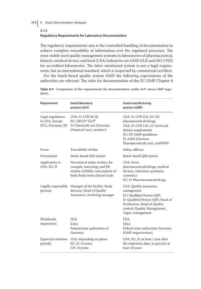
314 8 Smart Documentation Strategies

8.2.6Regulatory Requirements for Laboratory Documentation

The regulatory requirements aim at the controlled handling of documentation toachieve complete traceability of information over the regulated processes. Themost widely used quality management systems in laboratories of pharmaceutical,biotech, medical device, and food (USA) industries are GMP, GLP, and ISO 17025for accredited laboratories. The latter mentioned system is not a legal require-ment, but an international standard, which is inspected by commercial certifiers.

For the batch-based quality system GMP, the following expectations of theauthorities are relevant: The rules for documentation of the EU GMP Chapter 4

Table 8.4 Comparison of the requirements for documentation under GLP versus GMP regu-lation.

Requirement Good laboratorypractice (GLP)

Good manufacturingpractice (GMP)

Legal regulationsin USA, Europe(EU), Germany (D)

USA: 21 CFR 58 [5]EU: OECD “GLP”D: Chemicals Act (German:Chemical Law), section 6

USA: 21 CFR 210, 211 [6]pharmaceuticals/drugsUSA: 21 CFR 110, 111 food anddietary supplementsEU: EU GMP guidelinesD: AMG (GermanPharmaceuticals Act), AMWHV

Focus Traceability of data Safety, efficacy

Orientation Study-based QM system Batch-based QM system

Application inUSA, EU, D

Nonclinical safety studies, forexample, toxicology and PKstudies (ADME), and analysis ofbody fluids from clinical trials

USA: Food,pharmaceuticals/drugs, medicaldevices, veterinary products,cosmeticsEU, D: Pharmaceuticals/drugs

Legally responsiblepersons

Manager of the facility, Studydirector, Head of QualityAssurance, Archiving manager

USA: Quality assurance,managementEU: Qualified Person (QP)D: Qualified Person (QP), Head ofProduction, Head of Qualitycontrol, Quality Management,Upper management

Worldwideinspections

FDA FDAEMA EMAFederal state authorities ofGermany

Federal state authorities Germany(GMP inspectorates)

Expected retentionperiods

USA: depending on phaseEU, D: 15 yearsCH: 10 years

USA: EU, D: at least 1 year afterthe expiration date, in practice atleast 10 years

8.3 The Life Cycle Model for Regulated Documents in Practice 315

“Documentation” and “Computerized Systems” regulated in Annex 11 [7, 8]. Forthe United States, there is a special legal guidance that describes the expectationsof the laboratory records, 21 CFR §211.194 “Laboratory Records”[9], and 21 CFRPart 11 “Electronic records, electronic signatures”[10].

In general, specification and verification documents can be distinguished, whilein practice mixed forms of both document types exist. A typical specification doc-ument in the laboratory is a test specification, which contains all the requirementsfor carrying out the analysis starting with the mixing of solutions and reagentsto the calculation of the analytical results. As a typical example of a verificationdocument (record), a weighing record can be quoted. A mixed form of specifica-tion and verification documents is often found in test protocols that contain bothrequirements and relevant attestations [11].

In summary, the following requirements have to be fulfilled:The document control has to describe all activities of creation, review,

approval/authorization, distribution, modification and versioning, withdrawal,and archiving, and make it traceable for all quality review activities.

In practice, particularly records are subjected to a thorough review by a secondperson (four-eye principle), which proves the accuracy, completeness, andcompliance with internal and external requirements. For electronic data, besidesaccuracy, integrity, availability, and human readability have to be safeguarded(Table 8.4).

8.3The Life Cycle Model for Regulated Documents in Practice

The life cycle model of regulated documents officially starts with the planningof a document and ends with the withdrawal or deletion. Each individual docu-ment in the analysis process contributes to the traceability and quality of the result.Therefore, at least the following points need to be defined for each document (seeTable 8.5).

Once created by the author, reviewed by quality management, andreleased/approved by management, specification documents, for example,SOPs are valid. They are distributed to the area of application (scope), relevantpersonnel are trained and the document can then be applied. After application,the related verification documents are collected, organized, and relevant partsthereof are published, for example, a CoA as an extract from a set of data, whichin turn consists of a further set of raw data and meta-data.

Looking at this document life cycle from the perspective of a pure paper-drivenlaboratory, it can be seen that a significant amount of work is generated by thepurely manual execution of these steps. For organizations that already operate anelectronic document management system (DMS), there is the advantage that allsteps can be conducted highly automated and with a minimum of effort, that is,media breaks can be avoided, consequently.

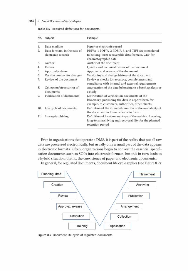
316 8 Smart Documentation Strategies

Table 8.5 Required definitions for documents.

No. Subject Example

1. Data medium Paper or electronic record2. Data formats, in the case of

electronic recordsPDF/A-1 PDF/A-2 PDF/A-3, and TIFF are consideredto be long-term recoverable data formats, CDF forchromatographic data

3. Author Author of the document4. Review Quality and technical review of the document5. Approval/release Approval and release of the document6. Version control for changes Versioning and change history of the document7. Review of the document Reviewer checks for accuracy, completeness, and

compliance with internal and external requirements8. Collection/structuring of

documentsAggregation of the data belonging to a batch analysis ora study

9. Publication of documents Distribution of verification documents of thelaboratory, publishing the data in report form, forexample, to customers, authorities, other clients

10. Life cycle of documents Definition of the intended duration of the availability ofthe document in human-readable form

11. Storage/archiving Definition of location and type of the archive. Ensuringlong-term archiving and recoverability for the plannedretention period

Even in organizations that operate a DMS, it is part of the reality that not all rawdata are processed electronically, but usually only a small part of the data appearsin electronic formats. Often, organizations begin to convert the essential specifi-cation documents such as SOPs into electronic formats, but this in turn leads toa hybrid situation, that is, the coexistence of paper and electronic documents.

In general, for regulated documents, document life cycle applies (see Figure 8.2):

Retirement

Archiving

Publication

Arrangement

Collection

ApplicationTraining

Distribution

Approval, release

Review

Creation

Planning, draft

Figure 8.2 Document life cycle of regulated documents.

8.4 Dealing with Hybrid Systems Comprising Paper and Electronic Records 317

8.4Dealing with Hybrid Systems Comprising Paper and Electronic Records

8.4.1Advantages and Disadvantages of Paper Versus Electronic Documents

This section describes the steps that are required to define an appropriate strategyfor dealing with mixed document systems (hybrid systems) of paper and electronicdocuments. Table 8.6 shows the advantages and disadvantages of using paper andelectronic documents.

In hybrid systems, time-consuming media breaks often cannot be avoided. Insome cases, electronic documents are printed, signed manually, scanned, andprinted out completely with the signature page again. This is classic duplicationof work, which could be avoided by using DMS.

Although for many years there are rumors about paperless offices and labo-ratories, it can be stated that more than ever paper is used for documentationpurposes. But the road is mapped-out: similar to the field of photography wheremost images are incurred nowadays in electronic form, more electronic data willbe generated and stored for regulatory purposes in the future. In principle, thesame requirements apply to electronic documents as to paper documents; how-ever, electronic documents have high demands for data security (see Table 8.6).In IT systems, access protection is ensured, for example, by user identity andpassword. Verification of the data integrity in IT systems can be performed veryquickly and efficiently by data integrity checks using checksums (e.g., md5).For example, it is possible to detect data corruption due to tampering or diskerrors.

Table 8.6 Overview of the dependencies of paper and electronic records.

Paper documents before archiving Electronic documents before archiving

• Only one original• Cost of distribution by copies• Great effort for change process• Paper distribution slow and laborious• Long search times• Cost- and space-intensive intermediate

storage

• High availability• Good integration• Searchability

Archived paper documents Archived electronic documentation

• Access security• Immutability• Recoverability• Technological independence• Manual authentication

• Data security (physical and logic)• Data integrity and data medium aging• Recoverability• Electronic authentication

318 8 Smart Documentation Strategies

The recoverability and readability of electronic data depends on two factors:

• hardware for reading the media and• software to ensure the readability of the data format.

On one hand, adequate reading devices must be available for this purpose, oth-erwise the data are worthless. On the other hand, suitable software must be ableto be make data formats readable.

If the primary electronic data (source data of the chromatograms) of a certainHPLC system exist in a vendor-specific (proprietary) format, sooner or later, themanufacturer will announce with a system update that the “old” data format is nolonger supported.

In principle, three scenarios are possible when it comes to the considerationof the long-term archivability and readability of previously collected electronicinformation:

a) Data are readable without converting (e.g., NetCDF as *.cdf files).b) Data can be restored only after conversion, which possibly goes along with a

small loss.c) Data are no longer readable after changing the hardware/software by the sup-

plier.

In case (a), the user would have no problem with the readability of the “old” data,because the new updated system (or a vendor-independent generic system) allowsthe recovery of data.

In case (b), the user has to conduct a data migration, according to a validatedprocedure.

In case (c), the data can no longer be restored in the chromatography datasystem (CDS) after an upgrade; this case can be compensated in severalways:

According to the FDA guideline “Scope and Application” published in 2003, it ispossible to delete the underlying original data in proprietary data format, if con-tent and meaning of the data are preserved and archived on a different platform(paper, vendor-independent electronic format, e.g., PDF/A-1).

… any copies of the required records should preserve their content andmeaning. As long as predicate rule requirements are fully satisfied and thecontent and meaning of the records are preserved and archived, youcan delete the electronic version of the records. In addition, paper andelectronic record and signature components can coexist (i.e., a hybrid sit-uation) as long as predicate rule requirements are met and the content andmeaning of those records are preserved … (citation from FDA directive“Scope and Application,” 2003) [12].

The PDF/A-1 format is according to ISO standard 19005 “Document manage-ment – electronic file format for long-term preservation” considered as long-term

8.4 Dealing with Hybrid Systems Comprising Paper and Electronic Records 319

Final report

Electronically signed and

transmitted to authorities

Result data including meta data

contain information

On operators, methods

Human readable

In case of system change/update

1. Data readable

2. Readable after conversion

3. No longer readable

Reports

(eCTD) Report

Processed data(Independentfrom vendor)

Proprietary data format

Secondary

electronic data

including

meta-Data

Primary

electronic

data

(e-Raw

Data)

Figure 8.3 Data model of instrumental raw data, calculated result data, and report data.

archivable format and thus provides an elegant way to avoid paper documents andinstead produce genuine electronic data that are independent of the manufacturer,for all applications that have been printed-out so far. AdobeTM has disclosed thisformat, so that this data format can actually be recovered in the future with anysuitable pdf-reader (Figure 8.3).

8.4.2Implementation Strategy

Based on the presented requirements and constraints, as well as the experiencesgained in practice, different approaches to the challenges of the integrated doc-umentation of paper and electronic records arise, depending on the technologylevel of an organization.

Three basic implementation strategies can be identified:

a) organization with focus on paper-based documentationb) organization with “isolated applications,” using hybrid systemsc) organization that is consistently aligned to integrated electronic solutions.

Strategy (a) represents the least sustainable model, because it consciouslyaccepts the fact that the documents archived in paper form, already exist in anelectronic format, and thus accepts media discontinuity, including high costs ofproduction, distribution, modification, cancellation, redistribution, archiving,and not least their recovery.

Strategy (b) is found in organizations that aim on automation in some areasand are already working with partial solutions such as LIMS, with or withoutonline instrument connections such as … “Enterprise Resource Planning” (ERP),

320 8 Smart Documentation Strategies

DMS, and ELN “Electronic Lab Notebook.” These solutions must be operated ina validated environment, resulting in a very high burden during the design andimplementation phases. In addition, a number of different electronic manufac-turer-specific data formats are created, besides paper documents.

Strategy (c), that is, the consistent focus on purely electronic documentation hasbeen realized only by a few companies. The benefits that result from this modeloutweigh the costs of implementation of such systems in a regulated environment.The consistent implementation of such systems includes the use of subsystems, aselectronic signatures that comply with regulatory requirements. The digital sig-nature must contain the following elements: the reason of the signature, date andtime, time zone, and the full name of the signatory.

The biggest initial gain in the transition from paper-based to electronicdocumentation can be achieved by laboratories that take the decision to converta paper-intensive process step into an electronic form. That means many com-panies opt for a gradual implementation in the form that the paper printoutsof chromatograms are replaced by PDF/A-1 files. So step by step, the singledocumentation steps are converted from paper to electronic format and inthe end will form an integrated solution that deserves the labeling “electronicdocumentation.”

8.5Preview

In fact, regulatory authorities responsible for pharmaceuticals and medicaldevices more commonly request electronic registration documents, and it can bepredicted that there will be no more traditional paper filings in the near future.First, for competitive reasons (time to market), and second due to time and costaspects, because the electronic versions of registration documents allow theauthorities representatives to copy and paste operations, search the documents,as well as analyze and integrate data by programs of the authorities.

It may be assumed for the future that owing to standardization of source data(NetCDF, *.cdf ) and availability of source data in the PDF/A-3 format, the authori-ties will not only look at chromatograms but also reanalyze the data, such as detec-tion or quantification limits to check or verify peak purity. In connection withaudit trails used in the laboratories, such submitted chromatograms are clearlytraceable and laboratories will be as transparent as never before.

The major disadvantages of “pure” paper solutions and hybrid systems demandfor greater efforts toward comprehensive electronic solutions and it is a matterof time until separate systems such as LIMS, with online device connectionERP, DMS, and ELN will be integrated. In my personal opinion, as there is aPDF-reader for documents, there will be a CDF-reader for chromatographic datathat makes chromatographic data independent of manufacturer, system, platformor age of the data, and allows chromatographic source data to be visible andprocessible.

References 321

References

1. Matthews, L. and Miller, T. (2000)ASTM protocols for analytical datainterchange. Journal of LaboratoryAutomation, 5, 60, http://jla.sagepub.com/content/5/5/60.full (accessed 28December 2015).

2. ASTM-Standard for exchange ofchromatographic data from variousmanufacturers, ASTM E1947 - 98 (2009)Standard Specification for AnalyticalData Interchange Protocol for Chro-matographic Data, http://www.astm.org/Standards/E1947.htm (accessed 28December 2015).

3. SIPOC-model, Description at http://en.wikipedia.org/wiki/SIPOC (accessed28 December 2015).

4. Information about PDF standardsfrom the Library of Congress of theUnited States, “Library of CongressCollections”: PDF/A-1: http://www.digitalpreservation.gov/formats/fdd/fdd000125.shtml; PDF/A-2: http://www.digitalpreservation.gov/formats/fdd/fdd000319.shtml; PDF/A-3: http://www.digitalpreservation.gov/formats/fdd/fdd000360.shtml (accessed 28 December2015).

5. 21 CFR 58 GLP http://www.accessdata.fda.gov/scripts/cdrh/cfdocs/cfcfr/cfrsearch.cfm?cfrpart=58 (accessed28 December 2015).

6. 21 CFR Part 211 cGMP http://www.accessdata.fda.gov/scripts/cdrh/cfdocs/cfcfr/cfrsearch.cfm?cfrpart=211 (accessed28 December 2015).

7. EU GMP Kapitel 4 Documentationhttp://ec.europa.eu/health/files/eudralex/vol-4/chapter4_01-2011_en.pdf (accessed28 December 2015).

8. EU GMP Annex 11 Computerized Sys-tems http://ec.europa.eu/health/files/eudralex/vol-4/annex11_01-2011_en.pdf(accessed 28 December 2015).

9. 21 CFR §211.194 Laboratory Recordshttp://www.accessdata.fda.gov/scripts/cdrh/cfdocs/cfcfr/CFRSearch.cfm?fr=211.194 (accessed 28 December 2015).

10. 21 CFR Part 11 Electronic Records, Elec-tronic Signatures, http://www.accessdata.fda.gov/scripts/cdrh/cfdocs/cfcfr/CFRSearch.cfm?CFRPart=11 (accessed28 December 2015).

11. Chemikaliengesetz 6. Abschnitt GuteLaborpraxis http://www.gesetze-im-internet.de/bundesrecht/chemg/gesamt.pdf (accessed 28 December 2015).

12. FDA Guideline(August 2003)Electronic Records – Scopeand Application, http://www.fda.gov/regulatoryinformation/guidances/ucm125067.htm (accessed28 December 2015).

323

9Tips for a Successful FDA InspectionStefan Schmitz and Iris Retzko

9.1Introduction

The US health authority Food and Drug Administration carries out domestic andforeign inspections to investigate whether an organization works in accordancewith the US law (Code of Federal Regulations, CFR) and international guidelines.For the production and control of classically and biotechnologically manufacturedpharmaceuticals, the American laws Current Good Manufacturing Practices inManufacturing, Processing, Packaging or Holding of Drugs: General and 21 CFRPart 211 cGMP Current Good Manufacturing Practices For Finished Pharma-ceuticals constitute the essential legal framework for manufacturers and testlaboratories.

For the handling of electronic records and the use of electronic signatures, thelaw 21 CFR Part 11 Electronic Records, Electronic Signatures applies. In addition,adherence to a number of guidelines is mandatory, concerning the development,manufacture, packaging, labeling, storage, logistics, and testing. In the course ofthe submission of a new product to the US FDA, all participating companies andcontractors must be inspected for compliance with these laws and regulations.In this case, all companies involved in the filing, for example, sponsors, contrac-tors, contract manufacturers (Contract Manufacturing Organizations, CMOs), orcontract laboratories (Contract Research Organizations, CROs) have to pass a suc-cessful inspection, regardless of where in the world the service is provided.

The FDA inspectors, so-called FDA Investigators perform the inspection on thebasis of internal FDA procedures, the Compliance Program Guidance Manuals.Inspections of finished medicinal products for example are carried out accord-ing to the CPGM 7356.002 Drug Manufacturing Inspections and inspections priorto approval follow the CPGM 7346.832 pre-approval-inspections. It falls to eachinspector or team of inspectors, as well as the District Office in conjunction withthe Office of Regulatory Affairs (ORA), which inspection approach is followed.This depends, among other things, on the education and qualifications, experi-ence, the training received, and the relevant preference for certain core issues andcannot be predicted.

The HPLC Expert: Possibilities and Limitations of Modern High Performance Liquid Chromatography,First Edition. Edited by Stavros Kromidas.© 2016 Wiley-VCH Verlag GmbH & Co. KGaA. Published 2016 by Wiley-VCH Verlag GmbH & Co. KGaA.

324 9 Tips for a Successful FDA Inspection

Usually, two inspectors perform a preapproval inspection (PAI), but it is verycommon in recent times that only one experienced person takes over the entireinspection, especially when follow-up inspections are conducted. Is there a teamof two inspectors (female or male), one is usually responsible for the inspection ofthe quality systems, the other for the technical and scientific aspects.

Usually, the inspectors stay abroad for 3 weeks, and perform inspections at threeto five different organizations. A primary source of information for foreign inspec-tors regarding inspection regulations is the inspection manual Investigation Oper-ations Manual 2014. Another important basis for aspects of traveling is the Guideto International Inspections and Travel, updated version 2009.

Manufacturers and subcontractors (CROs, CMOs) that produce for the US mar-ket are obliged to register1) with the FDA and to disclose the activities related toproduction and testing. It is important for the inspection activities of the FDA thatall companies are listed in the FDA database with accurate, complete and cur-rent information. Besides other information, the company name, company size,address, business activities, and the inspection status are recorded. Almost everyFDA inspection includes the clarification of the registry and if it is not alreadydone, it is required to start the registration process during the inspection. Otherimportant functions of the FDA database are to inform politics and the publicabout the type and number of regulated companies and create budget plans forvarious compliance programs. A public database of the FDA for the represen-tation of registered companies2) is available to all interested parties. Here, thecompany name, the FEI number Firm Establishment Identifier, the DUNS numberData Universal Numbering System, address, and topicality of registration can beaccessed.

As part of the preparation, it is important to clarify with the FDA, and/or licens-ing partners, customers, which products are focused by the planned inspection toenable concentrated preparatory activities on these product(s). In the case of aninitial inspection, besides the inspection of the product-related issues, a generaland coherent good manufacturing practice (GMP) inspection is carried out in thetarget organization. This may well mean that other areas that are regulated by theAct 21 CFR 211, are inspected, because the inspection focuses on all products orprocesses potentially destined for the American market.

9.2Preparation with the Inspection Model

To support the preparation of an FDA audit in the laboratory, it seems reasonableto use a structured inspection model (see Figure 9.1), which categorizes the topicsto be inspected, and it allows to distribute the work packages to several projectmembers. All elements of this model have potential influence on the product andresult quality and are, therefore, critical to the safety and efficacy of the product.

1) http://www.fda.gov/ICECI/Inspections/FieldManagementDirectives/ucm096034.htm.2) http://www.accessdata.fda.gov/scripts/cder/drls/default.cfm.

9.2 Preparation with the Inspection Model 325

Key systems

1. Material system

2. Facilities and equipment

3. Laboratory control system

4. Training

5. Quality system

6. Document control / records

Critical elements

Change control

Deviations

OOS (out-of-specification) and

CAPA (corrective and preventive action)

Training

Figure 9.1 Inspection model for structuring the topics.

For understanding the key relationships and to explain complex issues, it isadvantageous to create a historical overview of the projects and products thatshows who have worked together at what time with which partners to develop,manufacture, store, process, or test the product. Sometimes, it is also necessaryto de-archive older documents to be able to clarify historical facts. Sometimes,personnel, who were significantly involved in the project in the past, are no longeravailable, so that this historical analyses are of particular importance.

9.2.1Materials, Reagents, and Reference Standards

This includes all incoming goods, materials, reagents, solutions, referencestandards, and mobile and stationary phases that are relevant for the product ofinterest. The material flow, warehousing, containers used, labeling, testing, orthe establishment of shelf-lives are typical questions on this group of themes.Furthermore, the concepts of identification, labeling, and traceability have to bemade transparent, from delivery to usage or disposal. All software systems thathave to do with the identification, registration, storage, redistribution, are subjectto inspections that aim to prove the suitability of these systems (validation).

Case 1 Box: Practical Tips on the Subject: Materials, Reagents, ReferenceStandards

• Delivery notes of materials received shall be provided on request.• Goods receipts are clearly documented (paper and/or electronic version).• All reference substances are tested for validity, certificates are complete, and

invalid substances are removed.• Material safety data sheets are available for all reference substances.• Mixed solutions, reagents, and mobile phases are clearly documented; all

used test equipment such as balances, pipettes, refrigerators, and freezersare identified and calibrated.

• Reagents, solvents, and mobile phases are controlled regarding expirationdate and replaced if necessary, including laboratory water and othersolvents.

326 9 Tips for a Successful FDA Inspection

• Samples, reagents, solvents, and mobile phases on laboratory benches andshelves are labeled clearly and in accordance with (legal) requirements.

• Samples and specimens in refrigerators and freezers, are checked, forexample, for expiration date, clear labeling.

• Labels on solvent and reagent flasks are as specified, for example, not man-ually overwritten.

• Reference standards of the US Pharmacopoeia (USP) must be used, even ifthere are other alternatives.

9.2.2Facilities and Equipment

For analytical instruments of a quality control laboratory, which are under GMPgenerally referred to as equipment, the evidence of qualified operation, qualifi-cation, and, for computer-based systems, a validation, have to be provided. Theequipment, facilities, and systems must be described by appropriate system doc-umentation and it is expected that in the vicinity of the system a system binder andlogbook provide information on the qualification and/or the calibration status. Ingeneral, inspectors ask about the frequency of calibration intervals, the accompa-nying documentation, and the training of responsible personnel (system owner,equipment manager). If changes of the test equipment are carried out, this shouldbe documented as part of the controlled change management (change control).It is useful to categorize the equipment according to chapter <1058> AnalyticalInstrument Qualification of the USP:

A: Exempt equipment, such as magnetic stirrer, vortex mixer, calculators, LCDtimer.

B: Calibrated equipment, such as balances, pipettes, pH meters, refrigerators,and freezers.

C: Computer-based systems, such as modular or compact HPLC instruments,spectrometers.

Case 2 Box: Practical Tips on the Subject: Facilities and Equipment

• Access controls for the building and all relevant subcompartments areenabled.

• Laboratory coat is worn; safety glasses are carried in the jacket pocket andworn where required.

• Visitor coat and glasses are kept ready for the inspectors.• Hygiene requirements (e.g., cleanroom locks, disinfection) also apply for the

inspectors.

9.2 Preparation with the Inspection Model 327

• All equipment binders/logbooks are checked for good condition and main-tained up to date.

• A validation master plan that contains concepts of qualification, re-qualification, risk assessment, validation, maintenance, periodic inspections,and system retirement is kept.

• All laboratory equipment is included in an inventory list that has at least thefollowing attributes: device ID, location, person responsible for the equip-ment, purpose of use, reference to SOPs.

• Lab equipment is categorized according to USP <1058> into three classes(A, B, C).

• Qualification status of the relevant equipment is checked.• Calibration and maintenance status (SOP) of the relevant equipment

is checked, which also includes refrigerators, freezers, drying ovens,incubators, balances, dilutors, pipettes, and so on.

• For computerized systems, risk-based validations are available that coveraccess controls (data security), audit trails, viewing the data formats,recovery, handling in case of failure, backup and archiving, data integrity.

• Calibration documents of reference equipment are maintained.• The person responsible for the equipment is able to present clear audit trail

functions and records for a past time period on the screen.• The screen-lock is active or a password-protected screensaver is set automat-

ically after a defined time (e.g., company logo as screensaver).• Equipment that is expired or no longer in-use is labeled as “Rejected” or qual-

ified before the inspection.• It should be possible to retrace and explain recent as well as former changes

(Change Control).• The persons responsible for equipment are trained for the presentation of

important laboratory equipment (e.g., HPLC, balances, pipettes, pH meters,refrigerators).

• Wastepaper baskets are emptied to avoid discussions about raw data dis-posal.

The persons responsible for equipment have, in this part of the inspection, theimportant role of demonstrating to the inspectors that all significant aspects ofGMP are under control. The persons responsible for equipment have to fulfill thefollowing essential tasks:

1) Documented briefing and training by the supplier (“in-house expert”)2) Issue of an SOP for operation, function testing, calibration, maintenance and

cleaning of the equipment3) Issuing and maintenance of an equipment logbook to document relevant

events during the life cycle4) Responsibility for periodic functional tests and calibrations5) In-house training and documentation of additional equipment users

328 9 Tips for a Successful FDA Inspection

6) Updating of qualification documentation after modifications and repairs7) Definition and training of a representative8) Closure of equipment in the case of a violation of acceptance limits9) Ordering and stocking of important consumables and spare parts

10) Presentation of the equipment during audits and inspections.

In practice, it is important that the responsible persons can perform these top-ics using work instructions and that the operation is compliant with establishedprocedures (SOPs). It is not unusual that FDA inspectors interview two personsabout the same issue (investigative interview), and observe real laboratory opera-tions on site.

9.2.3Laboratory Controls

The testing of incoming goods, intermediate materials, packaging, in-process con-trols, and final release are tasks of the test facilities, such as the quality controllaboratories. The tests shall be carried out by validated methods, especially in laterphases or shortly before regulatory submission. The method validation shouldbe planned, conducted, and documented in accordance with the guideline ICHQ2 (R1): Validation of analytical procedures: Text and Methodology. All relevantmethods should be checked for their validation status, as well as their validity.Method development, validation, and transfer generally have a high priority inFDA inspections. It is advisable to list the method development, the resulting val-idated methods and versions to make a historical comparison of the respectivevalid specifications so that in case of doubt, it can be shown at any time, whichmethod has been used in which validation status for testing against a specification.Further assistance can be provided by the FDA guidance Analytical Proceduresand Methods Validation (2000), which gives valuable information on the expectedtype of documentation for analytical methods.

Transfers of analytical methods are also evaluated very critically, and analyti-cal transfer plans with defined acceptance criteria are expected, as well as relatedtransfer reports. On this topic, the USP <1224> Transfer of Analytical Proce-dures offers some guidance. For assistance on the confirmation of pharmacopoeiamethods, the chapter USP <1226> Verification of Compendial Methods can belooked up.

Case 3 Box: Practical Tips on the Subject: Laboratory Controls

• The test specifications are saved in the instrument method of the measuringequipment and can easily be identified by an ID or a homonymous name.

• Instrument methods must be identical to paper-based version.• The current test procedure is located near the workplace.

9.2 Preparation with the Inspection Model 329

• All samples in the autosampler of the HPLC are listed exactly in the order ofthe analysis sequence and include system suitability tests (SSTs) and calibra-tion samples.

• Samples that are no longer needed (elapsed) in the autosampler areremoved.

• The validation documents for the relevant methods are available in writtenform, are signed, and comprise a validation plan and report.

• The corresponding raw data undergo a meticulous review, during prepara-tion phase.

• Key elements of a validation should be documented by raw data, forexample, robustness, with respect to pH of the mobile phase, the mobilephase composition, the shelf life of reference samples, and the columntemperature.

• If the method is stability indicating, this should be demonstrated by stress-test data, measured during method-development.

• The essential data for complete traceability (who, when, what, how, what,where?) are documented on the printouts of the analytical results.

• Work instructions for all aspects of stability testing are available (e.g., plan-ning, logistics, implementation, evaluation, qualification of stability storagecabinets, respective storage rooms).

• Written stability-testing protocols are available for all relevant tests. They aredated and signed.

• If manual integrations are performed in automated data analyses, they haveto be conducted according to a current procedure. If only manual integra-tions will be applied, this has to be described as well, using illustrated andcomprehensive examples.

• Ensure that all essential calculations are reviewed by a second personto ensure accuracy, completeness, and compliance with the applicableregulations, and that this procedure is regulated and documented.

9.2.4Personnel

The training of staff is an important element of compliance with legal andself-imposed quality standards and is based on the education and qualification ofa person, considering the dedicated job profile. It is expected that the companyconducts training plans for employees who are subjected to regular target-performance comparisons, to continuously determine the training status. Thetrainings regarding the GMP requirements have to be carried out periodically andshould be documented. A proof of the training success is also currently expectedby the inspectors. For persons who are engaged for a long time in an importantfunction, but do not have a training certificate for their activities, a document

330 9 Tips for a Successful FDA Inspection

should be created that attests these many years of experience as training on thejob to provide a training record for the inspection. This training record should besigned by the person, line manager, and quality management.

Each employee should take the responsibility to update his/her training recordsand should know where the training records are kept, as part of the inspectionpreparation. A chronological list of all internal and external trainings and therespective training certificates should be available at a central location. For allkey personnel, an updated job description should be available, describing theactual tasks correctly and completely. The individual job description shouldbe known precisely by each employee, because inspectors often ask peopleduring their company-walkthrough about their job profile or what they are doingcurrently.

Case 4 Box: Practical Tips on the Subject: Personnel

• A training plan for the employees is available and is updated.• Each employee should review his/her training records, regarding, for

example, vocational education and training, GMP training, and update asappropriate.

• Job descriptions for all key personnel are in an updated form and reflect theactual responsibilities of each employee.

• For groups of employees function-related collective job descriptions may bedefined.

• Annual GMP refresher-trainings are conducted.• Specific trainings are available for all testing activities (test procedures,

equipment training).• Trainings of employees who were absent for a longer time, for example,

maternity leave, have to be refreshed upon come-back.• Each employee catches up on his/her current job profile before the inspec-

tion and can also reflect it.

9.2.5Quality Management

The Quality Management department is expected to carry out regular target-performance comparisons of specifications and requirements, document theevaluations, and provide management with information on the results. For allpossible discrepancies from the desired state, for example, complaints, results outof specification (OOS), changes, deviations, and audit results (internal and exter-nal audits), the appendant information are collected centrally and processed bymeans of the Corrective And Preventive Action (CAPA) system. These monitoringand control functions are performed by the staff of quality management.

9.2 Preparation with the Inspection Model 331

It is very likely that during the inspection historical events of the above-mentioned topics will be surveyed and it is expected that the involved personshave evaluated the processes with scientific expertise and appropriate riskassessments. A controlled, informed, and trained handling of these critical issuesis mandatory. Compliance with set review-cycles for specification-documentswill be checked randomly and should be considered in the preparation phase ofthe inspection.

Eventually, it should be paid attention to documentation in paper and electronicform, according to 21 CFR Part 11. Often a combination of paper and electronicrecords (hybrid solution) is used in companies and it has to be decided case bycase which type of document is stored in which system. For important electronicsystems, it has to be determined, for example, which data format is used, how thedata retrieval over the retention period can be ensured (data format, data reliabil-ity, data integrity), and how the document has been authenticated.

For many inspectors, the assessment of the project or product documentation,in conjunction with the contractual agreements between sponsor and contractor,is an important element of compliance. Thus, the involved departments, particu-larly the purchasing department, research and development (R&D), quality con-trol and, where appropriate, the production as well as critical suppliers shouldbe involved in the review of these quality and service agreements. Agreementsmade earlier should be checked for up-to-dateness and specifications. Especiallyfor critical suppliers, this review is of great importance, as it assures the validityand compliance with the agreements. Particular focus is set on the communica-tion between the involved parties. The FDA is aware of the fact that there arecommunication problems in many cases between the parties, so that sufficientattention should be paid to the correspondence and/or telephone notes, becausesome important decisions in the project can be best documented by an e-mail, awritten note, or the signed phone minutes of a conference call.

The different departments should verify the applicable parts of the registrationdossiers and related documents and records for accuracy, completeness, and con-sistency. This ensures that there will be no surprises during the FDA inspection,which could lead to agitation and discussions.

Case 5 Box: Practical Tips on the Subject: Quality Management

• There is a list of all standard operating procedures (SOPs).• The SOPs governing the activities of the QM department, are updated, valid

and trained.• All SOPs on the topics “change control” (Change Control), “deviations”, “re-

sults out of specification” (OOS), “corrective and preventive actions” (CAPA),as well as “training” are updated, valid and trained.

• Self-inspections are planned and conducted as scheduled.• Supplier inspections are planned and conducted according to plan.

332 9 Tips for a Successful FDA Inspection

• Management reviews are carried out regularly and are documented.• The job descriptions of all QM staff are available and updated.• Lists of complaints, results OOS, deviations, and changes for the product that

is in the inspection-focus are available, covering the past 24 months.• For deviations from the past that have not been addressed satisfactorily,

review-documents with conclusive explanations and consequences areavailable.

9.2.6Documents and Records

Documents and records are the most important issue in FDA inspections, due tothe irrefutable principle “What is not documented, is not done!” a fundamentaldifferentiation is made between specification documents (e.g., test procedures)and verification documents (e.g., test protocols and laboratory records). Moreinformation is available in Chapter 8.

Case 6 Box: Practical Tips on the Subject: Documents and Records

• All standard operating procedures (SOPs), specifications, manuals, andinstructions are available in the specified binder in the laboratory; checkwith table of contents, all documents up-to-date.

• Documents related to deviations, changes, OOS results, complaints, andCAPA are stored and managed centrally by the QM.

• All laboratory notebooks and worksheets are checked by a second employeewith initials and date (accuracy, completeness, compliance), according to 21CFR 211.194 (Lab Records).

• No self-adhesive labels (post-its) are used in the laboratory, even for privateinformation.

• Blotting pads are blank, no calculations on calendar sheets.• Wastepaper baskets are emptied; no raw data, chromatograms, or reports

(even drafts) in the bins.• No weighing printouts lying around on the balance printer or near by.• All data storage media such as floppy disks, CDs, DVDs, memory cards are

placed inside the drawers, because usually they are not labeled sufficiently.• Binder labels should be uniform and appropriate to regulations (e.g., colors).• Older versions of documents are removed from the laboratory.• No handwritten entries in specification documents (SOPs or similar).• Handwritten entries, for example, in verification documents only with indeli-

ble pens (DIN ISO 12757-2).• No use of thermal paper and ink-jet printing for archival purposes.

9.3 Typical Course of an FDA Inspection 333

• An archive is established and meets all the criteria of protection against fire,flood, and other catastrophic data loss.

9.3Typical Course of an FDA Inspection

FDA inspections follow a typical course, which has developed in practice as thestandard sequence (see Figure 9.2).

Once the inspectors have entered the audit room, they are greeted by the repre-sentative of the management. Then, the exchange of business cards and personalpresentation follow. The other participants introduce themselves as well as themanagement representative and hand over their business cards. This usually hap-pens before the inspectors have taken a seat. After the inspection, the businesscards are a valuable source of information on names and functions of the contactpersons who participated in the inspection. It is common that the inspectors iden-tify themselves to members of management with their identity card “credentials”and thus begin the official part of the inspection.

Participants of the “opening meeting” are compiled from the persons in theaudit room, back office, and other interested or maybe involved persons from thedepartments. The FDA inspectors are quite used to a larger number of participantsin opening meetings. If the number of seats is limited, at least the persons directlyinvolved in the audit room and the back office should take part in the opening

Preparing audit

room and

backoffice

Full-scale

preparation phaseTrip coordination

and

communication

Inspection

announcement

Exit meeting

Day 1

Continuation

of inspection

Discussion of

observations

Inspection

result

Closeout

meeting

Day 1

inspection

Opening

meeting

Company

presentation

“Walk

through”

Review of

documents

InterviewsReview of

systems

Approximately 6 weeks before inspection

Figure 9.2 Typical course of an FDA inspection.

334 9 Tips for a Successful FDA Inspection

meeting. If the room size is sufficient 10–20 persons may participate. The open-ing meeting offers the opportunity for all participants to get a first impression ofthe inspectors. If the inspectors have taken a seat, the representative of the execu-tive board should obtain permission from the inspectors to show a short companypresentation, which is almost always accepted.

The company presentation for the opening meeting should be created and pre-sented in English, and the inspectors should be provided with a printout so thatthey can take notes for future reference. Later, it facilitates writing of the reportfor the inspectors.

The contents of the company presentation are intended to familiarize theinspectors with the basic facts of the company in a short time and to give them afirst impression of the organization. It is important that the presentation does notoccupy too much time. Typical times are between 15 and 30 min for the entirecompany presentation. The presentation can be conducted by several persons,but it makes sense to limit the number of presenters on two or three. For example,the general part could be presented by a management representative, the historyof the product, the associated contractors and processes by the product manageror head of Regulatory Affairs, and the part that deals with quality managementby the head of Quality Management.

Case 7 Box: Company Presentation

• Overview of the company’s name, affiliated group, headquarter, location(s)• Overview of the economic indicators, number of employees, and so on• Overview of the main products and markets, related to the US market• Overview of the product focused by the current inspection, with information

on history, processes, techniques, locations, subprocesses, key suppliers, orsubcontractors, for example, sterilization process

• Organizational chart of the group, the location, the departments that arefocused by the FDA, for example, QM, R&D, production, packaging, qualitycontrol laboratory

• Location plan; inspection relevant buildings should be marked• Floor plans of essential facilities such as production, packaging, storage,

quality control, laboratory• Presentation of the audit core team (persons in the audit room are direct con-

tact persons during the inspection)• Presentation of the quality systems established on-site (e.g., ISO 17025, cGMP

21 CFR 211), with a short historical overview• Information on audits of authorities (brief history and current inspection sta-

tus, accreditations, and certifications)• Information about any previous FDA inspection (on-site)• Information on the integration of Quality Management into the value chain

(opportunity to present the QM as an integral part of the company processes)

9.4 During the Inspection 335

• Brief overview of the documentation systems of the company, for example,QM manual, process instruction (PI) sheets, test procedures and associatedprotocols, operating procedures (SOPs).

Immediately after the company presentation, the inspectors should be invitedto ask questions. When all questions are answered, the lead inspector will intro-duce the team and reveal the contents of the inspection. This should bring nosurprises, because already in the preparation phase of the inspection, it is of theutmost importance to strictly clarify the scope of the upcoming FDA inspection.

After agreement on the contents of the inspection, a little break to drink coffee,tea, or soft drinks can be used to give the participants who do not belong to thecore team of the audit room, the opportunity to leave the room.

In most cases, the inspection begins with a company-walkthrough, which mayinclude the usual areas such as incoming goods area, warehouse, product testing,quality control laboratories, manufacturing, packaging and storage, and logistics.It is difficult to predict which systems are studied in the first step, because thecompany-walkthrough serves to form a first overview of the company and it maywell be that the tour will be continued later or on the following days.

9.4During the Inspection

The “audit room” is the room, in which the inspectors and the core team stayduring the inspection and where the documents and records are reviewed by theinspectors. This is also where the opening meeting and the “closeout meeting” takeplace. The management or management representatives must be present both atthe beginning and at the end of the inspection.

The following requirements apply to the audit room:

• Room with good indoor climate (air conditioning in summer, heating in winter,natural light as possible and windows)

• Sufficiently large workspace on the tables, so that documents can be well spread• Sufficient number of seats for the participants• Ideally, for the opening meeting and the closeout meeting room for more par-

ticipants should be provided.

Who should be in the audit room?

• Inspectors (typically, one to two persons)• Management (only for welcome and farewell of inspectors)• Head of quality management as the main contact person• Representatives of the regulatory affairs department (optional)• Note-taker and Moderator, usually in one person• Interpreter(s), if this option is selected

336 9 Tips for a Successful FDA Inspection

• Two vacant seats for persons, who have to present results or documents (e.g.,manager and employee).

Lists in the audit room:

• Audit room protocol (paper or better: intranet based, online connected withback office)

• List of participants (registration of all participants in order of occurrence afterthe beginning of the inspection, including name, position, topics discussed)

• Audit room tracking list (document for tracking the documents that come fromthe back office into the audit room, including comments on the status of thedocuments and whether the documents have been reviewed or copied and takenby the FDA inspectors).

The “back office” is the communication center in the background of an FDAinspection. Here, all information from the audit room about the questions orneeds of the inspectors is gathered. These requests can be reported to the backoffice, either directly from the audit room or during the company-walkthrough.All documents, records, or samples requested by the inspectors shall be verifiedfirst in the back office and then transferred to the audit room. Similarly, thepersons who have to present issues of their field of responsibility in the auditroom will be prepared in the back office (briefing). These persons are kept readyand wait in the back office until they are called by the note-taker of the audit roomto present their topic. These activities are to be documented by the note-taker inthe back office tracking list.

The following requirements apply to the back office:

• Room situated within walking distance to the audit room (not more than1–2 min foot-walk)

• Sufficiently large work surface on tables, so that documents can be well spread• Sufficient number of seats for the team and persons waiting to be called to the

audit room• Space for the binders that are needed for the audit.

The technical equipment should enable network connections to access impor-tant documents (e.g., SOPs, process instructions, and manufacturing and test doc-uments), records, journals, guidelines, or pharmacopoeias (e.g., USP). Internalroles and responsibilities as well as contact persons should be defined individ-ually for each FDA inspection, as this may change due to the inspected issues. Theback office administrates the “document tracking list,” which contains the statusof all requested documents.

9.4.1Behavior in Inspections

In general, the selection of persons who have direct contact with the FDA inspec-tors should consider that the following skills are well developed: balanced mood,

9.4 During the Inspection 337

unexcited style of discussion, structured logical thinking and working, strong ser-vice orientation, stress resistance, general overview, and adaptability.

For the dress code, there is only one rule: You should feel comfortable in yourclothes. Not too formal – not too casual, but comfortable and customary clothesthat do not overly exceed the level of the inspectors’ clothes. If you generally donot wear a neck-tie, you should not wear it in the inspection. Women should avoidshoes with very high heels and use decorative cosmetics, accessories and jewelrywith restraint.

The inspectors are usually addressed by first-name, if he or she does notpresent and behave in a very formal way. This is common in the United Statesand, however, should not be interpreted as a chummy form of address (as itmay imply for Europeans). It should be remembered that the inspection is aformal administrative act, similar to a tax audit or judicial investigation, despitethe relaxed and casual appearance, or speech of the inspectors. Monitor thesituation thoughtful and focused, and try to help the inspector to make his or herwork as comfortable as possible. The general behavior should be characterizedby friendliness and commitment, because people from the American cultureare accustomed to a friendly and open environment. A natural smile or friendlygesture is the best guarantee that you will reach the “human touch” of theinspectors.

The form of address of your managers, colleagues, and subordinate employeesshould be retained, as it is customary in your company and in the individual rela-tions: If you generally address by first-name, you should also do it in the inspectionand the same when you generally use the more formal surname.

All inspection participants with direct FDA contact should be trained for theinteraction with the inspectors, so that the chances of a successful communicationincrease. It has been proven in practice that it is helpful to observe the followingpoints.

Case 8 Box: Practical Tips on the Subject: Behavior in Inspections

• Be friendly, relaxed and concentrate on the statements and questions of theinspectors.

• Make use of simultaneous interpreters, if you do not feel comfortable inEnglish, because the inspection language is always English.

• All statements you make must be supported by a written evidence, forexample, a test procedure or method, a standard operating procedure(SOP), or a technical test report.

• All of the statements you make must be honest and reflect the facts as com-pletely as possible.

• Answer only the question with a precise response, without further embel-lishments or details that you plan for the future.

• If you do not understand the question, ask for repetition of the question.

338 9 Tips for a Successful FDA Inspection

• Be responsive to “small talk” offers of the inspectors, for example, on topicssuch as weather, culture, regional points of interest or culinary specialties,travel, history, countries, and customs, because that relaxes the atmosphere.

For the successful presentation of your position, it is important to be on a parwith the inspectors. This means that you should neither present yourself techni-cally more competent or superior, nor behave like you are in a weak position, orfeel attacked and adopt a defensive position. If you do not succeed in presentingyour compliance convincingly in some cases, remain calm and offer to procureadditional data and facts from the back office, which can provide further clarifi-cation. If this additional information cannot be brought in a timely manner, ask(usually the note-taker or moderator) to shift the issue to a later point of time.Longer pauses and silence of the inspectors should not unsettle the core team, butare seen as a normal part of such audits.

9.4.2Lab Walkthrough

As already mentioned, a laboratory-walkthrough is usually conducted immedi-ately after the opening meeting. It may be that the inspectors plan the route withyou, or join your proposed route. Eventually, it is irrelevant who proposes theroute, because inspectors are trained to enter the essential premises and to con-duct their investigations.

If there are two inspectors, it must be expected that the group splits, whichshould be considered as an option when planning the escort of the inspectors.Some inspectors inspect according to the material flow and track the full path ofthe testing procedure, but there are also some who take a seemingly arbitrary wayand change from one topic to the next during their lab-walkthrough. The employ-ees in the different areas of the company should continue to work normally, asif it were an ordinary working day, even if the FDA inspectors approach. Onlyon request, people should speak with the inspectors, otherwise continue to workroutinely.

In general, as few persons as necessary shall accompany the inspectors on thecompany tour. In any case, the escort should include the head of quality manage-ment, a note-taker, a representative of each visited department, and a “stand-byperson,” who may bring documents and records, if the employees of the depart-ment are currently occupied by the questions of the inspector.

9.4.3The Inspection in the Audit Room (Front Office)

Most of the inspection time is usually spent in the audit room. The atten-dees shall deliver documents, records, procedures, and processes, on request

9.4 During the Inspection 339

of the inspectors. While preparing the audit room a suitable place for theinspector(s) should be selected. It should be selected the best possible andcomfortable place with sufficient lighting and no passage door behind thechair.

Documents are generally presented in the original form. In case the inspectorslike to take along certain documents, they should be copied and stampedas confidential information so that the information cannot be disseminated.Under the FOI Freedom Information Act of the United States, informationfrom FDA 483 forms and warning letters are accessible to the public via theInternet.

All records and documents that are related to regulated processes and productsmay be requested by the inspectors (see IOM, 2015, Chapter 5.6.2.3 – Records).However, the FDA exercises restraint with regard to the examination of internalaudit reports or supplier audits. The FDA inspectors are entitled to demand andtake samples, specimens and reference materials from the inspected company. Therequired samples shall be documented in a list and handed over to the inspector(see IOM, 2011, Chapter 5.10.4.3.17 – Samples Collected).

9.4.4Dealing with Obviously Serious Observations

If there is a significant and serious observation, remain calm and friendly asit could be that additional data could clarify the situation. Therefore, ask for apostponement of the question until you can provide further data. However, youshould not do this to fend off the question, but with the intention to supportthe inspector as best you can and help him or her with the investigation of thefacts.

Use the gained time in the back office, involving all persons, who are able to con-tribute to the clarification and try to develop a conclusive answer. If you are unableto convince the inspector, please explain the circumstances on the basis of factsand mitigate the original observation by relativizing statements that are supportedby facts. In practice, a three-step process for dealing with difficult observations hasproved to be effective:

1) Agree to the obvious findings (honesty).2) Provide additional information to clarify (relativization).3) Describe procedures that will prevent such events in the future (CAPA or

PACA, sometimes it depends on the order of corrective and preventive mea-sures).

With the method described here, deficits can be dispelled, especially deficitsfound prior to the inspection by internal or third-party reviews and make them“harmless” for the FDA inspection. Experience reports that comprise a descriptionof deficits, relativizing facts and appropriate CAPA are suitable tools to process thethree-step method.

340 9 Tips for a Successful FDA Inspection

9.4.5Documentation of Observations on Form FDA 483

If an observation is recorded on FDA Form 483, you have the opportunity toaddress and discuss this issue on each inspection day in the exit meeting. However,new data and additional information must be provided that was not available atthe time, when the observation was made. Take advantage of the openness of theinspectors to discuss. Please keep in mind that for the inspectors the foreign envi-ronment and language are stressors and apply social and intercultural sensitivityin order to determine how far you can go in the discussion.

The opportunity of clarifying and possibly discussion of factual open questionsor observations should be used in a short exit meeting on each inspection day bythe core team in the audit room. All issues that can be solved on site should beaddressed on site, because usually it is difficult to convince the FDA district officewith written statements on complicated facts, after the inspection. Most investi-gators are very well trained and experienced, so that discussions with a technicalbackground can be performed thoroughly. Again, the communication shall bevery friendly and factual. It cannot be emphasized enough that the inspectors aretrained to discuss the results of the FDA 483 observations and your proposed cor-rective actions (see IOM, 2014, Section 5.2.3), so you should use this opportunityduring the inspection.

At the end of each day’s “exit meeting,” it should be asked what subjects areplanned for the following day of the inspection, since the evening is still availableto prepare essential things, such as translations of relevant texts into English, ifdesired, or to make graphical representations that can contribute to clarificationand transparency. The agreement of a provisional agenda for the following daysignificantly facilitates the entry into the new inspection day and should be usedas an opportunity.

In the final meeting of the FDA inspection, the closeout meeting, the presence ofa representative of the management is mandatory. If there are any observations onForm FDA 483, the inspector is obliged to hand over this document to the man-agement representative personally. At this meeting, there should be no surprises,as all observations have already been presented in the daily “exit meetings” on theprevious days, and possibly were discussed. If no final agreement could be reachedfor an observation, the possibility of an Annotation to the FDA 483 observationscan be used. If there are no FDA 483 observations on the form the meeting willbe terminated quickly, while in the case of observations all violations will be readaloud. The observations are presented at this time without citation of the rele-vant legal text. The exact quote is created later by the District Office in the UnitedStates and is listed explicitly in the report of the inspector, the EIR EstablishmentInspection Report.

The final report EIR is written in English (see IOM, 2014, Chapter 5.10.4) andusually follows 6–12 weeks after an inspection. The EIR contains• printout of FACTS “Facility Establishment Inspection Record”• acknowledgment statement (“endorsement,” discussed later)

Further Readings 341

• a copy of the FDA Forms FDA 482, FDA 483, and FDA 484• summarized report of the inspector• copy of the inspection mandate, if available• exhibits and finds that are described in the report• checklists, for example, BSE Checklist• the original checklists should be handed out with the EIR.

9.5Post-Processing of the Inspection

The FDA Form 483 is used to log the observed GMP violations found by inspec-tors during the stay in the company (IOM, 2014, Chapter 5.2.3. seqq.) In princi-ple, these observations are the result of subjective perceptions of the inspectorsand can be based on misunderstandings, not fully clarified facts or faulty com-munication. However, there can be justified objectively measurable facts that areconsistently seen by inspectors and inspected company.

Once an FDA Form 483 signed by the inspector is handed over to the man-agement, only the written path can be taken to comment on the observations,to relativize, and to make suggestions for corrective and preventive measures. Theexpectation of the FDA is that 483 observations will be answered in writing within15 working days.

If there are observations on the FDA Form 483, those persons involved in theinspection should be consulted that have detailed knowledge about how it came tothis observation and may have already used the opportunity during the inspectionto discuss with the inspector any responses or actions. In the case of experiencedinspectors, these estimates can be very helpful for the design of a suitable responsestrategy.

The answers shall convince the FDA district office, from where the inspectorwas sent that the proposed action is likely to achieve compliance with applicableUS laws. The answer should not only focus on short-term solutions, but also on asustainable implementation of reasonable measures, because it is very likely thatin a subsequent FDA inspection this topic will be revisited.

If the submitted answer does not convince the FDA and it is suspected thatthe proposed measures are not sufficient to solve the problem, the FDA will gen-erate a Warning Letter, which is published on the website of the FDA and con-tains the observations and the assessments of the FDA. When even the writtenreplies to this Warning Letter do not convince, legal measures, such as stopping asubmission, import ban, confiscation can be taken by the FDA.

Further Readings

21 CFR 210 Current Good ManufacturingPractices in Manufacturing, Processing,Packing or Holding of Drugs: General,

http://www.accessdata.fda.gov/scripts/cdrh/cfdocs/cfcfr/CFRSearch.cfm?CFRPart=210(accessed 28 December 2015).

342 9 Tips for a Successful FDA Inspection

21 CFR 211 Current Good ManufacturingPractices For Finished Pharmaceuti-cals, http://www.accessdata.fda.gov/scripts/cdrh/cfdocs/cfcfr/CFRSearch.cfm?CFRPart=211 (accessed 28December 2015).

21 CFR 11 Electronic Records, ElectronicSignatures, http://www.accessdata.fda.gov/scripts/cdrh/cfdocs/cfcfr/CFRSearch.cfm?CFRPart=11 (accessed 28 December 2015).

CPGM 7356.002 (2002) Drug Manufac-turing Inspections, http://www.fda.gov/downloads/ICECI/ComplianceManuals/ComplianceProgramManual/UCM125404.pdf.

CPGM 7346.832 (2010) Pre-approval-Inspections, http://www.fda.gov/downloads/Drugs/DevelopmentApproval-Process/Manufacturing/Questionsand-AnswersonCurrentGoodManufacturing-PracticescGMPforDrugs/ucm071871.pdf.

FDA Regulatory Procedures Manual(RPM), Chapter 4 – Advisory Actions,Chapter 5 – Administrative Actions,Chapter 6 – Judicial Actions, Chapters7–8 Recall and Emergency Proce-dures, Chapter 9 – Import Oper-ations/Actions, http://www.fda.gov/ICECI/ComplianceManuals/RegulatoryProceduresManual/ (accessed 28December 2015).

IOM FDA (2015) Investigation OperationsManual 2015, http://www.fda.gov/iceci/

inspections/iom/default.htm (accessed 28December 2015).

FDA Foreign Inspections: Guide to Inter-national Inspections and Travel, updatedversion 27 April 2015, http://www.fda.gov/ICECI/Inspections/ForeignInspections/ucm111443.htm.

FDA Compliance Policy Guide for the han-dling of internal quality records fromself – inspections, CPG Sec. 130.300 FDAAccess to Results of Quality Assurance Pro-gram Audits and Inspections, http://www.fda.gov/ICECI/ComplianceManuals/CompliancePolicyGuidanceManual/ucm073841.htm (accessed 28 December2015).

ICH Q2(R1) Validation of AnalyticalProcedures: Text and Methodology,November 1996, http://www.ich.org/products/guidelines/quality/article/quality-guidelines.html (accessed28 December 2015).

Analytical Procedures and MethodsValidation, CMC documentation,http://www.fda.gov/downloads/drugs/guidancecomplianceregulatoryinfor-mation/guidances/ucm386366.pdf

United States Pharmacopeia, USP <1224>Transfer of Analytical Procedures.

United States Pharmacopeia, USP <1226>Verification of Compendial Methods.

343

10HPLC – Link ListTorsten Beyer

Subsequently useful links in the field of HPLC and analytical chemistry in generalas well are to be found in order to help users to find quick appropriate information.

10.1Chemical Data

Wikipediahttp://en.wikipedia.orgTOXNEThttp://toxnet.nlm.nih.govINCHEMhttp://www.inchem.org/SOLV-DBhttp://solvdb.ncms.orgOsiris Property Explorerhttp://www.organic-chemistry.org/prog/peoChemExperhttp://www.chemexper.comGESTIS-database on hazardous substanceshttp://www.dguv.de/ifa/GESTIS/GESTIS-Stoffdatenbank/ASTM (with costs)http://www.astm.org/Standard/NIST Libraries of Peptide Tandem Mass Spectrahttp://peptide.nist.govNIST Chemistry WebBookhttp://webbook.nist.gov/chemistryEU Pesticides databasehttp://ec.europa.eu/food/plant/pesticides/eu-pesticides-databasePesticides onlinehttp://www.pesticides-online.deCompendium of Pesticide Common Names

The HPLC Expert: Possibilities and Limitations of Modern High Performance Liquid Chromatography,First Edition. Edited by Stavros Kromidas.© 2016 Wiley-VCH Verlag GmbH & Co. KGaA. Published 2016 by Wiley-VCH Verlag GmbH & Co. KGaA.

344 10 HPLC – Link List

http://www.alanwood.net/pesticidesDrugbankhttp://www.drugbank.ca

10.2Applications/Methods

10.2.1Authorities and Institutions

EPAhttp://www.epa.gov/fem/methcollectns.htmFDAhttp://www.fda.gov/Food/FoodScienceResearch/LaboratoryMethods/DIN/ISO/EN methods (with costs)http://www.beuth.de/en/OSHA (Occupational Safety & Health Administration)http://www.osha.gov/dts/sltc/methodsGESTIS – Analytical methodshttp://amcaw.ifa.dguv.de/

10.2.2Manufacturers of Analytical Instruments and Columns

Agilent Literature Libraryhttp://www.agilent.com/en-us/library/literatureHamilton HPLC Application Indexhttp://www.hamiltoncompany.com/support/hplc-application-index-searchKnauer Applicationshttp://www.knauer.net/applicationsMacherey Nagel Application Databasehttp://www.mn-net.com/appsPerkin Elmer Library Resourceshttp://www.perkinelmer.de/tools/technicallibrarylandingpage.aspxPhenomenex Application Databasehttp://www.phenomenex.com/ApplicationRestek Searchable Chromatogram Library (LC)http://www.restek.com/chromatogram/search?s=type:LCShimadzu Literaturehttp://search1.shimadzu.co.jp/search?site=EM0AJRZ6&design=2Supelco HPLC Applicationshttp://www.sigmaaldrich.com/analytical-chromatography/applications-

search.htmlThermo Scientific (Dionex Application Notes)

10.3 Troubleshooting 345

http://www.dionex.com/en-us/documents/application-notes-updates/lp-71593.html

Thermo Scientifc (AppsLab Library) https://appslab.thermoscientific.com/Watershttp://www.waters.com/waters/libraryList.htmYMC Application Data Collectionhttp://www.ymc.de/applications.html

10.2.3Journals and Web Portals

LCGC Featured Applicationshttp://www.chromatographyonline.com/LCGC-Application-NotesLCGC Online – Application Notebook Archivehttp://www.chromatographyonline.com/sourceissues?sourcelist=34Separation Sciencehttp://www.sepscience.com/Techniques/LC/Applications

10.3Troubleshooting

Chromatography Forumhttp://www.chromforum.orgGoogle Group “sci.chem.analytical”https://groups.google.com/forum/#!forum/sci.chem.analyticalLCGC: LC Troubleshooting (John W. Dolan)http://www.chromatographyonline.com/search/apachesolr_search/

troubleshooting?filters=sm_pubAuthor%3A%22John%20W.%20Dolan%22Separation Science HPLC solutions (John W. Dolan)http://www.sepscience.com/Techniques/LC/Articles/214-/John-DolanChromacademy HPLC Troubleshooting (registration necessary)http://www.chromacademy.com/hplc_troubleshooting.htmlChromedia LC Troubleshootinghttp://www.chromedia.org/chromedia?waxtrapp=

lxsaqEsHqnOxmOlIEcCxBwBdC&subNav=pmxgzFsHqnOxmOlIEcCxBwBdCA

Agilent Troubleshooting Videoshttp://www.agilent.com/en-us/products/liquid-chromatography/

lctroubleshootingvideosAgilent HPLC Troubleshootinghttp://www.agilent.com/search/?Ntt=hplc%20troubleshooting&N=170Knauerhttp://www.knauer.net/fileadmin/user_upload/produkte/files/Dokumente/

application_notes/vsp0003n_hplc_troubleshooting_guide.pdf

346 10 HPLC – Link List

Macherey-Nagelhttp://www.mn-net.com/ChromatographyServices/Troubleshooting/

HPLCTroubleshooting/tabid/11836/language/en-US/Default.aspxPerkin-Elmer (Webcast HPLC Troubleshooting, registration required, free of

charge)http://shop.perkinelmer.com/Account/FormBuilder.aspx?FormID=

HPLCWebCast2Phenomenex (HPLC Troubleshooting Guide, PDF)http://www.phenomenex.com/ViewDocument/?id=hplc+troubleshooting+

guideRestek (FAQ HPLC and UHPLC)http://www.restek.com/Pages/faq_lcShimadzuhttp://www.shimadzu.com/an/hplc/support/faq (tips for daily HPLC analysis)http://www.shimadzu.com/an/lc_worldtalk (“LC World Talk”, registration

required)Supelco (HPLC Troubleshooting Guide)https://www.sigmaaldrich.com/content/dam/sigma-aldrich/docs/Supelco/

Bulletin/4497.pdfWaters HPLC Troubleshooting Guide (registration required)http://www.waters.com/waters/library.htm?cid=511436&lid=1528445

10.4Background Information and Theory

Chemgapediahttp://www.chemgapedia.de/vsengine/en/Analytical Training Solutions (with costs)http://www.analyticaltraining-solutions.org/?pak=5575226378897885Chromacademy – HPLC-Training (limited free “Lite Membership,” full access

with costs)http://www.chromacademy.com/hplc-training.htmlChromedia LC Basics (mostly with costs)http://www.chromedia.org/chromedia?waxtrapp=yqegzCsHqnOxmOlIEcCbCAgilent LC Handbook (Guide to LC Columns and Method Development)http://www.chem.agilent.com/Library/primers/Public/LC-Handbook-

Complete-2.pdfUHPLC Simulation Sheethttp://www.uplc.infoIonsourcehttp://www.ionsource.comWaters Reversed Phase Column Selectivity Chart (also for columns of other

manufacturers)

10.5 Literature 347

http://www.waters.com/waters/selectivitychartUSP und PQRI Databasehttp://apps.usp.org/app/USPNF/columns.htmlComparison Guide to C18 Reversed Phase HPLC Columnshttp://www.crawfordscientific.com/downloads/pdf_new/Grace/grace_hplc_

columns_introduction.pdf

10.5Literature

10.5.1Publishing Companies for Journals, Books, and Databases

American Chemical Society ACShttp://pubs.acs.orgElsevierhttp://www.sciencedirect.comRoyal Society of Chemistry RSChttp://pubs.rsc.orgSpringerhttp://www.springer.comWileyhttp://onlinelibrary.wiley.com

10.5.2Scientific Journals (Full Access with Costs)

Analyst (ISSN 0003-2654)http://pubs.rsc.org/en/journals/journalissues/anAnalytica Chimica Acta (ISSN: 0003-2670)http://www.sciencedirect.com/science/journal/00032670Analytical and Bioanalytical Chemistry (ISSN 1618-2642)http://link.springer.com/journal/216Analytical Biochemistry (ISSN 0003-2697)http://www.sciencedirect.com/science/journal/00032697Analytical Chemistry (ISSN 1520-6882)http://pubs.acs.org/journal/anchamAnalytical Letters (ISSN 1532-236X)http://www.tandfonline.com/toc/lanl20/currentAnalytical Methods (ISSN 1759-9660)http://pubs.rsc.org/en/journals/journalissues/ayAnalytical Sciences (ISSN 0910-6340)http://www.jsac.or.jp/analsciBiomedical Chromatography (ISSN 1099-0801)http://onlinelibrary.wiley.com/journal/10.1002/%28ISSN%291099-0801

348 10 HPLC – Link List

Chemosphere (ISSN: 0045-6535)http://www.sciencedirect.com/science/journal/00456535Chirality (ISSN 1520-636X)http://onlinelibrary.wiley.com/journal/10.1002/%28ISSN%291520-636XChromatographia (ISSN 1612-1112)http://link.springer.com/journal/10337Environmental Science and Technology (ISSN 0013-936X)http://pubs.acs.org/journal/esthagInternational Journal of Environmental Analytical Chemistry (ISSN 1029-

0397)http://www.tandfonline.com/toc/geac20/currentInternational Journal of Polymer Analysis & Characterization (ISSN 1023-

666X)http://www.tandfonline.com/toc/gpac20/currentJournal of Agricultural and Food Chemistry (ISSN 0021-8561)http://pubs.acs.org/journal/jafcauJournal of Analytical Toxicology (ISSN 1945-2403)http://jat.oxfordjournals.orgJournal of AOAC International (ISSN 1944-7922)http://aoac.publisher.ingentaconnect.com/content/aoac/jaoacJournal of Chromatographic Science (ISSN 1945-239X)http://chromsci.oxfordjournals.orgJournal of Chromatography A (ISSN 0021-9673)http://www.sciencedirect.com/science/journal/00219673Journal of Chromatography B (ISSN 1570-0232)http://www.sciencedirect.com/science/journal/15700232Journal of Liquid Chromatography & Related Technologies (ISSN 1520-572X)http://www.tandfonline.com/toc/ljlc20/currentJournal of Pharmaceutical and Biomedical Analysis (ISSN 0731-7085)http://www.sciencedirect.com/science/journal/07317085Journal of Separation Science (ISSN 1615-9314)http://onlinelibrary.wiley.com/journal/10.1002/%28ISSN%291615-9314Phytochemical Analysis (ISSN 1099-1565)http://onlinelibrary.wiley.com/journal/10.1002/%28ISSN%291099-1565Separation & Purification Reviews (ISSN 1542-2127)http://www.tandfonline.com/toc/lspr20/currentSeparation and Purification Technology (ISSN 1383-5866)http://www.sciencedirect.com/science/journal/13835866Solvent Extraction and Ion Exchange (ISSN 1532-2262)http://www.tandfonline.com/toc/lsei20/currentSeparation Science and Technology (ISSN 1520-5754)http://www.tandfonline.com/toc/lsst20/currentTalanta (ISSN 0039-9140)

10.5 Literature 349

http://www.sciencedirect.com/science/journal/00399140Trends in Analytical Chemistry (ISSN 0165-9936)http://www.sciencedirect.com/science/journal/01659936

10.5.3OpenAccess Journals

Analytical Chemistry Insights (ISSN 1177-3901)http://www.la-press.com/analytical-chemistry-insights-journal-j1Camera Separatoria (ISSN 0860-2719)http://dach.ich.uph.edu.pl/camera_separatoria.htmlChromatography Research International (ISSN 2090-3510)http://www.hindawi.com/journals/criEurasian Journal of Analytical Chemistry (ISSN 1306-3057)http://www.eurasianjournals.com/index.php/ejacInternational Journal of Analytical and Bioanalytical Chemistry (ISSN 2231-

5012)http://urpjournals.com/journals.php?journalID=6International Journal of Analytical Chemistry (ISSN 1687-8760)http://www.hindawi.com/journals/ijacISRN Analytical Chemistry (ISSN 2090-7311)http://www.isrn.com/journals/acISRN Chromatography (ISSN 2090-8636)http://www.hindawi.com/journals/isrn/contents/isrn.chromatography/Journal of Chromatography & Separation Techniques (ISSN 2157-7064)http://www.omicsonline.org/chromatography-separation-techniques.phpOpen Analytical Chemistry Journal (ISSN: 1874-0650)http://www.benthamopen.com/TOACJ/Pakistan Journal of Analytical and Environmental Chemistry (ISSN 1996-

918X)http://www.ceacsu.edu.pk/Faculty/Journal.html

10.5.4Free Commercial Journals and Web Pages with Focus on Chromatography

LCGChttp://www.chromatographyonline.com(LCGC North America, LCGC Europe, The Column, The Peak)Chromatography Today (ISSN: 1752-8070)http://www.chromatographytoday.comSeparation Sciencehttp://www.sepscience.comSeparationsNowhttp://www.separationsnow.com

350 10 HPLC – Link List

10.5.5Literature Search Engines

Google Scholar http://scholar.google.comGoogle Books http://books.google.com

10.6Databases with Costs

10.6.1STN Databases

• CA (Chemical Abstracts)• ANABSTR (Analytical Abstracts database)• KOSMET (The IFSCC Cosmetic & Perfume Science and Technology database)• FSTA (Food Science Technology Abstracts)• SPECINFO (Spectral database Information System)• WATER (Water Resources Abstracts)

See: http://www.stn-international.de/sum_sheets.html

10.6.2Data on Chemical Media

Reaxyshttp://www.reaxys.comRömpphttp://www.roempp.com

10.6.3Literature

Chromatography Abstracts (discontinued)http://www.rsc.org/publishing/currentawareness/chra

10.7Apps

Agilent LC Calculator (iOS)http://itunes.apple.com/us/app/lc-calculator/id355827606HPLC Troubleshooting App (iOS)http://kduoapps.com/app/hplc-appSigma-Aldrich HPLC Calculator Androidhttps://itunes.apple.com/us/app/hplc-calc/id533941172 (iOS) https://play

.google.com/store/apps/details?id=sial.andriod.calc (Android)

10.10 Facebook Pages (Examples) 351

Thermo HPLC Troubleshooting Guide (Android)https://play.google.com/store/apps/details?id=com.thermoscientific.

troubleshootingguide

10.8Social Media

LinkedInhttp://www.linkedin.comResearchGatehttps://www.researchgate.net

10.9Twitter Pages (Examples)

PerkinElmerhttp://twitter.com/PerkinElmerRestekhttps://twitter.com/RestekShimadzu Europahttp://twitter.com/ShimadzuEurope

10.10Facebook Pages (Examples)

PerkinElmerhttp://www.facebook.com/PerkinElmerShimadzuhttp://www.facebook.com/ShimadzuCorpThermo Scientifichttp://www.facebook.com/thermoscientific

353

Index

aaffinity chromatography (AC), 265Agilent ChemStation, 273Agilent OpenLAB CDS, 274alkaline RP method, 125American Society for Testing and Materials

(ASTM), 282atmospheric pressure laser ionization (APLI),

3, 7–9atmospheric pressure photo ionization (APPI),

3, 7, 9atmospheric-pressure solids-analysis (ASAP),

1, 2audit room inspection, 335, 338–339

bbiochromaotography– AC, 265– biomolecule, 243– bonding chemistry, 257– chromatographic techniques, 245– HIC, 264, 265– HILIC, 265– HPLC systems, 243– IEC parameters– – buffer concentration, 259– – flow rate, 260– – ionic strength, 259– – organic modifier, 259– – pH value, 259– – pore size, 260– – SEC, 261– – temperature, 259– ion pair reagent, 255– ion-exchange chromatography, 258– organic modifier, 254– paracelsin separation, 251– pH value, 256

– protein loading capacity, 248– SEC curve, 263– SEC parameters– – flow rates, 264– – loading and ijection volume, 264– – particle size, 263– – pore size distribution, 263– – pore volume, 264– – temperature, 264– separation, 245– size-exclusion chromatography, 261– stationary phases, 258– – base material, 246– – functional groups, 252– – gradient parameters, 253– – loading density, 250– – particle form, 247– – particle size, 247– – pore size and surface, 249– – purity, 251– – retention, 252– – RP chromatography, 252

ccharged aerosol detector (CAD), 31, 34, 131chemical noise, 41ChromeleonTM, 122Code of Federal Regulations (CFR), 323Contract Manufacturing Organization (CMO),

323Contract Research Organization (CRO), 323control selectivity– chaotropic additives, 85– complex situation, 79– complexing additives, 85– DoE strategies, 79– EDTA, 85– mobile phase additives, 83, 84

The HPLC Expert: Possibilities and Limitations of Modern High Performance Liquid Chromatography,First Edition. Edited by Stavros Kromidas.© 2016 Wiley-VCH Verlag GmbH & Co. KGaA. Published 2016 by Wiley-VCH Verlag GmbH & Co. KGaA.

354 Index

control selectivity (contd.)– mobile phase pH and column temperature,

81– peak resolution, 80– pH and temperature changes, 83– thermodynamics, 82

eelectrochemical detectors (ECD), 34, 131electronic lab notebook (ELN), 320Engelhardt test, 213ethylenediaminetetraacetic acid (EDTA), 85evaporative light scattering detector (ELSD),

131

ffile-based CDS, 268, 269fluorescence detectors (FLD), 131Food and Drug Administration (FDA)

inspection– audit room, 335– back office, 336– behavior, 336– closeout meeting, 340– company presentation, 334– Compliance Program Guidance Manuals,

323– form observations, 340– front office, 339– inspection model preparation– – documents and records, 332– – equipment, facilities, and systems, 326– – laboratory controls, 328, 329– – materials, reagents, solutions and

reference standards, 325– – personnel, 329, 330– – quality management, 330–332– laboratory-walkthrough, 338– opening meeting, 333– posting processing, 341– serious observation, 339– technical equipment, 336– typical course, 333–335Fourier transform ion cyclotron resonance

(FTICR), 14

gGauss separation method, 294good laboratory practice (GLP), 309, 314good manufacturing practice (GMP), 309,

314gradient separations– aphorisms, 173– curvilinear model

– – commercial optimization programs, 195– – ln(k), 189, 190– – optimization parameters, 195– – optimization programs, 195– – prediction of kg and ke, 197, 199– – temperature dependence, 195– definition and formulas, 153, 154– detection limit, 156, 157– features, 152– gradient duration, 167, 168, 174– gradient elution, 164– gradient volume, 155– instruments, 164– isocratic separations, 156– linear model– – constant slope, 189– – dwell time, 185– – gradient fraction, 187– – gradient time, 182– – isocratic fraction, 187– – mobile volume, 178– – retention time, 178– – separation factor, 184– myths, 162, 163– packing material, 164– peak capacity, 158– plate number, 165– rapid separations, 162– regular components, 164– retention term, 160, 161– samples, 165– selectivity term, 159– substances, 164– theoretical plates, 159

hhigh-performance liquid chromatography

(HPLC), 151hydrophilic interaction chromatography

(HILIC), 264hydrophobic interaction chromatography

(HIC), 264

iintrinsic gradient slope, 183ion chromatography, 56ion evaporation mechanism (IEM), 5ion mobility spectrometry (IMS), 11ion-exchange chromatography (IEC), 257

kkinetic optimization– B-term, 72– column dimension, 74, 75

Index 355

– C-term, 73– eddy dispersion, 71– internal diameter, 70– plate height, 69, 70– stationary phase particle diameter, 73

lLC/MS coupling– ASAP, 1– ionization methods– – APCI, 6– – APLI, 7– – APPI, 7– – ESI, 4, 5, 9– – ion suppression, 8– LC/MS hyphenation, see LC/MS

hyphenation– mass analyzer– – IMS, 11– – nontarget analysis, 12LC/MS hyphenation– API techniques, 3– applications, 13– bleeding, 47– delayed injection, 21– droplet size, 5– dry gas temperature, 43– ECV– – connection tubing, 26– – Hagen – Poiseuille’s law, 25– – PEEK tube, 28– – UV detector, 26– fow rate, 35– FTICR instruments, 16– gas phase adducts, 44– in source collision-induced dissociation,

46– instrumental reasons, 49– ion suppression, 9– ion traps, 16– LIT, 13– LIT-Orbitrap, 13– ion trap-Orbitrap, 13– LC/MS chromatogram, 29– metal ions, 48– mobile phase, 37– modern mass spectrometers, 30– – detection principles, 34– – ECD, 34– – LC-NMR hyphenation, 32– – universal and uniform detection, 31– MRM, 14– nozzle-skimmer dissociation, 46– orbitrap devices, 16

– plasticizers, 47– polyethers, 48– polysiloxanes, 48– principle of ion formation, 35– QIT, 13– Qq-TOF, 13– QTOF, 13– quality– – baseline stability, 42– – chemical noise, 41– – electrospray voltage, 42– – gradient grade purity, 41– – ion suppression, 43– screening for unknowns, 15– SIM, 13– SRM, 14– TOF devices, 15– transitions, 56– triple quadrupole instrument, 55– UHPLC and mass spectrometry– – flow-through-needle principle, 20– – GDV, 18– – longitudinal/axial mixing, 19– – radial mixing, 19– – sample injection, 20– – split-loop principle, 20– – system tubing, 20life cycle model, 315limit of detection (LOD), 62, 131limit of quantification (LOQ), 63, 131linear ion trap (LIT), 13Linear Solvent Strength model, 179linear-trap quadrupole (LTQ) Orbitrap mass

spectrometer, 10lot method, 286, 294, 297

mmetal ions, 48meta-data model, 310, 311Millennium2010 software, 268mixed-mode columns, 231modern chromatographic data systems (CDS)– Agilent ChemStation, 273– Agilent OpenLAB CDS, 274– Chromeleon, 274–277– column administration, 280– concurrent user model, 278– connection of balances, 281– database-supported systems, 269, 270– documentation and compliance, 272, 273– Empower, 274–277– EZchrom software, 274– file-based CDS, 268, 269– forerunners, 267

356 Index

modern chromatographic data systems (CDS)(contd.)

– instrument control, 271, 272– instrument integration, 282– instrument usage, 280– Millennium2010 software, 268– MS integration, 278– named user model, 278– network environment, 270– open interfaces, 282– peak integration, 279– RFID technique, 283– suppliers offer extensions, 279– ThermoSCIENTIFIC, 273modern HPLC columns– classical reversed-phase chromatography,

237– column assortments, 235, 236– Engelhardt test, 213– ion-pair chromatography, 238– liquid chromatography, 203– mechanical stability, 203– Neue test, 214– POPLC scheme, 232– reversed phases– – acetonitrile/phosphate buffer, 217– – analyte pairs, 222– – C18/C8 column, 226– – characterization and classification, 212– – column database, 239– – column screening, 234– – comparison criterion, 216– – comparison of columns, 220– – HILIC, 232– – hydrophobic selectivity, 210– – hydrophobicity, 209– – lon-exchange columns, 232– – longer alkyl chains, 211– – metal content, 212– – mixed-mode columns, 231– – mobile and stationary phases, 224– – Nucleosil CN, 227– – polar endcapping, 229– – polar selectivity, 211– – porous carbon, 233– – preliminary remark, 216– – selectivity plots, 221– – seperation factors, 222– – shape selectivity, 211– – silanophilic activity, 210– – test, 224– – Zorbax ODS, 239– RP-phases, 223

– silica gel, 204– stability and restrictions, 208– stationary phases, 205multiple reaction monitoring (MRM), 14

nnetwork environment, 270Neue test, 214

oOffice of Regulatory Affairs (ORA), 323optimization strategies– cost of analysis, 63– eluting conditions, 136– gradient methods, 136– gradient separation, 110, 115– LC fundamentals– – kinetic approach, see kinetic optimization– – peak resolution, 64– limits of detection and quantification,

62–63, 131– – absolute detection limit, 132– – concentration detection limit, 134– mobile phase composition vs. temperature,

98– particle size and/or column length, 116– peak resolution, 62– role of temperature– – retention and selectivity control, 86– – separation acceleration, 90– RP chromatography, 137, 144– selectivity optimization– – control selectivity, see control selectivity– – practical method optimization, 77–78– speed of analysis, 61– stationary phases, see stationary phases– van Deemter curves, 95, 100, 105– Venn diagram, 126overlapping peaks– chromatograms, 295, 298– chromatogram simulation, 289, 290, 293– deconvolution, 290–292, 294, 297, 298– deviation, 293– Gauss separation method, 294– lot method, 286, 294– separation methods– – application, 288–289– – evaluation, 292–294– soldering methods, 298– tangential separation, 288– valley-to-valley separation, 288– vertical separation method, 286– vertical skim and deconvolution, 291

Index 357

ppolyaromatic hydrocarbon (PAH) analysis,

3, 8, 9porous carbon, 233–234preapproval inspection (PAI), 324

qquadrupole ion trap (QIT), 13, 51

rresonance-enhanced multiphoton ionization

(REMPI), 7–8

ssalt gradient-based SCX separation, 122selected reaction monitoring (SRM), 14single-ion monitoring (SIM), 10, 13size-exclusion chromatography (SEC), 261smart documentation strategies– communication point of view, 307– comprehensive overview, 303– DMS, 320– GLP vs. GMP regulation, 314– hybrid system, 301– implementation strategies, 319– information point of view, 309– knowledge storage point of view, 310– levels of documents, 304– life cycle model, 315– LIMS, 319– meta-data model, 311– paper vs. electronic documents, 317– PDF/A-1 files, 320– practical tips, 305– regulatory requirements, 314– required definitions, 316– SIPOC model, 305–307stationary phases– high-resolution 1D-LC– – boosting peak capacity, 127– – peak capacity, 120–121– monoliths and solid core vs. fully porous

phase materials, 113– particle diameter and column length– – advantages, 112

– – chromatogram, 111– – column pressure, 107– – disadvantages, 112– – gradient method, 112– – modern UHPLC-type columns, 108– – optimal linear velocity, 105– – van Deemter curves, 104, 105, 107– 2D-LC approach, see 2D-LC approachstrong cation exchange (SCX), 90, 122, 123,

126supplier-input-process-output-customer

(SIPOC) model, 305–307

ttetrabutylammonium hydrogen sulfate

(TBAHSO4), 231tetrahydrofurane (THF), 85ThermoSCIENTIFIC (Dionex), 271time-of-flight (TOF) mass spectrometer, 10trifluoroacetic acid (TFA), 842D-LC approach– alkaline RP method, 125– chromatogram, 125– ChromeleonTM, 122– online and offline variant, 121– reduce number of fractions, 124– retention maps, 125– SCX separation, 122– Venn diagram, 126

uultra-high-performance liquid

chromatography (UHPLC), 10, 164UNIFI Waters system, 274, 278, 279, 282

vvertical separation method, 286, 290

wWilke – Chang equation, 93

zzwitterionic stationary phase hydrophilic

interaction chromatography (ZIC-HILIC),233

WILEY END USER LICENSE AGREEMENTGo to www.wiley.com/go/eula to access Wiley’s ebook EULA.