!"#$%&'(&)*'&'+,#-"..'+)

/#"0'1('2""3)456574566)!

!

!

!

!

!

!

!

!

!

!

!

!

!

!

!

!

The Holographic Principle Jacopo Bono

!

!

!

!

!

!

!

!

!

!

!

!

!

!

!

Promotor: dr. Karel van Acoleyen )

)

Masterproef voorgedragen tot het bekomen van de graad van Master in de Fysica en Sterrenkunde!

!"#$%&'(&)*'&'+,#-"..'+)

/#"0'1('2""3)456574566)!

!

!

!

!

!

!

!

!

!

!

!

!

!

!

!

!

The Holographic Principle Jacopo Bono

!

!

!

!

!

!

!

!

!

!

!

!

!

!

!

Promotor: dr. Karel van Acoleyen )

)

Masterproef voorgedragen tot het bekomen van de graad van Master in de Fysica en Sterrenkunde!

Acknowledgements

First of all I would like to thank my promotor, Karel van Acoleyen. Not only for the given

opportunity to study this remarkable feature of our universe, but certainly also for the help I

received during the work and for some interesting discussions about the holographic principle.

I would also like to thank my friends in the second master of physics at the Ghent university,

with whom I shared a substantial part of the past five years.

Special thanks to my housemates, for there support and entertainment when needed.

Finally, I thank my parents, my sister and my brother for their care, and especially my father

for his frequent questions and conversations about the compelling features of modern physics.

Jacopo Bono

01/09/2011

iv

Contents

Acknowledgements iv

1 Outline and relevance 1

1.1 Entropy and information . . . . . . . . . . . . . . . . . . . . . . . . . . . . . . 1

1.2 Information content of the fundamental theory . . . . . . . . . . . . . . . . . 2

1.3 Conventions . . . . . . . . . . . . . . . . . . . . . . . . . . . . . . . . . . . . . 3

I Towards a holographic principle 4

2 The origin of entropy bounds 5

2.1 Black hole thermodynamics . . . . . . . . . . . . . . . . . . . . . . . . . . . . 5

2.2 Generalized second law . . . . . . . . . . . . . . . . . . . . . . . . . . . . . . . 6

2.2.1 Bekenstein Bound . . . . . . . . . . . . . . . . . . . . . . . . . . . . . 6

2.2.2 Spherical Entropy Bound . . . . . . . . . . . . . . . . . . . . . . . . . 7

2.3 Unitarity . . . . . . . . . . . . . . . . . . . . . . . . . . . . . . . . . . . . . . 9

2.3.1 Black Hole Complementarity . . . . . . . . . . . . . . . . . . . . . . . 10

3 Covariant entropy bound 12

3.1 Spacelike entropy bound . . . . . . . . . . . . . . . . . . . . . . . . . . . . . . 12

3.2 Light-sheets . . . . . . . . . . . . . . . . . . . . . . . . . . . . . . . . . . . . . 13

3.2.1 Construction . . . . . . . . . . . . . . . . . . . . . . . . . . . . . . . . 14

3.2.2 Termination . . . . . . . . . . . . . . . . . . . . . . . . . . . . . . . . . 15

3.3 Covariant entropy bound and holographic principle . . . . . . . . . . . . . . . 16

3.3.1 Dynamics . . . . . . . . . . . . . . . . . . . . . . . . . . . . . . . . . . 17

3.3.2 FMW theorems . . . . . . . . . . . . . . . . . . . . . . . . . . . . . . . 17

3.3.3 Limitations . . . . . . . . . . . . . . . . . . . . . . . . . . . . . . . . . 18

3.3.4 Spacelike projection theorem . . . . . . . . . . . . . . . . . . . . . . . 18

3.4 The Holographic Principle . . . . . . . . . . . . . . . . . . . . . . . . . . . . . 19

3.5 Holographic screens . . . . . . . . . . . . . . . . . . . . . . . . . . . . . . . . 20

v

II Saturating the Covariant Bound 22

4 Saturation in FRW cosmology 23

4.1 Flat FRW universe . . . . . . . . . . . . . . . . . . . . . . . . . . . . . . . . . 23

4.2 Truncated Light-Sheets . . . . . . . . . . . . . . . . . . . . . . . . . . . . . . 25

4.3 Open FRW Universes . . . . . . . . . . . . . . . . . . . . . . . . . . . . . . . 26

4.3.1 Zero Cosmological Constant . . . . . . . . . . . . . . . . . . . . . . . . 28

4.3.2 Positive Cosmological Constant . . . . . . . . . . . . . . . . . . . . . . 31

4.3.3 Negative Cosmological Constant . . . . . . . . . . . . . . . . . . . . . 33

4.4 Observable Entropy . . . . . . . . . . . . . . . . . . . . . . . . . . . . . . . . 35

4.4.1 Finite time . . . . . . . . . . . . . . . . . . . . . . . . . . . . . . . . . 35

4.4.2 The Causal Patch . . . . . . . . . . . . . . . . . . . . . . . . . . . . . 37

4.5 Gravitational Collapse . . . . . . . . . . . . . . . . . . . . . . . . . . . . . . . 38

4.5.1 Collapsing Ball of Dust . . . . . . . . . . . . . . . . . . . . . . . . . . 38

4.6 Saturation Within a Causal Diamond . . . . . . . . . . . . . . . . . . . . . . 41

4.6.1 Shell of Dust in AdS . . . . . . . . . . . . . . . . . . . . . . . . . . . . 41

4.6.2 Slow Feeding of a Black Hole . . . . . . . . . . . . . . . . . . . . . . . 43

5 Bianchi Type I model 44

5.1 Case 1 . . . . . . . . . . . . . . . . . . . . . . . . . . . . . . . . . . . . . . . . 47

5.2 Case 2 . . . . . . . . . . . . . . . . . . . . . . . . . . . . . . . . . . . . . . . . 48

6 Lemaitre-Tolman-Bondi model 50

6.1 Parabolic solution . . . . . . . . . . . . . . . . . . . . . . . . . . . . . . . . . 51

6.2 Hyperbolic solution . . . . . . . . . . . . . . . . . . . . . . . . . . . . . . . . . 53

6.2.1 Anti-Trapped Spheres . . . . . . . . . . . . . . . . . . . . . . . . . . . 54

6.2.2 Truncated Light-Sheets . . . . . . . . . . . . . . . . . . . . . . . . . . 55

6.3 Elliptic solution . . . . . . . . . . . . . . . . . . . . . . . . . . . . . . . . . . . 56

A Definitions 60

B Hypersurfaces 62

C Geodesic congruences 63

D Conformal Diagrams 67

Bibliography 69

Chapter 1

Outline and relevance

During the past decades, a remarkable property was discovered which seemed to be univer-

sally valid: breakthroughs in black hole thermodynamics were followed by a new limit on the

information content of spacetime, finally leading to the formulation of the holographic prin-

ciple. This limit is not predicted by any existing theory, and might be a hint of an underlying,

more fundamental, and until now unknown theory.

It is that property of our universe that will be studied in this thesis, which is organized as

follows: after this introductory chapter, an overview of the holographic principle will be given

in Part I, based on the paper ‘The holographic principle’ by Bousso [1]. In Part II, a study of

the paper ‘Saturating the holographic entropy bound’ [2] will be presented, followed by some

original results for anisotropic (Bianchi) and inhomogeneous (LTB) cosmological models in

the context of this latter paper.

1.1 Entropy and information

In thermodynamics entropy is interpreted as the amount of distinct microscopic states compat-

ible with a certain macro-state of a system. The statistical calculation of the thermodynamic

entropy consists of taking the logarithm of the number of accessible quantum states, i.e. the

logarithm of the dimension of the Hilbert space of the system. In information theory, on

the other hand, Shannon [3] introduced the Shannon entropy as a measure for the amount

of information contained in a system. This Shannon entropy depends on the probability

distribution of the variables that form the system, and is expressed in number of bits.

Remarkably, the formula to calculate the Shannon information has the same form as the

Boltzmann formula for thermodynamic entropy, which was the first reason while it was called

Shannon entropy. It was later discovered that these two entropies are in fact compatible [4, 5]:

the thermodynamic entropy of a system is equal to the amount of Shannon information needed

to fully describe the microscopic state of that system.

However, some di!erences between the two entropies appear to be present. Firstly, the

1

Chapter 1. Outline and relevance 2

Shannon entropy is expressed in bits, while the thermodynamic entropy is expressed in energy

divided by temperature. But this is only a matter of convention and does not invalidate their

conceptual equivalence. A second di!erence is that the thermodynamic entropy is usually a

much larger number than Shannon entropy, when expressed in common units. This is due

to the fact that, concerning information storage today in e.g. a computer chip, the data is

not carried by every atom but by larger components. Hence the contribution to the Shannon

entropy comes from the degrees of freedom of the components, while the thermodynamic

entropy depends on the state of all the atoms itself, which is a vastly larger amount. If,

however, the degrees of freedom in consideration would be the same, we would find the two

entropies te be equivalent, and hence the entropy of a system is a quantity that describes the

amount of information stored in that system.

1.2 Information content of the fundamental theory

Instead of determining how much information is needed to completely describe a specific

system, we could ask a more profound question: how much information is needed, at the

most fundamental level, to describe any possible state given only a certain region of spacetime.

Thus, we are not searching for the dimension of the Hilbert space of a certain system, but

the dimension of the Hilbert space that describes all possible systems. The only limitation is

the region of spacetime we are considering. We are then considering the building blocks of

the most fundamental theory, hence these building blocks are called the constituents of the

fundamental system [1]. The amount of information contained in such a fundamental system

is therefore an insight on the complexity of our universe at its fundamental level.

However, this fundamental theory is yet unknown and only approximated theories are in

use. Suppose for example that local quantum field theory (QFT) would be the fundamental

theory. The QFT can be regarded as consisting of harmonic oscillators in every point of

space. The dimension of the Hilbert space of such an oscillator is infinite. However, some

restrictions have to be made. QFT is a theory describing the world above the Planck scale,

and hence we should divide the volume V into Planck volumes, and allowe only one harmonic

oscillator per volume. The oscillators would then experience two cut-o!s: a low energy cut-o!

realized by the finite region of space in consideration, and a high energy cut-o! at the Planck

energy. The latter is implied by the need for gravitational stability: a higher energy in a

Planck volume would generate a black hole. QFT would therefore predict V (in Planck units)

oscillators, each of which have a finite number of possible states, let’s say n. The total number

of independent quantum states in V would therefore be N = nV , and the number of bits of

information stored in the system is the logarithm of this last equation,

N = V lnn (1.1)

Chapter 1. Outline and relevance 3

We see that the amount of information grows with the volume. This is what one would intuit-

ively expect: the bigger the volume, the more information storage is possible, proportional to

that volume itself. According to the holographic principle, however, such a fundamental sys-

tem can be described with substantially less information, proving this intuitive result wrong.

This discrepancy can be explained by noticing that the QFT fails to account for all the grav-

itational e!ects. Although we required gravitational stability on the Planck scale, if we would

assume one Planck mass per Planck volume, this would result in M ! R3 on a bigger scale,

which shows that the system is gravitationally unstable.

The formulation of the holographic principle followed after the proposal of a new limit on

the entropy content of a spacetime. In short, the holographic principle states it is the area

A of a surface that constrains the amount of information in the bordering regions, and not

the volume. The holographic principle therefore relates information and geometry, and this

suggests it’s origin must lie in a theory which unifies matter and spacetime. It is therefore

possible that holographic principle is a property of a not yet discovered more fundamental

theory, a quantum theory of gravity.

1.3 Conventions

Throughout the rest of this thesis, we will use Planck units: ! = G = c = k = 1. All areas

are expressed in multiples of the square planck length, l2P = G!c3 = 2.59" 10!66cm2.

Furthermore, we require the null energy condition and the causal energy condition on the

stress tensor, Tab, to hold for a physically realistic system. A definition of these conditions

and other terms that will be used can be found in appendix A.

Part I

Towards a holographic principle

4

Chapter 2

The origin of entropy bounds

As stated in the previous chapter, the holographic principle is not predicted by currently

existing theories. Instead, it’s origin lies in the entropy bounds that emerged as a consequence

of studying black hole in a thermodynamic context. The next paragraphs will therefore be

dedicated to a brief historical overview of black hole thermodynamics and its implications,

especially the merit of the work of Hawking and Bekenstein. For a more detailed look into

their work and that of others, we refer to the literature.

2.1 Black hole thermodynamics

Black hole thermodynamics started when an analogy was discovered between some black hole

properties and thermodynamic entropy. The first property we consider is that the area of a

black hole event horizon never decreases with time. If two black holes merge, the area of the

new black hole will exceed the total area of the original black holes. This is called the area

theorem. A second property is that a stationary black hole is characterized by only three

quantities: mass, angular momentum and charge. A complex system collapsing to form a

black hole will therefore result in a unique stationary state, which is the so-called the no-hair

theorem.

The latter theorem, however, has an important consequence. A collapsing system may have

arbitrary large entropy, while the final state has none at all. It seems that, at least for

an outside observer, the second law of thermodynamics is violated. Bekenstein showed that

dropping matter into an existing black hole results in a similar problem. Since di!erent initial

conditions can lead to the same indistinguishable final state, this would result in a loss of

information. However, the area theorem states that the area of the event horizon will grow.

Bekenstein solved this apparent paradox by suggesting that the black hole carries an entropy

equal to its horizon area, SBH = !A. The number ! will later be determined to be 14 ,

SBH =1

4A (2.1)

5

Chapter 2. The origin of entropy bounds 6

Let us remark that the microscopic origin of this entropy is not yet well understood: classically

the black hole carries no entropy, while the Bekenstein-Hawking formula (2.1) predicts that

it is compatible with eSBH quantum states.

2.2 Generalized second law

In order to solve the problem encountered using the second law of thermodynamics, Bekenstein

suggested a modified version that still holds for gravitational collapse of matter in black holes.

The generalized second law of thermodynamics (GSL) states that it is the sum of ordinary

matter entropy and black hole entropy that will never decrease,

dStotal = dSmatter + dSBH # 0. (2.2)

One could still wonder if this black hole entropy is just a mere analogy between black holes

and thermodynamics, or if black holes are indeed to be considered as thermodynamic objects.

If the latter is the case, then the first law of thermodynamics would predict that black holes

have a temperature. Indeed, if we consider a black hole to be a thermodynamic system with

mass M and entropy SBH , it should obey the first law

dM = TdSBH , (2.3)

and therefore have a temperature T . This was confirmed by Hawking, when he discovered

that a black hole radiates through quantum processes. Furthermore, it was shown that an

observer would detect a thermal spectrum at a temperature equal to

T ="

2#, (2.4)

where " is the surface gravity of the black hole. Comparing this equation to

dM ="

8#dA. (2.5)

derived by Bardeen, Carter and Hawking, and with a clear analogy to the first law of ther-

modynamics (2.3), one can see that the surface gravity of the black hole plays the role of its

temperature and the entropy of the black hole is the horizon area. Likewise, the comparison

of the last three equations fixes the coe"cient ! in Bekensteins formula to be 1/4. The dis-

covery of black hole radiation thus confirmed that a black hole is to be considered as a true

thermodynamic object. The next step is to test if the GSL holds for the several new processes

involving black holes.

2.2.1 Bekenstein Bound

First, let’s consider the case of ordinary matter dropped into a black hole. It is clear that

ordinary matter entropy is lost in this process, since Smatter starts finite and ends zero.

Chapter 2. The origin of entropy bounds 7

However, the black hole area, and thus its entropy, will increase. To check if the GSL holds,

we need to verify if the following inequality is not violated:

Sinitmatter + Sinit

BH $ SfinalBH . (2.6)

This is the moment where a very interesting property is revealed. Since the amount of area

increase of the black hole, hence the increase in black hole entropy, depends on the mass

added and not on the entropy of the matter system, the validity of equation (2.6) requires an

extra condition on the energy-entropy relation of a system. To see why, let’s consider a system

that, for a given mass and size, possesses an arbitrarily large amount of entropy. In this way,

we can make the entropy loss during the process arbitrarily large, while the entropy gain

remains small. Hence this would violate the GSL. However, all the previous considerations

about black hole thermodynamics make us confident that we can demand the GSL to hold

in all processes, thus considering it as a law of nature. To invalidate our previous argument,

we must somehow forbid the possibility for a matter system with fixed mass and size to have

arbitrary large entropy. We would have to introduce a universal entropy bound on matter

systems, in terms of there extensive parameters. In the next paragraphs, we will find such a

bounds by applying the GSL for di!erent processes.

Bekenstein imposed such a bound for weakly gravitating matter systems in asymptotically

flat space:

Smatter $ 2#ER, (2.7)

where E is the total mass energy, and R is the radius of the smallest sphere that fits around the

system. One can readily see that for spacetime regions for which the gravitation e!ects become

very important, this bound would fail. Indeed, to define R in a highly curved space would

lead to trouble. A spherical symmetric system, however, would not encounter this problem.

Considering a Schwarzschild black hole in four dimensions, for which we have R = 2E, its

Bekenstein entropy S = A/4 = #R2 exactly saturates the Bekenstein bound. The validity of

the Bekenstein bound remains somewhat uncertain, and we refer the interested reader to the

literature for more detailed arguments concerning this bound.

2.2.2 Spherical Entropy Bound

Another interesting bound arises when studying the Susskind process. This is the process

where matter is converted into a black hole. Suppose we have a matter system of mass E and

entropy Smatter, in a spacetime M. We then make the following requirements:

1. The asymptotic structure of M permits the formation of black holes (we will assume

asymptotical flatness).

2. In order to be able to define a circumscribing sphere (i.e. the smallest sphere that fits

around system), the metric near the system is at least approximately spherically sym-

Chapter 2. The origin of entropy bounds 8

metric, which is the case for all spherically symmetric systems and all weakly gravitating

systems.

3. The matter system is stable on a large timescale, such that the time dependence of A

is negligible.

4. The mass of the system is smaller than the mass M of a black hole of the same area

(otherwise, the system would not be gravitationally stable and would be already a black

hole from the outside point of view).

Here we defined A as the area of the circumscribing sphere. To convert the system into a

black hole, we consider a shell of mass M %E and let it collapse onto the matter system. We

start with the shell far from the system, and its entropy, Sshell is non negative. We therefore

have an initial total entropy equal to Sinitial = Smatter + Sshell. The final state, after the

collapsing, is just a black hole with entropy Sfinal = SBH = A4 . The GSL in this case leads

to

Smatter $ A/4, (2.8)

since Smatter $ Sinitial $ Sfinal = A/4. We call this bound the spherical entropy bound.

Equation (2.8) would also be the result if we would assume the Bekenstein bound to hold for

strongly gravitating systems. In four dimensions, the requirement for gravitational stability

is 2M $ R. It follows easily from equation (2.7) that S $ 2#MR $ #R2 = A/4. Hence, we

showed that the spherical entropy bound is weaker than the Bekenstein bound, when both can

be applied. However, the spherical entropy bound is more closely related to the holographic

principle, as we will later see.

Examples

The spherical entropy bound can be tested for several examples in 4 dimensions.

1. Black Holes

The entropy of a single Schwarzschild black hole exactly saturates the bound: SBH = A/4.

Hence a black hole is the most entropic object one can put inside a given spherical surface.

Secondly, let’s consider a system of several black holes of masses Mi. The total entropy of

the system is S = 4#!

M2i . For this system to be observable from an outside viewpoint, the

system should not already be a larger black hole of mass!

Mi. The circumscribing spherical

area then satisfies:

A # 16#"#

Mi

$2> 16#

#M2

i = 4S (2.9)

Again, the spherical entropy bound is satisfied.

2. Ordinary matter

If we consider systems that include only ordinary matter, it seems di"cult to even approach

Chapter 2. The origin of entropy bounds 9

saturation. The best option to maximize the entropy, is to consider massless particles: a

rest mass would only cause the gravitational instability to grow without contributing to

the entropy. Hence we consider a gas of radiation, at temperature T and with energy E,

confined inside sphere of radius R. The condition for gravitational stability is, once again,

R # 2E. Furthermore, we neglect self-gravity and consider the system to be embedded in a

flat background. The energy of the ball is related to its temperature:

E ! ZR3T 4 (2.10)

Z is number of species of particles in the gas. The entropy of the gas is

S ! ZR3T 3 (2.11)

Combining equations (2.10) and (2.11) we find a relation between entropy, size and energy:

S ! Z1/4R3/4T 3/4 (2.12)

Gravitational stability R # 2E implies:

S ! Z1/4A3/4 (2.13)

Since we are working with Planck units, any geometric description about some system can

be valid only if the system is (much) bigger than the Planck scale, A & 1. An estimate of

the number of species in nature is Z ! O(103). Hence, equation (2.13) implies the spherical

entropy bound (2.8), except for the near-Planck size systems which cannot be adequately

described by our approximation.

The Species Problem

From equation (2.13) follows that the spherical entropy bound could be violated if Z " A.

Of course, the number of species in nature is fixed. One can thus wonder if the GSL, from

which we derived the spherical entropy bound, could be used to rule out an exponentially

large number of species in nature.

Wald showed that, starting from the GSL, one cannot rule out a large number of species.

However, in his analysis another criterion against a large number of species is found. Expo-

nentially large Z would lead to unstable black holes, provided they are larger than the Planck

scale. If one assumes that at least metastable black holes above the planck scale are possible,

then the number of species can never be large enough to contradict equation (2.8).

2.3 Unitarity

The spherical entropy bound showed that any possible system within in a sphere of area

A can be described by A/4 degrees of freedom, as long as the space is asymptotically flat.

Chapter 2. The origin of entropy bounds 10

We argued earlier that a local field theory would predict much more degrees of freedom.

However, exciting those degrees of freedom would lead to gravitational collapse, resulting

in the formation of a black hole. One could then consider this gravitational collapse as a

practical limit, but not a fundamental limit on the degrees of freedom. This would leave the

possibility of exciting all the degrees of freedom predicted by quantum field theory, but to

verify there existence one would need to fall into the black hole.

This consideration can be rejected by the following arguments. The first argument states that

a fundamental theory should not contain more elements than it needs to fully describe every

possible state. If one can describe all possible physics contained in a spacetime region with

A/4 degrees of freedom, than one should not use more in the fundamental theory. A more

convincing argument follows from the fact that any quantum-mechanical evolution should

preserve information, a property which is called unitarity. Suppose a spacetime region is

described by a hilbert space of dimension eV , and suppose this region evolves into a black

hole. From the Bekenstein entropy, we would find that now this region is described by a

Hilbert space of dimension eA/4. This is a decrease in number of states, and it would be

impossible to recover the initial state from the final, hence violating our unitarity argument.

2.3.1 Black Hole Complementarity

To accept this last argument, one should first prove that unitarity is indeed preserved when

including black hole processes. At first, Hawking showed in semiclassical calculations that

Hawking radiation is purely thermal, and no information about the ingoing state is present.

He therefore claimed that the evaporation of a black hole is not a unitary process. However,

one could also argue that unitarity should be preserved in a complete quantum gravity theory,

and it is only because this theory is yet unknown that the origin of information in Hawking

radiation is not yet understood.

If we insist on unitarity, and therefore assume Hawking radiation to carry information, we

encounter another paradox. If the evaporation process is indeed a unitary one, there would

seem to be two copies of the same information: one inside the black hole (i.e. the matter

system that collapsed) and one outside (i.e. the Hawking radiation). This is a violation of

the linearity of quantum mechanics, which forbids the cloning of information. The solution

to this paradox is found by noticing that an observer can never retrieve both copies of in-

formation. Obviously, an observer in the black hole cannot observe the information from

Hawking radiation, and an outside observer cannot collect the information from inside the

black hole. Even the case where an observer would retrieve one bit of information outside,

and consequently jump into the black hole to observe the same bit of information seems im-

possible. The observer has to stay outside for a time compared to the evaporation time scale

of the black hole in order to collect one bit from the Hawking radiation, and therefore it

Chapter 2. The origin of entropy bounds 11

becomes impossible to detect the second copy inside. Hence, the paradox can be explained

if we assume that there are two complementary descriptions, one for an outside observer and

one for an in-falling observer.

If we insist on unitarity, even for processes involving black holes, we can interpret equation

(2.8) as follows (’t Hooft(1993), Susskind (1995):

A region with boundary of area A is fully described by no more than A/4 degrees of freedom,

or about 1 bit of information per Planck area. A fundamental theory, unlike local field theory,

should incorporate this counterintuitive result.

Of course, one should remark that this formulation is obtained from an entropy bound that

is not universal.

Chapter 3

Covariant entropy bound

In the previous chapter, we witnessed how the generalized second law of thermodynamics

(GSL) arose as a consequence of black hole thermodynamics. When considering several

physical processes, imposing this law led to some upper bounds on the amount of entropy in

a region of space: the Bekenstein bound and the spherical entropy bound. However, none of

those bounds is universal. Both are valid under certain conditions, but counterexamples can

be found otherwise. The goal of this chapter will be to find a universal and covariant bound,

valid for every region in a spacetime.

3.1 Spacelike entropy bound

A naive attempt in finding a generalized bound, is to forget all about the assumptions made

for the spherical entropy bound. Hence, the entropy inside any spacelike region will not exceed

the area of the region’s boundary. More precisely [1]:

Let V be a compact portion of a hypersurface of equal time in the spacetime M. Let S(V )

be the entropy of all matter systems in V . Let B be the boundary of V and let A be the area

of the boundary of V . Then

S(V ) $ A[B(V )]

4(3.1)

We will call this bound the spacelike entropy bound.

It is not di"cult to find counterexamples to the spacelike entropy bound. We will now present

some of them.

1. Closed spaces

Imagine that a spacetime M contains a closed spacelike hypersurface V. Lets consider a

matter system inside V occupying a hypersurface V < V. The region Q outside the matter

system but within V has then the same boundary as the region V = V % Q. The area of

12

Chapter 3. Covariant entropy bound 13

this boundary can be made arbitrarily small, by contracting Q to one point. One would then

obtain Smatter(V ) > A[B(V )], which violates the spacelike entropy bound (3.1).

2. Large scale universe

Consider a large scale universe, that is 3-dimensional, isotropic and homogeneous, flat and

expanding in time. One can then approximate the entropy content of the universe with

an entropy density $. Next, consider a hypersurface of equal time V. Since we assumed

a flat universe, the volume of this hypersurface will be V = 4#R3/3, and the area of the

corresponding surface B(V ) will be A[B(V )] = 4#R2. The entropy in the volume is obviously

given by Smatter(V ) = $V = !6""A3/2. It is clear that choosing a large enough radius, R # 3

4! ,

will lead to a violation of the spacelike entropy bound (3.1).

3. Collapsing star

As a third counterexample, imagine following a collapsing star through its own horizon. The

area will then shrink to zero when a star ends in the singularity, but by the GSL the entropy

has to be at least S0, the entropy of the star before the collapse.

4. Weakly gravitating system

Consider a system that satisfies the restrictions imposed by the spherical entropy bound.

The system will then be weakly gravitating and spherical, in a flat space. Imagine a special

time-slicing for which a hypersurface of constant time is rippled. The boundary of a volume

V in this time-coordinate system is the intersection of the rippled hypersurface with the

boundary of the world volume of V , and can be made arbitrarily small in this manner:

imagine making the boundary null almost everywhere, then the Lorentz contracted surface

would be A%1% %2, with % ' 1. This example would even violate the spherical entropy

bound, irrespective of the assumptions we made at the start. This apparent discrepancy

is explained by noticing that the spacelike bound is not covariant. Depending on the used

coordinate system, it can be violated.

3.2 Light-sheets

The key point in defining a covariant version of the spacelike entropy bound, is to find a

covariant hypersurface bordering a surface, on which the entropy will be counted. These

special types of hypersurfaces will be called light-sheets. In order to specify this ‘covariant

entropy bound’, a good understanding of these light-sheets is needed. The next section will

therefore be dedicated to those objects.

Chapter 3. Covariant entropy bound 14

3.2.1 Construction

Light-sheets are null hypersurfaces with negative or vanishing expansion, generated by a null

congruence of geodesics orthogonal to a surface. Every surface B has exactly four orthogonal

null directions. They are commonly called future directed ingoing, future directed outgoing,

past directed ingoing and past directed outgoing. Each direction can be used to build a null

congruence: starting on the surface, one can follow past and future directed light rays ortho-

gonal to B, on either side. It is due to the Lorentzian geometry that there are precisely four

null hypersurfaces orthogonal to B. As we will see, at least two of the four null congruences

will be light sheets, as dictated by the condition of none-positive expansion. For a more

detailed definition of hypersurfaces and geodesic congruences, we refer to the appendices B

and C.

First of all, we want to generalize the notion of inside, when considering a surface B. It is

obvious that a given surface cannot be related to the entropy of the infinite ‘outside’ region.

In a closed universe, for example, one should consider only the small three-sphere for a given

two-sphere B. In Euclidian space, the contraction criterion defines the notion of ‘inside’:

consider a closed surface in flat Euclidian space, and suppose it’s area is A. Next, all the

geodesics orthogonal to this surface are constructed. Finally, each of the geodesics is followed

a infinitesimal proper distance d&, on both sides of the surface. The points will now form a

new surface, and the side on which the new surface is smaller than A, is called the inside.

This contraction criterion has the advantage of being local, and hence no further information

is needed on the surface or the space it is enclosed in.

Some modifications are needed if we want to generalize this contraction condition for Lorent-

zian geometry. There are an infinite amount of spacelike hypersurfaces containing a surface

B, hence the side having a contracting area is dependent on the choice of such a hypersurface.

Instead, let’s consider the four unique null directions Fi orthogonal to B. The contraction

criterion can now be applied along those directions,

• Use the a"ne parameter & along the light ray.

• Pick a direction Fi, follow the null geodesics away from B for infinitesimal a"ne distance

d&.

• Compare the new constructed surface A# with the original one. If A# < A, then direction

Fi is an ’inside’ direction.

Because opposite pairs of null directions are continuations of each other, at least one of

each pair will be inside-directed. Mathematically, the contraction condition is defined in the

following way:

'(&) $ 0 for & = &0 (3.2)

Chapter 3. Covariant entropy bound 15

where & is the a"ne parameter for light rays generating Fi and we assume & is increasing in

direction away from B. &0 is value of & on B, and ' is the expansion of the null congruence.

Another way to define the expansion is

'(&) ( dA/d&

A (3.3)

where A is a surface area spanned by light-rays. The locality of the contraction condition

has as a consequence that it can be applied to open as well as closed surfaces. Moreover,

when the sign of the expansion would change in di!erent parts of a surface, this surface can

be split up and the criterion can be applied to each part separately. A surface with both

light-sheets on the same spatial side, are called normal. If, on the other hand, a surface has

two passed directed light-sheets, it will be called anti-trapped. This can be the case when

the expansion (or contraction) of space itself becomes dominant over the expansion of light

rays. An expanding universe, for example, will have decreasing surface areas towards the

past, since the big bang is approached. If the initial sphere is big enough, both light-sheets

will be past directed. Also the opposite is possible, where a surface has two future directed

light-sheets. In this case, the surface is called trapped.

3.2.2 Termination

We have now determined a Lorentzian version of the contraction condition. However, we can

encounter one more problem. Considering a spherical surface, for example, then the contrac-

tion condition implies the light-sheets to be cones bounded by B. However, a restriction is

needed to prevent from continuing the light-sheet after the tip of the cone, since the light-sheet

would grow infinite after that point. Therefore, we demand the expansion to be non-positive

everywhere on the light-sheet, and not only near B. Hence,

'(&) $ 0 (3.4)

for all values of &.

Raychaudhuri’s equation describes the rate of change of the expansion along the light rays.

The equation (3.5) is a generalized version of (C.18) for a D-dimensional spacetime.

d'

d&= % 1

D % 2'2 % $ab$

ab + (ab(ab % 8#Tabk

akb (3.5)

where we used the expansion ', the shear $ab, the twist (ab and the null extrinsic curvature

Bab. For suface orthogonal light rays, the twist vanishes. Since we assumed the null energy

condition, the last term in equation (3.5) will be non-positive. The right hand side of equation

(3.5) will therefore be non-positive for all light sheets. We can then solve the following

Chapter 3. Covariant entropy bound 16

inequality,

d'

d&$ % 1

D % 2'2

)(D % 2)

& #2

#1

d'

'2#

& $2

$1

d&

)D % 2

'2% D % 1

'2# &2 % &1 (3.6)

From this equation, it follows that if we start with some negative expansion '1, then the

expansion will diverge to %* at some a"ne parameter &2, as shown by

&2 $ &1 +D % 2

|'1|(3.7)

This is called the focussing theorem. As we can now see from equation (3.3), the divergence of

the expansion tells us the cross-sectional area is vanishing and we therefore have a encountered

a place were infinitesimally neighboring light rays cross each other, which is called a caustic.

By construction the expansion is initially negative or zero on every light-sheet. The focussing

theorem guarantees that the expansion can only decrease, and hence equation (3.4) implies

that light sheets end at caustics. However, not all light rays need to intersect at the same point

to have a positive expansion. In the most general case, each light ray has a di!erent caustic

point, leading to very complicated caustic surfaces. Furthermore, non-local intersections of

light rays do not lead to violations of the contraction condition. In the case of zero expansion,

the focussing theorem cannot be applied and the light sheet will be infinitely large. This will

be possible in a flat spacetime without matter or gravitational waves, hence a pure Minkowski

spacetime. The light sheet cannot contain any entropy in this case, and the covariant entropy

bound is still satisfied.

If such a light sheet does encounter matter, the last term in equation (3.5), %8#Tabkakb, will

become negative. Hence, the light rays will be focussed due to the focussing theorem and they

will eventually end in caustics. We can conclude this section by summarizing that one simple

condition is obtained which determines both the direction and the extent of light-sheets,

equation (3.4).

3.3 Covariant entropy bound and holographic principle

We are now well equipped to make another attempt in finding a covariant generalization of

the spacelike entropy bound. The spacelike entropy bound can schematically be written as

1. Start from a spacelike volume V .

2. Find the boundary B = )V .

Chapter 3. Covariant entropy bound 17

3. The area A(B) is an upper limit on the entropy contained in the volume, S(V ).

In the covariant case, we reverse this process:

1. Start from a codimension 2 surface B to find a codimension 1 region L.

2. L is a light-sheet, constructed by following light rays orthogonal to the surface B, as

long as they are not expanding.

We can than formulate the Covariant Entropy Bound (CEB) [1]:

The entropy on any light-sheet of a surface B will not exceed the area of B:

S[L(B)] $ A(B)

4(3.8)

Of course, we have not presented a real derivation for the covariant entropy bound. However,

it is clearly covariant and the geometric is well-defined. This arguments and the fact that no

counterexample is found so far, strengthens our confidence in the bound.

3.3.1 Dynamics

Now that we have defined the CEB, we would like to gain some more insight in the mechanism

underlying the existence of such a universal bound. Since light sheets were one of the key

features in order to formulate the covariant entropy bound, it is clear that understanding

their dynamical behavior will give us more insight on the bound.

Consider a light-sheet L that contains an amount of entropy equal to S. The entropy on

the light-sheet requires the presence of energy, which in turn leads to the focussing of light

rays, as can be seen from the Raychaudhuri equation (3.5). As predicted by the focussing

theorem, such light-rays will eventually form caustics and the light-sheet will be terminated.

More energy would lead to a quicker termination of the light-sheet, hence in order to satisfy

the CEB, the relation between entropy and energy is the key. However, a system with the

same amount of energy can have di!erent entropy, depending on the microscopic details of

the system. The generality of the CEB is therefore even more impressive.

3.3.2 FMW theorems

In some situations, the entropy can be approximated by an entropy density, and hence some

general relations can be found between the entropy and energy. Under some assumptions,

Flanegan, Marolf and Wald (FMW) showed that the CEB is always satisfied. Only one feature

of the FMW theorems will be reviewed, for more details the reader is referred to the literature.

This feature is a consequence of the second FMW theorem, and comprises a stronger version

of the CEB. Instead of terminating the light sheets only when the expansion becomes positive,

Chapter 3. Covariant entropy bound 18

one can terminate the light sheet everywhere. Suppose we follow the generating light rays

of a light sheet in the direction of negative expansion starting from a surface A, and stop at

a surface A# < A. From the second FMW theorem, it then follows that the entropy on this

light sheet will not exceed the di!erence of the area’s,

S(L) $ A%A#

4(3.9)

It is clear that equation (3.9) generalizes the covariant entropy bound: if we would follow the

light rays to a caustic, A# vanishes and the original covariant entropy bound (3.8) is found.

3.3.3 Limitations

Suppose that we would allow matter with negative energy in our fundamental theory. Com-

bining such matter with ordinary (positive energy) matter in a fixed region of space, could

create a system with vanishing total energy but arbitrarily large entropy. One could than

keep adding matter without gravitational collapse. The geometry would remain flat and the

entropy would eventually exceed the area of the surface bounding the region. However, matter

with negative mass does not exist in nature, to a good approximation. And since the CEB is

a property of nature, we don’t want to test its validity with unphysical systems. Therefore,

we want to exclude matter who’s energy density appears negative to a light ray, or which

permits the transport of energy at a speed exceeding that of light. We demand, in other

words, the null as well as the causal energy condition. Quantum fluctuations can violate

these energy conditions, but a counterexample to the CEB using quantum e!ects in ordinary

matter systems has not yet been found.

Secondly, let’s investigate if the quantum fluctuations of the geometry itself could cause

violations of the covariant entropy bound. To properly define the bound, we made use of

several geometric concepts such as area, orthogonal light rays, etc. Those concepts can only

be applied in approximately classical spacetimes, by which we mean large distances compared

to the Planck constant ! and low curvature. This does not mean its relation with quantum

gravity is invalidated, since it still relates the information content of spacetime to its geometry.

If one would set ! to zero, the bound would not only be unphysical, but it would also be

trivially valid since Akc3

4G! would be infinite.

3.3.4 Spacelike projection theorem

Starting from the CEB, we can now try and find more specialized bounds, which are valid

under certain specific assumptions. The spacelike projection theorem provides us with con-

ditions for which the CEB implies the spacelike entropy bound[6]:

Let B be a closed surface. Assume that B permits at least one future directed light sheet L.

Moreover, assume that L is complete, i.e. B is its only boundary. Let S(V ) be the entropy

Chapter 3. Covariant entropy bound 19

in a spatial region V enclosed by B on the same side as L. Then

S(V ) $ S(L) $ A/4 (3.10)

The previous theorem can be proven as follows. All matter which is present on V will pass

through L, independently of the choice of V (which is dependent on the time slicing we choose).

Then the second law of thermodynamics implies the first inequality, and the covariant entropy

bound implies the second one. The spacelike projection theorem is only valid in a regime of

weak gravitation. We can motivate this by the following two arguments. First of all, if

the surface B would not have a future directed light sheet, it would be anti-trapped, which

indicates strong gravity. Secondly, if the light sheet L would have other boundaries besides

B, this would imply the presence of future singularities close enough to B to end the light

sheet. Again, this is a sign of strong gravity. The spacelike projection theorem should thus

be used for a closed, weakly gravitating smooth surface. Also the spherical entropy bound

can be retrieved from the covariant bound: indeed, under the conditions of section (2.2.2),

the conditions for the spacelike projection theorem are satisfied. It was exactly the spherical

entropy bound that we used to prove the validity of the GSL in the Susskind process, and

the covariant entropy bound thus implies the GSL for the black hole formation processes.

3.4 The Holographic Principle

Since we did not derive the CEB from some theory, we will summarize our motivations for

claiming that it is a true property of nature. First of all, the covariant entropy bound is well-

defined and testable. The light sheet construction is covariant and the only limit on the bound

we have found is that it shouldn’t be applied outside the range of semi-classical gravity. But

this is precisely the theory we will use, that is until a quantum theory of gravity is available.

Furthermore, no counterexample has yet been found. The bound refers to statistical entropy,

and since no further assumptions on the microscopic state of the system is made, it puts a

fundamental limit on the degrees of freedom in nature. The CEB is non-trivial and di!ers

from its non-universal predecessors, because it surpasses being a mere consequence of black

hole thermodynamics. Moreover, since it is not explained by the known laws of physics, it

can be regarded as a property of a more fundamental, undiscovered, theory. Since the bound

involves the quantum states of a matter system, this fundamental theory should unify matter,

gravity and quantum mechanics.

We thus conclude that the area of any surface B determines the information content of an

underlying theory describing all possible physics on the light sheet of B. The holographic

principle[6, 7] can then be formulated as

The covariant entropy bound is a law of physics which must be manifest in an underlying

theory. This theory must be a unified quantum theory of matter and spacetime. From it,

Chapter 3. Covariant entropy bound 20

Lorentzian geometries and their matter content must emerge in such a way that the number of

independent quantum states describing the light sheets of any surface B is manifestly bounded

by the exponential of the surface area:

N [L(B)] $ eA(B)/4 (3.11)

In quantum theory, the logarithm of the dimension N of the Hilbert space and the amount

of information stored in the quantum system are equivalent. Since we don’t know if quantum

mechanics will be primary in a unified theory, we can also formulate the holographic principle

in terms of the number of degrees of freedom instead of the quantum states:

N , the number of degrees of freedom (or the number of bits times ln 2) involved in the de-

scription of L(B), must not exceed A(B)/4.

Remarks on the holographic principle

The holographic principle predicts a much smaller amount of degrees of freedom than the

theories known to date. To our approximation, however, physics appear to be local. How can

we formulate a theory in which the covariant entropy bound is manifest, and hence by the

holographic principle the information content is not local, yet in approximation the locality

resurfaces? Two di!erent approaches are followed in order to find a solution to this apparent

contradiction.

The first type of approach is to hold on to a local theory, and introduce an explicit gauge

invariance in the theory. The gauge invariance should then leave only as many physical

degrees of freedom as dictated by the covariant entropy bound. The di"culty in this approach

is obviously to find such a gauge invariance. The second type of approach abandons locality,

but instead starts from the holographic principle as the main property. The challenge in this

approach lies in understanding and describing the evolution of such a new point of view, and

to explain how it can be approximated by a quantum field theory in a classical spacetime

under suitable assumptions.

3.5 Holographic screens

An important implication of the holographic principle is that all the information in a given

region can be encoded on a surface B, at a density of one bit per Planck area. We can now

ask ourselves if the information contained in an entire spacetime can be encoded on a certain

hypersurface, which we will call a screen.

A surface B will constrain the amount of information on light sheets generated by light rays

starting on every point of B. To find screens, on the other hand, one has to start by fol-

lowing the generating null geodesics of a light sheet in the opposite direction (the direction

Chapter 3. Covariant entropy bound 21

of non-negative expansion). If the expansion becomes negative, one has to stop, but there’s

no restriction from stopping even earlier. The latter procedure is called projection, and the

surface where the projection ends is called the screen of the projection. If the expansion

vanishes everywhere on the screen, it is called a preferred screen.

In the case of an entire space-time instead of a surface, we will start by slicing the space-time

into a one parameter family of null hypersurfaces. The projection along those hypersurfaces

will lead to di!erent one parameter families of (D-2) dimensional screens. Each of those famil-

ies will form a (D-1) dimensional hypersurface of screens, which we will also refer to simply as

screen, since it will be clear from the context whether we mean a (D-2) dimensional screen or

a screen-hypersurface of a (part of a) spacetime. The latter ones can be either timelike, null

or spacelike. A special case is possible if the conditions for the spacelike projection theorem

are satisfied: one can than project the information of a spatial region onto a screen along

spacelike hypersurfaces.

Considering spherically symmetric metrics, the strategy to find such screens is to choose the

light cones centered around r = 0 to slice up the spacetime into a family of null hypersurfaces.

As a parameter for this family we can use time, thus finding two inequivalent projections,

along past directed and along future directed light cones. The following steps should be taken

into account to obtain the screen(s) for a spacetime [6]: firstly, a conformal diagram of the

spacetime should be drawn (see appendix D). Each diagonal line on such a diagram represents

a light cone. The two inequivalent null slicings can hence be represented by the ascending

and descending families of diagonal lines. The apparent horizon will divide the spacetime into

normal, trapped and anti-trapped regions. Hence, after choosing one family, each diagonal

line should be projected in the direction of positive expansion and onto the nearest point

where the expansion changes sign or where the spacetime ends. The end points (surfaces)

will then form the screen-hyersurface(s) of the spacetime.

Figure 3.1: A Penrose diagram for a flat radiation-filled FRW space (a). The information contained

in the entire spacetime can be projected on the apparent horizon (b) or onto the null

infinity (c)

Part II

Saturating the Covariant Bound

22

Chapter 4

Saturation in FRW cosmology

In the previous chapters we found a universally valid bound on the entropy amount that a

spacetime region can posses. The entropy of matter on a light sheet L orthogonal to a spatial

surface B cannot exceed the surface area A, measured in Planck units:

S [L(B)] $ A(B)

4(4.1)

We have found that black holes exactly saturate this bound. For ordinary matter systems

however, not carrying any Bekenstein-Hawking entropy, it seems di"cult to saturate the

bound (4.1). Furthermore, a stronger bound seems to be valid in this case: many examples

suggest matter systems obey

S $ A3/4. (4.2)

4.1 Flat FRW universe

As an illustration that the bound (4.2) might hold for ordinary matter, we consider a flat

Friedmann-Robertson-Walker (FRW) universe. Suppose it is filled with radiation and with a

cosmological constant # = 0. The cross-sectional area of the past light-cone of an observer

will initially expand, but consequently contract until it vanishes at the Big Bang. Thus,

there will exist a sphere of maximum area, AAH . Let’s assume the observer at a time tE and

comoving radius * = 0. The metric of such a universe is

ds2 = %dt2 + a(t)2'd*2 + *2d$2

((4.3)

The following relations will be valid for light rays:

dt

a= d* (light rays)

p =1

3+ (equation of state)

H2 = +/3 (Friedmann)

++ 4H+ = 0 (conservation of energy) (4.4)

23

Chapter 4. Saturation in FRW cosmology 24

From these equations one can easily find that + + a!4 and a + t1/2.

The past light cone of the observer will obey

2%t1/2 = %*

) */2 = t1/2E % t1/2 (4.5)

The apparent horizon satisfies (we will later show that AAH + +!1)

t1/2 = */2 (4.6)

Combining equations (4.5) and (4.6), we find the relation tE = 4t between the time of the

observer tE and the time t when the past light sheet intersects the apparent horizon. Hence,

the area of the apparent horizon will be proportional to t2E :

AAH + a2*2

+ t · t

+ t2E (4.7)

The sphere of maximum area AAH will thus be the origin of two light-sheets: one future-

directed and one past-directed. We find that the comoving size of the past light-cone is of

the order of the region inside the Hubble horizon at time tE : setting t = 0 in equation (4.5),

we find * = 2t1/2E , and the same result is found from Vhor + t3 ! a3*3. If we assume an

adiabatic evolution, the entropy contained in the light-cone will be the same as the entropy

inside the Hubble horizon at time tE . From the equations (4.4), we find a proper energy

density +rad ! t2E . If we consequently assume the entropy density of the radiation is related

to the energy density as s ! +3/4rad ! t!3/2E , the total entropy on the light-sheets will be

S ! t!3/2E Vhor ! t3/2E ! A3/4

AH , (4.8)

We thus find that equation (4.2) is approximately saturated.

However, in contrast with this example, most of the ordinary matter systems will not even

come close to saturating equation (4.2) (see for example [2]), hence the the holographic bound

(4.1) might seem needlessly weak and a stronger bound might be more fundamental. In the

next sections will be shown that the bound (4.2) can indeed be exceeded, confirming the

universality of the holographic bound. The cosmological examples in the next sections will

always assume an average energy density and entropy density throughout the universe. In

the case of radiation domination, they will be related by s ! +3/4rad, and in the case of matter

domination by s ! +/m. By the FMW theorems, the holographic bound (4.1) will always be

valid in these universes. We will indeed focus on finding examples exceeding the bound (4.2)

and not trying to find counterexamples for holographic bound. Furthermore, we will assume

adiabatic evolution, implying that the entropy density is related to the constant comoving

entropy density $: s = $/a3

Chapter 4. Saturation in FRW cosmology 25

4.2 Truncated Light-Sheets

In this section we will find a special class of light-sheets, on which the entropy will exceed the

bound S $ A3/4. Again, let’s consider a flat, radiation dominated FRW universe, as in the

previous section. At a fixed time t0, spheres with a very large radius *0 will be anti-trapped

and thus have two past-directed light-sheets. The ingoing light-sheet obeys

2%t1/2 = %*

) 2(t1/20 % t1/2) = *0 % * (4.9)

If we demand that *0 is larger than the particle horizon at time t0, the light sheet will be

truncated at the big bang. In this case, we can assume that the final comoving radius, at the

big bang, will still be very large. Setting t = 0 in equation (4.9) we find * = *0 % 2t1/20 , and

a very large comoving radius implies *0 & t0. The entropy on the light-sheets is S = $Vc,

where Vc ! (*30 % *3) is the comoving volume of the light-sheets. In our case we find

Vc ! *30 % *3

!"*30 % (*0 % 2t1/20 )3

$

!)*30 % *30(1% 2

t1/20

*0)3*

!)*30 % *30(1% 6

t1/20

*0)

*

! *20 t1/20 (4.10)

A similar calculation for the outgoing light-sheet would lead to exactly the same result. The

surface area is A ! a20 *20 ! t0 *20 , hence we finally retrieve

S/A ! t!1/20 (4.11)

In the derivation of the last equation, we assumed the comoving entropy density $ ! 1. This

corresponds to the assumption that at the planck time tp = 1, the entropy in every planck

volume is equal to its surface area:

(S/A)tp ! $*pa2p

! $ (4.12)

From equation (4.10), one finds that S > A3/4 if A1/4 & t3/20 , which is the case when

*0 & t5/20 . Intuitively one can understand this the following way: the truncated light-sheets

have constant comoving width, and, for a fixed time, the comoving volume is proportional to

A when increasing the radius. Hence also the entropy S ! Vc is proportional to A , and the

bound (4.2) will be violated as soon the radius is large enough.

Chapter 4. Saturation in FRW cosmology 26

This class of light-sheets can be found as well in open and closed FRW universes. However,

the drawback of these surfaces is that we require a radius far beyond the particle horizon.

In the next section we will show some examples where this is not the case. Let’s first of all

remark that the right hand side of equation (4.10) is independent of the surface area A, which

allows us to find a violation of S # A3/4. We would like to find counterexamples that are

related to the one above. In general, the entropy-area ratio is S/A = $Vc/A. Hence, in order

for the right hand side to be independent of the area, the term Vc/A should be independent

of A (but not vanishing). Lets review this term for di!erent FRW universes, assuming that

the light sheet reaches * = 0:

Flat FRW: Closed FRW:

Vc =

&*2d*d$2 =

4#

3*3 Vc =

&sin2 *d*d$2 = # [2* % sin(2*)]

Ac =

&*2d$2 = 4# *2 Ac =

&sin2 *d$2 = 4# sin2 *

) Vc

Ac+ * ) Vc

Ac+ 2* % sin(2*)

sin2 *(4.13)

Open FRW:

Vc =

&sinh2 *d*d$2 = # [sinh(2*)% 2*]

Ac =

&sinh2 *d$2 = 4# sinh2 *

) Vc

Ac+ sinh(2*)% 2*

sinh2 *(4.14)

It is clear from equations (4.13) that the right hand side remains proportional to * ! A1/2c , thus

making it impossible imposing A1/4 much bigger then the right hand side. In the case of the

open universe, however, one finds a special feature. Choosing a comoving radius su"ciently

larger than 1, one can approximate sinh * ! exp *. Hence the dependance on * will dissapear:

Vc

Ac! exp(2*)

exp(2*)(4.15)

In the next section, we will therefore review a class of counterexamples that exist only in open

universes, for which the comoving radius need not to be larger then the particle horizon.

4.3 Open FRW Universes

An important surface will be the one where the expansion of the light-rays vanishes, which

is called the apparent horizon. We will derive a general expression for this surface first. The

Chapter 4. Saturation in FRW cosmology 27

expansion (see section (3.2.2)) is given by

' =dA/d&

A(4.16)

Using A + a2f2 and & = ±2t,& = ±2* (where f = *, sin *, sinh * for flat, closed and open

universes respectively) one finds:

'+± =a

a± f #

f, '!± = % a

a± f #

f(4.17)

A dot (prime) stands for the derivation with respect to t (*). The apparent horizon has

vanishing expansion, hencea

a= ±f #

f(4.18)

Using f # =%1% kf2 we find f2

AH ='( aa)

2 + k(!1

, where k = 0,%1,+1 for flat, closed and

open universes respectively. Eventually, the apparent horizon is given by

AAH = 4#a2f2AH =

4#2

( aa)2 + k

=3

2+, (4.19)

In the last step of equation (4.19), we used the Friedmann equation,

a2

a2=

8#+

3% k

a2(4.20)

The metric of an open FRW universe is given by

ds2 = %dt2 + a(t)+d*2 + sinh2 *d$2

,(4.21)

The terms inside the square bracket form the metric on the unit three-hyperboloid. The

comoving area and volume of a sphere of radius * are given by equations (4.14).

Let’s first consider a radiation-dominated open FRW universe. The energy density will then

contain a radiation component and a vacuum energy component, + = +r + +!. The cosmolo-

gical constant is # = 8#+!, hence the Friedmann equation can be written as

a2a2 = t2c + a2 ± a4

t2!, (4.22)

where tc =+'8#+r a4

(/3,1/2

characterizes when the curvature term becomes dominant, and

t! = |3/#|1/2 determines when the vacuum term becomes dominant. The class of light-sheets

we will consider, originate in the curvature era. We will thus assume

tc , t! (4.23)

During this era, the scale factor is approximately equal to the time,

a2

a2+ a!2 ) da + dt, (4.24)

Chapter 4. Saturation in FRW cosmology 28

hence it will be often convenient to use the scale factor a instead of the time coordinate t.

Moreover, we will continue doing this for the other eras, when the time and scale factor are

not in agreement anymore.

Consider now a two dimensional sphere during the curvature era. Let’s call the comoving

radius of the sphere *0 and suppose the scale factor equal to a0 & tc. The proper area of the

sphere will be

A = 4#a20 sinh2 *0 (4.25)

We will assume that the sphere lies outside the apparent horizon, so we can construct the

past outgoing light-sheet. From equation (4.21), we find that this light-sheet obeys

*(t) = *0 +

& t0

t

dt

a(t)= *0 +

& t0

t

da

a ˙a(4.26)

We can now insert equation (4.22),

*(t) = *0 +

& t0

t

da-t2c + a2 ± a4/t2!

(4.27)

Let’s call a1 the time where the light-sheet ends, at the corresponding radius *1 = *(a1). The

entropy on the light-sheet can be calculated using

S = $VL (4.28)

where VL = Vc(*1) % Vc(*0) is the comoving volume of the light-sheet and the comoving

entropy density is $ = +3/4r a3 ! t3/2c . Here we have used the same relation between the

entropy density and the radiation energy density as before, s ! +3/4r . We will now calculate

equation (4.28) for a zero, negative and positive cosmological constant.

4.3.1 Zero Cosmological Constant

For a vanishing cosmological constant, the last term under the square root in equation (4.27)

is zero, and hence the equation can be integrated, using.(a2 + x2)!1/2dx = sinh!1(x/a),

giving the following result for the light-sheet:

*(a) = *0 + sinh!1(a0/tc)% sinh!1(a/tc) (4.29)

From a20 sinh2 *0 ! A # AAH ! a40/t

2c we find sinh2 *0 # a20/t

2c & 1, since a0 & tc. The

light-sheet under consideration is an outgoing light-sheet, hence we have *1 > *0 & 1. We

can therefore approximate the comoving volume Vc - #/2 exp(2*). Let’s now calculate the

entropy for tc , a1 , a0. For this purpose, we will use the taylor expansion of sinh!1,

Chapter 4. Saturation in FRW cosmology 29

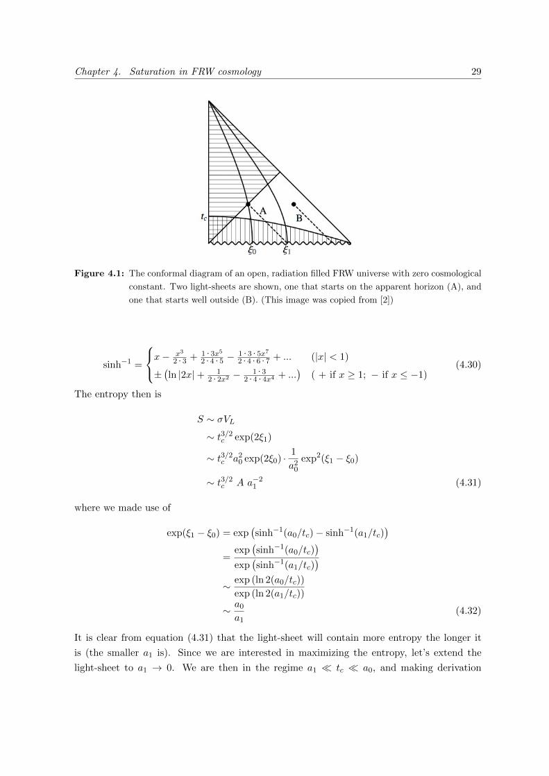
Figure 4.1: The conformal diagram of an open, radiation filled FRW universe with zero cosmological

constant. Two light-sheets are shown, one that starts on the apparent horizon (A), and

one that starts well outside (B). (This image was copied from [2])

sinh!1 =

/0

1x% x3

2 · 3 + 1 · 3x5

2 · 4 · 5 % 1 · 3 · 5x7

2 · 4 · 6 · 7 + ... (|x| < 1)

±'ln |2x|+ 1

2 · 2x2 % 1 · 32 · 4 · 4x4 + ...

(( + if x # 1; % if x $ %1)

(4.30)

The entropy then is

S ! $VL

! t3/2c exp(2*1)

! t3/2c a20 exp(2*0) ·1

a20exp2(*1 % *0)

! t3/2c A a!21 (4.31)

where we made use of

exp(*1 % *0) = exp'sinh!1(a0/tc)% sinh!1(a1/tc)

(

=exp

'sinh!1(a0/tc)

(

exp'sinh!1(a1/tc)

(

! exp (ln 2(a0/tc))

exp (ln 2(a1/tc))

! a0a1

(4.32)

It is clear from equation (4.31) that the light-sheet will contain more entropy the longer it

is (the smaller a1 is). Since we are interested in maximizing the entropy, let’s extend the

light-sheet to a1 ' 0. We are then in the regime a1 , tc , a0, and making derivation

Chapter 4. Saturation in FRW cosmology 30

similar to equations (4.31) and (4.32) we find for the entropy on the light-sheet:

S ! $VL

! t3/2c A

2exp(*1 % *0)

a0

32

! t3/2c A

2exp(ln 2(a0/tc))

a0 exp(a1/tc)

32

! t3/2c A1

t2c

1

(1 + a1/tc)2

! A

t1/2c

41% 2

a1tc

5(4.33)

Extending the light-sheet to the big bang (a1 ' 0 in equation (4.33)) does not add significant

entropy to the light-sheet when we end it at tc ( a1 ' tc in equation (4.31)). Up to factors of

order one, the entropy/area ratio will be

S

A! t!1/2

c (4.34)

Using tc # 1 and A1/4 # 1/t1/2c , it follows that A3/4 , S $ A. The entropy will thus violate

equation (4.2) in this example. Choosing tc ! 1, i.e. a very early curvature domination of

the order of the Planck time, one can saturate the holographic bound. We remark that in

this case, the final edge of the light-sheet will be near the Planck regime.

Pressureless Matter

The same results can be obtained in an open universe filled with pressurless dust, instead of

radiation. The first di!erence will concern the energy density of the pressureless dust, which

is given by8#+

3=

tca3

, (4.35)

which results in the following Friedmann equation,

a2a2 = tca+ a2. (4.36)

We will again choose a sphere well inside the curvature era, tc , a0 , t!, and who’s area

exceeds the apparent horizon, *0 > *AH - 12 ln(

a0tc). This last equation can be deduced by

using AAH = 32% ! a30

tcand AAH ! a20 exp(2*AH). The past outgoing light-sheet is then given

by

*(a) = *0 +

& a0

a

da.tca+ a2

= *0 + 2 sinh!1"%

a0/tc$% E sinh!1

"%a/tc

$, (4.37)

Chapter 4. Saturation in FRW cosmology 31

where we made use of&

dx.ax+ x2

= 2a

& %xad

%xa.

ax%1 + x/a

= 2 sinh!1%x/a. (4.38)

Furthermore, the entropy density of the pressureless dust is of the order of the number density

of the particles,

s ! +

m! tc

ma3. (4.39)

The same argument concerning a1 applies in this case: the dominant contribution will be come

from the curvature dominated era, and hence we will set a1 = tc as before. The comoving

volume contained by the light-sheet will be

VL ! e2&1 !! e2&0 ! e2(&1!&0)

! e2&0exp4(ln

6662%

a0/tc666)

expO(1)

! e2&0a20t2c

(4.40)

We finally find, using A ! a20e2&0 ,

S/A =tcm

VL

A= (mtc)

!1 (4.41)

If we choose the radius large enough, satisfying 1 < mtc < A1/4, the entropy will again exceed

the naive S $ A3/4. For mtc ' 1, the holographic entropy bound will be saturated. The

case mtc , 1 is impossible, since equation (4.39) is only valid if the particles are dilute. This

translates in the requirement that the density of the particles is less than one particle per

Compton wavelength cubed,

&Compt =h

mc

+/m < &!3Compt = m3 ) t!2

c /a3 < m4 (4.42)

If we want last equation to be valid for all a in the considered era a1 $ a $ a0, it follows that

t!1/2c < m (4.43)

The assumption of an entropy density as in equation (4.39) thus allows a saturation of the

holographic bound, but it can never be violated (cfr. FMW).

4.3.2 Positive Cosmological Constant

In the case of an open universe with positive cosmological constant, the apparent horizon will

be

AAH(t) =3

2 (+! + +r)= 4#

4t2ca4

+1

t2!

5!1

(4.44)

Chapter 4. Saturation in FRW cosmology 32

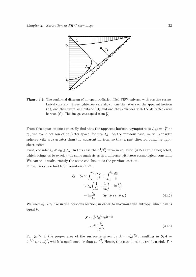
Figure 4.2: The conformal diagram of an open, radiation filled FRW universe with positive cosmo-

logical constant. Three light-sheets are shown, one that starts on the apparent horizon

(A), one that starts well outside (B) and one that coincides with the de Sitter event

horizon (C). This image was copied from [2]

From this equation one can easily find that the apparent horizon asymptotes to AdS = 12"! !

t2!, the event horizon of de Sitter space, for t & t!. As the previous case, we will consider

spheres with area greater than the apparent horizon, so that a past-directed outgoing light-

sheet exists.

First, consider tc , a0 $ t!. In this case the a4/t2! term in equation (4.27) can be neglected,

which brings us to exactly the same analysis as in a universe with zero cosmological constant.

We can thus make exactly the same conclusion as the previous section.

For a0 & t!, we find from equation (4.27),

*1 % *0 !& a0

t!

t!daa2

+

& t!

tc

da

a

! t!

41

t!% 1

a0

5+ ln

t!tc

! lnt!tc

(a0 & t! & tc) (4.45)

We used a1 ! tc like in the previous section, in order to maximize the entropy, which can is

equal to

S ! t3/2c e2&0e&1!&0

! e2&0t2!

t1/2c

(4.46)

For *0 # 1, the proper area of the surface is given by A ! a20e2&0 , resulting in S/A !

t!1/2c (t!/a0)

2, which is much smaller than t!1/2c . Hence, this case does not result useful. For

Chapter 4. Saturation in FRW cosmology 33

*0 , 1, on the other hand, one obtains S/A ! t!1/2c (AdS/A), where we used AdS ! t2!.

Since the surface is assumed bigger than the apparent horizon, and since exp *0 , 1 one finds

AdS $ A , a20. An initial area close to the de Sitter event horizon will result in

S/A ! t!1/2c . (4.47)

A special case will arise when taking a0 ' *, *0 ' 0, A = AdS . The light-sheet will then

correspond to the de Sitter event horizon, which can be seen to saturate the holographic

bound if the curvature era begins very early, tc ' A.

Pressureless Matter

This case can readily be applied to a universe filled with pressureless dust. The Friedmann

equation is

a2a2 = tca+ a2 +a4

t2!. (4.48)

Both the tc , t0 $ t! and the t! , t0 case are completely analogous to the radiation

dominated universe, and hence the same results are obtained.

4.3.3 Negative Cosmological Constant

For a radiation-filled universe with negative cosmological constant, the apparent horizon is

AAH(t) =3

2 (+! + +r)= 4#

4t2ca4

% 1

t2!

5!1

(4.49)

The negative vacuum energy implies that at a time t$ = (tct!), the total energy density will

vanish and then become negative, as follows from

+tot = 0 ) 8#+!3

=8#+r3

) t2ct2! = a4 (4.50)

The apparent horizon becomes infinite for t ' t$, and does not exist at any later times.

Hence, the past-directed outgoing light sheets will only exist for times smaller then t$. We

will therefore require a0 < t$, and since t$ , t!, the last term in equation (4.27) can again be

neglected. The analysis will be identical to the # = 0 case, where the entropy exceeds A3/4,

and approximately saturates the holographic bound for tc ' 1.

However, an additional class of light-sheets can be found who’s entropy exceeds A3/4. The

spheres under consideration will be normal. Consider t$ $ t0 $ tf % t$. During this era,

all spheres are normal since there is no apparent horizon. We will look at the past directed

ingoing light-sheet (the future-directed case is analogous). Suppose we terminate the light-

sheet at the time t$, then it follows from

%* = *0 % *$ !& t0

t!

da

a! ln

t0t$

(4.51)

Chapter 4. Saturation in FRW cosmology 34

Figure 4.3: The conformal diagram of an open, radiation filled FRW universe with negative cosmo-

logical constant. Two light-sheets are shown, one that starts on the apparent horizon

(A), and one that starts well outside (B). This image was copied from [2]

that %* will exceed unity if t0 is at least a few times larger than t$. In this case the comoving

volume can be approximated by VL - Vc(*0), and the entropy on the light sheet S ! e2&0t3/2c .

The initial area is A ! a20e2&0 , hence

S/A ! t3/2c

t20(4.52)

This ratio can be maximized for t0 ' t$, obtaining S/A ! t!1/2c

tct!. Due to tc , t!, this is

a lot smaller than the ratio t!1/2c in the anti-trapped case. The holographic bound cannot

be saturated, however the light-sheets do violate the naive S $ A3/4 if we choose the initial

radius large enough (choosing t3/2c /t20 & A!1/4 ! a!1/20 e!&0/2).

This class of light-sheets can also be found in flat universes with negative cosmological con-

stant. In the flat case, the turnaround time tf/2 (for which a = 0) is given by

0 = t2c %a4

t2!) tf/2 = t$. (4.53)

The apparent horizon will now only diverge at this point in time, and hence for very large

comoving radius, normal spheres will exist only for a very short time around tf/2. Consider

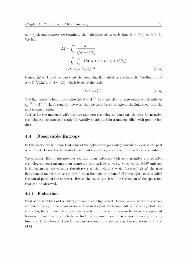
Chapter 4. Saturation in FRW cosmology 35

t0 = tf/2, and suppose we terminate the light-sheet at an early time t1 = t2!/tc , t! < tc.

We find

%* =

& t!

t1

da-t2c % a4/t2!

!& t!

t1

da

tc(for t1 < a < t$ : t

2c > a4/t2!)

! t$/tc = (t!/tc)1/2 (4.54)

Hence, %* , 1, and we can treat the comoving light-sheet as a thin shell. We finally find

S ! t3/2c *20%* and A ! t2$*20 , which leads to the ratio

S/A ! t!1/2! (4.55)

The light-sheet is found to violate the S $ A3/4 for a su"ciently large radius which satisfies

t!1/2! & A!1/4. Let’s remark, however, that we were forced to extend the light-sheet into the

anti-trapped region.

Just as for the universes with positive and zero cosmological constant, the case for negative

cosmological constant can straightforwardly be adapted for a universe filled with pressureless

dust.

4.4 Observable Entropy

In this section we will show that some of the light-sheets previously considered exist in the past

of an event. Hence the light-sheet itself and the entropy contained on it will be observable.

We consider, like in the previous section, open universes with zero, negative and positive

cosmological constant and a curvature era that satisfies tc , t!. Since we the FRW universe

is homogeneous, we consider the observer at the origin, * = 0. Let’s call L(tE) the past

light-cone of an event at tE and * = 0, then the disjoint union of all these light-cones is called

the causal patch of the observer. Hence, the causal patch will be the region of the spacetime

that can be observed.

4.4.1 Finite time

First of all, let’s look at the entropy on one such a light-sheet. Hence, we consider the observer

at finite time tE . The cross-sectional area of its past light-cone will vanish at tE , but also

at the big bang. Thus, there will exist a sphere of maximum area in between, the apparent

horizon. The time t0 at which we find the apparent horizon is a monotonically growing

function of the observer time tE , as can be shown in a similar way like equations (4.5) and

(4.6).

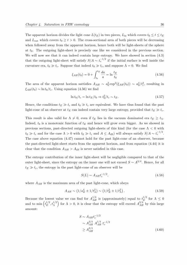
Chapter 4. Saturation in FRW cosmology 36

The apparent horizon divides the light cone L(tE) in two pieces, Lin which covers t0 $ t $ tE

and Lout which covers t0 # t > 0. The cross-sectional area of both pieces will be decreasing

when followed away from the apparent horizon, hence both will be light-sheets of the sphere

at t0. The outgoing light-sheet is precisely one like we considered in the previous section.

We will now see that it can indeed contain large entropy. We have showed in section (4.3)

that the outgoing light-sheet will satisfy S/A ! t!1/2c if the initial surface is well inside the

curvature era, t0 & tc. Suppose that indeed t0 & tc, and suppose # = 0. We find

*AH(t0) = 0 +

& tE

t0

da

a= ln

tEt0

(4.56)

The area of the apparent horizon sattisfies AAH ! a20 exp2(*AH(t0)) ! a40/t

2c , resulting in

*AH(t0) ! ln t0/tc. Using equation (4.56) we find

ln t0/tc = ln tE/t0 ) t20/tc ! tE . (4.57)

Hence, the conditions tE & tc and t0 & tc are equivalent. We have thus found that the past

light-cone of an observer at tE can indeed contain very large entropy, provided that tE & tc.

This result is also valid for # /= 0, even if tE lies in the vacuum dominated era tE # t!.

Indeed, t0 is a monotonic function of tE and hence will grow even bigger. As we showed in

previous sections, past-directed outgoing light-sheets of this kind (for the case # < 0 with

t0 & tc and for the case # > 0 with t0 & tc and A $ AdS) will always satisfy S/A ! t!1/2c .

The case above equation (4.47) cannot hold for the past light-cone of an observer, because

the past-directed light-sheet starts from the apparent horizon, and from equation (4.44) it is

clear that the condition AAH > AdS is never satisfied in this case.

The entropy contribution of the inner light-sheet will be negligible compared to that of the

outer light-sheet, since the entropy on the inner one will not exceed S ! A3/4. Hence, for all

tE & tc, the entropy in the past light-cone of an observer will be

S(L) ! AAHt!1/2c , (4.58)

where AAH is the maximum area of the past light-cone, which obeys

AAH !'1/a4E ± 1/t2!

(!

'1/t2E ± 1/t2!

(. (4.59)

Because the lowest value we can find for A1/4AH is (approximately) equal to t1/2E for # $ 0

and to min"t1/2E , t1/2!

$for # > 0, it is clear that the entropy will exceed A3/4

AH by this large

amount:

S ! AAHt!1/2c

! A3/4AH A1/4

AH t!1/2c

# A3/4AH (4.60)

Chapter 4. Saturation in FRW cosmology 37

4.4.2 The Causal Patch

Now let’s consider the entropy in the whole causal patch, by taking tE ' *. From equations

(4.59) and (4.60) it is clear that, in the # = 0 case, the entropy is unbounded. We will now

look at the two remaining cases # < 0 and # > 0.

Positive Cosmological Constant

In the # > 0 case, the past light-cone becomes the de Sitter event horizon when taking the

limit tE ' *. Its area is decreasing everywhere towards the big bang, hence the whole horizon

is one light-sheet. Moreover, all the observable radiation will pass through this horizon, and

hence the entropy contained on the light-sheet will be the maximum possible observable

entropy, Smax. The same light-sheet was obtained, albeit using another limit, under equation

(4.47). The entropy on it will therefore be equal to

Smax ! AdSt!1/2c ! #!1t!1/2

c (4.61)

For t! & tc we have #!1/4 & t!1/2c and the bound Smax < #!3/4, which holds for a flat

radiation dominated FRW universe, is exceeded. For early curvature domination, the entropy

will be Smax ' #!1.

Negative Cosmological Constant

In the case of a negative cosmological constant, the light-cone of an event at tE ' * will

reach *max = 2*turn, because the evolution is symmetric about the time of maximal expansion

tturn. We can calculate this coordinate,

*turn !& amax

0

da-t2c + a2 + a4/t2!

!& amax

tc

da

a! ln

t!tc

(4.62)

The entropy inside a sphere with comoving radius * is S(*) = $Vc(*), and like before we

will use $ ! t3/2c . The comoving volume for the case tE ' * can be approximated as

Vc ! exp(2*max) ! e4&turn . Hence the entropy in the causal patch will be

Smax ! t4!

t5/2c

! #!2t!5/2c (4.63)

Again, this shows that the observable entropy violates the naive S < |#|!3/4 and that it

approaches Smax ' #!2 in the limit of early curvature domination.

Let’s note that the time t0, where the causal patch intersects the apparent horizon, obeys

tc , t0 , t!. The first inequality originates from the monotonicity of t0(tE), the second

Chapter 4. Saturation in FRW cosmology 38

from t0 ! t$ and t$ , t!. The comoving radius at t0 is

*(t0) = *max %& t0

0

da-t2c + a2 + a4/t2!

! *max %& t0

tc

da

a

! *max % ln t0/tc (4.64)

and hence the area of the apparent horizon will be

AAH ! t20 e2(2&turn!ln t0/tc) ! #!2t!2c (4.65)

We therefore find Smax/AAH ! t!1/2c , which is consistent with what we found previously,

considering Smax ! S(Lout).

4.5 Gravitational Collapse

In the previous sections we considered several cosmological examples. However, the initial

conditions of all those consisted of many causally disconnected regions near to the big bang.

It is hence impossible to find a future light-cone of an observer containing all those regions.

Therefore, in this section we will describe some examples that do exist in such a future

light-cone, and can hence be created by an experimentalist starting in flat space.

4.5.1 Collapsing Ball of Dust

Consider again the situation of section 4.3.1, for the case of pressureless matter. In the far

future, the matter density becomes increasingly dilute and the open FRW space becomes

increasingly flat, approaching flat Minkowski. Imagine that now we reverse the time for that

solution, then we start from a flat Minkowski. The observer in the previous section, that had

a past light-cone containing the saturating light-sheet, will now become an observer with a

future directed light-cone containing a saturating light-sheet. This is exactly the situation we

were looking for.

Consider a pressureless dust ball, in fact the time-reversed cosmology, with maximal comoving

radius *max. Outside we assume vacuum. The metric outside will be that of the Schwartzschild

black hole metric, as dictated by the Birkho! theorem,

ds2 = %41% 2M

r

5d,2 +

41% 2M

r

5!1

dr2 + r2d$2 (4.66)

We now have to find the relation between the Schwarzschild variables (M, r, ,) the cosmolo-

gical variables (tc, *, t), describing the space outside and inside the dust ball respectively. In

order to do so, consider a geodesic in the cosmology at fixed *max, on the boundary between

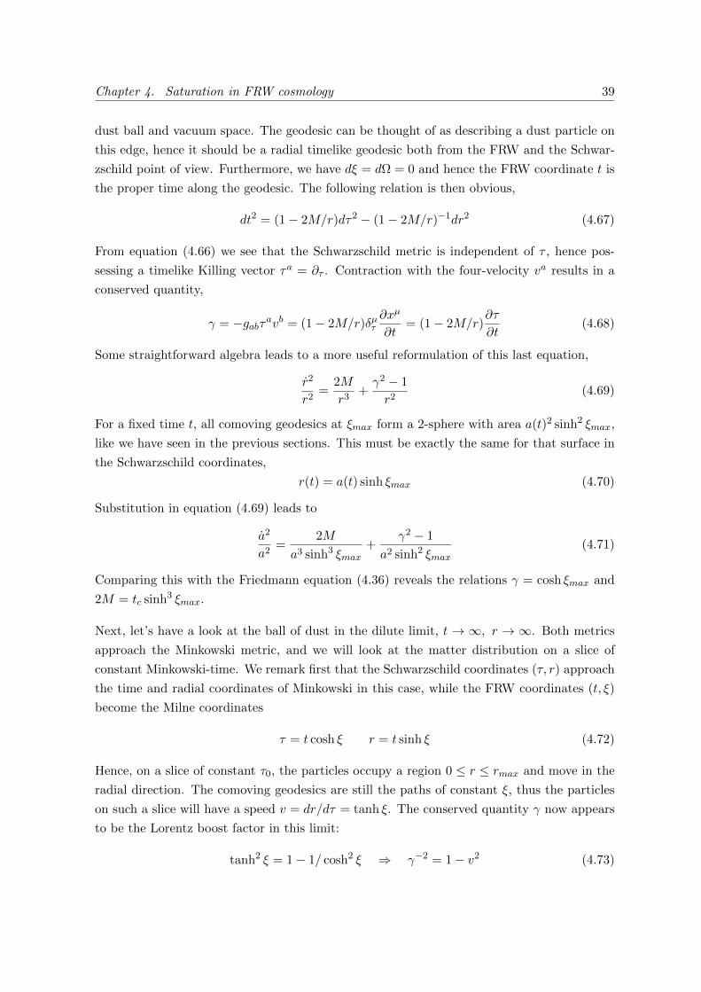
Chapter 4. Saturation in FRW cosmology 39

dust ball and vacuum space. The geodesic can be thought of as describing a dust particle on

this edge, hence it should be a radial timelike geodesic both from the FRW and the Schwar-

zschild point of view. Furthermore, we have d* = d$ = 0 and hence the FRW coordinate t is

the proper time along the geodesic. The following relation is then obvious,

dt2 = (1% 2M/r)d,2 % (1% 2M/r)!1dr2 (4.67)

From equation (4.66) we see that the Schwarzschild metric is independent of , , hence pos-

sessing a timelike Killing vector ,a = )' . Contraction with the four-velocity va results in a

conserved quantity,

- = %gab,avb = (1% 2M/r).µ'

)xµ

)t= (1% 2M/r)

),

)t(4.68)

Some straightforward algebra leads to a more useful reformulation of this last equation,

r2

r2=

2M

r3+

-2 % 1

r2(4.69)

For a fixed time t, all comoving geodesics at *max form a 2-sphere with area a(t)2 sinh2 *max,

like we have seen in the previous sections. This must be exactly the same for that surface in

the Schwarzschild coordinates,

r(t) = a(t) sinh *max (4.70)

Substitution in equation (4.69) leads to

a2

a2=

2M

a3 sinh3 *max+

-2 % 1

a2 sinh2 *max(4.71)

Comparing this with the Friedmann equation (4.36) reveals the relations - = cosh *max and

2M = tc sinh3 *max.

Next, let’s have a look at the ball of dust in the dilute limit, t ' *, r ' *. Both metrics

approach the Minkowski metric, and we will look at the matter distribution on a slice of

constant Minkowski-time. We remark first that the Schwarzschild coordinates (,, r) approach

the time and radial coordinates of Minkowski in this case, while the FRW coordinates (t, *)

become the Milne coordinates

, = t cosh * r = t sinh * (4.72)

Hence, on a slice of constant ,0, the particles occupy a region 0 $ r $ rmax and move in the

radial direction. The comoving geodesics are still the paths of constant *, thus the particles

on such a slice will have a speed v = dr/d, = tanh *. The conserved quantity - now appears

to be the Lorentz boost factor in this limit:

tanh2 * = 1% 1/ cosh2 * ) -!2 = 1% v2 (4.73)

Chapter 4. Saturation in FRW cosmology 40

The velocity distribution is now also clear, with the help of equation (4.72) one finds v(r) =

r/,0.

The energy-momentum tensor can now easily be written in Minkowski-space coordinates,

using a(t) = t for the dilute limit,

Tab = +dt2 =3tc8#

dt2

t3=

3tc8#

(,d, % rdr)2

(,2 % r2)5/2(4.74)

The energy density is then the coe"cient of d,2, and the number density can be found by

dividing this by the particle energy -m,

n(r) =1

m-

3tc8#

,20(,20 % r2)5/2

=3tc8#

,0(,20 % r2)2

(4.75)

The total number of particles is

N = 4#

& rmas

0

43tc8#m

,0(,20 % r2)2

5r2dr

=

& &max

0

tanh2 *

(1% tanh2 *)2d tanh *

=3tc2m

& &max

0sinh2 *d*

=3tc8#m

Vc(*max) (4.76)

where we made use of tanh * = r/,0 = v and '0.'20!r2

= 1"1!v2

.

The question now is how to create this situation in Minkowski space. We will thus continue

using the Minkowski coordinates to show that it is possible to find a light-sheet exceeding

S $ A3/4. In order to do so we introduce a parameter /,

S = /A3/4, (4.77)

and show that we can find / > O(1).

Consider a large number of particles N , arranged in a sphere of radius rmax and each with a

mass m. Furthermore, the initial velocities will be chosen in a way that they all converge in

one single point, v(r) + r. These velocities will be near to the speed of light, and it will be

convenient to use the Lorentz boost factor instead of the speed, -(r) = (1% v(r)2)!1/2. Let’s

call the boost factor for the most energetic particles -max = -(rmax). Finally we also require

the number density to be in accordance to equation (4.75), hence n(r) + -(r)4. If we suppose

that -max & 1, equation (4.73) implies that, -max = cosh *max ! sinh *max ! exp(*max)/2.

From equation (4.76) we find

tc =8#Nm

3Vc(*max)! Nm

-2max(4.78)

Chapter 4. Saturation in FRW cosmology 41

Hence, for light-sheets that extend to this point in (FRW) time, the entropy will be, as

calculated in section 4.3.1,

S ! (mtc)!1 A ! -2max

Nm2A (4.79)

Comparison with equation (4.77) learns

/ ! -3/2max

N3/4m3/2S1/4 (4.80)

Fixing -max, N and m, the entropy is the only part that will be variable depending on which

light-sheet we choose. Obviously we want to look at the light-sheet that will contain the most

entropy, which can be maximally S ! N . There is a light-sheet that will indeed have such

an entropy, namely the one that starts on the apparent horizon and reaches * = *max at the

time t = tc. We then have

/ !4-3max

Nm3

51/2

. (4.81)

From section 4.3.1, we know that m > t!1/2c is needed for the validity of the entropy counting

we used. Saturating this will lead to the maximum possible entropy-area ratio. Indeed, it

then follows that -2max ! Nm3, which finally gives

/ ! (Nm3)1/4 ! -1/2max (4.82)

And since we assumed -max & 1, we find indeed / > O(1).

4.6 Saturation Within a Causal Diamond

The previous examples convinced us that the bound S $ A3/4 is not generally valid. This

doesn’t mean that it cannot be valid under certain conditions. All our examples in the

previous sections do not lie within a causal diamond, hence we will investigate if the naive

bound can be violated for the latter situation. A causal diamond of a worldline is the region

of space-time which can both receive signals from and send signals to that worldline. In other

words, we will investigate the entropy of systems that can be both set up and observed by

the same person.

4.6.1 Shell of Dust in AdS

The metric of the empty AdS space can be written in the following way,

ds2 = %dt2 + a2(,)(d02 + sinh2 0d$22), (4.83)

with a(t) = t! sin(t/t!). We will now add a spherically symmetric shell of dust. The density

of the matter should be low, in order to be able to use the vacuum metric nonetheless. We

assume the dust at rest, and this will remain so since the worldlines with constant spatial

Chapter 4. Saturation in FRW cosmology 42

coordinates are geodesics. Let 0max and 0min be the comoving radius of the boundaries of

the shell.

Let’s consider the condition on the density of the dust. We require it to be only a small

perturbation at the turnaround time t = t!#/2, which implies that the density should be

negligible compared to the vacuum energy,

+m , 1

t!(4.84)

At the turnaround time, the scale factor is maximal. This means that the dust will follow

converging geodesics, and the probe approximation will not be valid any longer. The metric

in the dust shell will only be approximated by (4.83) as long as the matter density obeys

(4.84).

Let’s now calculate the future directed ingoing light-sheet. The past directed ingoing light-

sheet can be calculated in the same way, since the space-time is symmetric about the turn-

around time. Hence, if we find that they reach the origin, the matter is contained in the

causal diamond of the observer in the origin. The radial light rays are given by

d0 =dt

a(t)(4.85)

which can be rewritten using a2 = 1% a2

t2!,

d0 =da

a-1% a2/t2!

(4.86)

Integrating equation (4.86) leads to

%0 = cosh!1

4t!a

5(4.87)

From this equation, it follows that the light will travel one comoving radius %0 = 1 in the

time that the scale factor a decreases a few times smaller than t!, and the density increases as

+m ! a!3. Hence, if we choose the shell extend over one comoving radius, and if we suppose

the initial matter density to be a lot less than the vacuum energy, our probe approximation

remains valid until the light-sheet escapes from the shell. The light-sheet will now certainly

reach the origin: the metric inside the shell is the vacuum AdS metric, and the dust particles

at the inner boundary of the shell will follow a timelike geodesic. The light rays, following

null geodesics, are thus certain to reach the origin before the metric would be a!ected by the

collapsing matter.

We will now calculate S/A for the previous light-sheet. Suppose the matter to be nearly

relativistic, then the relation between entropy density and matter energy density is

s ! +3/4m (4.88)

Chapter 4. Saturation in FRW cosmology 43

The entropy will then be bounded below by the entropy on the spatial slice at the turnaround

time, which has maximal expansion coe"cient. The entropy on this spatial slice is, using

%0 = 1 and a = t! at the turnaround time,

S = sV = +3/4m At! (4.89)

Finally, to remain in the probe approximation, we have +m < +!. The entropy-area ratio will

therefore be

S/A $ t!3/2! t! $ t!1/2

! (4.90)

For a large comoving radius *, one can obtain A & #!1 and therefore a light-sheet with

S & A3/4 within a causal diamond.

4.6.2 Slow Feeding of a Black Hole

Let’s consider a black hole of radius R. Imagine we send massless quanta into this black hole,

one at the time. The wavelength of each quantum is &, and the energy is &!1. Hence the

black hole will have doubled his energy and radius after R& quanta have been absorbed. The

area of the black hole horizon will now be 4#(2R)2. This surface possesses a past-directed

ingoing light-sheet which coincides with that part of the event horizon that absorbed the R&

quanta. The light-sheet will therefore have an entropy of order R&, the number of quanta

that crosses the light sheet one by one. We therefore find the ratio

S

A! &

R(4.91)

We first remark that the covariant bound will not be violated, since the quanta with wavelengths

& & R will not be absorbed by the black hole. In the limit & ' R, we see that the bound

can be saturated, and if we choose quanta with & & R1/2, the bound S $ A3/4 is violated.

For an observer at a fixed radius outside the black hole, the light-sheet discussed in this

example is part of the boundary of this observer’s causal diamond. Hence, this example

shows that a light-sheet with S & A3/4 can exist within a causal diamond.

Chapter 5

Bianchi Type I model

In the previous chapter, several examples were found that violate the naive bound S < A3/4,

and some that even saturate the CEB. These examples di!er from previous work in the fact

that they consider cosmologies with a physical matter content and observable light-sheets. In

this chapter, we will proceed in an analogous way, but our model under consideration will

be anisotropic. Our goal will be to find more examples that violate S < A3/4, considering

a dust-filled universe. In the next chapter we will repeat this exercise for an inhomogeneous

model.

Consider the Bianchi type I universe model, which has the following metric:

ds2 = % dt2 +X2(t) dx2 + Y 2(t) dy2 + Z2(t) dz2 (5.1)

This model describes the simplest anisotropic generalisation of the flat FRW models. Spa-

tially, these models are homogeneous. The average expansion scale factor is given by

S(t) = (XY Z)1/3 (5.2)

The generalized Friedmann equation is[9]

3S2

S2=

&2

S6+

M

S3((5.3)

where - is determined by the perfect fluid equation of state between the fluid’s pressure p

and density µ,

p = (- % 1)µ, - = 0 (5.4)

and M is given by

µ =M

S3(, M = 0 (5.5)

A tetrad can be found by

ei) = *!1) .i) (5.6)

44

Chapter 5. Bianchi Type I model 45

where *0 = 1, *1 = X(t), *2 = Y (t), *3 = Z(t). The tetrad should obey[9]

[e), e0] =

)S

S.*) + $ *

)

*e* (5.7)

where $*) is the shear tensor, which describes the rate of distortion of the matter flow. This

tensor will satisfy[9]

$)* =&)*

S3, $2 =

&2

S6, &2 =

1

2&)*$

)* (5.8)

with &*) a constant tensor. From equation (5.7) we find

0% e0e) =S

Se) + $ *

) e*

) *)*2)

)

)*)=

*)*)

e) =S

Se) + $ *

) e*

) *)*)

. *) =

S

S. *) + $ *

) (5.9)

Hence, the non-vanishing components of the shear tensor are

$11 =X

X% S

S, $22 =

Y

Y% S

S, $33 =

Z

Z% S

S(5.10)

We will now calculateX(t), and the other scale factors can be calculated analogously. Suppose

the function X(t) is of the form X(t) = S(t) f(t), with f a function to be determined. Writing

&11 = &1, equations (5.8) and (5.10) then imply

f

f=

&1

S3) f = exp

4&1

&dt

S3

5(5.11)

Hence, the individual length scales are given by

X(t) = S(t) exp(&1W (t)), Y (t) = S(t) exp(&2W (t)), Z(t) = S(t) exp(&3W (t)) (5.12)

with W (t) =.

dtS3(t) and

&1 + &2 + &3 = 0, &21 + &2

2 + &23 = 2&2 (5.13)

From equation (5.12) we can see that the case in which & = 0 would correspond to the

isotropic case. The solution to equations (5.13) is given by

&) = (2&/.3) sin/), /1 = /, /2 = /+ 2#/3, /3 = /+ 4#/3 (5.14)

with / a constant.

Chapter 5. Bianchi Type I model 46

In the case of dust, we have - = 1, and it follows from the Friedmann equation (5.3) that

1

3

S3

S3=

S

S=

&2

S6+

M

S3(

) d(S3)%&2/M + S3

=.3Mdt

)%&2/M + S3 =

.3M

2t+ C

) S(t) = (3

4Mt2 +

.3&t)1/3 (5.15)

were we determined the integration constant C =%

&2/M such that the average expansion

factor S is zero when t = 0. From W =.dt/S3 it is then easy to find

W (t) =1.3&

ln

)t

34Mt+

.3&

*, (5.16)

which finally leads to

X(t) = S(t)

4t2

S(t)3

5 23 sin)1

, Y (t) = S(t)

4t2

S(t)3

5 23 sin)2

, Z(t) = S(t)

4t2

S(t)3

5 23 sin)3

(5.17)

We will consider the case in which two coordinate directions have the same length scale. From

equation (5.17) we see that such cases occur when / = #/2 or / = #/6. We will use the

former, but the latter is analogous. Hence, using / = #/2 we get

X(t) =t4/3

S(t), Y (t) = Z(t) = S2(t)t!2/3 =

t2

X2(t)(5.18)

For simplicity, let’s rewrite some of the previous equations in our specific case of dust-filled

Bianchi type I cosmology. The metric is

ds2 = %dt2 +X2(t)dx2 + Y 2(t)(dy2 + dz2) (5.19)

with X(t) and Y (t) given by (5.18). The average scale factor is

S3(t) =.3&t

4t

tM+ 1

5(5.20)

where

tM =4.3

&

M(5.21)

We will now consider a surface around the origin in the (yz)-plane: let’s choose a disk of

proper area

A = 4#r2Y 2(t0) (5.22)

where r2 = y2 + z2.

Chapter 5. Bianchi Type I model 47

5.1 Case 1

Suppose we have

1 , t0 , tM (5.23)

to leading order in t, we find

S(t) !".

3&$1/3

t1/3

X(t) !".

3&$!1/3

t

Y (t) !".

3&$2/3

4t

tM+ 1

5(5.24)

The light-sheet will consist of light-rays normal to this surface. From (5.24) we see that in

this regime, t/tM , 1, the scale factor Y (t) is approximately constant. Parallel light-rays

emanating from the surface will therefore remain parallel, and the expansion of the light-

sheet will be vanishing. Consider for example a past directed light-sheet in the direction of

increasing x,

1

X(t)dt = dx

)".

3&$1/3 dt

t= dx

)".

3&$1/3

ln

4t0t1

5= x1 % x0 (5.25)

with t0 > t1 since it is past-directed.

The comoving volume of the light-sheet is

Vc ! r2%x

! r2".

3&$1/3

ln

4t0t1

5

! r2".

3&$1/3

ln t0 (5.26)

where in the last step we assumed the light-sheet to continue until 1 $ t1 , t0. Assuming

the comoving entropy density for dust to be equal to the number density, $ = M/m, with

M the total mass per comoving unit volume and m the mass of one dust particle, the total

entropy on the light-sheet will be

S ! $VC ! r2".

3&$1/3

ln t0M

m(5.27)

From equation (5.22), the area of our initial surface is

A ! r2".

3&$4/3

(5.28)

Chapter 5. Bianchi Type I model 48

Hence, we find an entropy/area ratio equal to

S

A! 1

m

ln t0tM

(5.29)

For large enough comoving coordinates y and z, the bound S $ A3/4 can be violated. This

can be achieved choosing

r1/2 & &2/3

$ ln t0, (5.30)

The covariant bound will still hold, since the formula for the entropy density to be equal

to the number density is only valid when the number density is less than one particle per

Compton wavelength cubed, resulting in

m4 > µ ! M

S3! (ttM )!1 (5.31)

This should be hold in the interval 1 < t < tM , hence m > t!1/4M . The largest entropy/area

ratio for this case will then approximately be S/A ! tM/ ln(tM ) < 1.

5.2 Case 2

Suppose 1 < tM , t0. In this regime, the scale factors can be approximated by

S(t) !4

&

tM

51/3

t2/3

X(t) !4

&

tM

5!1/3

t2/3

Y (t) !4

&

tM

52/3

t2/3 (5.32)

The light-rays start parallel and will diverge due to the expansion of the universe orthogonal

to the x-dimension. Hence light-sheets should be past-directed, in order to have a negat-

ive expansion. The equation of a past directed light-sheet, in the direction of decreasing x

coordinate, is

dt

X(t)= dx

)3

4tM.3&

5!1/3

(t1/30 % t1/31 ) = x0 % x1 (5.33)

The comoving volume of the light-sheet is

Vc ! %x r2 ! r24tM&

5!1/3

(t1/30 % t1/31 ) (5.34)

Chapter 5. Bianchi Type I model 49

We can now calculate the entropy on the light-sheet, using $ = M/m,

S ! $Vc ! r2$(&/tM )1/3t1/30 , (5.35)

assuming the light-sheet extending until tM , t1 , t0. The area of the initial surface is

equal to A ! r2(&/tM )4/3t4/30 , henceS

A! 1

m t0(5.36)

Choosing r & (Mt0)4/3

!2 , the naive bound S $ A3/4 will be violated. The same argument as

the one we mentioned in the end of section (5.1) can be used to show the covariant bound

holds, and since t0 & 1, the light-sheet will not be able to saturate the CEB.

A major remark is that the stronger bound (3.9) should be considered in both previous cases.

In the first case, the derivation should still hold if were able to neglect the entropy contribution

of the part of the light-sheet that continues until t = 0. However our approximation is not

suitable to calculate such a light-sheet. In the case we apply the stronger bound (3.9), than

we should keep the t/tM term in equation (5.24), resulting in A(t0)%A(t1) ! r2 (&)4/3 t0/tM .

This leads to the fact that the CEB only holds if

t0ln t0

> t1/4M (5.37)

The entropy bound would be violated otherwise, and we could argue that in (a part of) this

regime, t < tM , a quantum gravitational description is still needed. From equation (5.24) we

can indeed see that if t , tM , at least for the y and z dimensions the situation is not much

di!erent then for the big bang t = 0. Provided that, for large enough t0 such that equation

(5.37) is satisfied as well as the other requirements of section (5.1), the above derivation

would still hold. Then this case shows a new way of violating S < A3/4 since it would be

only possible for this anisotropic model. Indeed, the time tM and hence the regime under

consideration does not exist in isotropic models.

In the second case, the derivation presented is a good approximation even for the stronger

bound (3.9) since A(t0)%A(t1) ! A(t0). From equation (5.17), we see that at late times the

universe isotropizes. Hence this case should not be restricted to only anisotropic models.

Chapter 6

Lemaitre-Tolman-Bondi model

Consider the case of a spherically symmetric inhomogeneous model of the universe. The

metric of such a model describing a dust-filled universe in matter-comoving coordinates is

ds2 = %dt2 +(Y #(t, r))2

1 + 2E(r)dr2 + Y 2(t, r)d$2 (6.1)

This is the Lemaitre-Tolman-Bondi metric, with d$2 = d'2 + sin2 ' d12 and Y (t, r) obeying

a generalized Friedmann equation,

Y (t, r) = ±

72M(r)

Y (r, t)+ 2E(r) (6.2)

We use the convention that a dot represents the partial time derivative )/)t, while a prime

stands for the partial radial derivative )/)r. The energy density is determined by

4# µ(t, r) =M #(r)

Y 2(t, r)Y #(t, r)(6.3)

Equation (6.2) has the solution [9]

Y (t, r) =M(r)

E(r) 10(t, r), *(t, r) =(E(r))3/2 (t% tB(r))

M(r)(6.4)

with

E(r) =

/8880

8881

2E(r)

1

%2E(r)

10 =

/8880

8881

cosh ! % 1

(1/2)!2

1% cos !

* =

/8880

8881

sinh ! % !

(1/6)!3

! % sin !

when =

/8880

8881

E > 0

E = 0

E < 0

(6.5)

with ! = !(t, r) a parameter. The model is characterized by the three arbitrary functions

M(r), E(r), tB(r). The function tB(r) is the local time at which Y = 0, or in other words the

time of the local big bang.

50

Chapter 6. Lemaitre-Tolman-Bondi model 51

6.1 Parabolic solution

We will first consider the E = 0 solution of the LTB-model, which is called the parabolic

solution. From equations (6.4) and (6.5) we find

M(r) =6(t% tB)

!3

Y (r, t) = M(r)!2

2(6.6)

Eliminating the parameter ! in the previous equations results in

Y (t, r) =

49

2M(t% tB)

2

51/3

(6.7)

Suppose we choose the function tB(r) to be rapidly converging to a constant C for comoving

radius bigger than rc. For example, the function

tB(r) = % 1

10x+ 1+ 1 (6.8)

will be approximately equal to one for r > 1. Di!erentiating equation (6.7) with respect to r

yields

Y # =Y

3MM # % 2

3

Y

t% tBt#B (6.9)

As one can easily see, the area of a sphere centered around the origin is equal to

A = 4#Y 2 (6.10)

Assuming this sphere well outside rc and at a time t0 & C, we can write

A ! M2/3(r0),4/30 (6.11)

where , = t%C. Let’s now suppose rc is su"ciently small, such that M(rc) << M(r0). The

volume of a sphere from tc to t0 is then

V ! 4#

& r0

rc

Y 2Y #dr

! 4

3#

& M0

Mc

Y 3

MdM

! 4

3#9

2,20 (M0 %Mc)

! ,20M0 (6.12)

where we used t#B ! 0. Combining equation (6.9) without the last term, which should be a

good approximation for the region r > rc, with equation (6.3) leads to

4

3#Y 3µ ! M (6.13)

Chapter 6. Lemaitre-Tolman-Bondi model 52

which shows that M(r) can be approximately interpreted as the total mass within a sphere

of radius r.

Radial light rays in the region r > rc will obey

) dt = Y #dr

) dt =YM #

3Mdr

) dt + M!2/3,2/3dM

) ,1/3 + M1/3 (6.14)

Let’s choose the initial sphere bigger than the particle horizon, M0 & ,0. The generating

light-rays for a past, ingoing light-sheet will then obey

,1/30 % ,1/31 + M1/30 %M1/3

1 (6.15)

where we neglected order one factors. Assuming that the light-sheet extends su"ciently into

the past to obtain ,1 , ,0 while staying well outside the sphere of radius rc, we find

M1 ! M0

41% (

,0M0

)1/353

) M1 ! M0 % 3,1/30 M1/30 (6.16)

The entropy density is approximated by the number density of the dust particles. The total

entropy on the light-sheet we constructed above, will then be

S =M0 %M1

m(6.17)

with m the mass of a single dust particle. Combining equations (6.16) and (6.17), we find

S ! t1/30 M2/30

m(6.18)

Dividing the entropy by the area of the surface (6.11), finally leads to

S

A! 1

mt0(6.19)

The covariant bound will indeed hold: the formula for the entropy density to be equal to the

number density is only valid when the number density is less than one particle per Compton

wavelength cubed, resulting in

m4 > µ ! M/Y 3 ! t!2

) m > t!1/2 (6.20)

Chapter 6. Lemaitre-Tolman-Bondi model 53

This should hold for the whole time interval 1 < t1 < t < t0, hence m > t!1/21 & t!1/2

0 and

therefore mt0 > 1. Secondly, by choosing a large enough radius, the naive bound S < A3/4

will be violated. Indeed,

S ! M1/60

mt2/30

A3/4

) S & A3/4 if we choose M0 & m6t40 (6.21)

One way to interpret this result is to remark that, in the regime r > rc which we considered,

the spacetime behaves as a flat FRW universe. Since our case is very similar to that of

truncated light-sheets, our result is somehow expected to violate S < A3/4.

6.2 Hyperbolic solution

A second family of solutions of the LTB equations (6.4) and (6.5), with positive E(r), is called

hyperbolic. In this and the next section we will consider a simultaneous big bang time for all

values of comoving radius r, tB = constant = 0.The solution we will consider is

Y (r, t) = B a(t) exp[R(r +1

r)]

M(r) = C exp[3R(r +1

r)]

E(r) = D exp[2R(r +1

r)] (6.22)

where B,C,D and R are constants, which we will choose positive in this section. This solution

is indeed consistent with equations (6.4) and (6.5), if we set

sinh ! % ! = t, ( cosh ! % 1)! = 1, ! = a!1(t) (6.23)

The function a(t) can be determined by substituting our solution into the Friedmann equation

(6.2),

da-CBa +D

=

.2

Bdt (6.24)

We will assume a(t) to be positive for all t > 0, hence Y (r, t) will be a positive function. Let

us substitute a(t) = ,2(t) and C/(BD) = F in equation (6.24), which results in

&,2d,.F + ,2

=

& %D/2

Bdt (6.25)

which results in

1

2,%F + ,2 +

F

2ln

4F

, +.F + ,2

5=

%D/2

Bt (6.26)

Chapter 6. Lemaitre-Tolman-Bondi model 54

One initial condition we can require is that Y (r, t) vanishes on the big bang time t = 0, which

leads to , = 0 and F = 1. The second term in the left hand side of equation (6.27) will be

negligible, hence the function a(t) can be approximated very well by

a+ a2 ! 2D

B2t2 (6.27)

6.2.1 Anti-Trapped Spheres

We will first investigate the case of a sphere bigger then the apparent horizon. For simplicity,

we will set the all the constants B,C,D and R equal to 1. To avoid the need for a quantum

gravitational description, we will assume t & 1, hence using equation (6.27) we can make

the following approximation: a ! t(.2). Analogous to our derivation in section (4.3), the

apparent horizon is determined bya

a= ± f

f(6.28)

with f = exp(r + 1r ). This leads to

(1% 1/r2)dr = dt/t ) ln t = r + 1/r (6.29)

We see that, for every t > e2 ! 7, 4, there are two apparent horizons: one for rAH,1 > 1 and

one for rAH,2 = 1rAH,1

< 1, hence resulting in two anti-trapped regions (i.e. r > rAH,1 and

r < rAH,2). For smaller times, all spheres are anti-trapped. However, let’s remark that this

apparent horizon is a bad approximation for these smaller times: equation (6.29) does not

specify a relation between time and comoving radius for light rays, and since we made use of

a ! t which is only valid for t & 1. The particle horizon is given by

dt ! t(1% 1

r2)dr ) ln t ! r +

1

r(6.30)

where we used the approximation

exp[R(r + 1r )](1%

1r2 )-

1 + 2 exp[2R(r + 1r )]

!(1% 1

r2 ).2

(6.31)

The apparent horizon and the particle horizon are thus equal, at least in our approximation

for large times.

Consider now a sphere at radius r0 & ln t0 & 1, well outside the biggest apparent horizon.

Analogous to the previous chapter, we will investigate the past outgoing light-sheet. The

light-rays generating this light-sheet obey:

ln(t0/t1) = r1 % r0 (6.32)

Chapter 6. Lemaitre-Tolman-Bondi model 55

Suppose t0 su"ciently large, and imagine we end the light-sheet at an early time, such that

t0 & t1 > 1, then we have r1 & r0 > 1. The comoving volume of a sphere is Vc = V/S3

where S = Y ""1+2E

. Using the approximation (6.31), we get

Vc = 4#

.Y 2 Y "

"1+2E

S3

) Vc !exp(2r + 2/r)

(1% 1/r2)3(6.33)

Using this result, the comoving volume of a the light-sheet becomes Vc ! Vc(r1) % Vc(r0) !Vc(r1) ! exp(2r1). The entropy on the light-sheet is

S ! $ exp(2r1) ! $ exp(2r0)t20t21

(6.34)

where we used equation (6.32). The area of the initial surface is A ! a20 exp(2r0) ! t20 exp(2r0),

which leads us toS

A=

$

t21(6.35)

If the we maximize the comoving entropy density $ ' 1 and the light-sheet t1 ' 1, we see

that the covariant entropy bound can be saturated, but not violated. A remark is that in our

derivation of equation (6.35) we neglected the contribution to the entropy for times near the

big bang. One way to interpret this result, is by remarking that in the limit r > 1, t > 1,

the model is very close to an open FRW universe with zero cosmological constant. Indeed, in

this limit we have Y ! a exp(r) and the metric can be approximated as

ds2 = %dt2 + a24

d(exp r)2

1 + 2 exp(2r)+ exp(2r)d$2

5(6.36)

Let’s now investigate the light-sheets for spheres smaller than the inner apparent horizon.

Let’s assume we will only look at the region of spacetime with 1/r >> 1, then the metric can

be approximated by

ds2 = %dt2 +a2 exp(2/r)

r4(1 + exp(1 + 2/r))dr2 + a2 exp(2/r)d$2 (6.37)

After substituting 1/r = *, we will again find the metric of an open FRW universe with zero

cosmological constant. Therefore, an analysis analogous to the one for the outer apparent

horizon can be repeated in this regime, and will result in a similar conclusion. The solution

under consideration can hence be regarded as a union of two flat FRW spacetimes.

6.2.2 Truncated Light-Sheets

Because the particle horizon and the apparent horizon are approximately equal, the same

spheres we considered in the previous section will have truncated past directed ingoing light-

sheets. Consider now a sphere at radius r0 & ln t0 & 1, well outside the particle horizon.

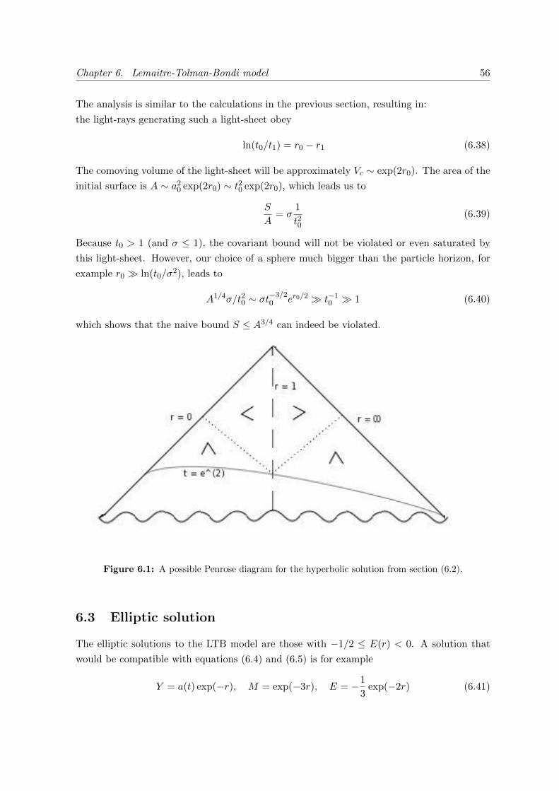
Chapter 6. Lemaitre-Tolman-Bondi model 56

The analysis is similar to the calculations in the previous section, resulting in:

the light-rays generating such a light-sheet obey

ln(t0/t1) = r0 % r1 (6.38)

The comoving volume of the light-sheet will be approximately Vc ! exp(2r0). The area of the

initial surface is A ! a20 exp(2r0) ! t20 exp(2r0), which leads us to

S

A= $

1

t20(6.39)

Because t0 > 1 (and $ $ 1), the covariant bound will not be violated or even saturated by

this light-sheet. However, our choice of a sphere much bigger than the particle horizon, for

example r0 & ln(t0/$2), leads to

A1/4$/t20 ! $t!3/20 er0/2 & t!1

0 & 1 (6.40)

which shows that the naive bound S $ A3/4 can indeed be violated.

Figure 6.1: A possible Penrose diagram for the hyperbolic solution from section (6.2).

6.3 Elliptic solution

The elliptic solutions to the LTB model are those with %1/2 $ E(r) < 0. A solution that

would be compatible with equations (6.4) and (6.5) is for example

Y = a(t) exp(%r), M = exp(%3r), E = %1

3exp(%2r) (6.41)

Chapter 6. Lemaitre-Tolman-Bondi model 57

The Friedmann equation for this solution is

a =

92

a% 2/3 (6.42)

which leads to

da%3/a% 1

=%2/3dt

).3, % 1

,+ 3arctan

'.3, % 1

(= %

%2/3t

) 3 arctan'.

3, % 1(! %

%2/3t (6.43)

where we substituted a = ,!1 in the first line and used t > 1 to make the approximation in

the third line. This results in

a ! cos2(Ct) (6.44)

with C an order one constant. Using the approximation

Y #.1 + 2E

! %a exp(%r) (6.45)

we find that radial light rays obey

tan(t) ! exp(%r) (6.46)

From equation (6.44) we see that the function a(t) becomes zero in at periodic times. However,

for very small a(t) we approach the quantum gravitational regime, and hence the amount of

time the generating light-rays can travel is small. Indeed, the maximum for a(t) = cos2(t) lies

on t = 0+n#, but tan(t) varies slowly around this value. This implies that the light rays travel

only a small comoving distance in the time range allowed for a non-quantum gravitational

description, justifying the approximation Vc ! %(r)Ac ! %(r)A0/(a20 exp(%2r0). Hence we

findS

A! %(r)

e2r0

a20(6.47)

Even though%(r) is small, for large enough r0 we see that the covariant bound can be violated.

However, this violation is due to the fact that Y (r, t) and Y #/.1 + 2E almost vanish even

for large enough r, while a(t) never becomes bigger than one. Hence this spacetime is very

contracted and the quantum gravitational e!ects are expected to be important, proving the

previous calculations incorrect.

This is a general problem for solutions of the form Y = a(t)R(r). Indeed, %1/2 $ E(r) !R2(r) < 0 requires R2(r) not to exceed a certain lower and upper boundary, hence the same

can be said for R(r). The Friedmann equation, in this case, will always result in a ! cos2(f(t))

Chapter 6. Lemaitre-Tolman-Bondi model 58

if we suppose t > 1, but even if we don’t use this approximation a will stay remain bounded,

which is clear from the Friedmann equation (6.42) itself. The limitations on R(r) imply that it

should be periodic or converging to a constant for r ' *. The periodic solution R(r) = sin(r)

gives the closed FRW universe. Indeed, setting E = % sin2(r)/2 results in Y #/.1 + 2E = 1.

The metric becomes

ds2 = %dt2 + a2(t)'dr2 + sin2(r)d$

((6.48)

If the R(r) converges to a constant, on the other hand, for large r the spacetime converges

to one constant surface. Indeed, consider a spherical surface at a time t0 such that a0 > 0.

This surface has area A = 4#a20R2. However, for large r, the area of all such surfaces is

approximately equal since R is a constant. Therefore the proper distance between large

comoving radii is vanishing, and a quantum gravitational description is needed.

Conclusions

The holographic principle is a remarkable property that seems to be universally valid. It

relates the information content of nature to the geometry of spacetime, and therefore it

seems that it originates from a yet unknown theory which unifies quantum mechanics and

gravity. According to the covariant entropy bound, the amount of information that a region

of space can posses is vastly less than the predictions of any current theory. Even more, it is

possible that a deeper theory is not local, since the CEB states that entropy on a light-sheet

is limited by the area of its boundary surface. Another interesting feature following from the

holographic principle is the existence of cosmological screens. These hypersurfaces contain all

the information of a spacetime, hence making it possible that our universe is a giant hologram.

Although most systems composed of ordinary matter seemed to obey a stronger bound than

the CEB, S < A3/4,counterexamples have been found by Bousso, Freivogel and Leichenauer

[2] and thereby confirmed the universality of the CEB. These counterexamples can be divided

in mainly two categories: truncated light-sheets and anti-trapped surfaces in open FRW

universes. In the case of anti-trapped surfaces, the CEB can approximately be saturated.

New counterexamples were searched in the anisotropic Bianchi model and in the inhomogen-

eous LTB model. For the considered solutions of those models (except for the elliptic solution

of the LTB model) counterexamples were found that are very similar to those of truncated

light-sheets or anti-trapped spheres found by Bousso, Freivogel and Leichenauer [2]. One of

those examples approximately saturates the CEB. A new kind of counterexample requiring

anisotropy was found in the Bianchi model, but the validity of the derivation is not com-

pletely certain, since quantum gravitational e!ects may be important in the regime that was

considered.

59

Appendix A

Definitions

Surface. A surface denotes a D % 2 dimensional set of points, all of which are spacelike

separated from each other. In 4 dimensional spacetime, this is what we intuitively would

think of as a two dimensional surface.

Area. By area of a surface we mean the proper volume of the surface.

Hypersurface. A hypersurface H is a D % 1 dimensional submanifold of a D-dimensional

manifold M . H has D % 1 linearly independent tangent vectors and one normal vector at

any point. If the normal vector is everywhere timelike (null, spacelike), then H is called a

spacelike (null, timelike) hypersurface.

We can think of a spacelike hypersurface as a snapshot of spacetime at one instant of the

chosen time coordinate, and it is therefore also called timeslice. A timelike hypersurface, on

the other hand, can be thought of as the history of a surface throughout time. Finally, a

lightlike or null hypersurface can be built following a set of light rays emanating from each

point of a surface throughout time.

Null energy condition. This energy condition demands that Tabkakb # 0 for all null vectors

ka. Or put in other words, light rays are focussed by matter, and not anti-focussed.

Causal energy condition. This second energy condition, TabvbT acvc $ 0 for all timelike vectors

va, means that energy cannot flow faster than the speed of light.

Normal surface. A closed surface that has a future-directed and a past-directed light sheet

on the same side (which is called the inside).

Trapped surface A closed surface that has two future-directed light sheets.

Anti-trapped surface A closed surface that has two past-directed light sheets.

Apparent horizon. The apparent is defined geometrically as a sphere at which at least one

60

Appendix A. Definitions 61

pair of orthogonal null congruences have zero expansion. The apparent horizon forms the

boundary between a trapped or anti-trapped region and a normal region, and can have more

than two light sheets.

Appendix B

Hypersurfaces

Consider a D-dimensional manifold M . One can then define a (D% 1)-dimensional hypersur-

face & by setting a single function equal to a constant,

f(x) = f$ (B.1)

We can now construct a vector field 2µ normal to the hypersurface, i.e. the vectorfield is

orthogonal to all vectors in Tp& 0 TpM (where p is a point on & and Tp denotes the tangent

vector space at the point p). Let’s check that

2µ = gµ+1+f (B.2)

is the normal vector field. Obviously, the derivative of the function f in equation (B.2)

vanishes on the hypersurface, but in general (on the manifold M) it will be di!erent than

zero, since f is a regular function on this manifold. Now, let’s consider a vector bµ 2 Tp&.

We then find

bµ2µ = b+1+f (B.3)

This time, the derivative b+1+ is the directional derivative along the hypersurface. Since f

is constant in that direction, equation (B.3) will always vanish and 2µ is indeed the normal

vector field we are looking for. Moreover, the normal vector is unique up to scaling, since &

is a codimension one hypersurface. Hence, every normal vector can be written in the form

*µ = h(x)1µf (B.4)

for some function h(x). One can then introduce a normalized normal vector nµ, which obeys

nµnµ = %1 for spacelike surfaces and nµnµ = +1 for timelike surfaces.

Null hypersurfaces, on the other hand, can be divided into a set of null geodesics. The union of

the geodesics is the hypersurface, therefore we call them the generators of the hypersurface. A

way to construct a null hypersurface is therefore to consider a (D-1)-dimensional congruence

of null geodesics, which we will look into in the next appendix.

62

Appendix C

Geodesic congruences

To start, let us consider a one-parameter family of geodesics, -t(,), which we have chosen in

a way that the geodesics do not cross. Hence, for each t 2 R, -t is a geodesic parametrized by

, . Furthermore, we can choose , and t to be the coordinates on the smooth two-dimensional

surface defined by the set of these curves. One can then define two vector fields: the tangent

vectors to the geodesics,

Uµ =)xµ

),, (C.1)

and the deviation vectors,

V µ =)xµ

)t. (C.2)

The vectors U and V are basis vectors of our chosen coordinate system, hence the commutator

[U, V ] vanishes. We thus find, using the fact that the connection coe"cient terms will vanish,

[U, V ]µ = U$)$Vµ % V $)$U

µ = U$1$Vµ % V $1$U

µ = 0 (C.3)

A congruence of geodesics is defined as a set of curves in an open region of spacetime such

that every point in the region lies precisely on one curve. This means that, if the geodesics

cross, the congruence will end at that point. Let now the vector Uµ = ,xµ

,' be a tangent

vector field to a four dimensional timelike geodesic congruence. This tangent vector field is

normalized

UµUµ = %1. (C.4)

Further, as in equation (C.2), we consider the deviation vector V µ, which points from one

geodesic to a neighboring one. As we showed above, this vector obeys

DV µ

d,( U+1+V

µ = Bµ+V

+ , (C.5)

and from equation (C.3), we find

Bµ+ = 1+U

µ. (C.6)

63

Appendix C. Geodesic congruences 64

We can interpret equation (C.6) as follows: the tensor Bµ+ measures the deviation of the

vector V µ from being parallel transported along the geodesic (thus, along the , direction).

Since we are considering an entire congruence, and not just a one parameter family of curves

as we did previously, this tensor proves to be very useful. We can think of three normal

vectors, orthogonal to the timelike geodesics. Since we are working in a four dimensional

spacetime, these normal vectors obviously exist. The tensor Bµ+ , thus the failure of these

vectors to be parallel transported, will then tell us the behavior of nearby geodesics of the

congruence. Put in other words, we could consider a sphere of particles centered at some

point. To be able to describe the evolution of these particles with respect to the central

geodesic, all we need is Bµ+ .

In this paper, null congruences are of special importance. Therefore, we leave the timelike case

and have a more detailed look at the null congruences. Di!erent from the timelike case, we

cannot follow the evolution of vectors in a three dimensional subspace normal to the tangent

field, since the tangent vector of a null curve, kµ = dxµ

d$ , is also normal to itself: kµkµ = 0.

The strategy will be to consider the evolution of vectors in a two dimensional subspace of

spatial vectors normal to the null tangent vector field kµ.

Of course, there is no Lorentz covariant way of uniquely defining these spatial vectors. Let’s

now introduce an auxiliary null vector, lµ, which points in the opposite spatial direction to

kµ, and is normalized as follows:

lµlµ = 0, lµkµ = %1 (C.7)

Furthermore, we require the auxiliary vector to be parallel-transported,

kµ1µl+ = 0. (C.8)

We remark that the auxiliary vector is not unique, because the opposite spatial direction is

frame-dependent. We can now define the two-dimensional space of normal vectors, T%, as the

collection of vectors V µ that are orthogonal to both kµ and lµ:

T% = {V µ | V µkµ = 0, V µlµ = 0} . (C.9)

At each point p the space T% is a subspace of TpM corresponding to the vectors that are

spatially normal to kµ. We can then introduce a projection tensor, which projects any vector

of TpM in T%:

Qµ+ = gµ+ + kµl+ + k+ lµ. (C.10)

Indeed, the tensor Qµ+ will act as the metric for vectors V µ,Wµ 2 T%, and will annihilate

anything proportional to kµ or lµ. The failure of a normal deviation vector V µ to be parallel

transported along a null geodesic is determined by the tensor Bµ+ = 1+kµ, just as we derived

in the timelike case,DV µ

d&( k+1+V

µ = Bµ+V

+ (C.11)

Appendix C. Geodesic congruences 65

However, we can manipulate equation (C.11) as follows:

DV µ

d&= k+1+V

µ

= k+1+(Qµ%V

%)

= Qµ%k

+1+V%

= Qµ%B

%+V

+

= Qµ%B

%+Q

+!V

!

= Bµ!V

!, (C.12)

where Bµ! is the projected tensor. We have thus showed that it is su"cient to follow the

evolution of this projected tensor, and not the full tensor, in order to describe the evolution of

a null congruence. Let’s decompose this projected tensor into a symmetric and antisymmetric

part. Moreover, we will decompose the symmetric part further in a trace and trace-free part.

It is obvious that the projected tensor Bµ+ lays in the normal subspace, and hence one can use

Qµ+ to take the trace, since this projection tensor acts like the metric in the normal subspace.

We write the decomposition as

Bµ+ =1

2'Qµ+ + $µ+ + (µ+ (C.13)

where we have introduced three quantities. The expansion ' of the congruence,

' = Qµ+Bµ+ = Bµµ, (C.14)

which is just the trace of Bµ+ . The expansion describes the change in volume described by

the test particles around the central geodesic. It is a scalar quantity, which we expect it to

be, since the expansion or contraction of the volume is described by a number. The shear

$µ+ , given by

$µ+ = B(µ+) %1

2'Qµ+ , (C.15)

is symmetric and traceless. It represents a distortion in the shape of the collection of test

particles, e.g. from an initial sphere into an ellipsoid. The symmetry represents the fact that

the elongation along e.g. the x-direction is the same as in the (%x)-direction. The third

quantity is the twist (µ+ given by

(µ+ = B[µ+], (C.16)

and is antisymmetric. This makes sense: the xy component, for example, describes a rotation

about the z axis, while the yx component describes a rotation around the same axis but in the

opposite sense. We can now investigate the evolution of a congruence by taking the covariant

Appendix C. Geodesic congruences 66

derivative of the tensor Bµ+ along the path.

DBµ+

d&( k!1!Bµ+

= k!1!

"Q)

+Q*µ1)k*

$

= Q)+Q

*µk

!1!1)k*

= Q)+Q

*µ

"k!1)1!k* + k!R$

*)!k$$

= Q)+Q

*µ

"1) (k

!1!k*)% (1)k!) (1!k*) +R$*)!k

$k!$

= %B !+ Bµ! %Q)

+Q*µR*$)!k

$k! (C.17)

We can take now the trace of equation (C.17) to find an evolution for the expansion of null

geodesics,d'

d&= %1

2'2 % $µ+$µ+ + (µ+(µ+ %Rµ+k

µk+ (C.18)

The first three terms are obtained by decomposing the sum Bµ!Bµ! in terms of symmetric

and anti-symmetric parts of the tensor Bµ+ and applying the definitions of equations (C.14)

to (C.16). The last term follows by applying Q)+Q

+* = Q)* = g)* +k)l* + l)k* , where only

the term with the metric will not vanish due to the antisymmetric properties of the Riemann

tensor. Equation (C.18) is called the Raychaudhuri’s equation. It can be shown that it is

completely independent of the choice of the auxiliary vector lµ.

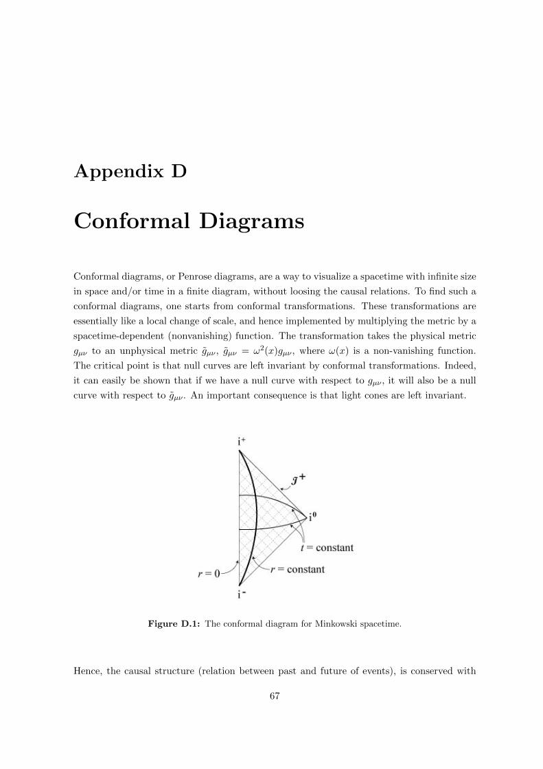
Appendix D

Conformal Diagrams

Conformal diagrams, or Penrose diagrams, are a way to visualize a spacetime with infinite size

in space and/or time in a finite diagram, without loosing the causal relations. To find such a

conformal diagrams, one starts from conformal transformations. These transformations are

essentially like a local change of scale, and hence implemented by multiplying the metric by a

spacetime-dependent (nonvanishing) function. The transformation takes the physical metric

gµ+ to an unphysical metric gµ+ , gµ+ = (2(x)gµ+ , where ((x) is a non-vanishing function.

The critical point is that null curves are left invariant by conformal transformations. Indeed,

it can easily be shown that if we have a null curve with respect to gµ+ , it will also be a null

curve with respect to gµ+ . An important consequence is that light cones are left invariant.

Figure D.1: The conformal diagram for Minkowski spacetime.

Hence, the causal structure (relation between past and future of events), is conserved with

67

Appendix D. Conformal Diagrams 68

conformal transformations. The main rules for a conformal diagram are the same as those of

other spacetime diagrams. A conformal diagram will have a ’timelike’ coordinate, which goes

up, and a ’radial’ coordinate. Light rays travel at 45 degrees. The di!erences lay in the fact

that we aim for coordinates in which infinity is only a finite coordinate value away (so that

the structure of the entire spacetime is immediately apparant), and that almost every point

on the diagram represents a sphere.

Bibliography

[1] R. Bousso. The holographic principle. Rev. Mod. Phys., 74(2):825, 2002.

[2] R. Bousso, B. Freivogel, and S. Leichenauer. Saturating the holographic entropy bound.

Phys. Rev., D82(084024), 2010.

[3] C.E. Shannon. Information in the Holographic Universe. Bell System Technical Journal,

vol. 27:379–423 and 623–656, 1948.

[4] E.T. Jaynes. Information Theory and Statistical Mechanics. The Physical Review,

106(4):620–630, 1957.

[5] J.D. Bekenstein. A mathematical theory of communication. Scientific American,

289(2):61, 2003.

[6] R. Bousso. A covariant entropy conjecture. JHEP, 07(004), 1999.

[7] R. Bousso. Holography in general space-times. JHEP, 06(028), 1999.

[8] S.M. Carroll. Spacetime and geometry. Pearson, 2004.

[9] G.F.R Ellis and H. van Elst. Cosmological models. Mathematical and Physical Sciences,

541:1 , 116, 1999.

[10] J.D. Bekenstein. A universal upper bound on the entropy to energy ratio for bounded

systems. Phys. Rev. D, 289:287, 1981.

[11] N. Kaloper and A. Linde. Cosmology vs. holography. hep-th/9904120, 289, 1999.

[12] W. Fischler and L. Susskind. Holography and cosmology. hep-th/9806039, 1998.

[13] S. Gao and J. Lemos. The covariant entropy bound in gravitational collapse. hep-

th/0403284v2, 2004.

69