Embed Size (px)
Citation preview
The Growth Effects of Tax Rates in the OECD Norman Gemmell, Richard Kneller and Ismael Sanz
WORKING PAPER 2/2013March 2013
Working Papers in Public Finance Chair in Public Finance Victoria Business School

The Working Papers in Public Finance series is published by the Victoria
Business School to disseminate initial research on public finance topics, from
economists, accountants, finance, law and tax specialists, to a wider audience. Any
opinions and views expressed in these papers are those of the author(s). They should
not be attributed to Victoria University of Wellington or the sponsors of the Chair in
Public Finance.
Further enquiries to:
The Administrator
Chair in Public Finance
Victoria University of Wellington
PO Box 600
Wellington 6041
New Zealand
Phone: +64-4-463-9656
Email: [email protected]
Papers in the series can be downloaded from the following website:
http://www.victoria.ac.nz/cpf/working-papers
0
THE GROWTH EFFECTS OF TAX RATES IN THE OECD†
by
Norman Gemmell*+, Richard Kneller*
and Ismael Sanz**
ABSTRACT
The literature testing for aggregate impacts of taxes on long-run growth rates in the OECD
has generally used tax rate measures constructed from macroeconomic aggregates such as
tax revenues. These have a number of advantages but two major disadvantages: they are
typically average, rather than marginal, rates, and are constructed from endogenous tax
revenues. Theory predicts a number of responses to both average and marginal tax rates,
but empirical analogues of the latter tend to be at the micro level. In addition though most
OECD economies are best regarded as small open economies, previous macroeconomic
tests of OECD tax-growth relationships have implicitly been based on closed-economy
models, focusing on domestic tax rates.
This paper explores the relevance of these two aspects – „macro average‟ versus „micro
marginal‟ tax rates, and open economy dimensions – for test of tax-growth effects in
OECD countries. We use annual panel data on a number of average and marginal tax rate
measures and find:
(i) statistically small and/or non-robust effects of macro-based average tax rates on
capital income and consumption but more evidence for average labor income tax
effects;
(ii) statistically robust GDP growth effects of modest size from changes in marginal
income tax rates at both the personal and corporate levels;
(iii) international tax competition, in which both domestic and foreign corporate tax rates
play a role, is consistent with the data;
(v) tax effects on GDP growth appear to operate largely via impacts on factor
productivity rather than factor accumulation.
Keywords: marginal tax rates, average tax rates, personal tax, corporate tax, GDP growth
JEL classification: H24; H30;
Corresponding author: Norman Gemmell ([email protected]); Professor of
Public Finance, Victoria Business School, Victoria University of Wellington, PO box 600,
Wellington 6140, New Zealand..
† We are grateful to participants at the Western Economic Association Annual Conference, Vancouver,
Canada, July 2009, the Victoria University of Wellington, tax conference, Wellington, February 2009, and
seminar participants at the Universities of Oxford, Oregon and Canterbury. We also thank Peren Arin
(Massey), Bob Reed (Canterbury) and Joe Stone (Oregon), for helpful comments on earlier drafts of this
paper. * University of Nottingham, UK; + Victoria University of Wellington, New Zealand; ** Universidad Rey Juan
Carlos, Madrid, Spain.
1
1. Introduction
The empirical literature testing for the effects of taxes on long-run growth have generally
been motivated by two foundational endogenous growth models. The first, Barro (1990)
established a so-called „inverted-U‟ relationship between steady-state growth and income tax
rates in a model in which a „distortionary‟ proportional tax on (capital and labor) income and a
„non-distortionary‟ consumption tax financed a mixture of utility-enhancing and private
production-enhancing public expenditures.
Secondly, focusing more on the tax side of the government budget, a suite of related models
by Devereux and Love (1994, 1995), Roubini and Milesi-Ferretti (1994a, b), Mendoza, Milesi-
Ferretti and Asea (1997), and Milesi-Ferretti and Roubini (1998) established steady-state growth
effects of labor and capital income and consumption taxes in endogenous growth models with
physical and human capital. These papers demonstrated that whether – and how much – each of
those taxes affect long-run growth depends on how „leisure‟ is specified in individuals‟ utility
functions, and the „technology‟ of human capital production.1 The key public finance
characteristics of these models are that growth effects depend on the form of taxation, the type of
public expenditure that is tax-financed and the „technology‟ of goods and human capital
production.
These models have subsequently proved popular as a basis for empirical testing. In the case of
the Barro model this partly reflects the convenience of the „distortionary/non-distortionary‟ tax
and „productive/non-productive‟ expenditure distinctions for identifying empirical proxies; see,
for example, Kneller et al. (1999), Bleaney et al. (2001), Adam and Bevan (2005), Arnold (2008)
and Gemmell et al. (2011). In addition, Mendoza, Milesi-Ferretti and Asea (1997) – hereafter
MMA (1997) – suggested a convenient method for estimating tax rates on capital and labor
income and consumption, suitable for testing their models on macro data. Following Mendoza,
Razin and Tezar (MRT, 1994), they proposed a method of calculating macro-level effective tax
rates based on estimates of tax revenues and tax bases. Subsequently known as „MRT tax rates‟,
a variety of methodological modifications have been suggested2 and have been used to examine
1 For example, whether both physical and human capital are required to produce human capital. Subsequent
endogenous growth models with taxation include Kaas (2003), Kalyvitis (2003), Zagler and Durnecker (2003), Park
and Philippopoulos (2003), Ho and Wang (2005), and Peretto (2003, 2007). Barro, et al (1995) and Turnovsky (2004)
examine the transitional dynamics of tax-growth effects. Futagami et al. (1993) adapt the Barro (1990) model to allow
for externalities from public capital stocks, rather than public expenditure flows. 2 See, for example, Martinez-Mongay (2000), Carey and Tchilinguirian (2000), Carey and Rabesona (2002), Immervol
(2004), de Haan et al. (2004), and McDaniel (2007).
2
tax-growth effects by, for example, Angelopoulos, et al. (2007), and Romero-Ávila and Strauch
(2008).3
As well as providing a testable theoretical model MMA (1997) provided evidence in support
of „Harberger‟s superneutrality conjecture‟ that “although theory predicts that changes in tax
rates affect investment and growth in the long-run, in practice tax policy is an ineffective
instrument to influence growth” (MMA, p.99). Using their constructed MTR tax rates for an
OECD country panel of 5-yearly averaged data, they found modest effects of capital and labor
income taxes on investment (a 10 percentage point reduction in tax rates generating a 1-2%
increase in investment). However, they found negligible effects on GDP growth a statistically
insignificant 0.1-0.2% increase in GDP growth rates from the same tax reductions.4
Subsequent research on the tax-growth relationship in OECD countries, such as the studies
cited above, has tended to find more evidence of adverse effects of various taxes on growth.5
These subsequent studies have used a variety of tax rates, calculated using different methods,
usually applied to annual or period-averaged data and, in some cases, yielding non-robust results
for tax-growth effects.
It therefore remains unclear how far this evidence overturns, or confirms, the original MMA
(1997) conclusion that tax policy is largely incidental for long-run GDP growth rates. In
particular, criticisms leveled at the current evidence include:
1. The potential endogeneity of tax rates calculated from tax revenues – both MRT tax rates
and the „implicit‟ average tax rates obtained from revenue/GDP ratios.
2. Both these are average tax rates. While traditional models of labor supply, and more
recent models of foreign direct investment (FDI), suggest roles for both average and
marginal tax rates, most theoretical macro tax-growth models focus on marginal effects,
though generally from models with proportional taxes, where average and marginal rates
are equal (Li and Sarte, 2005, is an exception).
3 McDaniel (2011) also applies MRT tax rates to aggregate-level tests of labor supply responses. Earlier Barro and
Sahasakul (1983, 1986) proposed using an income-weighted „average marginal tax rate‟ (AMTR) as a suitable macro-
level equivalent of the marginal tax rates normally used to capture individuals‟ labor supply responses to changes in tax
rates. Using this measure, Barro and Redlick (2011) find evidence of lower growth in the US in association with higher marginal tax rates. The method however is data intensive, requiring annual income distribution data for example, and
therefore is not readily applied to large panel datasets. 4 MMA (1997) acknowledge however that, using annual data, they did find some (unreported) evidence of statistically
significant effects of taxes on GDP growth. They interpret this as evidence of transitional growth effects. 5 In addition, if the 0.2% increase in growth estimated by MMA (1997), albeit with a large margin of error, was realized
over the long-run – say, from 2.0% p.a. to 2.2% p.a. - GDP would be around 4% higher after 20 years, and 6% higher
after 30 years. Though not large, these are also not trivial improvements over the counterfactual. Gemmell et al. (2011)
also caution against considering the growth effects of tax changes without also considering the growth effects of other
simultaneous changes in expenditures, deficits or other taxes, mandated by the government budget constraint.
3
3. The empirical literatures on FDI and innovation have focused on the impacts of corporate
or personal tax rates (with potential effects on GDP) rather than the capital/labor
distinction of much of the macro tax-growth literature.
4. Recent tax-growth models such as Peretto (2003, 2007), and empirical studies by Lee and
Gordon (2005), and Arnold et al. (2011), have proposed or examined tax effect on GDP
transmitted via innovation and entrepreneurship effects on multi-factor productivity
instead of, or as well as, via investment.
This paper addresses each of those aspects. We explore GDP responses to both aggregate
average and micro-level marginal tax rates using both capital/labor and personal/corporate
distinctions, and we examine how far estimated tax-growth effects are transmitted via investment
or productivity. In addition, we examine the implications of theoretical open-economy growth
models, such as Roubini and Milesi-Ferretti (RMF, 1994b), for tests of GDP responses to capital
tax rates; in particular focusing on the role of international tax competition and
capital/technology flows.
The remainder of the paper is organized as follows. Section 2 summarizes the relevant tax-
growth theory including open-economy growth aspects. Section 3 discusses the choice of
suitable tax rates and other issues that arise when „taking theory to the data‟. Section 4 first
presents some evidence on the various tax rates for our sample of OECD countries, then
discusses our regression results. Section 5 concludes.
2. Taxes and Growth in Closed and Open Economies: Theory
This section summarizes the main elements of the closed economy MMA (1997) endogenous
growth model, as extended to incorporate foreign investment, following RMF (1994b). Since the
former model at least is well-known, we only sketch its main components here.
MMA (1997) set out a model in which a composite good, Y, and human capital, H, are each
produced from inputs of human and physical capital, K, using CRS technology. Thus:
( ) ( ) (1)
and ,( ) - ( ) (2)
where 1-v (z) is the share of physical (human) capital devoted to human capital accumulation,
and u is the share of human capital used in goods production. Both types of capital depreciate at
rate , and physical capital accumulates according to:
(3)
4
where C is consumption and G is government expenditure (= tax revenues net of any transfers).6
Each individual‟s time endowment is normalized to unity, with (1 – z – u) the fraction of leisure
time. Individuals maximize their lifetime utility based on a CES instantaneous utility function
having consumption, C, and leisure, l, as arguments.
MMA (1997) solve the first order conditions for this problem to obtain the balanced growth
equilibrium. This uses the familiar „fundamental growth equation‟:
( )
(( ) ) (4)
in which the equilibrium growth rate of consumption, , is the difference between the rate of time
preference, , and the net after-tax rate of return on capital, r, adjusted by the inverse of the
intertemporal elasticity of substitution in consumption, . Also, in (4) is the rate of capital
income tax, and RK is the pre-tax rate of return. It is useful to note three further conditions (in (5)
to (7) below) used to derive the semi-reduced form expression for the growth rate in (8): These
are:7
( ) .
/
(5)
( ) .( )
/
( ) (6)
( )
( )
(7)
Hence:
{[ ( ) ( )( ) ( ) ]
} (8)
where D is a function of the production function parameters A, B, and . Together (5) – (8)
demonstrate both the direct effect of both K and H
on growth (as shown in (8)) and the indirect
effects - through (u + z) in (8), and operating through the factor ratios, vK/uH and (1-v)K/zH (as
seen in (5), (6) and (7)). Though the consumption tax rate, C, does not appear explicitly in (5) –
(8), MMA show that C affects the value of ( ) to the extent that there are labor supply
effects. However, as RMF (1994a) demonstrate, if leisure is „quality time‟ or it represents „home
production‟ (both of which embody human capital), or if labor supply is inelastic ( = 0), the
term in (u + z) drops out of (6) and (8) and there are no indirect growth effects from changes in
C.
6 Note that G does not enter either firms‟ productions functions, nor the household‟s utility function. 7 See MMA (1997) for further discussion of the derivation of these conditions.
5
RMF (1994b) extend this model to capture small open economy aspects by allowing (a)
perfect international mobility of capital, but immobile human capital; and (b) the government to
fund its expenditures from bond issues and taxation of foreign assets (based on the residence
principle) at rate, F. The economy takes the world interest rate, r
*, as given, and domestic bonds
and foreign assets are perfect substitutes. Thus net of tax rates of return are equated, introducing
an additional expression for r in equilibrium growth:
( ) . (9)
It follows from the definitions of r in (4) and (9), that in equilibrium the interest rate on
bonds, r, must equal the net-of-tax return on capital and the net-of-tax return on foreign assets.
Further, from (9), it is not possible to set F, K
, and H independently in equilibrium since:
(10)
where, from (4) and (8), r is equal to:
[ ( ) ( )( ) ( ) ]
(11)
Therefore, tax rates on foreign and domestic assets, and human capital, are positively
correlated. Other things equal, a rise in K, for example, will reduce the net-of-tax return on
domestic investment and require an increase in F to avoid arbitrage opportunities leading to an
outflow of capital.8 As Rebelo (1992) notes, this residence-based (or „worldwide‟) tax system in
it‟s pure form implies capital tax rates determined by max(K, F
), where credits are given for any
foreign taxes up to the value of domestic tax liabilities.9 In such a system, the growth effects of
domestic taxes continue to apply.10
However, in the RMF (1994b) model, the introduction of a
territorial tax system (as operates in some EU countries, Australia, New Zealand), in which
foreign income is exempt from domestic taxation, implies that all capital locates abroad in
equilibrium when K > F
, and vice versa for K < F
. Hence steady state growth is unaffected by
changes in tax rates in this case (and there are no transitional dynamics).
In practice, most countries‟ tax systems for foreign capital income are neither pure
„residential‟ nor „territorial‟ systems, and often differentiate between capital income earned
8 Note that, since ( ) ( ) , the tax rates on domestic and foreign assets need not be equal in
equilibrium. However, where fiscal depreciation allowances are set such that ( )( ), then perfect
capital mobility ensures that and (assuming the same consumer preferences and technology across countries). 9 This system is „worldwide‟ since all of a resident‟s income is taxed domestically regardless of where it is earned. It is
used in the US and UK, for example. 10 This is because if (K > F), then K
will apply and there is no foreign tax-induced incentive to invest, while if K < F,
then F applies, and no investment abroad would occur.
6
under personal and corporate tax codes. As a result, in most countries F is determined by a
combination of tax rates set domestically and set abroad, depending for example on treatment of
non-domestic assets, the use of withholding taxes, availability of foreign tax credits, whether tax
is levied on accrual or on repatriation, etc. Hence setting of F in conjunction with domestic tax
rates as described above may not be straightforward, even where the objective is to set those
rates to maximize growth in equilibrium.
A limitation of each of the models described above is that government expenditure affects
neither utility nor goods productions. The Barro model does this. It omits a human capital
production process, and labor supply is exogenous, but adds „productive‟ government spending,
G, to the production function (effectively replacing uH in (1)), with an income tax at rate Y
funding total public spending: hence Y = G/Y.
11 There are constant returns to total „public plus
private capital‟ (though public expenditure is a flow rather than a capital „stock‟), and firms take
government productive spending as given in making their decisions. Hence the fundamental
growth equation (4) above becomes:
{ ( ) ( ) }
* ( )( ) + (12)
where g = G/Y, and { ( ) ( ) } in (12) is the net-of-depreciation, after-tax return
on capital. Here income taxes can be seen to have non-linear effects on growth, due to the
combined effect of reductions in investment, via ( ), and increased investment via the
positive externality effect of government spending: ( ) . An important aspect of (12) for
empirical testing is that, where government productive expenditure is controlled for, tax effects
on long-run growth are expected to be negative, whereas if government expenditure is not
controlled for, a non-linear, inverted-U relationship is expected.
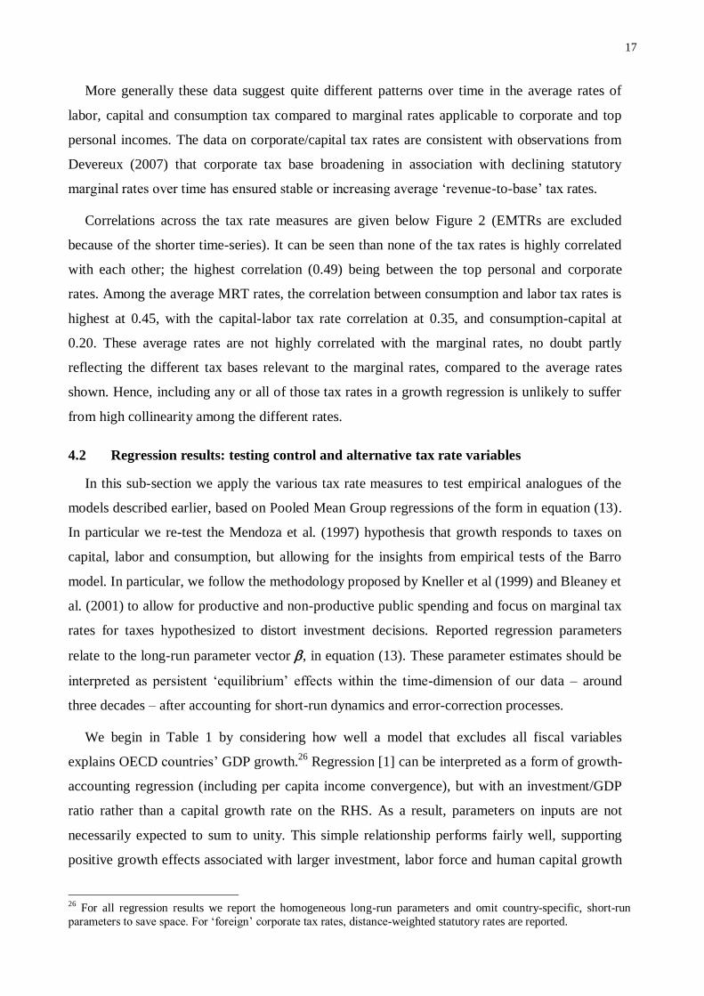
The relationship between steady-state growth and the various tax rates can readily be
illustrated for a set of parameter values in the above equations. Rather than simulate a particular
economy, parameter values have been chosen to yield sensible values for real long-run growth
rates (around 2-3%) at income tax rates around 0.2 to 0.4.12
Using fairly standard values for key
parameters, such as elasticities for production functions, rates of substitution, time preference etc
(see Appendix 1), Figure 1A simulates the relationship between growth and tax rates K, H
, and
11 Barro suggests treating K as „broad capital‟, potentially including human capital. As a result his income tax rate is
implicitly a uniform rate on both labor and capital income. In an extension to the basic model, Barro (1990, p.S117-
118) also adds utility-enhancing government spending and a consumption tax. 12 In particular, having established suitable parameter values for the MMA simulations, the technology parameter, A, in
the Barro production function was selected such that the Barro model yields the same growth rate as the MMA model
when labor and capital income tax rates equal 20%.
7
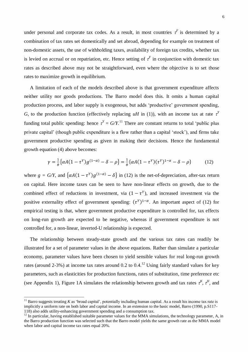
Y, using equation (8) or (12). The Figure shows that, as capital and labor tax rates are raised in
the MMA model, growth rates decline. Unsurprisingly, the rate of decline is greatest when both
capital and labor rates increase, and is least when only labor income tax rates increase. This latter
effect depends, of course, on the respective magnitudes of the assumed responses of capital and
labor to tax rate changes. The profile shown for the Barro model reveals the inverted-U pattern
with the adverse growth effects of income taxes dominating in this case at rates in excess of
around 0.25.
Figure 1A
Figure 1B
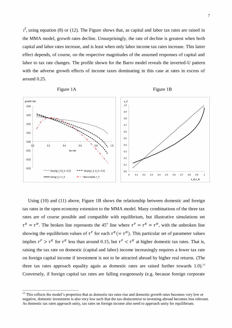
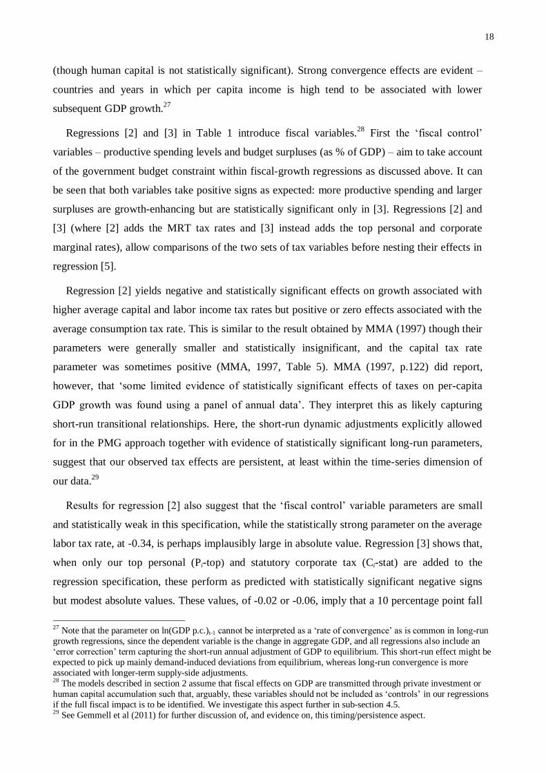
Using (10) and (11) above, Figure 1B shows the relationship between domestic and foreign
tax rates in the open economy extension to the MMA model. Many combinations of the three tax
rates are of course possible and compatible with equilibrium, but illustrative simulations set
. The broken line represents the 45o line where , with the unbroken line
showing the equilibrium values of for each ( ). This particular set of parameter values
implies for less than around 0.15, but at higher domestic tax rates. That is,
raising the tax rate on domestic (capital and labor) income increasingly requires a lower tax rate
on foreign capital income if investment is not to be attracted abroad by higher real returns. (The
three tax rates approach equality again as domestic rates are raised further towards 1.0).13
Conversely, if foreign capital tax rates are falling exogenously (e.g. because foreign corporate
13 This reflects the model‟s properties that as domestic tax rates rise and domestic growth rates becomes very low or
negative, domestic investment is also very low such that the tax-disincentive to investing abroad becomes less relevant.
As domestic tax rates approach unity, tax rates on foreign income also need to approach unity for equilibrium.
-0.03
-0.02
-0.01
0.00
0.01
0.02
0.03
0.04
0.0 0.2 0.4 0.6 0.8 1.0
growth rate
tax rate
Varying t_h (t_k = 0.2) Varying t_k (t_h = 0.2)
Varing t_k = t_h Barro model, t_Y
0.0
0.1
0.2
0.3
0.4
0.5
0.6
0.7
0.8
0.9
1.0
0 0.1 0.2 0.3 0.4 0.5 0.6 0.7 0.8 0.9 1
_F
_K, _H
8
rates are declining and domestic firms‟ foreign investment income is not fully taxed at a higher
domestic rate) then domestic tax rates will also have to fall to maintain equilibrium growth.
3. Taking Theory to the Data
The models described in section 2 identify circumstances in which empirical investigations
could be expected to identify a negative correlation between long-run growth rates and a
combination of domestic taxes on capital and labor income, foreign income and, possibly
consumption. However, they are silent on a number of other empirically important aspects.
Average versus Marginal Effects
All those models treat tax systems as proportional so that marginal and average tax rates are
equal. Clearly this is not the case in practice. Furthermore various theoretical arguments would
lead us to expect different responses to marginal versus average rates. Labor supply responses at
extensive and intensive margins are an obvious example, with implications for long-run output
levels or growth rates. In addition, following Devereux and Griffith (1998, 2003), it is
recognized that firms‟ investment location decisions will be more influenced by the effective
average rate of corporate tax on investment. The effective marginal rate is, however, likely more
relevant to subsequent investment choices, conditional on location, while choices over the
location of profit across tax jurisdictions are more influenced by the statutory corporate rate (see
de Mooij and Ederveen, 2008; Huizinga and Laeven, 2008).
These considerations suggest that which tax rates are relevant to an analysis of the impact of
taxation on GDP growth will depend on the particular decision margins such as labor supply and
investment, which may differ across countries, time and circumstances. Hence empirical testing
should potentially examine both rates in an effort to disentangle the role of each or at least allow
for either to have an impact.
Macro versus Micro Tax Rates and Endogeneity
A major advantage of the MRT (1994) tax rates for macro-level growth studies is that these
tax rates capture average tax rates at that macro level whilst also being based on a clear
conceptual measure of tax wedges – pre-tax and post-tax prices. Hence changes in those rates
might be expected to capture the overall effect of changes in observed average tax burdens on
economic activity. However like the „implicit average tax rates‟ (IATRs) which are based on a
measure of tax revenue relative to GDP, the MRT rates rely on tax revenues for their
construction. Both potentially suffer from endogeneity to the extent that observed tax revenues
are derived from the ex post tax base which, in turn, includes responses to any changes in
9
statutory or effective tax rates at the micro level. Nevertheless the MRT rates are conceptually
superior to the IATRs by avoiding the compounding effects of endogenous GDP responses
relative to tax base responses.
Micro-based tax rate measures, on the other hand, such as the statutory or effective rates faced
by individual suppliers of labor, investors or firms, are probably a better conceptual measure of
the tax rate that induces a behavioral response by the individuals in question. But it remains
unclear which micro-based rates are likely to be most relevant and how pervasive their effects
are likely to be at the macro level. For example, if the top marginal tax rate is increased by 10
percentage points but the average revenue-based MRT labor tax rate changes very little, it is
unclear what lies behind these differences. It may reflect large and widespread negative
behavioral responses to the increased top rate which largely cancel out the direct increase in
revenues, or there may be negligible responses to the marginal rate increase, or the relevant
taxpayers affected may simply be small in overall revenue terms, when viewed at the macro
level.
There is therefore a trade-off between using micro-based tax rates that are relatively less
contaminated by endogeneity concerns than macro-based tax rates, but which are capturing tax
changes of unknown salience at the macro level. Ideally nested regression models that allow for
output responses to both types of tax rate may provide some insight into their relative merits. We
pursue this in section 4.
Finally, recent research on the macroeconomic effects of taxes has increasingly focused on
foreign direct investment (FDI).14
To the extent that these responses predominate among broader
capital income responses, corporate rates become more relevant – either statutory or effective.
Further, the recent evidence of Devereux et al. (2008) provides strong support for the view that,
since the early 1980s, OECD countries have increasingly competed over corporate tax rates
(statutory and effective) to attract mobile capital. If this has spillover effects onto aggregate
economic growth, any reduced-form relationship between domestic tax rates and GDP growth
rates may miss out on a key determinant, namely the interaction between domestic, and
competing foreign, tax rates.
The Devereux et al. evidence is also consistent with the prediction of the open-economy
endogenous growth models discussed above; namely, that in equilibrium, tax rates on foreign-
sourced and domestically-sourced capital will be jointly endogenously determined. These
theoretical models generally have no transitional dynamics: introducing taxes induces an
14 See Blonigen (2005) and de Mooij and Ederveen (2008) for reviews.
10
immediate shift to a new equilibrium. But testing for international tax aspects empirically,
especially with annual data, needs to recognize that over shorter periods international capital tax
rates may diverge from equilibrium settings and induce temporary investment flows with
potential impacts on GDP. Furthermore, in a „many country‟ context, and with international
competition over tax rates, it is less clear how tax rates on domestic and foreign investment can
be set in conjunction in equilibrium. The foreign rates consistent with growth maximization are
likely to vary, depending for example, on the main sources and destinations of FDI and other
capital flows.
Devereux et al. (2008) argue that OECD data supports evidence of increasing openness over
time for many countries but that some remain more insulated from international flows. For this
latter category, domestic tax rates would be expected to assume a greater importance, relative to
other countries‟ settings. Overall, this literature suggests that trying to identify empirically the
respective roles of foreign and domestic tax rates on FDI or GDP is likely to be complicated by
the heterogeneity of circumstances that apply across countries and time.
Growth Effects via Investment or Productivity
As noted in the Introduction, the channel by which taxes affect GDP in the theoretical models
described in section 2 is generally investment in physical and human capital. However, a number
of more recent theoretical models, or a priori arguments, have stressed productivity-related
channels though which taxes may affect GDP. For example, Peretto (2003, 2007), and Lee and
Gordon (2005) argue for tax-growth effects via impacts on innovation or entrepreneurship.
Arnold et al. (2011) provide some empirical support for tax effects on productivity at the firm
level.
While this does not undermine evidence obtained from observing the reduced-form
relationship between taxes and GDP growth, it does suggest that evidence on the direct
relationship between taxes and investment is not the only, nor necessarily most important, means
by which taxes can affect GDP growth. In section 4 we therefore look for tax effects on GDP
growth using three alternative approaches. (i) Examining reduced-form regressions in which tax
rates enter regressions either with, or without, investment variables; (ii) the direct impact of tax
rates on investment; and (iii) allowing capital and other inputs to impact on GDP in a „first stage‟
then test for tax effects directly on this „residual‟ growth variable (a form of multi-factor
productivity growth).
The Government Budget Constrain (GBC)
11
As the Barro (1990) model emphasizes, and most recent tests now recognize, it is important to
accommodate the GBC when testing empirically for an aggregate impact of taxes on growth.
That is, since the government budget is a „closed system‟, any change in one element must be
accompanied by equivalent changes in at least one other element. As a result, any government
budget items not included in the estimating equation are implicitly the funding elements
associated with the included budget categories. Recent empirical tests of the impact of fiscal
variables on growth have, following Barro (1990), typically summarized these as
„distortionary‟/„non-distortionary‟ taxes, „productive‟/ „unproductive‟ expenditures and budget
deficits; see Gemmell et al (2011), Adam and Bevan (2005).
Previous use of implicit‟ tax rates (IATRs), measured by revenues/expenditures/deficits as
ratios of GDP, allow the GBC to be specified „exactly‟ in growth regressions with one or more
categories omitted (the implicit financing) to avoid perfect collinearity.15
However, when
statutory or effective marginal or average tax rates are used in regressions the „omitted financing
element‟ is less clear, making appropriate interpretation of parameters less obvious. To reduce
this problem, we always include budget deficits and „productive‟ public spending as „fiscal
controls‟ in regressions reported below.
Control Variables
Controlling for non-fiscal determinants of growth is not straightforward. Most previous
exercises have attempted to control for standard growth model determinants: labor, capital (more
usually, investment rates) and human capital, with or without various other macro variables
(inflation, trade openness, convergence effects, etc). However, since taxes are hypothesized to
impact on output partly via physical and/or human capital investment, arguably these controls
will capture some of the fiscal effects of interest, leaving only productivity-transmitted effects to
be picked up by tax rate variables. This problem is compounded when poor proxies are relied on
to measure fiscal impacts.
We therefore begin by comparing regressions respectively with/without fiscal or control
variables. We use four control variables: labor force growth, human capital growth (measured as
years of schooling embodied in the labor force)16
, the ratio of private non-residential investment
to GDP, and (the log of) lagged per capita GDP to capture convergence effects. Finally, the
limited availability of some fiscal data limits our sample coverage to 15 OECD countries, data
15 Kneller et al (1999) recommend omitting unproductive spending and/or non-distortionary taxes from such
regressions – since theory suggests these should have little or no growth effect, making interpretation of parameters on
included fiscal variables easier. 16 The human capital data is based on Arnold et al (2007). We are grateful to Jens Arnold, Andrea Bassanini and
Stefano Scarpetta at the OECD for supplying the data.
12
for most countries spanning the late-1970s to 2004.17
To facilitate comparisons across
specifications we generally use a common set of countries in all regressions. Using effective tax
rate data limits the sample to 12 countries from 1980.
Econometric Methods
Our analysis uses two methodologies applied to annual panel data. Firstly, we use the pooled
mean group (PMG) methodology proposed by Pesaran et al (1999). This allows a dynamic
specification in which short- and long-run effects differ, and heterogeneous constants and
marginal short-run effects across countries can be accommodated, while maintaining
homogeneity of the long-run responses. The major advantage of this approach is that it makes
full use of the available time-series information and provides estimates of long-run parameters
without the need for long lag structures. For similar regressions - but based on IATRs - Gemmell
et al. (2011) and Arnold et al. (2011) report that the PMG estimator performs better than
alternative dynamic fixed-effects or mean group (MG) estimators in this context.
Concern over endogeneity is perhaps the major source of unease over the reliability of
previous tests of tax rates on growth, despite various attempts to control for this. Pesaran (1997)
contends that the PMG approach continues to be applicable even if the independent variables are
endogenous, so that valid asymptotic inferences can be made on the short-run and long-run
parameters from this method.18
Nevertheless, given limitations in the PMG‟s ability to deal with
endogeneity via contemporaneous feedbacks between git and Fit in (3), in small samples, where
relevant we further test the robustness to our results to possible endogeneity.19
Our use of statutory and effective rates alongside revenue-based measures makes our
estimates less vulnerable to these endogeneity concerns. Nevertheless, governments‟
discretionary tax changes are sometimes made in response to macroeconomic conditions or, we
have argued, other countries tax rates. Some regressions therefore use instrumental variable
methods based on various weighted averages of other countries’ corporate tax rates, described
further in section 4.
The resulting regression equation which we estimate by PMG or IV methods is of the
following „error correcting‟ form:
17 The full country sample is: Australia*, Austria*, Canada*, Denmark, Finland*, France*, Germany*, Netherlands*,
New Zealand, Norway*, Spain*, Sweden*, Turkey, UK*, USA*. Most regressions use 15 countries; an asterisk
indicates the country is included in the reduced 12 country sample when effective corporate tax rates are used. 18 Indeed Pesaran and Smith (1995) argue that the assumption of homogeneity of the short-run parameter estimates
across countries is a more serious problem in the DFE estimator than the bias generated by the inclusion of lagged
dependent variables and can lead to inconsistent and misleading results even for large T and large N. 19 See Pesaran (1997, pp.182-184) for further discussion.
13
tikti
K
kki
M
mmtimititiiti FgFgg ,,
0,
1,,1,1,, )(
(13)
where i denotes the country, t is time, g is the rate of growth of GDP, F is a matrix of fiscal and
control variables and i,t is a classical error term. The parameter vectors i and respectively
capture the error correction and (homogeneous) long-run growth effects, while i,mand i,k
capture the heterogeneous short-run responses to g and F respectively (with lag lengths M, K =
1). We focus on results for the long-run parameter vector, , which identifies whether fiscal and
other effects on g persist into the long-run. That is, a value of ≠ , implies that any observed
short-run effects observed in the annual data do not decay towards zero over the „long-run‟.
Rather, non-zero effects persist within the time period of around 30 years in our dataset.
Tax Rate Data
The OECD sample coverage – of countries and years - is largely determined by overlaps in
available datasets for tax, other fiscal, and „control‟ variables. Average tax rates for capital, labor
and consumption are the MRT-type rates calculated by McDaniel (2007), and used in McDaniel
(2011), for a sub-sample of OECD countries, based on the original MRT (1994) approach and
the later amendments from Carey and Rabesona (2002).
Marginal tax rate measures are more difficult because suitable macro-based estimates are
generally only available for cross-section or long-run period-averaged data.20
Using micro-based
rates requires choices over which, of several possible, tax rates. These marginal rates are
generally available for „personal‟ and „corporate‟ tax categories rather than capital/labor/
consumption distinctions.
For personal income taxes, because of their wide availability, we use the top statutory
personal income tax rates from the Office of Tax Policy Research (ITPR) at the University of
Michigan, and the OECD Tax Database. We regard these as primarily measures of marginal tax
rates on labor income though equivalent rates on personal capital income are often similar. 21
When used in regressions in conjunction with an average tax rate (such as the MRT rate on labor
income) these marginal rates might be expected to capture a combination of the effects of labor
income tax progressivity and/or tax base broadening/narrowing.
20 Studies such as Padovano and Galli (2002) for example, estimate „aggregate‟ marginal tax rates by regressing tax
revenues on an income measure over a number of years. The resulting parameter is then used as a marginal tax rate
proxy in cross section/panel growth regressions. 21 Some data for statutory marginal personal capital income tax rates (e.g. on interest and dividend income) are
available for OECD countries but coverage is generally limited both across countries and annually. OECD (2012) data
on top rates of personal tax on dividend income are highly correlated (across counties) with top personal rates on
earned income. For 2007, for example, personal MTRs on dividend and wage income are correlated across our 17
country sample at r = 0.75. Data from Tables I.4 & II.4 at www.oecd.org/ctp/taxdatabase.
14
For corporate-level capital income tax rates we use (i) the statutory corporate rate at central
and (where available) sub-central level from the OECD Tax Database; and (ii) the „forward-
looking‟ effective average and marginal tax rates (EATRs, EMTRs) calculated by Devereux et al
(2002) and updated by the Institute for Fiscal Studies (IFS, 2005). These effective rates are
estimated for hypothetical firm-level investments in different countries and years based on
information, for example, on statutory rates, effective depreciation allowances, type of financing,
inflation and interest rates, etc.
By using these rates we hope to capture effects on GDP indirectly through investment, FDI,
productivity or profit-shifting. Any effect on corporate profit-shifting would generally have little
direct effect on real economic activity - to the extent that they represent pure accounting effects
via transfer pricing. However, as Grubert and Slemrod (1998) argue, real resource transfers by
multinationals are often complimentary to profit-shifting strategies. In addition, countries‟
measured GDP will be affected, even if real activity is unchanged, to the extent that shifted
profits are captured in National Accounting profit measures and other output/input price effects.
Foreign Tax Rates
We have argued that foreign corporate tax rates are potentially relevant to domestic
investment decisions, and should therefore be included in an empirical growth model. For each
country in the sample we construct a weighted average of statutory tax rates, EATRs and
EMTRs, in other countries. In their analysis of corporate tax competition, Devereux et al. (2008)
use countries‟ GDP and recent FDI flows as weights.22
We use as weights: (a) the inverse of
distance; (b) GDP; and (c) unweighted; i.e. equal weight. 23
Since the „economic distance‟ that
influences corporate responses to international tax differences may be reflected in a variety of
factors, we explore all three of these weighting schemes.
In fact, we find that (a) and (c) behave similarly and mainly report results for the distance-
weighted case. GDP-weighting generates unreliable estimates, probably because GDP-weighting
leads to an emphasis on just a few countries. Of the 15 countries included in most of our
regressions, the US accounts for around 50% of total GDP, with 75% accounted for by just four
countries: the US, Germany, UK, France. If, as Devereux et al (2008) argue, tax competition
causes country i’s tax rates to react to country j‟s tax-setting choices and vice versa, then
22 With 15 countries and around 30 annual observations, we do not have sufficient degrees of freedom in our panel
regressions to include each „foreign‟ country‟s tax rate separately. 23 We do not use FDI data due to limited availability for early years of our sample. Physical distance is measured by
the inverse of distance between the capital cities of all sample countries. This means, for example, that for a country
such as New Zealand, Australia takes a 95% weight compared to a 5% weight for other countries – reflecting the
likelihood for New Zealand‟s case that flows to/from Australia dominate the potential gains/losses from international
inflows or outflows. Data on New Zealand‟s investment in/out-flows suggest this is the case.
15
individual country corporate tax rates are endogenous. Their empirical solution is to instrument
directly for each country‟s tax rate using the determinants of other sample counties‟ tax rates.
We follow a similar approach, discussed further in section 4.
Finally, if foreign tax rates are important, this may include countries outside our OECD
sample. Obvious examples would be developing country tax havens though, for those countries,
profit-shifting is often alleged to be the primary tax response – with a more tenuous connection
to GDP growth rates. Unfortunately, to include foreign tax rates for a wider group of countries
requires annual data on all the relevant tax rate variables used in our analysis and these are
generally unavailable on a consistent annual basis.24
We therefore do not include additional non-
OECD country tax rates, but recognize that our included foreign tax rate variables may be
proxying for a wider group of relevant countries. Since international trade and investment data
suggest that intra-OECD flows (and FDI stocks) dominate total world flows/stocks, we expect
any effects of omitting other foreign country tax rate variables to be small.
4. Empirical Results
4.1 Trends in tax rate data
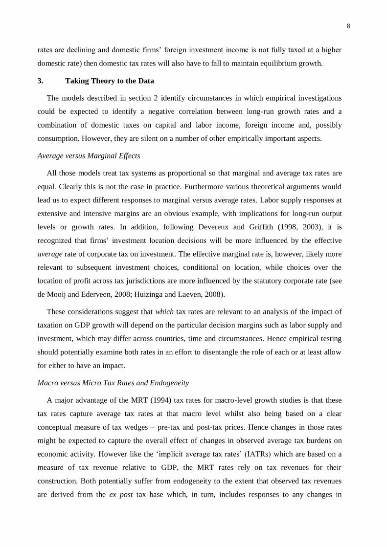
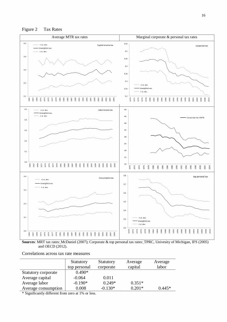
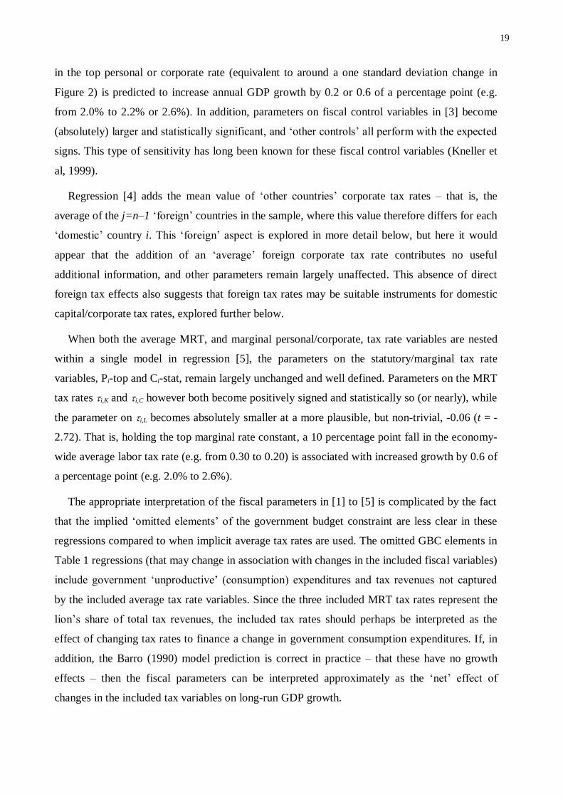
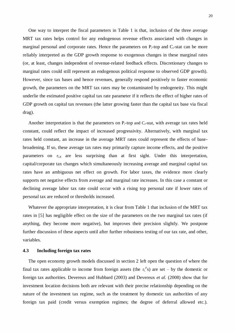
Figure 2 shows average MRT tax rates for consumption, capital and labor income (left-hand
panels) from McDaniel (2007), and the statutory/effective corporate, and top statutory personal
income tax rates (right-hand panels). The figure shows unweighted averages for our sample
countries and one sample standard deviation bands.25
The figure indicates a clear tendency for average consumption and labor tax rates to rise since
the mid-1970s but no similar trend for capital tax rates. Sample statutory corporate tax rates can
be seen to begin a downward trend from the late 1980s, initially fairly rapidly, then more steadily
and this appears to be continuing. This pattern is also reflected in the IFS (2005) data on EMTRs,
with a substantial decline (on average) during the 1980s but a relatively flatter profile in the
1990s. A similar picture emerges for the top personal tax rate with a rapid decline phase
throughout the 1980s and modest declines thereafter.
24 As with our included foreign tax rate variables, each additional foreign tax rate variable would need to be constructed
such that values differs across each in-sample country, otherwise it becomes a form of country fixed effect. In addition
the use of the PMG regression method, which estimates separate short-run responses for each variable and country,
means that each additional variable included in regressions substantially reduces degrees of freedom. 25 Averages are for 13 or 14 of the sample countries. No data are available for Iceland and Luxembourg and the time-
series for Turkey is too short. A Data Appendix showing other individual country tax rates is available from the
authors. See McDaniel (2007) for derivation of her MRT rates, country-specific results and comparisons with the
original MRT (1994) measures.
16
Figure 2 Tax Rates
Average MTR tax rates Marginal corporate & personal tax rates
Sources: MRT tax rates: McDaniel (2007); Corporate & top personal tax rates: TPRC, Univesity of Michigan, IFS (2005)
and OECD (2012).
Correlations across tax rate measures
Statutory
top personal
Statutory
corporate
Average
capital
Average
labor
Statutory corporate 0.490*
Average capital -0.064 0.011
Average labor -0.190* 0.249* 0.351*
Average consumption 0.008 -0.130* 0.201* 0.445* * Significantly different from zero at 1% or less.
0.1
0.2
0.3
0.4
0.5
19
65
19
67
19
69
19
71
19
73
19
75
19
77
19
79
19
81
19
83
19
85
19
87
19
89
19
91
19
93
19
95
19
97
19
99
20
01
20
03
20
05
20
07
20
09
+1 st. dev.
Unweighted ave.
-1 st. dev.
Capital income tax
0.2
0.25
0.3
0.35
0.4
0.45
0.5
0.55
19
70
19
72
19
74
19
76
19
78
19
80
19
82
19
84
19
86
19
88
19
90
19
92
19
94
19
96
19
98
20
00
20
02
20
04
20
06
20
08
20
10
+1 st. dev.
Unweighted ave.
-1 st. dev.
corporate tax
0.0
0.1
0.2
0.3
0.4
0.5
19
65
19
67
19
69
19
71
19
73
19
75
19
77
19
79
19
81
19
83
19
85
19
87
19
89
19
91
19
93
19
95
19
97
19
99
20
01
20
03
20
05
20
07
20
09
+1 st. dev.
Unweighted ave.
-1 st. dev.
Labor income tax
10
15
20
25
30
35
40
45
50
1970
1972
1974
1976
1978
1980
1982
1984
1986
1988
1990
1992
1994
1996
1998
2000
2002
2004
Corporate tax EMTR
0.0
0.1
0.2
0.3
0.4
19
65
19
67
19
69
19
71
19
73
19
75
19
77
19
79
19
81
19
83
19
85
19
87
19
89
19
91
19
93
19
95
19
97
19
99
20
01
20
03
20
05
20
07
20
09
+1 st. dev.
Unweighted ave.
-1 st. dev.
Consumption tax
0.2
0.3
0.4
0.5
0.6
0.7
0.8
19
70
19
72
19
74
19
76
19
78
19
80
19
82
19
84
19
86
19
88
19
90
19
92
19
94
19
96
19
98
20
00
20
02
20
04
20
06
20
08
20
10
+1 st. dev.
Unweighted ave.
-1 st. dev.
top personal tax
17
More generally these data suggest quite different patterns over time in the average rates of
labor, capital and consumption tax compared to marginal rates applicable to corporate and top
personal incomes. The data on corporate/capital tax rates are consistent with observations from
Devereux (2007) that corporate tax base broadening in association with declining statutory
marginal rates over time has ensured stable or increasing average „revenue-to-base‟ tax rates.
Correlations across the tax rate measures are given below Figure 2 (EMTRs are excluded
because of the shorter time-series). It can be seen than none of the tax rates is highly correlated
with each other; the highest correlation (0.49) being between the top personal and corporate
rates. Among the average MRT rates, the correlation between consumption and labor tax rates is
highest at 0.45, with the capital-labor tax rate correlation at 0.35, and consumption-capital at
0.20. These average rates are not highly correlated with the marginal rates, no doubt partly
reflecting the different tax bases relevant to the marginal rates, compared to the average rates
shown. Hence, including any or all of those tax rates in a growth regression is unlikely to suffer
from high collinearity among the different rates.
4.2 Regression results: testing control and alternative tax rate variables
In this sub-section we apply the various tax rate measures to test empirical analogues of the
models described earlier, based on Pooled Mean Group regressions of the form in equation (13).
In particular we re-test the Mendoza et al. (1997) hypothesis that growth responds to taxes on
capital, labor and consumption, but allowing for the insights from empirical tests of the Barro
model. In particular, we follow the methodology proposed by Kneller et al (1999) and Bleaney et
al. (2001) to allow for productive and non-productive public spending and focus on marginal tax
rates for taxes hypothesized to distort investment decisions. Reported regression parameters
relate to the long-run parameter vector , in equation (13). These parameter estimates should be
interpreted as persistent „equilibrium‟ effects within the time-dimension of our data – around
three decades – after accounting for short-run dynamics and error-correction processes.
We begin in Table 1 by considering how well a model that excludes all fiscal variables
explains OECD countries‟ GDP growth.26
Regression [1] can be interpreted as a form of growth-
accounting regression (including per capita income convergence), but with an investment/GDP
ratio rather than a capital growth rate on the RHS. As a result, parameters on inputs are not
necessarily expected to sum to unity. This simple relationship performs fairly well, supporting
positive growth effects associated with larger investment, labor force and human capital growth
26 For all regression results we report the homogeneous long-run parameters and omit country-specific, short-run
parameters to save space. For „foreign‟ corporate tax rates, distance-weighted statutory rates are reported.
18
(though human capital is not statistically significant). Strong convergence effects are evident –
countries and years in which per capita income is high tend to be associated with lower
subsequent GDP growth.27
Regressions [2] and [3] in Table 1 introduce fiscal variables.28
First the „fiscal control‟
variables – productive spending levels and budget surpluses (as % of GDP) – aim to take account
of the government budget constraint within fiscal-growth regressions as discussed above. It can
be seen that both variables take positive signs as expected: more productive spending and larger
surpluses are growth-enhancing but are statistically significant only in [3]. Regressions [2] and
[3] (where [2] adds the MRT tax rates and [3] instead adds the top personal and corporate
marginal rates), allow comparisons of the two sets of tax variables before nesting their effects in
regression [5].
Regression [2] yields negative and statistically significant effects on growth associated with
higher average capital and labor income tax rates but positive or zero effects associated with the
average consumption tax rate. This is similar to the result obtained by MMA (1997) though their
parameters were generally smaller and statistically insignificant, and the capital tax rate
parameter was sometimes positive (MMA, 1997, Table 5). MMA (1997, p.122) did report,
however, that „some limited evidence of statistically significant effects of taxes on per-capita
GDP growth was found using a panel of annual data‟. They interpret this as likely capturing
short-run transitional relationships. Here, the short-run dynamic adjustments explicitly allowed
for in the PMG approach together with evidence of statistically significant long-run parameters,
suggest that our observed tax effects are persistent, at least within the time-series dimension of
our data.29
Results for regression [2] also suggest that the „fiscal control‟ variable parameters are small
and statistically weak in this specification, while the statistically strong parameter on the average
labor tax rate, at -0.34, is perhaps implausibly large in absolute value. Regression [3] shows that,
when only our top personal (Pi-top) and statutory corporate tax (Ci-stat) are added to the
regression specification, these perform as predicted with statistically significant negative signs
but modest absolute values. These values, of -0.02 or -0.06, imply that a 10 percentage point fall
27 Note that the parameter on ln(GDP p.c.)t-1 cannot be interpreted as a „rate of convergence‟ as is common in long-run
growth regressions, since the dependent variable is the change in aggregate GDP, and all regressions also include an
„error correction‟ term capturing the short-run annual adjustment of GDP to equilibrium. This short-run effect might be
expected to pick up mainly demand-induced deviations from equilibrium, whereas long-run convergence is more
associated with longer-term supply-side adjustments. 28 The models described in section 2 assume that fiscal effects on GDP are transmitted through private investment or
human capital accumulation such that, arguably, these variables should not be included as „controls‟ in our regressions
if the full fiscal impact is to be identified. We investigate this aspect further in sub-section 4.5. 29 See Gemmell et al (2011) for further discussion of, and evidence on, this timing/persistence aspect.
19
in the top personal or corporate rate (equivalent to around a one standard deviation change in
Figure 2) is predicted to increase annual GDP growth by 0.2 or 0.6 of a percentage point (e.g.
from 2.0% to 2.2% or 2.6%). In addition, parameters on fiscal control variables in [3] become
(absolutely) larger and statistically significant, and „other controls‟ all perform with the expected
signs. This type of sensitivity has long been known for these fiscal control variables (Kneller et
al, 1999).
Regression [4] adds the mean value of „other countries‟ corporate tax rates – that is, the
average of the j=n–1 „foreign‟ countries in the sample, where this value therefore differs for each
„domestic‟ country i. This „foreign‟ aspect is explored in more detail below, but here it would
appear that the addition of an „average‟ foreign corporate tax rate contributes no useful
additional information, and other parameters remain largely unaffected. This absence of direct
foreign tax effects also suggests that foreign tax rates may be suitable instruments for domestic
capital/corporate tax rates, explored further below.
When both the average MRT, and marginal personal/corporate, tax rate variables are nested
within a single model in regression [5], the parameters on the statutory/marginal tax rate
variables, Pi-top and Ci-stat, remain largely unchanged and well defined. Parameters on the MRT
tax rates i,K and i,C however both become positively signed and statistically so (or nearly), while
the parameter on i,L becomes absolutely smaller at a more plausible, but non-trivial, -0.06 (t = -
2.72). That is, holding the top marginal rate constant, a 10 percentage point fall in the economy-
wide average labor tax rate (e.g. from 0.30 to 0.20) is associated with increased growth by 0.6 of
a percentage point (e.g. 2.0% to 2.6%).
The appropriate interpretation of the fiscal parameters in [1] to [5] is complicated by the fact
that the implied „omitted elements‟ of the government budget constraint are less clear in these
regressions compared to when implicit average tax rates are used. The omitted GBC elements in
Table 1 regressions (that may change in association with changes in the included fiscal variables)
include government „unproductive‟ (consumption) expenditures and tax revenues not captured
by the included average tax rate variables. Since the three included MRT tax rates represent the
lion‟s share of total tax revenues, the included tax rates should perhaps be interpreted as the
effect of changing tax rates to finance a change in government consumption expenditures. If, in
addition, the Barro (1990) model prediction is correct in practice – that these have no growth
effects – then the fiscal parameters can be interpreted approximately as the „net‟ effect of
changes in the included tax variables on long-run GDP growth.
20
One way to interpret the fiscal parameters in Table 1 is that, inclusion of the three average
MRT tax rates helps control for any endogenous revenue effects associated with changes in
marginal personal and corporate rates. Hence the parameters on Pi-top and Ci-stat can be more
reliably interpreted as the GDP growth response to exogenous changes in these marginal rates
(or, at least, changes independent of revenue-related feedback effects. Discretionary changes to
marginal rates could still represent an endogenous political response to observed GDP growth).
However, since tax bases and hence revenues, generally respond positively to faster economic
growth, the parameters on the MRT tax rates may be contaminated by endogeneity. This might
underlie the estimated positive capital tax rate parameter if it reflects the effect of higher rates of
GDP growth on capital tax revenues (the latter growing faster than the capital tax base via fiscal
drag).
Another interpretation is that the parameters on Pi-top and Ci-stat, with average tax rates held
constant, could reflect the impact of increased progressivity. Alternatively, with marginal tax
rates held constant, an increase in the average MRT rates could represent the effects of base-
broadening. If so, these average tax rates may primarily capture income effects, and the positive
parameters on i,K are less surprising than at first sight. Under this interpretation,
capital/corporate tax changes which simultaneously increasing average and marginal capital tax
rates have an ambiguous net effect on growth. For labor taxes, the evidence more clearly
supports net negative effects from average and marginal rate increases. In this case a constant or
declining average labor tax rate could occur with a rising top personal rate if lower rates of
personal tax are reduced or thresholds increased.
Whatever the appropriate interpretation, it is clear from Table 1 that inclusion of the MRT tax
rates in [5] has negligible effect on the size of the parameters on the two marginal tax rates (if
anything, they become more negative), but improves their precision slightly. We postpone
further discussion of these aspects until after further robustness testing of our tax rate, and other,
variables.
4.3 Including foreign tax rates
The open economy growth models discussed in section 2 left open the question of where the
final tax rates applicable to income from foreign assets (the i,Fs) are set – by the domestic or
foreign tax authorities. Devereux and Hubbard (2003) and Devereux et al. (2008) show that for
investment location decisions both are relevant with their precise relationship depending on the
nature of the investment tax regime, such as the treatment by domestic tax authorities of any
foreign tax paid (credit versus exemption regimes; the degree of deferral allowed etc.).
21
Importantly, Devereux and Hubbard (2003) develop a model in which profit-maximizing firms
choose between exporting to, or investing in, foreign countries. They show that, whether foreign
tax rates are higher or lower than in the domestic economy is important in determining whether,
and where, firms invest abroad.
Appendix 2 provides an illustration based on the Devereux and Hubbard model. This
demonstrates that, at least under the more common „foreign tax credit‟ system (with or without
deferral), whereby taxes paid abroad are partially credited against domestic tax liabilities,
investing in foreign assets in lower tax countries is strongly favored over investing in higher tax
countries. Importantly, this shows that if both „high tax‟ and „low tax‟ foreign countries reduce
their tax rates, but country tax rate rankings do not change, investment is incentivized to move to
the „low tax‟ country but not (or less so) to the „high tax‟ country despite both having reduced
their tax rates. This process underlies the hypothesized „race to the bottom‟ in corporate tax
competition. It may be expected to affect GDP growth directly through the inflows of foreign
investment and enhanced technology (productivity), and the indirect spillover effects on
domestic firms.
These asymmetric effects of foreign inflows suggest the possibility that, in assessing effects
on investment or productivity (and hence growth), the foreign country tax rates relevant to any
individual country, i, may differ depending on that countries position in the international ranking
of capital tax rates. In particular, among the j=n-1 „foreign‟ countries, changes in capital tax
rates in country j, when tj,K > ti,K, may have less impact on investment and technology flows
between i and j than when tj,K < ti,K.
To explore this possibility, we construct foreign country averages of corporate tax rates, as
described in section 3, but distinguishing between those countries (and years) where tj,K > ti,K, and
those where tj,K < ti,K, using the statutory (or effective) corporate tax rate to measure tK. In our
regression analysis we refer to these tax rates as Cj-stat-L and Cj-stat-H respectively for „low‟
and „high‟ tax countries. Note that, if an individual country‟s corporate tax rate falls or rises over
time such that its position in the cross-country ranking changes, the composition of countries in
its Cj-stat-L and Cj-stat-H averages will also change.
We use these tax rates in three ways. Firstly, if foreign corporate tax rates exert an
independent influence on GDP growth, they may be added to our previous regressions.
Secondly, if international corporate rates are set inter-dependently (as seems likely at least for
more open OECD economies) we need to allow for this inter-dependence of corporate rates.
Thirdly, a plausible alternative hypothesis (and one that is consistent with the theoretical
22
modeling earlier) is that foreign tax rates have no direct impact on GDP, but only via their
effects on the setting of domestic corporate rates. This can be tested by instrumenting for Ci-stat
using the foreign average rates, rather than including those foreign rates directly in the growth
regression.
Table 1 shows the results of testing foreign corporate tax rates. We begin by omitting the
MRT variables from the PMG regression in [6] and replacing Cj-stat from regression [3] with
both Cj-stat-H and Cj-stat-L. Regression [7] expands [6] by adding the MRT tax rates for labor
and capital. These regressions continue to support the previous negative association between
growth and the top personal, and domestic corporate, tax rates. MRT tax rates on capital and
labor continue to take positive and negative signs respectively but are not statistically significant
(at 10%). The parameters on Cj-stat-H and Cj-stat-L suggest, as predicted, a positive association
between the tax rate in „low tax‟ foreign countries and domestic growth rates with effectively no
association with Cj-stat-H. However, neither parameter is statistically strong.
When we omit the domestic corporate rate, Ci-stat in [8] – effectively assuming only foreign
tax rates directly determine domestic GDP growth – the results for Cj-stat-L are unchanged, but
Cj-stat-H is now statistically significant. This strongly suggests that the effects of Cj-stat-H, the
foreign corporate tax rate, on growth operate at least in part through Ci-stat, its domestic
counterpart. If domestic rates are determined by foreign tax rates, such that the latter affect GDP
growth only indirectly, we can instrument for Ci-stat using the foreign corporate tax rate
averages. We do this in the instrumental variable regressions, [9] and [10] (see Table 2) using Cj-
stat-L (both distance-weighted and GDP-weighted): the parameter on Ci-stat continues to be
robustly negative and similar in magnitude to previous regression estimates. Parameters for the
MRT tax rates also become more robustly estimated though larger (in absolute value) and signs
remain negative (positive) for the labor (capital) average tax rate.30
Finally regressions [11] and [12] omit our control for private non-residential investment. If
most of the impact of taxes on GDP growth is through investment responses, then omitting
investment should increase the observed association between the fiscal variables and GDP
growth – compared with the equivalent regressions [9] and [10]. In fact, parameters on our
marginal tax rates remain largely unaffected while those on the MRT average tax rates become
30 IV diagnostics shown below Table 2 support the instruments chosen. We also examine IV regressions in which we
instrument additionally for the MRT tax rates (using „low tax‟ countries weighted MTR rates as instruments), other
fiscal variables and investment. Since the only additional instruments available for other fiscal variables and investment
are the 3rd/4th lagged (predetermined) values, we do not place a great deal of weight on these results. Nevertheless, the
parameters and statistical significance of our various tax rate measures remain similar to those given in Tables 1 & 2.
23
absolutely smaller. This would seem to suggest that, to the extent that fiscal variables are
associated with GDP growth, the primary mechanism is not via investment.31
The regressions in Tables 1and 2 therefore provide broad support for the conclusion that
lower GDP growth tends to be associated with higher personal, and domestic corporate, marginal
tax rates. There is also a positive association between GDP growth and corporate tax rates in
foreign countries initially below the country of interest. However, these latter effects may best be
thought of as occurring through their effect on domestic corporate rates. For example, for a given
country i, as foreign corporate rates fall over time, they simultaneously drive down country i's
corporate rate. For labor tax rates, results generally support the view that higher average and
marginal tax rates (the latter captured by the top personal rate) are each associated with lower
GDP growth. In all cases these results relate to long-run parameters suggesting that observed
annual changes tend to persists over several years.32
4.4 Results using effective corporate tax rates
In Table 3 we report on the impact of capital tax rates on growth using the forward-looking
effective average and marginal corporate tax rates from IFS (2005). These effective rates are
hypothetical rates applicable to specified investment types undertaken under alternative
assumptions regarding, for example, the relevant rate of interest, inflation rate, method of
financing (debt, equity) etc. IFS (2005) calculate ETRs using a number of alternative
assumptions for each year for 12 of the countries in our sample.33
These measures of taxation have the advantage over actual tax rates (revenue-based or
otherwise), that they do not include the response to current or past changes in policy. For that
reason they might reasonably be regarded as genuinely exogenous though, of course, they are not
„macro‟ tax rates and may therefore not provide a suitable proxy for „aggregate‟ capital tax rates
changes. They are also available for a more limited sample of countries and years. Nevertheless,
in view of their exogeneity properties we consider them as measures of average and marginal
capital tax rates – at the corporate level. In view of the arguments that, for many investment
location decisions, it is the average, rather than marginal, tax rate that is relevant, we consider 31 This is confirmed when we replace GDP growth with the investment rate as our dependent variable. In this case,
unlike MMA (1997), we find no significant effects of our tax rates on investment – though we would caution that such regressions are somewhat ad hoc in specification and are not derived from a fully-specified model of the determinants
of investment. 32 This evidence is consistent with Romer and Romer (2010) who found, using VAR methods, that strong negative
impacts of income tax rates on US GDP estimated for up to 5 years, appeared to persist beyond this period. 33 Table 3 reports regressions for the case of assumed uniform inflation rates across countries. Other assumptions are:
investment is in plant and machinery, financed by equity or retained earnings, taxation at shareholder level is not
included, rate of economic rent = 10% (i.e. financial return = 20%), real discount rate = 10%, inflation rate = 3.5%,
depreciation rate = 12.25%; see Devereux and Griffith (2003) for details. We also obtained results using ETRs
calculated using each country‟s own inflation rate; results are similar.
24
both effective rates. However, there are two important limitations on the use of these effective
rates.
Firstly, the average and marginal rate measures tend to be highly correlated within countries.
34 To minimize this effect in our regressions we include the EMTR, and the difference between
the EMTR and EATR. When an EMTR is included in regressions, parameters on the difference
variable should therefore be interpreted as the impact of changes in the effective average tax rate,
for a given effective marginal rate. The effect of EMTR changes will be captured by both
parameters. Since corporate taxes tend not to display progressive structures, in these data an
increase in the EATR, for a given EMTR, primarily reflects base broadening via limitations to
corporate tax deductions such as depreciation allowances.
Secondly, these country- and year-specific effective tax rate measures tend to move together
over time, in part because their construction involves some common components, such as annual
inflation and interest rates. As a result testing for separate responses to „foreign‟ and „domestic‟
effective tax rates is likely to be less reliable. To help combat this we generally enter our EMTRi,
EMTRj-H, EMTRi-L variables only one (or at most two) at a time in regressions.
Table 3 reports regressions similar to those in Table 1 but using these effective average or
marginal corporate tax rates. We focus first on results for labor tax rates. Results for the top
marginal income tax rate, Pi-top, can be seen to be consistently negative and significant in Table
3 regressions, with parameter estimates, around –0.02 to –0.04, that are similar to, or (absolutely)
slightly smaller than, those in Tables 1 and 2. Unlike the top personal rate, the parameters on the
average MRT tax rate for labor, i,L appears to be non-robustly estimated in Table 3, with
estimates varying between –0.02 and +0.25.
For corporate effective tax rates however, consistent with the results from Table 2, regression
(1) in Table 3 confirms a negative association between a county‟s EMTRi and GDP growth, but a
positive association with EMTRjs in foreign „low tax‟ countries (EMTRj-L). When the domestic
EMTRi is omitted and EMTRj-H is introduced in regression (2), this appears to have little effect
on the estimated parameter on EMTRj-L, while the parameter on EMTRj-H confirms no
additional effect on growth from those „high tax‟ countries.
Regressions (3) and (4) introduce the EATRi difference variable (EMTRi – EATRi), with and
without EMTRi. Firstly, these regressions confirm a positive, statistically significant parameter
associated with low tax foreign countries, EMTRj-L, at around –0.05. Secondly when both
34 In this sample the EATRs and EMTRs are highly correlated overall: r = 0.90 to 0.98 (for the 3 weighting cases)
across the 12 OECD countries.
25
EMTRi and (EMTRi – EATRi) are included in (4) it is clear the primary association between
effective tax rates and growth is via the difference between the EMTRi and EATRi. This is
confirmed by comparing regressions (1) and (3): in regression (3) where EMTRi is excluded the
parameter estimate on (EMTRi – EATRi) is –0.075, and exceeds that on EMTRi of –0.35 in (1)
where (EMTRi – EATRi) is excluded.35
Despite the limitations noted above on these EMTR/EATR variables and sample, these results
offer surprisingly robust confirmation of those in Tables 1 and 2; namely that the top marginal
labor tax rate is robustly negatively associated with GDP growth, while results for the average
labor tax rate are less clear. Similarly, domestic and foreign corporate tax rates are respectively
negatively and positively associated with GDP growth, as found earlier. These corporate-level
capital tax rates would appear to be more consistently associated with GDP growth with the
expected signs.
4.5 Further specification testing
In this, and the next, sub-sections we investigate the sensitivity of our results to the
inclusion/exclusion of various macroeconomic control variables. We previously demonstrated
that our tax results appear not to be sensitive to excluding private non-residential investment
from our regressions. Here we investigate the impact of (a) omitting the lagged GDP per capita
„convergence‟ term; (b) adding other macro controls – inflation and trade openness; and (c)
omitting all foreign tax effects. Sub-section 4.6 examines the effects of allowing all macro input
variables (investment, labor force and human capital) to impact on growth first and then test for
tax effects on the resulting „residual‟ measure of multi-factor productivity growth. As a
benchmark we use PMG regression [7] in Table 1 - which includes all foreign and domestic tax
rates (except the average consumption tax rate).
Results are shown in the right-hand columns of Table 2, which repeats regression [7] for
comparison. In regression [13], omitting the per capita income convergence term, ln(GDP p.c.)t-1,
has no impact on the signs, and little impact on the statistical significance, of the personal
marginal tax rate or the various corporate tax rates – though Ci-stat-L now becomes highly
statistically significant. However, both the labor and capital average MTR tax rates appear to be
sensitive to this change in specification – with changes in parameter signs and standard errors. It
would seem therefore that these „macro‟ tax rates are sensitive to the inclusion/exclusion of other
macro controls but our „micro‟ tax rates are not.
35 The parameter estimates on (EMTRi – EATRi) in (3) and (4) imply that raising the EATR, whilst holding the EMTR
constant, has a positive association with GDP growth. We interpret this as an income effect from the implicit
inframarginal increase in depreciation deductions associated with the EATR rise.
26
A number of recent studies, such as Lee and Gordon (2005) and Angelopoulos et al (2007)
have added further macroeconomic control variables to their fiscal-growth regression – mainly
inflation rates and trade openness variables (but have ignored the „openness‟ aspect to corporate
tax impacts). When we add those variables to Table 1 regressions (not shown in Table 2), using
[5] and [7] which respectively exclude and include foreign taxes, we find little effect on the sign
or statistical significance of the parameters on our tax rate variables, while the inflation and
openness variables enter with the expected signs (negative and positive respectively) or are close
to zero.
We noted earlier that adding a combined „foreign corporate tax rate‟ in regression [4] was
largely redundant, while including „low‟ and „high‟ tax regimes supported the inclusion of the
former. In regression [14] all foreign corporate tax rates are omitted and it can be seen that the
parameter on the domestic corporate rate is little affected – but with a slightly smaller point
estimate and smaller variance compared to [7]. Since this parameter estimate is also similar to
that obtained using IV methods (based on foreign tax instruments) in regressions [9] and [10],
this would suggest that results for the corporate tax rate are highly robust to alternative
approaches to capturing their effect on long-run domestic GDP growth rates. As suggested by
Devereux et al. (2008), a high degree of co-determination of these foreign/domestic rates seems
plausible.
4.6 ‘Residual growth’ regressions
As noted above, tax rate effects on growth may operate primarily through factors such as
innovation and entrepreneurship that affect factor productivity, and our earlier evidence seems to
suggest that the identified tax effects did not operate via physical capital investment. Of course,
omission of investment from growth regressions may induce omitted variable bias whenever
these control variables are a function of non-tax, as well as tax, variables.36
An alternative is to
disallow any impacts of tax via our control variables and compare the resulting estimates with
those obtained above. To the extent that these parameters are similar, it would suggest that tax
impacts on GDP growth operate primarily through productivity rather than factor inputs.
To test this we use residuals from a regression similar to regression [1] in Table 1 but
excluding the lagged per capita income term. These residuals represent a form of total factor
productivity (TFP) growth measure, being the growth rate of GDP net of any associated changes
36 Ideally, a structural model that sought to model both tax and non-tax determinants of our controls variables could be
used. While such components of such a model are increasingly being pursued at the micro level – e.g. estimating tax
impacts within investment equations – it is because of difficulties fully specifying and estimating such structural
models at the aggregate level that the reduced forms used here have been commonplace in recent literature.
27
in investment, labor and human capital growth. We refer to this as „residual growth‟, gR, and
examine how far our fiscal variables can explain this residual.
Regressions [15] and [16] in Table 2 report PMG regressions for gR specifications that
respectively exclude and include foreign corporate tax rate variables. These regressions may be
compared with the GDP regressions [14] and [7] respectively. We would not suggest that these
regressions represent appropriately specified explanations of total factor productivity growth.
Even a cursory reading of the literature on the determinants of productivity growth identifies
several non-fiscal right-hand-side variables likely to affect TFP in addition to lagged GDP per
capita (R&D expenditure, innovation, distance from „frontier‟ technology, business regulation,
financial market constraints, etc.). Rather, our objective here is to establish whether the tax rate
variables continue to have any explanatory power when our previous control variables are first
allowed maximum effect.
Considering first the case where foreign tax rates are included: compare regressions [16] and
[7]. Parameters on the personal and corporate marginal tax rate variables are largely unaffected.
These are generally close to those obtained for GDP growth – though there is stronger evidence
of a statistically significant direct effect of Cj-stat-L on productivity growth in [16] than on GDP
growth in [7]. Thus, even after attributing maximum effect to „input‟ variables, both personal and
corporate tax rates continue to display statistically strong association with growth via
productivity impacts. These results suggest that the previously estimated GDP impacts of
personal and corporate tax rates operate primarily through productivity effects rather than via
investment etc. Though statistically non-zero, their estimated long-run magnitudes continue to be
modest in size – a 1 percentage point (ppt) change in these tax rates generating around a 0.01 to
0.03 ppt change in long-run residual (TFP) growth rates (e.g. from 2.0% to 2.01% or 2.03%).
For the labor and capital MTR average tax rates, regressions [15] and [16] suggest that these
remain small and statistically non-robust, especially for the average capital tax rate. That is, they
do not reliably identify effects of changes in average tax rates on productivity growth. Similarly,
Table 2 shows that our other fiscal control variables, productive public expenditures and budget
surpluses, generally have no statistically robust impact on long-run TFP growth (unlike their
estimated impact on GDP). This is also a plausible outcome, suggesting that to the extent that
increases in, for example, public infrastructure, health and education expenditures affect output
growth, this is primarily observed in association with increases in investment and human capital
inputs rather than TFP. Finally a comparison of regressions [15] and [16] suggests that,
erroneously omitting the (significant) effects of foreign corporate tax rates leads to an under-
28
estimate of the productivity response to domestic corporate rates, Ci-stat – the latter appearing
close to zero in [15] when Cj-stat-L is omitted from the specification.
5. Conclusions
This paper has sought to deal with two perceived weaknesses in recent aggregate tests of the
impact of taxes on long-run growth rates in OECD countries. First, existing evidence is largely
based on macro measures of average tax rates which are constructed from tax revenue data.
Theoretical aggregate-level growth models generally assume proportional taxes and hence
cannot distinguish between marginal and average tax rates in determining long-run growth. More
specific models (for example, microeconomic models of labor supply or FDI) recognize separate
output effects from average and marginal tax rates. The choice of appropriate tax rates to test
these growth models, and how best to deal with endogeneity associated with tax revenue-based
measures, remain debated issues.
Second, despite increased awareness and testing of corporate tax effects on aggregate growth,
the models previously tested are essentially „closed economy‟ in nature. Based on an open
economy extension of the Mendoza et al. (1997) model, we have proposed an approach to test
how far both domestic and foreign corporate tax settings affect individual countries‟ aggregate
long-run growth rates. Identifying these „foreign‟ tax effects on GDP growth is not
straightforward empirically, but we suggest that such effects may be asymmetric between
countries with corporate tax rates (statutory and/or effective) below, or above, the domestic
equivalent rate.
Based on annual panel data for a sample of 15 OECD countries, we have tested for aggregate
tax-growth effects associated with changes in both macro „Mendoza-Razin-Tezar‟ measures of
average capital and labor tax rates and the more micro-based marginal rates associated with
personal and corporate tax regimes. To the extent possible we have explored both statutory and
effective marginal rates. We find:
(i) Robust evidence that increases in the marginal rate of personal income tax as measured by
the top rate, and (less robustly) the average labor tax rate are associated with adverse long-
run growth outcomes;
(ii) The „macro‟ MRT average tax rates – on consumption, labor and, especially, capital –
generally appear to be less robustly associated with GDP or productivity growth than the
„micro-based‟ marginal tax rates on personal and corporate income.
(iii) Despite methodological difficulties separately identifying both domestic and foreign
corporate tax rate effects on GDP, these appear to have affected OECD growth rates as
29
predicted by open-economy growth models. Particularly strong corporate tax effects
appear to be associated with tax reductions in „lower-tax‟ foreign countries, while
reductions in „higher-tax‟ foreign countries appear of limited relevance for domestic
growth rates. There is some evidence that corporate tax rates are jointly endogenously
determined across countries.
(iv) Like Mendoza et al (1997), we also find no evidence of harmful long-run growth effects
from increases in (average) consumption tax rates.
Our estimates suggest growth effects of a 1 percentage point change in personal or corporate
marginal tax rates that would be observed at the second, not the first, decimal point: e.g. annual
GDP growth rising from 2% to 2.03% not 2.3%. Alternatively, it would need a tax cut such as
from 40% to 30% in the top personal or corporate rate to raise growth from 2.0% to 2.3% over
the long-run, assuming other countries do not follow suit. These results seem plausible to us as
estimates of aggregate tax effects; they imply small but non-trivial effects on GDP levels over
several decades.
Finally, given the difficulties diagnosing the channels by which our micro-based marginal tax
rates might impact on aggregate output measures such as GDP growth, we are not suggesting
that the particular rates we have tested are the key ones associated with GDP growth outcomes.
Rather, we view them as proxies for the various personal and corporate marginal tax rates that
potentially affect output across OECD countries. Future research might usefully construct and
test macro-based marginal tax rates for OECD country panels, such as those developed by Barro
and Sahasakul (1986) and Romer and Romer (2010) for the US. Unfortunately, the detailed
country-specific information requirements to construct such measures make their application to
multi-country samples resource-intensive and difficult to implement consistently.
30
References
Adam, C.S. and Bevan, D.L. (2005) Fiscal deficits and growth in developing countries. Journal
of Public Economics, 89, 571-597.
Angelopoulos, K., Economides, G. and Kammas, P. (2007) Tax-spending policies and economic
growth: theoretical predictions and evidence from the OECD. European Journal of
Political Economy, 23, 885-902.
Arnold, J., Bassanini, A. and Scarpetta, S. (2007): Solow or Lucas? Testing growth models using
panel data from OECD countries. OECD Economics Department Working Paper No.592.
Arnold, J. (2008) Do tax structures affect aggregate economic growth: empirical evidence from
a panel of OECD countries. OECD Economics Department Working Paper No. 643.
Arnold, J., Brys, B., Heady, C., Johannson, A., Schwellnus, C. and Vartia, L. (2011) Tax policy
for economic recovery and growth. Economic Journal, 121, F59-80.
Barro, R. (1990) Government spending in a simple model of endogenous growth. Journal of
Political Economy, 98, s103-117.
Barro, R.J. and Sahasakul, C. (1983) Measuring the average marginal income tax rate from the
individual income tax. Journal of Business, 56, 419-452.
Barro, R.J. and Sahasakul C. (1986) Average Marginal Tax Rates from Social Security and the
Individual Income Tax. Journal of Business, 59, 555-566.
Barro, R.J. and Redlick, C.J (2011) Macroeconomic effects from government purchases and taxes.
Quarterly Journal of Economics, 126, 51-102.
Barro, R., Mankiw, N.G. and Sala-i-Martin X. (1995) Capital mobility in neoclassical models of
growth. American Economic Review, 85, 103-115.
Basmann, R.L. (1960) On Finite Sample Distributions on Generalized Classical Linear
Identifiability Test Statistics. Journal of the American Statistical Association 55, 650–59.
Baum, C., Schaffer, M. and Stillman, S. (2003) Instrumental variables and GMM: Estimation
and testing. Stata Journal, 3, 1-31.
Bleaney, M., Gemmell, N. and Kneller R. (2001) Testing the endogenous growth model: public
expenditure, taxation and growth over the long run. Canadian Journal of Economics, 34,
36-57.
Blonigen, B. (2005) A Review of the Empirical Literature on FDI Determinants. Atlantic
Economic Journal, 33, 383-403.
Carey, D. and Tchilinguirian, H. (2000) Carey, D. and H. Tchilinguirian (2000) Average Effective
Tax Rates on Capital, Labour and Consumption. OECD Economics Department Working
Paper, No. 258. Paris: OECD.
Carey, D. and Rabesona, J. (2002) Tax ratios on labor and capital income and on Consumption.
OECD Economic studies, 35, 2002/2.
De Haan, J., Sturm, J.-E., Volkerink, B. (2004) How to measure the tax burden on labor at the
macro-level? In: Sørensen, P.B. (ed.), Measuring the Tax Burden on Capital and Labor.
Cambridge MA: MIT Press, pp. 289–318.
De Mooij and Ederveen (2008) corporate tax elasticities: a reader‟s guide to empirical findings.
Oxford Review of Economic Policy, 24, 680-697.
Devereux, M.B. and Love, D.R. (1994) The effects of taxation in a two-sector model of
endogenous growth. Canadian Journal of Economics, 27, 509-536.
31
Devereux, M.B. and Love, D.R. (1995) The dynamic effects of government spending policies in
a two-sector endogenous growth model. Journal of Money, Credit and Banking, 27, 232-
256.
Devereux M.P. (2007) Developments in the taxation of corporate profit in the OECD since
1965: rates, bases and revenues. Oxford University Centre for Business Taxation, Working
Paper No. 07/04.
Devereux, M.P., Griffith, R. and Klemm, A. (2002) Corporate income tax reforms and
international tax competition. Economic Policy, 35, 451-495.
Devereux, M.P. and Griffith R. (1998) „Taxes and the location of production: evidence from
a panel of US multinationals‟, Journal of Public Economics, 68 , 335–67 .
Devereux, M.P. and Griffith, R. (2003) Evaluating tax policy for location decisions.
International Tax and Public Finance, 10, 107-126.
Devereux, M.P. and Hubbard, G.R. (2003) Taxing multinationals. International Tax and Public
Finance, 10, 469-487.
Devereux, M.P., Lockwood, B. and Redoano, M. (2008) Do countries compete over tax rates?
Journal of Public Economics, 92, 1210-1235.
European Commission (2000) Public Finances in EMU – 2000. European Economy, Reports and
Studies, 2000/3.
Futagami, K., Morita, Y. and Shibata, A. (1993) Dynamic analysis of an endogenous growth Model
with public capital. Scandinavian Journal of Economics, 95, 607-625.
Gemmell, N., Kneller, R. and Sanz, I. (2011) The timing and persistence of fiscal policy impacts
on growth: Evidence from OECD countries. Economic Journal, 121, F33–F58.
Grubert, H. and Slemrod, J. (1998) The effect of taxes on investment and income shifting to
Puerto Rico. Review of Economics and Statistics, 80, 365-373.
Ho, W.H. and Wang, Y. (2005) Public capital, asymmetric information and economic growth.
Canadian Journal of Economics, 38, 57-80.
Huizinga, H. and Laeven, L. (2008) International profit shifting within multinationals: a multi-
country perspective. Journal of Public Economics, 92, 1164-1182.
Immervoll , H. (2004) Average and Marginal Effective Tax Rates Facing Workers in the EU.
OECD Social, Employment, and Migration Working Papers, No. 19. Paris: OECD.
Institute for Fiscal Studies (2005) Corporate Tax Rate Data. London: IFS. Available at
http://www.ifs.org.uk/publications/3210.
Kaas, L. (2003) Productive government spending, growth, and sequential voting. European
Journal of Political Economy, 19, 227-246.
Kalyvitis, S. (2003) Public investment rules and endogenous growth with empirical evidence
from Canada. Scottish Journal of Political Economy, 50, 90-110.
Kneller, R., Bleaney, M. and Gemmell, N. (1999) Fiscal policy and growth: evidence from
OECD countries. Journal of Public Economics, 74, 171-190.
Lee, Y. and Gordon, R.H. (2005) Tax structure and economic growth. Journal of Public
Economics, 89, 1027-1043.
Li, W. and Sarte, P-D. (2004) Progressive taxation and long-run growth. American Economic
Review, 94, 1705-1716.
32
Martinez-Mongay, C. (2000) ECFIN‟s effective tax rates. Properties and comparisons with other
tax indicators. Economic Paper No. 146 (October). European Commission, Directorate-
General for Economic and Financial Affairs, Brussels.
McDaniel, C. (2007) Average tax rates on consumption, investment, labor and capital in the OECD
1950-2003. Arizona State University.
McDaniel, C. (2011) Forces shaping hours worked in the OECD 1964-2004. American
Economic Journal: Macroeconomics, 3, 27–52.
Mendoza, E., Razin, A. and Tesar , L. (1994) Effective tax rates in macroeconomics: cross-country
estimates on factor income and consumption. Journal of Monetary Economics, 34, 297-323.
Mendoza, E., Milesi-Ferretti G. and Asea P. (1997) On the ineffectiveness of tax policy in
altering long-run growth: Harberger‟s superneutrality hypothesis. Journal of Public
Economics, 66, 99-126.
Milesi-Ferretti, G.M and Roubini, N. (1998) On the taxation of human and physical capital in
models of endogenous growth. Journal of Public Economics, 70, 237-254.
OECD (2012) OECD Tax Database. Centre for Tax Policy and Administration. Available at
www.oecd.org/ctp/taxdatabase.
Padovano, F. and Galli, E. (2002) Comparing the growth effects of marginal vs average tax rates
and progressivity. European Journal of Political Economy, 18, 529-544.
Park, H. and Philippopoulos, A. (2003) On the dynamics of growth and fiscal policy with
redistributive transfers. Journal of Public Economics, 87, 515-538.
Peretto, P.F. (2003) Fiscal policy and long-run growth in R&D-based models with endogenous
market structure, Journal of Economic Growth, 8, 325-347.
Peretto, P.F. (2007) Corporate taxes, growth and welfare in a Schumpeterian economy, Journal of
Economic Theory, 137, 353 – 382.
Pesaran, M. H (1997). The role of economic theory in modelling the long run, Economic Journal,
107, 178-191.
Pesaran M.H. and Smith, R.P. (1995). Estimating long-run relationships from dynamic
heterogeneous panels, Journal of Econometrics, 68, 79-113.
Pesaran, M.H., Shin Y. and Smith R.P. (1999) Pooled Mean Group estimation of dynamic
heterogeneous panels. Journal of the American Statistical Association, 94, 621-34.
Rebelo, S. (1992), Growth in open economies. Carnegie-Rochester Conference Series on Public
Policy, 36, 5-46.
Romer, C.D. and Romer, D.H. (2010) The macroeconomic effects of tax changes: Estimates
based on a new measure of fiscal shocks. American Economic Review, 100(3), 763-801.
Romero-Avila, D. and Strauch, R. (2008) Public finances and long-term growth in Europe:
Evidence from a panel data analysis. European Journal of Political Economy, 24, 172-191.
Roubini, N. and Milesi-Ferretti, G.M (1994a) Optimal Taxation of Human and Physical Capital
in Endogenous Growth Models. NBER Working Papers No.4882. National Bureau of
Economic Research
Roubini, N. and Milesi-Ferretti, G.M. (1994b) Taxation and Endogenous Growth in Open
Economies. NBER Working Papers No.4881. National Bureau of Economic Research.
Sargan, J. (1958) The Estimation of Economic Relationships Using Instrumental Variables,
Econometrica 26,393–415.

33
Shea, J. (1997) Instrument relevance in multivariate linear models: A simple measure. Review of
Economics and Statistics, 79, 348-352.
Staiger, D. and Stock, J. (1997) Instrumental variables regression with weak instruments.
Econometrica, .65, 557-86.
Stock, J. and Yogo, M. (2005) Testing for weak instruments in linear IV regression. In D.W.K.
Andrews and J.H. Stock (eds), Identification and Inference for Econometric Models:
Essays in Honor of Thomas Rothenberg. Cambridge: Cambridge University Press, 80–108.
Turnovsky, S.J. (2004) The transitional dynamics of fiscal policy: Long-run capital accumulation
and growth. Journal of Money, Credit and Banking, 36, 883-910.
Zagler, M. and Durnecker, G. (2003) Fiscal policy and economic growth. Journal of Economic
Surveys, 17, 397-418.
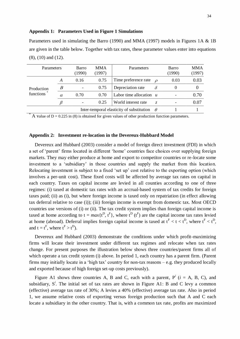
34
Appendix 1: Parameters Used in Figure 1 Simulations
Parameters used in simulating the Barro (1990) and MMA (1997) models in Figures 1A & 1B
are given in the table below. Together with tax rates, these parameter values enter into equations
(8), (10) and (12).
Parameters Barro
(1990)
MMA
(1997)
Parameters Barro
(1990)
MMA
(1997)
Production
functions *
A 0.16 0.75 Time preference rate 0.03 0.03
- 0.75 Depreciation rate 0 0
0.70 0.70 Labor time allocation u - 0.70
- 0.25 World interest rate z - 0.07
Inter-temporal elasticity of substitution 1 1 * A value of D = 0.225 in (8) is obtained for given values of other production function parameters.
Appendix 2: Investment re-location in the Devereux-Hubbard Model
Devereux and Hubbard (2003) consider a model of foreign direct investment (FDI) in which
a set of „parent‟ firms located in different „home‟ countries face choices over supplying foreign
markets. They may either produce at home and export to competitor countries or re-locate some
investment to a „subsidiary‟ in those countries and supply the market from this location.
Relocating investment is subject to a fixed „set up‟ cost relative to the exporting option (which
involves a per-unit cost). These fixed costs will be affected by average tax rates on capital in
each country. Taxes on capital income are levied in all counties according to one of three
regimes: (i) taxed at domestic tax rates with an accrual-based system of tax credits for foreign
taxes paid; (ii) as (i), but where foreign income is taxed only on repatriation (in effect allowing
tax deferral relative to case (i)); (iii) foreign income is exempt from domestic tax. Most OECD
countries use versions of (i) or (ii). The tax credit system implies than foreign capital income is
taxed at home according to t = max{tD, t
F}, where t
D (t
F) are the capital income tax rates levied
at home (abroad). Deferral implies foreign capital income is taxed at tF < t < t
D, where t
F < t
D,
and t = tF, where t
F > t
D).
Devereux and Hubbard (2003) demonstrate the conditions under which profit-maximizing
firms will locate their investment under different tax regimes and relocate when tax rates
change. For present purposes the illustration below shows three countries/parent firms all of
which operate a tax credit system (i) above. In period 1, each country has a parent firm. (Parent
firms may initially locate in a „high tax‟ country for non-tax reasons – e.g. they produced locally
and exported because of high foreign set-up costs previously).
Figure A1 shows three countries A, B and C, each with a parent, Pi (i = A, B, C), and
subsidiary, Si. The initial set of tax rates are shown in Figure A1: B and C levy a common
(effective) average tax rate of 30%; A levies a 40% (effective) average tax rate. Also in period
1, we assume relative costs of exporting versus foreign production such that A and C each
locate a subsidiary in the other country. That is, with a common tax rate, profits are maximized
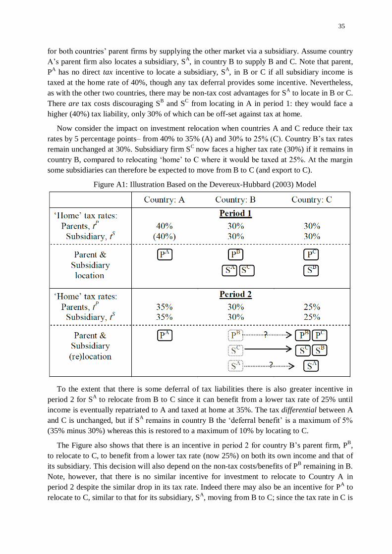
35
for both countries‟ parent firms by supplying the other market via a subsidiary. Assume country
A‟s parent firm also locates a subsidiary, SA, in country B to supply B and C. Note that parent,
PA has no direct tax incentive to locate a subsidiary, S
A, in B or C if all subsidiary income is
taxed at the home rate of 40%, though any tax deferral provides some incentive. Nevertheless,
as with the other two countries, there may be non-tax cost advantages for SA to locate in B or C.
There are tax costs discouraging SB and S
C from locating in A in period 1: they would face a
higher (40%) tax liability, only 30% of which can be off-set against tax at home.
Now consider the impact on investment relocation when countries A and C reduce their tax
rates by 5 percentage points– from 40% to 35% (A) and 30% to 25% (C). Country B‟s tax rates
remain unchanged at 30%. Subsidiary firm SC
now faces a higher tax rate (30%) if it remains in
country B, compared to relocating „home‟ to C where it would be taxed at 25%. At the margin
some subsidiaries can therefore be expected to move from B to C (and export to C).
Figure A1: Illustration Based on the Devereux-Hubbard (2003) Model
To the extent that there is some deferral of tax liabilities there is also greater incentive in
period 2 for SA to relocate from B to C since it can benefit from a lower tax rate of 25% until
income is eventually repatriated to A and taxed at home at 35%. The tax differential between A
and C is unchanged, but if SA remains in country B the „deferral benefit‟ is a maximum of 5%
(35% minus 30%) whereas this is restored to a maximum of 10% by locating to C.
The Figure also shows that there is an incentive in period 2 for country B‟s parent firm, PB,
to relocate to C, to benefit from a lower tax rate (now 25%) on both its own income and that of
its subsidiary. This decision will also depend on the non-tax costs/benefits of PB remaining in B.
Note, however, that there is no similar incentive for investment to relocate to Country A in
period 2 despite the similar drop in its tax rate. Indeed there may also be an incentive for PA to
relocate to C, similar to that for its subsidiary, SA, moving from B to C; since the tax rate in C is
36
now lower at 25%. However since the period 2 tax differential is unchanged in this case (35%
versus 25%), any incentive for PA to relocate will depend on the precise specification of the
fixed costs of relocating (represented in Figure A1 by the “?”).
This illustration serves to highlight that with a tax credit system of foreign capital taxation,
with or without deferral, there are potential incentives for capital to respond to changes in tax
rates in foreign, relative to „home‟, countries. However, these incentives are asymmetric. A
reduction in a „high tax‟ country‟ provides less incentive for investment to move there
compared to a similar reduction in a „low tax‟ country. Rather, ceteris paribus, capital seeks out
the lowest average tax rates across countries subject to the tax and non-tax costs/benefits of
their initial location choices and the fixed costs of relocating versus per unit costs of supplying
foreign markets from home. See Devereux and Hubbard (2003; especially pp.480-484 for
further discussion).
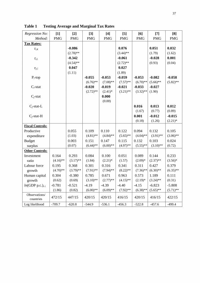
37
Table 1 Testing Average and Marginal Tax Rates
Regression No:
Method:
[1]
PMG
[2]
PMG
[3]
PMG
[4]
PMG
[5]
PMG
[6]
PMG
[7]
PMG
[8]
PMG
Tax Rates:
i,K -0.086 0.076 0.051 0.032
(2.78)** (3.44)** (1.79) (1.62)
i,L -0.342 -0.061 -0.028 0.001
(4.54)** (2.72)** (0.93) (0.04)
i,C 0.047 0.027
(1.11) (1.89)
Pi-top -0.055 -0.053 -0.059 -0.053 -0.082 -0.058
(6.76)** (7.08)** (7.57)** (6.70)** (5.66)** (5.82)**
Ci-stat -0.020 -0.019 -0.021 -0.033 -0.027
(2.72)** (2.41)* (3.21)** (3.32)** (1.90)
Cj-stat 0.000
(0.00)
Cj-stat-L 0.016 0.013 0.012
(1.67) (0.77) (0.89)
Cj-stat-H 0.001 -0.012 -0.015
(0.18) (1.26) (2.21)*
Fiscal Controls:
Productive 0.055 0.109 0.110 0.122 0.094 0.132 0.105
expenditure (1.03) (4.81)** (4.84)** (5.65)** (4.04)** (3.91)** (3.06)**
Budget 0.003 0.151 0.147 0.115 0.132 0.103 0.024
surplus (0.07) (6.44)** (6.00)** (4.97)** (5.55)** (3.10)** (0.72)
Other Controls:
Investment 0.164 0.293 0.084 0.100 0.051 0.089 0.144 0.233
ratio (4.16)** (3.17)** (1.84) (2.21)* (1.57) (2.09)* (2.37)** (3.56)*
Labour force 0.195 0.368 0.301 0.316 0.341 0.311 0.427 0.379
growth (4.70)** (3.79)** (7.91)** (7.94)** (8.22)** (7.36)** (6.30)** (6.35)**
Human capital 0.304 -0.380 0.785 0.671 0.963 0.573 1.189 0.111
growth (0.62) (0.69) (3.10)** (2.77)** (4.15)** (2.19)* (3.24)** (0.31)
ln(GDP p.c.)t-1 -0.781 -0.521 -4.19 -4.39 -4.40 -4.15 -6.823 -5.808
(1.86) (0.82) (6.00)** (6.09)** (7.92)** (6.38)** (5.65)** (5.71)**
Observations/
countries 472/15 447/15 420/15 420/15 416/15 420/15 416/15 422/15
Log likelihood -709.7 -620.8 -544.9 -536.1 -456.3 -522.8 -457.6 -499.4
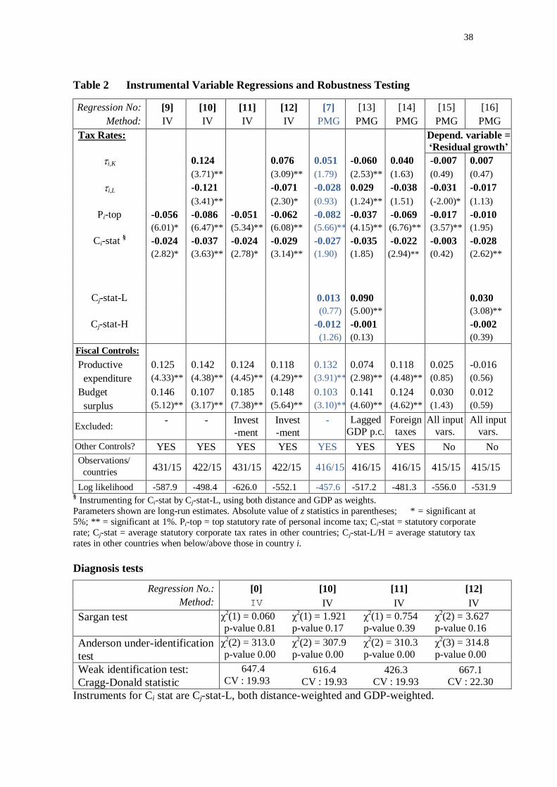
38
Table 2 Instrumental Variable Regressions and Robustness Testing
Regression No:
Method:
[9]
IV
[10]
IV
[11]
IV
[12]
IV
[7]
PMG
[13]
PMG
[14]
PMG
[15]
PMG
[16]
PMG
Tax Rates: Depend. variable =
‘Residual growth’
i,K 0.124 0.076 0.051 -0.060 0.040 -0.007 0.007
(3.71)** (3.09)** (1.79) (2.53)** (1.63) (0.49) (0.47)
i,L -0.121 -0.071 -0.028 0.029 -0.038 -0.031 -0.017
(3.41)** (2.30)* (0.93) (1.24)** (1.51) (-2.00)* (1.13)
Pi-top -0.056 -0.086 -0.051 -0.062 -0.082 -0.037 -0.069 -0.017 -0.010
(6.01)* (6.47)** (5.34)** (6.08)** (5.66)** (4.15)** (6.76)** (3.57)** (1.95)
Ci-stat § -0.024 -0.037 -0.024 -0.029 -0.027 -0.035 -0.022 -0.003 -0.028
(2.82)* (3.63)** (2.78)* (3.14)** (1.90) (1.85) (2.94)** (0.42) (2.62)**
Cj-stat-L 0.013 0.090 0.030
(0.77) (5.00)** (3.08)**
Cj-stat-H -0.012 -0.001 -0.002
(1.26) (0.13) (0.39)
Fiscal Controls:
Productive 0.125 0.142 0.124 0.118 0.132 0.074 0.118 0.025 -0.016
expenditure (4.33)** (4.38)** (4.45)** (4.29)** (3.91)** (2.98)** (4.48)** (0.85) (0.56)
Budget 0.146 0.107 0.185 0.148 0.103 0.141 0.124 0.030 0.012
surplus (5.12)** (3.17)** (7.38)** (5.64)** (3.10)** (4.60)** (4.62)** (1.43) (0.59)
Excluded: - - Invest
-ment
Invest
-ment
- Lagged
GDP p.c.
Foreign
taxes
All input
vars.
All input
vars.
Other Controls? YES YES YES YES YES YES YES No No
Observations/
countries 431/15 422/15 431/15 422/15 416/15 416/15 416/15 415/15 415/15
Log likelihood -587.9 -498.4 -626.0 -552.1 -457.6 -517.2 -481.3 -556.0 -531.9 § Instrumenting for Ci-stat by Cj-stat-L, using both distance and GDP as weights.
Parameters shown are long-run estimates. Absolute value of z statistics in parentheses; * = significant at
5%; ** = significant at 1%. Pi-top = top statutory rate of personal income tax; Ci-stat = statutory corporate
rate; Cj-stat = average statutory corporate tax rates in other countries; Cj-stat-L/H = average statutory tax
rates in other countries when below/above those in country i.
Diagnosis tests
Regression No.: [0] [10] [11] [12]
Method: IV IV IV IV
Sargan test
χ2(1) = 0.060
p-value 0.81
χ2(1) = 1.921
p-value 0.17
χ2(1) = 0.754
p-value 0.39
χ2(2) = 3.627
p-value 0.16
Anderson under-identification
test
χ2(2) = 313.0
p-value 0.00
χ2(2) = 307.9
p-value 0.00
χ2(2) = 310.3
p-value 0.00
χ2(3) = 314.8
p-value 0.00
Weak identification test:
Cragg-Donald statistic
647.4
CV : 19.93 616.4
CV : 19.93
426.3
CV : 19.93
667.1
CV : 22.30
Instruments for Ci stat are Cj-stat-L, both distance-weighted and GDP-weighted.
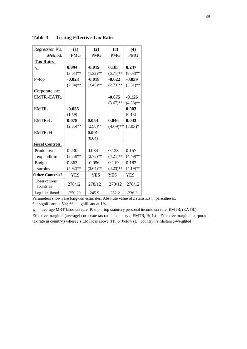
39
Table 3 Testing Effective Tax Rates
Regression No:
Method:
(1)
PMG
(2)
PMG
(3)
PMG
(4)
PMG
Tax Rates:
i,L 0.094 -0.019 0.183 0.247
(3.01)** (1.32)** (6.71)** (8.03)**
Pi-top -0.023 -0.018 -0.022 -0.039
(2.34)** (3.45)** (2.73)** (3.51)**
Corporate tax:
EMTRi-EATRi -0.075 -0.126
(3.67)** (4.38)**
EMTRi -0.035 0.003
(1.59) (0.13)
EMTRj-L 0.078 0.054 0.046 0.043
(2.85)** (2.98)** (4.09)** (2.03)*
EMTRj-H
0.001
(0.04)
Fiscal Controls:
Productive 0.230 0.084 0.123 0.157
expenditure (3.78)** (2.75)** (4.21)** (4.49)**
Budget 0.363 -0.056 0.119 0.182
surplus (5.92)** (3.64)** (4.23)** (4.19)**
Other Controls? YES YES YES YES
Observations/
countries 278/12 278/12 278/12 278/12
Log likelihood -250.20 -245.9 -252.2 -236.3
Parameters shown are long-run estimates. Absolute value of z statistics in parentheses.
* = significant at 5%; ** = significant at 1%.
i,L = average MRT labor tax rate. Pi-top = top statutory personal income tax rate. EMTRi (EATRi) =
Effective marginal (average) corporate tax rate in country i; EMTRj-H(-L) = Effective marginal corporate
tax rate in country j where j‟s EMTR is above (H), or below (L), country i‟s (distance-weighted

Working Papers in Public FinanceChair in Public Finance Victoria Business School
About the Authors Norman Gemmell is Professor of Public Finance at Victoria Business School,Victoria University of Wellington, New Zealand. Email: [email protected] Richard Kneller is Research Fellow in the Centre for Globalisation andEconomic Policy and a professor of Economics at the University of Nottingham.Email: [email protected] Ismael Sanz is Professor of the Department of Applied Economics I at Universidad Rey Juan Carlos.Email: [email protected]