Embed Size (px)
Citation preview
Remote Sens. 2015, 7, 600-626; doi:10.3390/rs70100600
remote sensing ISSN 2072-4292
www.mdpi.com/journal/remotesensing
Article
The Ground-Based Absolute Radiometric Calibration of Landsat 8 OLI
Jeffrey Czapla-Myers 1,*, Joel McCorkel 2, Nikolaus Anderson 1, Kurtis Thome 2,
Stuart Biggar 1, Dennis Helder 3, David Aaron 3, Larry Leigh 3 and Nischal Mishra 3
1 Remote Sensing Group, College of Optical Sciences, University of Arizona, 1630 E University
Blvd, Tucson, AZ 85721, USA; E-Mails: [email protected] (N.A.);
[email protected] (S.B.) 2 NASA Goddard Space Flight Center, Greenbelt, MD 20771, USA;
E-Mails: [email protected] (J.M.); [email protected] (K.T.) 3 Office of Engineering Research, College of Engineering, South Dakota State University, Brookings,
SD 57007, USA; E-Mails: [email protected] (D.H.); [email protected] (D.A.);
[email protected] (L.L.); [email protected] (N.M.)
* Author to whom correspondence should be addressed; E-Mail: [email protected];
Tel.: +1-520-621-4242; Fax: +1-520-621-8292.
Academic Editors: Brian Markham and Prasad Thenkabail
Received: 1 August 2014 / Accepted: 23 December 2014 / Published: 7 January 2015
Abstract: This paper presents the vicarious calibration results of Landsat 8 OLI that were
obtained using the reflectance-based approach at test sites in Nevada, California, Arizona,
and South Dakota, USA. Additional data were obtained using the Radiometric Calibration
Test Site, which is a suite of instruments located at Railroad Valley, Nevada, USA. The
results for the top-of-atmosphere spectral radiance show an average difference of −2.7, −0.8,
1.5, 2.0, 0.0, 3.6, 5.8, and 0.7% in OLI bands 1–8 as compared to an average of all of the
ground-based measurements. The top-of-atmosphere spectral reflectance shows an average
difference of 1.6, 1.3, 2.0, 1.9, 0.9, 2.1, 3.1, and 2.1% from the ground-based measurements.
Except for OLI band 7, the spectral radiance results are generally within ±5% of the design
specifications, and the reflectance results are generally within ±3% of the design
specifications. The results from the data collected during the tandem Landsat 7 and 8 flight
in March 2013 indicate that ETM+ and OLI agree to each other to within ±2% in similar
bands in top-of-atmosphere spectral radiance, and to within ±4% in top-of-atmosphere
spectral reflectance.
OPEN ACCESS

Remote Sens. 2015, 7 601
Keywords: Landsat 8; OLI; radiometric calibration; surface reflectance
1. Introduction
The Landsat Data Continuity Mission (LDCM) was launched on 11 February 2013 from Vandenberg
Air Force Base, and it was renamed Landsat 8 after the transition from the National Aeronautics and
Space Administration (NASA) to the United States Geological Survey (USGS). The platform contains
two instruments: the Operational Land Imager (OLI), and the Thermal Infrared Sensor (TIRS), which
complement one another in spectral coverage. OLI is a visible and near infrared (VNIR) multispectral
sensor that operates from 400–2500 nm, and TIRS is a two-band thermal sensor that operates from
10.6–12.5 μm [1,2]. The in-flight absolute radiometric calibration of OLI is the focus of this work.
Landsat 8 is the latest platform in the 40-year Landsat series of satellites. The VNIR bands retain
many of the characteristics of previous Landsat sensors such as a 185-km swath width, a 30-m ground
instantaneous field of view (GIFOV) for the multispectral bands, and a 15-m GIFOV for the
panchromatic band (Table 1). OLI was developed by the Ball Aerospace and Technology Corporation
in Boulder, Colorado, USA. Significant changes were made in the electro-optical design as compared to
the Enhanced Thematic Mapper Plus (ETM+) on Landsat 7. One prominent change was the transition
from a whiskbroom configuration (ETM+) to a pushbroom configuration, which was successfully
demonstrated by the Earth Observing One (EO-1) Advanced Land Imager (ALI) [3,4]. The pushbroom
configuration allows OLI to have a signal-to-noise ratio (SNR) that is eight times greater than ETM+
when viewing typical radiance levels. OLI has 12-bit radiometric resolution, which is 16 times greater
than the eight-bit data from ETM+. The higher SNR coupled with the higher bit level means that OLI is
able to resolve smaller radiometric differences than ETM+. Although the pushbroom configuration has
a much higher SNR, the radiometric calibration is more complex due to the approximately 7000 detectors
in each of the multispectral bands.
Table 1. The specifications for the spectral bands of ETM+ and OLI used in this work. The
center wavelength is determined by band averaging the relative spectral response (RSR) for
each channel. Note that ETM+ band 6 is thermal, and it is not included here.
OLI ETM+
Band Center Wavelength (nm) Band Center Wavelength (nm)
1 443.0 -- --
2 482.6 1 478.7
3 561.3 2 561.0
4 654.6 3 661.4
5 864.6 4 834.6
6 1609.1 5 1650.3
7 2201.3 7 2208.2
8 (Pan) 591.7 8 (Pan) 720.1
The top-of-atmosphere (TOA) spectral radiance and TOA spectral reflectance are two products
available from OLI, and the calibration traceability follows two separate paths [4,5]. The preflight

Remote Sens. 2015, 7 602
radiometric calibration and SI traceability of OLI was completed using a 27.9-cm spherical integrating
source (SIS), which was calibrated at the Facility for Spectroradiometric Calibration (FASCAL) at the
National Institute of Standards and Technology (NIST). The measurements at NIST were also
independently verified using transfer radiometers from NASA, NIST, the University of Arizona,
and also with the Ball Standard Radiometer (BSR), which is spectrally controlled using filters that match
the RSRs of OLI. When the SIS was returned to Ball Aerospace, it was measured again using Ball’s
radiometer and its own internal monitor. The radiance calibration was then transferred to the large SIS,
nicknamed the Death Star Source (DSS), using Ball’s Commercial-Off-The-Shelf (COTS) Transfer
Radiometer (CXR). Upon completion of the calibration transfer, the DSS output was measured using the
transfer radiometers that were previously used to measure the SIS. OLI was calibrated in a thermal
vacuum chamber using the DSS by viewing the DSS through a window whose spectral transmission was
previously measured in the laboratory. A heliostat facility at Ball Aerospace in Boulder was also used
as a transfer-to-orbit calibration standard [6,7]. The reflectance calibration of OLI was performed using
two sets of measurements. A transfer calibration panel was measured at the NIST Spectral Tri-function
Automated Reference Reflectometer (STARR) facility, and the bidirectional reflectance factor (BRF) of
the flight diffusers was measured using the goniometric facility at the Remote Sensing Group (RSG),
which is part of the College of Optical Sciences at the University of Arizona. In addition to the absolute
radiometric calibration, other prelaunch tests of OLI included linearity, stray light, and ghosting.
An extensive description of the OLI instrument and its preflight calibration is described in [5,8].
Vicarious radiometric calibration provides an independent bridge that links the preflight and
post-launch calibrations. This work describes the post-launch absolute radiometric calibration of OLI
using a combination of techniques that include the reflectance-based approach, the Radiometric
Calibration Test Site (RadCaTS), and an intercalibration with Landsat 7 ETM+ during the tandem flight
period when both satellites were in similar orbits for three days. Section 2 describes the methodology of
the reflectance-based approach, which includes the surface reflectance and atmospheric measurements,
as well as a description of the radiative transfer process that is used to convert the surface measurements
to a top-of-atmosphere quantity (e.g., spectral radiance or reflectance). Section 2 also describes the
RadCaTS instrumentation and methodology, which is modelled on the reflectance-based approach.
Section 3 describes the field work that occurred during the 14-month period reported here, and Section
4 presents the results for each of the three techniques. Section 5 provides a discussion on the uncertainty
of the reflectance-based approach and presents a preliminary analysis of the uncertainty in RadCaTS.
Finally, Section 6 provides a summary of the results.
2. Methodology
2.1. Reflectance-Based Approach to Vicarious Calibration
One technique used to perform the absolute radiometric calibration of airborne and spaceborne
systems is the reflectance-based approach. It has been in use for over 25 years, and is a mature,
well-understood procedure [9–12]. Measurements of the surface and atmosphere are made during a given
overpass, and the results are used in a radiative transfer code to determine the TOA quantity for the
sensor under test. In this work, the TOA spectral radiance and TOA reflectance are both reported since
Remote Sens. 2015, 7 603
they are standard products in the radiometrically- and geometrically-corrected L1T data that are available
from USGS. It should be noted that it is important to compare the ground results to each of these products
because their onboard calibration is determined using different pathways. The TOA spectral radiance is
determined using the preflight calibration work that took place at the Ball Aerospace and Technology
Corporation, while the TOA reflectance is determined by using the onboard solar diffusers.
Five test sites located in Nevada, California, Arizona, and South Dakota, USA were used in this work.
Two sites that are routinely used by RSG are Railroad Valley, Nevada, and Ivanpah Playa, California.
Alkali Lake, Nevada, is used as a supplementary test site when access to one of the other two is restricted.
Railroad Valley has been used by RSG since 1996 for such sensors as Landsat 5 Thematic Mapper (TM),
Landsat 7 ETM+, the Moderate Resolution Imaging Spectroradiometer (MODIS) onboard Terra and Aqua,
the Advanced Spaceborne Thermal Emission and Reflection Radiometer (ASTER), the Multiangle
Imaging SpectroRadiometer (MISR), and the constellation of RapidEye satellites [11,13–15]. It is
15 × 15 km in size, and it is at an altitude of 1435 m. In situ data collected over the past 15 years have
revealed that even through the surface reflectance changes throughout the year, it can generally be
described as having an annual cyclical pattern. Ivanpah Playa has also been in use by RSG since 1996,
and it is slightly smaller than Railroad Valley with a useable area of 2 × 10 km. It is at an altitude of
800 m, and has a hard surface with a flat topography. The Committee on Earth Observation Satellites
(CEOS) has recognized Railroad Valley and Ivanpah Playa as instrumented radiometric calibration sites.
Alkali Lake, Nevada, is the third site that is used by RSG in this work. It is used less frequently than
Railroad Valley and Ivanpah, mostly when weather conditions are not favorable at the other two sites.
The useable area at Alkali Lake is approximately 3 × 4 km, and it is at an altitude of 1467 m. Red Lake,
Arizona, is the fourth site used by RSG for this work. It was originally used during a joint field campaign
with the University of Arizona and NASA Goddard Space Flight Center (GSFC) to collect data during
the three-day tandem flight of Landsat 7 and Landsat 8. During this three-day period, the two platforms
were in similar orbits, and were able to view the same site within minutes of each other at similar viewing
geometries. Railroad Valley, Ivanpah Playa, and Alkali Lake were not on the orbital track, so after a
preliminary analysis it was determined that Red Lake would be suitable as a new site, based on its spatial
and spectral characteristics. It is located 50 km north of Kingman, Arizona, with a useable area of
approximately 6 × 6 km at an altitude of 845 m.
South Dakota State University (SDSU) typically uses a site for in situ measurements that is located
in Brookings, South Dakota. It is a 100 × 250-m area located at an altitude of 505 m, and it is surrounded
by a larger grass area that is 300 × 500 m. The grass on the actual calibration site is routinely maintained
during the spring, summer, and fall months so that changes in the bidirectional reflectance distribution
function (BRDF) due to the structure of the grass is minimized. The SDSU test site was on the path of
Landsat 7 and Landsat 8 during the three-day tandem flying period in March 2013, and data were
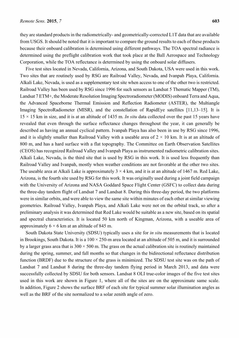
successfully collected by SDSU for both sensors. Landsat 8 OLI true-color images of the five test sites
used in this work are shown in Figure 1, where all of the sites are on the approximate same scale.
In addition, Figure 2 shows the surface BRF of each site for typical summer solar illumination angles as
well as the BRF of the site normalized to a solar zenith angle of zero.
Remote Sens. 2015, 7 604
SDSU
Figure 1. The test sites used to calibrate Landsat 8 OLI. All of the sites are on approximately
the same scale, and the true-color images are created using bands 2–4 of OLI. The arrows show
the general area(s) where surface reflectance measurements were made at each test site.
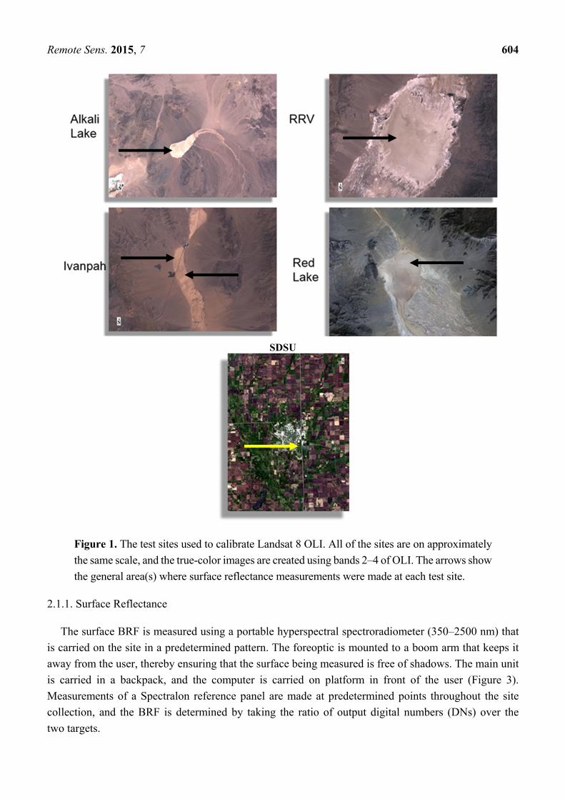
2.1.1. Surface Reflectance
The surface BRF is measured using a portable hyperspectral spectroradiometer (350–2500 nm) that
is carried on the site in a predetermined pattern. The foreoptic is mounted to a boom arm that keeps it
away from the user, thereby ensuring that the surface being measured is free of shadows. The main unit
is carried in a backpack, and the computer is carried on platform in front of the user (Figure 3).
Measurements of a Spectralon reference panel are made at predetermined points throughout the site
collection, and the BRF is determined by taking the ratio of output digital numbers (DNs) over the
two targets.

Remote Sens. 2015, 7 605
Figure 2. The hyperspectral surface BRF of the various test sites during typical summer
illumination angles (left). The results are obtained from portable spectroradiometers that are
carried across each site. The same results are shown with the solar zenith angle effect
removed (right). Noisy data due to atmospheric absorption, which creates a low SNR in the
portable spectrometers, have been removed for clarity.
Figure 3. Surface BRF collection at Ivanpah Playa (left) and the SDSU site (right).
The Spectralon field panels used by RSG and SDSU are routinely measured in RSG’s laboratory so
that the BRF is known as a function of angle and wavelength, and the panels are always used in the same
orientation in the field as well as when being measured in the laboratory [16–19]. The typical BRF for a
panel routinely used in the field is shown in Figure 4 for three wavelengths. The final BRF used in the
radiative transfer code is determined by spatially averaging over the test area and band averaging for
each of the bands of the sensor of interest. The size and orientation of the sampled area depends on the
architecture of the satellite sensor and the size of the site. In the case of a pushbroom sensor such as OLI,
the long side of the site is perpendicular to the spacecraft’s motion. In the case of a whiskbroom sensor
such as Landsat 7 ETM+, the long side of the site is oriented in the along-track direction of the satellite.

Remote Sens. 2015, 7 606
Figure 4. An example of the RSG results for the BRF of a Spectralon panel as a function of
angle at three wavelengths. There is minimal spread in the BRF as a function of wavelength,
which indicates that this panel has not yellowed due to ultraviolet (UV) exposure.
The size of the site is chosen to include a reasonable sample of the detectors. This is more practical
in the case of the 16 multispectral detectors of ETM+, but the large number of detectors in OLI means
that only a small sample of the complete detector package can be measured. Based on the heritage of
previous measurements for pushbroom sensors such as ASTER, the sites at Ivanpah Playa, Alkali Lake,
and Red Lake were chosen to be 120 × 300 m. The Railroad Valley site has semi-permanent tracks that
were established for the calibration of large-footprint sensors such as MODIS, so the site used for OLI
is a 90 × 500-m portion of the 1-km2 site. The collection area at the SDSU site is 100 × 250 m.
2.1.2. Atmospheric Measurements
Atmospheric measurements are made throughout the day with the goal of determining the atmospheric
transmission and radiance for each of the bands in the sensor under test during overpass. The automated
solar radiometer (ASR) is the primary atmospheric instrument used in the reflectance-based approach [20]
by both RSG and SDSU. An ASR tracks the sun throughout the day and measures the incoming solar
irradiance extinction due to atmospheric absorption and scattering. The ASR data are used to determine
the total atmospheric spectral optical depths, which are then broken down into subcomponents such as
the molecular, aerosol, ozone, and water vapor optical depths [21,22]. In the case of the desert sites used
by RSG, it is assumed that the aerosols can be modeled by a power law distribution, which means that
the Angstrom exponent can be used to define the aerosol size distribution. Columnar water vapor is
determined using a modified-Langley approach [23,24], and the columnar ozone amount from the Ozone
Monitoring Instrument (OMI) is used for this work. Ancillary data such as temperature and pressure are
measured using equipment that is brought to the site.
At the SDSU site, an ASR is used with a Langley analysis to derive instantaneous optical depth values.
The measurements from an Analytical Spectral Devices (ASD) spectrometer and a NIST-traceable
reflectance standard are combined to determine the surface reflectance of the field. These values along
with standard meteorological measurements and sensor view geometry are used as input into the
Remote Sens. 2015, 7 607
MODerate resolution atmospheric TRANsmission (MODTRAN) radiative transfer code. The initial
model is propagated from the sun through the atmosphere to ground level, and is used to predict:
(1) spectral radiance at the reflectance standard, (2) spectral radiance at the grass target, and (3) the
diffuse-to-global irradiance ratio of the sky. The results are compared to the radiance measurements
made with the ASD, and the diffuse-to-global ratio is compared to a Yankee Environmental Systems
shadow band radiometer. The comparison identifies any anomalies in the model predictions. If any are
identified, the model is updated and rerun until a model fit to reality is made. Once the model is matched
to the ground measurements, it is propagated to the top of the atmosphere. The data are then band
averaged using the RSRs of the sensor under test [25].
2.1.3. Top-of-Atmosphere Spectral Radiance and Reflectance
In general terms, the atmospheric and surface BRF measurements are used as inputs into the
MODTRAN radiative transfer code [26]. The in situ surface measurements are averaged so that BRF is
determined for the entire collection area at 1-nm intervals ranging from 350–2500 nm. The atmospheric
inputs include the solar and view geometries, the molecular optical depth, the aerosol optical depth,
columnar ozone, columnar water vapor, the Angstrom exponent, and the atmospheric index of refraction.
This work uses the ChKur (combined Chance and Kurucz) exoatmospheric solar irradiance, which is
distributed with MODTRAN 5. The output is the band-averaged TOA spectral radiance, which is also
converted to TOA reflectance for comparison with the two OLI products available from USGS.
The main advantage to using TOA reflectance is that the effects due to solar spectrum mismatch
are eliminated.
2.2. The Radiometric Calibration Test Site (RadCaTS) at Railroad Valley, Nevada
RadCaTS was developed by RSG to supplement the in situ data that are collected during routine field
campaigns. It is based on the reflectance-based approach, in that measurements of the atmosphere and
surface BRF are made during the time of interest. In the case of RadCaTS, the surface BRF
measurements are made using four ground-viewing radiometers (GVRs), and the atmospheric
measurements are made using a Cimel sun photometer, which is part of the global Aerosol Robotic
Network (AERONET) [27].
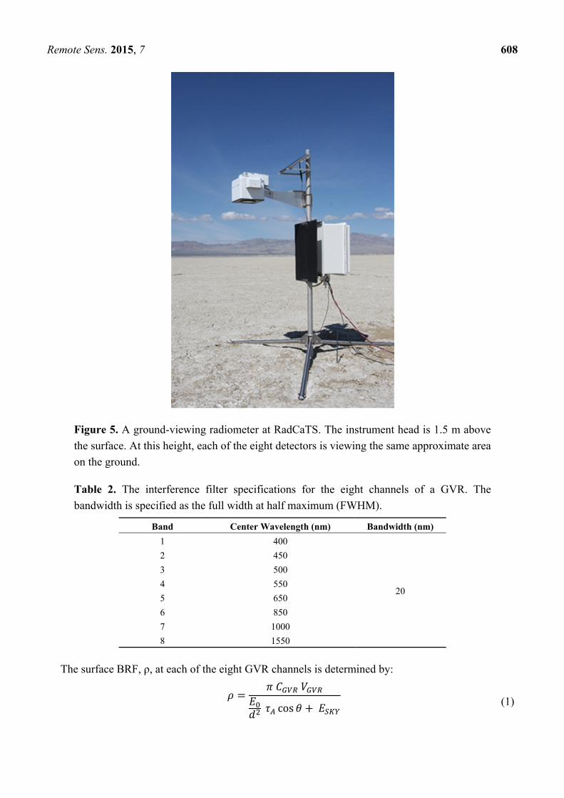
2.2.1. Surface Reflectance
The surface BRF measurement in RadCaTS is based on the reflectance-based approach, but it uses four
nadir-viewing radiometers that have been absolutely radiometrically calibrated, as opposed to taking the
ratio of the DNs measured over the ground to a reference panel (Figure 5). The current GVRs have eight
spectral channels that operate from 400 to 1550 nm (Table 2), and the spectral selection of each channel is
controlled using interference filters. The temperature of the critical electronics, including the focal plane,
is controlled using a thermo-electric (TE) cooler during daylight operation. Each GVR is an autonomous
standalone unit that is powered using a 12-V solar-charged system, and each unit includes its own data
logger [28,29]. The field of view is controlled using precise apertures, and there are no powered optics,
which is a concept similar to the ASRs that were developed at the University of Arizona.
Remote Sens. 2015, 7 608
Figure 5. A ground-viewing radiometer at RadCaTS. The instrument head is 1.5 m above
the surface. At this height, each of the eight detectors is viewing the same approximate area
on the ground.
Table 2. The interference filter specifications for the eight channels of a GVR. The
bandwidth is specified as the full width at half maximum (FWHM).
Band Center Wavelength (nm) Bandwidth (nm)
1 400
20
2 450
3 500
4 550
5 650
6 850
7 1000
8 1550
The surface BRF, ρ, at each of the eight GVR channels is determined by: = cos + (1)
Remote Sens. 2015, 7 609
where CGVR is the radiometric calibration coefficient of the GVR (W m−2 sr−1 µm−1)·V−1, VGVR is the
output voltage (V), E0 is the exoatmospheric spectral solar irradiance when the Earth-Sun distance is one
astronomical unit (AU) (W m−2·µm−1), d is the Earth-Sun distance (AU), τA is the direct solar beam
transmission (unitless), θ is the solar zenith angle, and Esky is the diffuse spectral sky irradiance
(W m−2·µm-1). AERONET Cimel sun photometer data are used as input into MODTRAN to determine
the direct solar beam transmission and the diffuse sky irradiance. The process of determining the
hyperspectral surface BRF for the time of interest is as follows:
1. The band-averaged surface BRF is determined for each channel of every GVR using Equation (1).
2. The band-averaged BRF of the entire 1-km2 site in each of the eight GVR channels is determined
by averaging the individual GVR measurements for each channel.
3. A reference spectra of hyperspectral data is chosen from a library of Railroad Valley BRF spectra.
4. The chosen reference spectra is fit to the average BRF using a least squares fit, which produces
a hyperspectral BRF for the date and time of interest.
The reference hyperspectral library is created from 12 years of in situ measurements of the 1-km2
area of Railroad Valley that is used to calibrate large-footprint sensors such as MODIS, MISR,
the Visible Infrared Imaging Radiometer Suite (VIIRS) and the Advanced Very High Resolution
Radiometer (AVHRR) [30–32]. The reference data are binned into monthly averages, which is
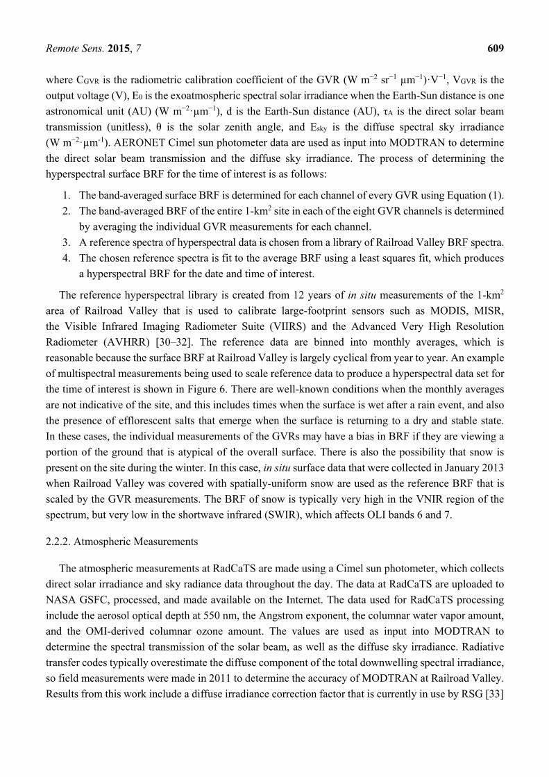
reasonable because the surface BRF at Railroad Valley is largely cyclical from year to year. An example
of multispectral measurements being used to scale reference data to produce a hyperspectral data set for
the time of interest is shown in Figure 6. There are well-known conditions when the monthly averages
are not indicative of the site, and this includes times when the surface is wet after a rain event, and also
the presence of efflorescent salts that emerge when the surface is returning to a dry and stable state.
In these cases, the individual measurements of the GVRs may have a bias in BRF if they are viewing a
portion of the ground that is atypical of the overall surface. There is also the possibility that snow is
present on the site during the winter. In this case, in situ surface data that were collected in January 2013
when Railroad Valley was covered with spatially-uniform snow are used as the reference BRF that is
scaled by the GVR measurements. The BRF of snow is typically very high in the VNIR region of the
spectrum, but very low in the shortwave infrared (SWIR), which affects OLI bands 6 and 7.
2.2.2. Atmospheric Measurements
The atmospheric measurements at RadCaTS are made using a Cimel sun photometer, which collects
direct solar irradiance and sky radiance data throughout the day. The data at RadCaTS are uploaded to
NASA GSFC, processed, and made available on the Internet. The data used for RadCaTS processing
include the aerosol optical depth at 550 nm, the Angstrom exponent, the columnar water vapor amount,
and the OMI-derived columnar ozone amount. The values are used as input into MODTRAN to
determine the spectral transmission of the solar beam, as well as the diffuse sky irradiance. Radiative
transfer codes typically overestimate the diffuse component of the total downwelling spectral irradiance,
so field measurements were made in 2011 to determine the accuracy of MODTRAN at Railroad Valley.
Results from this work include a diffuse irradiance correction factor that is currently in use by RSG [33]
Remote Sens. 2015, 7 610
Figure 6. An example showing how the multispectral surface BRF results from three GVRs
are used to scale reference hyperspectral BRF data. The reference data (blue) are shifted up
or down using the average of the multispectral GVR data (black points). Each of the points
at a given wavelength is from one of the three GVRs used during this specific date. The red
curve shows the resulting hyperspectral data that are used in the radiative transfer code for a
specific date and time of interest.
2.2.3. Top-of-Atmosphere Spectral Radiance and Reflectance
The output from MODTRAN for the RadCaTS data is similar to that of the in situ measurements.
The measurements from each GVR are averaged to create one hyperspectral BRF data set for the entire
1-km2 site for the date and time of interest. MODTRAN is used to process the hyperspectral surface BRF
and atmospheric measurements into band-averaged TOA quantities, which are then compared to the
imagery obtained from USGS.
The TOA spectral radiance, Lλ, is given by: = cos + (2)
where ρλ is the hyperspectral BRF determined using the GVRs, E0λ is the exoatmospheric spectral solar
irradiance when the Earth-Sun distance is one AU (W·m−2·µm−1), d is the Earth-Sun distance (AU),
τAλ is the direct solar beam transmission (unitless), θ is the solar zenith angle, and Esky λ is the diffuse
spectral sky irradiance (W·m−2·µm−1). The resulting hyperspectral TOA spectral radiance is band
averaged to each channel of the sensor under test (e.g., OLI or ETM+).
3. Data
3.1. Reflectance-Based Approach and Cross Calibration with ETM+
The ground-based data collection began after the completion of the check-out phase, which was thirty
days after launch. The test sites used were Railroad Valley, Nevada, Ivanpah Playa, California, Alkali
Lake, Nevada, and Red Lake, Arizona. In the early stages of the field collects, RSG was joined by
members of NASA GSFC, who were collecting data for OLI as well as for the calibration of the NASA
Remote Sens. 2015, 7 611
GSFC LiDAR Hyperspectral and Thermal (G-LiHT) airborne instruments [34]. The field team from
SDSU was concurrently collecting data at the SDSU field site. A summary of the conditions during the
field campaigns is shown in Tables 3 and 4, which also include the information for the tandem flight
period. RSG and GSFC were at Red Lake, Arizona, on 29 March 2013, and SDSU was at the SDSU site
on 30 March 2013. The ground-based measurements can be thought of as a transfer radiometer and SIS.
That is, the test sites act as stable radiometric sources during each overpass, which occurred within
several minutes of one another. The cross comparison is performed by comparing ETM+ and OLI to the
ground-based measurements.
Table 3. A summary of the in situ field campaign conditions for the University of Arizona
RSG (UA) and GSFC data collection.
Date (yyyy-
mm-dd)
2013-
03-19
2013-
03-24
2013-
03-29
2013-
04-20
2013-
04-29
2013-
10-15
2013-
11-14
2014-
02-04
2014-
03-08
2014-
05-09
Site (Team)
Railroad
Valley
(UA)
Ivanpah
Playa
(UA,
GSFC)
Red
Lake
(UA,
GSFC)
Railroad
Valley
(UA)
Ivanpah
Playa
(UA)
Red
Lake
(UA)
Railroad
Valley
(UA)
Red
Lake
(UA)
Red
Lake
(UA)
Railroad
Valley
(UA)
Collection
area (m)
90 ×
500
120 ×
300
120 ×
300
90 ×
500
120 ×
300
120 ×
300
90 ×
500
120 ×
300
120 ×
300
90 ×
500
Time (UTC) 18:19:54 18:16:29
18:05:34
(L7)
18:12:12
(L8)
18:22:47 18:17:26 18:11:03 18:22:47 18:10:33 18:09:55 18:20:38
Solar zenith
angle
(degrees)
44.0 40.0
38.9
(L7)
38.0
(L8)
32.0 27.7 46.6 58.9 56.3 46.3 27.1
Solar
azimuth
angle
(degrees)
146.4 142.8
140.0
(L7)
142.3
(L8)
141.4 133.7 159.7 162.1 151.2 145.6 135.2
Aerosol
Optical
Depth
(550 nm)
0.048 0.068 0.068 0.085 0.122 0.046 0.021 0.032 0.025 0.089
Ozone (DU) 298 296 306 309 323 286 326 333 311 356
Water vapor
(cm) 1.19 0.77 1.64 1.10 1.24 0.77 0.58 0.82 0.60 1.21
Temperature
(°C) 14.1 16.4 25.1 15.5 33.9 18.8 10.3 9.0 18.4 20.5
Pressure
(mb) 859.3 926.7 922.8 859.5 919.0 919.8 859.2 920.0 925.6 853.1
Remote Sens. 2015, 7 612
Table 3. Cont.
Date (yyyy-mm-
dd)
2013-
03-19
2013-
03-24
2013-
03-29
2013-
04-20
2013-
04-29
2013-
10-15
2013-
11-14
2014-
02-04
2014-
03-08
2014-
05-09
Satellite Information
View zenith
angle (degrees) 4.6 4.3
5.4 (L7)
2.7 (L8) 0.8 3.7 5.9 0.3 5.1 5.5 0.3
View azimuth
angle (degrees) 102.6 103.1
101.9
(L7)
100.7
(L8)
95.0 96.9 101.7 122.6 100.5 95.1 148.9
Table 4. A summary of the in situ field campaign conditions for the SDSU data collection.
Date
(yyyy-mm-dd) 2013-03-30 2013-06-10 2013-07-12 2013-08-13 2013-08-29 2013-09-30 2013-10-16
Site (Team)
SDSU Test
Site
(SDSU)
SDSU Test
Site
(SDSU)
SDSU Test
Site
(SDSU)
SDSU Test
Site
(SDSU)
SDSU Test
Site
(SDSU)
SDSU Test
Site
(SDSU)
SDSU Test
Site
(SDSU)
Collection area
(m) 100 × 250 100 × 250 100 × 250 100 × 250 100 × 250 100 × 250 100 × 250
Time (UTC)
17:07:14
(L7)
17:09:43
(L8)
17:13:23 17:13:22 17:13:23 17:13:25 17:13:15 17:13:14
Solar zenith angle
(degrees) 43.9 26.0 27.8 34.2 38.8 49.5 55.2
Solar azimuth
angle (degrees) 151.3 139.2 137.8 145.0 150.0 159.1 162.2
Aerosol Optical
Depth (550 nm) 0.158 0.060 0.183 0.195 0.067 0.016 0.077
Ozone (DU) 324 287 290 291 289 284 279
Water vapor (cm) 0.53 2.76 1.76 2.93 2.64 2.01 3.02
Temperature (°C) 7.2 18.9 27.8 21.7 31.0 22.5 8.9
Pressure (mb) 951.9 947.9 948.9 956.7 945.5 936.0 954.6
Satellite Information
View zenith angle
(degrees)
0.1 (L7)
5.0 (L8) 0.1 0.3 0.3 0.2 0.3 0.2
View azimuth
angle (degrees)
278.9 (L7)
278.9 (L8) 278.9 278.9 278.9 278.9 278.9 278.9
3.2. RadCaTS
A summary of the conditions at each of the successful RadCaTS collects is shown in Table 5, which
shows the solar and satellite viewing geometry as well as the key atmospheric components that are used
in MODTRAN. The collection dates should be similar to those of the in situ measurements made using
on-site personnel, but two dates in March and April 2013 were considered outliers due to spatial
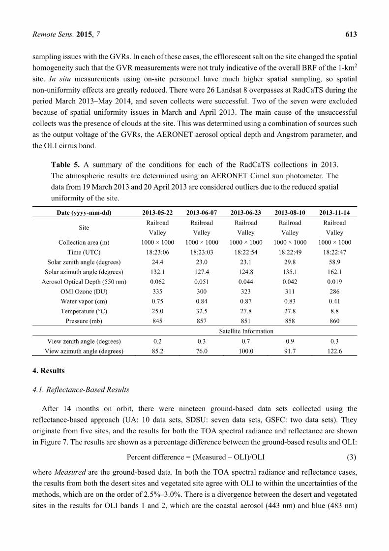
Remote Sens. 2015, 7 613
sampling issues with the GVRs. In each of these cases, the efflorescent salt on the site changed the spatial
homogeneity such that the GVR measurements were not truly indicative of the overall BRF of the 1-km2
site. In situ measurements using on-site personnel have much higher spatial sampling, so spatial
non-uniformity effects are greatly reduced. There were 26 Landsat 8 overpasses at RadCaTS during the
period March 2013–May 2014, and seven collects were successful. Two of the seven were excluded
because of spatial uniformity issues in March and April 2013. The main cause of the unsuccessful
collects was the presence of clouds at the site. This was determined using a combination of sources such
as the output voltage of the GVRs, the AERONET aerosol optical depth and Angstrom parameter, and
the OLI cirrus band.
Table 5. A summary of the conditions for each of the RadCaTS collections in 2013.
The atmospheric results are determined using an AERONET Cimel sun photometer. The
data from 19 March 2013 and 20 April 2013 are considered outliers due to the reduced spatial
uniformity of the site.
Date (yyyy-mm-dd) 2013-05-22 2013-06-07 2013-06-23 2013-08-10 2013-11-14
Site Railroad
Valley
Railroad
Valley
Railroad
Valley
Railroad
Valley
Railroad
Valley
Collection area (m) 1000 × 1000 1000 × 1000 1000 × 1000 1000 × 1000 1000 × 1000
Time (UTC) 18:23:06 18:23:03 18:22:54 18:22:49 18:22:47
Solar zenith angle (degrees) 24.4 23.0 23.1 29.8 58.9
Solar azimuth angle (degrees) 132.1 127.4 124.8 135.1 162.1
Aerosol Optical Depth (550 nm) 0.062 0.051 0.044 0.042 0.019
OMI Ozone (DU) 335 300 323 311 286
Water vapor (cm) 0.75 0.84 0.87 0.83 0.41
Temperature (°C) 25.0 32.5 27.8 27.8 8.8
Pressure (mb) 845 857 851 858 860
Satellite Information
View zenith angle (degrees) 0.2 0.3 0.7 0.9 0.3
View azimuth angle (degrees) 85.2 76.0 100.0 91.7 122.6
4. Results
4.1. Reflectance-Based Results
After 14 months on orbit, there were nineteen ground-based data sets collected using the
reflectance-based approach (UA: 10 data sets, SDSU: seven data sets, GSFC: two data sets). They
originate from five sites, and the results for both the TOA spectral radiance and reflectance are shown
in Figure 7. The results are shown as a percentage difference between the ground-based results and OLI:
Percent difference = (Measured – OLI)/OLI (3)
where Measured are the ground-based data. In both the TOA spectral radiance and reflectance cases,
the results from both the desert sites and vegetated site agree with OLI to within the uncertainties of the
methods, which are on the order of 2.5%–3.0%. There is a divergence between the desert and vegetated
sites in the results for OLI bands 1 and 2, which are the coastal aerosol (443 nm) and blue (483 nm)

Remote Sens. 2015, 7 614
bands. The source of this discrepancy is most likely due to a combination of very low surface reflectance
(Figure 2) and atmospheric effects, which play a larger role when the surface reflectance is less than 0.2.
At wavelengths greater than the vegetation red edge (700 nm), the surface reflectance of the vegetated
site increases rapidly to values similar to the desert sites. In the multispectral bands 3–7, the results
between the two types of sites and OLI agree to within the uncertainties of the methodology. In the
bottom row of Figure 7, the data from the three field teams are averaged into one final data set for both
TOA spectral radiance and reflectance. In the case of both TOA spectral radiance and reflectance,
OLI is generally in agreement with the ground-based results to within the design specifications (5% and
3%, respectively). The only band that is just out of specification is 7 (2.2 μm), which typically has a very
low signal at both the desert and vegetated sites.
TOA Spectral Radiance TOA Spectral Reflectance
TOA Spectral Radiance (average) TOA Spectral Reflectance (average)
Figure 7. A summary of in situ results from the University of Arizona RSG (UA), SDSU,
and GSFC for TOA spectral radiance (top left) and reflectance (top right) for Landsat 8 OLI.
The uncertainty bars are the 1σ standard deviation of the measurements by each team. Note
that band 9 (cirrus) is excluded from the results due to an extremely low SNR in the ground
measurements. The bottom row shows the results for TOA spectral radiance (bottom left)
and reflectance (bottom right) when the ground-based results from all three teams are
consolidated into one data set and then compared to OLI. The uncertainty bars in the average
graphs are the 1σ standard deviation of the average from all three teams.
Figures 8 and 9 show the temporal results of TOA spectral radiance and TOA reflectance,
respectively, for the fourteen-month duration of this work. The RSG data gap between Days Since
Launch (DSL) 77 and 246 was caused by poor weather conditions during the attempted field campaigns.
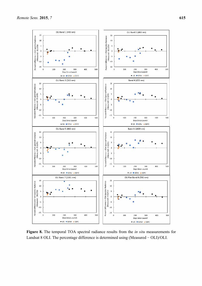
Remote Sens. 2015, 7 615
Figure 8. The temporal TOA spectral radiance results from the in situ measurements for
Landsat 8 OLI. The percentage difference is determined using (Measured − OLI)/OLI.

Remote Sens. 2015, 7 616
Figure 9. The temporal TOA spectral reflectance results from the in situ measurements for
Landsat 8 OLI. The percentage difference is determined using (Measured – OLI)/OLI.
Remote Sens. 2015, 7 617
The SDSU data gap after DSL 250 is due to winter conditions and the high probability of snow on
the site. The temporal results in both the TOA spectral radiance and reflectance cases do not show a
discernable trend in degradation in any of the channels at this time.
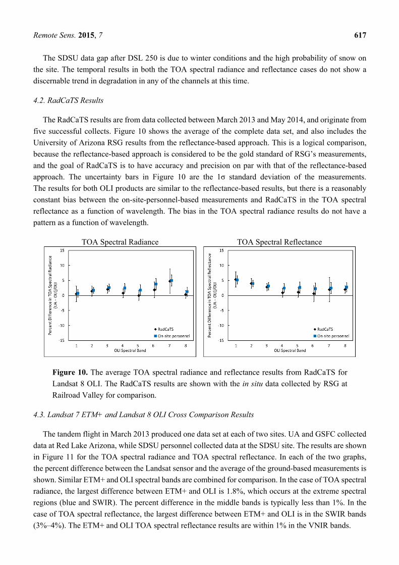
4.2. RadCaTS Results
The RadCaTS results are from data collected between March 2013 and May 2014, and originate from
five successful collects. Figure 10 shows the average of the complete data set, and also includes the
University of Arizona RSG results from the reflectance-based approach. This is a logical comparison,
because the reflectance-based approach is considered to be the gold standard of RSG’s measurements,
and the goal of RadCaTS is to have accuracy and precision on par with that of the reflectance-based
approach. The uncertainty bars in Figure 10 are the 1σ standard deviation of the measurements.
The results for both OLI products are similar to the reflectance-based results, but there is a reasonably
constant bias between the on-site-personnel-based measurements and RadCaTS in the TOA spectral
reflectance as a function of wavelength. The bias in the TOA spectral radiance results do not have a
pattern as a function of wavelength.
TOA Spectral Radiance TOA Spectral Reflectance
Figure 10. The average TOA spectral radiance and reflectance results from RadCaTS for
Landsat 8 OLI. The RadCaTS results are shown with the in situ data collected by RSG at
Railroad Valley for comparison.
4.3. Landsat 7 ETM+ and Landsat 8 OLI Cross Comparison Results
The tandem flight in March 2013 produced one data set at each of two sites. UA and GSFC collected
data at Red Lake Arizona, while SDSU personnel collected data at the SDSU site. The results are shown
in Figure 11 for the TOA spectral radiance and TOA spectral reflectance. In each of the two graphs,
the percent difference between the Landsat sensor and the average of the ground-based measurements is
shown. Similar ETM+ and OLI spectral bands are combined for comparison. In the case of TOA spectral
radiance, the largest difference between ETM+ and OLI is 1.8%, which occurs at the extreme spectral
regions (blue and SWIR). The percent difference in the middle bands is typically less than 1%. In the
case of TOA spectral reflectance, the largest difference between ETM+ and OLI is in the SWIR bands
(3%–4%). The ETM+ and OLI TOA spectral reflectance results are within 1% in the VNIR bands.
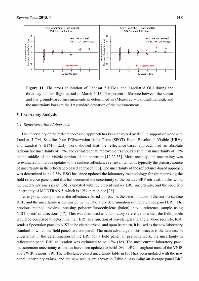
Remote Sens. 2015, 7 618
Figure 11. The cross calibration of Landsat 7 ETM+ and Landsat 8 OLI during the
three-day tandem flight period in March 2013. The percent difference between the sensor
and the ground-based measurements is determined as (Measured – Landsat)/Landsat, and
the uncertainty bars are the 1σ standard deviation of the measurements.
5. Uncertainty Analysis
5.1. Reflectance-Based Approach
The uncertainty of the reflectance-based approach has been analyzed by RSG in support of work with
Landsat 5 TM, Satellite Pour l’Observation de la Terre (SPOT) Haute Resolution Visible (HRV),
and Landsat 7 ETM+. Early work showed that the reflectance-based approach had an absolute
radiometric uncertainty of ±5%, and estimated that improvements should result in an uncertainty of ±3%
in the middle of the visible portion of the spectrum [12,22,35]. More recently, the uncertainty was
re-evaluated to include updates to the surface reflectance retrieval, which is typically the primary source
of uncertainty in the reflectance-based approach [36]. The uncertainty of the reflectance-based approach
was determined to be 2.5%. RSG has since updated the laboratory methodology for characterizing the
field reference panels, and this has decreased the uncertainty of the surface BRF retrieval. In this work,
the uncertainty analysis in [36] is updated with the current surface BRF uncertainty, and the specified
uncertainty of MODTRAN 5, which is ±2% in radiance [26].
An important component in the reflectance-based approach is the determination of the test site surface
BRF, and the uncertainty is dominated by the laboratory determination of the reference panel BRF. The
previous method involved pressing polytetrafluoroethylene (halon) into a reference sample using
NIST-specified directions [17]. This was then used as a laboratory reference to which the field panels
would be compared to determine their BRF as a function of wavelength and angle. More recently, RSG
sends a Spectralon panel to NIST to be characterized, and upon its return, it is used as the new laboratory
standard to which the field panels are compared. The main advantage to this process is the decrease in
uncertainty in the determination of the BRF for a field panel. In previous work, the uncertainty in
reflectance panel BRF calibration was estimated to be ±2% (1σ). The most current laboratory panel
measurement uncertainty estimates have been updated to be ±1.0%–1.4% throughout most of the VNIR
and SWIR regions [19]. The reflectance-based uncertainty table in [36] has been updated with the new
panel uncertainty values, and the new results are shown in Table 6. Assuming an average panel BRF
Remote Sens. 2015, 7 619
measurement uncertainty of ±1.3% over the VNIR and SWIR, the current uncertainty in the TOA
spectral radiance is ±2.6% in the middle of the visible spectral region. The value of “---” is shown in the
absorption computation for the 2005 analysis because it addressed the fact that wavelengths could be
chosen where there is a negligible effect on the retrieved TOA spectral radiance due to water vapor or
ozone. The same value of “---” is shown in the non-lambertian surface column, and it is justified by
previous research that has shown that the non-lambertian nature of Railroad Valley is negligible in the
determination of TOA spectral radiance for near-nadir view angles and typical aerosol conditions.
Table 6. The uncertainty of the reflectance-based approach, which includes updated values
for the laboratory calibration of Spectralon reference panels. The table is based on earlier
results presented in [35] and is valid for clear-sky conditions in the middle of the visible
spectral region.
Source of Uncertainty Source TOA Spectral Radiance
Ground reflectance measurement 1.6%
Reference panel calibration (BRF) 1.3%
Site measurement errors 1.0%
Optical depth measurements 0.5% <0.1%
Extinction optical depth 0.5%
Absorption computations ---
Column ozone (OMI) 3.0%
Column water vapor 5.0%
Choice of aerosol complex index 100% 0.5%
Choice of aerosol size distribution 0.3%
Junge parameter 0.3%
Non-lambertian surface 10% ---
Other
Non-polarization vs. polarization 0.1%
Inherent accuracy of MODTRAN 5 2.0%
Uncertainty in solar zenith angle 0.2%
Total RSS uncertainty 2.6%
5.2. RadCaTS
The RadCaTS methodology is modeled on the reflectance-based approach, and the determination of
surface BRF is also the primary influence in the uncertainty of TOA quantities. In the RadCaTS processing
scheme, the surface BRF, ρ, is determined using Equation (1). The uncertainty, Δρ, is given by:
Δρ = ΔC + ΔV + ΔE + Δτ + Δ + ΔE (4)
where ΔCGVR is the uncertainty in the GVR radiometric calibration coefficient, ΔVGVR is the uncertainty
in the output voltage, ΔE0 is the uncertainty in the exoatmospheric solar irradiance, ΔτA is the uncertainty
in the atmospheric transmission, Δθ is the uncertainty of the solar zenith angle, and ΔESKY is the
uncertainty in the diffuse sky irradiance. Similarly, the uncertainty in TOA spectral radiance, ΔL,
determined in Equation (2) is:
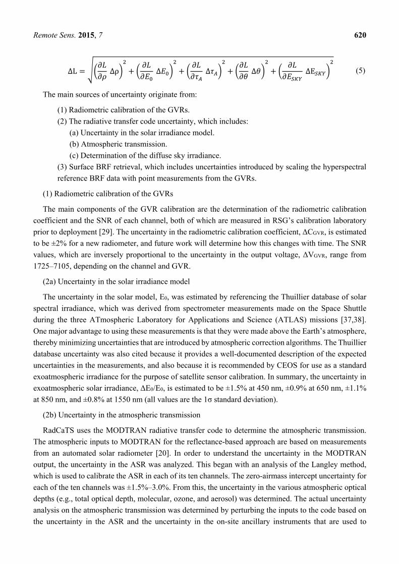
Remote Sens. 2015, 7 620
ΔL = ∂ Δρ + ∂ Δ + Δ + Δ + ∂ ΔE (5)
The main sources of uncertainty originate from:
(1) Radiometric calibration of the GVRs.
(2) The radiative transfer code uncertainty, which includes:
(a) Uncertainty in the solar irradiance model.
(b) Atmospheric transmission.
(c) Determination of the diffuse sky irradiance.
(3) Surface BRF retrieval, which includes uncertainties introduced by scaling the hyperspectral
reference BRF data with point measurements from the GVRs.
(1) Radiometric calibration of the GVRs
The main components of the GVR calibration are the determination of the radiometric calibration
coefficient and the SNR of each channel, both of which are measured in RSG’s calibration laboratory
prior to deployment [29]. The uncertainty in the radiometric calibration coefficient, ΔCGVR, is estimated
to be ±2% for a new radiometer, and future work will determine how this changes with time. The SNR
values, which are inversely proportional to the uncertainty in the output voltage, ΔVGVR, range from
1725–7105, depending on the channel and GVR.
(2a) Uncertainty in the solar irradiance model
The uncertainty in the solar model, E0, was estimated by referencing the Thuillier database of solar
spectral irradiance, which was derived from spectrometer measurements made on the Space Shuttle
during the three ATmospheric Laboratory for Applications and Science (ATLAS) missions [37,38].
One major advantage to using these measurements is that they were made above the Earth’s atmosphere,
thereby minimizing uncertainties that are introduced by atmospheric correction algorithms. The Thuillier
database uncertainty was also cited because it provides a well-documented description of the expected
uncertainties in the measurements, and also because it is recommended by CEOS for use as a standard
exoatmospheric irradiance for the purpose of satellite sensor calibration. In summary, the uncertainty in
exoatmospheric solar irradiance, ΔE0/E0, is estimated to be ±1.5% at 450 nm, ±0.9% at 650 nm, ±1.1%
at 850 nm, and ±0.8% at 1550 nm (all values are the 1σ standard deviation).
(2b) Uncertainty in the atmospheric transmission
RadCaTS uses the MODTRAN radiative transfer code to determine the atmospheric transmission.
The atmospheric inputs to MODTRAN for the reflectance-based approach are based on measurements
from an automated solar radiometer [20]. In order to understand the uncertainty in the MODTRAN
output, the uncertainty in the ASR was analyzed. This began with an analysis of the Langley method,
which is used to calibrate the ASR in each of its ten channels. The zero-airmass intercept uncertainty for
each of the ten channels was ±1.5%–3.0%. From this, the uncertainty in the various atmospheric optical
depths (e.g., total optical depth, molecular, ozone, and aerosol) was determined. The actual uncertainty
analysis on the atmospheric transmission was determined by perturbing the inputs to the code based on
the uncertainty in the ASR and the uncertainty in the on-site ancillary instruments that are used to
Remote Sens. 2015, 7 621
measure temperature and pressure, for example. The ozone input is determined using OMI data, which
are stated to have an uncertainty of ±3% [39]. The results from the study showed that the uncertainty in
atmospheric transmission, ΔτA, ranged from ±1.1% in the blue region of the spectrum down to ±0.3% in
the SWIR region of the spectrum.
RadCaTS uses a Cimel sun photometer to perform atmospheric measurements. The instrument is
routinely calibrated at NASA GSFC, and the uncertainty in aerosol optical depth during clear-sky
conditions is stated to be ±0.010 for wavelengths greater than 440 nm, and ±0.020 for wavelengths less
than 440 nm [27]. An analysis of the ASRs indicate that the uncertainty of the retrieved aerosol optical
depth at 550 nm is ±0.006 on average for typical clear-sky conditions. Even though the uncertainty in
the aerosol optical depth that is determined using a Cimel is slightly larger than that from an ASR,
this work assumes that the uncertainty in atmospheric transmittance is of the same order of magnitude.
Further analysis is underway to compare the atmospheric properties determined using the Cimel and
ASR, and their effect on the TOA spectral radiance uncertainty.
(2c) Uncertainty in the diffuse sky irradiance
The diffuse sky irradiance, ESKY, is perhaps one of the more difficult quantities to determine
accurately using radiative transfer codes. In 2011, RSG personnel directly measured ESKY during an
experiment to determine to accuracy of the MODTRAN 5.2 output under typical clear-sky conditions at
Railroad Valley [33]. A hyperspectral spectroradiometer was used to measure the surface reflectance at
the same time as a GVR. It was found that the MODTRAN prediction of ESKY at Railroad Valley was
as much as 50% higher in the VNIR than measurements made using a calibrated spectroradiometer. This
discrepancy can change the surface reflectance retrieval by as much as 10%, most notably in the blue
region where the ratio of diffuse-to-global solar irradiance is greatest. An ESKY correction factor that
accounted for the large difference between MODTRAN and the measured values was created and is
currently in use. After the correction is applied, the uncertainty in ESKY is estimated to be ±5% at this
time. The correction factor is currently applicable to conditions that are similar to those when the
measurements were made, that is, low aerosol optical depth (δ550 nm < 0.10) and cloud free. Additional
field work will be completed in the future to further understand and enhance the correction factor
for ESKY.
(3) Uncertainty in surface BRF retrieval
The four GVRs at RadCaTS are effectively making point measurements of a 1-km2 region.
Two studies were undertaken to determine the accuracy of this configuration, and to see how well the
results compare to the typical manned vicarious calibration method, where a portable spectroradiometer
is carried 4.8 km throughout the site [40,41]. Results from both of these studies indicate that because of
Railroad Valley’s homogeneity, four radiometers are adequate to sample the 1-km2 site to within ±2%
of the average value. In terms of accuracy, the surface reflectance determined using four RadCaTS GVRs
agreed to within ±1% of those made using traditional portable spectroradiometers.
The overall uncertainty in the surface BRF retrieval for RadCaTS consists of two parts: the inherent
uncertainty of an individual GVR measurement, and the uncertainty introduced by fitting the
hyperspectral BRF reference data to the BRF determined by the GVRs. That is, the resulting
hyperspectral BRF data will differ slightly from the average of the GVR measurements for a given date

Remote Sens. 2015, 7 622
and time (Figure 6). The uncertainty created by shifting the hyperspectral reference data was determined
by measuring the magnitude of the scaling effect for twenty three dates in 2013 when RadCaTS was in
use. The scaling factor was analyzed at 18:30 and 20:50 UTC, which is approximately symmetric in time
around solar noon. The analysis was also performed to determine if there is a morning-afternoon bias since
most of the in situ reference BRF data were collected during morning overpasses (e.g., Terra MODIS).
Table 7 shows the overall uncertainty in BRF, which is the RSS of the two individual uncertainties.
Table 7. The RadCaTS surface BRF uncertainty (1σ) for four of the GVR spectral bands for
typical clear-sky conditions and a solar zenith angle of 45°.
Source of Uncertainty
Surface BRF Uncertainty
GVR Band
450 nm 650 nm 850 nm 1550 nm
Individual GVR measurement 2.7% 2.4% 2.5% 2.2%
Scaling hyperspectral reference data 2.6% 1.7% 2.8% 3.3%
Total BRF uncertainty 3.7% 2.9% 3.8% 4.0%
RadCaTS Uncertainty Results
The uncertainty analysis results assume that there are clear-sky conditions, and the solar zenith angle
is 45°, which was chosen as a representative value for the overpass times of sun-synchronous
Earth-observing sensors at Railroad Valley. When extremes in solar zenith angle are used (e.g., 15°
and 60°), the uncertainty in surface BRF and TOA spectral radiance varies by ±0.5%. Typical
spectrally-dependent values for E0, τA, and ESKY were used in this analysis.
When the results of the individual inputs are used in (5), the uncertainty in the TOA spectral radiance
determined using RadCaTS is shown in Table 8 for four of the eight GVR bands. The overall uncertainty
is generally dominated by the uncertainty in the BRF retrieval, but ESKY plays a greater role in the blue
end of the spectrum.
Table 8. The RadCaTS TOA spectral radiance uncertainty (1σ) for four of the GVR spectral
channels for typical clear-sky conditions and a solar zenith angle of 45°.
RadCaTS TOA Spectral Radiance Uncertainty
GVR Band
450 nm 650 nm 850 nm 1550 nm
4.1% 3.1% 4.1% 4.1%
6. Conclusions
The results from an extensive campaign of ground-based field measurements during the first year of
operation have indicated that the Landsat 8 OLI instrument is performing well, and it has remained stable
throughout this period. The ground-based data collected for this work were compared to the L1T imagery
that are available from USGS through Earth Explorer. When all of the reflectance-based field data are
averaged together, there is agreement with OLI in each spectral band to within the design specifications
for TOA spectral radiance (5%), and TOA spectral reflectance (3%), except for band 7, which is slightly
higher in both cases. The temporal results have not shown an appreciable pattern of degradation in the
Remote Sens. 2015, 7 623
OLI instrument. The results from the automated RadCaTS facility at Railroad Valley have shown results
similar to those obtained by ground personnel, having slightly better agreement with OLI than in situ
measurements made by on-site personnel at Railroad Valley. The number of RadCaTS data sets was
smaller than one would expect throughout the year, and this was mainly due to the abnormally high
number of dates with poor weather conditions throughout the year.
Ground-based calibration work will continue using on-site personnel from the University of Arizona
and South Dakota State University. In addition, RadCaTS will also be used to monitor OLI throughout
its mission lifetime. The excellent radiometric performance and stability of OLI will assist vicarious
calibration teams to refine their methodologies and field collection techniques, which includes the
automated RadCaTS facility.
Acknowledgements
The authors would like to thank the Bureau of Land Management (BLM) Tonopah, Nevada, office
for their assistance and permission in using Railroad Valley, and the BLM, Needles, California, office
for their assistance in using Ivanpah Playa. The authors would also like to thank the reviewers of this
paper for their comments and suggestions. This research was supported by NASA grants NNX11AG28G
and NNX09AH23A, and USGS grants G08AC00031 and G14AC00371.
Author Contributions
All of the authors were involved various aspects of the data collection and/or analysis during the
period of this work. Jeff Czapla-Myers and Nikolaus Anderson were involved in the in situ collection
and analysis of field data, which included simultaneous field work with Kurt Thome and Joel McCorkel,
who provided the GSFC results. Stuart Biggar was part of the preflight calibration team that made
measurements at Ball Aerospace and NIST. Larry Leigh and David Aaron were involved in the SDSU
field campaigns, and provided the SDSU results for this paper. Dennis Helder and Nischal Mishra
provided expertise in the analysis of the field data.
Conflicts of Interest
The authors declare no conflict of interest.
References
1. Reuter, D.; Richardson, C.; Irons, J.; Allen, R.; Anderson, M.; Budinoff, J.; Casto, G.; Coltharp, C.;
Finneran, P.; Forsbacka, B.; et al. The Thermal Infrared Sensor on the Landsat Data Continuity
Mission. In Proceedings of 2010 IEEE International Geoscience and Remote Sensing Symposium
(IGARSS), Honolulu, HI, USA, 25–30 July 2010.
2. Reuter, D.; Richardson, C.; Pellerano, F.; Irons, J.; Allen, R.; Anderson, M.; Jhabvala, M.;
Lunsford, A.; Montanaro, M.; Smith, R.; et al. The Thermal Infrared Sensor (TIRS) on Landsat 8:
Design overview and pre-launch characterization. Remote Sens. 2015, 7, in press.
3. Ungar, S.G.; Pearlman, J.S.; Mendenhall, J.A.; Reuter, D. Overview of the Earth Observing One
(EO-1) mission. IEEE Trans. Geosci. Remote Sens. 2003, 41, 1149–1159.
Remote Sens. 2015, 7 624
4. Irons, J.R.; Dwyer, J.L.; Barsi, J.A., The next Landsat satellite: The Landsat Data Continuity
Mission. Remote Sens. Environ. 2012, 122, 11–21.
5. Markham, B.; Barsi, J.; Kvaran, G.; Ong, L.; Kaita, E.; Biggar, S.; Czapla-Myers, J.; Mishra, N.;
Helder, D. Landsat-8 operational land imager radiometric calibration and stability. Remote Sens.
2014, 6, 12275–12308.
6. Kuester, M.A.; Czapla-Myers, J.; Kaptchen, P.; Good, W.; Lin, T.; To, R.; Biggar, S.; Thome, K.
Development of a heliostat facility for solar-radiation-based calibration of earth observing sensors.
In Proceedings of Earth Observing Systems XIII, San Diego, CA, USA, 28 August 2008.
7. Czapla-Myers, J.; Thome, K.; Anderson, N.; McCorkel, J.; Leisso, N.; Good, W.; Collins, S.
Transmittance measurement of a heliostat facility used in the preflight radiometric calibration of
Earth-observing sensors. In Proceedings of SPIE Optics and Photonics 2009, San Diego, CA, USA,
2–6 August 2009.
8. Knight, E.; Kvaran, G. Landsat-8 operation land imager design, characterization and performance.
Remote Sens. 2014, 6, 10286–10305.
9. Slater, P.N.; Biggar, S.F.; Holm, R.G.; Jackson, R.D.; Mao, Y.; Moran, M.S.; Palmer, J.M.;
Yuan, B. Reflectance- and radiance-based methods for the in-flight absolute calibration of
multispectral sensors. Remote Sens. Environ. 1987, 22, 11–37.
10. Teillet, P.M.; Slater, P.N.; Ding, Y.; Santer, R.P.; Jackson, R.D.; Moran, M.S. Three methods for
the absolute calibration of the NOAA AVHRR sensors in-flight. Remote Sens. Environ. 1990, 31,
105–120.
11. Thome, K.J.; Crowther, B.G.; Biggar, S.F. Reflectance- and irradiance-based calibration of Landsat
5 thematic mapper. Can. J. Remote Sens. 1997, 23, 309–317.
12. Thome, K.J. Absolute radiometric calibration of Landsat 7 ETM+ using the reflectance-based
method. Remote Sens. Environ. 2001, 78, 27–38.
13. Thome, K.J.; Biggar, S.F.; Choi, H.J. Vicarious calibration of Terra ASTER, MISR, and MODIS.
In Proceedings of Earth Observing Systems IX, Denver, CO, USA, 26 October 2004.
14. Thome, K.J.; Arai, K.; Tsuchida, S.; Biggar, S.F. Vicarious calibration of ASTER via the
reflectance-based approach. IEEE Trans. Geosci. Remote Sens. 2008, 46, 3285–3295.
15. Naughton, D.; Brunn, A.; Czapla-Myers, J.; Douglass, S.; Thiele, M.; Weichelt, H.; Oxfort, M.
Absolute radiometric calibration of the RapidEye Multi-Spectral Imager using the reflectance based
vicarious calibration method. J. Appl. Remote Sens. 2011, 5, doi:10.1117/1.3613950.
16. Jackson, R.D.; Moran, M.S.; Slater, P.N.; Biggar, S.F. Field calibration of reference reflectance
panels. Remote Sens. Environ. 1987, 22, 145–158.
17. Biggar, S.F.; Labed, J.F.; Santer, R.P.; Slater, P.N.; Jackson, R.D.; Moran, M.S. Laboratory
calibration of field reflectance panels. In Proceedings of Recent Advances in Sensors, Radiometry,
and Data Processing for Remote Sensing, Orlando, FL, USA, 6–8 April 1988.
18. Anderson, N.J.; Biggar, S.F.; Burkhart, C.; Thome, K.J.; Mavko, M.E. Bi-directional calibration
results for the cleaning of spectralon reference panels. In Proceedings of Earth Observing Systems
VII, Seattle, WA, USA, 24 September 2002.
19. Helder, D.; Thome, K.; Aaron, D.; Leigh, L.; Czapla-Myers, J.; Leisso, N.; Biggar, S.; Anderson, N.
Recent surface reflectance measurement campaigns with emphasis on best practices, SI traceability
and uncertainty estimation. Metrologia 2012, 49, doi:10.1088/0026-1394/49/2/S21.
Remote Sens. 2015, 7 625
20. Ehsani, A.R.; Reagan, J.A.; Erxleben, W.H. Design and performance analysis of an automated
10-channel solar radiometer instrument. J. Atmos. Oceanic Technol. 1998, 15, 697–707.
21. Biggar, S.F.; Gellman, D.I.; Slater, P.N. Improved evaluation of optical depth components from
langley plot data. Remote Sens. Environ. 1990, 32, 91–101.
22. Biggar, S.F.; Slater, P.N.; Gellman, D.I. Uncertainties in the in-flight calibration of sensors with
reference to measured ground sites in the 0.4–1.1 μm range. Remote Sens. Environ. 1994, 48,
245–252.
23. Reagan, J.A.; Thome, K.J.; Herman, B.M. A Simple Instrument and Technique for Measuring
Columnar Water Vapor via Near-IR Differential Solar Transmission Measurments. In Proceedings
of Geoscience and Remote Sensing Symposium, 1991. IGARSS’91. Remote Sensing: Global
Monitoring for Earth Management, International, Espo, Finland, 3–6 Jun 1991.
24. Thome, K.J.; Smith, M.W.; Palmer, J.M.; Reagan, J.A. Three-channel solar radiometer for the
determination of atmospheric columnar water vapor. Appl. Opt. 1994, 33, 5811–5819.
25. Thome, K.J.; Helder, D.L.; Aaron, D.; Dewald, J.D. Landsat-5 TM and Landsat-7 ETM+ absolute
radiometric calibration using the reflectance-based method. IEEE Trans. Geosci. Remote Sens.
2004, 42, 2777–2785.
26. Berk, A.; Anderson, G.P.; Acharya, P.K.; Shettle, E.P. MODTRAN 5.2.1 User’s Manual; Spectral
Sciences Inc., Air Force Research Laboratory: Burlington, MA, USA and Hanscom AFB, MA,
USA, 2011.
27. Holben, B.N.; Eck, T.F.; Slutsker, I.; Tanré, D.; Buis, J.P.; Setzer, A.; Vermote, E.; Reagan, J.A.;
Kaufman, Y.J.; Nakajima, T.; Lavenu, F.; Janjowiak, I.; Smirnov, A. AERONET—A federated
instrument network and data archive for aerosol characterization. Remote Sens. Environ. 1998, 66,
1–16.
28. Anderson, N.J.; Czapla-Myers, J.S. Ground viewing radiometer characterization, implementation
and calibration applications: A summary after two years of field deployment. In Proceedings of
Earth Observing Systems XVIII, San Diego, CA, USA, 23 September 2013.
29. Anderson, N.; Czapla-Myers, J.; Leisso, N.; Biggar, S.; Burkhart, C.; Kingston, R.; Thome, K.
Design and calibration of field deployable ground-viewing radiometers. Appl. Opt. 2013, 52,
231–240.
30. Thome, K.; Smith, N.; Scott, K. Vicarious calibration of MODIS using Railroad Valley Playa.
In Proceedings of International Geoscience and Remote Sensing Symposium 2001 (IGARSS),
Sydney, Australia, 9–13 July 2001.
31. Thome, K.; D’Amico, J.; Hugon, C. Intercomparison of Terra ASTER, MISR, and MODIS, and
Landsat-7 ETM+. In Proceedings of IEEE International Conference on Geoscience and Remote
Sensing Symposium, IGARSS 2006, Denver, CO, USA, 31 July–4 August 2006.
32. Czapla-Myers, J.S.; Thome, K.J.; Leisso, N.P. Calibration of AVHRR sensors using the
reflectance-based method. In Proceedings of Atmospheric and Environmental Remote Sensing Data
Processing and Utilization III: Readiness for GEOSS, San Diego, CA, USA, 24 September 2007.
33. Leisso, N.; Czapla-Myers, J. Comparison of diffuse sky irradiance calculation methods and effect
on surface reflectance retrieval from an automated radiometric calibration test site. In Proceedings
of Earth Observing Systems XVI, San Diego, CA, USA, 14 September 2011.

Remote Sens. 2015, 7 626
34. Cook, B.D.; Corp, L.A.; Nelson, R.F.; Middleton, E.M.; Morton, D.C.; McCorkel, J.T.;
Masek, J.G.; Ranson, K.J.; Vuong, L.; Montesano, P.M. NASA Goddard’s LiDAR, Hyperspectral
and Thermal (G-LiHT) airborne imager. Remote Sens. 2013, 5, 4045–4066.
35. Slater, P.N.; Biggar, S.F.; Thome, K.J.; Gellman, D.I.; Spyak, P.R. Vicarious radiometric
calibrations of EOS sensors. J. Atmos. Oceanic Technol. 1996, 13, 349–359.
36. Thome, K.; Cattrall, C.; D’Amico, J.; Geis, J. Ground-reference calibration results for Landsat-7
ETM+. In Proceedings of Earth Observing Systems X, San Diego, CA, USA, 7 September 2005.
37. Thuillier, G.; Hersé, M.; Simon, P.; Labs, D.; Mandel, H.; Gillotay, D.; Foujols, T. The visible solar
spectral irradiance from 350 to 850 nm as measured by the solspec spectrometer during the Atlas I
Mission. In Solar Electromagnetic Radiation Study for Solar Cycle 22; Pap, J.M., Fröhlich, C.,
Ulrich, R.K., Eds.; Springer: Berlin, Germany, 1998; pp. 41–61.
38. Thuillier, G.; Hersé, M.; Labs, D.; Foujols, T.; Peetermans, W.; Gillotay, D.; Simon, P.C.; Mandel, H.
The solar spectral irradiance from 200 to 2400 nm as measured by the SOLSPEC spectrometer from
the Atlas and Eureca Missions. Sol. Phys. 2003, 214, 1–22.
39. Bhartia, P.K. OMI algorithm theoretical basis document. Volume II. OMI Ozone Products.
Available online: eospso.gsfc.nasa.gov/sites/default/files/atbd/ATBD-OMI-02.pdf (accessed on 1
August 2014).
40. Czapla-Myers, J.S.; Thome, K.J.; Buchanan, J.H. Implication of spatial uniformity on vicarious
calibration using automated test sites. In Proceedings of Earth Observing Systems XII, San Diego,
CA, USA, 27 September 2007.
41. Czapla-Myers, J.S.; Thome, K.J.; Cocilovo, B.R.; McCorkel, J.T.; Buchanan, J.H. Temporal,
spectral, and spatial study of the automated vicarious calibration test site at Railroad Valley,
Nevada. In Proceedings of Earth Observing Systems XIII, San Diego, CA, USA, 20 August 2008.
© 2015 by the authors; licensee MDPI, Basel, Switzerland. This article is an open access article
distributed under the terms and conditions of the Creative Commons Attribution license
(http://creativecommons.org/licenses/by/4.0/).