The Great Wall of Debt:

The Cross Section of Chinese Local

Government Credit Spreads∗

Andrew Ang† Jennie Bai‡ Hao Zhou §

September 4, 2015

JEL Classification: D73, G12, G14, G28, H74.

Key Words: chengtou bond, corruption, real estate, local government financing vehicle

(LGFV), government guarantee, systemic risk.

∗We thank Jennifer Carpenter, Darrell Duffie, Arvind Krishnamurthy, Stijn Van Nieuwerburgh, andseminar participants at New York University, Stanford GSB, Georgetown, George Washington University,the IMF, the World Bank, Tsinghua University, Federal Reserve Board, and the Brookings Institution,for helpful comments and suggestions. We also thank Angsheng Gu and Yichen Li for excellent researchassistance. An animated graph of chengtou bond issuance can be found at http://www.columbia.edu/

~aa610/chinamuni.html†Ann F. Kaplan Professor of Business, Columbia Business School, 3022 Broadway, 413 Uris, New York,

NY 10027. Phone: (212) 854-9154, Email: aa610@columbia.edu.‡Assistant Professor of Finance, McDonough School of Business, Georgetown University, Washington,

D.C. 20057. Phone: (202) 687-5695, Email: Jennie.Bai@georgetown.edu (corresponding author).§Unigroup Chair Professor, PBC School of Finance, Tsinghua University. Phone: +86-10-62790655,

Email: zhouh@pbcsf.tsinghua.edu.cn.

The Great Wall of Debt:

The Cross Section of Chinese Local

Government Credit Spreads

Abstract

Chinese chengtou bond, although implicitly guaranteed by the central government,

show sharp cross-sectional variations in excess yields, with respect to local economic

fundamentals—GDP growth, fiscal surplus, and real estate price. Opposite to what we

have learned from the U.S. municipal market, factors reflecting China’s aggregate credit

risk and monetary policy are actually priced in the cross section. Furthermore, counter-

intuitively, chengtou bond yields are higher for provinces with higher GDP growth and

fiscal surplus, which is only sensible when there is severe credit rationing. Reflecting

the nature of their collateral, positive real estate variables are important drivers of

higher chengtou bond prices; while market liquidity is lowing chengtou bond prices—

consistent with reaching-for-yield story. We find a significantly positive relationship

between chengtou bond yields and an index of local government corruption, with the

influence of corruption likely working through the real estate channel.

1 Introduction

Chengtou bonds are financial obligations of Chinese local governments. Capital raised

through the chengtou bond market finances, to a large extent, the tremendous growth in the

infrastructure projects in China—ranging from megaprojects like the $2.4 billion Shanghai

Tower (the second tallest building in the world) to the housing estates sprouting in many

cities. From 2008 to 2014, the chengtou bond market increases by 85% per year, and as

of December 2014, there are RMB 4.95 trillion ($0.82 trillion) chengtou bonds outstanding.

The brisk increase in chengtou liabilities goes hand-in-hand with the growth of total debt

in China, which increases from 130% of GDP in 2008 to over 200% at the end of 2014.

While the large size, fast growth, and the central role in developing the infrastructure

of China make the chengtou bond market interesting to study in and of itself, there is one

feature that makes it uniquely suited to investigate the effect of government guarantees,

political risk, and distortions to market pricing induced by such effects. Though chengtou

bonds are set up by local governments, they are implicitly guaranteed by the central

government. This is a crucial feature distinguished from the U.S. municipal bonds. Under

China’s fiscal and tax system, the central government takes final responsibility for revenues

and deficits of local governments. Chengtou bonds are local government obligations and

thus are ultimately backed by the central government. Given this unique feature, one may

hypothesize that all chengtou bonds have similar yields. However, we show that despite

the tacit endorsement by the central government, chengtou bonds yields exhibit significant

economic heterogeneity across provinces.

In this paper we study the dispersion of chengtou bond yields and show how the chengtou

bond market can serve as a magic mirror to reflect China’s real estate, political risk, and

market distortions. We first highlight the special features of chengtou bonds in contrast to

the municipal bonds in the United States. These features discussed below set the foundation

upon which the Chinese local government bond differ remarkably from the U.S. municipal

bond, and such differences in turn provide unique explanations why chengtou bond yields

have systematic and provincial variations that are statistically significant and economically

large.

In addition to the implicit central government guarantee, another main feature of

chengtou bonds is that chengtou bond issuance mostly requires collateral, which often uses

the land-use rights. In contrast, the muni debt does not have to be backed by physical

collateral. Chengtou bonds are officially issued by local government financing vehicles

(LGFVs), through which municipalities receive funds to supplement the direct transfers

1

they receive from the central government. In a typical structure, an LGFV provides funds

to a local government which is recorded as revenue, and the municipality in turn transfers

land-use rights, or existing assets such as highways or bridges, to the LGFV. LGFVs issue

chengtou bonds, literally translated as “urban construction and investment bonds,” using

the land-use right and the alike as collateral.

The central role of land-use right as bonds collateral naturally links chengtou bond

market to China’s real estate market. In China, real estate plays a vital role in the economic

development, and a key component driving the real estate market is the rental price of

land-use right, which is controlled and implemented by the local government. Our second

hypothesis is that the cross section of chengtou bond yield spreads should reflect the issue

province characteristics, especially the conditions in the local real estate market. Indeed we

find some of the most important drivers of chengtou bond yields are variables related to

real estate. In particular, the coefficient on the value-added real estate GDP ratio, stated

as a percentage of total local GDP, is negative and significant: an increase of one standard

deviation in the cross section of real estate GDP corresponds to a decrease in chengtou bond

yields of approximately 0.17%. Given that the average chengtou bond yield spread (in excess

of corresponding central government bond yield) is 1.98%, this turns out to be a very large

economic effect.

A third feature of chengtou bond market is its close relation to political risk, especially

corruption. While corruption and political connections influence market prices even in

developed countries—Butler, Fauver, and Mortal (2009), for example, uncover a significantly

positive relation between high levels of corruption and high yields of U.S. municipal bonds

at issue—there is a significantly higher level of corruption, combined with greater opacity

of the political system, in China. Unlike municipal governments in the United States,

Chinese local governments are not authorized to levy sales, property, or income taxes (with

this arrangement dating from the budget law enacted in 1994). Chinese municipalities

also cannot directly borrow from banks or issue bonds, except with the approval from

the State Council.1 In addition, China’s promotion scheme for local government officials,

where officials are rewarded for increasing revenue and meeting official targets set by the

central government (cf. Li and Zhou, 2005), imparts additional pressure to seek financial

resources including land leasehold sales and issuance of chengtou bonds. The process of

seeking financial resources creates space for the possibilities of corruption—Cai, Henderson,

1When approved, the municipal bond issuance is done through the Ministry of Finance on behalf of themunicipality. With an explicit guarantee from the central government, these ”local government bonds” arequasi-treasuries and indeed behave like treasuries (Wang and Yu, 2014).

2

and Zhang (2013) offers micro evidence of corruption in leasehold sales. Hence, our third

hypothesis is that the cross section of chengtou bond yield spread should capture investor’s

concern on local political risk.

To study the influence of political risk, we create a novel measure of corruption by

utilizing a dataset manually collected based on the officials investigated by the Central

Commission for Discipline Inspection (CCDI). Among 753 officials across 31 provinces who

are named in CCDI’s graft probes, more than half of the officials have conducted “undesirable

working practices” related to the real estate sector. Confirming our hypothesis, we find a

statistically significant and economically meaningful positive relation between risk-adjusted

chengtou bond yields and the corruption index. A one standard deviation move of a province

in the cross section from less to more corrupt increases excess chengtou bond yields by

0.09% for the corruption index. Moreover, we also show that province-level corruption is

significantly and negatively related to the local real estate value-added GDP ratio, suggesting

that the influence of corruption on local government credit spreads is likely through the

(impaired) real estate channel.

Another defining characteristics of chengtou bond market is that it is an integral part of

China’s shadow banking system and hence chengtou bond market poses systemic risk. The

shadow banks—trust, securitization, insurance, and leasing companies, and other non-bank

financial institutions—hold large amounts of chengtou bonds and are increasingly exposed

to local government default risk (see Wu and He, 2014). Thus, local government debt

may represent a source of systemic risk to China and, given China’s large size, potentially

even to the world economy. In this sense, China is special since other local government bond

markets, like U.S. municipal bonds, do not carry systemic risk (see Ang and Longstaff, 2014,

Gospodinov et al., 2014). Our last hypothesis is that the cross section of chengtou bond

yield spreads should manifest province risk exposure to China’s aggregate macroeconomic

condition.

Reflecting their important role in China’s financial system, we find that chengtou bond

yields are sensitive to variables reflecting aggregate credit risk and monetary policy. In

particular, provinces with larger factor loadings on China’s credit risk, as proxied by changes

on Chinese sovereign CDS spreads, and larger loadings on effective real exchange rate changes

have significant positive and negative prices of risk, respectively. The former result is

consistent with the tight link between local and central government finances: as China

becomes riskier, yields of chengtou bonds in provinces most exposed to central government

risk increase. The latter result is possibly driven by provinces with a strong export sector

3

whose local economies, and thus municipal budgets, improve when the effective real exchange

rate depreciates.

Lastly, we identify a significant positive relationship between bond liquidity and bond

yield spreads. The finding goes against to the conventional wisdom in the fixed-income

market where liquid bonds should be attractive to investors and hence have lower yields.

However, this surprise finding has its rationales in China’s chengtou bond market. Mei

and Xiong (2009) note that speculative investors play a pronounced role in China’s capital

markets. Speculators are most likely drawn to chengtou bonds with the highest yields, hence

the story of “reaching for yield.” Therefore bonds with higher turnover are those also with

higher yields. We test this conjecture by introducing in interaction term of bond liquidity

and high quality (bonds with AAA rating) dummy, and we confirm that within the high

credit quality category, bonds with higher turnover ratios tends to have lower yields.

Literature

There are few academic papers studying chengtou bonds. Lu and Sun (2013) describe the

function of LGFVs and discuss their role in China’s credit expansion. Our paper is related

to Wang and Yu (2014), who use a small sample of chengtou bonds to study how various

risk considerations involved with structuring LGFVs can determine chengtou bond yields.

We go beyond the bond-level pricing, rather focus on how macroeconomic fundamentals,

provincial characteristics, political risk, and market trading features are priced in the whole

cross section of chengtou bonds. Our goal is to identify risk factors that drive the sharp and

large economic variations across provinces, even under the implicit guarantee of the central

government.

Our paper also relates to the literature of market distortion under government guarantee.

Other markets where policymakers have set, or have an undue influence, on prices often

involve a limited number of securities: foreign exchange pegs at one extreme, for example,

involve only one price—the exchange rate (cf. Husain, Mody, and Rogoff, 2005). Other

markets with a large cross section of securities with government guarantees have such

guarantees suddenly imposed, and the guarantee does not extend to all securities within that

asset class. For example, only certain bonds issued by financial institutions are suddenly

guaranteed by governments during the financial crisis (see Levy and Schich, 2010). In

this paper chengtou bond market provides an atypical environment to study the impact

of guarantee since thousands of bonds are under the same implicit guarantee from the

beginning of their issuance in the past two decades. Such a continuity condition allows us to

examine alternative channels of market distortion such as political risk, reaching-for-yield,

4

and systematic relevance.

In political risk literature, many academic studies use Chinese markets and socioeconomic

circumstances to study the economics of corruption and political interference (see, among

many others, Fisman and Wang, 2011, 2013). An advantage of studying chengtou bond

market is that its collateral is tightly linked to the real estate market, allowing us to measure

the fundamental economic health of the chengtou bonds’ issuing provinces. Our finding

further suggests that the influence of corruption on local government credit spreads is likely

through the (impaired) real estate channel.

The rest of this paper is organized as follows. Section 2 provides further background on

chengtou bond market and and local government financing. In Section 3, we describe how

we construct chengtou bond yields in excess of matched central government bond yields, and

detail the national and provincial macroeconomic barometers, bond characteristics, and our

corruption index. Section 4 contains the empirical results. We first estimate the prices of

macro risk in the cross-province chengtou bond yields, and then investigate if province-level

characteristics, corruption risk, and chengtou bond market liquidity also have explanatory

power. We conclude in Section 5 with a discussion on the relevance of our findings to China’s

current policies.

2 Background

2.1 Local Government Finances and Chengtou Bonds

Our data on chengtou bond issuance and transaction come from Wind Information Co.

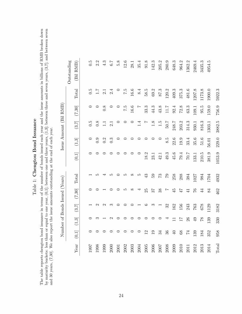
(WIND), which provides information on Chinese financial markets. Table 1 and Figure 1

report the number of bonds issued and the issue amounts from 1997 to 2014. Both the

numbers of bonds issued and the issue amounts are negligible before 2005 but since the

fiscal stimulus in late 2008, chengtou bond market expands dramatically. During the

global financial crisis, Chinese authorities provide a RMB 4 trillion ($250 billion) stimulus

package to counter slowing economic growth. Only RMB 1.2 trillion comes from the central

government; the remainder of RMB 2.8 trillion is provided by local governments (see Lu and

Sun, 2013). Given the restrictions on loans and on municipal bond issuance, municipalities

rely extensively on chengtou bonds to raise funds during this period. The number of bonds

issued in 2009 jumps to 258 compared with just 79 in 2008. The post-2008 average growth

rate of new issues is 85% per year. In 2014, the number of new chengtou bond issues reaches

1,704, with a total amount outstanding of RMB 4.95 trillion ($0.85 trillion).

5

Decomposing the issue amounts of bonds by maturity in Figure 2, the bonds issued before

2008 are mainly long-term and very short-term bonds. Since the global financial crisis of

2007-2008, the bonds issued mainly have a maturity of three to seven years, and these tenors

account for 66% of the total issued bonds in 2014.

Figure 3 shows the relations of important institutions involved in the local government

debt market in China. According to China Central Depository & Clearing Co., outstanding

chengtou bonds are held mainly by commercial banks (31.0%), funds (24.8%), and insurance

companies (21.4%)— the latter two types of investors belong to China’s shadow banking

sector. As the issuers of chengtou bonds, LGFVs do not count its liabilities as official

debt. Nevertheless, LGFV liabilities are backed by local governments, and thus chengtou

bonds represent a very large off-balance sheet obligation. The central government is

ultimately responsible for all local government finances. LGFVs (which include state-owned

enterprises) also have tight business connections with commercial banks.2 LGFVs use the

land transferred from local governments as collateral for bank loans. Thus, many financial

institutions and financing sources are interlinked through issuing, holding, or collateralizing

chengtou bonds.

Given these relations, rapidly decreasing land prices may be a trigger for a systemic event

as LGFV collateral consists of property, land-use, development rights, and other real estate-

related assets. In normal times, land value increases and LGFVs are able to rollover debts

without increasing their costs of financing. In stressed times of low land prices, debt holders

may demand more collateral, which increases financing costs and generates a significant

rollover risk for LGFVs. One way to meet the shortfall is to sell land, but the fire-sale in an

illiquid market would create a vicious circle. Indeed, revenue from the sales of land-use rights

constitutes a principal source of local government revenue. In the United States, decreasing

real estate prices played a major role in many bankruptcies of over-leveraged savings and

loan banks in the 1980s and 1990s (see Case, 2000) and the subprime mortgage crisis of 2007

(see Brunnermeier, 2009). In our empirical work, we investigate how real estate values and

financial market conditions influence chengtou bond prices.

There are other sources of local government revenue besides those associated with

chengtou bonds, including direct transfer from the central government, loans, and municipal

bond issues. Except for chengtou bonds, none of these have market prices.3 In so far as

2Commercial banks cannot directly lend to local governments. According to China’s National AuditOffice, commercial banks are the primary financing source for local governments mainly through their loansto LGFVs.

3Directly issued municipal bonds are sold over-the-counter, and there are no public figures on originalissuance or secondary-market transactions, except for nationwide total issuance information that is published

6

chengtou bonds reflect risk that is shared by other types of local government financing—

credit risk, geography, exposure to local economic growth and real estate conditions, fiscal

health of the issuer and issuing province, among others—the relatively transparent chengtou

bond market provides a window to appraise the risk exposure of Chinese municipalities

in general, and to examine how that risk is related to broad financial market and macro

factors. In particular, the relations we uncover between chengtou bond yields and real

estate variables, and aggregate monetary policy and economic growth factors, are of interest

to the broad policy debate on Chinese local government finances.

2.2 Other Characteristics of Chengtou Bonds

The rapid expansion of chengtou bond market goes hand-in-hand with higher yields, which

is consistent with investors perceiving greater risks with increasing LGFV liabilities. Table 2

reports that yields of newly issued bonds increase from an average value of 3.5% in 2007

to 6.9% in 2014. There are increases in yields even for short-term bonds with a maturity

less than one year; such bonds exhibit yield increases from 2.7% in 2009 to 5.4% in 2014.

Moreover, the average maturity drops from 6.0 years in 2009 to 5.3 years in 2014, implying

that investors prefer shorter-term maturities as the risks of chengtou bonds increase.

Table 3 summarizes chengtou bond issuance by each province. In 2014, there are 30

provinces which issue chengtou bonds. The top five provinces with the largest amounts

outstanding are Jiangsu, Zhejiang, Beijing, Shanghai, and Guangdong. These provinces

represent 40% of the total RMB 2.34 trillion chengtou bonds outstanding. These are all

coastal provinces, except for Beijing which is the capital. The five provinces with the smallest

issuance are Ningxia, Hainan, Jilin, Qinghai, and Shanxi. With the exception of Hainan,

these are all interior provinces.

Chengtou bonds are rated from A to AAA, with the short-term note rating from A1 to

A1+. Each bond is rated at issue by one of the five major credit rating agencies: (i) China

Chengxin International Credit Rating Co., Ltd.(a joint venture with Moody’s); (ii) China

Lianhe Credit Rating Co. Ltd. (a joint venture with Fitch Ratings); (iii) Dagong Global

Credit Rating Co., Ltd.; and (iv) Pengyuan Credit Rating Co., Ltd.; (v) Shanghai Brilliance

Credit Rating & Investors Service Co., Ltd. (in partnership with S&P). We quantify bond

ratings by assigning numerical values, where higher numbers indicate higher credit quality.

We assign a value of six to the highest rated bonds (AAA), a value of one for the lowest

rated bonds (A), and fill in the numbers in between. Except for non-rated bonds (16% of

by the central government.

7

the total issuance), 18% of bonds have a rating of AAA at issue, 27% are rated AA+, and

37% are rated AA. The lower-quality bonds with AA-, A+ and A ratings only account for

1.5% of the total issuance.

2.3 Corruption

2.4 Real Estate

3 Data

In Section 3.1, we define chengtou bond excess yields which constitute the dependent variable

of our analysis. We report considerable heterogeneity in excess yields across time and

provinces in Section 3.2. Sections 3.3 and 3.4 detail our nationwide and province-level macro

variables, respectively. We construct a corruption index in Section 3.5. Finally, Section 3.6

describes various liquidity characteristics of chengtou bond market.

3.1 Chengtou Bond Excess Yields

A well-known fact in fixed income is that all yields are highly correlated with the level of

government bond yields, or the “level” factor (see Knez, Litterman, and Scheinkman, 1994).

We construct yields in excess of matching central government bond yields to isolate the yield

spreads in chengtou bond market. We need to control at least for duration because of the

very different maturities at issue (see Figure 2), but our matching procedure also takes into

account convexity and other effects because we control for all cash flows of the chengtou

bond.

We define the excess yield as the difference between the chengtou bond yield and the

matched central government bond yield:

Yij(t) = yCTBij (t)− yCGB

i (t), (1)

where yCTBij (t) is the yield for chengtou bond i in province j at time t, which we calculate

based on the transaction price at time t. We take the central government bond yield at

time t, yCGBi (t), which has the same cash flow characteristics as chengtou bond i.

To compute the matching central government bond yield, yCGBi (t), we use the zero-

coupon rates of Chinese government bonds, which we compute as follows. We take daily

transaction records from WIND on Chinese central government bonds at time t satisfying

8

the following criteria: (1) there are at least 20 bond transactions, (2) the time-to-maturity

of these bonds spans at least 10 years, and (3) we exclude bonds with remaining maturity

less than one month. We fit the zero curve following Svensson (1994), who assumes the

following functional form for the instantaneous forward rate, f :4

f(m, θ) = β0 + β1 exp

(−mτ1

)+ β2

m

τ1

exp

(−mτ1

)+ β3

m

τ2

exp

(−mτ2

), (2)

where m denotes the time to maturity and θ = (β0, β1, β2, β3, τ1, τ2) are model parameters to

be estimated. The forward curve in equation (2) is understood to apply at time t. Using the

parameterized forward curve, we derive the corresponding zero-coupon central government

bond yield curve at time t over different maturities s, {rs(t)}.To find the matching central government bond yield for chengtou bond i, we hold fixed

bond i’s characteristics—coupon type, coupon rate, coupon frequency, and maturity date—

at the time of trade and discount each cash flow using the central government bond zeros:

PCGBi =

T∑s=1

CCTBi

(1 + rs(t))s+

100

(1 + rT (t))T, (3)

for maturity T , coupon CCTBi and the prevailing central government zero curve at time t

is {rs(t)}. With the implied government bond price PCGBi , we calculate the corresponding

yield, yCGBi , which we define as the matched central government bond yield for chengtou

bond i. Equation (3) effectively prices bond i as a Chinese central government bond because

it uses that series of discount rates (see Duffie and Singleton, 1999), and is thus more accurate

than just matching on duration or maturity because it controls for all the cash flow effects

unique to each chengtou bond.

We calculate the chengtou bond-level excess yields at the daily frequency, and then

aggregate to the monthly frequency and/or province level depending on the research design,

which we detail below. In our final sample, there are 20,357 bond-month observations issued

in 28 provinces from August 2007 to December 2014.

3.2 Excess Yields across Time and Provinces

Under China’s current fiscal and tax system, the central government is ultimately responsible

for all revenues and deficits of local governments. If investors perceive that chengtou bonds

4The Svensson (1994) model produces smaller fitting errors than the Nelson and Siegel (1987) procedure.

9

have an inviolable central government guarantee, there should be no predictable cross-

sectional variation in excess chengtou bond yields and we should expect to observe the

same average chengtou bond yields across provinces. Is this true?

Figure 4 plots the dispersion of excess chengtou bond yields at issue in Panel A and

in the secondary market in Panel B. The graphs reveal that chengtou bond excess yields

are persistent, with a first-order autocorrelation of 0.79. We mark the median value along

with the 10th and 90th deciles from 2005 to 2014. Evidently, there is large heterogeneity

in excess yields across issues, and it occurs in both the primary and secondary markets. In

the primary market, the average range between the 10th and 90th deciles is 2.95% with a

standard deviation of 0.95%. The corresponding range for for the 10th and 90th percentiles

in the secondary market is 1.84% with a standard deviation of 0.87%. Figure 4 shows that

the excess bond dispersion changes over time, and tends to increase when the median excess

yield is high. This suggests that the market more finely distinguishes different underlying

risks of chengtou bonds across provinces when overall market conditions deteriorate.

Table 4 reports the summary statistics of excess yield for the whole sample. Overall,

chengtou bonds earn a premium of 1.98%, on average, over matching central government

bond yields. Table 4 also reports summary statistics of subsamples broken down by province

characteristics based on: 1) geography, 2) real estate rank (measured by the average price

per squared meters during 2008 to 2012), 3) local GDP growth rate, and 4) the local fiscal

gap to GDP ratio. Table 4 shows that there is predictable variation in excess yields across

provinces: more expensive bonds (lower yields) tend to be those issued in provinces located

along the coast, those bonds issued in provinces exhibiting higher housing prices, and issuing

provinces with lower GDP growth rates and smaller fiscal gaps.

In summary, we find large cross-sectional heterogeneity in excess chengtou bond yields

even though chengtou bonds are guaranteed by the Chinese central government; the market

seems to perceive that all chengtou bonds are not equal. We now describe potential risk

factors which may be priced in the cross section of chengtou bonds.

3.3 Nationwide Economic Barometers

We collect national variables to calculate province risk exposures. We select these national

variables on the basis that they capture China’s solvency risk, monetary policy, and financial

market conditions. We employ the following abbreviations:

10

CDS Chinese credit default swap rate

FDI Foreign direct investment in China

CA Log of the current account

FX Effective real exchange rate

RF One-year time deposit interest rate

RET Shanghai stock exchange market return (including all A-shares and B-shares)

Credit default swap rates (CDS), foreign direct investment (FDI), and current account

(CA) all capture different aspects of solvency risk. For monetary policy proxies, we use the

effective real exchange rate (FX) and the one-year time deposit interest rate (RF ). The

latter as the benchmark interest rate in China. For China’s financial market conditions,

we take the Chinese stock market index (including all A-shares and B-shares) and use the

market-weighted return (RET ). The nationwide variables come from WIND, the National

Bureau of Statistics, and Global Financial Data, and are available at the monthly frequency

from January 2005 to December 2014.

3.4 Province-Level Economic Barometers

We expect that chengtou bond yields should reflect the underlying quality and price

dynamics of their collateral, real estate, and general economic growth. We obtain province-

level economic indicators from the National Bureau of Statistics and WIND. These variables

reflect the local economic and fiscal conditions and are all available each year over 2005 to

2014 for each province:

11

GDP Growth Log difference of real GDP

Fiscal Gap Difference of revenue and expenditure, scaled by local GDP

Real Estate GDP Ratio of real estate value-added GDP to total GDP

Service GDP Ratio of service value-added GDP to total GDP

Retail GDP Ratio of wholesale and retail value-added GDP to total GDP

Hotel GDP Ratio of hotel industry value-added GDP to total GDP

Land Cost Total amount of RMB used to purchase land as a ratio of local

GDP

Loans to Real Estate RMB amount of loans to real estate companies in each province

scaled by local GDP

3.5 Corruption Indices

Corruption in China seems to be endemic. The Carnegie Endowment estimates that the

cost of corruption in China in 2003 is $86 billion, or 3% of GDP, and in 2013 this increases

to 13% of GDP.5 Our primary measure of a province’s political risk is the weighted ranking

number of officials named in the graft probes by China’s Central Commission for Discipline

Inspection (CCDI).

We manually compile a list of individual officials in graft investigations published on the

CCDI’s website since 2012 (when President Xi took office) to 2014. There are a total of 753

officials named in the graft probes, covering all 31 provinces. We further collect information

on corrupt officials’ titles and rankings, and categorize individuals into seven rankings. The

final index number, which we denote as Corruption, is a weighted ranking of corrupt officials

in each province. A higher index number suggests more severe corruption for the province,

and hence may correspond to greater political risk. We also use the number of officials listed

in the graft cases in each province as an alternative proxy of political risk, which we denote

as Number of Corruption Cases. The average corruption index number is 2.1 with a standard

deviation of 0.4 across 30 provinces whose LGFVs issue chengtou bonds. On average, there

are 21.2 cases investigated for each province, with a standard deviation of 13.7 cases. The

number of officials named in the graft report varies across provinces: Tianjin and Guangxi,

5See www.carnegieendowment.org/files/pb55_pei_china_corruption_final.pdf. In 2012, theCommunist Party of China launches an anti-corruption campaign. Following President Xi’s proclamation,the CCDI is “striking tigers and flies at the same time”—a reference to investigating corrupt high- andlow-level officials.

12

for example, each have four cases in our sample, whereas Shanxi has 49 cases, and Sichuan

and Hubei have 50 and 51 cases, respectively.

3.6 Liquidity

After issuance, chengtou bonds trade mainly in the interbank market, which has a market

share of 68%. They also trade in the Shanghai and Shenzhen stock exchanges, with these

venues capturing a market share of 30%. For each bond transaction on day t, we observe its

open and closing prices, the highest and lowest price, the mid price, trading volume, and the

yield to maturity. To obtain accurate bond pricing information, we only keep bonds which

trade on the interbank or exchange markets, and screen out bonds with special terms such

as callable or putable bonds.

To get a sense of the overall market liquidity, we calculate the trading frequency as the

number of traded bonds divided by the total number of outstanding bonds in each month.

The monthly trading frequency is below 30% before 2006, jumps to 65% in 2007, remains

stable between 60% to 70% after August 2007. Given our object of interest is the cross

section of chengtou bonds, we choose our final sample to cover the relatively liquid period

from August 2007 to December 2014.

We compute three bond-level liquidity statistics:

Turnover is the ratio of trading volume to the outstanding amount, which we compute at the

monthly frequency. We sum across trading days within each month to obtain the monthly

trading volume. We take the amount outstanding at the end of the month.

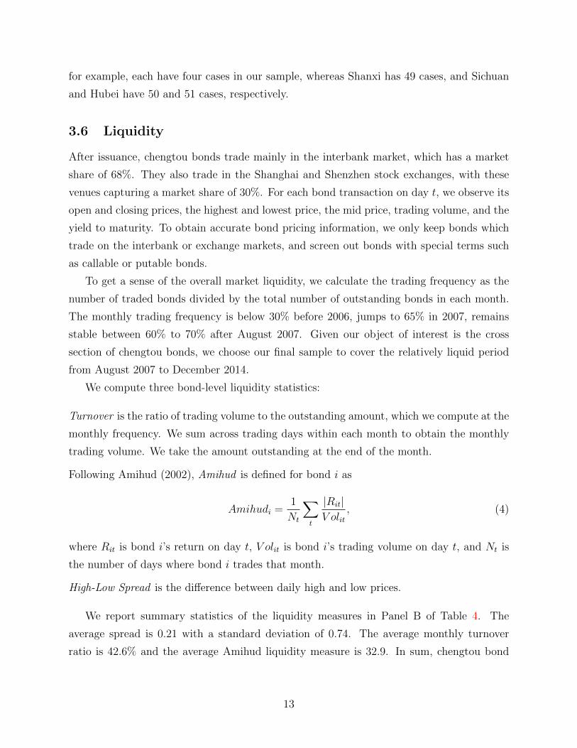
Following Amihud (2002), Amihud is defined for bond i as

Amihudi =1

Nt

∑t

|Rit|V olit

, (4)

where Rit is bond i’s return on day t, V olit is bond i’s trading volume on day t, and Nt is

the number of days where bond i trades that month.

High-Low Spread is the difference between daily high and low prices.

We report summary statistics of the liquidity measures in Panel B of Table 4. The

average spread is 0.21 with a standard deviation of 0.74. The average monthly turnover

ratio is 42.6% and the average Amihud liquidity measure is 32.9. In sum, chengtou bond

13

market is relatively illiquid.6 Thus, we might expect the cross section of chengtou bonds to

exhibit an illiquidity premium, as is the case for equity and bond markets (see, for example,

Pastor and Stambaugh, 2003, and Bao, Pan, and Wang, 2011, respectively).

4 Empirical Results

We first investigate how nationwide risk variables are priced in the cross section of chengtou

bond yields. Section 4.1 details how we compute province risk exposures, and we estimate the

coefficients on those risk exposures in cross-sectional regressions in Section 4.2. Sections 4.3

to 4.5 discuss how real estate risk, political risk, and liquidity characteristics are priced,

respectively.

4.1 Risk Exposures

We compute province-level betas with respect to national macroeconomic and financial

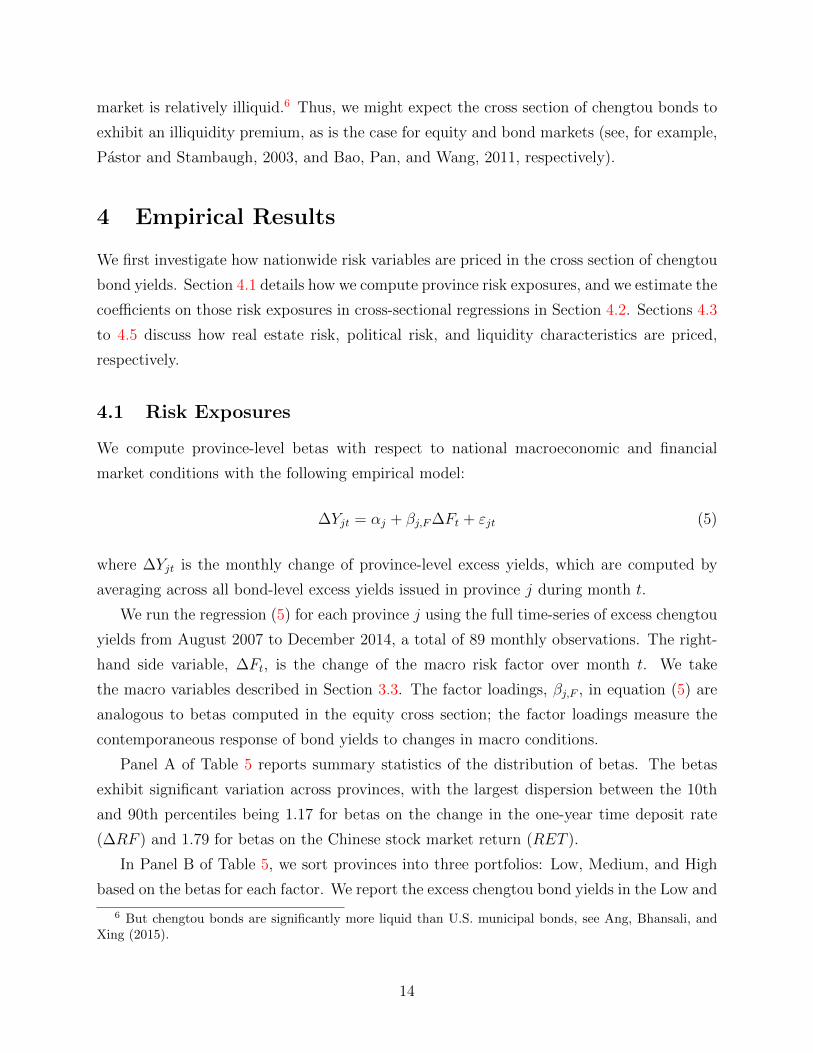
market conditions with the following empirical model:

∆Yjt = αj + βj,F∆Ft + εjt (5)

where ∆Yjt is the monthly change of province-level excess yields, which are computed by

averaging across all bond-level excess yields issued in province j during month t.

We run the regression (5) for each province j using the full time-series of excess chengtou

yields from August 2007 to December 2014, a total of 89 monthly observations. The right-

hand side variable, ∆Ft, is the change of the macro risk factor over month t. We take

the macro variables described in Section 3.3. The factor loadings, βj,F , in equation (5) are

analogous to betas computed in the equity cross section; the factor loadings measure the

contemporaneous response of bond yields to changes in macro conditions.

Panel A of Table 5 reports summary statistics of the distribution of betas. The betas

exhibit significant variation across provinces, with the largest dispersion between the 10th

and 90th percentiles being 1.17 for betas on the change in the one-year time deposit rate

(∆RF ) and 1.79 for betas on the Chinese stock market return (RET ).

In Panel B of Table 5, we sort provinces into three portfolios: Low, Medium, and High

based on the betas for each factor. We report the excess chengtou bond yields in the Low and

6 But chengtou bonds are significantly more liquid than U.S. municipal bonds, see Ang, Bhansali, andXing (2015).

14

High portfolios, along with a t-test for the average difference. There are significant differences

in the excess yields for all the macro factors, except for the exchange rate betas. Provinces

with higher betas to China’s CDS tend to have higher yields, with the difference between

the Low and High portfolios being -0.24%. Provinces with higher betas to direct foreign

investment also tend to have higher yields. These univariate portfolio sorts suggest that

chengtou bonds reflect macroeconomic, credit, monetary policy, and financial conditions.

We now formally estimate prices of risks for these nationwide risk factors in a cross-sectional

regression, which is able to jointly control for the effect of multiple risk factors.

4.2 The Price of Macro Risk

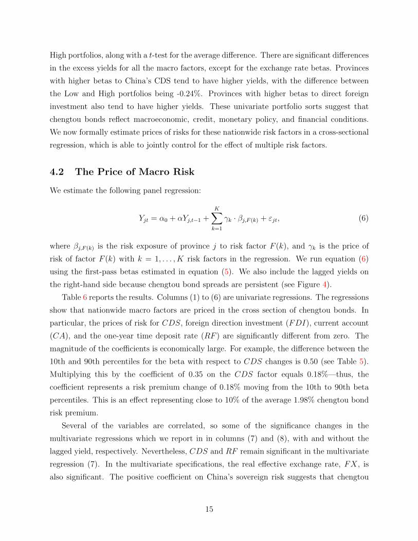
We estimate the following panel regression:

Yjt = α0 + αYj,t−1 +K∑k=1

γk · βj,F (k) + εjt, (6)

where βj,F (k) is the risk exposure of province j to risk factor F (k), and γk is the price of

risk of factor F (k) with k = 1, . . . , K risk factors in the regression. We run equation (6)

using the first-pass betas estimated in equation (5). We also include the lagged yields on

the right-hand side because chengtou bond spreads are persistent (see Figure 4).

Table 6 reports the results. Columns (1) to (6) are univariate regressions. The regressions

show that nationwide macro factors are priced in the cross section of chengtou bonds. In

particular, the prices of risk for CDS, foreign direction investment (FDI), current account

(CA), and the one-year time deposit rate (RF ) are significantly different from zero. The

magnitude of the coefficients is economically large. For example, the difference between the

10th and 90th percentiles for the beta with respect to CDS changes is 0.50 (see Table 5).

Multiplying this by the coefficient of 0.35 on the CDS factor equals 0.18%—thus, the

coefficient represents a risk premium change of 0.18% moving from the 10th to 90th beta

percentiles. This is an effect representing close to 10% of the average 1.98% chengtou bond

risk premium.

Several of the variables are correlated, so some of the significance changes in the

multivariate regressions which we report in in columns (7) and (8), with and without the

lagged yield, respectively. Nevertheless, CDS and RF remain significant in the multivariate

regression (7). In the multivariate specifications, the real effective exchange rate, FX, is

also significant. The positive coefficient on China’s sovereign risk suggests that chengtou

15

bonds are economically levered versions of sovereign credit risk—the larger the exposure

to China’s solvency risk, the higher are chengtou bond yields. The negative coefficient on

the real effective exchange rate may be due to government finances in provinces with high

exchange rate betas benefiting from increased exports when the RMB depreciates.

Finally, the regression (8) contains the lagged yield. This carries a large, positive

coefficient of 0.72 because spreads are persistent. In the presence of the lagged yield, the

CDS spread and the real effective exchange rate remain significant with the same signs as

in regression (7).

We now turn to examining province-level and bond-level variables. In the terminology

of asset pricing, we now include characteristics in the cross-sectional regression as opposed

to just factor loadings (cf. Daniel and Titman, 1997). We still include the betas with

respect to CDS, FX, and RF . Even though the province exposure to China’s benchmark

interest rate risk is marginally significant after controlling for other explanatory variables, it

is significant in regression (7). Taking a conservative stance, we include these betas in our

extended regressions investigating the role of real estate, political risk, and liquidity in the

following sections.

4.3 Real Estate

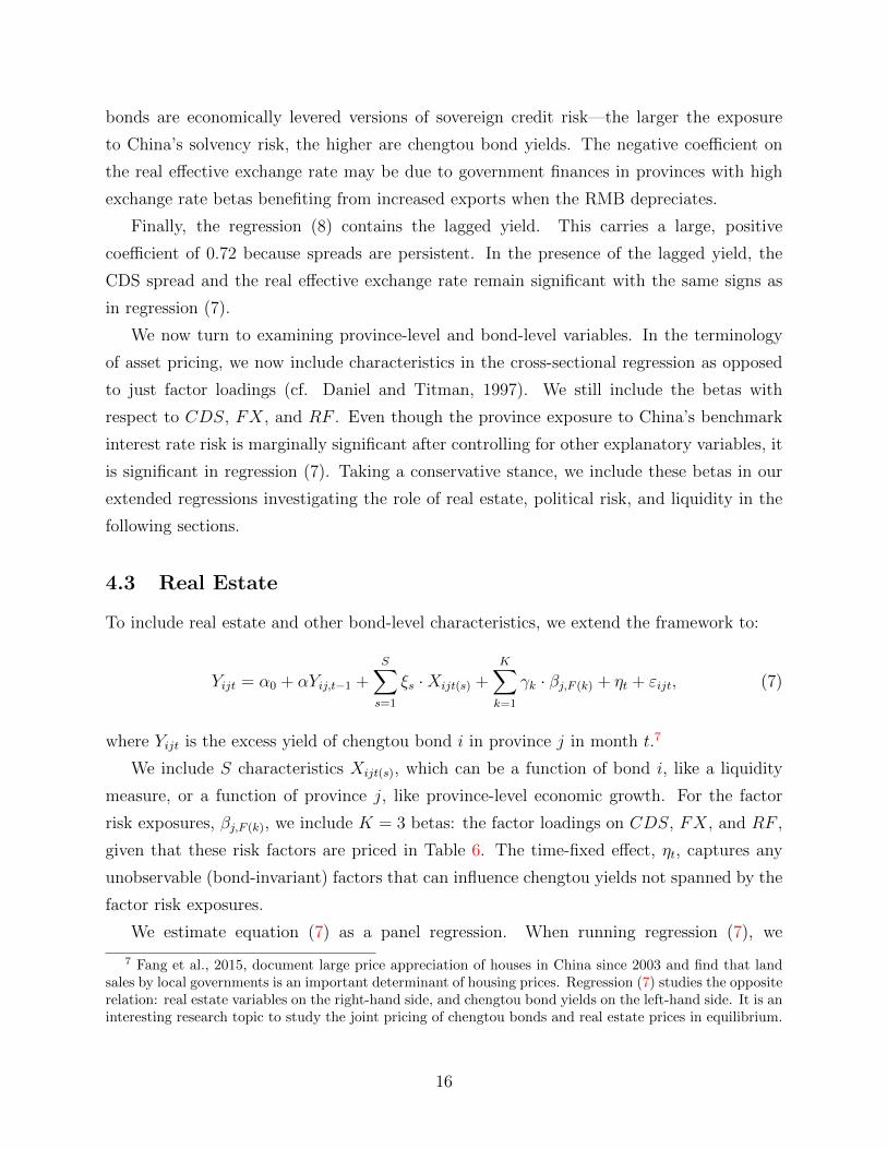
To include real estate and other bond-level characteristics, we extend the framework to:

Yijt = α0 + αYij,t−1 +S∑

s=1

ξs ·Xijt(s) +K∑k=1

γk · βj,F (k) + ηt + εijt, (7)

where Yijt is the excess yield of chengtou bond i in province j in month t.7

We include S characteristics Xijt(s), which can be a function of bond i, like a liquidity

measure, or a function of province j, like province-level economic growth. For the factor

risk exposures, βj,F (k), we include K = 3 betas: the factor loadings on CDS, FX, and RF ,

given that these risk factors are priced in Table 6. The time-fixed effect, ηt, captures any

unobservable (bond-invariant) factors that can influence chengtou yields not spanned by the

factor risk exposures.

We estimate equation (7) as a panel regression. When running regression (7), we

7 Fang et al., 2015, document large price appreciation of houses in China since 2003 and find that landsales by local governments is an important determinant of housing prices. Regression (7) studies the oppositerelation: real estate variables on the right-hand side, and chengtou bond yields on the left-hand side. It is aninteresting research topic to study the joint pricing of chengtou bonds and real estate prices in equilibrium.

16

standardize the explanatory characteristic variables in the cross section each month. We

do not standardize the lag of the excess yield or the betas. In this way, the estimated

coefficients in the regression can be interpreted as the effect of a one standard deviation

move in the cross section, so the economic scale is also comparable across variables. We take

values of the characteristics available at time t, which are the figures made available at the

end of the previous year prior to time t.

In Table 7, we investigate how real estate variables influence the cross section of chengtou

bonds. In Panel A, we report the univariate regression coefficients taking just one real estate

variable at a time. The effects of real estate risk are large. The coefficient on real estate

GDP is -0.17, implying that if a given province moved by one standard deviation in the

cross section, that province’s chengtou bond yields would decrease by 0.17%. Given that

the average excess chengtou bond yield is 1.98%, this is a large economic effect. Note that

all the real estate regressions have relatively high R2s of approximately 20%.

In Panel A, all the real estate variables are significant, but there are differences in sign.

A priori we might expect that, like the negative coefficient on real estate GDP, higher real

estate-related economic growth should indicate a lower risk of default because of higher

collateral values, and thus lower yields. The coefficients for hotel GDP, GDP growth in

general, and the fiscal gap, however, are positive. At first glance, this relation seems counter-

intuitive. The reason for this unexpected sign is that provinces with higher GDP growth

and higher fiscal surpluses also exhibit higher volatilities of growth.

Suppose we divide the provinces into High, Middle, and Low terciles similar to Table 4.

Then provinces in the High tercile of fiscal surpluses have a mean of 20.7% and a standard

deviation of 9.9%. The provinces in the Low fiscal surplus tercile have, by construction, the

lowest mean of fiscal surpluses of 3.2% but also a low standard deviation of 3.0%. The same

findings apply to GDP growth: the provinces with the highest average GDP growth also

have the most volatile growth. The mechanical relation between high economic growth and

high volatility drives the positive coefficients in the univariate regressions in Table 7, Panel

A as these provinces are actually risky!

Panel B of Table 7 reports multivariate regression results. Regression (1) jointly takes

the various GDP components. Real estate GDP and service GDP stand out, both with

negative coefficients. In regression (2), we confirm the findings of the univariate regression

that both variables positively predict excess chengtou bond yields, but this is driven by the

positive relation between these economic variables and macro variability. In regression (3),

we consider the full set of province-level macro variables. This regression favors real estate

17

GDP and service GDP. Regression (4) adds the betas with respect to CDS, FX, and RF .

Regression (5) further adds bond rating as a control variable. In all the specifications, real

estate GDP remains statistically significant. In regression (4) and (5), other province macro

variables have insignificant effects on bond yields, after controlling for province-level risks.

4.4 Political Risk

In Table 8, we run cross-sectional regressions (equation (7)) with our two political risk

variables measuring corruption: the corruption index and the number of corruption cases,

which we define in Section 3.5. We consider the corruption series individually in regressions

(1) and (2). Both variables are significant, with higher levels of corruption corresponding to

higher yields. A one standard deviation move of a province in the cross section from less to

more corrupt increases excess chengtou bond yields by 0.09% for the corruption index and

0.05% for the number of corruption cases, respectively. The adjusted R2s for these univariate

regression is around 20%, which is relatively high because we use time fixed effects.

In regressions (3) to (5), we add the control variables: the betas with respect to CDS,

FX, and RF changes, bond rating, and the lagged yield. In the presence of these risk

characteristics, there is still a positive and highly statistically significant relation between

the level of corruption and chengtou bond yields.

The negative coefficient on the bond rating in Table 8 is also interesting. Because of

the way we construct the rating variable, higher values correspond to higher ratings. Thus,

the significant negative coefficient on the rating variable indicates that bonds with higher

ratings have lower yields. The fact that there are other significant variables in the regressions

suggest that the ratings do not capture all the cross-sectional variation in chengtou bond

yields.

To understand better how the corruption index is related to real estate variables, we run

cross-sectional regression of province-level corruption on the local real estate value-added

GDP ratio, which is the most significant variable in the previous test of Section 4.3. We

discover a significant negative relationship between province corruption, using either proxy

of corruption index or number of corruption cases, and the real estate GDP in Table 9. One

standard deviation increase of a province in the cross section from lower to higher real estate

GDP ratio reduces the corruption index by 0.32%, or reduces the number of corruption cases

by 17%. The results remain robust after controlling province risk exposures to aggregate

credit risk and monetary policy. The strong performance suggests that the influence of

corruption on local government credit spreads is likely through the real estate channel.

18

4.5 Liquidity

Our final specifications investigate if liquidity is priced. In the first three regressions of

Table 10, we examine turnover, the Amihud (2002) measure, and the High-Low spread,

which is the difference between daily high and low prices. In the univariate regressions, only

turnover and the Amihud measure are statistically significant. For the Amihud measure, a

one standard deviation increase leads to a decrease of 0.04% in chengtou bond yields. The

Amihud measure becomes insignificant in regression (4), controlling for all three liquidity

variables jointly, and in regressions (5) to (7) with the CDS, FX, and RF risk factor

exposures, and lagged yields, respectively. Only the turnover ratio remains robust in the

presence of province-level risk exposures, credit ratings, and the lagged yield in regressions(4)

to (6).

The turnover coefficient is statistically significant across all regression specifications.

The coefficient, however, is surprisingly positive: bonds with higher turnover should be

more liquid bonds, and this should lead to lower yields as the greater liquidity should be

attractive to investors. The positive sign between turnover and yields is reminiscent of the

positive relation between volume and returns which Gervais, Kaniel, and Mingelgrin (2001)

find in equity markets. Gervais, Kaniel, and Mingelgrin postulate that their finding of higher

liquidity-higher returns is when a stock becomes more visible, it draws in a large number of

potential buyers while the number of potential sellers remains the same. In the presence of

short-sale constraints, the increase in visibility tends to increase expected returns (cf. Miller,

1977; Harrison and Kreps, 1978). Chinese markets fit these particular circumstances. Short-

selling of securities is not permitted. Mei and Xiong (2009) note that speculative investors

play a pronounced role in Chinese markets.

There is another possible channel contributing to the positive correlation between current

turnover and chentou bond yields in the cross section. Speculators are most drawn to those

bonds with the highest yields—the riskiest bonds. Consistent with this “reaching for yield,”

turnover is highest at 52.4% for AA-rated bonds, and lowest at 32.4% for AAA-rated bonds.

In regression (7), we introduce an interaction term between turnover and high-quality

bonds. The latter variable is a dummy which is equal to one if the bond credit rating

is AAA, and zero otherwise. Although the Amihud measure is insignificant in the

multivariate regressions (regressions (4) to (6)), it is significant in the univariate specification

(regression(2)), so for completeness we also include an interaction term between the Amihud

measure and high-quality bonds. Table 10, regression (7) shows that while the coefficient

on turnover remains significantly positive, the coefficient on the interaction term between

19

turnover and high quality is negative. Thus, within the high credit quality category, bonds

with high turnover ratios have lower yields.

5 Conclusion

Chengtou bonds play an important role in funding Chinese local governments. The market

experiences tremendous growth after the 2008 global financial crisis and as of December 2014,

there are RMB 4.95 trillion ($0.82 trillion) of chengtou bonds outstanding. The Chinese

central government is ultimately responsible for the finances of all local governments, but

despite the guarantee, we find large heterogeneity in chengtou bond yields.

Reflecting the systemic risk of chengtou bonds, we find that variables reflecting aggregate

credit risk, monetary policy, and the real effective exchange rate are priced in the cross

section. We find that real estate values are important drivers of chengtou bonds, which is not

surprising given that their collateral value is directly linked to the real estate market. We also

find that chengtou bond yields reflect corruption risk: we construct an index of corruption

based on officials investigated by the Central Commission for Discipline Inspection (CCDI).

We find a significantly positive correlation between risk-adjusted chengtou bond yields and

the corruption index.

The rules governing local government finances in China are changing. In October

2014, the State Council issues Rule No. 43 which states that starting from January 1,

2016, LGFVs are no longer allowed to issue chengtou bonds. This effectively shuts down

chengtou bonds as a source of funds for local governments. Instead, local governments

will rely on alternative financing channels: (1) issuing regular municipal bonds for public-

interest projects fully backed by tax revenue, (2) forming public-private partnerships for

infrastructure developments which do not carry a government guarantee, and (3) issuing

private corporate debt for non-public (commercial) real estate projects.

These developments mean that although the amounts outstanding are large, chengtou

bonds are likely to become a legacy asset. At present, chengtou bonds are the only local

government asset where market prices are observable. Thus, the pricing of credit risk,

political risk, real estate risk, and other province and bond-level characteristics in chengtou

bonds provides a unique opportunity to study how these types of risk impact Chinese local

government finances in general.

20

References

[1] Allen, F., J. Qian, and M. Qian, 2005. Law, finance and economic growth in China.

Journal of Financial Economics 77, 57-116.

[2] Amihud, Y., 2002. Illiquidity and stock returns: Cross-section and time-series effects.

Journal of Financial Markets 5, 31-56.

[3] Ang, A., V. Bhansali, and Y. Xing, 2015. The muni bond spread: Credit, liquidity, and

tax. Working paper, Columbia Business School.

[4] Bao, J., J. Pan, and J. Wang, 2011. The illiquidity of corporate bonds. Journal of

Finance 66, 911-946.

[5] Brunnermeier, M. K., 2009. Deciphering the liquidity and credit crunch 2007-2008.

Journal of Economic Perspectives 23, 77-100.

[6] Butler, Alexander W., Larry Fauver, and Sandra Mortal, 2009. Corruption, Political

Connections, and Municipal Finance. Review of Financial Studies 22, 2873-2905.

[7] Cai, Hongbin, J. Vernon Henderson, and Qinghua Zhang, 2013. China’s land market

auctions: evidence of corruption? The RAND Journal of Economics Volume 44, Issue

3, 488521.

[8] Case, K. E., 2000, Real estate and the macroeconomy, in Glaeser, E. L., and J. A.

Parker, Brookings Papers on Economic Activity vol. 2000, no. 2, 119-162, Brookings

Institution Press.

[9] Daniel, K., and S. Titman, 1997. Evidence on the characteristics of cross sectional

variation in stock returns. Journal of Finance 52, 1-33.

[10] Duffie, D., and K. J. Singleton, 1999. Modeling term structures of defaultable bonds.

Review of Financial Studies 12, 687-720

[11] Fang, H., Q. Gu, W. Xiong, and L.A. Zhou, 2015. Demystifying the Chinese housing

boom. Working paper, Princeton University.

[12] Fisman, R., and Y. Wang, 2011. Evidence on the existence and impact of corruption in

state asset sales in China. Working paper, Columbia University.

21

[13] Fisman, R., and Y. Wang, 2013. The mortality cost of political connections. Working

paper, Columbia University.

[14] Gervais, S., R. Kaniel, and D. H. Mingelgrin, 2001. The high volume-return premium.

Journal of Finance 56, 877-919.

[15] Gospodinov, Nikolay, Brian Robertson, and Paula Tkac, 2014. Do Municipal Bonds

Pose a Systemic Risk? Evidence from the Detroit Bankruptcy. Working paper at Federal

Reserve Bank of Atlanta.

[16] Harrison, M., and D. Kreps, 1978. Speculative investor behavior in a stock market with

heterogeneous expectations. Quarterly Journal of Economics 92, 323-336.

[17] Husain, A. M., A. Mody, and K. S. Rogoff, 2005. Exchange rate regime durability and

performance in developing versus advanced economies. Journal of Monetary Economics

52, 35-64.

[18] Knez, P. J., R. Litterman, and J. Scheinkman, 1994. Explorations into factors explaining

money market returns. Journal of Finance 49, 1861-1882.

[19] Levy, A., and S. Schich, 2010. The design of government guarantees for bank bonds:

Lessons from the recent financial crisis. OECD Journal: Financial Market Trends

2010/1.

[20] Li, H., and L. A. Zhou, 2005. Political turnover and economic performance: the incentive

role of personnel control in China. Journal of Public Economics 89, 1743-1762.

[21] Ang, Andrew and Francis Longstaff, 2014. Systemic Sovereign Credit Risk: Lessons

from the U.S. and Europe. Journal of Monetary Economics, forthcoming.

[22] Lu, Y., and T. Sun, 2013. Local government financing platforms in China: A fortune

or misfortune? IMF working paper 13/243.

[23] Mei, J., and W. Xiong, 2009. Speculative trading and stock prices: Evidence from

Chinese A-B share premia. Annals of Economics and Finance 10, 225-255.

[24] Miller, E. M., 1977. Risk, uncertainty, and divergence of opinion. Journal of Finance

32, 1151-68.

[25] Nelson, C. R. and A. F. Siegel, 1987. Parsimonious modeling of yield curves. Journal

of Business 60, 473-89.

22

[26] Pastor, L., and R. F. Stambaugh, 2003. Liquidity risk and expected stock returns.

Journal of Political Economy 111, 642-685.

[27] Svensson, L. E., 1994. Estimating and interpreting forward interest rates: Sweden 1992-

1994. NBER Working Paper 4871.

[28] Wang, S., and F. Yu, 2014. What drives Chinese local government bond yields? Working

paper.

[29] Wu, X., and He, H., 2014. China financial policy report: 201. China Finance Publishing

House.

23

Tab

le1:

Chengto

uBond

Issu

ance

Th

eta

ble

rep

orts

chen

gtou

bon

dis

suan

cein

term

sof

the

nu

mb

erof

bon

ds

issu

edea

chye

ar

and

the

issu

eam

ou

nts

inb

illi

on

sof

RM

Bb

roke

nd

own

by

mat

uri

tyb

uck

ets:

less

than

oreq

ual

toon

eye

ar,

(0,1

];b

etw

een

on

ean

dth

ree

yea

rs,

(1,3

];b

etw

een

thre

ean

dse

ven

years

,(3

,7];

an

db

etw

een

seve

nan

d30

year

s,(7

,30]

.W

eal

sore

por

tth

eis

sue

amou

nts

ou

tsta

nd

ing

at

the

end

of

each

yea

r.

Nu

mb

erof

Bon

ds

Issu

ed(Y

ears

)Is

sue

Am

ount

(Bil

RM

B)

Ou

tsta

nd

ing

Yea

r(0

,1]

(1,3

](3

,7]

(7,3

0]T

otal

(0,1

](1

,3]

(3,7

](7

,30]

Tota

l(B

ilR

MB

)

1997

00

10

10

00.

50

0.5

0.5

1998

03

20

50

0.9

0.8

01.

72.2

1999

01

21

40

0.2

1.1

0.8

2.1

4.3

2000

02

30

50

0.3

2.1

02.

46.7

2001

00

00

00

00

00

5.8

2002

00

05

50

00

7.5

7.5

12.6

2003

00

08

80

00

16.6

16.6

28.1

2004

00

14

50

01.

47

8.4

35.4

2005

12

06

2543

18.2

07

33.3

58.

591.8

2006

19

03

3759

23.1

01.

844

.369.

2142.3

2007

34

01

3873

42.1

01.

543

.887.

3205.2

2008

36

432

779

49.3

8.5

50.7

11.7

120

.2280.9

2009

40

11162

4525

845

.622

.624

8.7

92.4

409

.3648.3

2010

68

17156

4728

879

.419

.920

3.2

72.8

375

.3964.2

2011

74

26243

4138

470

.733

.431

4.3

63.3

481

.61362.2

2012

139

49763

7610

2713

3.1

35.6

930.

110

9.1

120

7.8

2469.4

2013

184

78678

4498

421

0.5

51.6

816.

395

.5117

3.8

3435.3

2014

352

139

1129

8417

0438

1.9

56.0

113

03.1

159.

0190

0.0

4954.5

Tota

l95

833

031

8246

249

3210

53.9

229.

038

82.5

756.

9592

2.3

24

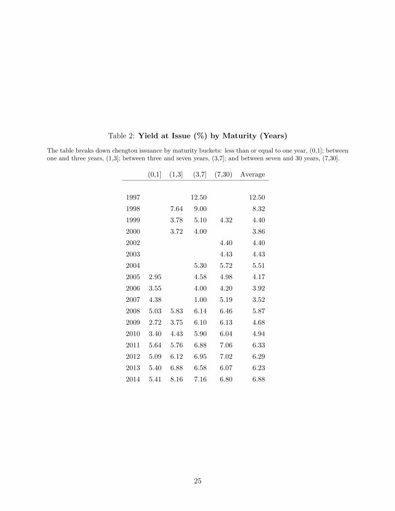
Table 2: Yield at Issue (%) by Maturity (Years)

The table breaks down chengtou issuance by maturity buckets: less than or equal to one year, (0,1]; betweenone and three years, (1,3]; between three and seven years, (3,7]; and between seven and 30 years, (7,30].

(0,1] (1,3] (3,7] (7,30) Average

1997 12.50 12.50

1998 7.64 9.00 8.32

1999 3.78 5.10 4.32 4.40

2000 3.72 4.00 3.86

2002 4.40 4.40

2003 4.43 4.43

2004 5.30 5.72 5.51

2005 2.95 4.58 4.98 4.17

2006 3.55 4.00 4.20 3.92

2007 4.38 1.00 5.19 3.52

2008 5.03 5.83 6.14 6.46 5.87

2009 2.72 3.75 6.10 6.13 4.68

2010 3.40 4.43 5.90 6.04 4.94

2011 5.64 5.76 6.88 7.06 6.33

2012 5.09 6.12 6.95 7.02 6.29

2013 5.40 6.88 6.58 6.07 6.23

2014 5.41 8.16 7.16 6.80 6.88

25

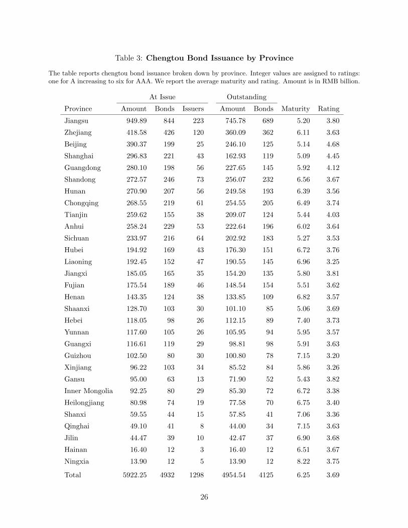
Table 3: Chengtou Bond Issuance by Province

The table reports chengtou bond issuance broken down by province. Integer values are assigned to ratings:one for A increasing to six for AAA. We report the average maturity and rating. Amount is in RMB billion.

At Issue Outstanding

Province Amount Bonds Issuers Amount Bonds Maturity Rating

Jiangsu 949.89 844 223 745.78 689 5.20 3.80

Zhejiang 418.58 426 120 360.09 362 6.11 3.63

Beijing 390.37 199 25 246.10 125 5.14 4.68

Shanghai 296.83 221 43 162.93 119 5.09 4.45

Guangdong 280.10 198 56 227.65 145 5.92 4.12

Shandong 272.57 246 73 256.07 232 6.56 3.67

Hunan 270.90 207 56 249.58 193 6.39 3.56

Chongqing 268.55 219 61 254.55 205 6.49 3.74

Tianjin 259.62 155 38 209.07 124 5.44 4.03

Anhui 258.24 229 53 222.64 196 6.02 3.64

Sichuan 233.97 216 64 202.92 183 5.27 3.53

Hubei 194.92 169 43 176.30 151 6.72 3.76

Liaoning 192.45 152 47 190.55 145 6.96 3.25

Jiangxi 185.05 165 35 154.20 135 5.80 3.81

Fujian 175.54 189 46 148.54 154 5.51 3.62

Henan 143.35 124 38 133.85 109 6.82 3.57

Shaanxi 128.70 103 30 101.10 85 5.06 3.69

Hebei 118.05 98 26 112.15 89 7.40 3.73

Yunnan 117.60 105 26 105.95 94 5.95 3.57

Guangxi 116.61 119 29 98.81 98 5.91 3.63

Guizhou 102.50 80 30 100.80 78 7.15 3.20

Xinjiang 96.22 103 34 85.52 84 5.86 3.26

Gansu 95.00 63 13 71.90 52 5.43 3.82

Inner Mongolia 92.25 80 29 85.30 72 6.72 3.38

Heilongjiang 80.98 74 19 77.58 70 6.75 3.40

Shanxi 59.55 44 15 57.85 41 7.06 3.36

Qinghai 49.10 41 8 44.00 34 7.15 3.63

Jilin 44.47 39 10 42.47 37 6.90 3.68

Hainan 16.40 12 3 16.40 12 6.51 3.67

Ningxia 13.90 12 5 13.90 12 8.22 3.75

Total 5922.25 4932 1298 4954.54 4125 6.25 3.69

26

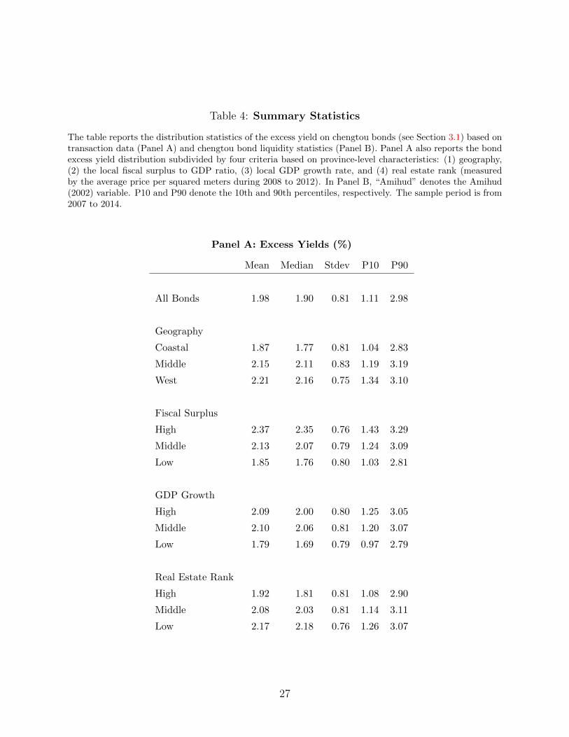
Table 4: Summary Statistics

The table reports the distribution statistics of the excess yield on chengtou bonds (see Section 3.1) based ontransaction data (Panel A) and chengtou bond liquidity statistics (Panel B). Panel A also reports the bondexcess yield distribution subdivided by four criteria based on province-level characteristics: (1) geography,(2) the local fiscal surplus to GDP ratio, (3) local GDP growth rate, and (4) real estate rank (measuredby the average price per squared meters during 2008 to 2012). In Panel B, “Amihud” denotes the Amihud(2002) variable. P10 and P90 denote the 10th and 90th percentiles, respectively. The sample period is from2007 to 2014.

Panel A: Excess Yields (%)

Mean Median Stdev P10 P90

All Bonds 1.98 1.90 0.81 1.11 2.98

Geography

Coastal 1.87 1.77 0.81 1.04 2.83

Middle 2.15 2.11 0.83 1.19 3.19

West 2.21 2.16 0.75 1.34 3.10

Fiscal Surplus

High 2.37 2.35 0.76 1.43 3.29

Middle 2.13 2.07 0.79 1.24 3.09

Low 1.85 1.76 0.80 1.03 2.81

GDP Growth

High 2.09 2.00 0.80 1.25 3.05

Middle 2.10 2.06 0.81 1.20 3.07

Low 1.79 1.69 0.79 0.97 2.79

Real Estate Rank

High 1.92 1.81 0.81 1.08 2.90

Middle 2.08 2.03 0.81 1.14 3.11

Low 2.17 2.18 0.76 1.26 3.07

27

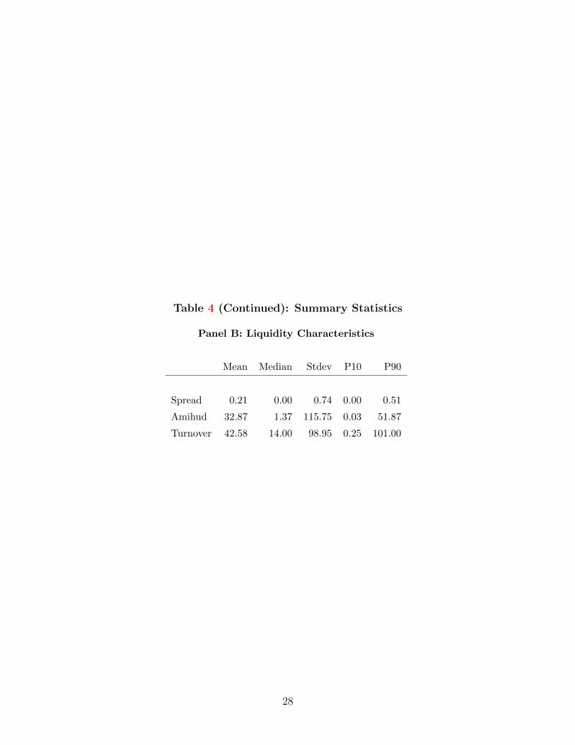
Table 4 (Continued): Summary Statistics

Panel B: Liquidity Characteristics

Mean Median Stdev P10 P90

Spread 0.21 0.00 0.74 0.00 0.51

Amihud 32.87 1.37 115.75 0.03 51.87

Turnover 42.58 14.00 98.95 0.25 101.00

28

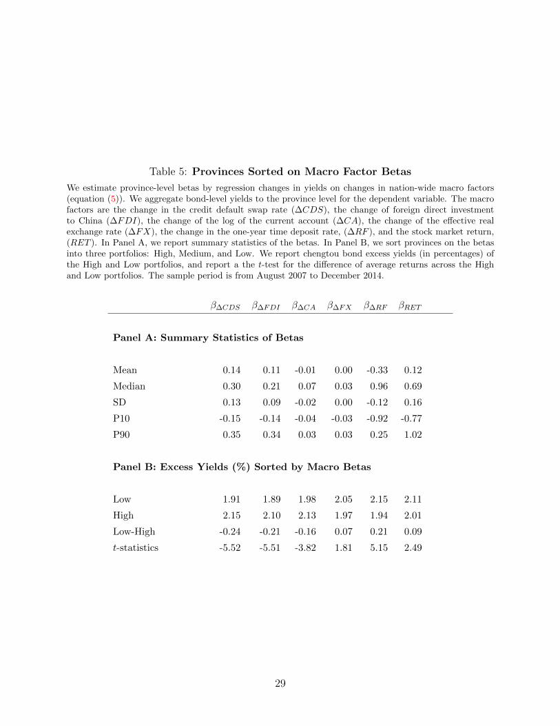
Table 5: Provinces Sorted on Macro Factor Betas

We estimate province-level betas by regression changes in yields on changes in nation-wide macro factors(equation (5)). We aggregate bond-level yields to the province level for the dependent variable. The macrofactors are the change in the credit default swap rate (∆CDS), the change of foreign direct investmentto China (∆FDI), the change of the log of the current account (∆CA), the change of the effective realexchange rate (∆FX), the change in the one-year time deposit rate, (∆RF ), and the stock market return,(RET ). In Panel A, we report summary statistics of the betas. In Panel B, we sort provinces on the betasinto three portfolios: High, Medium, and Low. We report chengtou bond excess yields (in percentages) ofthe High and Low portfolios, and report a the t-test for the difference of average returns across the Highand Low portfolios. The sample period is from August 2007 to December 2014.

β∆CDS β∆FDI β∆CA β∆FX β∆RF βRET

Panel A: Summary Statistics of Betas

Mean 0.14 0.11 -0.01 0.00 -0.33 0.12

Median 0.30 0.21 0.07 0.03 0.96 0.69

SD 0.13 0.09 -0.02 0.00 -0.12 0.16

P10 -0.15 -0.14 -0.04 -0.03 -0.92 -0.77

P90 0.35 0.34 0.03 0.03 0.25 1.02

Panel B: Excess Yields (%) Sorted by Macro Betas

Low 1.91 1.89 1.98 2.05 2.15 2.11

High 2.15 2.10 2.13 1.97 1.94 2.01

Low-High -0.24 -0.21 -0.16 0.07 0.21 0.09

t-statistics -5.52 -5.51 -3.82 1.81 5.15 2.49

29

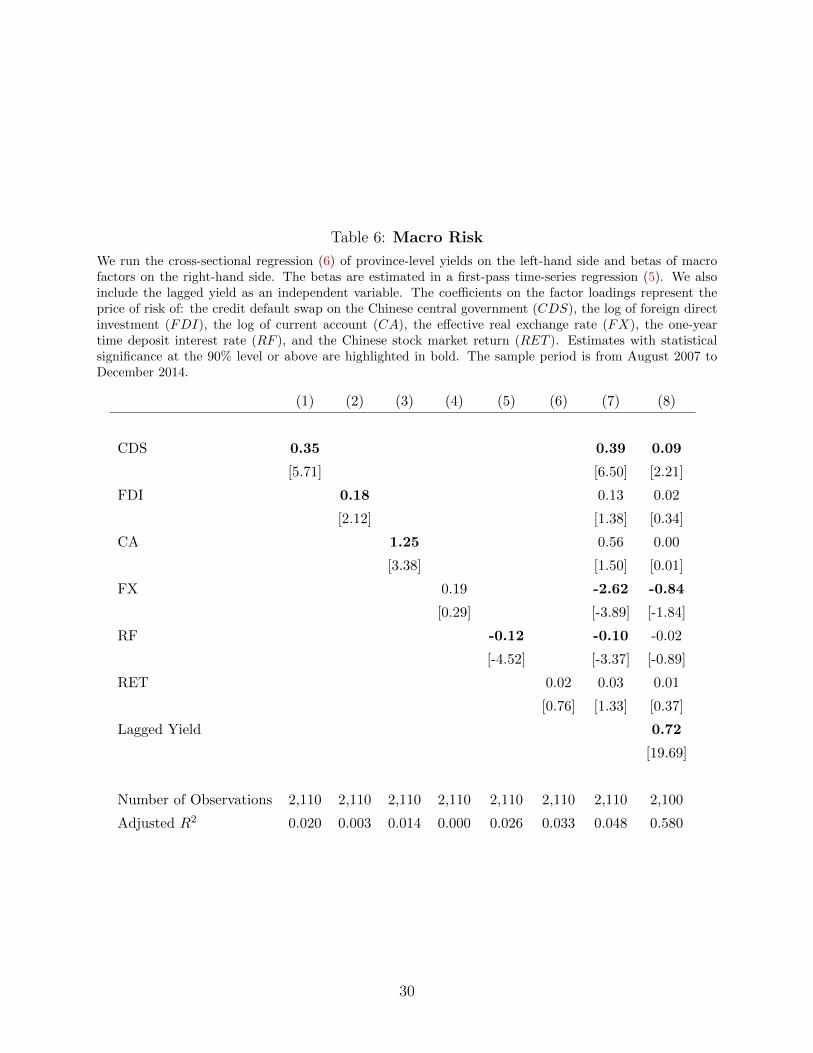
Table 6: Macro Risk

We run the cross-sectional regression (6) of province-level yields on the left-hand side and betas of macrofactors on the right-hand side. The betas are estimated in a first-pass time-series regression (5). We alsoinclude the lagged yield as an independent variable. The coefficients on the factor loadings represent theprice of risk of: the credit default swap on the Chinese central government (CDS), the log of foreign directinvestment (FDI), the log of current account (CA), the effective real exchange rate (FX), the one-yeartime deposit interest rate (RF ), and the Chinese stock market return (RET ). Estimates with statisticalsignificance at the 90% level or above are highlighted in bold. The sample period is from August 2007 toDecember 2014.

(1) (2) (3) (4) (5) (6) (7) (8)

CDS 0.35 0.39 0.09

[5.71] [6.50] [2.21]

FDI 0.18 0.13 0.02

[2.12] [1.38] [0.34]

CA 1.25 0.56 0.00

[3.38] [1.50] [0.01]

FX 0.19 -2.62 -0.84

[0.29] [-3.89] [-1.84]

RF -0.12 -0.10 -0.02

[-4.52] [-3.37] [-0.89]

RET 0.02 0.03 0.01

[0.76] [1.33] [0.37]

Lagged Yield 0.72

[19.69]

Number of Observations 2,110 2,110 2,110 2,110 2,110 2,110 2,110 2,100

Adjusted R2 0.020 0.003 0.014 0.000 0.026 0.033 0.048 0.580

30

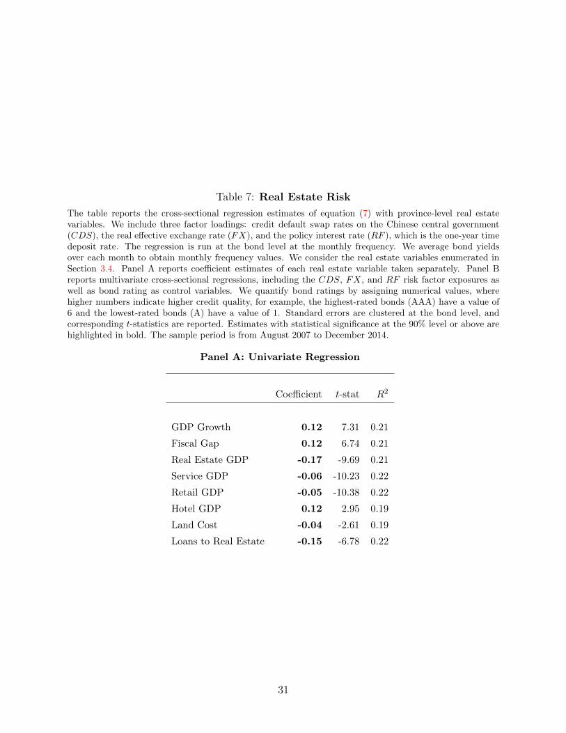
Table 7: Real Estate Risk

The table reports the cross-sectional regression estimates of equation (7) with province-level real estatevariables. We include three factor loadings: credit default swap rates on the Chinese central government(CDS), the real effective exchange rate (FX), and the policy interest rate (RF ), which is the one-year timedeposit rate. The regression is run at the bond level at the monthly frequency. We average bond yieldsover each month to obtain monthly frequency values. We consider the real estate variables enumerated inSection 3.4. Panel A reports coefficient estimates of each real estate variable taken separately. Panel Breports multivariate cross-sectional regressions, including the CDS, FX, and RF risk factor exposures aswell as bond rating as control variables. We quantify bond ratings by assigning numerical values, wherehigher numbers indicate higher credit quality, for example, the highest-rated bonds (AAA) have a value of6 and the lowest-rated bonds (A) have a value of 1. Standard errors are clustered at the bond level, andcorresponding t-statistics are reported. Estimates with statistical significance at the 90% level or above arehighlighted in bold. The sample period is from August 2007 to December 2014.

Panel A: Univariate Regression

Coefficient t-stat R2

GDP Growth 0.12 7.31 0.21

Fiscal Gap 0.12 6.74 0.21

Real Estate GDP -0.17 -9.69 0.21

Service GDP -0.06 -10.23 0.22

Retail GDP -0.05 -10.38 0.22

Hotel GDP 0.12 2.95 0.19

Land Cost -0.04 -2.61 0.19

Loans to Real Estate -0.15 -6.78 0.22

31

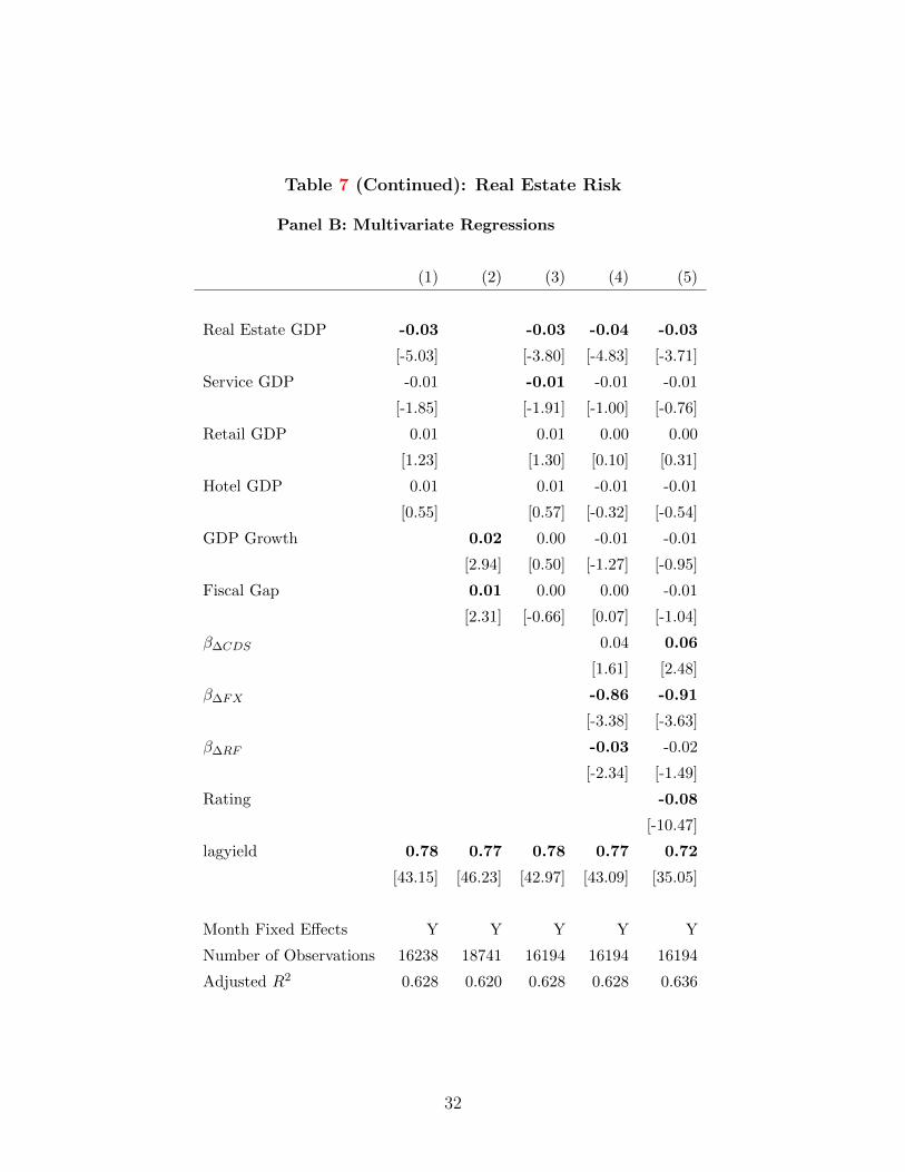
Table 7 (Continued): Real Estate Risk

Panel B: Multivariate Regressions

(1) (2) (3) (4) (5)

Real Estate GDP -0.03 -0.03 -0.04 -0.03

[-5.03] [-3.80] [-4.83] [-3.71]

Service GDP -0.01 -0.01 -0.01 -0.01

[-1.85] [-1.91] [-1.00] [-0.76]

Retail GDP 0.01 0.01 0.00 0.00

[1.23] [1.30] [0.10] [0.31]

Hotel GDP 0.01 0.01 -0.01 -0.01

[0.55] [0.57] [-0.32] [-0.54]

GDP Growth 0.02 0.00 -0.01 -0.01

[2.94] [0.50] [-1.27] [-0.95]

Fiscal Gap 0.01 0.00 0.00 -0.01

[2.31] [-0.66] [0.07] [-1.04]

β∆CDS 0.04 0.06

[1.61] [2.48]

β∆FX -0.86 -0.91

[-3.38] [-3.63]

β∆RF -0.03 -0.02

[-2.34] [-1.49]

Rating -0.08

[-10.47]

lagyield 0.78 0.77 0.78 0.77 0.72

[43.15] [46.23] [42.97] [43.09] [35.05]

Month Fixed Effects Y Y Y Y Y

Number of Observations 16238 18741 16194 16194 16194

Adjusted R2 0.628 0.620 0.628 0.628 0.636

32

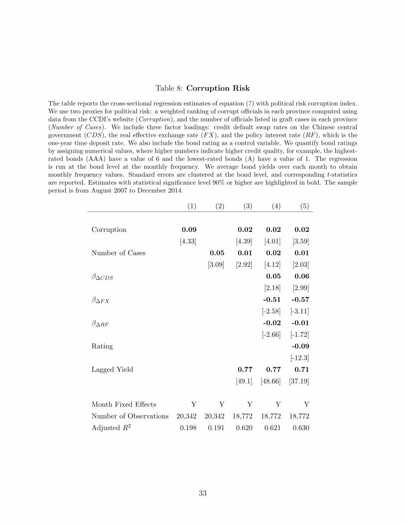
Table 8: Corruption Risk

The table reports the cross-sectional regression estimates of equation (7) with political risk corruption index.We use two proxies for political risk: a weighted ranking of corrupt officials in each province computed usingdata from the CCDI’s website (Corruption), and the number of officials listed in graft cases in each province(Number of Cases). We include three factor loadings: credit default swap rates on the Chinese centralgovernment (CDS), the real effective exchange rate (FX), and the policy interest rate (RF ), which is theone-year time deposit rate. We also include the bond rating as a control variable. We quantify bond ratingsby assigning numerical values, where higher numbers indicate higher credit quality, for example, the highest-rated bonds (AAA) have a value of 6 and the lowest-rated bonds (A) have a value of 1. The regressionis run at the bond level at the monthly frequency. We average bond yields over each month to obtainmonthly frequency values. Standard errors are clustered at the bond level, and corresponding t-statisticsare reported. Estimates with statistical significance level 90% or higher are highlighted in bold. The sampleperiod is from August 2007 to December 2014.

(1) (2) (3) (4) (5)

Corruption 0.09 0.02 0.02 0.02

[4.33] [4.39] [4.01] [3.59]

Number of Cases 0.05 0.01 0.02 0.01

[3.09] [2.92] [4.12] [2.03]

β∆CDS 0.05 0.06

[2.18] [2.99]

β∆FX -0.51 -0.57

[-2.58] [-3.11]

β∆RF -0.02 -0.01

[-2.66] [-1.72]

Rating -0.09

[-12.3]

Lagged Yield 0.77 0.77 0.71

[49.1] [48.66] [37.19]

Month Fixed Effects Y Y Y Y Y

Number of Observations 20,342 20,342 18,772 18,772 18,772

Adjusted R2 0.198 0.191 0.620 0.621 0.630

33

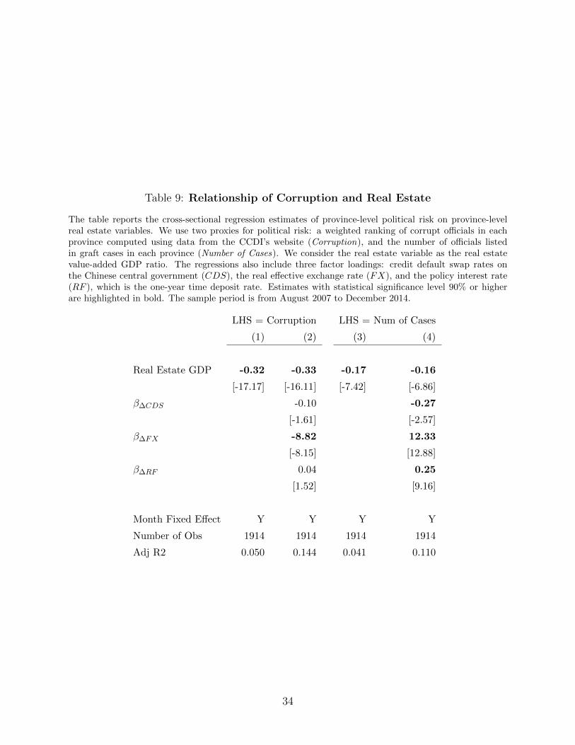
Table 9: Relationship of Corruption and Real Estate

The table reports the cross-sectional regression estimates of province-level political risk on province-levelreal estate variables. We use two proxies for political risk: a weighted ranking of corrupt officials in eachprovince computed using data from the CCDI’s website (Corruption), and the number of officials listedin graft cases in each province (Number of Cases). We consider the real estate variable as the real estatevalue-added GDP ratio. The regressions also include three factor loadings: credit default swap rates onthe Chinese central government (CDS), the real effective exchange rate (FX), and the policy interest rate(RF ), which is the one-year time deposit rate. Estimates with statistical significance level 90% or higherare highlighted in bold. The sample period is from August 2007 to December 2014.

LHS = Corruption LHS = Num of Cases

(1) (2) (3) (4)

Real Estate GDP -0.32 -0.33 -0.17 -0.16

[-17.17] [-16.11] [-7.42] [-6.86]

β∆CDS -0.10 -0.27

[-1.61] [-2.57]

β∆FX -8.82 12.33

[-8.15] [12.88]

β∆RF 0.04 0.25

[1.52] [9.16]

Month Fixed Effect Y Y Y Y

Number of Obs 1914 1914 1914 1914

Adj R2 0.050 0.144 0.041 0.110

34

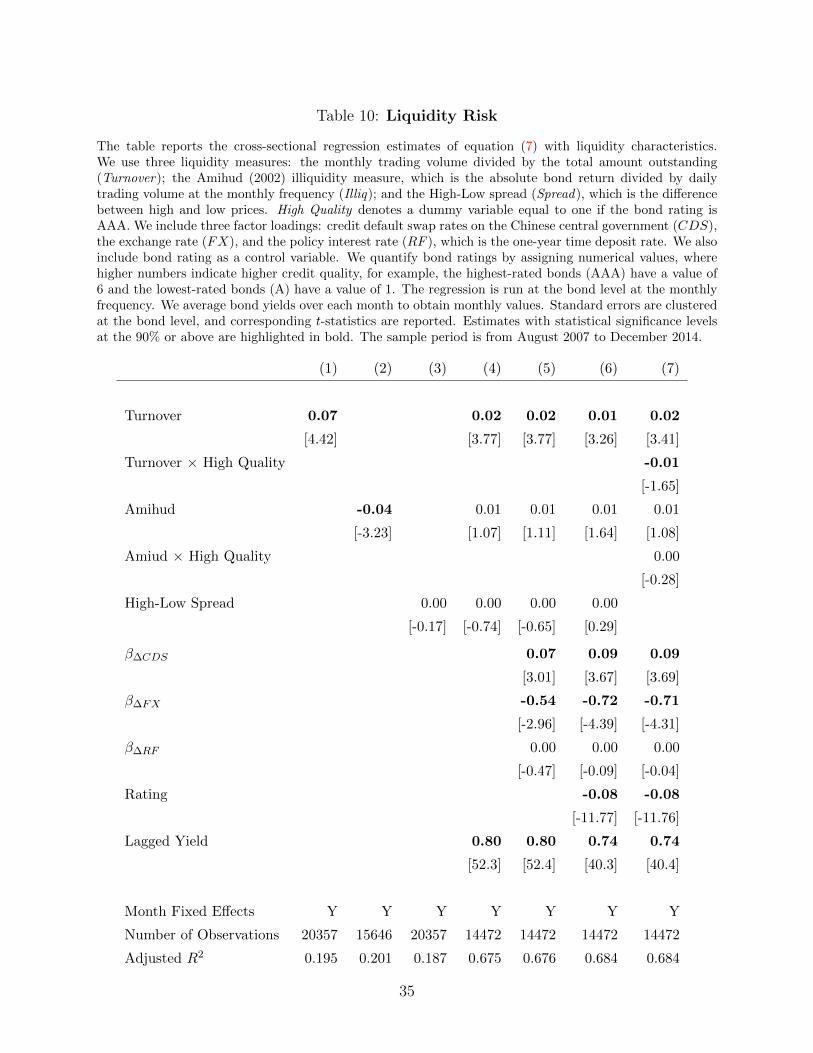
Table 10: Liquidity Risk

The table reports the cross-sectional regression estimates of equation (7) with liquidity characteristics.We use three liquidity measures: the monthly trading volume divided by the total amount outstanding(Turnover); the Amihud (2002) illiquidity measure, which is the absolute bond return divided by dailytrading volume at the monthly frequency (Illiq); and the High-Low spread (Spread), which is the differencebetween high and low prices. High Quality denotes a dummy variable equal to one if the bond rating isAAA. We include three factor loadings: credit default swap rates on the Chinese central government (CDS),the exchange rate (FX), and the policy interest rate (RF ), which is the one-year time deposit rate. We alsoinclude bond rating as a control variable. We quantify bond ratings by assigning numerical values, wherehigher numbers indicate higher credit quality, for example, the highest-rated bonds (AAA) have a value of6 and the lowest-rated bonds (A) have a value of 1. The regression is run at the bond level at the monthlyfrequency. We average bond yields over each month to obtain monthly values. Standard errors are clusteredat the bond level, and corresponding t-statistics are reported. Estimates with statistical significance levelsat the 90% or above are highlighted in bold. The sample period is from August 2007 to December 2014.

(1) (2) (3) (4) (5) (6) (7)

Turnover 0.07 0.02 0.02 0.01 0.02

[4.42] [3.77] [3.77] [3.26] [3.41]

Turnover × High Quality -0.01

[-1.65]

Amihud -0.04 0.01 0.01 0.01 0.01

[-3.23] [1.07] [1.11] [1.64] [1.08]

Amiud × High Quality 0.00

[-0.28]

High-Low Spread 0.00 0.00 0.00 0.00

[-0.17] [-0.74] [-0.65] [0.29]

β∆CDS 0.07 0.09 0.09

[3.01] [3.67] [3.69]

β∆FX -0.54 -0.72 -0.71

[-2.96] [-4.39] [-4.31]

β∆RF 0.00 0.00 0.00

[-0.47] [-0.09] [-0.04]

Rating -0.08 -0.08

[-11.77] [-11.76]

Lagged Yield 0.80 0.80 0.74 0.74

[52.3] [52.4] [40.3] [40.4]

Month Fixed Effects Y Y Y Y Y Y Y

Number of Observations 20357 15646 20357 14472 14472 14472 14472

Adjusted R2 0.195 0.201 0.187 0.675 0.676 0.684 0.684

35

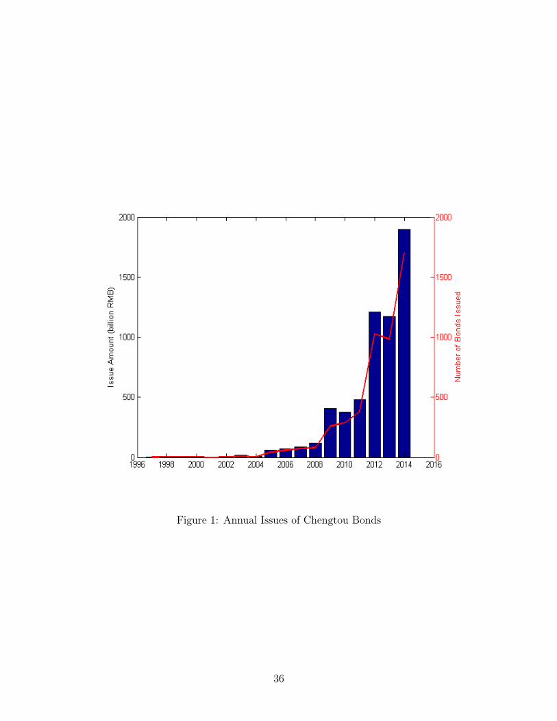
Figure 1: Annual Issues of Chengtou Bonds

36

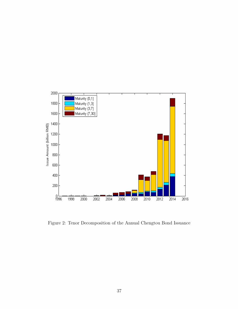
Figure 2: Tenor Decomposition of the Annual Chengtou Bond Issuance

37

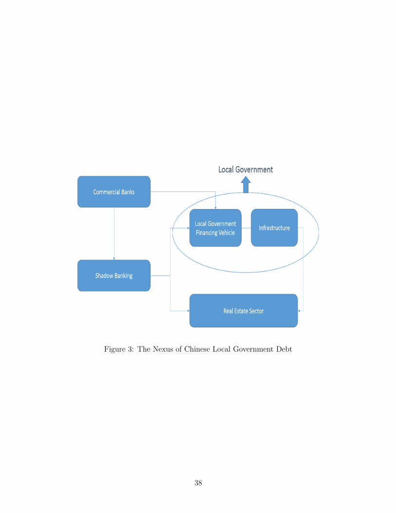
Figure 3: The Nexus of Chinese Local Government Debt

38

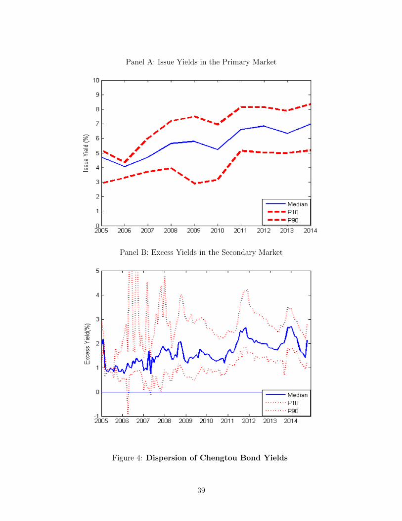
Panel A: Issue Yields in the Primary Market

Panel B: Excess Yields in the Secondary Market

Figure 4: Dispersion of Chengtou Bond Yields

39