NBER WORKING PAPER SERIES

THE GOVERNANCE AND PERFORMANCE OF RESEARCH UNIVERSITIES:EVIDENCE FROM EUROPE AND THE U.S.

Philippe AghionMathias DewatripontCaroline M. HoxbyAndreu Mas-Colell

André Sapir

Working Paper 14851http://www.nber.org/papers/w14851

NATIONAL BUREAU OF ECONOMIC RESEARCH1050 Massachusetts Avenue

Cambridge, MA 02138April 2009

We gratefully acknowledge funding for the survey of European universities from Bruegel, a Europeanthink tank based in Brussels, supported by European governments and private corporations. For theirassistance with the university survey, we are very grateful to Aida Caldera, Indhira Santos, and AlexisWalckiers. For comments on this work, we thanks Charles Clotfelter, Paul Courant, and Ronald Ehrenberg.The views expressed herein are those of the author(s) and do not necessarily reflect the views of theNational Bureau of Economic Research.

© 2009 by Philippe Aghion, Mathias Dewatripont, Caroline M. Hoxby, Andreu Mas-Colell, and AndréSapir. All rights reserved. Short sections of text, not to exceed two paragraphs, may be quoted withoutexplicit permission provided that full credit, including © notice, is given to the source.

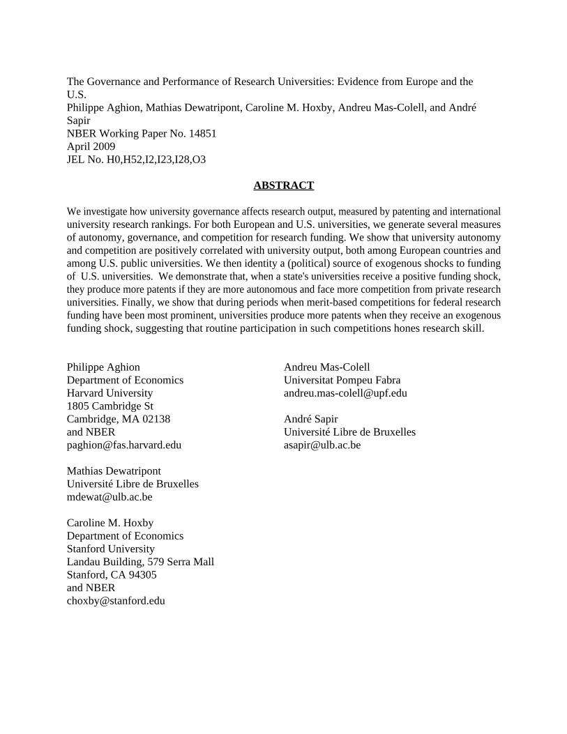
The Governance and Performance of Research Universities: Evidence from Europe and theU.S.Philippe Aghion, Mathias Dewatripont, Caroline M. Hoxby, Andreu Mas-Colell, and AndréSapirNBER Working Paper No. 14851April 2009JEL No. H0,H52,I2,I23,I28,O3

ABSTRACT

We investigate how university governance affects research output, measured by patenting and internationaluniversity research rankings. For both European and U.S. universities, we generate several measuresof autonomy, governance, and competition for research funding. We show that university autonomyand competition are positively correlated with university output, both among European countries andamong U.S. public universities. We then identity a (political) source of exogenous shocks to fundingof U.S. universities. We demonstrate that, when a state's universities receive a positive funding shock,they produce more patents if they are more autonomous and face more competition from private researchuniversities. Finally, we show that during periods when merit-based competitions for federal researchfunding have been most prominent, universities produce more patents when they receive an exogenousfunding shock, suggesting that routine participation in such competitions hones research skill.

Philippe AghionDepartment of EconomicsHarvard University1805 Cambridge StCambridge, MA 02138and NBERpaghion@fas.harvard.edu

Mathias DewatripontUniversité Libre de Bruxellesmdewat@ulb.ac.be

Caroline M. HoxbyDepartment of EconomicsStanford UniversityLandau Building, 579 Serra MallStanford, CA 94305and NBERchoxby@stanford.edu

Andreu Mas-ColellUniversitat Pompeu Fabraandreu.mas-colell@upf.edu

André SapirUniversité Libre de Bruxellesasapir@ulb.ac.be

Harvard University, Bruegel, CEPR†

Université Libre de Bruxelles††

Stanford University and NBER†††

University Pompeu Fabra††††

Université Libre de Bruxelles, Bruegel, CEPR†††††

1

The Governance and Performance of ResearchUniversities: Evidence from Europe and the U.S.

P. Aghion , M. Dewatripont , C. Hoxby, A. Mas-Colell , & A. Sapir† †† ††† †††† †††††

December 2008

1 Introduction

With increasing globalization has come increasing scrutiny of the differences

in the performance of countries' universities. Such performance differences

are thought to be especially important for advancing science, technology, and

the industries that depend upon them. Thus, it is not surprising that when

Shanghai University and other organizations began to publish indices of

university output, the indices garnered a great deal of attention. Although

such indices are undoubtedly flawed and focus on science, to the exclusion of

social sciences, the arts, and even the applied sciences, they highlight

apparently massive differences in the output of different countries'

universities. Some European policy makers see in the indices a potential

explanation for their countries' disappointing economic growth. This is not an

unreasonable deduction because the growth of technology-intensive industries

has been particularly disappointing in Europe compared to the United States

(U.S.) and some other countries. U.S. universities are obvious positive outliers

in performance on the international indices. At present, several European

countries are considering reforms to their university systems that would make

them more like those of the U.S. Beyond the anecdotal evidence just

mentioned, there is, however, little factual basis for the claim that if non-U.S.

universities modeled themselves on American ones, they would produce

similar output. Furthermore, what aspects of American universities deserve

imitation? Surely not all.

This paper attempts to fill this evidentiary gap. Specifically, we

hypothesize that more autonomous universities that need to compete more for

resources are more productive. These hypotheses--autonomy and competition--

are intertwined both in practice and logically. There is little point and possibly

some danger in giving universities great autonomy if they are not in an

2

environment disciplined by competition for research funding, faculty, and

students. There is little point in promoting competition among universities if

they do not have sufficient autonomy to respond with more productive,

inventive, or efficient programs. (We recognize that autonomy and competition

are separate concepts and--to the extent we can--we attempt to distinguish

them empirically. Because they are intertwined in practice, however, we

investigate them as something of a package.)

Why do we hypothesize that autonomy and competition, in combination,

may improve universities' output? First, we are guided by economic logic. In

higher education, the production function is very hard for outsiders to observe.

In research, government policy makers are unlikely to understand the

production function even if they could observe it. Under such circumstances,

centralized government control may be much less effective, as a form of

governance, than making largely autonomous organizations compete with one

another for resources and prizes. Second, we are guided by correlations. In

the next section, we show that universities' performance is correlated with

their autonomy and competitive environment. Within Europe, we show that

some countries, such as the United Kingdom (U.K.) and Sweden, have

unusually autonomous universities and unusually productive universities. For

the U.S., we show that states' public universities differ considerably in their

autonomy and the degree to which they face local competition from private

universities. We find that universities' output is higher in the states in which

they are more autonomous and face more competition. Third, certain facts

about U.S. universities direct us away from explanations other than autonomy

and competition. Highly regarded international assessments suggest that

primary and secondary education in the U.S. is mediocre at best compared to

its developed country counterparts. Thus, U.S. universities' success is unlikely

to be due to the better preparation of their incoming students. Many of the

highest performing U.S. universities are private and therefore receive, by

international standards, only very modest guaranteed government funding.

If U.S. universities' success is due purely to greater government support, the

mechanism by which this happens is obscure. (Private universities do compete

for federal research grants but they otherwise receive minimal and only

indirect financial help from the government--mostly in the form of grants to

students they enroll.)

In Section 2, we conduct the correlational analysis just described, using the

well-known Shanghai University ranking of world universities as our measure

of universities' output. The Shanghai index aggregates information on

publications, citations, and honors such as Nobel Prizes and Field Medals. We

recognize that science and math are overrepresented in the measures on which

the Shanghai index is based, but we accept this bias partly because policy

makers who draw a link between higher education and their economies are

especially interested in science and engineering. There are no existing

measures of European universities' governance, so we surveyed university

leaders, asking questions such as "Does your university's budget need to be

3

approved by the state?" and "What percentage of your university's budget

depends on grants for which you must compete?" For the U.S., we cull similar

measures from administrative sources and existing surveys. An advantage of

the U.S. data is that we can measure governance as far back as the 1950s. Our

main findings in Section 2 are that universities with higher Shanghai rankings

enjoy greater autonomy and draw a higher percentage of their budgets from

competitive resources.

The correlations shown in Section 2 are merely suggestive. They do not

necessarily indicate that university autonomy and competition cause higher

output. Reverse causality is quite plausible: Perhaps governments allow very

productive universities to be more autonomous and such universities campaign

for resources to be allocated by competition, rather than rules. Omitted

variables could also be a problem. For instance, universities may enjoy

resources and forms of government support that we do not observe. The

universities with the greatest difficult-to-observe resources may also enjoy

greater autonomy and "win" more research competitions (which could be

stacked in their favor).

In Sections 3 and 4, we turn to causal analysis. Specifically, we test

whether universities produce more output from an exogenous increase in their

resources if they are more autonomous and face more competition. This is

(nearly) a sufficient condition for autonomy and competition to cause greater

university output. (We say "nearly" because we can only test what universities

produce with marginal resources, and it is always possible that they use

marginal resources efficaciously and inframarginal resources inefficaciously

or vice versa.) Although we would like to conduct causal analysis for Europe,

we rely on U.S. states for this part of the analysis. We do this because, first,

we have 1950s measures of universities' governance and competition from

private institutions. Since the 1950s are just the beginning of the modern era

of higher education, especially research university funding, the early measure

allows us to greatly limit the potential for reverse causality. Second, we have

found instruments that generate exogenous variation in funding for U.S.

universities. These instruments depend on vacancies arising on legislative

committees in the U.S. and the convoluted processes by which the vacancies

are filled. The instruments are fairly complicated and are discussed below and

elsewhere (Aghion, Boustan, Hoxby, and Vandenbussche, 2006; hereafter

ABHV). The bottom line is that (i) the vacancy filling process generates

variation in government funding for universities and (ii) the vacancy filling

process is so remote from other phenomena that affect universities that we

believe that it could affect them only through the funding channel. Third, we

have 25 years of panel data on U.S. states that include university

expenditures, higher education administrative data, and patents. Patents

measure universities' output in a way that is substantially broader and more

closely linked to technology and the economy than the Shanghai measure. Our

main findings in Section 4 are that exogenous increases in expenditures of U.S.

universities generate more patents if the universities in question are more

We cannot do full justice to the literature on education and growth, especially as1

it is tangential to this paper. However, we recommend Acemoglu (2009) and Aghionand Howitt (2009) as fairly comprehensive introductions to the work.

See Jaffe (1989), Adams (2002), Anselin, Varga, and Acs (1997), Vargas (1998),2

and Fischer and Varga (2003) for studies of the local economic effects of universityresearch.

4

autonomous and face more local competition (for resources, faculty, and

students) from private universities.

In Section 5, we note that the stakes in U.S. research competitions have

varied greatly over time. In some periods, more than $20 billion of federal

research money has been at stake annually. In other periods, the federal

award stakes have been only $1 to $5 billion annually. Since the stakes have

risen and fallen in a highly nonmonotonic way, we can differentiate the effect

of an environment rich in research competitions from other time trends. Our

main finding is that the effects of research universities' expenditures,

autonomy, and competition are all elevated in periods of high stakes

competition for federal awards.

We draw upon several related literatures. Most obviously, we draw upon

the large existing literature on university governance. Nearly all of this

literature is descriptive, and we rely on it for our understanding of how to

measure autonomy. Our 1950s measure of university autonomy is drawn from

the report of a national commission on the subject that produced an

informative book by Moos and Rourke (1959). Only a few studies attempt to

estimate the relationship between universities' governance and their

performance--most notably, Volkwein (1986) and Volkwein et al (1997 and

1998). Our question is somewhat inspired by the existing, vast literature on

education and growth, but that literature's connection to this paper is tenuous

because it tends to use aggregate measures of education (such as average years

attained). That literature does not differentiate education investments by type

or expenditure, and it certainly does not differentiate them by governance of

schools. 1

This paper shares instruments and some data with ABHV, but the focus

is entirely different. The one theoretical idea we borrow from ABHV (and the

more seminal Acemoglu, Aghion, and Zilibotti, 2006) is that investments in

research-type education should pay off most in areas that are close to the world

technological frontier because such areas specialize in innovation.2

Conversely, we expect investments in vocational and lower types of education

to pay off most in areas below the technological frontier because such areas

specialize in imitation. Sapir et al (2003) use the same approach to argue that

European countries need to invest more in higher, as opposed to vocational,

education to attain growth rates typical of the U.S. In any case, these ideas

motivate us to allow the effect of an exogenous increase in education

expenditure to vary with proximity to the technological frontier.

For our understanding of the politics behind our instruments, we are

5

indebted to the previous literature on the politics of committee selection and

its consequences--mostly importantly, Masters (1961), Rohde and Shepsle

(1973), Bullock (1985), Munger and Torrent (1993), Stewart and Groseclose

(1999), Hedlund and Patterson (1992), Squire (1988), Hedlund (1989), and

Payne (2003). For our understanding of patents as a measure of research

outcomes, we are indebted to the previous literature on patenting, especially

Hall, Jaffe, and Tratjenberg (2001) and Hall (2006).

2 Correlations between University Autonomy and UniversityOutputIn this section, we show that measures of university autonomy are correlated

with measures of university output. We also show that universities that need

to compete for research funding tend to have higher output. We offer this

evidence as suggestive--that is, it suggests the hypotheses that we test with

analysis that is more credibly causal, in the next section.

2.1 The Shanghai Ranking of World Universities

In 2003, Shanghai Jiao Tong University began publishing an "Academic

Ranking of World Universities" (2008). It is now the best known measure of

universities' output and it puts weight on six indices, as follows:

1. The number of alumni from the university who have won Nobel Prizes in

physics, chemistry, medicine, or economics or Field Medals in mathematics

(10% of the overall index);

2. The number of faculty of the university who have won Nobel Prizes in

physics, chemistry, medicine, or economics or Field Medals in mathematics

(20% of the overall index);

3. The annual number of articles authored by faculty of the university that are

published in the journals Nature or Science (20% of the overall index);

4. The annual number of articles authored by faculty of the university that are

in the Science Citation Index-expanded and Social Science Citation Index (20%

of the overall index);

5. The number of Highly Cited Researchers (copyright Thomson ISI, 2008) in

the university's faculty in 21 broad subject categories (20% of the overall

index);

6. All of the above indicators divided by the number of full-time equivalent

faculty (10% of the index).

Obviously the choice of criteria and the weights on them are quite

arbitrary. They are also heavily weighted toward science. However, the

arbitrariness is less problematic that it might seem because, in fact, the

available measures that one could reasonably put into any index of university

output are highly correlated. For instance, each of the components of the

Shanghai index is highly correlated with each other component. Also, the

Shanghai index is highly correlated with two rankings that use different

methodology: the Times Higher Education - QS World University Ranking

(2008) and with the Webometrics Ranking of World Universities (2008). In

An approximate number can be computed using the methodology described by3

Shanghai Jiao Tong University. We need to do this for two American universities: theUniversity of South Dakota and the University of North Dakota. These are the mainresearch universities of two U.S. states with very small populations.

The bar labeled "U.S.-sized continental Europe" includes Germany, France, the4

Netherlands, Italy, Sweden, Switzerland, Belgium, Denmark, Spain, and Austria.

6

short, we make no claims for the correctness of the Shanghai rankings but use

it because it is widely known and--more importantly--is based on criteria that

are themselves reasonable measures of output and correlated with other

reasonable measures of output.

The world's highest ranked university is given the number 1 and so on

down to number 100. After that, universities' ranking are indicated by a

numerical range--"101 to 151," for example. Universities below 500 are not

given a number. We invert the rankings throughout this section so that the3

university with the highest number is the highest ranked university.

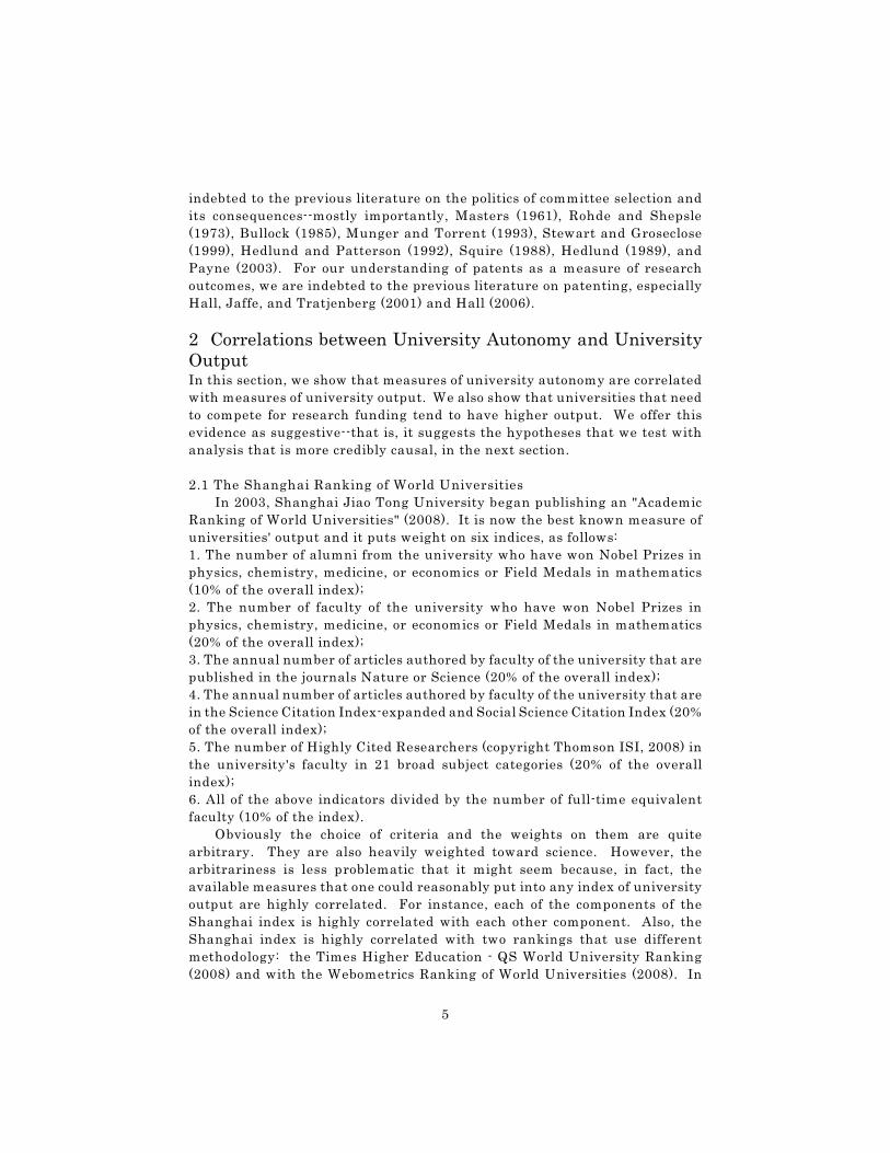
Simply to provide a sense of the numbers to which policy makers around

the world are reacting, we show in Figure 1 the sum of top-500 Shanghai

rankings of universities in each country. Clearly, the U.S. has the highest sum

of rankings and the next nearest country, the U.K., has only one quarter as

many. Of course, much of the apparent U.S. dominance is due simply to its

population. (For instance, Canada and the U.K. do slightly better than the

U.S. on a per-person basis.) There is no perfect way to correct for population

since it is not obvious that the effect of population should be linear. However,

one comparison that may be useful is adding up the countries of continental

Europe that have the highest sums of rankings until their population is equal

to that of the U.S. This procedure (which favors Europe because it selects its4

areas on university output but does not do the same for the U.S.) generates the

bar labeled as"U.S.-sized continental Europe." This area, with the same

population as the U.S., generates a sum of Shanghai rankings that is only 62

percent as large.

Japanese universities also do not compare favorably to U.S. universities.

To see this, consider that Japan's sum of rankings is 5,934, which is 92 percent

of the sum of rankings of the state of California. Japan's population is 3.5

times that of California.

Overall, Figure 1, which we see as a very crude indicator only, suggests

that U.S., U.K., and Canadian universities have higher output than

continental European or Japanese universities. Since the U.S., U.K., and

Canadian universities share some institutional and legal history, this crude

evidence points us towards explanations, such as governance, that are

systemically related to history. Note also that there is important variation in

output within Europe. We explore this in a moment.

Below, where we correlate the interesting variation in Shanghai indices

with governance variables, we use individual university data. We thus

alleviate the problem of accounting for population since each country and U.S.

Bruegel is a European think tank based in Brussels. Its acronym stands for5

European and Global Economic Laboratory, and it is supported by Europeangovernments and leading private corporations. For their assistance with the universitysurvey, we are very grateful to Aida Caldera,Indhira Santos, and Alexis Walckiers.

7

state, with the possible exception of a few, can support one research university

at scale. Most countries and states voluntarily have multiple such universities.

2.2 A Survey of European Universities

Because no measures of governance existed for European universities, we

surveyed the 196 European universities with Shanghai rankings in the top

500. The survey was generously supported by Bruegel and is described in

greater detail in Aghion, Dewatripont, Hoxby, Mas-Colell, and Sapir (2007 and

2008). These universities are spread across 14 countries and vary5

substantially in their age, public versus private control, number of students,

and the relative importance of various disciplines (medicine, law, natural

sciences, and so on).

In fall 2006, we sent a questionnaire to university leaders. Among the

survey questions were several related to autonomy, competition, and

governance more generally. We asked (paraphrasing for succinctness):

• Does the university set its own curriculum?

• Does the university select its own students or is there centralized

allocation?

• To what extent does the university select its own professors?

• How much does the state intervene in setting wages?

• Are all professors with the same seniority and rank paid the same wage?

• Does the university's budget need to be approved by the government?

• What share of the university's budget comes from core government

funding?

• What share comes from research grants for which the university must

compete?

We also ask what percentage of the university's professors have their doctoral

degrees from the university itself. A high number on this measure, endogamy,

suggests that hiring is not open.

It is important to understand that, in surveying European universities, we

were mainly attempting to record differences in governance between countries

and not within countries. Countries typically have legal and institutional rules

within which their universities function. It is this set of rules that we wish to

The response rate did vary among countries, as shown in Appendix Table 1.6

There are several possible explanations for this including institutional arrangementsand the cultural reaction to external surveys.

Median answers reveal similar patterns.7

8

describe. We are less interested in whether a particular university gets special

treatment (perhaps because of its history) or how a particular university leader

interpreted the questions. In short, we are mainly concerned with whether the

survey respondents were representative of their countries.

On this criterion, the survey worked well. While only 71 (36 percent) of the

surveyed universities responded, the universities that responded within any

given country had rankings that were representative of the country's whole

population of universities.6

Appendix Table 1 shows the average answer on individual survey

questions that are relevant to this paper, for several European countries. The7

table confirms that there is a wide variety in countries' institutional and

governance arrangements. For instance, the share of universities that must

get their budgets approved by the government varies from lows of 0 and 13

percent in Denmark and the U.K., respectively, to highs of 100 percent in

Finland, France, and Germany. The share of universities that report that

their baccalaureate students are selected via a centralized mechanism, rather

than by the university acting on its own, ranges from lows of 0 in Finland and

France and 12 percent in the U.K. to highs of 83 percent in Spain and 100

percent in Ireland. In five countries (Belgium, Denmark, Finland, Sweden,

and the U.K.), faculty may be paid different amounts even if they have

identical seniority and rank. On the other hand, at least half the universities

in countries like France, Italy, Spain, and Switzerland report that they must

pay the same amount to faculty with the same seniority and rank. These same

countries (with the exception of Switzerland) are likely to report that their

hiring is not mainly controlled internally. Endogamy, which suggests that a

country is not open to hiring from the outside, is greater than 50 percent in

Belgium, France, Spain, and Sweden. However, we ought to be cautious about

interpreting endogamy because it may also reflect the willingness of foreigners

to live in a country, teach and write in that country's language, and so on. For

instance, endogamy is low in Germany and the U.K. (and dramatically lower

in the U.S.) partly because German and English are useful lingue francae.

2.3 Similar Measures for U.S. Universities

Rather than surveying U.S. universities ourselves, we use a combination

of administrative data and existing surveys to derive similar variables for

American states. We have a response rate of 100 percent on all variables we

use. This is probably because American universities believe that they must

respond to information requests, even if they are not official requests from the

government. This is because not responding is perceived as a lack of

willingness to inform prospective faculty and students. (In other words, the

9

high response rates are probably endogenous to the competition for resources,

faculty, and students.) We attempt to obtain a U.S. measure that is the

parallel for every European measure described in Appendix Table 1. However,

the parallel measures are not constructed identically. This is fine for our

purposes because we mean to compare governance among U.S. states, not

between the U.S. and European countries. We reserve most details of our

sources and variable construction for the Data Appendix.

From now on, we describe a U.S. state's governance environment by (i) its

percentage of universities that are private and (ii) autonomy and competition

variables that describe the rules for its public universities. We do not bother

to describe autonomy and competition variables for private U.S. universities

because the distributions would be degenerate. For instance, all American

private universities do not seek budget approval from the government, do

control selection of their students, do control faculty hiring and salaries, do

own their own buildings, and do get a negligible share of their budget from

core government funds.

In the 1950s, the governance of public universities in the U.S. was studied

by a national commission, the Committee on Government and Higher

Education. They produced the three 1950s autonomy variables on which we

rely: a university's freedom from centralized purchasing, a university's

freedom from needing to get its budget approved, and a university's freedom

to hire and pay personnel (not merely faculty but also staff) without

government control or the need to follow civil service pay rules. All of these

measures are category responses intended to measure degree of autonomy, not

yes/no responses. There are separate measures for a state's research/doctoral

universities and its 4-year and 2-year colleges.

2.4 Correlations between University Output and an Overall Measure of

University Autonomy and Control

We begin by doing factor analysis on our European measures of autonomy

and competition, the corresponding (modern) measures for U.S. public

universities, and our three 1950s measures of U.S. public university autonomy.

We do not include the percent of universities that are private in the factor

analysis but, instead, use this as a separate variable. The factor analysis

includes variables that are best thought of as proxies for autonomy (for

instance, whether the budget needs to be approved by the state) and best

thought of as proxies for the competitive environment (the percentage of the

budget from research grants for which the university must compete). Yet, in

practice, the variables loads on a single principal factor in all three analyses.

Put another way, there is some autonomy and competition "package" on which

universities vary in the data. Universities do not vary on autonomy and then

vary independently on competition. If they did, we would obtain at least two

principal factors.

The autonomy factor for European universities is maximized for

universities that (i) do not need to seek government approval of their budget,

Universities in the U.S. are classified by the Carnegie Foundation for the8

Advancement of Teaching (2005) into several categories, which include research,doctoral, various types of mainly baccalaureate-granting institutions, and two-yearcolleges. The basic classification is long-standing and uncontroversial.

10

(ii) select their baccalaureate students in a manner independent of the

government, (iii) pay faculty flexibly rather than based on a centralized

seniority/rank-based scale, (iv) control their hiring internally, (v) have low

endogamy, (vi) own their own buildings, (vii) set their own curriculum, (viii)

have a relatively low percentage of their budget form core government funds,

and (ix) have a relatively high percentage of their budget from competitive

research grants.

The factor loadings for the U.S. autonomy index based on recent data are

similar except that the building ownership and curriculum setting variables

are not used because they are degenerate--that is, all public colleges and

universities in the U.S. report that they set their own curriculum and own

their own buildings.

The factor loadings for the U.S. autonomy index based on 1950s data are

such that the index is maximized for colleges/universities that report that their

purchasing is entirely independent of centralized control, that they need not

seek approval of their budget, and that they completely control personnel

hiring and pay.

We normalize the first principal factor (hereafter, the "autonomy index"

since most of our variables are best thought of as proxies for autonomy) to have

a mean of zero and a standard deviation of one.

Figure 2 contains a scatterplot and fitted regression line that show that a

European university's Shanghai ranking is correlated with its autonomy index.

(The size of the circles varies with a university's size because we are

attempting to describe the averages for countries and a size-weighted

regression is therefore appropriate.) Observe that U.K. universities are

clustered in the upper right corner, having both high autonomy indices and

high rankings. Swedish universities also generally appear in the upper, right

quadrant. Spain's universities are clustered in the lower left corner, having

both low autonomy indices and low rankings. The remaining countries'

universities are somewhere in the middle. The correlation is such that a

standard deviation in European university autonomy is associated with 78.5

rank points on the Shanghai index (moving past 78.5 universities, in other

words).

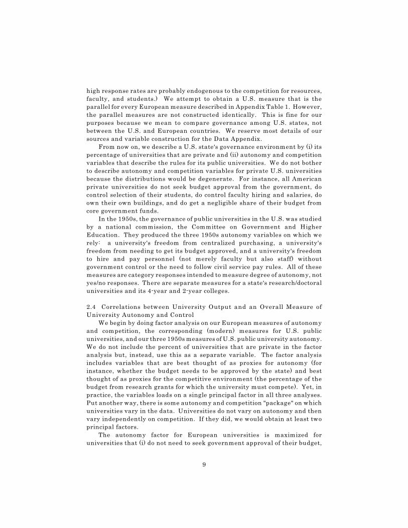
Figure 3 shows a similar scatterplot for U.S. states with an autonomy

index based on recent data for public research/doctoral universities. Each8

state is represented by its top-ranked public university because the autonomy

index describes the environment for them. States with high rankings and high

autonomy include Washington, Colorado, Hawaii, Delaware, California,

Maryland, Wisconsin, Minnesota, and Michigan. States with low rankings and

low autonomy include Arkansas, South Carolina, Louisiana, Kansas, Idaho,

11

South Dakota, and Wyoming. The last two are states with very small

populations, but the other states in this group are large enough to support a

public research university. The correlation is such that a standard deviation

in U.S. public research/doctoral university autonomy is associated with 50.3

rank points on the Shanghai index.

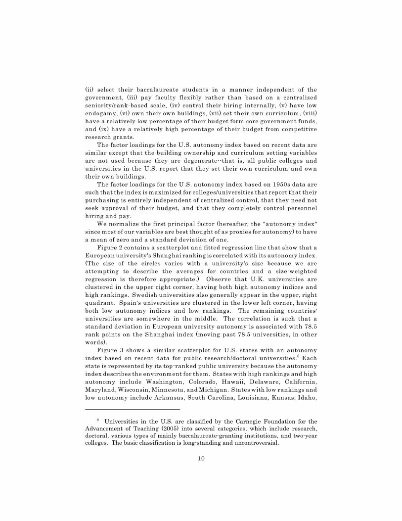
Finally, Figure 4 shows the same data except that the autonomy index

reflects the autonomy of public research/doctoral universities in the 1950s.

The correlation is such that a standard deviation in 1950s public

research/doctoral university autonomy is associated with 38.7 rank points on

the Shanghai index. Although the 1950s index is based on entirely different

variables gathered in a quite different way, there are noticeable commonalities

between Figure 4 and the previous figure. Once again, we see that states like

California, Colorado, Minnesota, Wisconsin, and Michigan have high rankings

and high university autonomy. We see that low rankings and low autonomy

again characterize Arkansas, South Carolina, Louisiana, Kansas, Idaho, South

Dakota, and Wyoming (as well as some other states). In other words, although

the 1950s and recent autonomy measures are not identical, they clearly reflect

institutional arrangements that resist change. Such persistent differences in

governance probably reflect the idiosyncratic origins of American universities.

For instance, Thomas Jefferson, the founder of the University of Virginia,

himself set some aspects of the university's relationship with the state. (In fact,

based on our reading of the extensive literature on university governance, we

believe that the empirical differences between 1950s and recent autonomy

measures overstate the actual changes in governance within each state. Much

the difference between the 1950s measure and recent measure is probably due

to the fact that they based on variables that were gathered using quite

different methodologies.)

Of course, none of the correlations that we have shown so far are evidence

that having greater autonomy/competition causes a university to have higher

output. Figure 4, which relates recent output rankings to 1950s autonomy

makes the possibility of strict reverse causality remote, but the possibility

remains that both the rankings and autonomy are caused by some third factor

which does not change much over time within a state.

2.5 Correlations between University Output and Individual Indicators of

University Autonomy and Control

Let us now examine correlations with output for a few of the most

interesting individual proxies for university autonomy and control. (The

variables we examine were all elements in the factor analysis.)

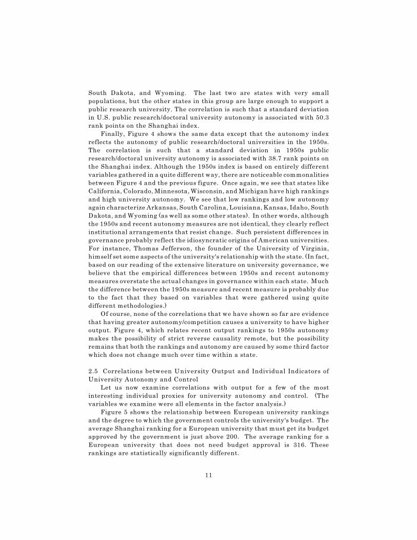
Figure 5 shows the relationship between European university rankings

and the degree to which the government controls the university's budget. The

average Shanghai ranking for a European university that must get its budget

approved by the government is just above 200. The average ranking for a

European university that does not need budget approval is 316. These

rankings are statistically significantly different.

12

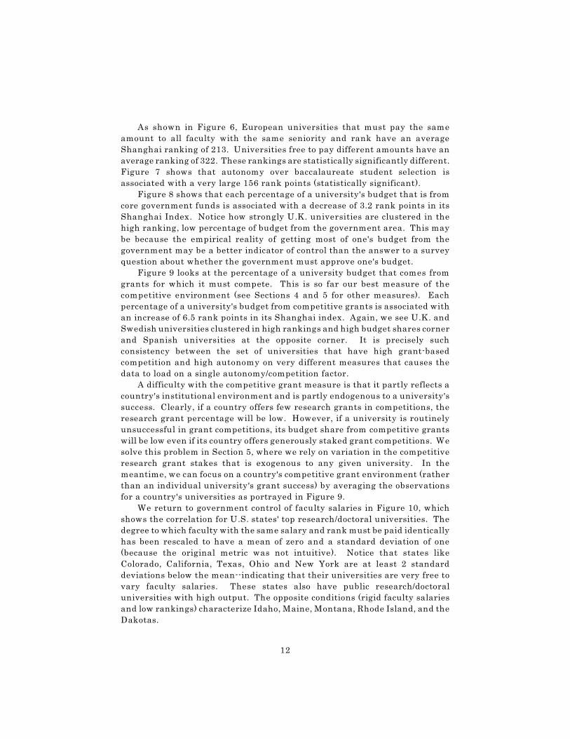
As shown in Figure 6, European universities that must pay the same

amount to all faculty with the same seniority and rank have an average

Shanghai ranking of 213. Universities free to pay different amounts have an

average ranking of 322. These rankings are statistically significantly different.

Figure 7 shows that autonomy over baccalaureate student selection is

associated with a very large 156 rank points (statistically significant).

Figure 8 shows that each percentage of a university's budget that is from

core government funds is associated with a decrease of 3.2 rank points in its

Shanghai Index. Notice how strongly U.K. universities are clustered in the

high ranking, low percentage of budget from the government area. This may

be because the empirical reality of getting most of one's budget from the

government may be a better indicator of control than the answer to a survey

question about whether the government must approve one's budget.

Figure 9 looks at the percentage of a university budget that comes from

grants for which it must compete. This is so far our best measure of the

competitive environment (see Sections 4 and 5 for other measures). Each

percentage of a university's budget from competitive grants is associated with

an increase of 6.5 rank points in its Shanghai index. Again, we see U.K. and

Swedish universities clustered in high rankings and high budget shares corner

and Spanish universities at the opposite corner. It is precisely such

consistency between the set of universities that have high grant-based

competition and high autonomy on very different measures that causes the

data to load on a single autonomy/competition factor.

A difficulty with the competitive grant measure is that it partly reflects a

country's institutional environment and is partly endogenous to a university's

success. Clearly, if a country offers few research grants in competitions, the

research grant percentage will be low. However, if a university is routinely

unsuccessful in grant competitions, its budget share from competitive grants

will be low even if its country offers generously staked grant competitions. We

solve this problem in Section 5, where we rely on variation in the competitive

research grant stakes that is exogenous to any given university. In the

meantime, we can focus on a country's competitive grant environment (rather

than an individual university's grant success) by averaging the observations

for a country's universities as portrayed in Figure 9.

We return to government control of faculty salaries in Figure 10, which

shows the correlation for U.S. states' top research/doctoral universities. The

degree to which faculty with the same salary and rank must be paid identically

has been rescaled to have a mean of zero and a standard deviation of one

(because the original metric was not intuitive). Notice that states like

Colorado, California, Texas, Ohio and New York are at least 2 standard

deviations below the mean--indicating that their universities are very free to

vary faculty salaries. These states also have public research/doctoral

universities with high output. The opposite conditions (rigid faculty salaries

and low rankings) characterize Idaho, Maine, Montana, Rhode Island, and the

Dakotas.

13

Figure 11 shows that, for each percentage of a public research/doctoral

university's budget that comes from core public funds, its rank decreases by 2.7

points. However, this amount is too small to be statistically significant

different from zero. In contrast, the relationship between output and

dependence on competitive grants is large in magnitude and statistically

significant. Each percentage of a public university's budget that depends on

competitive grants is associated with 5.4 rank points on the Shanghai index.

Keep in mind, however, that the competitive grant measure is problematic

because it is somewhat endogenous to a university's success. This is addressed

in Section 5.

2.6 Summing Up the Correlational Evidence

Universities' autonomy and competition, which appear in practice as

something of a package, are clearly related to universities' output. It remains

to be seen whether the relationship is causal. We draw confidence from the

similarity of the correlational evidence from Europe and the U.S. Despite

differences in institutions, laws, culture, and our data gathering methods,

there are clear commonalities such as salary inflexibility and a university's

need for government budget approval being negatively correlated with output.

3 An Empirical Strategy for Obtaining Credibly CausalEvidence on the Effects of Autonomy and Competition

Suppose that a more autonomous university with a greater need to

compete for resources makes better use of every dollar of funding. Then,

greater autonomy and greater competition would generate higher output all

else equal. In other words, a sufficient condition for autonomy and competition

generating greater performance is that they enhance the return to any given

investment in the university. We would like to test this sufficient condition.

We cannot do so in a strict sense because there are dollars of funding that are

always inframarginal and therefore do not vary so that we could test their

returns. However, we can test the output generated by exogenous changes in

marginal funding, and this is what we do in this section.

How do we identify exogenous variation in universities' funding?

Subsection 3.2 explains the political instruments that we use. They are the

most important element of our empirical strategy.

3.1 The Basics

Apart from the instruments, our estimation strategy is a fairly transparent

attempt to estimate, in reduced-form, how a state's 1950s autonomy index, its

percentage of universities that are private, and its proximity to the technology

frontier affect the number of patents it produces for a given expenditure on

education. In simplified form:

Thursby, Fuller, and Thursby (2007) show that university researchers sit a top9

a network of industry researchers who generate patents related to their scholarlyresearch.

14

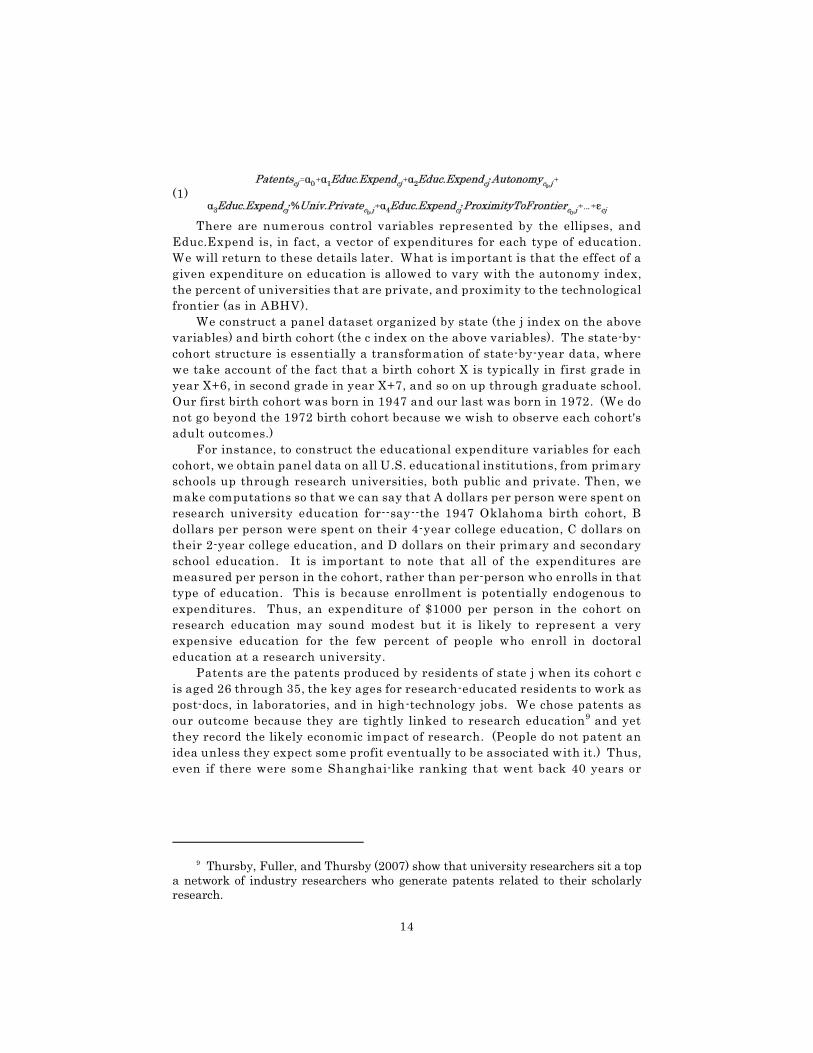
(1)

There are numerous control variables represented by the ellipses, and

Educ.Expend is, in fact, a vector of expenditures for each type of education.

We will return to these details later. What is important is that the effect of a

given expenditure on education is allowed to vary with the autonomy index,

the percent of universities that are private, and proximity to the technological

frontier (as in ABHV).

We construct a panel dataset organized by state (the j index on the above

variables) and birth cohort (the c index on the above variables). The state-by-

cohort structure is essentially a transformation of state-by-year data, where

we take account of the fact that a birth cohort X is typically in first grade in

year X+6, in second grade in year X+7, and so on up through graduate school.

Our first birth cohort was born in 1947 and our last was born in 1972. (We do

not go beyond the 1972 birth cohort because we wish to observe each cohort's

adult outcomes.)

For instance, to construct the educational expenditure variables for each

cohort, we obtain panel data on all U.S. educational institutions, from primary

schools up through research universities, both public and private. Then, we

make computations so that we can say that A dollars per person were spent on

research university education for--say--the 1947 Oklahoma birth cohort, B

dollars per person were spent on their 4-year college education, C dollars on

their 2-year college education, and D dollars on their primary and secondary

school education. It is important to note that all of the expenditures are

measured per person in the cohort, rather than per-person who enrolls in that

type of education. This is because enrollment is potentially endogenous to

expenditures. Thus, an expenditure of $1000 per person in the cohort on

research education may sound modest but it is likely to represent a very

expensive education for the few percent of people who enroll in doctoral

education at a research university.

Patents are the patents produced by residents of state j when its cohort c

is aged 26 through 35, the key ages for research-educated residents to work as

post-docs, in laboratories, and in high-technology jobs. We chose patents as

our outcome because they are tightly linked to research education and yet9

they record the likely economic impact of research. (People do not patent an

idea unless they expect some profit eventually to be associated with it.) Thus,

even if there were some Shanghai-like ranking that went back 40 years or

Patent data are easy to use at the state-by-year level (which we do) but10

cumbersome to trace back to universities. Patents are associated with a year, thepatentee's name, and the patentee's state of residence. While some scholars havetraced patents back to their origins in university research by studying patentees'academic origins and careers, such studies are practical only for small numbers ofpatents. We use all utility patents in all states over 36 years--far too many for auniversity trace-back analysis but ideal for a state-by-cohort analysis.

15

more, as patent data do, we would still prefer patent data to ranking data.10

All three of the interaction variables are recorded as early as possible--

1957 for the autonomy index, 1960 for percentage of universities that are

private, and 1960 for proximity to the frontier. We then interact only these

0earliest recorded levels, which is why the variables are indexed by c in the

equation. We use only the earliest recorded levels because we wish to avoid

reverse causality that might occur if, for instance, a state's patenting success

moved it closer to the frontier, induced the government to give its universities

more autonomy, and so on. All of our early-recorded interaction variables

greatly predate the era in which our earliest birth cohort (1947) could possibly

have themselves affected patents, public university autonomy, the percentage

of universities that are private, or proximity to the technological frontier.

The percentage of colleges and universities that are private is self-

explanatory. We have already described the autonomy index: the first

principal factor from a factor analysis of the Moos and Rourke (1959)

governance variables. Note that we interact the autonomy index for research

universities with research university expenditures and the autonomy index for

4-year and 2-year colleges with those colleges' expenditures.

Proximity to the technological frontier can be measured in one of a few

ways, all of which tend to produce similar results. Here we use per worker

labor earnings in the state divided by per worker labor earnings in the state

with the highest such earnings. Proximity to the frontier thus tops out at 1.

In practice, the states furthest from the frontier have proximity of about 0.5.

To ensure that we do not confound our variables of interest with state-

specific omitted variables that are fairly constant across time, time-specific

omitted variables that are fairly constant across states, or state-specific time

trending variables, all of our estimations control for a full set of state indicator

variables, cohort indicator variables (equivalent to year indicator variables),

and state-specific linear time trends. These are some of the variables

represented in the ellipses in equation (1). The remaining variables

represented by the ellipses are political, and the need for them will become

clear when the instruments are explained.

3.2 Instrumental Variables for Educational Expenditures

We need instrumental variables for educational expenditures because it is

likely that they are simultaneously determined with other outcomes for a state

and time. Most worrisome would be some unknown, third factor (not captured

Another location-specific earmark is funding for a military base in the11

legislator's constituency. However, only a small minority of legislators havesufficiently large military bases in their constituencies to consider this a usefulearmark. There are of course many tiny earmarks that are possible--funding for aspecific theater restoration or local social program. However, such earmarks simplydo not have the capacity to deliver funds in quantity as do research projects andinfrastructure projects.

16

by time effects or state-specific linear time trends) that cause a state to invest

more in education over time and also become more inventive. For instance, if

there were an exogenous increase in the demand for inventive goods, people

might be induced to engage in more patenting and policy-makers might be

inclined to support more educational expenditures, simply because they

believed that education caused invention (even if it did not).

As instruments, we require variables that shift educational expenditures

among states and over time in arbitrary ways unrelated to other determinants

of patenting. We find such instruments in the politics of legislative committee

assignment. It is easiest to illustrate how the instruments work by starting

with an example for federal educational expenditures, all of which are directed

to research universities.

In the U.S. House of Representatives and Senate, the Appropriations

Committees control the allocation of federal funds to projects. Most research

funds for universities are awarded through a competitive process, so that the

Appropriations Committees simply allocate the a lump sum to agencies like

the National Science Foundation. The agencies then disburse the money

using merit-based research competitions. However, the Appropriations

Committees can also propose that certain individual projects be funded

without regard to merit or larger policy considerations. These are called

earmarks. It is well known that congressmen use earmarks to pay back their

constituents for support, resulting in so-called pork-barrel spending. A seat on

the Appropriations Committee is valuable precisely because it allows a

congressperson to deliver pay back to his constituents. Now, many forms of

spending are formula-based and are, therefore, inefficient ways to channel

spending to one's constituents. For instance, a congressmen may have

numerous Medicare recipients (elderly people who rely on the federally-funded

medical plan), but it would not be efficient for him to pay them back by raising

Medicare spending. This is because he could only increase the generosity of the

Medicare formula, and most of the increased generosity would go to people

outside his constituency. There are only couple of ways that most legislators

can send money to their constituency and only their constituency. The first is

earmarking funds for research at an institution located in the constituency.

The second is earmarking funds for a particular bridge or similar

infrastructure project located in the constituency. ABHV provide case studies11

of particular legislators who, upon becoming Appropriations committee

members, directed billions of dollar to research universities in their

17

constituency, building laboratories, medical schools, and other research

facilities.

Because a seat on the Appropriations Committee is so valuable, a legislator

who has one does not give it up voluntarily. Both houses of Congress respect

an incumbent committee member's right to continue on this committee. Thus,

once on, a legislator tends to stay on the committee for several years, and

nearly all vacancies arise because a member has died in office or retired from

legislative political life (through old age or being appointed, say, to the

President's cabinet). In any case, a vacancy sets off a complex political process

that generates our instruments. Although the process is not written down

formally, political scientists and our own work have determined the implicit

process to be roughly as follows. When a vacancy arises, each party (Democrat

and Republican) considers the resulting state composition of the committee

within its party and whether that composition matches the state composition

of its party members in its house of Congress. Thus, if when the vacancy

occurs, Florida's Democratic legislators occupy 5 percent of the Democratic

committee places but Florida Democrats make up 10 percent of the Democrats

in the house, Florida has a representation gap of 5 percent. The state with the

largest gap is very likely to fill the vacancy, and political custom is such that

the most senior, eligible legislator from the state is very likely to be the new

committee member. (To be eligible, a legislator must not be on the committee

already or occupying a high ranking seat on one of a couple of other very

powerful committees.) Now, if vacancies arose very regularly (for instance, if

legislators never served more than one term), then the state and party

composition of the Appropriations Committee would always be a mirror image

of the Congress. But, in fact, incumbent legislators (especially multi-term

incumbents) usually win elections in the U.S. because campaign finance, the

drawing of election districts, and other phenomena make them likely to defeat

challengers in an election. Since an incumbent legislator keeps his seat on the

committee, the committee can become very imbalanced over time. For

instance, consider Massachusetts, which shifted from being a bi-partisan state

to a mostly Democratic state. It had a couple of incumbent Republican

legislators on the Appropriations Committee. As its party preferences shifted,

these incumbents kept their committee seats even while the Democratic party-

-through the process described above--was obliged to appoint Massachusetts

Democrats to the committee. Thus, Massachusetts ended up with much more

representation on the Appropriations committee than the state's population

warranted. Of course, for every lucky state like Massachusetts that is in the

right place at the right time and becomes overrepresented, there is an unlucky

state that becomes underrepresented.

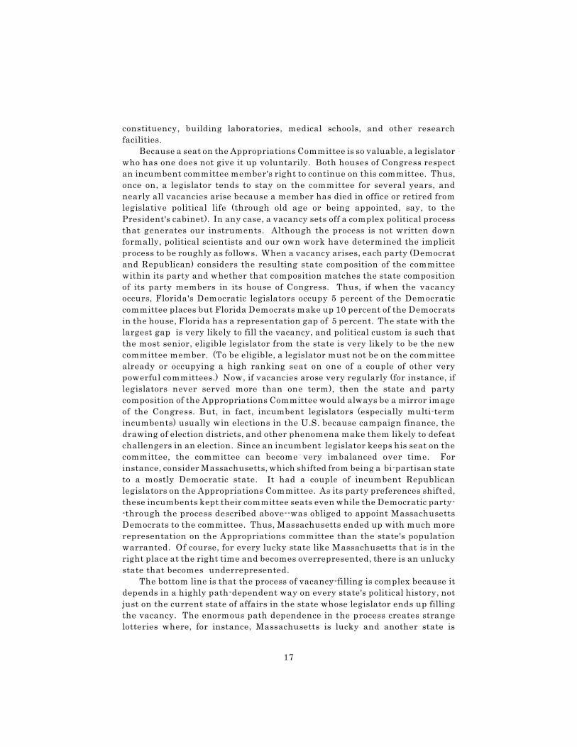
The bottom line is that the process of vacancy-filling is complex because it

depends in a highly path-dependent way on every state's political history, not

just on the current state of affairs in the state whose legislator ends up filling

the vacancy. The enormous path dependence in the process creates strange

lotteries where, for instance, Massachusetts is lucky and another state is

State senates often do not have separate appropriations and finance committees,12

but have a single committee that performs both the spending and the taxationfunctions .

18

unlucky. Thus, our instruments--which are the interaction between the arrival

of a vacancy and within-party state gap in committee membership at the

moment the vacancy arises--generate variation in states' representation on the

Appropriations Committee and, consequently, variation in federal funding for

states' educational institutions. It is not plausible that, through some other

channel, these instruments directly affect the tendency of the state's residents

to generate patents.

The federal instruments just described provide the crucial, arbitrary

shocks to the expenditure of research universities. (Remember that these

arbitrary funds are in addition to whatever the research universities might

earn through merit-based competitions for federal funding.) However, federal

funds are sent only to research universities, not 4-year or 2-year colleges.

Thus, we need different instruments for them. We turn to the politics of state

legislatures since it is they that determine government funding for 4-year and

2-year colleges. We again exploit the arrival of vacancies on legislative

committees--this time the chairmanships of the state senate's appropriations

and education committees. We rely on changes in the higher education12

institutions that are located in the chairman's constituency when that

chairmanship changes hands. This is best illustrated with an example.

Suppose that state senator X whose constituency included a public 4-year

college retires from chairing his senate's appropriations or education

committee. Suppose that he is replaced by a senator whose constituency

includes a public 2-year college. Empirically, we see government funding shift

from government funding from 4-year colleges to funding for 2-year colleges.

The next time a vacancy arises, we see another shift, perhaps away from

college education altogether and toward entirely different spending areas--this

outcome is likely if the new senator's constituency includes no colleges. We do

not claim that it is random that a senator is made a committee chairman, but

we do not think that the change in the specific colleges located in the

chairman's constituency is likely affect patenting except through the channel

of chairman-generated shocks to state funding for specific colleges. To be

precise, our instruments are the number of enrolled students at each type of

college (public 4-year, private 4-year, public 2-year, private 2-year) in the

chairman's constituency. We use 1960 enrollment (the earliest available) for

all cohorts. Thus, the instruments change only because the chairman changes.

They do not reflect the ongoing success of a college, something that could be

endogenous to a chairman's generosity with public funds.

We have asserted that our political instruments do not reflect

contemporary federal or state politics in such a way that they might affect

patents through a channel other than expenditure. But, is our assertion true?

We test it by controlling for several variables designed to pick up contemporary

19

politics, both for state elections to federal positions and for local elections to

state positions. These include the Democratic vote share of a state's delegation

to Congress over the period a cohort would normally pursue doctoral

education, the Democratic vote share for a state's legislature over the period

a cohort would normally pursue 4-year college education, the same vote share

over the period a cohort would normally pursue 2-year college education, and

the same vote share over the period a cohort would normally pursue primary

and secondary education. We also include parallel variables for the

Independent vote share--that is, the share of votes for candidates who are

neither Democrats nor Republicans.

We control for primary and secondary educational expenditure but do not

have good instruments for it. We therefore strongly discourage the reader

from interpreting its coefficient in a causal way.

3.3 Summarizing and Extending the Empirical Strategy

We are now in a position to summarize our empirical strategy. Intuitively,

we see whether an arbitrary expenditure shock to a state's research university

funding, 4-year college funding, or 2-year college funding has an effect on a

state's patenting over the period when the cohort who receives the shocks is

most likely to be contributing to professional research that generates economic

returns. We see whether that effect varies with the autonomy of the state's

institutions of higher education, the state's percentage of colleges and

universities that are private, and the state's proximity to the technological

frontier. Because the political circumstances that generate the shocks tend to

last about six years, a cohort may experience the full impact of a shock or only

part of one.

Formally, we identify the effects of educational expenditures on patenting

from within state, within-time, within-state-linear-time-trend variation. Using

instruments, we identify the local effects of variation in expenditure generated

by variables that predict Appropriations Committee membership (federal funds

for research university expenditure) or variables that describe the colleges in

the constituencies of state senate chairmen of appropriations or education

committees. We control for contemporary politics. We estimate robust

standard errors clustered at the state level to account for the fact that adjacent

birth cohorts have overlapping educational experiences.

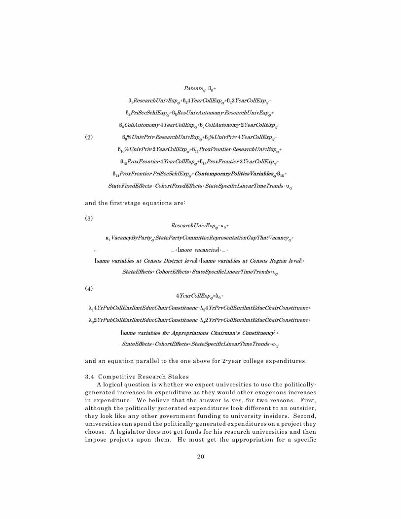
In equations, this strategy's main (second-stage) specification is:

20

(2) ;

and the first-stage equations are:

(3)

,

(4)

,

and an equation parallel to the one above for 2-year college expenditures.

3.4 Competitive Research Stakes

A logical question is whether we expect universities to use the politically-

generated increases in expenditure as they would other exogenous increases

in expenditure. We believe that the answer is yes, for two reasons. First,

although the politically-generated expenditures look different to an outsider,

they look like any other government funding to university insiders. Second,

universities can spend the politically-generated expenditures on a project they

choose. A legislator does not get funds for his research universities and then

impose projects upon them. He must get the appropriation for a specific

21

project that the university itself proposes. Third, and perhaps most important,

the politically-generated expenditures we study are large enough to generate

interesting variation but they are not large relative to inframarginal spending.

Thus, if a university is in the habit of spending research funds efficaciously,

it is likely to spend the exogenous increase efficaciously, and vice versa.

We take account of this last fact to test whether research universities use

their exogenous increases in expenditure better if, for their inframarginal

research funds, they need to compete in high stakes, merit-based competitions.

The stakes in research fund competitions vary with the total size of the "pot"

established by the federal government. We show below that this varies

substantially and nonmonotonically over time. To test whether the stakes

matter, we estimate a version of equation (2) in which the research university

expenditure variables are interacted with the federal competitive research

stakes for the relevant years.

4 The Effects of Autonomy and Competition on the Output froma Given Educational Expenditure

Descriptive statistics for the variables we use in our estimation may be found

in Appendix Table 2. Notes to our tables also provide key information on data

sources. However, the data sources for and creation of our instrumental

variables are so numerous and complex that we refer the reader to the Data

Appendix.

Table 1 presents the main results of the causal analysis: the coefficients

from estimating equation (2) by instrumental variables. Because the equation

includes several interaction terms that, in practice, covary, it is best to focus

on the signs of coefficients, rather than their magnitudes, when reading the

table. We use figures to interpret the magnitude of the coefficients.

The three top rows of the table show that the main effects of expenditures

on research universities, 4-year colleges, and 2-year colleges are respectively

negative, negative, and positive at zero autonomy, zero percent of universities

private, and zero proximity to the technological frontier. However, the

minimum value of proximity is 0.5. Therefore, the negative signs of the first

coefficients should simply be taken as a indication that it is possible to waste

money on research universities and 4-year colleges. If a state were to spend

funds on them without regard to their governance or the need for their output,

the state would presumably discourage real economic activity and probably

discourage patenting as well.

The coefficients of the variables interacted with the autonomy index are of

primary interest. (Note that the main effect of the autonomy index does not

appear because the index is constant within a state over time and is therefore

absorbed by the state indicator variable.) Recalling that the autonomy index

has mean zero and standard deviation 1 by construction, we see that research

universities with above average autonomy generate more patents for any given

22

expenditure. Similarly, 4-year colleges with above average autonomy cause

more patents for any given expenditure. Autonomy apparently does not

improve the effect of 2-year colleges on patents. This may be because, unlike

research and baccalaureate education, vocational higher education generates

imitative patents--that is, patents that make some practical adaptation to an

existing technology. Such patent may benefit from standardization,

centralized state purchasing, and so on. The essential difference is that, in

order to produce inventions at the frontier, research education needs to be

creative, somewhat speculative, and perhaps beyond the ken of state

regulators.

Next, consider the coefficients of the variables interacted with the

percentage of universities that are private. (The main effect of percent private

is absorbed by the state indicator variable.) The percentage of universities

that are private has mean 0.19 and standard deviation 0.24. We see that the

existence of local private colleges and universities, which presumably fosters

competition between the private and public sectors, makes private research

universities generate more patents for any given expenditure. It also makes

4-year colleges generate more patents for any given expenditure. It has the

opposite effect on 2-year colleges, perhaps because they end up competing with

private vocational schools that have low standards. Poorly managed 2-year

private schools in U.S. are a perennial concern.

Finally, the coefficients indicate that, as expected, proximity to the frontier

makes the effect of expenditures on patents greater for research and 4-year

education but has the opposite effect on 2-year college education. As in ABHV,

the logic of this is that areas close to the frontier are likely to generate

technological innovations if research education increases. In contrast, areas

far from the frontier will most likely generate imitative patents (practical

adaptations of existing technologies) and such patents may be promoted most

by 2-year college education.

It is very difficult to interpret the coefficients in Table 1 in a manner that

tells us much about policy. This is because the three interaction variables

covary significantly. Thus, if we want to understand the implications of the

results, it is best to show what they imply for actual states. We show these

implications in Figures 13, 14, and 15. To construct each figure, we take each

state's actual value of each interaction variable and we multiply it by the

appropriate coefficient and then sum all the products. For instance, to

generate the Alabama bar in Figure 13, we multiply Alabama's autonomy

index by 0.029, multiply its percent private universities by 0.110, and multiply

its proximity to the frontier by 0.242. We then add these products to the base

coefficient of -0.173. By doing this for every U.S. state, we hope to give readers

a sense of the likely range of effects of educational expenditures on patenting.

Figure 13 shows that half of the states generate more patents when

expenditure on their research universities increases. The states that generate

the most patents per dollar of exogenous expenditure are those with high

university autonomy, a high percentage of universities that are private, and

23

close proximity to the frontier. In New Jersey, for instance, $1000 in research

university expenditure per person in the cohort increases patenting by

residents of that state by 0.146 standard deviations. The estimated effects are

also high for California, Illinois, Massachusetts, Maryland, Michigan,

Minnesota, Missouri, New Hampshire, New York, Vermont, and Wisconsin.

(It should mentioned that Massachusetts and New Hampshire may be

somewhat conflated because the belt of high technology jobs in the outskirts

of Boston, Massachusetts spills over into southern New Hampshire.) In

contrast, it appears that expenditures on research universities do not increase

(or possibly even decrease) patenting in states with low university autonomy,

a low percentage of universities that are private, and considerable distance

from the frontier: Alabama, Arkansas, Kansas, Kentucky, New Mexico,

Nevada, Oregon, South Carolina, and West Virginia. We should emphasize

that all of these predictions contain error so that policy makers should not take

their own state's coefficient very seriously. (Their state might be anomalous.)

However, one can take seriously the overall range of effects, from very positive

in states like New Jersey to a waste of expenditure in states that do not have

university autonomy, competition from private universities, or close proximity

to the frontier. While a policy maker might not be able to change his state's

proximity, he could make changes to the autonomy of public universities and

promote competition between his states' public universities and other

institutions.

Figure 14 shows that the vast majority of states generate more patents

when expenditure on their 4-year colleges increases. Nevertheless, the size of

the positive effect varies substantially. The states that generate the most

patents per dollar of exogenous expenditure are those with high university

autonomy, a high percentage of universities that are private, and close

proximity to the frontier. For instance, a $1000 increase in 4-year college

expenditure per person in the cohort would increase patenting by residents

0.130 of a standard deviation in California and about 0.10 of a standard

deviation in Connecticut, Florida, Illinois, Massachusetts, Maryland, New

Jersey, and New York. The effect of the same $1000 increase in 4-year college

expenditure would likely not increase (and might even decrease) patenting in

states like Alabama, Arkansas, Maine, and a few others. It is important to

understand that $1000 of expenditure on 4-year college education per person

in the cohort is likely to be spread more evenly among colleges than is $1000

on research education per person in the cohort. Thus, it is not surprising that

the range of effects for 4-year college expenditure is smaller among states than

the range of effects for research university expenditure. The latter effects

depend far more on a few (or even just one) research universities.

Figure 15 shows that about half of the states generate more patents when

expenditure on their 2-year colleges increases. States with the biggest positive

effects are those far from the technological frontier. States with the biggest

negative effects are those close to the technological frontier. The coefficients

also suggest that lower autonomy and a lower percent private make a state's

24

2-year college expenditures generate more patents. However, the autonomy

and percent private effects are tiny, whereas the effect of proximity is massive.

Proximity to the frontier essentially accounts for the entire pattern seen in

Figure 15: autonomy and percent private do not matter much for 2-year

college expenditures.

The estimated effects shown in Table 1 are not sensitive to a number of

changes in the specification. For instance, if any one or even two of the

interaction variables is dropped from the equation, the coefficients retain the

same signs (although magnitudes of course change because of the covariance

among interaction variables). Excluding the contemporary political variables

has essentially no effect on the coefficients, which is what we expect if the

instruments are legitimate. Shifting to a different measure of proximity to the

frontier also has little effect on the coefficients. All these results are available

from the authors.

Summing up, it appears that public university autonomy and local

competition from private institutions cause research universities and 4-year

colleges to produce more output, measured in patents, for given increase in

expenditure. This strongly suggests that the correlations we saw between

university output and measures of autonomy in Section 2 were in fact the

expression of a causal relationship. If the relationships are causal, as we

would now like to suggest, then policy makers are not without options. They

can improve the output of their research universities and baccalaureate

institutions by giving them greater autonomy and making them compete for

resources, faculty, and students. However, the results for states far from the

technological frontier tell a cautionary tale. Giving autonomy to and

introducing competition among institutions of higher education may be

ineffective in countries far from the technological frontier.

5 Competition for Research Grants

If very little money is attached to merit-based competitions for research grants,

universities are unlikely to invest much in preparing for such competitions.

If the funds associated with winning a competition are small, universities may

find that there are easier ways to get funds than delivering the most promising

project. For instance, a university might prefer to spend its effort courting

politicians. Thus, we expect that when the stakes of research grant

competitions are greater--that is, when universities' funding depends more on

their performance in these competitions--universities will invest in preparation

that allows them to make better use of research funds. We attempt to test this

hypothesis in this section.

Figure 16 shows federal research and development obligations through the

three agencies that dominate the merit-based competitions in which

universities compete: the National Science Foundation, the National

The source is National Science Foundation (2008). Although other agencies,13

such as the Department of Defense, also have large research and developmentobligations, most of their obligations go to private firms or contractors who produceproducts that will ultimately be sold to the government.

25

Institutes of Health, and the National Aeronautics and Space Administration.13

We see in Figure 16 that the stakes of federal merit-based grant competitions

were negligible from 1951 through about 1960. There was thereafter a boom

in the stakes of such competitions, with the late 1960s being the high water

mark: $23 billion real dollars per year at the peak. The stakes fell from this

peak until 1982, when they were just over $5 billion in real dollars. Since

then, the stakes have risen (with the notable exception of the year 2000) to

about $12 billion in real dollars. Fortunately, this time pattern for the stakes

is so nonmonotonic that it could not be confounded with any number of other

trends that affect research universities, such as private philanthropy, rising

incomes, and the like. Therefore, we believe that we can test the effect of

higher stakes in research competitions on how productively universities use

exogenous increases in funding. Intuitively, if a university is in the habit of

preparing research projects well because it needs to win competitions, does

that university make better use of an exogenous increase in research funding?

Table 2 shows results of estimating a version of equation (2) in which

research university expenditures are interacted with the stakes in federal

competitions for research grants. The stakes are also interacted with

expenditures times autonomy and with expenditures times percent private.

(The main effects of the federal stakes are absorbed by the cohort fixed effects.)

Again, focus on signs; we use a figure to interpret magnitudes. Higher stakes

make research university expenditures generate a greater number of patents,

all else equal. Higher stakes also improve the effects of autonomy and

improve the effects of a higher percent private. All these coefficients are highly

statistically significant. These results suggest that autonomy and market

competition improve universities' research output more when those

universities can see that research effort is richly rewarded through merit-

based competitions. In other words, policy makers may have a role to play by

focusing universities' competition on research, as opposed to politics or other

activities. Universities are induced to use their autonomy productively when

they operate in a high stakes, competitive research environment.

Figure 17 is intended to help with the interpretation of magnitudes.

Figure 17 is essentially the same as Figure 13--it shows the effect on patents

of $1000 of expenditure by research universities in various states. However,

in Figure 17, we show the effects for stakes of $10 billion and $16 billion. $10

billion is close to the average for federal research competition over our

estimation period. $16 billion is two standard deviations above that average.

It may be seen that an exogenous increase in research universities'

expenditure has a much greater effect on patenting when the stakes are $16

billion than when they are $10 billion. For instance, in California,

In Aghion et al (2008), we argue that, whatever one may think about student14

fees, they are a potentially important source of revenue for European universities.While U.S. institutions of higher education have revenue equal to 3.3 percent of U.S.GDP, European universities' revenue is only equal to 1.3 percent of European GDP.

26

Massachusetts, and New Jersey, the effect on patenting more than triples.

Before concluding that higher stakes in research competitions improve the

output of universities, we need to sound a note of caution. We have not tried

to explain why the stakes varied over time as they did. While most of the

popular explanations, such as the American desire to match Russia's Sputnik

space craft, would probably not affect our interpretation, we would be

concerned if we knew that the federal government raised the stakes when it

knew that research was likely to produce patents and lowered the stakes when

it knew that research was unlikely to do so. However, since we have argued

all along that governments do not know much about frontier research (this is

why they run competitions rather than simply telling universities what to do),

it seems unlikely the federal government would know enough to raise and

lower the stakes with the year's potential for invention.

6 Lessons for Europe

Our causal analysis on U.S. data strengthens the conclusions we draw from the

correlational evidence on both Europe and the U.S.: Autonomy and competition

enhance the impact of university funding on research. Our results therefore

provide support for policies that promote the package of greater funding,

greater autonomy, and greater competition for European universities. This

is essentially what we have argued for in earlier work (Aghion et al, 2007 and

2008).

Obviously, European universities depend on private funding to a much

lesser extent than American universities. This is both because Europe has a

different philanthropic culture and because European universities charge

lower student fees. Even the meaning of the words "public" and "private' as

applied to universities is quite different in Europe and the U.S. European

private universities are very much funded and regulated by public authorities;

American private universities are not. Thus, when it comes to the private-

public distinction, our U.S. results apply only a limited way and the debate

involves issues beyond this paper.14

In contrast, our results on autonomy do apply to Europe. Our measures

of autonomy are very similar for Europe and the U.S. (Remember, for the U.S.,

the autonomy measures are based on public universities only, which are far

more comparable to European universities). Our results on autonomy suggest

that universities need to control the use of their budgets, independently choose

the compensation of their faculty, and have the freedom to hire whichever

27

faculty they most prefer.

Of course, governance varies substantially among European universities.

Most high productivity European universities, such as those in the U.K. and

Sweden, have substantial autonomy on most dimensions. However, as

documented in Aghion et al (2007, 2008), Swiss universities have strong

research performance despite having autonomy only on some dimensions.

While they have little control over their own budgets, they enjoy a high level

of public funding and they have the authority to use it flexibly to attract top

researchers from all over the world.

The other important lesson from our analysis is that competition for basic

research funding makes universities more productive. Our results suggest

that such competition restructures the environment for universities, inducing

them to focus on whether their research is compelling and productive. Such

a focus motivates them to make strategic choices that improve the efficiency

with which they turn research budgets into research results.

Our results on competition depend on NSF, NIH and NASA research

funding. We would argue that it may be important to learn how these agencies

organize competition: It is not obvious that any form of competition would

work equally well. In this respect, the European institution which most fits

the NSF/NIH/NASA model of competition is the recently created European

Research Council (ERC). Its mission is to fund bottom-up, frontier research,

and it evaluates research on sole basis of scientific excellence. The ERC often

mentions the NSF and NIH as examples of best practice in terms of running

research competitions. While basic research has not typically been an E.U.

prerogative (which explains why only 5 to 6 percent of the public funding for

research in Europe is spent at the E.U. level), the Seventh Framework

Programme (FP7) created the ERC. Its logic was that E.U.-wide competition

for research money represents E.U. value-added and therefore does not violate

the subsidiarity principle.

Our causal analysis demonstrates that, with sufficient autonomy,

universities become better at research when the level of funding allocated by

merit-based competition is higher. Thus, our findings suggest that raising the

ERC budget is likely to be productive. Indeed, with a budget of 7.5 billion

Euros for the 2007-2013 FP7 period, the ERC (which is meant to fund all

scientific disciplines, from the humanities to the life sciences) only represents

about 20 percent of the NSF budget and a much lower fraction of the NIH

budget. Even if the structure of university funding in Europe--that is, between

the member state and E.U. levels--is not meant to converge fully to that of the

U.S. --that is, between the state and federal levels--and even if some of the

disciplining effect can come from competition at the national level, increasing

the budget of ERC-like institutions seems likely to improve the productivity of

European universities through E.U.-wide competition.

28

7 Conclusions

In this paper, we investigate how university governance affects research

output, measured by the Shanghai index and patents. We start by showing

that university autonomy and competition are positively correlated with

university output, both among European countries and among U.S. states. We

then perform causal tests of a sufficient condition for universities' being more

productive when they are more autonomous and face more competition. The

analysis suggests that autonomy and competition increase the inventive output

from a given expenditure by research universities or baccalaureate colleges.

Autonomy and competition do not appear to matter much for 2-year colleges,

which are essentially vocational. Vocational colleges may mainly generate

patents that are imitative--that is, practical adaptations of existing

technologies. In contrast, research universities may mainly generate patents

for innovations at the frontier of technology. Because governments are

unlikely to know what frontier research is most promising, they may run

merit-based competitions among universities for research funds. We present

evidence that suggests that, by giving more generous stakes for research

competitions, governments can make research universities use their funding

better, use their autonomy better, and response more productively to local

competition.

We note that expenditures at research universities do not increase

patenting in states that are far from the technological frontier, have low

autonomy public universities, and have little competition from private

universities. These three circumstances are a bad package for the productivity

of research universities

The most natural overall interpretation of our results is that frontier

research is a complex thing that a university can only pursue effectively if it

has the discretion to direct resources and researchers towards what it believes

are the most promising paths. Universities will put more effort into directing

resources well if they knows that rewards are allocated based on competition,

especially competition that is strictly merit-based.

8 References

Acemoglu, D. (2009). Introduction to Modern Economic Growth. Princeton,

NJ: Princeton University Press.

Adams, J.D. (2002). "Comparative Localization of Academic and Industrial

Spillovers," Journal of Economic Geography, 2(3): 253-278.

Aghion, P., L. Boustan, C. Hoxby, and J. Vandenbussche (2005). "Exploiting

States' Mistakes to Identify the Causal Impact of Higher Education on

Growth." NBER conference paper, http://www.nber.org/confer/2005/

29

si2005/ed/hoxby.pdf. Revised version forthcoming in Brookings Papers on

Economic Activity.

Aghion, P, M. Dewatripont, C. Hoxby, A. Mas-Colell, and A. Sapir (2007). "Why

Reform European Universities", Bruegel Policy Brief.

Aghion, P, M. Dewatripont, C. Hoxby, A. Mas-Colell, and A. Sapir (2008).

"Higher Aspiration: An Agenda for Reforming European Universities,"

Bruegel Blueprint 5.

Anselin, L., Varga, A. and Acs, Z. (1997). "Local Geographic Spillovers

between University Research and High Technology Innovations," Journal

of Urban Economics, 42.

Boatman, A., and H. L'Orange (2006). State Tuition, Fees, and Financial

Assistance Policies for Public Colleges and Universities, 2005-06. State

Higher Education Executive Officers.

Bullock, C., and J. Sprague (1969). "A Research Note on the Committee

Reassignments of Southern Democratic Congressmen," The Journal of

Politics, Vol. 31, No. 2, pp. 493-512.

Carnegie Foundation for the Advancement of Teaching (2005). Carnegie

Classification of Institutions of Higher Education." Electronic file.

http://www.carnegiefoundation.org/classifications/

Cybermetrics Lab, Consejo Superior de Investigaciones Científicas (2008).

"Webometrics Ranking of World Universities". Electronic data.

www.webometrics.info

Education Commission of the States (1981 to 2007). State Postsecondary

Education Profiles Handbook, 1981-2007 Editions. Denver: Education

Commission of the States.

Epper, R.M. and A.B.Russell (1996). Trends in State Coordination and

Governance: Historical and Current Perspectives. Denver: State Higher

Education Executive Officers.

Feller, I. (2002). "The Distribution of Federal Academic R&D Awards: Policy

Agendas and Structural Determinants," Journal of Policy Analysis and

Management.

Fischer, M.M. and A. Varga (2003). "Spatial Knowledge Spillovers and

University Research: Evidence from Austria," Annals of Regional Science,

Vol. 37, 303-322.

30

Fisher, L. (1988). "State Legislatures and the Autonomy of Colleges and

Universities: A Comparative Study of Legislation in Four States,

1900-1979." The Journal of Higher Education, Vol. 59, No. 2, pp. 133-162.

Francis, W.L. (1995) "Leadership, Party Caucuses, and Committees in U. S.

State Legislatures," Legislative Studies Quarterly, Vol. 10, No. 2, pp.

243-257.

Frisch, S.A. and S.Q Kelly (2006). House Committee Request Data, 80th-103rd

Congress. Electronic files. [obtained directly from authors, rather than

ICPSR].

Frisch, S.A. and S.Q Kelly (2004). "Self-Selection Reconsidered: House

Committee Assignment Requests and Constituency Characteristics,"

Political Research Quarterly, Vol. 57, No. 2, xpp. 325-336.

Gawthrop, L.C. (1966) "Changing Membership Patterns in House

Committees," The American Political Science Review , Vol. 60, No. 2, pp.

366-373.

Gertzog, I.N. "The Routinization of Committee Assignments in the U. S. House

of Representatives," American Journal of Political Science, Vol. 20, No. 4,

pp. 693-712.

Greenberg, D.S. (2001). Science, Money and Politics. Chicago, IL: The

University of Chicago Press.

Hall, B. H. (2006). "2002 Updates to NBER Patent Data." Electronic file.

http://elsa.berkeley.edu/~bhhall/bhdata.html.

Hall, B. H., A. B. Jaffe, and M. Tratjenberg (2001). "The NBER Patent Citation

Data File: Lessons, Insights and Methodological Tools." NBER Working

Paper 8498.

Hedlund, R.D. "Entering the Committee System: State Committee

Assignments," The Western Political Quarterly, Vol. 42, No. 4, pp. 597-625.

Hedlund, R.D. and S.C. Patterson (1992). "The Electoral Antecedents of State

Legislative Committee Assignments," Legislative Studies Quarterly, Vol.

17, No. 4, pp. 539-559.

Inter-university Consortium for Political and Social Research and

Congressional Quarterly, Inc. United States Congressional Roll Call Voting

Records, 1789-1996. Electronic file, ICPSR00004 version 2. Ann Arbor, MI:

Inter-university Consortium for Political and Social Research. Also,

31

Washington, DC: Congressional Quarterly, Inc. [producers], 1997. Ann

Arbor, MI: Inter-university Consortium for Political and Social Research

[distributor], 1997.

Inter-university Consortium for Political and Social Research and C.

McKibbin. Roster of United States Congressional Officeholders and

Biographical Characteristics of Members of the United States Congress,

1789-1996: Merged Data. Electronic file, 10th ICPSR edition. Ann Arbor,

MI: Inter-university Consortium for Political and Social Research

[producer and distributor], 1997.

Jaffe, A. (1989). "Real Effects of Academic Research," American Economic

Review , 79:957-970.

Masters, N.A. (1961). "Committee Assignments in the House of

Representatives," The American Political Science Review , Vol. 55, No. 2,

pp. 345-357.

Munger, M.C. (1988). "Allocation of Desirable Committee Assignments:

Extended Queues versus Committee Expansion," American Journal of

Political Science, Vol. 32, No. 2, pp. 317-344.

National Science Foundation (2008). NSF Survey of Federal Funds for

R esearch and D eve lopm ent, 1951-2007 . E lectronic f i le .

http://caspar.nsf.gov/

Payne, A. (2003), "The Effects of Congressional Appropriation Committee

Membership on the Distribution of Federal Research Funding to

Universities," Economic Inquiry, Vol. 41, No. 2, 325-345.

Rasmussen, C.J. (2003). State Tuition, Fees, and Financial Assistance Policies

for Public Colleges and Universities, 2002-03. State Higher Education

Executive Officers.

Roberts, B.E. (1990) "A Dead Senator Tells No Lies: Seniority and the

Distribution of Federal Benefits," American Journal of Political Science,

Vol. 34, No. 1, pp. 31-58.

Rohde, D.W. and K.A. Shepsle (1973). "Democratic Committee Assignments in

the House of Representatives: Strategic Aspects of a Social Choice

Process," The American Political Science Review , Vol. 67, No. 3, pp.

889-905.

Rosenthal, H.L., and K.T. Poole. United States Congressional Roll Call Voting

Records, 1789-1990. Electronic file, reformatted data, 2nd ICPSR release.

32

Pittsburgh, Carnegie Mellon University, Graduate School of Industrial

Administration [producers], 1991. Ann Arbor, MI: Inter-university

Consortium for Political and Social Research [distributor], 2000.

Sapir, A. et al (2004). An Agenda for a Growing Europe. Oxford: Oxford

University Press.

Shanghai Jiao Tong University (2008). "Academic Ranking of World

Universities". 2006 edition. Institute of Higher Education, Shanghai Jiao

Tong University.

Sinclair, B. (1988). "The Distribution of Committee Positions in the U.S.

Senate: Explaining Institutional Change," American Journal of Political

Science, Vol. 32, No. 2, pp. 276-301.

State Higher Education Executive Officers Association (1988 to 2007). Survey

on Tuition Policy, Costs, and Student Aid. 1988 through 2007 editions.

Denver: State Higher Education Executive Officers.

Stewart, C. and T. Groseclose (1999). "The Value of Committee Seats in the

United States Senate, 1947-91," American Journal of Political Science, Vol.

43, No. 3, pp. 963-973.

Stewart, C. and J. Woon (2007). Congressional Committee Assignments Data

1993-2007. Electronic files.

Swift, E.K., R.G. Brookshire, D.T. Canon, E.C. Fink, J.R. Hibbing, B.D.

Humes, M.J. Malbin, and K.C. Martis (2004). Database of [United States]

Congressional Historical Statistics, 1789-1989. Electronic file, ICPSR

version. Ann Arbor, MI: Inter-university Consortium for Political and

Social Research [producer], 2000. Ann Arbor, MI: Inter-university

Consortium for Political and Social Research [distributor].

Thursby, J.G., A.W. Fuller, and M.C. Thursby (2007). "US Faculty Patenting:

Inside and Outside the University." NBER Working Paper No. 13256.

Times Higher Education - QS (2008). World University Rankings.

Quacquarelli Symonds. www.topuniversities.com

Varga, A (1998). University Research and Regional Innovation. Boston:

Kluwer Academic Publishers

Volkwein, J.F. (1986). "Campus Autonomy and Its Relationship to Measures

of University Quality." The Journal of Higher Education, Vol. 57, No. 5, pp.

510-528.

33

Volkwein, J.F. and S.M. Malik (1997). "State Regulation and Administrative

Flexibility at Public Universities." Research in Higher Education, Vol. 38,

No. 1, pp. 17-42.

Volkwein, J.F. S.M. Malik, and M. Napierski-Prancl (1998). "Administrative

Satisfaction and the Regulatory Climate at Public Universities." Research

in Higher Education, Vol. 39, No. 1, pp. 43-63.

9 Data Appendix

This appendix records additional detail on sources of information and methods

that we used to construct variables in our data set.

9.1 European Measures of Autonomy

The Bruegel survey was sent to 197 European universities in fall 2006. The

questions that we used from it include: "Does the university own its

buildings?" "Can the university set its own curricula?" "Is there selection of

students – using entry tests, national examinations, high school grades or any

other mechanism- at the entrance of the BA?" "If yes, is [selection] done

through some centralized mechanism or by the university itself?" Assuming

that a position is available, the hiring process of professors is (a) mainly

controlled internally by the university, (b) mixed – controlled both internally

by the university and by external institutions, (c) mostly controlled by external

institutions?" "What is the role of the state in setting faculty wages?" "Must

professors with the same title and seniority have the same wage?" "What is

the composition of the university’s revenue in a given year? [How much of] the

budget...comes from public core funding?" "What is your best estimate of the

proportion of professors with a doctoral degree from this university?"

See also Appendix Table 1.

9.2 U.S. Measures of Autonomy

The 1950s U.S. of autonomy are derived directly from Moos and Rourke (1959).

We standardize them as described in the text but otherwise do not manipulate

them. Our recent measures of autonomy are based on Boatman and L'Orange

(2006), Education Commission of the States (various), and State Higher

Education Executive Officers Association (various). We are also informed by

Epper and Russell (1996), Fisher (1988), Rasmussen (2003), Volkwein (1986)

and Volkwein et al (1997 and 1998).

34

9.3 Measures of University Productivity

We use the 2006 Shanghai ranking of university from Shanghai Jiao Tong

University (2008). We use its methodology to generate rankings for the

University of North Dakota and the University of South Dakota. We invert the

rankings so that the highest ranked school has the highest number.

9.4 Measures of Patenting

We use utility patents by year and state from Hall, Jaffe, and Tratjenberg

(2001) and Hall (2006). Each patents is associated with the state of residence

of the person who registers the patent. These data are available from the

National Bureau of Economic Research (www.nber.org).

9.5 Measures of U.S. Federal Research Funding

We use total federal research and development funding for the National

Science Foundation, National Institutes of Health, and National Aeronautics

and Space Administration from National Science Foundation (2008).

http://caspar.nsf.gov/

9.6. Measures of Educational Investment Based on Spending

9.6.1 Elementary and Secondary Public School Spending

Data on spending in elementary and secondary public schools are taken from

the Digest of Education Statistics (1971 to 2004) for the school years from

1966-67 to 2001-02. We record total expenditure. These data are at the level

of the state and school year. For prior years, we rely on Biennial Reports of the

United States Office of Education (1950 to 1968). These data are at the level

of the state and cover the 1947-48 to 1965-66 school years. For the school years

prior to 1963-64, we have data only on years that begin with an odd number.

We use linear interpolation for the intervening years. Spending data are put

into real dollars using the annual Consumer Price Index (CPI-U) for the

United States. We divide spending in each school year by the total population

aged five to seventeen at the time. See below for information on the population

by age data.

9.6.2 Spending on Two-Year College Type Education

For spending on two-year college type education, we record the total

expenditures of postsecondary institutions that have a Carnegie classication

of "Two Year" or that have "Two Year" as their highest degree granted. For the

school years from 1966-67 to 1992-93, we use data from the financial files of

CASPAR (National Science Foundation, 2008). Note that CASPAR is a

longitudinal compilation of data taken from two data sources based on

administrative data--that is, postsecondary institutions annual self-reports to

35

the government. These two sources are the Higher Education General

Information System and the Integrated Postsecondary Education Data System.

When necessary, we use data from the two basic data sources to clarify

unusual values and missing observations.

For the most recent school years, spending data are not yet available in the

CASPAR data. Thus, for the school years from 1993-94 to 1997-98, we use data

from the .nancial and institutional characteristics files of the Integrated

Postsecondary Education Data System (United States Department of

Education, 1994 to 1998). Because CASPAR contains a slightly limited subset

of postsecondary institutions, we impose the CASPAR frame on the basic

sources. This ensures that we do not create "seams" or other anomalies in the

dataset when we clarify or amplify it using data from the basic sources. Note

that Carnegie classifcations are recorded in CASPAR as an institutional

characteristic.

9.6.3 Spending on Research Type Education

For spending on research type education, we record the total expenditures of

postsecondary institutions that fit into one of the following categories:

institutions with a "Research 1", "Research 2", "Doctoral 1" or "Doctoral 2"

Carnegie classification. We also include institutions that grant the doctoral

degree and that have a "Medical" or "Engineering" Carnegie classification.

The data on spending on research type education are from the same sources

as the data on spending on two-year type education.

9.6.4 Spending on Four-Year Type Education

For spending on four-year type education, we record the total expenditures of

postsecondary institutions that are not two-year type or research type

institutions (see above). In addition, to be of the four-year type, an institution

must grant the baccalaureate or a higher degree (masters, professional,

doctoral). Note that, by design, the two-year, research, and four-year types are

mutually exclusive.

The data on spending on research type education are from the same sources

as the data on spending on two-year type education.

9.7 Instrumental Variables Based on Political Committees

Our understanding of the connection between political appointments and

funding, especially education funding, owes much to Roberts (1990), Greenberg

(2001), Feller (2002), and Payne (2003).

Our understanding of the process of committee assignments owes much to

Masters (1961), Bullock and Sprague (1969), Gawthrop (1966), Rohde and

36

Shepsle (1973), Gertzog (1976), Munger (1988), Sinclair (1988), Hedlund

(1989), Hedlund and Patterson (1992), Francis (1995), Stewart and Groseclose

(1999), and Frisch and Kelly (2004). However, we reprocessed all of the raw

data for ourselves (see below) and reformulated the empirical procedure

through which legislators are appointed to committees. The aforementioned

literature provides ideas about the procedure, but we found that some of the

ideas were empirically invalid and other ideas were valid but had weak

explanatory power. The process we describe below is the one with by far the

most explanatory power, and it is therefore the most likely to be correct, as an

empirical matter.

9.7.1. Federal Appropriations Committees

Membership on the federal (U.S. House and Senate) appropriations

committees is recorded in the Congressional Staff Directories. We collected

committee rosters from 1950 to 2002. We then matched each representative or

senator to his biographical information, also in the Congressional Staff

Directories. In particular, we recorded each member's state, political party,

subcommittee assignments, position as a subcommittee chairperson or ranking

member, and tenure in the House or Senate.

In order to accumulate complete political histories for every member of

Congress, we matched the above data to all available Congressional Roster

data, Congressional committee membership data, and Congressional

Committee Request data--namely: Inter-university Consortium for Political

and Social Research and McKibbon (1997), Inter-university Consortium for

Political and Social Research and Congressional Quarterly (1997), Rosenthal

and Poole (2000), Swift et al (2004), Stewart and Woon (2007), Frisch and Kelly

(2006).

We corrected numerous minor errors in individual legislator's career histories.

(Many of the errors are due to miscoding of a legislator's identification number

or to mix-ups between a legislator and a relative who succeeds him in office,

often by means of a gubernatorial appointment or special election.

With the full and corrected array of data on Congressional and committee

membership at each point in time, we found the moment at which each

Appropriations Committee vacancy arose and constructed, for each of these

moments, the membership of the Appropriations committee by party, state,

and seniority and the composition of each house of Congress by party, state,

and seniority. We also constructed the membership of every other exclusive

committee so as to know which legislators were not eligible to fill the

Appropriations Committee vacancy.

9.7.2. Chairmen of State Education Committees

Starting in 1975, the Council of State Governments began publishing a series

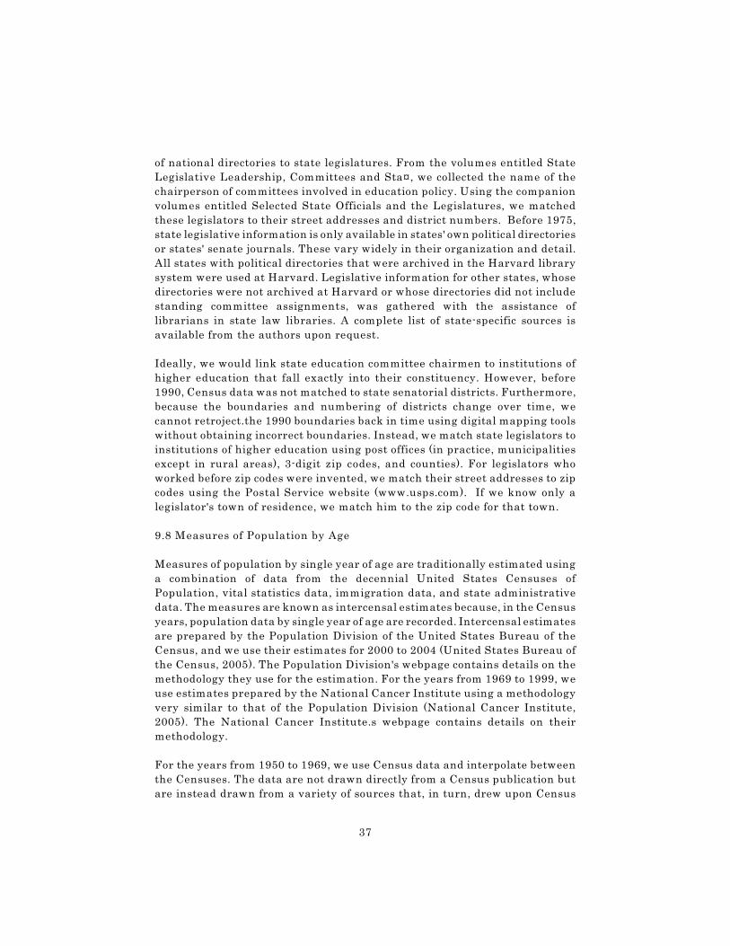
37

of national directories to state legislatures. From the volumes entitled State

Legislative Leadership, Committees and Sta¤, we collected the name of the

chairperson of committees involved in education policy. Using the companion

volumes entitled Selected State Officials and the Legislatures, we matched

these legislators to their street addresses and district numbers. Before 1975,

state legislative information is only available in states' own political directories

or states' senate journals. These vary widely in their organization and detail.

All states with political directories that were archived in the Harvard library

system were used at Harvard. Legislative information for other states, whose

directories were not archived at Harvard or whose directories did not include

standing committee assignments, was gathered with the assistance of

librarians in state law libraries. A complete list of state-specific sources is

available from the authors upon request.

Ideally, we would link state education committee chairmen to institutions of

higher education that fall exactly into their constituency. However, before

1990, Census data was not matched to state senatorial districts. Furthermore,

because the boundaries and numbering of districts change over time, we

cannot retroject.the 1990 boundaries back in time using digital mapping tools

without obtaining incorrect boundaries. Instead, we match state legislators to

institutions of higher education using post offices (in practice, municipalities

except in rural areas), 3-digit zip codes, and counties). For legislators who

worked before zip codes were invented, we match their street addresses to zip

codes using the Postal Service website (www.usps.com). If we know only a

legislator's town of residence, we match him to the zip code for that town.

9.8 Measures of Population by Age

Measures of population by single year of age are traditionally estimated using

a combination of data from the decennial United States Censuses of

Population, vital statistics data, immigration data, and state administrative

data. The measures are known as intercensal estimates because, in the Census

years, population data by single year of age are recorded. Intercensal estimates

are prepared by the Population Division of the United States Bureau of the

Census, and we use their estimates for 2000 to 2004 (United States Bureau of

the Census, 2005). The Population Division's webpage contains details on the

methodology they use for the estimation. For the years from 1969 to 1999, we

use estimates prepared by the National Cancer Institute using a methodology

very similar to that of the Population Division (National Cancer Institute,

2005). The National Cancer Institute.s webpage contains details on their

methodology.

For the years from 1950 to 1969, we use Census data and interpolate between

the Censuses. The data are not drawn directly from a Census publication but

are instead drawn from a variety of sources that, in turn, drew upon Census

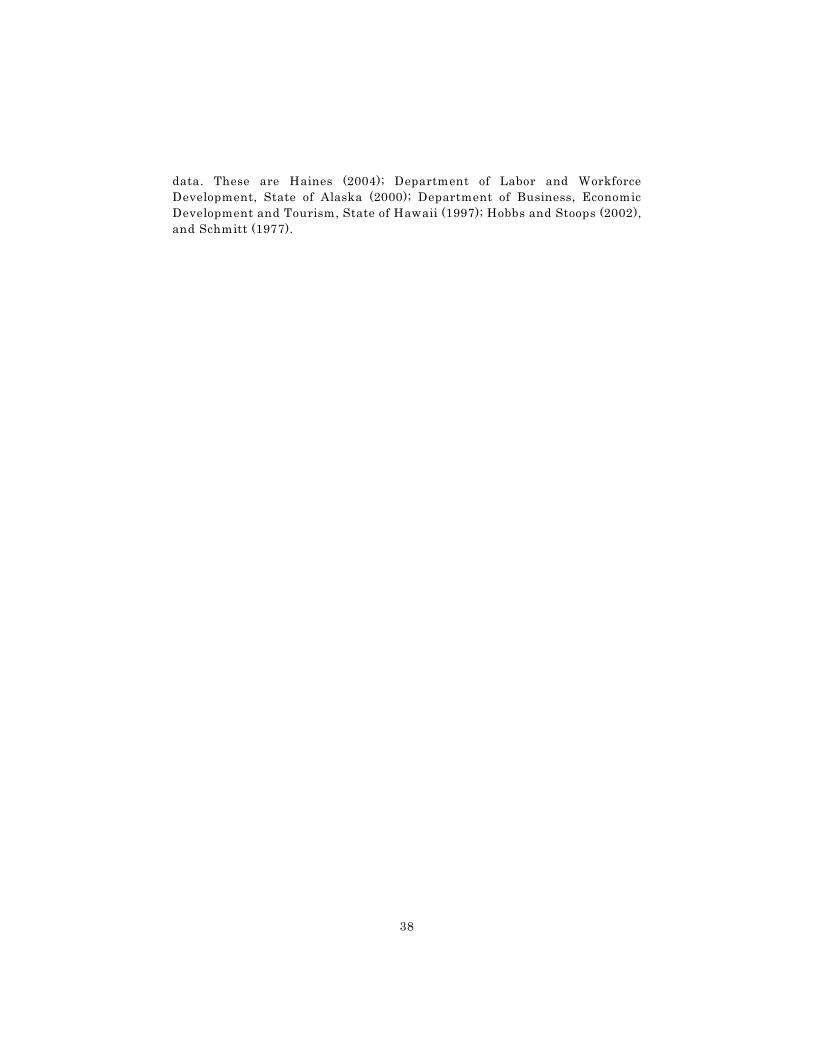
38

data. These are Haines (2004); Department of Labor and Workforce

Development, State of Alaska (2000); Department of Business, Economic

Development and Tourism, State of Hawaii (1997); Hobbs and Stoops (2002),

and Schmitt (1977).

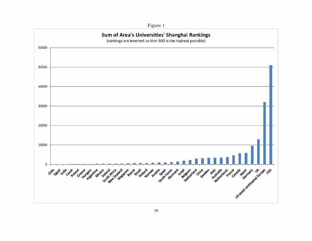
39

Figure 1

40

Figure 2

Figure 3

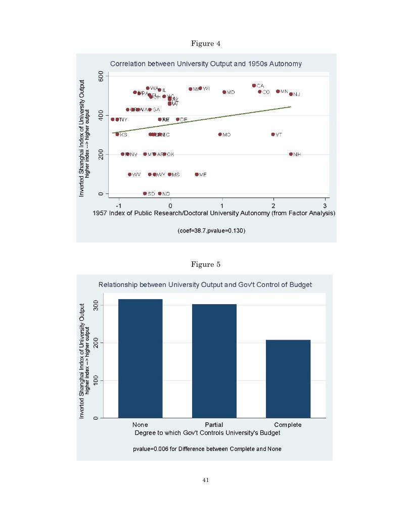
41

Figure 4

Figure 5

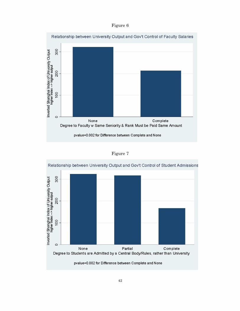
42

Figure 6

Figure 7

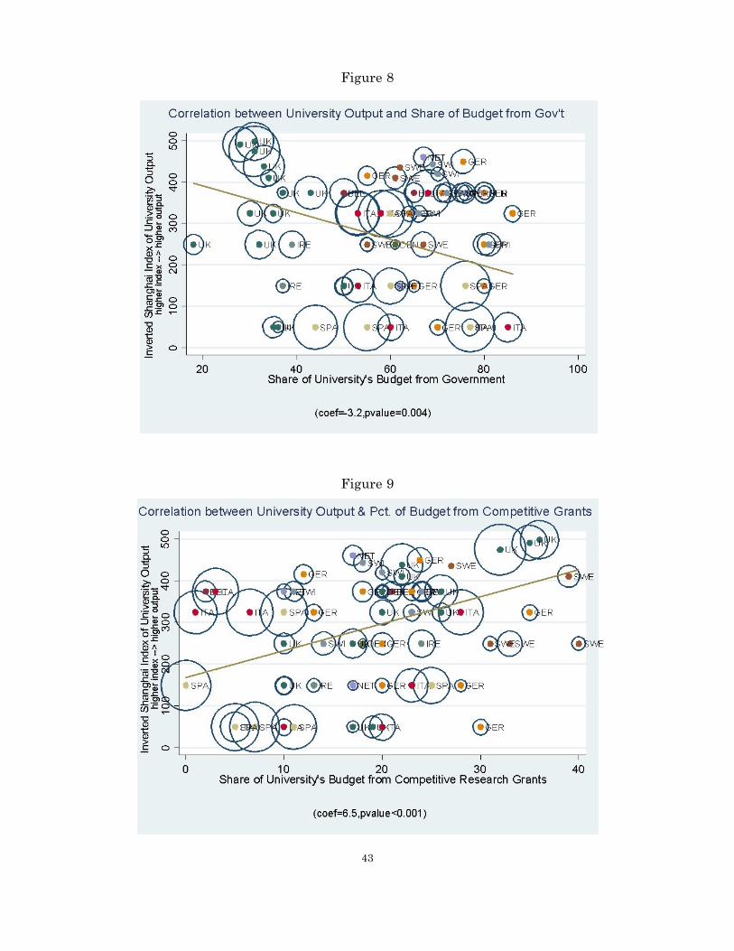
43

Figure 8

Figure 9

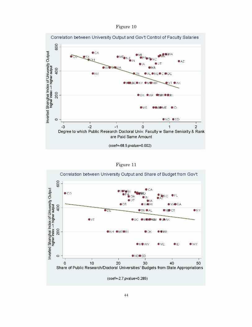
44

Figure 10

Figure 11

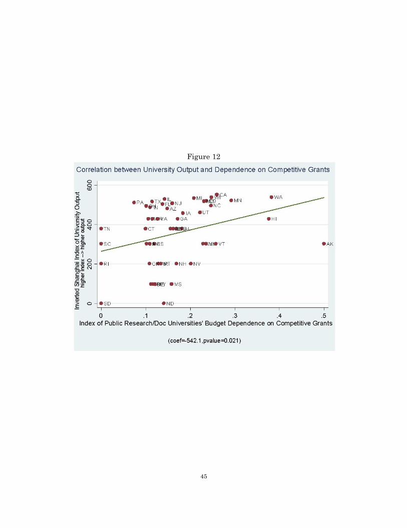
45

Figure 12

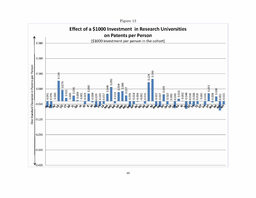
46

Figure 13

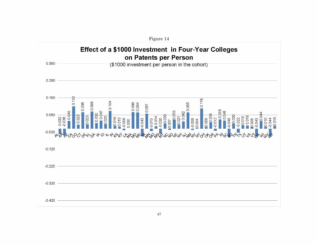
47

Figure 14

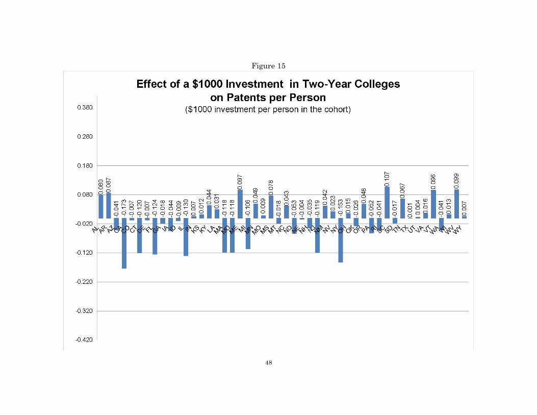
48

Figure 15

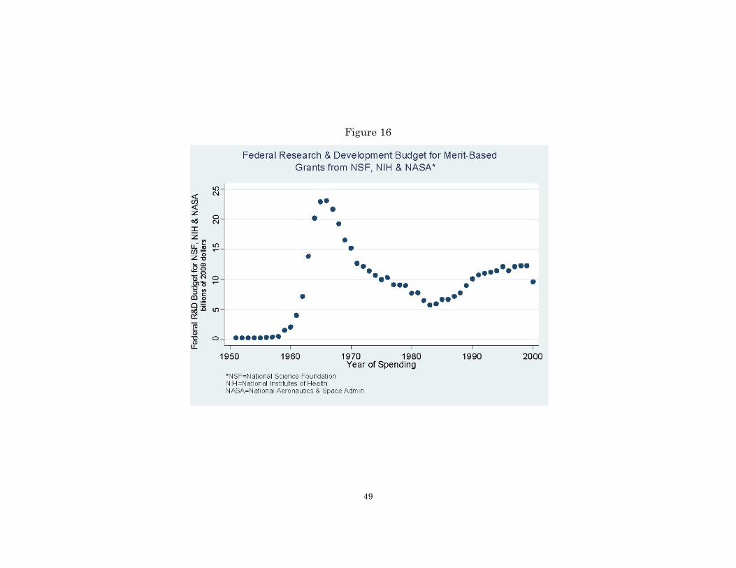
49

Figure 16

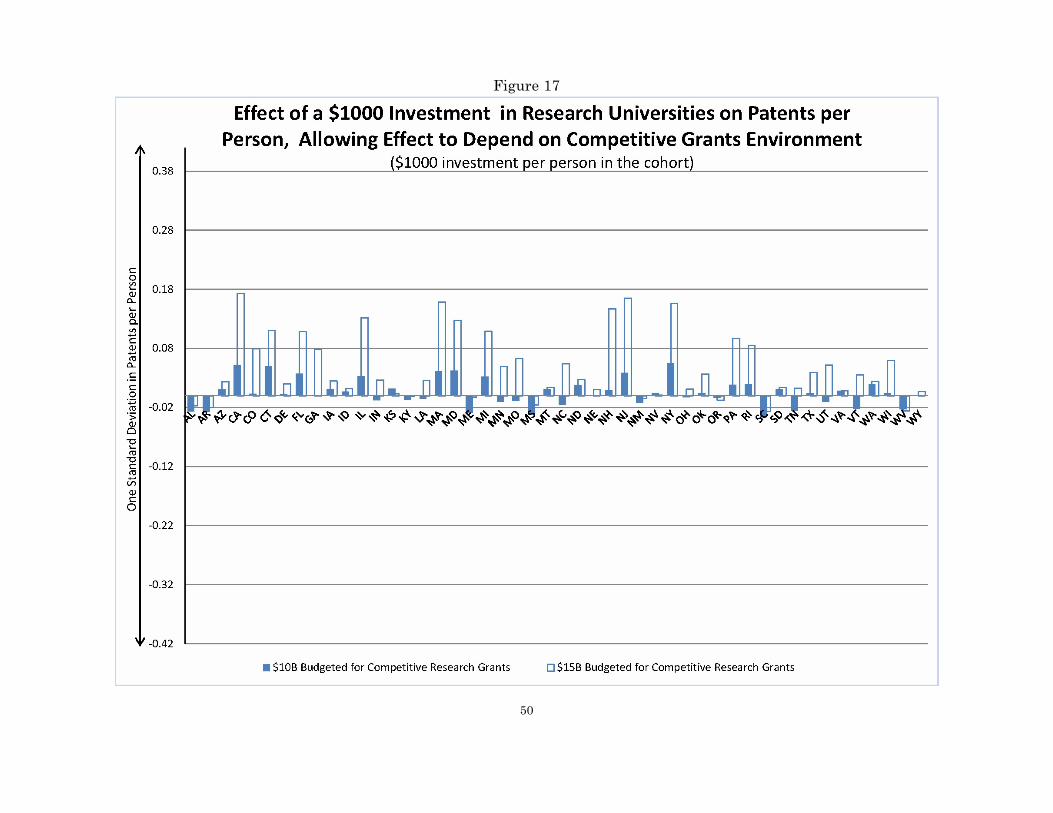
50

Figure 17

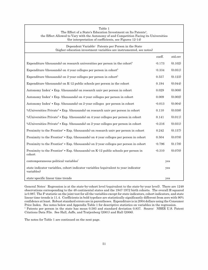
51

Table 1The Effect of a State's Education Investment on Its Patents ,a

the Effect Allowed to Vary with the Autonomy of and Competition Facing its Universities(for interpretation of coefficients, see Figures 12-14)

Dependent Variable: Patents per Person in the State(higher education investment variables are instrumented, see notes)

coeff. std.err

Expenditure (thousands) on research universities per person in the cohort -0.173 (0.102)b

Expenditure (thousands) on 4-year colleges per person in cohort -0.334 (0.051)b

Expenditure (thousands) on 2-year colleges per person in cohort 0.557 (0.123)b

Expenditure (thousands) on K-12 public schools per person in the cohort 0.194 (0.044)

Autonomy Index C Exp. (thousands) on research univ per person in cohort 0.029 (0.008)c

Autonomy Index C Exp. (thousands) on 4-year colleges per person in cohort 0.009 (0.002)c

Autonomy Index C Exp. (thousands) on 2-year colleges per person in cohort -0.013 (0.004)c

%Universities Private C Exp. (thousands) on research univ per person in cohort 0.110 (0.038)d

%Universities Private C Exp. (thousands) on 4-year colleges per person in cohort 0.141 (0.011)d

%Universities Private C Exp. (thousands) on 2-year colleges per person in cohort -0.216 (0.031)d

Proximity to the Frontier C Exp. (thousands) on research univ per person in cohort 0.242 (0.157)e

Proximity to the Frontier C Exp. (thousands) on 4-year colleges per person in cohort 0.504 (0.078)e

Proximity to the Frontier C Exp. (thousands) on 2-year colleges per person in cohort -0.796 (0.178)e

Proximity to the Frontier C Exp. (thousands) on K-12 public schools per person ine

cohort-0.310 (0.070)

contemporaneous political variables yesf

state indicator variables, cohort indicator variables (equivalent to year indicatorvariables)

yes

state-specific linear time trends yes

General Notes: Regression is at the state-by-cohort level (equivalent to the state-by-year level). There are 1248observations corresponding to the 48 continental states and the 1947-1972 birth cohorts. The overall R-squaredis 0.987. The F-statistic on the joint test for all the variables except for state indicators, cohort indicators, and statelinear time trends is 11.4. Coefficients in bold typeface are statistically significantly different from zero with 90%confidence at least. Robust standard errors are in parentheses. Expenditure is in 2004 dollars using the ConsumerPrice Index. See notes below and Appendix Table 1 for descriptive statistics on variables in the regression. Patents per person in the state has mean 0.583 and standard deviation 0.837. Source: NBER U.S. Patenta

Citations Data File. See Hall, Jaffe, and Tratjenberg (2001) and Hall (2006).

The notes for Table 1 are continued on the next page.

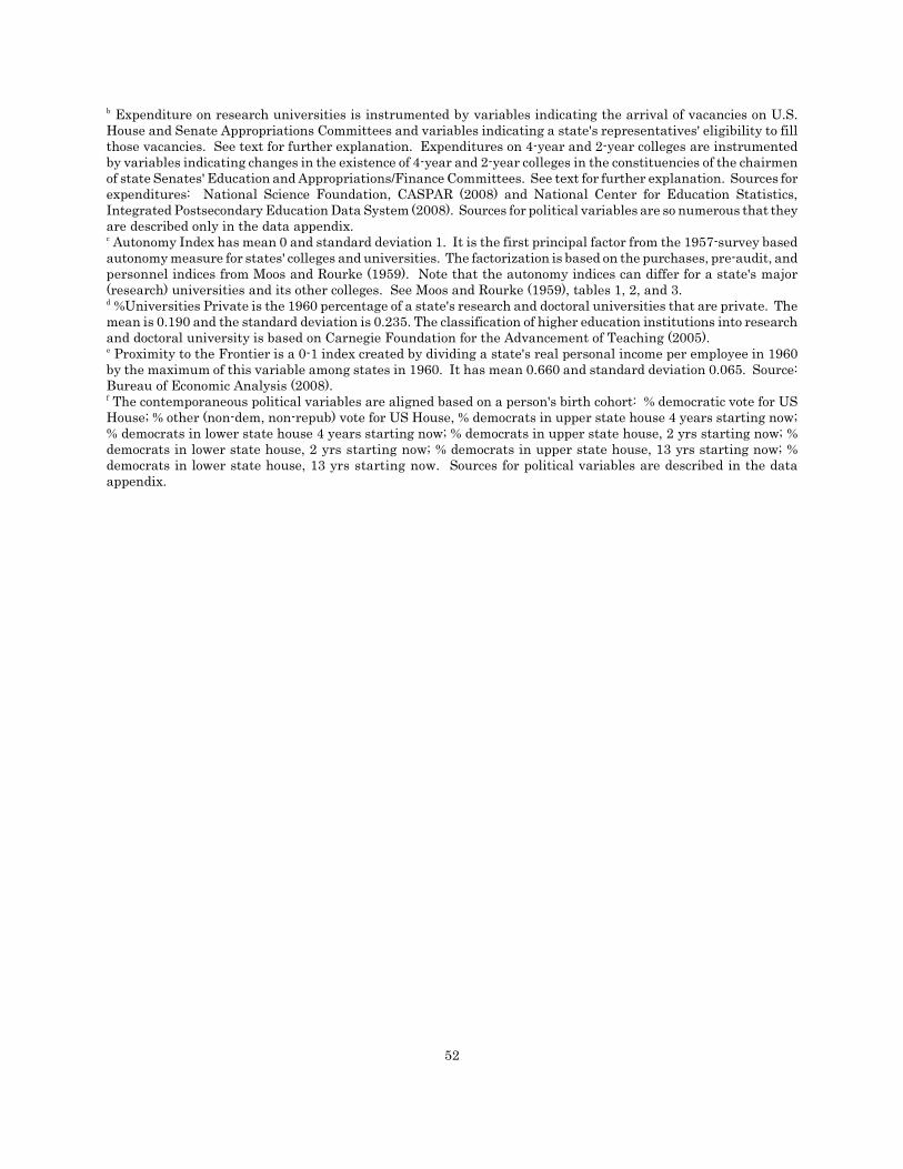
52

Expenditure on research universities is instrumented by variables indicating the arrival of vacancies on U.S.b

House and Senate Appropriations Committees and variables indicating a state's representatives' eligibility to fillthose vacancies. See text for further explanation. Expenditures on 4-year and 2-year colleges are instrumentedby variables indicating changes in the existence of 4-year and 2-year colleges in the constituencies of the chairmenof state Senates' Education and Appropriations/Finance Committees. See text for further explanation. Sources forexpenditures: National Science Foundation, CASPAR (2008) and National Center for Education Statistics,Integrated Postsecondary Education Data System (2008). Sources for political variables are so numerous that theyare described only in the data appendix. Autonomy Index has mean 0 and standard deviation 1. It is the first principal factor from the 1957-survey basedc

autonomy measure for states' colleges and universities. The factorization is based on the purchases, pre-audit, andpersonnel indices from Moos and Rourke (1959). Note that the autonomy indices can differ for a state's major(research) universities and its other colleges. See Moos and Rourke (1959), tables 1, 2, and 3. %Universities Private is the 1960 percentage of a state's research and doctoral universities that are private. Thed

mean is 0.190 and the standard deviation is 0.235. The classification of higher education institutions into researchand doctoral university is based on Carnegie Foundation for the Advancement of Teaching (2005). Proximity to the Frontier is a 0-1 index created by dividing a state's real personal income per employee in 1960e

by the maximum of this variable among states in 1960. It has mean 0.660 and standard deviation 0.065. Source:Bureau of Economic Analysis (2008). The contemporaneous political variables are aligned based on a person's birth cohort: % democratic vote for USf

House; % other (non-dem, non-repub) vote for US House, % democrats in upper state house 4 years starting now;% democrats in lower state house 4 years starting now; % democrats in upper state house, 2 yrs starting now; %democrats in lower state house, 2 yrs starting now; % democrats in upper state house, 13 yrs starting now; %democrats in lower state house, 13 yrs starting now. Sources for political variables are described in the dataappendix.

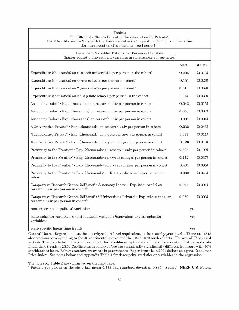
53

Table 2The Effect of a State's Education Investment on Its Patents ,a

the Effect Allowed to Vary with the Autonomy of and Competition Facing its Universities(for interpretation of coefficients, see Figure 16)

Dependent Variable: Patents per Person in the State(higher education investment variables are instrumented, see notes)

coeff. std.err.

Expenditure (thousands) on research universities per person in the cohort -0.208 (0.072)b

Expenditure (thousands) on 4-year colleges per person in cohort -0.151 (0.026)b

Expenditure (thousands) on 2-year colleges per person in cohort 0.348 (0.069)b

Expenditure (thousands) on K-12 public schools per person in the cohort 0.014 (0.030)

Autonomy Index C Exp. (thousands) on research univ per person in cohort -0.042 (0.015)c

Autonomy Index C Exp. (thousands) on research univ per person in cohort 0.006 (0.002)c

Autonomy Index C Exp. (thousands) on research univ per person in cohort -0.007 (0.004)c

%Universities Private C Exp. (thousands) on research univ per person in cohort -0.232 (0.046)d

%Universities Private C Exp. (thousands) on 4-year colleges per person in cohort 0.017 (0.011)d

%Universities Private C Exp. (thousands) on 2-year colleges per person in cohort -0.123 (0.018)d

Proximity to the Frontier C Exp. (thousands) on research univ per person in cohort 0.265 (0.109)e

Proximity to the Frontier C Exp. (thousands) on 4-year colleges per person in cohort 0.252 (0.037)e

Proximity to the Frontier C Exp. (thousands) on 2-year colleges per person in cohort -0.481 (0.095)e

Proximity to the Frontier C Exp. (thousands) on K-12 public schools per person ine

cohort-0.030 (0.045)

Competitive Research Grants (billions) C Autonomy Index C Exp. (thousands) onf c

research univ per person in cohortb

0.004 (0.001)

Competitive Research Grants (billions) C %Universities Private C Exp. (thousands) onf d

research univ per person in cohortb

0.029 (0.003)

contemporaneous political variables yesg

state indicator variables, cohort indicator variables (equivalent to year indicatorvariables)

yes

state-specific linear time trends yes

General Notes: Regression is at the state-by-cohort level (equivalent to the state-by-year level). There are 1248observations corresponding to the 48 continental states and the 1947-1972 birth cohorts. The overall R-squaredis 0.992. The F-statistic on the joint test for all the variables except for state indicators, cohort indicators, and statelinear time trends is 23.3. Coefficients in bold typeface are statistically significantly different from zero with 90%confidence at least. Robust standard errors are in parentheses. Expenditure is in 2004 dollars using the ConsumerPrice Index. See notes below and Appendix Table 1 for descriptive statistics on variables in the regression.

The notes for Table 2 are continued on the next page. Patents per person in the state has mean 0.583 and standard deviation 0.837. Source: NBER U.S. Patenta

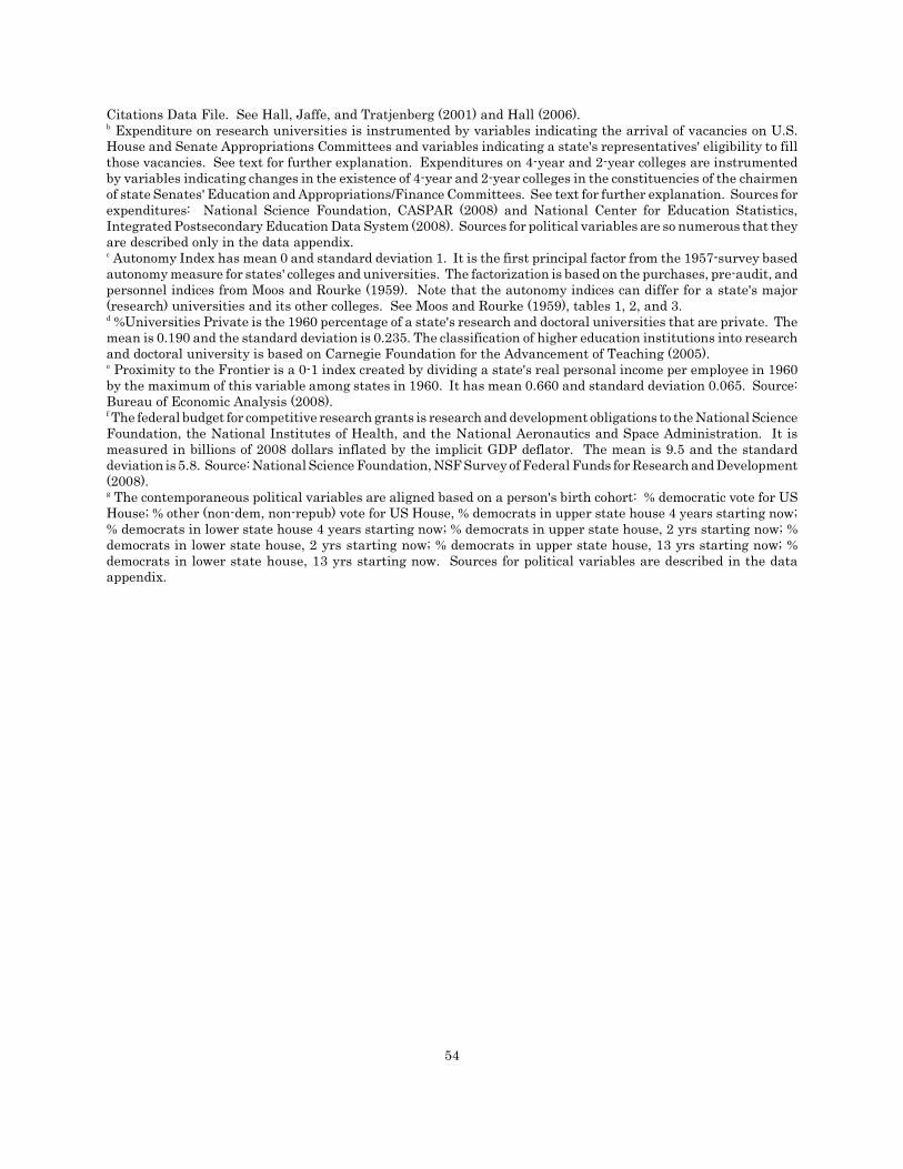
54

Citations Data File. See Hall, Jaffe, and Tratjenberg (2001) and Hall (2006). Expenditure on research universities is instrumented by variables indicating the arrival of vacancies on U.S.b

House and Senate Appropriations Committees and variables indicating a state's representatives' eligibility to fillthose vacancies. See text for further explanation. Expenditures on 4-year and 2-year colleges are instrumentedby variables indicating changes in the existence of 4-year and 2-year colleges in the constituencies of the chairmenof state Senates' Education and Appropriations/Finance Committees. See text for further explanation. Sources forexpenditures: National Science Foundation, CASPAR (2008) and National Center for Education Statistics,Integrated Postsecondary Education Data System (2008). Sources for political variables are so numerous that theyare described only in the data appendix. Autonomy Index has mean 0 and standard deviation 1. It is the first principal factor from the 1957-survey basedc

autonomy measure for states' colleges and universities. The factorization is based on the purchases, pre-audit, andpersonnel indices from Moos and Rourke (1959). Note that the autonomy indices can differ for a state's major(research) universities and its other colleges. See Moos and Rourke (1959), tables 1, 2, and 3. %Universities Private is the 1960 percentage of a state's research and doctoral universities that are private. Thed

mean is 0.190 and the standard deviation is 0.235. The classification of higher education institutions into researchand doctoral university is based on Carnegie Foundation for the Advancement of Teaching (2005). Proximity to the Frontier is a 0-1 index created by dividing a state's real personal income per employee in 1960e

by the maximum of this variable among states in 1960. It has mean 0.660 and standard deviation 0.065. Source:Bureau of Economic Analysis (2008). The federal budget for competitive research grants is research and development obligations to the National Sciencef

Foundation, the National Institutes of Health, and the National Aeronautics and Space Administration. It ismeasured in billions of 2008 dollars inflated by the implicit GDP deflator. The mean is 9.5 and the standarddeviation is 5.8. Source: National Science Foundation, NSF Survey of Federal Funds for Research and Development(2008). The contemporaneous political variables are aligned based on a person's birth cohort: % democratic vote for USg

House; % other (non-dem, non-repub) vote for US House, % democrats in upper state house 4 years starting now;% democrats in lower state house 4 years starting now; % democrats in upper state house, 2 yrs starting now; %democrats in lower state house, 2 yrs starting now; % democrats in upper state house, 13 yrs starting now; %democrats in lower state house, 13 yrs starting now. Sources for political variables are described in the dataappendix.

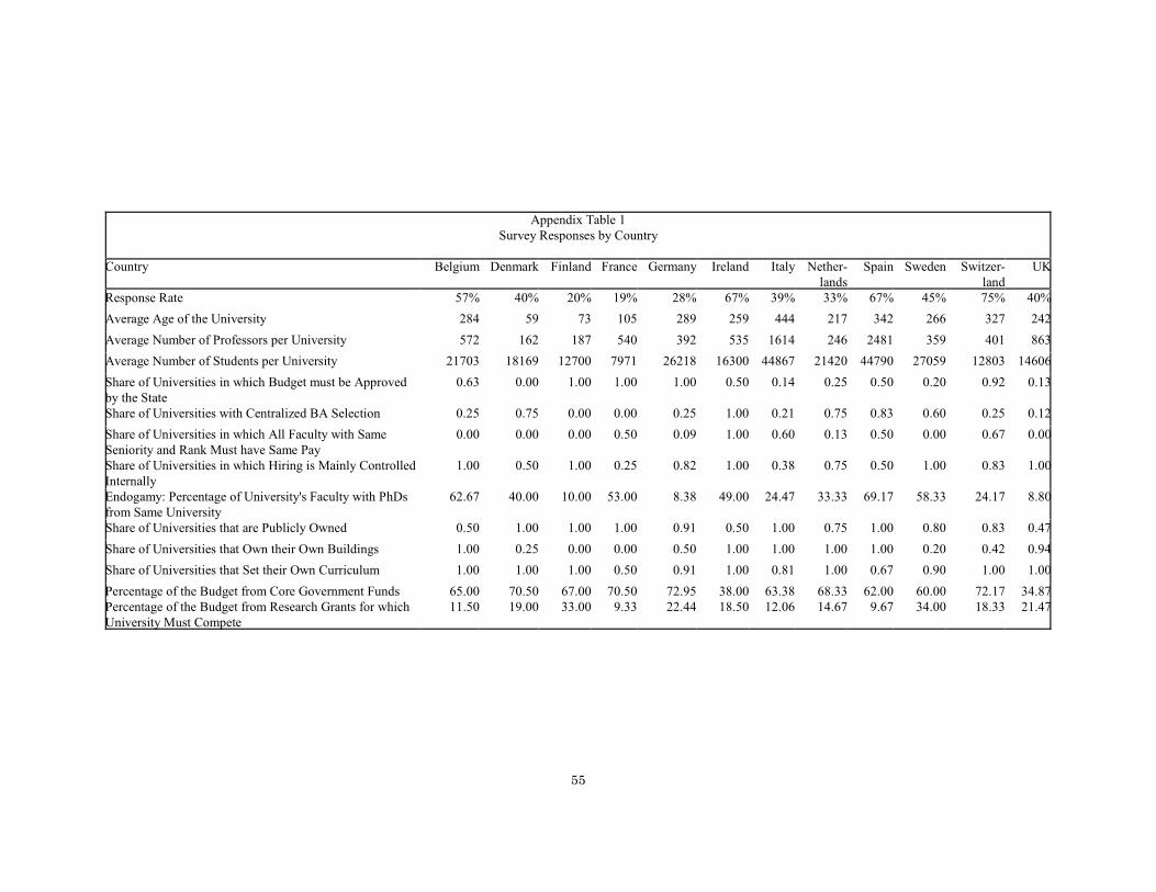
55

Appendix Table 1Survey Responses by Country

Country Belgium Denmark Finland France Germany Ireland Italy Nether-lands

Spain Sweden Switzer-land

UK

Response Rate 57% 40% 20% 19% 28% 67% 39% 33% 67% 45% 75% 40%

Average Age of the University 284 59 73 105 289 259 444 217 342 266 327 242

Average Number of Professors per University 572 162 187 540 392 535 1614 246 2481 359 401 863

Average Number of Students per University 21703 18169 12700 7971 26218 16300 44867 21420 44790 27059 12803 14606

Share of Universities in which Budget must be Approvedby the State

0.63 0.00 1.00 1.00 1.00 0.50 0.14 0.25 0.50 0.20 0.92 0.13

Share of Universities with Centralized BA Selection 0.25 0.75 0.00 0.00 0.25 1.00 0.21 0.75 0.83 0.60 0.25 0.12

Share of Universities in which All Faculty with SameSeniority and Rank Must have Same Pay

0.00 0.00 0.00 0.50 0.09 1.00 0.60 0.13 0.50 0.00 0.67 0.00

Share of Universities in which Hiring is Mainly ControlledInternally

1.00 0.50 1.00 0.25 0.82 1.00 0.38 0.75 0.50 1.00 0.83 1.00

Endogamy: Percentage of University's Faculty with PhDsfrom Same University

62.67 40.00 10.00 53.00 8.38 49.00 24.47 33.33 69.17 58.33 24.17 8.80

Share of Universities that are Publicly Owned 0.50 1.00 1.00 1.00 0.91 0.50 1.00 0.75 1.00 0.80 0.83 0.47

Share of Universities that Own their Own Buildings 1.00 0.25 0.00 0.00 0.50 1.00 1.00 1.00 1.00 0.20 0.42 0.94

Share of Universities that Set their Own Curriculum 1.00 1.00 1.00 0.50 0.91 1.00 0.81 1.00 0.67 0.90 1.00 1.00

Percentage of the Budget from Core Government Funds 65.00 70.50 67.00 70.50 72.95 38.00 63.38 68.33 62.00 60.00 72.17 34.87Percentage of the Budget from Research Grants for whichUniversity Must Compete

11.50 19.00 33.00 9.33 22.44 18.50 12.06 14.67 9.67 34.00 18.33 21.47

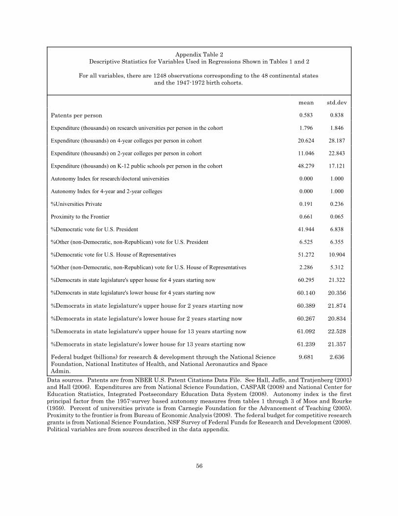
56

Appendix Table 2Descriptive Statistics for Variables Used in Regressions Shown in Tables 1 and 2

For all variables, there are 1248 observations corresponding to the 48 continental states and the 1947-1972 birth cohorts.

mean std.dev

Patents per person 0.583 0.838

Expenditure (thousands) on research universities per person in the cohort 1.796 1.846

Expenditure (thousands) on 4-year colleges per person in cohort 20.624 28.187

Expenditure (thousands) on 2-year colleges per person in cohort 11.046 22.843

Expenditure (thousands) on K-12 public schools per person in the cohort 48.279 17.121

Autonomy Index for research/doctoral universities 0.000 1.000

Autonomy Index for 4-year and 2-year colleges 0.000 1.000

%Universities Private 0.191 0.236

Proximity to the Frontier 0.661 0.065

%Democratic vote for U.S. President 41.944 6.838

%Other (non-Democratic, non-Republican) vote for U.S. President 6.525 6.355

%Democratic vote for U.S. House of Representatives 51.272 10.904

%Other (non-Democratic, non-Republican) vote for U.S. House of Representatives 2.286 5.312

%Democrats in state legislature's upper house for 4 years starting now 60.295 21.322

%Democrats in state legislature's lower house for 4 years starting now 60.140 20.356

%Democrats in state legislature's upper house for 2 years starting now 60.389 21.874

%Democrats in state legislature's lower house for 2 years starting now 60.267 20.834

%Democrats in state legislature's upper house for 13 years starting now 61.092 22.528

%Democrats in state legislature's lower house for 13 years starting now 61.239 21.357

Federal budget (billions) for research & development through the National ScienceFoundation, National Institutes of Health, and National Aeronautics and SpaceAdmin.

9.681 2.636

Data sources. Patents are from NBER U.S. Patent Citations Data File. See Hall, Jaffe, and Tratjenberg (2001)and Hall (2006). Expenditures are from National Science Foundation, CASPAR (2008) and National Center forEducation Statistics, Integrated Postsecondary Education Data System (2008). Autonomy index is the firstprincipal factor from the 1957-survey based autonomy measures from tables 1 through 3 of Moos and Rourke(1959). Percent of universities private is from Carnegie Foundation for the Advancement of Teaching (2005).Proximity to the frontier is from Bureau of Economic Analysis (2008). The federal budget for competitive researchgrants is from National Science Foundation, NSF Survey of Federal Funds for Research and Development (2008).Political variables are from sources described in the data appendix.