The Goods Market - Zentraler Informatikdiensthomepage.univie.ac.at/christina.zauner/Goods Market.pdf · Introduction to Macroeconomics (WS 2011) The Goods Market October 14th, 2011

The Goods Market

Introduction to Macroeconomics

WS 2011

October 14th, 2011

Introduction to Macroeconomics (WS 2011) The Goods Market October 14th , 2011 1 / 29

Recapitulation of the last lecture

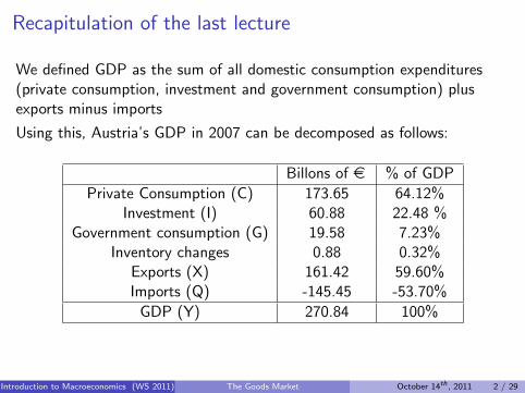
We defined GDP as the sum of all domestic consumption expenditures(private consumption, investment and government consumption) plusexports minus imports

Using this, Austria’s GDP in 2007 can be decomposed as follows:

Billons of e % of GDP

Private Consumption (C) 173.65 64.12%Investment (I) 60.88 22.48 %

Government consumption (G) 19.58 7.23%Inventory changes 0.88 0.32%

Exports (X) 161.42 59.60%Imports (Q) -145.45 -53.70%

GDP (Y) 270.84 100%


Recapitulation of the last lecture

IMPORTANT

A decomposition does however not explain how GDP will respond tosudden changes in one of its components.

In the following sessions we try to explain GDP.

In other words, we will try to understand the effect people’s consumptiondecision, firms’ investment decisions and government’s consumptiondecisions have on aggregate output using a simple model inspired by JohnMaynard Keynes.


The first step towards the IS-LM model

The IS-LM model was first presented informally by John MaynardKeynes in ”The General Theory of Employment, Interest, and Money”(published in 1936)

John Hicks presented the IS-LM model as we discuss it in 1936

The IS-LM model studies the simultaneous equilibrium on a goodsand a financial market

The IS-LM model is a static model, i.e. adjustments to theequilibrium occur instantaneously

The endogenous variables of the IS-LM model are output(production/income, Y) and the interest rate (endogenous variablesare determined in equilibrium (or explained by the model), whereasexogenous variables are taken as given)


The first step towards the IS-LM model

As a first step, we will discuss the equilibrium on an isolated goodsmarket where the level of real GDP will be determined by the equalityof supply (or production) and aggregate demand

After that, we will discuss the equilibrium on an isolated financialmarket where the interest rate will be determined by the equality ofmoney supply and money demand

Finally, we will connect the two markets by assuming that investmentdemand depends on the interest rate and by assuming that moneydemand depends on the level of real GDP.An equilibrium is then defined as a situation in which production anddemand are equal on the goods market and in which money demandequals money supply at the same time.


Assumptions of our Model

1 We are only concerned with the short run: prices are constant

2 There is only one good in the economy. This good is used for privateconsumption, for investment and for government consumption.

3 Firms are willing to supply any amount of the good at the given price⇒ in equilibrium supply will equal demand

4 The economy is closed, i.e. there are no exports or imports (and noother relationships with foreign countries such as people workingabroad, ...)


Discussion of Assumptions

Empirically, prices are indeed constant in the short run. This can beexplained by:

I menu costs: changing prices is associated with costs (”printing newmenus”) and will take some time

I Therefore, firms will not immediately respond to changes in demandwith changing the price they charge but instead simply change theirproduction (working overtime, ...)

Actually, people consume more than just one good. But we can thinkof the single good in the model as a whole consumer basket.Assumption 2 is only made for simplicity!

There are (almost) no closed economies. Assumption 4 is wrong, buta simplification! We will start discussing the model with an openeconomy at the end of the course.


Private Consumption (C)

Decompositions of GDP show that private consumption is by far themost important part of demand

Households base their demand decisions on their disposable incomeYD

We can define the consumption function of households as:

C = C (YD) with C ′ > 0

Disposable income of households is given by their income Y minusthe taxes they pay and plus the subsidies they receive, i.e. by

YD = Y − T

where T captures net taxes (taxes minus subsidies)


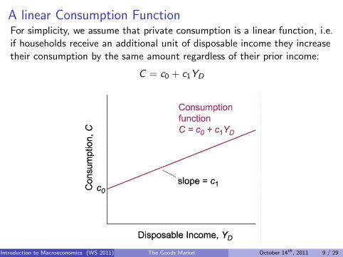
A linear Consumption FunctionFor simplicity, we assume that private consumption is a linear function, i.e.if households receive an additional unit of disposable income they increasetheir consumption by the same amount regardless of their prior income:

C = c0 + c1YD

55

© 2003 Prentice Hall Business Publishing© 2003 Prentice Hall Business Publishing Macroeconomics, 3/e Olivier BlanchardMacroeconomics, 3/e Olivier Blanchard Ch. 3 Ch. 3 –– Page Page 99

Consumption (Consumption (CC))

Consumption and Consumption and

Disposable IncomeDisposable Income

Consumption increases

with disposable income,

but less than one for

one.

C C YD

= ( )

Y Y TD

≡ −

C c c Y T= + −0 1

( )

© 2003 Prentice Hall Business Publishing© 2003 Prentice Hall Business Publishing Macroeconomics, 3/e Olivier BlanchardMacroeconomics, 3/e Olivier Blanchard Ch. 3 Ch. 3 –– Page Page 1010

Investment (Investment (II))

�� Variables that depend on other variables Variables that depend on other variables

within the model are called within the model are called endogenousendogenous. .

Variables that are not explained within the Variables that are not explained within the

model are called model are called exogenousexogenous. Investment . Investment

here is taken as given, or treated as an here is taken as given, or treated as an

exogenous variable:exogenous variable:

I I=


A linear Consumption Function

A linear consumption function can be fully described by two exogenouslygiven parameters:

the intercept c0I is referred to as autonomous consumption, i.e. consumption without

any disposable incomeI captures the level of consumption necessary for survival (so c0 > 0)I is financed by dissaving (selling assets or borrowing)

the slope c1I is referred to as the marginal propensity to consumeI captures by how much households increase their consumption if their

disposable income increases marginallyI 0 < c1 < 1


Investment (I)

For now, we will take investments as exogenously given, i.e. weassume that

I = I

for some fixed value I .

In order to establish the link with the financial market we will changethis assumption later on by assuming that investments dependnegatively on the interest rate and positively on production


Government Consumption (G)

Government consumption and taxes are exogenous parameters ofthe model, i.e. G = G for some fixed value G and T = T for somefixed value T

This assumption allows us to analyze question such as ”Whathappens when the government suddenly increases its consumption ortaxation?”

We will also be able to compare the effects of fiscal policy underdifferent regimes, e.g. with a government that wants to maintain abalanced budget or with a government that doesn’t care aboutrunning a budget deficit


Taxation

Assuming that the government only collects lump sum taxes (taxeswhich do not depend on households’ income, but are the same foreach income level) is again a simplification

Instead we can assume that government uses a linear tax scale, i.e.

T = t0 + t1Y

with 0 < t1 < 1


Equilibrium on the Goods Market

The goods market is in equilibrium if demand (Z ) and supply areequal

Using the definition of demand (Z ≡ C + I + G ) and the assumptionswe have made on C , I and G we get:

Z = c0 + c1(Y − T

)+ I + G

Supply in the economy is given by Y (recall that GDP can also bedefined as the value of the produced output in the economy)

The equilibrium condition for the goods market is therefore:

Y = Z

or equivalentlyY = c0 + c1

(Y − T

)+ I + G (1)


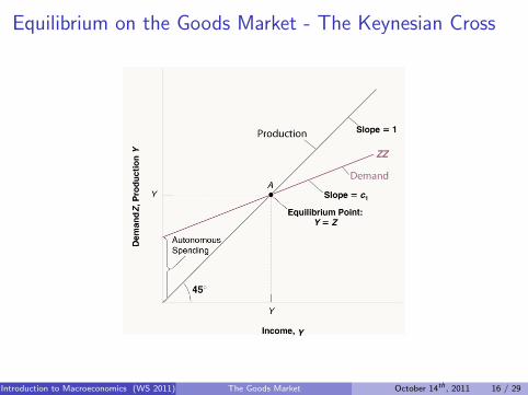
Equilibrium on the Goods Market - Graphical Solution

In order to find the equilibrium level for Y we can use a graphical analysis:

1 we plot demand Z as a function of income ⇒ the line ZZ in thediagram

2 we plot supply/production Y as a function of income ⇒ 45◦ line(Y = Y )

3 we look for the intersection of the two lines (setting demand equal tosupply)


Equilibrium on the Goods Market - The Keynesian Cross

Cha

pter

3:

The

Goo

ds M

arke

t

Copyright © 2009 Pearson Education, Inc. Publishing as Prentice Hall • Macroeconomics, 5/e • Olivier Blanchard 18 of 32

3-3 The Determination of Equilibrium Output

0 1 1( )Z c I G cT cY

First, plot production as a function of income.

Second, plot demand as a function of income.

In Equilibrium, production equals demand.

Equilibrium output is determined by the condition that production be equal to demand.

Equilibrium in the Goods Market

Figure 3 - 2

Using a Graph


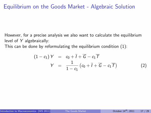
Equilibrium on the Goods Market - Algebraic Solution

However, for a precise analysis we also want to calculate the equilibriumlevel of Y algebraically:This can be done by reformulating the equilibrium condition (1):

(1− c1)Y = c0 + I + G − c1T

Y =1

1− c1

(c0 + I + G − c1T

)(2)


Equilibrium on the Goods Market - Interpretation of theSolution

From (2) we see that equilibrium output Y is a multiple of autonomousspending c0 + I + G − c1T :

Goods market equilibrium output is positive provided thatautonomous spending is positive. This case is very likely since it onlyrequires that the surplus of the government T − G is not too large.

If autonomous spending were negative, there would be no equilibriumoutput level (for all positive Y there would be excess supply on thegoods market) ⇒ we rule this case out by assuming that autonomousspending is positive

The factor 11−c1 is referred to as the multiplier and is larger than 1

⇒ if autonomous spending (e.g. G ) is increased by e 1, the value ofequilibrium output will increase by more than e 1


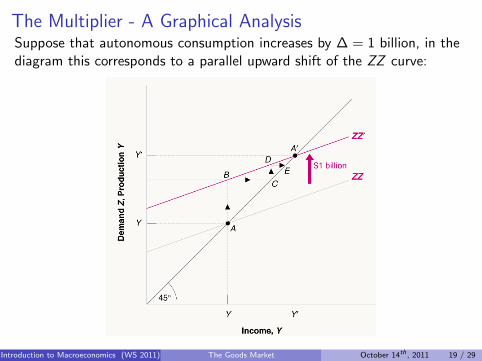
The Multiplier - A Graphical AnalysisSuppose that autonomous consumption increases by ∆ = 1 billion, in thediagram this corresponds to a parallel upward shift of the ZZ curve:

Cha

pter

3:

The

Goo

ds M

arke

t

Copyright © 2009 Pearson Education, Inc. Publishing as Prentice Hall • Macroeconomics, 5/e • Olivier Blanchard 19 of 32

Using a Graph

An increase in autonomous spending has a more than one- for-one effect on equilibrium output.

The Effects of an Increase in Autonomous Spending on Output

Figure 3 - 3

3-3 The Determination of Equilibrium Output


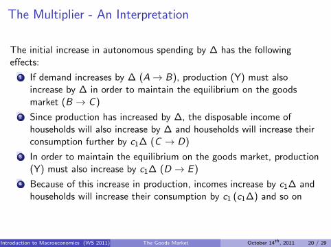
The Multiplier - An Interpretation

The initial increase in autonomous spending by ∆ has the followingeffects:

1 If demand increases by ∆ (A→ B), production (Y) must alsoincrease by ∆ in order to maintain the equilibrium on the goodsmarket (B → C )

2 Since production has increased by ∆, the disposable income ofhouseholds will also increase by ∆ and households will increase theirconsumption further by c1∆ (C → D)

3 In order to maintain the equilibrium on the goods market, production(Y) must also increase by c1∆ (D → E )

4 Because of this increase in production, incomes increase by c1∆ andhouseholds will increase their consumption by c1 (c1∆) and so on


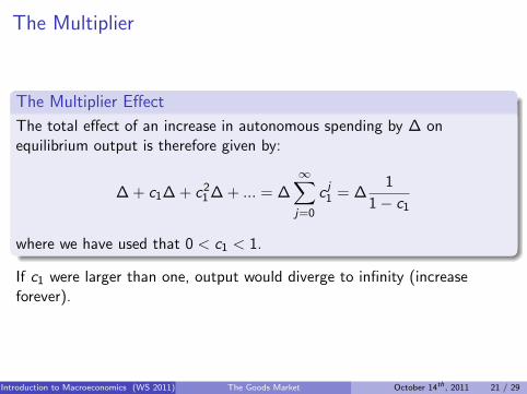
The Multiplier

The Multiplier Effect

The total effect of an increase in autonomous spending by ∆ onequilibrium output is therefore given by:

∆ + c1∆ + c21∆ + ... = ∆∞∑j=0

c j1 = ∆1

1− c1

where we have used that 0 < c1 < 1.

If c1 were larger than one, output would diverge to infinity (increaseforever).


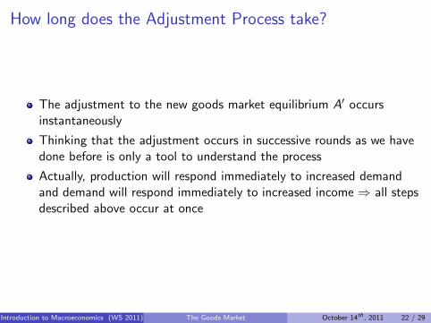
How long does the Adjustment Process take?

The adjustment to the new goods market equilibrium A′ occursinstantaneously

Thinking that the adjustment occurs in successive rounds as we havedone before is only a tool to understand the process

Actually, production will respond immediately to increased demandand demand will respond immediately to increased income ⇒ all stepsdescribed above occur at once


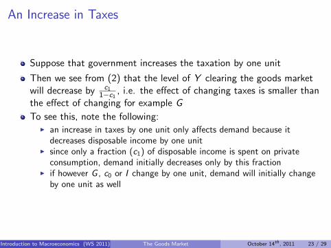
An Increase in Taxes

Suppose that government increases the taxation by one unit

Then we see from (2) that the level of Y clearing the goods marketwill decrease by c1

1−c1 , i.e. the effect of changing taxes is smaller thanthe effect of changing for example G

To see this, note the following:I an increase in taxes by one unit only affects demand because it

decreases disposable income by one unitI since only a fraction (c1) of disposable income is spent on private

consumption, demand initially decreases only by this fractionI if however G , c0 or I change by one unit, demand will initially change

by one unit as well


A Different Way of Defining Goods Market Equilibrium

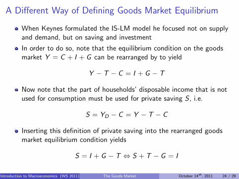
When Keynes formulated the IS-LM model he focused not on supplyand demand, but on saving and investment

In order to do so, note that the equilibrium condition on the goodsmarket Y = C + I + G can be rearranged by to yield

Y − T − C = I + G − T

Now note that the part of households’ disposable income that is notused for consumption must be used for private saving S , i.e.

S = YD − C = Y − T − C

Inserting this definition of private saving into the rearranged goodsmarket equilibrium condition yields

S = I + G − T ⇔ S + T − G = I



Since S captures private saving and T − G constitutes public saving,this equilibrium condition says that in a goods market equilibrium Yis such that investment equals total saving in the economy

This is also why the goods market equilibrium will be represented bythe IS-curve in the full model



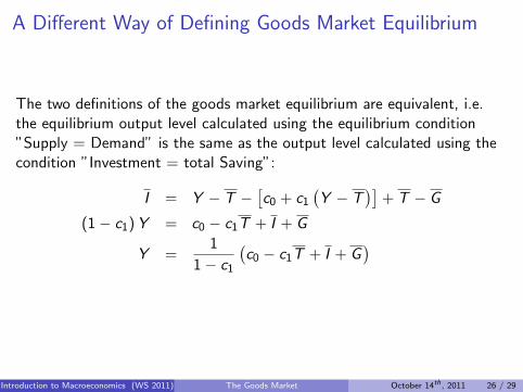
The two definitions of the goods market equilibrium are equivalent, i.e.the equilibrium output level calculated using the equilibrium condition”Supply = Demand” is the same as the output level calculated using thecondition ”Investment = total Saving”:

I = Y − T −[c0 + c1

(Y − T

)]+ T − G

(1− c1)Y = c0 − c1T + I + G

Y =1

1− c1

(c0 − c1T + I + G

)


The Paradox of Saving/Thrift

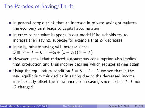
In general people think that an increase in private saving stimulatesthe economy as it leads to capital accumulation

In order to see what happens in our model if households try toincrease their saving, suppose for example that c0 decreases

Initially, private saving will increase sinceS ≡ Y − T − C = −c0 + (1− c1) (Y − T )

However, recall that reduced autonomous consumption also impliesthat production and thus income declines which reduces saving again

Using the equilibrium condition I = S + T − G we see that in thenew equilibrium this decline in saving due to the decreased incomemust exactly offset the initial increase in saving since neither I , T norG changed


The Paradox of Saving/Thrift

Conclusion

In the short run, an attempt to increase private saving only results indecreased output or income but leaves private saving in the newequilibrium at its initial level.


Remarks

Demand and supply on the goods market are real variables (we areconcerned with quantities!).

Hence, we must assume that e.g. the consumption decision (i.e. howmany goods to buy) also depends on real income (i.e. how manygoods can be bought with the given nominal income) ⇒ the variableY refers to real GDP rather than to nominal GDP


Documents

The Goods Market - Zentraler Informatikdiensthomepage.univie.ac.at/christina.zauner/Goods Market.pdf · Introduction to Macroeconomics (WS 2011) The Goods Market October 14th, 2011