The Gibbs Centroid Sampler

W232–W237 Nucleic Acids Research, 2007, Vol. 35, Web Server issuedoi:10.1093/nar/gkm265

The Gibbs Centroid SamplerWilliam A. Thompson1,*, Lee A. Newberg2,3, Sean Conlan4, Lee Ann McCue5 and

Charles E. Lawrence1

1Center for Computational Molecular Biology and the Division of Applied Mathematics, Brown University,Providence, RI 02912, USA, 2The Wadsworth Center, New York State Department of Health, Albany,NY 12201, USA, 3Department of Computer Science, Rensselaer Polytechnic Institute, Troy, NY 12180,USA, 4Columbia University, New York, NY 10032, USA and 5Pacific Northwest National Laboratory,Richland, WA 99352, USA

Received January 31, 2007; Revised March 27, 2007; Accepted April 8, 2007

ABSTRACT

The Gibbs Centroid Sampler is a software packagedesigned for locating conserved elements in bio-polymer sequences. The Gibbs Centroid Samplerreports a centroid alignment, i.e. an alignment thathas the minimum total distance to the set ofsamples chosen from the a posteriori probabilitydistribution of transcription factor binding-sitealignments. In so doing, it garners informationfrom the full ensemble of solutions, rather thanonly the single most probable point that is the targetof many motif-finding algorithms, including itspredecessor, the Gibbs Recursive Sampler.Centroid estimators have been shown to yieldsubstantial improvements, in both sensitivity andpositive predictive values, to the prediction of RNAsecondary structure and motif finding. TheGibbs Centroid Sampler, along with interactivetutorials, an online user manual, and informationon downloading the software, is available at: http://bayesweb.wadsworth.org/gibbs/gibbs.html.

INTRODUCTION

The identification of transcription factor binding sites(TFBSs) in the promoters of genes is a critical step in thedelineation of the genetic regulatory network of anorganism. A number of motif discovery algorithms havebeen developed over the past decade and a half, for thedetection of cis-regulatory sites (1). Most of thesealgorithms depend, in one way or another, on finding anoptimal alignment of motif sites. In this article, wedescribe the web server for an improved motif discoveryalgorithm, the Gibbs Centroid Sampler, which finds acentroid alignment. The centroid alignment is the align-ment that has the minimum total distance to the set ofsamples chosen from the a posteriori probability

distribution of TFBS alignments. By focusing on theregion of solution space containing the most posteriorprobability, rather than on the single solution that is mostprobable, this approach significantly enhances the pre-dictive power of the algorithm. In computational experi-ments using simulated proteobacterial and yeast data (2),the centroid sampler showed improved specificity andpositive predictive value over algorithms that report anoptimal solution.

The Gibbs Centroid Sampler is an improved version ofthe Gibbs Recursive Sampler (3), which has been usedextensively in the identification of TFBSs (4–8), and hasbeen available at our Web site for some time (3,9). Thesoftware currently available at the Web site retains all ofthe features of the previous versions, including searchesfor multiple motif types, multiple instances (sites) of amotif, palindromic motifs, motifs of varying widths and aheterogeneous background frequency model (see (3) fordescriptions of these and other features). The users’choices of options are entered through a web form,described below, and the output is returned to the user viae-mail. In addition to the new algorithmic features, theWeb site has been updated to include extensive tutorialson the use of the Gibbs sampling software for prokaryoticphylogenetic footprinting and for the analysis of prokary-otic co-expression data.

The Gibbs Centroid Sampler

A key feature of most sequence-based Gibbs sampling andexpectation maximization algorithms (10,11), is the use ofa probabilistic score that is maximized. Typically, thealignment that has the maximum of this score is reportedto the user. Previous versions of the Gibbs Sampler usedthe posterior probability of the alignment, called the MAP(maximum a posteriori probability) (12), as a measure ofthe quality of the alignment, and thus the alignment thatproduced the highest posterior probability (i.e. the MAPalignment) was returned. The reported MAP was calcu-lated as the logarithm of the alignment probability minus

*To whom correspondence should be addressed. Tel: þ1-401-863-2048; Email: [email protected]

� 2007 The Author(s)

This is an Open Access article distributed under the terms of the Creative Commons Attribution Non-Commercial License (http://creativecommons.org/licenses/

by-nc/2.0/uk/) which permits unrestricted non-commercial use, distribution, and reproduction in any medium, provided the original work is properly cited.

Downloaded from https://academic.oup.com/nar/article-abstract/35/suppl_2/W232/2920797by gueston 11 February 2018

the logarithm of an empty or background alignment.Thus, the reported value was a measure of the extent towhich a particular alignment was better than background.

The use of methods such as this, which seek to obtainglobal or local optimal solutions to inference problems, iscommon in computational biology. Typically, however,the probability of even the best arrangement of motif sitesis extremely small. That is, since motif detection is a high-dimensional problem, from a Bayesian viewpoint, the datalikelihood will contain an immense number of terms, ofwhich the optimal solution is simply one. From thisperspective, the question arises, ‘How representative is theoptimum when its probability is very small compared tothe overall probability mass?’

It has been shown in RNA secondary structureprediction (13) and TFBS discovery algorithms (2,14)that reliance on the optimal solution can be misleadingand can adversely affect prediction accuracy. Specifically,Ding et al. (13,15) showed that centroid estimates reducederrors in RNA secondary structure prediction by 30%,while simultaneously improving sensitivity, and Newberget al. (2) showed similar substantial improvements overalgorithms finding local optima for TFBS discovery insequences from phylogenetically closely related species.Centroid solutions garner information from the fullensemble of solutions, while MAP solutions focusexclusively on the single most probable point.

The centroid sampling algorithm

The user supplies to the algorithm a collection ofsequences in FASTA format and enters several para-meters, such as motif widths, as described below. Thecentroid algorithm begins in a manner similar to previousGibbs sampling algorithms. It is initialized with a,typically random, alignment. From this alignment, motifmodels are calculated (12). The sampling procedure thenproceeds through the following steps:

(i) A sequence is selected, and the probability of eachpossible number of sites, up to the maximumspecified by the user, is calculated based on thecurrent model;

(ii) the number of sites is sampled;(iii) the predicted positions and types of the sites are

sampled based on their probabilities, calculated asdescribed by Thompson et al. (3);

(iv) the motif models are updated based on the sampledsites in all sequences.

An iteration of the algorithm consists of the completionof Steps 1–4 for each sequence. In previous versions, thisprocess repeated until the MAP failed to increase for afixed number of iterations. To obtain a sampling solution,we allow the algorithm to repeat the above procedurethrough a burn-in period, typically 2000 iterations. Theburn-in period is required for the sampler to move awayfrom transient effects of the particular initial conditions.After the burn-in period, the sampler proceeds, againthrough a fixed number of iterations (typically 8000).During this sampling process, the algorithm trackseach sampled position. The entire process (burn-in and

sampling iterations) is repeated with a number of differentrandom starting alignments called ‘seeds’. By default,20 seeds are used. The samples from each seed areaccumulated, and a centroid alignment solution isobtained from the accumulated samples; the centroid isthe alignment that minimizes the sum of the pair-wisedistances between it and each of the alignments in thecollection. Thus, the centroid is defined in terms of adistance measure between pairs of proposed alignments.The centroid alignment is calculated via a dynamicprogramming algorithm.In previous versions of the sampler, the model update

step (Step 4 above) was accomplished using the predictiveupdate method (12). The centroid sampler performs themodel update step by sampling a new model from theposterior Dirichlet distribution of motif or backgroundmodels. Starting with the existing model �, the algorithmdraws a new model, �p, using the motif or backgroundcounts from Dir (cþ b), where Dir is the Dirichletdistribution, and c and b are the current count andpseudo-count vectors. While predictive update workswhen at most one new binding site is chosen betweenmotif model updates, it is not entirely appropriate in thepresent context, where multiple binding sites are chosenbetween model updates. This new model update method isof greatest value in the identification of sites amongaligned sequences derived from multiple phylogeneticallyrelated species (2).

The Gibbs SamplerWeb Site

The Gibbs Sampler Web site consists of three layers, eachoffering an increasing number of options for control of thesampling process. The first page, shown in Figure 1, allowsthe user to input sequences, select the version of the GibbsSampler, and control the basic motif parameters (16).

Figure 1. The basic Gibbs Centroid Sampler entry screen.

Nucleic Acids Research, 2007, Vol. 35,Web Server issue W233


While we continue to make earlier versions available forselection on this page, in most circumstances the centroidsampler should return better results (2). An e-mailaddress, a set of sequences in FASTA format, an optionalinitial guess of the total number of sites, the number ofconserved positions in the motif sites, and the maximumallowable number of sites in any one sequence are enteredon this page. The estimate of the number of sites affectsthe initial starting solution for the burn-in process. If itis not supplied, the default of one site for each motiftype for each sequence is used. We have found this defaultadequate for most datasets, and the centroid sampler isrelatively insensitive to reasonably small changes in thisvalue. The number of conserved positions in the motifmodel(s) is a required parameter. This value sets theminimum width of the predicted sites, although sites mayfragment to a greater width by the inclusion of non-conserved positions (12). Motif widths for multiple modelscan be entered, although it is best to use no more motifmodels than is reasonable given the number of expectedTFBS types. Increasing the number of motif modelsbeyond the number of relevant site types should notadversely affect the solutions, if the number of burn-in andsample iterations is adequate (described below), becauseextra models will not sample sites sufficiently to beincluded in the centroid. However, as the number ofmodels increases, the program runtime increases(described below). The maximum number of sites in asingle sequence is also a required parameter for thecentroid sampler. The value entered for this parametershould be based on knowledge of the biological systemunder study. For example, when analyzing bacterialintergenic sequences for TFBSs, a value of two or threeis typically used, whereas for eukaryotic data, this numberis typically set higher. This parameter sets the maximumfor the total sum of all motif sites in any one sequence.The sequence data can be pasted into the entry window oruploaded from a file. Each entry field has an associatedhyperlink, which leads to a page describing the requireddata format. From this entry screen, default options willbe automatically selected for the sampling parameters.The defaults for the centroid sampler include the use ofa heterogeneous background model (16), 20 random seeds,a burn-in period of 2000 iterations and a sampling periodof 8000 iterations.

Control of sampling parameters

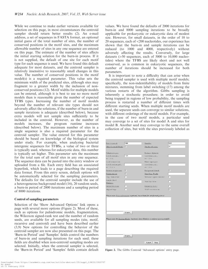
Selection of the ‘Show Advanced Options’ link opens apage with several more options (Figure 2). Most of these,such as options for palindromic models, fragmentation,the Wilcoxon signed-rank test and the number of randomseeds, are available for all sampling modes (site, motif,recursive and centroid) and have been described earlier(3,9) New options for controlling the behavior of thecentroid sampler are now also presented on this page. The‘Burn-in Period’ and ‘Samples’ fields control the numbersof burn-in and sampling iterations for each seed; thesefields are disabled when non-centroid sampling modes areselected. Initially, when the centroid sampler is selected,the ‘Burn-in Period’ and ‘Samples’ fields contain default

values. We have found the defaults of 2000 iterations forburn-in and 8000 sampling iterations to be broadlyapplicable for prokaryotic or eukaryotic data of modestsize. However, for small datasets, in the order of 10 to20 sequences, each of5200 nucleotides, our experience hasshown that the burn-in and sample iterations can bereduced (to 1000 and 4000, respectively) withoutadversely affecting the results. Conversely, for largedatasets (450 sequences, each of 5000 to 10,000 nucleo-tides) where the TFBS are likely short and not wellconserved, as is common in eukaryotic sequences, thenumber of iterations should be increased for bothparameters.

It is important to note a difficulty that can arise whenthe centroid sampler is used with multiple motif models;specifically, the non-indentifiability of models from finitemixtures, stemming from label switching (17) among thevarious restarts of the algorithm. Gibbs sampling isinherently a stochastic procedure; in order to avoidbeing trapped in regions of low probability, the samplingprocess is restarted a number of different times withdifferent starting seeds. When multiple motif models areused, the separate seeds can converge to similar solutions,with different orderings of the motif models. For example,in the case of two motif models, a particular seedmay converge to a set of sites for model A and sites formodel B. Another seed may converge to the same overallcollection of sites, but with the sites previously labeled as

Figure 2. The Gibbs Centroid ‘Advanced options’ entry page.

W234 Nucleic Acids Research, 2007, Vol. 35,Web Server issue


model A now labeled as model B, and sites previouslylabeled as model B now labeled as model A. The centroidsolution is obtained by summing the number of times agiven position (i.e. site) is sampled across all restarts andmodels, which means that sites from multiple models arenot separated in the output. Furthermore, differentfragmentation models (12) can be generated among thedifferent seed runs, giving rise to a collection of centroidsites that differ in length, and making it difficult tovisualize the TFBSs in a more traditional probabilitymatrix representation.

To address these two difficulties, the selection of the‘Align Centroid Model’ option causes the Gibbs CentroidSampler to use the Gibbs Recursive Sampler to align thecollection of centroid sites. In the case of multiple models,this process will separate the sites into related groups, andthus aid identification of the different site types. Thisprocess can also give the user insight into which positionsin the models are highly conserved. It is important to notethat the resulting alignment is neither a MAP alignmentnor a centroid alignment of the complete set of datasequences. It is provided only to lend additional insightinto the centroid solution.

Program output

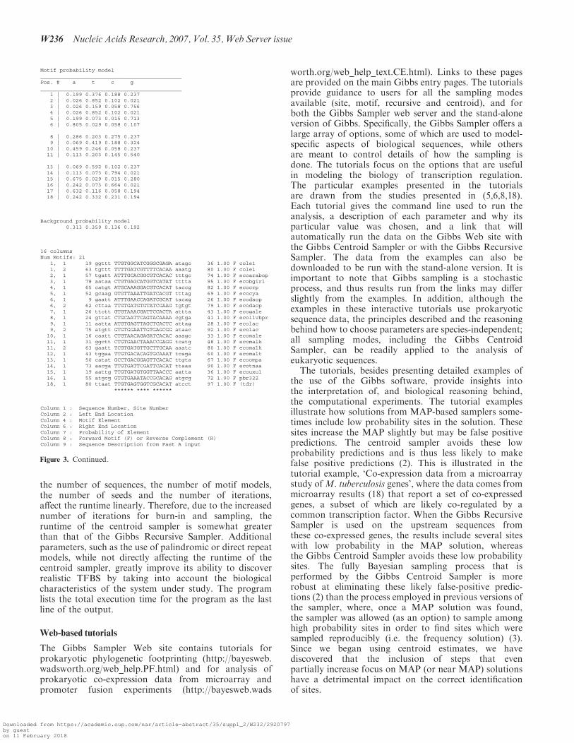
Program output is returned via e-mail. The initial portionof the Gibbs Centroid Sampler output is identical to thatof the other versions of the sampler, simply providing alist of the options used for the current run, followed by alist of the FASTA headings for the input sequences (see (3)for an example). Following these is the list of the sitesmaking up the centroid model. Figure 3 shows the resultsfor a set of 18 Escherichia coli sequences; these sequencesare well studied, known to contain binding sites for thecyclic AMP receptor protein (Crp) (11), and are provided asa test dataset when the Gibbs Sampler software is down-loaded. The results in Figure 3 were generated using thecentroid sampler with a motif width of 16, a palindromicmotif model requirement, a maximum number of sites persequence of two, heterogeneous background composition,the default number of restarts (20 seeds), the default burn-in(2000 iterations) and the default centroid sampling periods(8000 iterations). The motif models were allowed tofragment to a width of 24 bases.

At the top of Figure 3 is the set of sites making up thecentroid; the centroid sites are listed in upper case, andflanking positions are in lower case. The sites correspondwell with the DNaseI footprinted sites for these sequences(11). The variation in the length of the sites is a result ofdifferent fragmentation models generated during thesampling periods (mentioned above). The dynamic pro-gram that calculates the centroid can be found elsewhere[see the supplementary material for (2)]. The legend belowthe list of sites identifies the various columns of theoutput. The probability column shows the samplingfrequencies for these sites. These sampling frequenciesare an estimate of the probabilities that the cognatetranscription factors bind at the predicted sites.

The second part of Figure 3 shows an alignment of thecentroid sites. The program generates this alignment by

taking the collection of sites in the centroid, plus theirflanking sequences, and using the Gibbs RecursiveSampler to find the best alignment among this set ofsites, with at most one site in each sequence. As such, thisis neither a centroid nor an optimal alignment. It isprovided simply to allow the user to identify different sitetypes (when multiple motif models were used) and tovisualize which positions are highly conserved in thecentroid sites. The format of this alignment is identical tothat of the Gibbs Recursive Sampler previously describedin (3).

Performance

The underlying algorithm for the Gibbs Centroid Samplerand the Gibbs Recursive Sampler is a forward–backwardalgorithm (7). The forward step is the most computeintensive part of the algorithm, with runtime increasing asthe square of the length of the individual sequences; thus,the most important factor affecting runtime is the lengthof the individual sequences. Other parameters, such as

====================================================================== ========================== CENTROID RESULTS ========================== ======================================================================

1, 1 11 tttgt GCTGGTTTTTGTGGCATCGGGCG agaat 33 0.64 cole1 1, 2 54 gtgaa AGACTGTTTTTTTGATCGTTTTC acaaa 76 0.98 cole1 2, 1 56 ttgat TATTTGCACGGCGTCACAC tttgc 74 0.98 ecoarabop 3, 1 78 aataa CTGTGAGCATGGTCATATTTTTA tcaat 100 0.89 ecobgirl 4, 1 55 tgatg TACTGCATGTATGCAAAGGACGT cacat 77 0.82 ecocrp 5, 1 48 atcag CAAGGTGTTAAATTGATCACGTT ttaga 70 0.72 ecocya 6, 1 5 agtg AATTATTTGAACCAGATCGCATTA cagtg 28 0.97 ecodaop 6, 2 67 ttgtg ATGTGTATCGAAGTGTGTTGCGG agtag 89 0.83 ecodaop 7, 1 31 gtgta AACGATTCCACTAATTTATTCCA tgtca 53 0.89 ecogale 8, 1 29 ctgca ATTCAGTACAAAACGTGATCAAC ccctc 51 0.89 ecoilvbpr 9, 1 8 cgcaa TTAATGTGAGTTAGCTCACTC attag 28 0.97 ecolac 9, 2 73 gtatg TTGTGTGGAATTGTGAGCGGATA acaat 95 0.66 ecolac 10, 1 11 accgc CAATTCTGTAACAGAGATCAC acaaa 31 0.97 ecomale 11, 1 31 ggctt CTGTGAACTAAACCGAGGTCATG taagg 53 0.50 ecomalk 11, 2 56 atgta AGGAATTTCGTGATGTTGCTT gcaaa 76 0.78 ecomalk 12, 1 41 tttgg AATTGTGACACAGTGCAAATTCA gacac 63 0.93 ecomalt 13, 1 48 ttcat ATGCCTGACGGAGTTCACACTTG taagt 70 0.79 ecoompa 14, 1 78 ttgtg ATTCGATTCACATTTAAACAA tttca 98 0.89 ecotnaa 15, 1 15 gtgaa ATTGTTGTGATGTGGTTAACCCA attag 37 0.53 ecouxu1 16, 1 53 atatg CGGTGTGAAATACCGCACAGATG cgtaa 75 0.83 pbr322 18, 1 75 gaaag TTAATTTGTGAGTGGTCGCACAT atcct 97 0.99 (tdr) Num Sites: 21

Column 1 : Sequence Number, Site Number Column 2 : Left End Location Column 4 : Motif Element Column 6 : Right End Location Column 7 : Probability of Element Column 8 : Sequence Description from FastA input

====================================================================== ======================== Aligned Centroid Sites ====================== ======================================================================

------------------------------------------------------------------------- MOTIF a

Motif model (residue frequency x 100)____________________________________________ Pos. # a t c g Info _____________________________ 1 | 19 38 19 23 0.0 2 | . 90 9 . 1.0 3 | . 14 4 80 1.0 4 | . 90 9 . 1.0 5 | 19 4 . 76 0.9 6 | 85 . 4 9 0.9

8 | 28 19 28 23 0.1 9 | 4 42 19 33 0.2 10 | 47 23 4 23 0.1 11 | 9 19 14 57 0.4

13 | 4 61 9 23 0.3 14 | 9 4 85 . 1.4 15 | 71 . . 28 0.8 16 | 23 4 71 . 1.1 17 | 66 9 4 19 0.4 18 | 23 33 23 19 0.0

nonsite 28 32 16 22 site 25 28 19 26

Figure 3. Output from the Gibbs Centroid Sampler.



the number of sequences, the number of motif models,the number of seeds and the number of iterations,affect the runtime linearly. Therefore, due to the increasednumber of iterations for burn-in and sampling, theruntime of the centroid sampler is somewhat greaterthan that of the Gibbs Recursive Sampler. Additionalparameters, such as the use of palindromic or direct repeatmodels, while not directly affecting the runtime of thecentroid sampler, greatly improve its ability to discoverrealistic TFBS by taking into account the biologicalcharacteristics of the system under study. The programlists the total execution time for the program as the lastline of the output.

Web-based tutorials

The Gibbs Sampler Web site contains tutorials forprokaryotic phylogenetic footprinting (http://bayesweb.wadsworth.org/web_help.PF.html) and for analysis ofprokaryotic co-expression data from microarray andpromoter fusion experiments (http://bayesweb.wads

worth.org/web_help_text.CE.html). Links to these pagesare provided on the main Gibbs entry pages. The tutorialsprovide guidance to users for all the sampling modesavailable (site, motif, recursive and centroid), and forboth the Gibbs Sampler web server and the stand-aloneversion of Gibbs. Specifically, the Gibbs Sampler offers alarge array of options, some of which are used to model-specific aspects of biological sequences, while othersare meant to control details of how the sampling isdone. The tutorials focus on the options that are usefulin modeling the biology of transcription regulation.The particular examples presented in the tutorialsare drawn from the studies presented in (5,6,8,18).Each tutorial gives the command line used to run theanalysis, a description of each parameter and why itsparticular value was chosen, and a link that willautomatically run the data on the Gibbs Web site withthe Gibbs Centroid Sampler or with the Gibbs RecursiveSampler. The data from the examples can also bedownloaded to be run with the stand-alone version. It isimportant to note that Gibbs sampling is a stochasticprocess, and thus results run from the links may differslightly from the examples. In addition, although theexamples in these interactive tutorials use prokaryoticsequence data, the principles described and the reasoningbehind how to choose parameters are species-independent;all sampling modes, including the Gibbs CentroidSampler, can be readily applied to the analysis ofeukaryotic sequences.

The tutorials, besides presenting detailed examples ofthe use of the Gibbs software, provide insights intothe interpretation of, and biological reasoning behind,the computational experiments. The tutorial examplesillustrate how solutions from MAP-based samplers some-times include low probability sites in the solution. Thesesites increase the MAP slightly but may be false positivepredictions. The centroid sampler avoids these lowprobability predictions and is thus less likely to makefalse positive predictions (2). This is illustrated in thetutorial example, ‘Co-expression data from a microarraystudy ofM. tuberculosis genes’, where the data comes frommicroarray results (18) that report a set of co-expressedgenes, a subset of which are likely co-regulated by acommon transcription factor. When the Gibbs RecursiveSampler is used on the upstream sequences fromthese co-expressed genes, the results include several siteswith low probability in the MAP solution, whereasthe Gibbs Centroid Sampler avoids these low probabilitysites. The fully Bayesian sampling process that isperformed by the Gibbs Centroid Sampler is morerobust at eliminating these likely false-positive predic-tions (2) than the process employed in previous versions ofthe sampler, where, once a MAP solution was found,the sampler was allowed (as an option) to sample amonghigh probability sites in order to find sites which weresampled reproducibly (i.e. the frequency solution) (3).Since we began using centroid estimates, we havediscovered that the inclusion of steps that evenpartially increase focus on MAP (or near MAP) solutionshave a detrimental impact on the correct identificationof sites.

Motif probability model ____________________________________________ Pos. # a t c g ____________________________________________ 1 | 0.199 0.376 0.188 0.237 2 | 0.026 0.852 0.102 0.021 3 | 0.026 0.159 0.058 0.756 4 | 0.026 0.852 0.102 0.021 5 | 0.199 0.073 0.015 0.713 6 | 0.805 0.029 0.058 0.107

8 | 0.286 0.203 0.275 0.237 9 | 0.069 0.419 0.188 0.324 10 | 0.459 0.246 0.058 0.237 11 | 0.113 0.203 0.145 0.540

13 | 0.069 0.592 0.102 0.237 14 | 0.113 0.073 0.794 0.021 15 | 0.675 0.029 0.015 0.280 16 | 0.242 0.073 0.664 0.021 17 | 0.632 0.116 0.058 0.194 18 | 0.242 0.332 0.231 0.194

Background probability model 0.313 0.359 0.136 0.192

16 columns Num Motifs: 21 1, 1 19 ggttt TTGTGGCATCGGGCGAGA atagc 36 1.00 F cole1 1, 2 63 tgttt TTTTGATCGTTTTCACAA aaatg 80 1.00 F cole1 2, 1 57 tgatt ATTTGCACGGCGTCACAC tttgc 74 1.00 F ecoarabop 3, 1 78 aataa CTGTGAGCATGGTCATAT tttta 95 1.00 F ecobgirl 4, 1 65 catgt ATGCAAAGGACGTCACAT taccg 82 1.00 F ecocrp 5, 1 52 gcaag GTGTTAAATTGATCACGT tttag 69 1.00 F ecocya 6, 1 9 gaatt ATTTGAACCAGATCGCAT tacag 26 1.00 F ecodaop 6, 2 62 cttaa TTGTGATGTGTATCGAAG tgtgt 79 1.00 F ecodaop 7, 1 26 ttctt GTGTAAACGATTCCACTA attta 43 1.00 F ecogale 8, 1 24 gttat CTGCAATTCAGTACAAAA cgtga 41 1.00 F ecoilvbpr 9, 1 11 aatta ATGTGAGTTAGCTCACTC attag 28 1.00 F ecolac 9, 2 75 atgtt GTGTGGAATTGTGAGCGG ataac 92 1.00 F ecolac 10, 1 16 caatt CTGTAACAGAGATCACAC aaagc 33 1.00 F ecomale 11, 1 31 ggctt CTGTGAACTAAACCGAGG tcatg 48 1.00 F ecomalk 11, 2 63 gaatt TCGTGATGTTGCTTGCAA aaatc 80 1.00 F ecomalk 12, 1 43 tggaa TTGTGACACAGTGCAAAT tcaga 60 1.00 F ecomalt 13, 1 50 catat GCCTGACGGAGTTCACAC ttgta 67 1.00 F ecoompa 14, 1 73 aacga TTGTGATTCGATTCACAT ttaaa 90 1.00 F ecotnaa 15, 1 19 aattg TTGTGATGTGGTTAACCC aatta 36 1.00 F ecouxu1 16, 1 55 atgcg GTGTGAAATACCGCACAG atgcg 72 1.00 F pbr322 18, 1 80 ttaat TTGTGAGTGGTCGCACAT atcct 97 1.00 F (tdr) ****** **** ******

Column 1 : Sequence Number, Site Number Column 2 : Left End Location Column 4 : Motif Element Column 6 : Right End Location Column 7 : Probability of Element Column 8 : Forward Motif (F) or Reverse Complement (R) Column 9 : Sequence Description from Fast A input

Figure 3. Continued.

W236 Nucleic Acids Research, 2007, Vol. 35,Web Server issue


Additional features

The Gibbs Centroid Sampler can be used for the analysisof amino-acid sequences. The link from the main GibbsWeb site page leads to a page allowing the entry of amino-acid sequences. The Web site also contains a link to anonline user guide, which describes the various parametersand their input formats, has detailed descriptions of theoutput and lists possible error messages and their causes.The Gibbs Sampler Web site allows a maximum of1000 sequences of no longer than 10,000 nucleotides inlength. Users with larger datasets are directed to use thestand-alone version of the Gibbs Sampler.

ACKNOWLEDGEMENTS

The research is supported by the United StatesDepartment of Energy grant DE-FG02-04ER63942 toC.E.L. and L.A.M., and the United States NationalInstitutes of Health grants R01-HG01257 to CEL,2P20-RR01-5578-06 to Walter Atwood, and K25-HG003291 to L.A.N. The assistance of the WadsworthCenter Bioinformatics Core Facility and the BrownUniversity Center for Computational Molecular Biologyis greatly appreciated. PNNL is operated by Battelle forthe US Department of Energy under Contract DE-AC06-76RLO 1830. Funding to pay the Open Access publicationcharges for this article was provided by Department ofEnergy grant DE-FG02-04ER63942.

Conflict of interest statement. None declared.

REFERENCES

1. Sandve,G. and Drablos,F. (2006) A survey of motif discoverymethods in an integrated framework. Biology Direct., 1, 11.

2. Newberg,L., Thompson,W.A., Conlan,S.P., Smith,T.M.,McCue,L.A. and Lawrence,C.E. (2007) A phylogenetic Gibbssampler that yields centroid solutions for cis regulatory siteprediction. Bioinformatics, Accepted.

3. Thompson,W., Rouchka,E.C. and Lawrence,C.E. (2003) GibbsRecursive Sampler: finding transcription factor binding sites.Nucleic Acids Res., 31, 3580–3585.

4. Conlan,S., Lawrence,C. and McCue,L.A. (2005)Rhodopseudomonas palustris Regulons Detected by Cross-Species

Analysis of Alphaproteobacterial Genomes. Appl. Environ.Microbiol., 71, 7442–7452.

5. McCue,L., Thompson,W., Carmack,C., Ryan,M.P., Liu,J.S.,Derbyshire,V. and Lawrence,C.E. (2001) Phylogenetic footprintingof transcription factor binding sites in proteobacterial genomes.Nucleic Acids Res., 29, 774–782.

6. McCue,L.A., Thompson,W., Carmack,C.S. and Lawrence,C.E.(2002) Factors influencing the identification of transcription factorbinding sites by cross-species comparison. Genome Res., 12,1523–1532.

7. Thompson,W., Palumbo,M.J., Wasserman,W.W., Liu,J.S. andLawrence,C.E. (2004) Decoding Human Regulatory Circuits.Genome Res., 14, 1967–1974.

8. Florczyk,M.A., McCue,L.A., Purkayastha,A., Currenti,E.,Wolin,M.J. and McDonough,K.A. (2003) A Family ofacr-Coregulated Mycobacterium tuberculosis Genes Shares aCommon DNA Motif and Requires Rv3133c (dosR or devR) forExpression. Infect. Immun., 71, 5332–5343.

9. Thompson,W., McCue,L.A. and Lawrence,C.E. (2005)In Baxevanis,A.D., Davison,D.B., Page,R.D.M., Petsko,G.A.,Stein,L.D. and Stormo,G.D. (eds), Current Protocols inBioinformatics, John Wiley & Sons, Inc., New York, NY,pp. 2.8.1–2.8.38.

10. Bailey,T.L. and Elkan,C. (1995) Unsupervised Learningof Multiple Motifs in Biopolymers using EM. Mach Learn,21, 51–80.

11. Lawrence,C.E. and Reilly,A.A. (1990) An expectationmaximization (EM) algorithm for the identification and character-ization of common sites in unaligned biopolymer sequences.Proteins: Struct. Funct. Genet., 7, 41–51.

12. Liu,J., Neuwald,A. and Lawrence,C. (1995) Bayesian models formultiple local sequence alignment and Gibbs sampling strategies.JASA, 90, 432, 1156–1170.

13. Ding,Y.E., Chan,C.Y. and Lawrence,C.E. (2005) RNA secondarystructure prediction by centroids in a Boltzmann weightedensemble. RNA, 11, 1157–1166.

14. Thompson,W., Conlan,S., McCue,L.A. and Lawrence,C.E. (2007)In Bergman,N. (ed.), Methods in Molecular Biology, ComparativeGenomics, Humana Press, 1, 403–423.

15. Ding,Y., Chan,C.Y. and Lawrence,C.E. (2006) Clustering ofRNA Secondary Structures with Application to Messenger RNAs.J Mol. Biol., 359, 554.

16. Liu,J. and Lawrence,C. (1999) Bayesian inference on biopolymermodels. Bioinformatics, 15, 38–52.

17. Stephens,M. (2000) Dealing with label switching in mixturemodels. J. R. Stat. Soc.: Series B (Statistical Methodology),62, 795–809.

18. Sherman,D.R., Voskuil,M., Schnappinger,D., Liao,R., Harrell,M.I.and Schoolnik,G.K. (2001) Regulation of the Mycobacteriumtuberculosis hypoxic response gene encoding alpha -crystallin.PNAS, 98, 7534–7539.



Documents

The Gibbs Centroid Sampler