Embed Size (px)
Citation preview
Axel Gandy and Luitgard A. M Veraart
A Bayesian methodology for systemic risk assessment in financial networks Article (Accepted version) (Refereed)
Original citation: Gandy, Axel and Veraart, Luitgard A. M. (2016) A Bayesian methodology for systemic risk assessment in financial networks. Management Science . ISSN 0025-1909 © 2016 INFORMS This version available at: http://eprints.lse.ac.uk/66312/ Available in LSE Research Online: May 2016 LSE has developed LSE Research Online so that users may access research output of the School. Copyright © and Moral Rights for the papers on this site are retained by the individual authors and/or other copyright owners. Users may download and/or print one copy of any article(s) in LSE Research Online to facilitate their private study or for non-commercial research. You may not engage in further distribution of the material or use it for any profit-making activities or any commercial gain. You may freely distribute the URL (http://eprints.lse.ac.uk) of the LSE Research Online website. This document is the author’s final accepted version of the journal article. There may be differences between this version and the published version. You are advised to consult the publisher’s version if you wish to cite from it.
A Bayesian methodology for systemic risk assessment in financial
networks
Axel Gandy ∗
Imperial College London
Luitgard A. M. Veraart †
London School of Economics and Political Science
May 3, 2016
Abstract
We develop a Bayesian methodology for systemic risk assessment in financial networks such as the
interbank market. Nodes represent participants in the network and weighted directed edges represent
liabilities. Often, for every participant, only the total liabilities and total assets within this network are
observable. However, systemic risk assessment needs the individual liabilities. We propose a model
for the individual liabilities, which, following a Bayesian approach, we then condition on the observed
total liabilities and assets and, potentially, on certain observed individual liabilities. We construct a
Gibbs sampler to generate samples from this conditional distribution. These samples can be used in
stress testing, giving probabilities for the outcomes of interest. As one application we derive default
probabilities of individual banks and discuss their sensitivity with respect to prior information included
to model the network. An R-package implementing the methodology is provided.
Key words: Financial network, unknown interbank liabilities, systemic risk, Bayes, MCMC, Gibbs
sampler, power law.
1 IntroductionAssessing systemic risk in financial systems is a key concern for regulators and policy makers. We think
of systemic risk as the risk that some external or economic shock causes a participant in the financial system
to default on their obligations which then leads to severe knock-on effects to other participants, such as their
default; see (Hurd, 2015, Section 1.2) for a discussion of different definitions of systemic risk.
Participants in these financial systems consist of various types of institutions, e.g. banks, hedge funds,
pension funds or insurance companies. As banks are key players for systemic risk assessment we will, for
simplicity, refer to all participants in the financial system as banks.∗Imperial College London, Department of Mathematics, South Kensington Campus, London, SW7 2AZ, UK,
[email protected]†London School of Economics and Political Science, Department of Mathematics, Houghton Street, London WC2A 2AE, UK,
1

Systemic risk is often assessed using a network model (Elsinger et al., 2013), in which nodes represent
banks and weighted directed edges represent liabilities. Stress tests apply shocks to the network and analyse
their consequences. Banks who survive the initial shock might default due to contagion caused by other
banks no longer satisfying their obligations. Such balance sheet spill-over effects are one main channel of
systemic risk. We focus on balance sheet contagion in this paper, but our methodology can also be used in
stress tests that include additional channels of systemic risk such as fire sales (Upper, 2011; Hurd, 2015).
Often, the full network of interbank liabilities is not available. Aggregates for each bank, such as the
total interbank liabilities and assets, are more readily available (Upper & Worms, 2004; Elsinger et al., 2013;
Anand et al., 2014). These aggregates can for example be obtained from public balance sheet information.
Looking beyond public information, it is not the case that regulators can observe financial networks in full.
They usually only have limited data on financial institutions not required to report to them, such as banks
outside their jurisdiction1 or non-bank financial institutions such as insurance companies, hedge funds etc.
Typically also among the data that they do obtain only large exposures are reported (Langfield et al., 2014).
We provide more details on this in Section 6 of the Supporting Document.
As of 2015, there are still large gaps in the data available on bilateral exposures and interlinkages be-
tween financial systems2 3. Hence, finding a rigorous and tractable way to deal with the lack of data when
performing stress tests is of paramount importance.
We focus on the situation where the total interbank liabilities and assets are known but not all of the
individual liabilities are known. To be precise, we describe interbank liabilities in a network with n banks by
a liabilities matrix L ∈ [0,∞)n×n where Lij represents the nominal liability of bank i to bank j. Knowing
the total interbank liabilities and assets means that the row and column sums of L are known. Often, all or
some of the Lij are not observable.
The number and severity of contagious defaults in financial markets is strongly dependent on the often
unobserved bilateral liabilities Lij . Any stress testing results will therefore significantly depend on the
method used for filling in the missing information. We will provide a new methodology to do this.
The formal setting where the row and column sums of a matrix describing a financial network are known
but the matrix itself is not known has been recognised as a key problem by several major central banks.1Some additional information beyond national data on so-called global systemically important banks is starting to become
available due to the G-20 Data Gaps Initiative (Financial Stability Board & International Monetary Fund, 2015).2“Even among the world’s largest banks, data on their bilateral exposures to one another remains partial and patchy, especially
for off balance sheet positions and securities holdings. That means large parts of the core of the international banking map remain,essentially, uncharted territory”, (Haldane, 2015, p. 14)
3The missing data problem was also acknowledged in the recent report on the Bank of England’s approach to stress testingthe UK banking system “However, models need good data and there are big gaps in the data on interlinkages between differentparts of the financial system and common exposures across the financial system. The lack of data makes it difficult to build up apoint-in-time picture of the interlinkages between different parts of the financial system and calibrate quantitative models” (Bankof England, 2015, p. 31).
2

Currently, an international study involving several central banks and their proprietary data on interbank,
payment, Repo, FXS, CDS, equity and derivatives networks is being conducted to test network reconstruc-
tion methods from the row and column aggregates for these data, see Anand (2015). Initial results suggest
that the performance of the tested methods depends strongly on the similarity measure used and the sparsity
of the underlying network. Since our new methodology is more flexible than existing methods, it can cope
with a wide range of underlying network structures. Furthermore, we consider a more general information
setting, by allowing some entries of the matrix to be known. This allows for an improved data situation on
parts of the network that either exists already or might become available in the future. The classical situation
where all entries of the network are unknown is included in our model as a special case.
Our paper makes two main contributions. First, we provide a Bayesian framework for a distribution on
the bilateral exposures L conditional on observed balance sheet data. We start by proposing a probabilistic
model for the liabilities matrix L which we then condition on the observed row and column sums as well
as possibly on some observed individual entries. We construct a Gibbs sampler for this distribution. Our
methodology is flexible enough to include a wide range of possible network structures (adjacency matrices),
such as complete networks, Erdos-Renyi networks, tiered networks or scale-free networks. We can also
model a wide range of probability distributions for the weights (i.e., the liabilities), such as light or heavy-
tailed distributions. We are not aware of any other approach that achieves this. An implementation is
available as an R-package (systemicrisk) on the Comprehensive R Archive Network (CRAN).
Second, we illustrate how our framework can be applied to assess systemic risk in financial networks.
The key novelty is that we can give probabilities for the outcomes of stress tests. These probabilities are
based on stochastic assumptions that are consisted with stylised facts observed in financial networks. The
variability in the outcomes clearly shows that only using a point estimate for the liabilities matrix gives a
very restricted view of the systemic risk.
The current standard approach for deriving individual interbank liabilities from aggregates is to minimise
the Kullback-Leibler (KL) divergence between the liabilities matrix and a previously specified input matrix
(Upper & Worms, 2004). This approach has been used to estimate interbank exposures from balance sheet
data for banks in Germany (Upper & Worms, 2004), UK (Wells, 2004; Elsinger et al., 2006) and Belgium
(Degryse & Nguyen, 2007). One drawback of the KL method is that the resulting interbank liabilities
usually form a complete network, meaning that all entries of L (except the diagonal) are positive. However,
empirical research (Craig & Von Peter, 2014) shows that such networks are usually sparse. Furthermore,
using the KL method can underestimate systemic risk, as Mistrulli (2011) illustrate using bilateral exposures
from the Italian interbank market. Parts of the problem can be overcome by using different input matrices
for the KL method, see e.g. Chen et al. (2014).
3
Mastromatteo et al. (2012) have proposed a message-passing algorithm for estimating interbank expo-
sures. Their aim is to fix a global level of sparsity for the network, i.e., the adjacency matrix. Once this is
given the weights on the existing links are distributed similarly to the KL-method. Our methodology is more
general since we can control sparsity on an individual exposures level and have an additional methodology
for distributing the weights that is consistent with empirical properties of these weights (such as heavy tails).
Anand et al. (2014) have proposed the minimum density (MD) method. They minimise the total number
of edges that is consistent with the aggregated interbank assets and liabilities. They argue that the MD
method tends to overestimate contagion and therefore can together with the KL method be used to provide
upper and lower bounds for stress test results. They also provide an extension to derive less sparse results for
the underlying network structure. We will see in Section 5.2, however, that general monotonicity arguments
of the type that more links result in more stable network and fewer links result in more systemic risk are not
true in general. Hence, any attempts to derive bounds on systemic risk by purely optimising over the degree
of completeness is unlikely to provide the full picture.
All previously mentioned methods produce a point estimate for the financial network and this is treated
as the true network when performing stress tests. No additional information accounting for the uncertainty
inherent in all estimation procedures such as confidence intervals etc. is considered. This is already problem-
atic, when one wants to assess the health of the financial system as a whole, but it is even more problematic
for deriving conclusions about individual financial institutions.
A simulation-based approach to reconstructing financial networks has been proposed by Hałaj & Kok
(2013). They randomly generate different network structures. In contrast to our approach, the probabilistic
model and the distribution from which the samples are generated, however, is not completely characterised.
In particular, it is not explicitly designed to reproduce stylised facts observed in financial networks.
Another simulation-based approach (Moussa, 2011) samples financial networks from an externally given
random graph model that does not satisfy the balance sheet constraints. The balance sheet constraints
are only met in expectation, by weighting the samples appropriately. In our approach, however, every
sample satisfies the balance sheet constraints individually. Furthermore, our approach is Bayesian, making
it possible to learn properties of the network from observed information.
Musmeci et al. (2013) consider the problem of reconstructing topological properties from limited infor-
mation. They use a bootstrapping approach and decide on link existence via a fitness model. Their method
estimates global properties of the underlying network, but does not try to reconstruct individual links.
There is also a substantial body of literature on related mathematical and statistical problems that deal
with the problem of sampling or counting matrices with given marginals whose entries are (non-negative)
integer values or binary values (i.e., 0 or 1). For some recent overview and results see e.g. Barvinok (2012),
4
Miller et al. (2013). In statistics this problem arises when evaluating tests for independence in contingency
tables, for which the sampling needs to be done on the uniform distribution on all matrices. One approach
is to start with one matrix that is consistent with the given row and column sums and apply a series of
transformations that preserves row and column sums, see e.g. Ryser (1960). He proves an interchange
theorem, see (Ryser, 1960, Theorem 1.2), that shows that all matrices within the class of interest can be
obtained via suitable swaps/ changes of a subset of elements of the matrix. Monte Carlo methods have been
proposed to enumerate and simulate such matrices with fixed marginals, see e.g. Snijders (1991) for binary
matrices or Diaconis et al. (1998) who propose an algorithm based on a Markov chain with Metropolis step
for contingency tables. When swapping methods are applied within a Monte Carlo framework, one needs
to be careful to choose admissible matrices with the correct weights, see e.g. Zaman & Simberloff (2002).
Nonnegative matrices with fixed marginals also occur as solutions to transportation problems and are often
referred to as transportation polytopes, see e.g. (Brualdi, 2006, Section 8.1).
Considering a liabilities matrix is substantially different from this strand of the literature and its methods
are not directly applicable in our context: the elements of the liabilities matrix are not restricted to either 0-1
or nonnegative integers and we have the additional constraint that the diagonal of the liabilities matrix has
to be zero (and that potentially some additional entries are known).
Glasserman & Young (2015) study the likelihood of contagion in financial networks based on aggregates
available from balance sheet data. They compared expected losses within a given financial network to the
losses in the situation where all liabilities from the interbank market were replaced by liabilities to external
entities. They find that for some stylised default mechanisms the difference in expected losses can be quite
small. However, if more advanced default mechanisms are used, accounting e.g. for market frictions such
as bankruptcy costs, they find that network structure does matter. This supports the idea that filling in the
missing network structure is one of the key problems of systemic risk assessment.
2 The network of interbank liabilitiesWe consider a financial system consisting of n ∈ N banks with indices N = {1, . . . , n}. We describe
liabilities between the banks through a liabilities matrix which we define to be an n × n matrix L with
nonnegative entries. For notational convenience we only consider square liabilities matrices. Lij , i, j ∈ N ,
represents the nominal liability of bank i to bank j, i.e., the payment that is due from bank i to bank j.
We can think of the banks representing the nodes in a network. If Lij > 0 then there is a directed edge
from node i to node j with weight Lij . To indicate whether there is a link between two nodes we also use
the adjacency matrix A = (Aij) ∈ Rn×n defined by Aij = 1 whenever Lij > 0 and Aij = 0 otherwise.
We consider the situation in which the liabilities matrix is not fully known. We allow certain fixed
elements of the liabilities matrix to be known or observed. For this, we introduce the matrix L∗ ∈ L∗ :=
5

({∗} ∪ [0,∞))n×n where L∗ij = ∗ means that the liability between i and j is unknown. We let F = {(i, j) :
L∗ij 6= ∗} be the positions where the liabilities matrix is known, i.e. fixed to a given value.
Our canonical example is that there are no liabilities from a bank to itself, i.e. L∗ii = 0 for all i ∈ N
but that all other liabilities are unknown, i.e. L∗ij = ∗ for all i 6= j. We call this the minimal observation
setting. Other examples include the view-point from an individual market participant, who knows their own
liabilities and assets, but only the aggregates for other participants and the view-point of a regulator, who is
able to observe individual liabilities from banks reporting to them, but only aggregates from other banks.
Definition 2.1 (Liabilities matrix). A matrix L = (Lij) ∈ [0,∞)n×n is called a liabilities matrix respecting
L∗ if ∀i, j ∈ N : L∗ij 6= ∗ implies Lij = L∗ij . We write L ≡ L∗.
We assume that we observe the total nominal interbank liabilities, the row sums of L, and the total
nominal interbank assets of each bank, the column sums of L. We often need the row and column sums of a
given matrix, including potentially matrices with unknown values (which will be ignored in the sums). For
this we define r, c : L∗ → Rn by r(M) := (r1(M), . . . , rn(M))>, c(M) := (c1(M), . . . , cn(M))> and
ri(M) :=∑n
j=1,Mij 6=∗Mij , ci(M) :=∑n
j=1,Mji 6=∗Mji.
Definition 2.2 (Admissible liabilities matrix). We call a matrix L ∈ Rn×n an admissible liabilities matrix
for a, l ∈ [0,∞)n respecting L∗ ∈ L∗ if it is a liabilities matrix respecting L∗ and satisfies
c(L) = a, r(L) = l. (1)
Knowing the row and column sums of the liability matrix only (and some other fixed values) leaves
considerable degrees of freedom for the liabilities matrix L. For example, in the minimal observation setting
the liabilities matrix L has n2−n unknown entries. Assuming that the row and column sums of L are known
gives 2n linear constraints on L. At least one of these is redundant, as the sum of column sums equals the
sum of row sums. Thus we have n2 − n− (2n− 1) = n2 − 3n+ 1 degrees of freedom when estimating L.
Under what conditions does an admissible liabilities matrix exist? The following theorem gives a nec-
essary and sufficient condition.
Theorem 2.3 (Existence of an admissible liabilities matrix). Consider two vectors a ∈ [0,∞)n, l ∈ [0,∞)n
and L∗ ∈ L∗ satisfying∑n
i=1 ai =∑n
i=1 li, r(L∗) ≤ l and c(L∗) ≤ a. Then the following are equivalent:
1. There exists an admissible liabilities matrix L for a and l respecting L∗.
2. ∀I ⊂ N , J ⊂ N with L∗ij 6= ∗∀i ∈ I, j ∈ J we have∑i∈I
li +∑j∈J
aj ≤ A (2)
where l = l − r(L∗) and a = a− c(L∗) and A =∑n
i=1 li.
6

The proof in Appendix A transforms the problem into a maximum flow problem, for which there are
efficient algorithms, see e.g. Cormen et al. (1990). In the minimal observation setting, (2) is equivalent to
ai ≤∑j 6=i
lj ∀i ∈ N , (3)
which requires that the assets of any bank are bounded by the total liabilities of all other banks.
Example 2.4. Consider a network with n = 3 banks with the minimal observation setting. The system of
linear equations given by (1) has one degree of freedom. Letting x = L32 be the free parameter, we see that
the resulting general liabilities matrix L = L(x) is of the form
L(x) =
0 a2 − x −a2 + l1 + x
a1 − l3 + x 0 l2 − a1 + l3 − x
l3 − x x 0
.
An x satisfying the nonnegativity constraint Lij ≥ 0 ∀i, j ∈ {1, 2, 3} exists iff a and l satisfy condition (3).
As an example, assume l = a = (1, 1, 1). Then nonnegativity of L is equivalent to 0 ≤ x ≤ 1 and
L(x) =
0 1− x x
x 0 1− x
1− x x 0
. (4)
For x = 1/2 we obtain a complete network with the same weight of 1/2 for all edges. This is the network
one would obtain using KL divergence minimisation (with input matrix given by L = (Lij) ∈ Rn×n, where
Lij = ailj/∑n
ν=1 aν ∀i 6= j, Lii = 0∀i). For x ∈ (0, 1) \ {1/2} the network is also complete but with
inhomogeneous weights. Setting x = 0 or x = 1 gives a cycle and the network is no longer complete. The
minimum number of possible edges in this example is 3 which corresponds to the two cycle networks. The
maximum number of edges is 6 which corresponds to the complete networks.
3 A Bayesian methodology for estimating interbank liabilitiesIn this section, we describe probabilistic models for the liabilities matrix. We first describe a basic
model, which we then use as building block in hierarchical models. Throughout we assume that we have an
underlying matrix L∗ ∈ L∗ describing the observed elements.
3.1 Basic modelThe basic model first constructs an adjacency matrix A = (Aij) through a generalised version of the
Erdos-Renyi model (Erdos & Renyi, 1959): directed edges from i to j are generated via independent
Bernoulli trials with success probabilities pij ∈ [0, 1] i, j ∈ N . Second, weights (i.e., liabilities) are at-
tached to the existing directed edges using exponential distributions. To be precise, the model is as follows.
P(Aij = 1) = pij ,
Lij |{Aij = 1} ∼ Exponential(λij).(5)
7
0 20 40 60 80 100
0.0
0.2
0.4
0.6
0.8
1.0
k
P(d
eg>
=k)
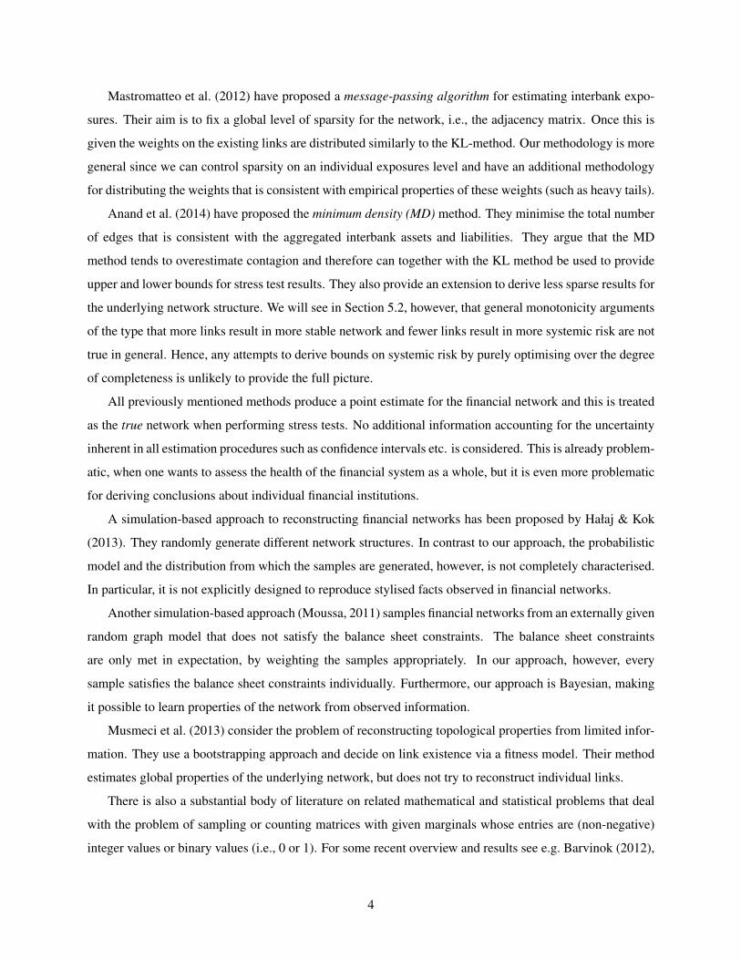
Figure 1: Survival function of the out-degree distribution of 10 simulated instances of the unconditionalbasic model (5) with n = 100 and pij = 0.3I(i 6= j).
Model parameters are two matrices: p ∈ [0, 1]n×n, where pij is the probability of the existence of a directed
edge from i to j, and λ ∈ (0,∞)n×n, which governs the distribution of the weights given that an edge exists.
Figure 1 shows an illustration of the out-degree distribution for a homogeneous choice of p.
We assume that we observe the following from the basic model (5):
r(L) = l, c(L) = a, L ≡ L∗, (6)
i.e., we only observe the row sums and column sums (l, a) and some elements of the liabilities matrix given
by L∗, the liabilities matrix L is not directly observable.
Our main interest lies in the distribution of some functional h of L (h(L)) conditional on l, a, L∗. For
example, we consider in Section 5.1 functions h that compute the vector of default indicators.
The distribution of h(L)|l, a, L∗ it not available in closed form; however it can be approximated using
MCMC methods. Indeed, the relatively simple form of the model (including the choice of an exponential
distribution of the existing liabilities) allows us to construct a Gibbs sampler (Section 4.1), for which we
need to compute certain conditional distributions.
It is a very flexible model. We will consider two setups in later examples, but other choices are possible:
In Section 5.3.1 we consider a homogeneous setup in which pij = pI(i 6= j) and λij = λ for fixed p and
λ; the resulting adjacency matrix is then essentially a classical Erdos-Renyi graph. In Section 5.3.2 we will
consider core-periphery models where the elements of the parameter matrices are not identical.
3.2 IdentifiabilityThe matrices p and λ cannot be fully identified merely by observing the row and column sums. Specif-
ically, the following proposition shows that in the minimal observation setting p cannot be identified from
row and column sums by showing that for any (reasonable) matrix p there exits a matrix of rate parameters
λ = (λij) s.t.∑n
i=1 E(Lij) = aj and∑n
j=1 E(Lij) = lj .
Proposition 3.1. Let l, a ∈ (0,∞)n with A =∑n
i=1 li =∑n
i=1 ai and ai + li < A ∀i. Let p ∈ [0, 1]n×n
8
with pij > 0 ∀i 6= j, diag(p) = 0. Then
∃(λij) such that ∀j :
n∑i=1
E(Lij) = aj and ∀i :
n∑j=1
E(Lij) = li.
A proof is given in Appendix A. The consequence of this lack of identifiability is that one needs to
impose some structure on p and λ, e.g. by setting these to specific values for the basic model or by assuming
a hierarchical model that makes assumptions about the network structure. This choice will be specific to the
application under consideration.
3.3 Hierarchical modelsThe basic model can be embedded into a larger Bayesian model, where the matrices p and λ are them-
selves random quantities. This allows incorporation of various features that one might observe in empirical
data (heavy or light tailed distribution etc.). Making p random allows us to model a wide range of degree
distributions including power laws. Making λ random in such a larger model gives us great flexibility on the
distribution of the liabilities. Indeed, a large range of important probability distributions can be character-
ized by exponential mixture models. An important result in this context is Bernstein’s theorem, which states
that every completely monotone probability density function is a mixture of exponential distributions (Feld-
mann & Whitt, 1997, Theorem 3.1.). For example, the Pareto II distribution (which can be heavy-tailed)
is a Gamma mixture of exponential distributions (Harris, 1968), see also Section 4.2 of the Supporting
Document.
We consider the following hierarchical model in which we assume that p and λ are influenced by some
underlying random parameter θ. In addition to (5), we assume
θ ∼ π(θ),
(pij , λij)i,j∈N = f(θ),(7)
where π is an a-priori distribution on θ and f is a given function. We will explore two examples of such
hierarchical models in the following.
3.3.1 Conjugate distribution model
This model assumes that all components of p (apart from the diagonal) and all components from λ are
equal but random. More precisely, we set θ = (p, λ) and assume
p ∼ Beta(α, β), λ ∼ Gamma(γ, δ),
pij = pI(i 6= j), λij = λ, i, j ∈ N ,
for some parameters α, β, γ, δ. The prior on p, λ is flexible and brings advantages in constructing samplers
as the conditional distribution of p|L follows a Beta distribution and λ|L follows a Gamma distribution.
A tiered financial network in which subsets of banks are assumed to be similar can be defined by parti-
tioning the matrix L and using independent models of the above type for each element of the partition.
9
3.3.2 Fitness model
Fitness models (see e.g. Caldarelli et al., 2002; Servedio et al., 2004) have mainly been used to model
undirected non-weighted networks. Typically, each node i is equipped with a random “fitness” xi (whose
pdf we denote by ρ) and links between nodes with fitness xi and xj are formed with probability f(xi, xj)
for a given function f . Several choices for f and ρ have been proposed, giving rise to different degree
distributions. In particular, power laws for the degree distributions can be obtained (Servedio et al., 2004).
A popular choice for f is the product of the (potentially transformed) fitnesses, i.e. f(xi, xj) = g(xi)g(xj)
for some function g. This structure limits the expected degree of the largest bank. Since we want to have the
possibility of one bank having connections to a large number of banks we do not use a product structure.
Our model will be a fitness model in which every bank i has an underlying fitness xi which influences
both its propensity to generate links (via p) as well as the size of its links (via λ). The model allows for a
power law for the number of links of banks (the degree distribution) as well as for the interbank liabilities
of a bank. This is motivated by empirical studies of interbank networks which have found power law
distributions for the degree distribution and the weights (see e.g. Boss et al., 2004).
Our model assumes that the fitness has an Exponential distribution with rate 1, i.e. ρ(x) = exp(−x)I(x ≥
0). Furthermore, we assume that the link function depends on the two fitnesses only through the sum of the
two fitnesses, i.e. f(xi, xj) = f(xi + xj) for a suitable function f . The precise model is as follows.
Xi ∼ Exp(1), i ∈ N ,
pij = f(Xi +Xj)I{i 6=j}, i 6= j ∈ N ,
λij = G−1ζ,η(exp(−Xi)) +G−1
ζ,η(exp(−Xj)) i, j ∈ N ,
(ζ, η) ∼ π(ζ, η),
(8)
where π is a suitable prior distribution, G−1ζ,η is the quantile function of a Gamma distribution with shape
parameter ζ > 0 and scale parameter η > 0 and
f(x) :=
β(γβ
)1−exp(−x) (1− log
(γβ
)exp(−x)
), if α = −1,
β (ξ + (1− ξ)e−x)1
α+1
{1 + 1
α+11−ξ
ξex+1−ξ
}, if α 6= −1,
(9)
where ξ := (γ/β)α+1, 0 < β < γ ≤ 1 and α < 0. We need to ensure 0 ≤ f(x) ≤ 1. Straightforward
calculations show that this is satisfied for α ≤ −2, but that for α > −2 we get the additional constraints:
if α ∈ (−2, 0) \ {−1} : γ/β ≤ (α+ 2)1
α+1 ; if α = −1 : γ/β ≤ e.
The link function f has been constructed such that the degree distribution exhibits a power law in the
sense that the pdf of the expected out-degree of a node at k is proportional to kα, where the distribution of
the expected out-degree is the distribution of the random variable dout(X), with X ∼ Exp(1) and
dout(x) = (n− 1)
∫ ∞0
f(x+ z)e−zdz.
10
0 20 40 60 80 100
0.0
0.2
0.4
0.6
0.8
1.0
k
P(d
eg>
=k)
(α,β,γ)
− 2.5,0.05,1− 2.5,0.2,1− 2.5,0.2,0.6− 2.5,0.5,1− 1,0.2,0.6− 1,0.5,1
5 10 20 50 100
2e−
042e
−03
2e−
022e
−01
k
log(
dens
ity m
ean
degr
ee(k
))
(α,β,γ)
− 2.5,0.05,1− 2.5,0.2,1− 2.5,0.2,0.6− 2.5,0.5,1− 1,0.2,0.6− 1,0.5,1
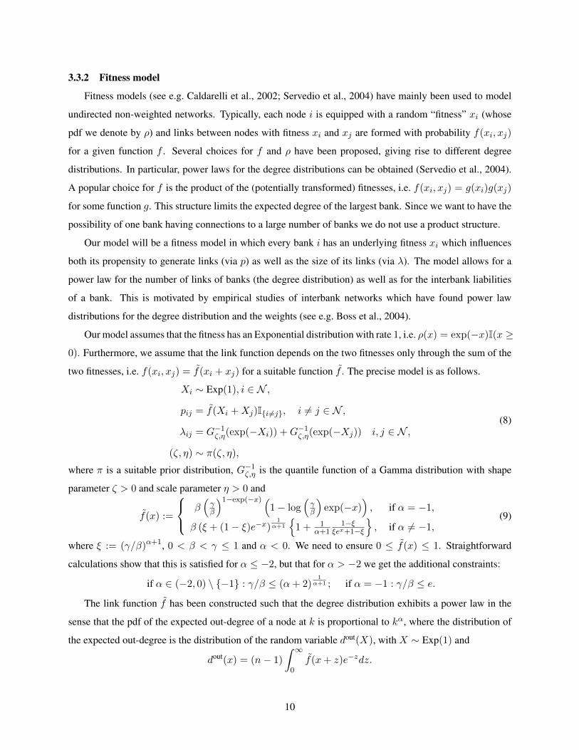
Figure 2: Survival function (left) and log-log plot of the pdf (right) of the distribution of the expectedout-degree for the fitness model with n = 100 nodes and various choices of parameters.
0 20 40 60 80 100
0.0
0.2
0.4
0.6
0.8
1.0
k
P(d
eg>
=k)
out−degree distributions
expectedrealised
1e+00 1e+02 1e+04 1e+06
1e−
041e
−03
1e−
021e
−01
1e+
00
x
P(L
ij≥
x)distribution of Lij
expected, conditional on Lij > 0realised, unconditional
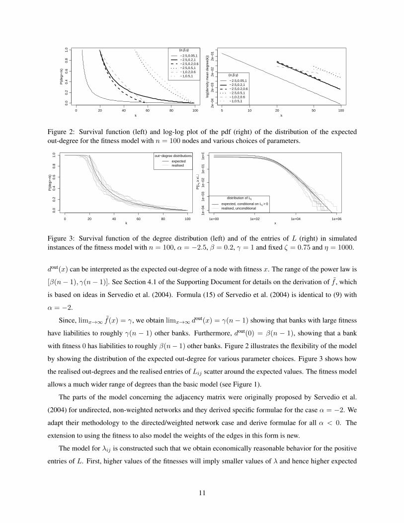
Figure 3: Survival function of the degree distribution (left) and of the entries of L (right) in simulatedinstances of the fitness model with n = 100, α = −2.5, β = 0.2, γ = 1 and fixed ζ = 0.75 and η = 1000.
dout(x) can be interpreted as the expected out-degree of a node with fitness x. The range of the power law is
[β(n− 1), γ(n− 1)]. See Section 4.1 of the Supporting Document for details on the derivation of f , which
is based on ideas in Servedio et al. (2004). Formula (15) of Servedio et al. (2004) is identical to (9) with
α = −2.
Since, limx→∞ f(x) = γ, we obtain limx→∞ dout(x) = γ(n− 1) showing that banks with large fitness
have liabilities to roughly γ(n − 1) other banks. Furthermore, dout(0) = β(n − 1), showing that a bank
with fitness 0 has liabilities to roughly β(n− 1) other banks. Figure 2 illustrates the flexibility of the model
by showing the distribution of the expected out-degree for various parameter choices. Figure 3 shows how
the realised out-degrees and the realised entries of Lij scatter around the expected values. The fitness model
allows a much wider range of degrees than the basic model (see Figure 1).
The parts of the model concerning the adjacency matrix were originally proposed by Servedio et al.
(2004) for undirected, non-weighted networks and they derived specific formulae for the case α = −2. We
adapt their methodology to the directed/weighted network case and derive formulae for all α < 0. The
extension to using the fitness to also model the weights of the edges in this form is new.
The model for λij is constructed such that we obtain economically reasonable behavior for the positive
entries of L. First, higher values of the fitnesses will imply smaller values of λ and hence higher expected
11
liabilities. This is because G−1ζ,η(e
−x) is decreasing in x.
Second, our model for Lij conditional on being positive is a mixture of exponentials as the distribution
on the fitness induces a mixture distribution on the λij . Our particular choice leads to heavy tails for this
distribution. Conditional on the parameters (ζ, η), we have G−1ζ,η(e
−X) ∼ Gamma(ζ, η) for X ∼ Exp(1)
because e−X has uniform distribution on (0, 1) and because applying the quantile function to a U(0, 1)
distributed random variable gives a random variable having this quantile function. Thus the rate parameter
λij is the sum of two independent Gamma distributed random variables and hence a Gamma distributed
random variable with shape parameter 2ζ and scale parameter η. A Gamma mixture of Exponentials has
Pareto II distribution (Harris, 1968). Hence, the distribution of a randomly selectedLij is for large arguments
close to the cdf of a Pareto II distribution with shape parameter 2ζ and scale parameter 1/η. I.e. for such
an Lij and x > 0, P(Lij > x) ≈ (1 + ηx)−2ζ (if β = γ = 1, this is the exact distribution). We provide
details on this in Section 4.2 of the Supporting Document. Boss et al. (2004) observe a power law in the
interbank liabilities of the Austrian interbank market with a power around−1.87. We can choose ζ to match
any power of interest. Hence, the priori model assumption is reasonable in the context of empirical data.
Third, when considering pairs of banks with very different fitnesses, the large bank essentially deter-
mines the link existence probability (to be high), and the small bank determines the weight (to be small).
Indeed, consider two banks, one with a high fitness xi and one with a low fitness xj . The high fitness xi
will lead to a high link existence probability. The small fitness xj leads to the transformed value e−xj being
large, implying a large corresponding quantile of the Gamma distribution. Hence, there is a large summand
in the definition of the corresponding λij which is resulting in a low expected weight. We would not obtain
this behaviour if we were to add the fitnesses before transforming to the desired Gamma distribution.
We have designed the specific fitness model such that it has many desirable economic features. Our
Bayesian framework can easily accommodate alternative choice for the distribution of the fitness ρ, the link
existence probabilities f or the relationship between the fitnesses and the rate parameter λ.
4 SamplingWe show how an MCMC algorithm (more precisely, a Gibbs-sampler) can be used to sample from the
conditional distribution of the liabilities matrix given its row and column sums (l, a) and known entries.
These samples can then be plugged into functionals of interest for systemic risk assessment, e.g., to work
out the distribution of the number of banks defaulting or the probability of the default of a specific bank. We
consider the basic model before extending the resulting methodology for hierarchical models.
In addition to the theoretical derivation of the samplers, we provide a simulation study in Section 1 of
the Supporting Document which shows that our samplers are sampling from the correct distribution and that
the implementation provided in the R package systemicrisk works.
12

To diagnose convergence of MCMC samplers, a large number of methods have been developed, see e.g.
Plummer et al. (2006). We demonstrate some of these methods in Section 2 of the Supporting Document.
4.1 A Gibbs sampler for the basic modelA large number of algorithms for sampling from matrices conditionally on their row and column sums
have been proposed; the introduction contains a short overview. Most algorithms are constructed for count
data, i.e., all entries are either assumed to be binary or to be nonnegative integers. These methods are not
directly applicable in our setting for two reasons. First, we are assuming that our entries are coming from
absolutely continuous random variables with a point mass at 0. Second, certain elements can be set to fixed
values - in the minimal observation setting the diagonal is set to 0.
We develop a Gibbs sampler to generate samples from the liabilities matrix conditional on the observed
row and column sums. The key idea of a Gibbs sampler is to iteratively update one or several components
of the entire parameter vector by sampling them from their joint conditional distribution given the other
components of the parameter vector. Often, components of the parameter vector are updated individually,
but sometimes it is necessary or more efficient to update several components of the parameter vector jointly.
By repeating these updating steps one constructs a Markov Chain whose distribution converges to the target
distribution as the number of updating steps tends to infinity.
In practice, the results are reported based on a single run of the chain. Often a burn-in period is used,
i.e., one discards the first few samples. Afterwards one often does not use every sample but only every
δth sample for a suitable nonnegative integer δ. This thinning reduces the autocorrelation of the retained
samples. See Robert & Casella (2004) for background regarding MCMC methods and the Gibbs sampler.
In our case the parameter vector is the matrix L. The MCMC sampler will then produce a sequence of
matrices L1, L2, . . . and for our quantity of interest we use the approximation
E[h(L)|l, a] ≈ 1
N
N∑i=1
h(Liδ+b),
where N is the number of samples to use in the estimation, b is the length of the burn-in period and δ ∈ N
defines the amount of thinning employed. For a specific application, a reasonable ambition is to ensure that
the N dependent samples being produced from the MCMC chain are equivalent to an independent sample
of size, say, N/10. An appropriate amount of thinning can be set using pilot runs of the chain together
with estimates of the componentwise effective sample size (using e.g. the CODA package (Plummer et al.,
2006)). Our R-package includes a function that determines the thinning in this way. As default burn-in we
use b equivalent to 10% of the overall effort.
4.1.1 Components that can be updated
For the construction of a Gibbs sampler, updating individual components of L is not useful, as condi-
tionally on the row and column sums and the other values of L, the individual components are uniquely
13

Li1j1 Li1j2
Li2j1 Li2j2
Li1j1 Li1j2
Li2j2Li2j3
Li3j3 Li3j1
Li1j1 Li1j2
Li2j2 Li2j3
Li3j3Li3j4
Li4j4 Li4j1
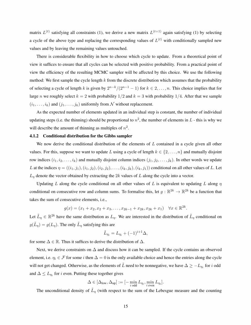
Figure 4: Illustration of submatrices to be updated via a Gibbs step (left-to-right): k = 2, 3, 4.
determined. Thus we need to jointly update a subset of the components of L.
The smallest possible update where we can hope to have some degrees of freedom would be based on
updating a 2x2 submatrix, see the left matrix in Figure 4. Conditioning on the row and column sums and
all other components of L is equivalent to conditioning on the row and column sum of the original 2x2
submatrix of L. This gives 4− 1 = 3 side conditions (the total row and column sums automatically match),
leaving one degree of freedom if none of the elements of the submatrix are fixed.
Performing Gibbs updates of 2x2 submatrices will not be enough to iterate through the space of possible
liabilities matrices. To see this, consider Example 2.4. Here, any 2x2 submatrix contains at least one element
of the diagonal. Thus Gibbs updates of 2x2 matrices leave L unchanged.
This is why we use more general updates - as subcomponents to update we use cycles given by an
integer k ∈ {2, . . . , n} and mutually disjoint row indices (i1, i2, . . . , ik) and mutually disjoint column
indices (j1, j2, . . . , jk). We update L at the indices
η := ((i1, j1), (i1, j2), (i2, j2), . . . , (ik, jk), (ik, j1))
conditional on all other values of L. We refer to such a cycle as a cycle of length k. A cycle of length k
contains the indices of 2k elements of L. Figure 4 illustrates submatrices that can be updated along a cycle.
Conditioning on the row and column sums of the current subelements of L is equivalent to conditioning
on other values of L. Thus we can implement a Gibbs sampler if we are able to sample from such a subset
of values with given row and column sums. We discuss how to do this in Section 4.1.2.
We need to initialise the chain with a matrix L that satisfies r(L) = l and c(L) = a. To generate
such a matrix we could use a maximum flow algorithm on the flow network constructed in the proof of
Theorem 2.3. This would result in a very sparse matrix. This would potentially lead to the need to use a
long burn-in phase. To reduce this problem, we first sample an Erdos-Renyi random matrix L with degree
existence probability roughly equal to the the average degree distribution of the unconditional model and
with r(L) ≤ l and c(L) ≤ a (which is easy to ensure). We then use the maximum flow-algorithm on the
remaining row and column sum and add the resulting matrix to L.
Our implementation of the Gibbs sampler uses the above update steps as follows. Based on a given
14
matrix L(t) satisfying all constraints (1), we derive a new matrix L(t+1) again satisfying (1) by selecting
a cycle of the above type and replacing the corresponding values of L(t) with conditionally sampled new
values and by leaving the remaining values untouched.
There is considerable flexibility in how to choose which cycle to update. From a theoretical point of
view it suffices to ensure that all cycles can be selected with positive probability. From a practical point of
view the efficiency of the resulting MCMC sampler will be affected by this choice. We use the following
method: We first sample the cycle length k from the discrete distribution which assumes that the probability
of selecting a cycle of length k is given by 2n−k/(2n−1 − 1) for k ∈ 2, . . . , n. This choice implies that for
large n we roughly select k = 2 with probability 1/2 and k = 3 with probability 1/4. After that we sample
(i1, . . . , ik) and (j1, . . . , jk) uniformly from N without replacement.
As the expected number of elements updated in an individual step is constant, the number of individual
updating steps (i.e. the thinning) should be proportional to n2, the number of elements in L - this is why we
will describe the amount of thinning as multiples of n2.
4.1.2 Conditional distribution for the Gibbs sampler
We now derive the conditional distribution of the elements of L contained in a cycle given all other
values. For this, suppose we want to update L using a cycle of length k ∈ {2, . . . , n} and mutually disjoint
row indices (i1, i2, . . . , ik) and mutually disjoint column indices (j1, j2, . . . , jk). In other words we update
L at the indices η = ((i1, j1), (i1, j2), (i2, j2), . . . , (ik, jk), (ik, j1)) conditional on all other values of L. Let
Lη denote the vector obtained by extracting the 2k values of L along the cycle into a vector.
Updating L along the cycle conditional on all other values of L is equivalent to updating L along η
conditional on consecutive row and column sums. To formalise this, let g : R2k → R2k be a function that
takes the sum of consecutive elements, i.e.,
g(x) = (x1 + x2, x2 + x3, . . . , x2k−1 + x2k, x2k + x1) ∀x ∈ R2k.
Let Lη ∈ R2k have the same distribution as Lη. We are interested in the distribution of Lη conditional on
g(Lη) = g(Lη). The only Lη satisfying this are
Lηi = Lηi + (−1)i+1∆,
for some ∆ ∈ R. Thus it suffices to derive the distribution of ∆.
Next, we derive constraints on ∆ and discuss how it can be sampled. If the cycle contains an observed
element, i.e. ηi ∈ F for some i then ∆ = 0 is the only available choice and hence the entries along the cycle
will not get changed. Otherwise, as the elements of L need to be nonnegative, we have ∆ ≥ −Lηi for i odd
and ∆ ≤ Lηi for i even. Putting these together gives
∆ ∈ [∆low,∆up] := [−mini odd
Lηi ,mini even
Lηi ].
The unconditional density of Lη (with respect to the sum of the Lebesgue measure and the counting
15
measure at 0) is
f(Lη) =2k∏i=1
((1− pηi)I(Lηi = 0) + pηiI(Lηi > 0)ληi exp(−ληiLηi)
). (10)
When conditioning on g(Lη) = g(Lη) we need to be careful as we are working with a measure consisting
of both continuous and discrete parts. The discrete part will come into play only for ∆ ∈ {∆low,∆up} and
the continuous part for ∆ ∈ (∆low,∆up).
It turns out (Appendix B.1) that if only one zero is contained in the boundary cases Llow,i = Lηi +
(−1)i+1∆low, i ∈ {1, 2, . . . , 2k} or Lup,i = Lηi + (−1)i+1∆up i ∈ {1, 2, . . . , 2k} then the conditional dis-
tribution of ∆ is supported on both {∆low,∆up} as well as on the continuous part (∆low,∆up). However, if
more than one zero is contained in Llow or Lup then the entire probability mass is concentrated on the bound-
ary case with the highest number of zeros and the probability of the intermediate case ∆ ∈ (∆low,∆up) is
zero. If the number of zeros is identical for both boundary cases then the conditional distribution is split
between these cases.
Conditional on the intermediate case ∆ ∈ (∆low,∆up), using density transformation, we show in Section
B.2 that the distribution of ∆ conditional on g(Lη) = g(Lη) and Lηi 6= 0, i = 1, . . . , 2k is given by what we
call a “restricted generalised exponential distribution” with rate parameter∑2k
i=1(−1)i+1ληi meaning that
its density on the support ∆ ∈ (∆low,∆up) is proportional to
exp
[−
(2k∑i=1
(−1)i+1ληi
)∆
].
The generalisation compared to the conventional exponential distribution is that the rate parameter need not
be positive. This is possible because ∆ has bounded support (∆low,∆up).
One of the consequences of the above is that an updating step can delete edges as well as create edges
and change weights of existing edges.
These considerations together with working out all conditional probabilities via Bayes formula lead to
Algorithm 1. Some remarks on it follow. The function f∗ defined in line 2 is related to the density f defined
in (10) in the sense that f∗(∆) = f(Lη + s∆). If, for at least one component of the cycle, the probability of
a link is exactly 0 then there is no flexibility in the update and thus the original matrix needs to be returned;
this is done in line 4. Line 7 computes the number of zeros arising in the boundary cases. If this is at most
one, then both the boundary cases {∆low,∆up} as well as the intermediate case (∆low,∆up) are part of the
possible support. In lines 10–12 we sample among these cases with the appropriate probabilities. Lines
18–21 deal with the case that more than one value of zero is possible in this update step. In this case the
boundary case with the highest number of 0s dominates the other cases, see Appendix B.
Within our R-package, Algorithm 1 is implemented in C++. This allows for fast execution of a large
number of steps. For example, in a setup with roughly 30% of the elements of L being positive in a network
16

Algorithm 1: Sampling of a cycle conditional on row and column sums in the model (5)
Input: k ∈ N, i, j ∈ {1, . . . , n}k, L ∈ [0,∞)n×n, p ∈ [0, 1]n×n, λ ∈ (0,∞)n×n
1 η = ((i1, j1), (i1, j2), (i2, j2), . . . , (ik, jk), (ik, j1)); s = (1,−1, 1, . . . , 1,−1) ∈ R2k
2 Let f∗ : R→ R,∆ 7→2k∏i=1
[I(Lηi + si∆ = 0)(1− pηi) + I(Lηi + si∆ > 0)pηiληie
−ληi (Lηi+si∆)].
3 For every ∆ ∈ R, let L∆ ∈ Rn×n be defined by L∆ηi = Lηi + si∆, i = 1, . . . , 2k and by being equal
to L for all other components.4 if ∃i : pηi = 0 then return L5 ∆up = mini=2,4,...,2k Lηi ; ∆low = −mini=1,3,...,2k−1 Lηi6 if ∆low = ∆up then return L7 n0
up = #{i even : Lηi = ∆up}; n0low = #{i odd : Lηi = −∆low}
8 if n0up ≤ 1 and n0
low ≤ 1 then9 λ =
∑i ληisi
10 if λ = 0 then p∗ = (∆up −∆low)f∗(12(∆up + ∆low))
11 else p∗ = λ−1(
exp[λ
∆up−∆low2
]− exp
[−λ∆up−∆low
2
])f∗(1
2(∆up + ∆low))
12 Sample x from {1, 2, 3} with probabilities ξf∗(∆low), ξp∗, ξf∗(∆up) whereξ = (f∗(∆low) + p∗ + f∗(∆up))−1
13 if x=1 then return L∆low
14 if x=2 then15 Sample ∆ from the extended exponential distribution restricted to (∆low,∆up) with rate λ16 return L∆
17 if x=3 then return L∆up
18 else19 if n0
up > n0low then return L∆up
20 if n0low > n0
up then return L∆low
21 if n0low = n0
up then with probability f∗(∆low)f∗(∆low)+f∗(∆up) return L∆low ; otherwise return L∆up
with n = 100 nodes, 5 · 106 cycle updates take about one second on a single core of an Intel Core i7-860
CPU with a clock speed of 2.8 GHz.
4.1.3 Gibbs moves can reach all admissible matrices
By construction, a Gibbs sampler automatically has the correct invariant distribution. Full convergence
proofs usually rely on showing Harris recurrence (Robert & Casella, 2004), which is essentially the require-
ment that the entire space is explored repeatedly. In this section we make a step towards such a proof by
showing that, under conditions, the Gibbs sampler can move from a matrix L1 to any other matrix L2.
Theorem 4.1. Let a, l ∈ [0,∞)n. Suppose that L1, L2 ∈ [0,∞)n×n are such that for L = L1 and L = L2
the following conditions are satisfied:
(i) (correct row/column sums) r(L) = l, c(L) = a.
(ii) (L consistent with p) ∀i, j ∈ N : Lij > 0⇒ pij > 0.
(iii) (L connected along rows/columns) The undirected graph G = (V,E) with vertices
17

V = {r1, . . . , rn, c1, . . . , cn} and edges E = {(ri, cj) : (i, j) /∈ F , Lij > 0} is connected.
(iv) (no positive ties) ∀i, j, i∗, j∗ ∈ N : Lij = Li∗j∗ 6= 0 implies i = i∗, j = j∗.
Then there exists a sequence of moves by the Gibbs sampler in Algorithm 1 that transforms L1 to L2.
The proof can be found in Appendix A. Condition (iii) considers the bipartite graph with nodes corre-
sponding to all rows and all columns in which a row is connected to a column if the corresponding entry in L
is positive. Connectedness of this graph, i.e. that all nodes can be reached from any node, can be efficiently
checked for a given matrix L using e.g. depth first search (Cormen et al., 1990).
One can see that condition (iii) is implied for all L satisfying (i) by the following condition on a and l:
∀I, J ⊆ N :
∑i∈I
li =∑j∈J
aj =⇒ I = J = N or I = J = ∅
. (11)
Fully checking (11) is usually only feasible for small n as it is similar to the NP-hard equal-subset-sum
problem, see e.g. Woeginger & Yu (1992). Condition (iv) is satisfied with probability one in the models that
we consider, e.g. for models (5) and (8).
4.2 MCMC samplers for hierarchical modelsIn the hierarchical model the unknown parameters are L and θ. To sample from (θ, L)|a, l, L∗ in this
joint model we can again use a Gibbs sampler (or a Metropolis within Gibbs sampler). As θ directly defines
the matrices p and λ, the updates used in the basic model can be used to update components of L. Updating
components of θ will depend on the specific choice of θ and f . Below we give some examples.
The model of Section 3.3.1 has been specifically set up such that the priors for p (a Beta distribution)
and λ (a Gamma distribution) are conjugate priors for the model generating L (the indicators I(Lij > 0)
are independent Bernoulli random variables with parameter p and Lij conditional on Lij > 0 follows an
Exponential distribution with parameter λ). Hence, (p, λ)|L is given by independent Beta and Gamma
distributions with appropriately updated parameter values.
For the fitness model in Section 3.3.2 we use Metropolis-Hastings updates to update θ. As these are
straightforward extensions of our basic sampler we present the details in Section 3 of the Supporting Docu-
ment.
5 Applications to systemic risk assessment5.1 Stress testing a financial network
We now use our methodology for stress testing. We assume that in addition to the row and column sums
of L we also observe the external assets a(e) ∈ [0,∞)n and the liabilities to entities outside the interbank
network l(e) ∈ [0,∞)n. Table 1 illustrates a simple balance sheet based on this. The vector of total liabilities
is lall := l(e) + r(L) ∈ Rn and the vector of net worths is w = w(L, a(e), l(e)) = a(e) + c(L) − lall. If
wi ≥ 0, the net worth corresponds to the book value of bank i’s equity.
18
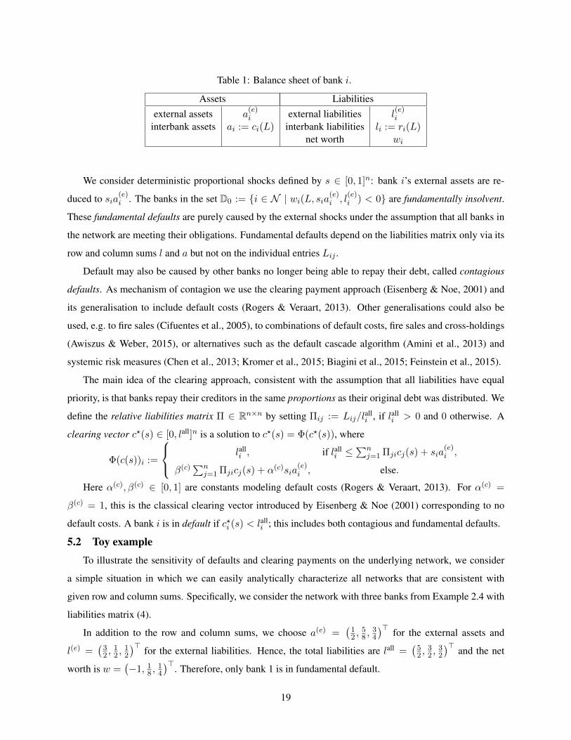
Table 1: Balance sheet of bank i.
Assets Liabilitiesexternal assets a
(e)i external liabilities l
(e)i
interbank assets ai := ci(L) interbank liabilities li := ri(L)net worth wi
We consider deterministic proportional shocks defined by s ∈ [0, 1]n: bank i’s external assets are re-
duced to sia(e)i . The banks in the set D0 := {i ∈ N | wi(L, sia(e)
i , l(e)i ) < 0} are fundamentally insolvent.
These fundamental defaults are purely caused by the external shocks under the assumption that all banks in
the network are meeting their obligations. Fundamental defaults depend on the liabilities matrix only via its
row and column sums l and a but not on the individual entries Lij .
Default may also be caused by other banks no longer being able to repay their debt, called contagious
defaults. As mechanism of contagion we use the clearing payment approach (Eisenberg & Noe, 2001) and
its generalisation to include default costs (Rogers & Veraart, 2013). Other generalisations could also be
used, e.g. to fire sales (Cifuentes et al., 2005), to combinations of default costs, fire sales and cross-holdings
(Awiszus & Weber, 2015), or alternatives such as the default cascade algorithm (Amini et al., 2013) and
systemic risk measures (Chen et al., 2013; Kromer et al., 2015; Biagini et al., 2015; Feinstein et al., 2015).
The main idea of the clearing approach, consistent with the assumption that all liabilities have equal
priority, is that banks repay their creditors in the same proportions as their original debt was distributed. We
define the relative liabilities matrix Π ∈ Rn×n by setting Πij := Lij/lalli , if lall
i > 0 and 0 otherwise. A
clearing vector c?(s) ∈ [0, lall]n is a solution to c?(s) = Φ(c?(s)), where
Φ(c(s))i :=
lalli , if lall
i ≤∑n
j=1 Πjicj(s) + sia(e)i ,
β(c)∑n
j=1 Πjicj(s) + α(c)sia(e)i , else.
Here α(c), β(c) ∈ [0, 1] are constants modeling default costs (Rogers & Veraart, 2013). For α(c) =
β(c) = 1, this is the classical clearing vector introduced by Eisenberg & Noe (2001) corresponding to no
default costs. A bank i is in default if c?i (s) < lalli ; this includes both contagious and fundamental defaults.
5.2 Toy exampleTo illustrate the sensitivity of defaults and clearing payments on the underlying network, we consider
a simple situation in which we can easily analytically characterize all networks that are consistent with
given row and column sums. Specifically, we consider the network with three banks from Example 2.4 with
liabilities matrix (4).
In addition to the row and column sums, we choose a(e) =(
12 ,
58 ,
34
)> for the external assets and
l(e) =(
32 ,
12 ,
12
)> for the external liabilities. Hence, the total liabilities are lall =(
52 ,
32 ,
32
)> and the net
worth is w =(−1, 1
8 ,14
)>. Therefore, only bank 1 is in fundamental default.
19
0.0 0.2 0.4 0.6 0.8 1.0
0.77
0.78
0.79
0.80
x
(a) Sum of clearing payments / sum of total liabilities
0.0 0.2 0.4 0.6 0.8 1.0
x
bank 1
bank 2
bank 3
(b) Default range
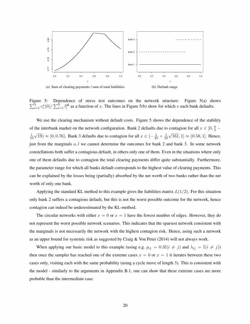
Figure 5: Dependence of stress test outcomes on the network structure: Figure 5(a) shows∑3i=1 c
?i (0)/
∑3i=1 l
alli as a function of x. The lines in Figure 5(b) show for which x each bank defaults.
We use the clearing mechanism without default costs. Figure 5 shows the dependence of the stability
of the interbank market on the network configuration. Bank 2 defaults due to contagion for all x ∈ [0, 65 −
110
√19) ≈ [0, 0.76). Bank 3 defaults due to contagion for all x ∈ (− 1
20 + 120
√161, 1] ≈ (0.58, 1]. Hence,
just from the marginals a, l we cannot determine the outcomes for bank 2 and bank 3. In some network
constellations both suffer a contagious default, in others only one of them. Even in the situations where only
one of them defaults due to contagion the total clearing payments differ quite substantially. Furthermore,
the parameter range for which all banks default corresponds to the highest value of clearing payments. This
can be explained by the losses being (partially) absorbed by the net worth of two banks rather than the net
worth of only one bank.
Applying the standard KL method to this example gives the liabilities matrix L(1/2). For this situation
only bank 2 suffers a contagious default, but this is not the worst possible outcome for the network, hence
contagion can indeed be underestimated by the KL-method.
The circular networks with either x = 0 or x = 1 have the fewest number of edges. However, they do
not represent the worst possible network scenarios. This indicates that the sparsest network consistent with
the marginals is not necessarily the network with the highest contagion risk. Hence, using such a network
as an upper bound for systemic risk as suggested by Craig & Von Peter (2014) will not always work.
When applying our basic model to this example (using e.g. pij = 0.3I(i 6= j) and λij = I(i 6= j))
then once the sampler has reached one of the extreme cases x = 0 or x = 1 it iterates between these two
cases only, visiting each with the same probability (using a cycle move of length 3). This is consistent with
the model - similarly to the arguments in Appendix B.1, one can show that these extreme cases are more
probable than the intermediate case.
20
5.3 Empirical exampleIn the following we demonstrate how our methodology can be applied to empirical data. To do this, we
use data from banks that took part in the European Banking Authority’s (EBA) 2011 stress test4.
For every bank, the total assets ai + a(e)i , the interbank assets ai and the net worth wi (i.e., the Tier 1
capital) are available. Hence, the external assets a(e)i are available as the difference between the total assets
and the interbank assets. The interbank liabilities li are not provided in the data set. Some empirical studies
based on these data assumed li = ai ∀i ∈ N , see e.g. Chen et al. (2014) and Glasserman & Young (2015).
We will assume that li is a slightly perturbed version of ai to ensure that condition (11) is satisfied. In
particular, we set li := r(
(ai + εi)∑nj=1 aj∑n
j=1(aj+εj)
), i ∈ {1, . . . , n− 1}, and ln :=
∑ni=1 ai −
∑n−1i=1 li, where
r(·) is the rounding function to 1 decimal place and ε1, . . . , εn are independent realisations from a normal
distribution with mean 0 and standard deviation 100. Throughout this example we use one fixed realisation
for the li. Using this assumption, the external liabilities are given by l(e)i = (ai + a(e)i )− wi − li.
We look at a subset of the EBA stress test data containing eleven German banks as in Chen et al. (2014).
The corresponding balance sheet data are provided in Section 5 of the Supporting Document. The EBA
stress test data set contains the total interbank assets for each bank and total interbank assets that a given
bank has from banks in a specific country. To construct a closed network between the eleven banks, we only
use interbank assets from other German banks (rather than the total interbank assets across all countries).
We use the simplifying assumption that these interbank assets are from banks within the network, whereas
they will partially be from other German banks besides the 11 banks that we are considering. All other
assets are considered to be external assets in our analysis, even though parts of them are interbank assets
from banks that are not part of the network that we consider.
The data set allows us to study default behaviour in a heterogeneous network, which is rarely done in the
existing literature. Nevertheless, given the above simplifying assumptions, the results should be considered
an illustration of our methodology rather than specific information about the banks involved.
Initially all banks are solvent. We then apply a deterministic shock to the external assets of all eleven
banks in the network by considering the shocked external assets sia(e)i with si = 0.97∀i ∈ N . This
shock causes the fundamental default of four banks: DE017, DE022, DE023, DE024. We then use our new
methodology to determine the posteriori default probabilities for the remaining seven banks.
5.3.1 Basic model - homogeneous network assumption
Initially we assume that all link probabilities pij are identical, i.e., pij = p ∀i 6= j ∈ N and pii = 0∀i ∈
N . We consider probabilities p ∈ {0.2, 0.3, . . . , 0.9, 1}. We do not consider probabilities smaller than 0.2
since to satisfy the 2n− 1 = 21 side conditions we need at least a fraction of 21/(121− 11) ≈ 0.191 of the
4See http://www.eba.europa.eu/risk-analysis-and-data/eu-wide-stress-testing/2011/results
21
0.2 0.4 0.6 0.8 1.0
0.00
0.05
0.10
0.15
p
●
●
●
●
●
●●
● ●
DE020
●
●
●
●
●
●
●
●
●
DE025
●
●
●
●● ● ● ● ●
DE028
(a) Clearing with α(c) = 1, β(c) = 1
0.2 0.4 0.6 0.8 1.0
0.0
0.2
0.4
0.6
0.8
1.0
p
●●
● ● ● ● ● ● ●
DE018
●
●
●
●●
● ● ● ●
DE019●
●
●●
●● ● ● ●
DE020
●●
●
●
● ●●
● ●
DE021
●
●
●
●
●●
●● ●
DE025
● ● ●●
●
●
●
●
●
DE027
●
●
●
●
●●
● ● ●
DE028
(b) Clearing with α(c) = 1, β(c) = 0.7
0.2 0.4 0.6 0.8 1.0
0.0
0.2
0.4
0.6
0.8
1.0
p
●
●
●●
●● ● ● ●
DE018
●● ● ● ● ● ● ● ●
DE019 ●● ● ● ● ● ● ● ●
DE020
●●
●
●●
●●
● ●
DE021
●●
●●
●● ● ● ●
DE025
● ● ● ● ●●
●●
●
DE027
●
●●
● ● ● ● ● ●
DE028
(c) Clearing with α(c) = 0.9, β(c) = 1
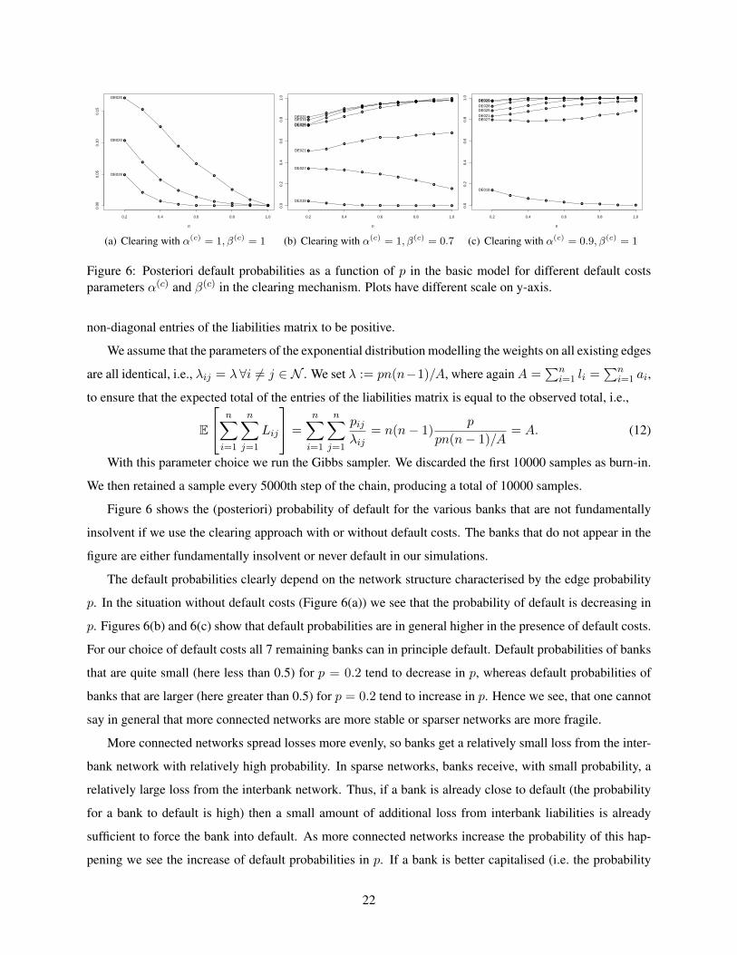
Figure 6: Posteriori default probabilities as a function of p in the basic model for different default costsparameters α(c) and β(c) in the clearing mechanism. Plots have different scale on y-axis.
non-diagonal entries of the liabilities matrix to be positive.
We assume that the parameters of the exponential distribution modelling the weights on all existing edges
are all identical, i.e., λij = λ ∀i 6= j ∈ N . We set λ := pn(n−1)/A, where againA =∑n
i=1 li =∑n
i=1 ai,
to ensure that the expected total of the entries of the liabilities matrix is equal to the observed total, i.e.,
E
n∑i=1
n∑j=1
Lij
=n∑i=1
n∑j=1
pijλij
= n(n− 1)p
pn(n− 1)/A= A. (12)
With this parameter choice we run the Gibbs sampler. We discarded the first 10000 samples as burn-in.
We then retained a sample every 5000th step of the chain, producing a total of 10000 samples.
Figure 6 shows the (posteriori) probability of default for the various banks that are not fundamentally
insolvent if we use the clearing approach with or without default costs. The banks that do not appear in the
figure are either fundamentally insolvent or never default in our simulations.
The default probabilities clearly depend on the network structure characterised by the edge probability
p. In the situation without default costs (Figure 6(a)) we see that the probability of default is decreasing in
p. Figures 6(b) and 6(c) show that default probabilities are in general higher in the presence of default costs.
For our choice of default costs all 7 remaining banks can in principle default. Default probabilities of banks
that are quite small (here less than 0.5) for p = 0.2 tend to decrease in p, whereas default probabilities of
banks that are larger (here greater than 0.5) for p = 0.2 tend to increase in p. Hence we see, that one cannot
say in general that more connected networks are more stable or sparser networks are more fragile.
More connected networks spread losses more evenly, so banks get a relatively small loss from the inter-
bank network with relatively high probability. In sparse networks, banks receive, with small probability, a
relatively large loss from the interbank network. Thus, if a bank is already close to default (the probability
for a bank to default is high) then a small amount of additional loss from interbank liabilities is already
sufficient to force the bank into default. As more connected networks increase the probability of this hap-
pening we see the increase of default probabilities in p. If a bank is better capitalised (i.e. the probability
22

of it defaulting is small) then a relatively large loss from the interbank network is needed to cause default.
More connected networks only lead to a relatively small loss for each bank from the interbank network -
this is why for better capitalised banks the default probability is decreasing in p.
For comparison purpose we have run the three different clearing mechanisms presented in Figure 6 on
the network that one obtains from minimising the Kullback-Leibler divergence. We used the code provided
in Temurshoev et al. (2013). The resulting network is complete. Without default costs (as in Figure 6(a))
all remaining 7 banks survive, for α(c) = 1, β(c) = 0.7 (as in Figure 6(b)) only bank DE018 and DE027
survive and for α(c) = 0.9, β(c) = 1 (as in Figure 6(c)) only bank DE018 survives. Here those banks whose
default probabilities tend to (almost) zero in the basic model as p goes to 1 turn out to be the survivors under
the KL method. Those banks that have higher default probabilities under the basic model assumption are
categorised as defaults under the KL method.
5.3.2 Basic model - tiered network assumption
Several empirical studies have found that financial networks exhibit tiering or some core-periphery struc-
ture, see e.g. Craig & Von Peter (2014) for the German interbank market. Motivated by this we now consider
situations in which not all edge probabilities pij are identical.
Following (Nier et al., 2007, Section 6), we assume that there are n(l) large banks and n(s) small banks
such that n(l) + n(s) = n. The probability p(l) that a large bank is connected to other banks (both large or
small) is assumed to be higher than the probability p(s) that small banks are connected to each other, i.e.
0 ≤ p(s) ≤ p(l) ≤ 1. Nier et al. (2007) argue that to make a meaningful comparison between an Erdos-Renyi
network with link probability p(ER) ∈ [0, 1] and a tiered network with p(s) ≤ p(l) one should require that the
expected number of links stays the same. This can be obtained by fixing n(l), n(s), p(l), p(ER) and setting
p(s) =n(n− 1)p(ER) − n(l)(n− 1)p(l) − n(l)n(s)p(l)
n(s)(n(s) − 1). (13)
Let I(s), I(l) ⊆ N denote the sets of indices corresponding to small and large banks, respectively, let pii = 0
∀i ∈ N and for all i 6= j let
pij =
p(l), if {i, j} ∩ I(l) 6= ∅,
p(s), if {i, j} ⊆ I(s).
For the parameters of the exponential distribution we choose λ = λij =∑nµ=1
∑nν=1 pµν
A ∀i 6= j, which is
consistent with the considerations in (12).
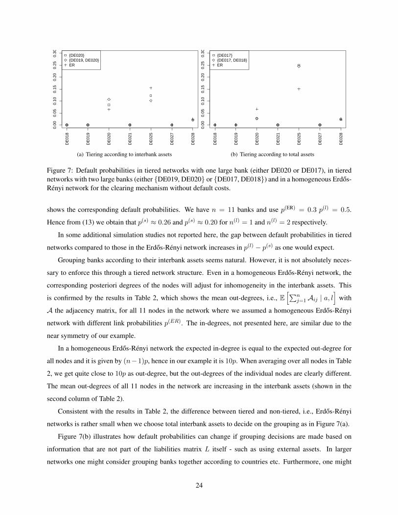
In the following we use two different criteria to decide on the tiered structure: total interbank assets and
total assets. The results are presented in Figure 7. The first network has bank DE020 as the only large bank.
The second has banks DE019 and DE020 as the only large banks (according to interbank assets). Figure
7(a) contains the corresponding default probabilities. The third tiered network uses bank DE017 as the only
large bank. The fourth uses DE017 and DE018 as large banks (according to total assets). Figures 7(b) and
23
0.00
0.05
0.10
0.15
0.20
0.25
0.30
DE
018
DE
019
DE
020
DE
021
DE
025
DE
027
DE
028
{DE020}{DE019, DE020}ER
(a) Tiering according to interbank assets
0.00
0.05
0.10
0.15
0.20
0.25
0.30
DE
018
DE
019
DE
020
DE
021
DE
025
DE
027
DE
028
{DE017}{DE017, DE018}ER
(b) Tiering according to total assets
Figure 7: Default probabilities in tiered networks with one large bank (either DE020 or DE017), in tierednetworks with two large banks (either {DE019, DE020} or {DE017, DE018}) and in a homogeneous Erdos-Renyi network for the clearing mechanism without default costs.
shows the corresponding default probabilities. We have n = 11 banks and use p(ER) = 0.3 p(l) = 0.5.
Hence from (13) we obtain that p(s) ≈ 0.26 and p(s) ≈ 0.20 for n(l) = 1 and n(l) = 2 respectively.
In some additional simulation studies not reported here, the gap between default probabilities in tiered
networks compared to those in the Erdos-Renyi network increases in p(l) − p(s) as one would expect.
Grouping banks according to their interbank assets seems natural. However, it is not absolutely neces-
sary to enforce this through a tiered network structure. Even in a homogeneous Erdos-Renyi network, the
corresponding posteriori degrees of the nodes will adjust for inhomogeneity in the interbank assets. This
is confirmed by the results in Table 2, which shows the mean out-degrees, i.e., E[∑n
j=1Aij | a, l]
with
A the adjacency matrix, for all 11 nodes in the network where we assumed a homogeneous Erdos-Renyi
network with different link probabilities p(ER). The in-degrees, not presented here, are similar due to the
near symmetry of our example.
In a homogeneous Erdos-Renyi network the expected in-degree is equal to the expected out-degree for
all nodes and it is given by (n−1)p, hence in our example it is 10p. When averaging over all nodes in Table
2, we get quite close to 10p as out-degree, but the out-degrees of the individual nodes are clearly different.
The mean out-degrees of all 11 nodes in the network are increasing in the interbank assets (shown in the
second column of Table 2).
Consistent with the results in Table 2, the difference between tiered and non-tiered, i.e., Erdos-Renyi
networks is rather small when we choose total interbank assets to decide on the grouping as in Figure 7(a).
Figure 7(b) illustrates how default probabilities can change if grouping decisions are made based on
information that are not part of the liabilities matrix L itself - such as using external assets. In larger
networks one might consider grouping banks together according to countries etc. Furthermore, one might
24
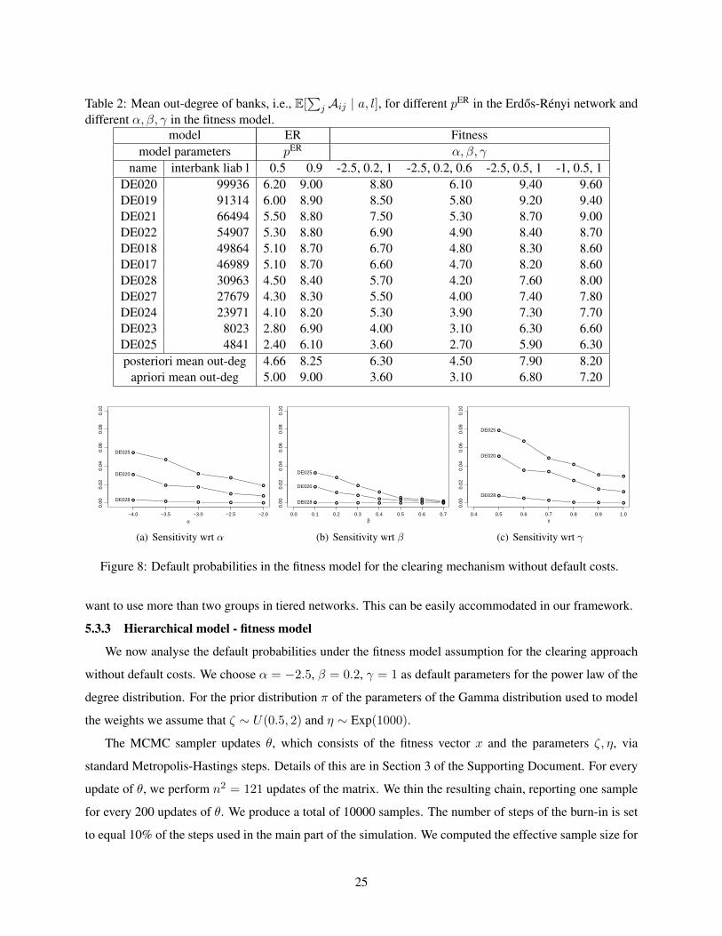
Table 2: Mean out-degree of banks, i.e., E[∑
j Aij | a, l], for different pER in the Erdos-Renyi network anddifferent α, β, γ in the fitness model.
model ER Fitnessmodel parameters pER α, β, γ
name interbank liab l 0.5 0.9 -2.5, 0.2, 1 -2.5, 0.2, 0.6 -2.5, 0.5, 1 -1, 0.5, 1DE020 99936 6.20 9.00 8.80 6.10 9.40 9.60DE019 91314 6.00 8.90 8.50 5.80 9.20 9.40DE021 66494 5.50 8.80 7.50 5.30 8.70 9.00DE022 54907 5.30 8.80 6.90 4.90 8.40 8.70DE018 49864 5.10 8.70 6.70 4.80 8.30 8.60DE017 46989 5.10 8.70 6.60 4.70 8.20 8.60DE028 30963 4.50 8.40 5.70 4.20 7.60 8.00DE027 27679 4.30 8.30 5.50 4.00 7.40 7.80DE024 23971 4.10 8.20 5.30 3.90 7.30 7.70DE023 8023 2.80 6.90 4.00 3.10 6.30 6.60DE025 4841 2.40 6.10 3.60 2.70 5.90 6.30posteriori mean out-deg 4.66 8.25 6.30 4.50 7.90 8.20
apriori mean out-deg 5.00 9.00 3.60 3.10 6.80 7.20
●
●●
●●
−4.0 −3.5 −3.0 −2.5 −2.0
0.00
0.02
0.04
0.06
0.08
0.10
α
DE020
●
●
●
●
●
DE025
● ● ● ● ●DE028
(a) Sensitivity wrt α
●
●●
● ● ● ●
0.0 0.1 0.2 0.3 0.4 0.5 0.6 0.7
0.00
0.02
0.04
0.06
0.08
0.10
β
DE020
●
●
●
●
● ●●
DE025
● ● ● ● ● ● ●DE028
(b) Sensitivity wrt β
●
● ●
●
●●
0.4 0.5 0.6 0.7 0.8 0.9 1.0
0.00
0.02
0.04
0.06
0.08
0.10
γ
DE020
●
●
●
●
●●
DE025
●●
●● ● ●
DE028
(c) Sensitivity wrt γ
Figure 8: Default probabilities in the fitness model for the clearing mechanism without default costs.
want to use more than two groups in tiered networks. This can be easily accommodated in our framework.
5.3.3 Hierarchical model - fitness model
We now analyse the default probabilities under the fitness model assumption for the clearing approach
without default costs. We choose α = −2.5, β = 0.2, γ = 1 as default parameters for the power law of the
degree distribution. For the prior distribution π of the parameters of the Gamma distribution used to model
the weights we assume that ζ ∼ U(0.5, 2) and η ∼ Exp(1000).
The MCMC sampler updates θ, which consists of the fitness vector x and the parameters ζ, η, via
standard Metropolis-Hastings steps. Details of this are in Section 3 of the Supporting Document. For every
update of θ, we perform n2 = 121 updates of the matrix. We thin the resulting chain, reporting one sample
for every 200 updates of θ. We produce a total of 10000 samples. The number of steps of the burn-in is set
to equal 10% of the steps used in the main part of the simulation. We computed the effective sample size for
25

all components of L as well as well as for all elements of θ using the CODA package in R (Plummer et al.,
2006): the effective sample size was above 1000 for all simulation runs of this section. Further diagnostic
assessments, not reported here, did not flag any convergence problems.
Figure 8 shows the sensitivities of the default probabilities with respect to the parameters modelling the
degree distribution α, β, γ. The same banks that are at risk of defaulting (DE025, DE020, DE028) under the
basic model are also at risk of defaulting under the fitness model. Their default probabilities are in a similar
range under both modelling assumption. Default probabilities are decreasing as the power parameter α of
the degree distribution increases (note that α < 0). As we can see in Table 2 the smaller α the lower is
the corresponding mean out-degree in the network. This corresponds to higher default probabilities in this
example as it was the case under the basic modelling assumption. A similar effect can be observed when we
change the range parameters of the power law β and γ. Higher values of β imply a higher mean out-degree
of the network, see Table 2, and again we observe a decrease in default probabilities. Also higher values of
γ imply higher mean out-degrees and lower default probabilities in this example.
The ordering of the banks stays the same under both the basic model as well as the fitness model. The
larger the total interbank liabilities the larger the out-degree (and the larger the corresponding posteriori
fitness). Under the power law assumption we can influence the variability of the out-degrees with a small
number of parameters. If the range of the power law is quite narrow, i.e. β, γ are close together we obtain a
more homogeneous network; otherwise the out-degrees between the banks can vary substantially. This can
be further influenced by the choice of the power parameter α.
6 ConclusionWe have described mechanisms for generating liabilities matrices that are consistent with the marginal
constraints on the total liabilities and total assets of each bank in the network and satisfy some additional
properties as well. These additional properties are describing properties of the network structure that we
assume to be known or at least estimated from empirical data.
Instead of a fixed shock we could use a random shock. This can be easily accommodated in our method-
ology by sampling one or several different shocks for each sample of a liabilities matrix.
In practice, the data from different banks may be based on (slightly) different time points or use slightly
different accounting assumptions. Even the basic consistency condition∑n
i=1 ai =∑n
i=1 li will often not be
satisfied. To accommodate this our model could be extended by allowing for random errors in the observed
total interbank liabilities/assets. Details of this are outside the scope of this paper.
A ProofsProof of Theorem 2.3. We transform the problem of finding a liabilities matrix into a max-flow problem.
We use the terminology defined in Cormen et al. (1990). We may assume that the observed values in L∗ are
26
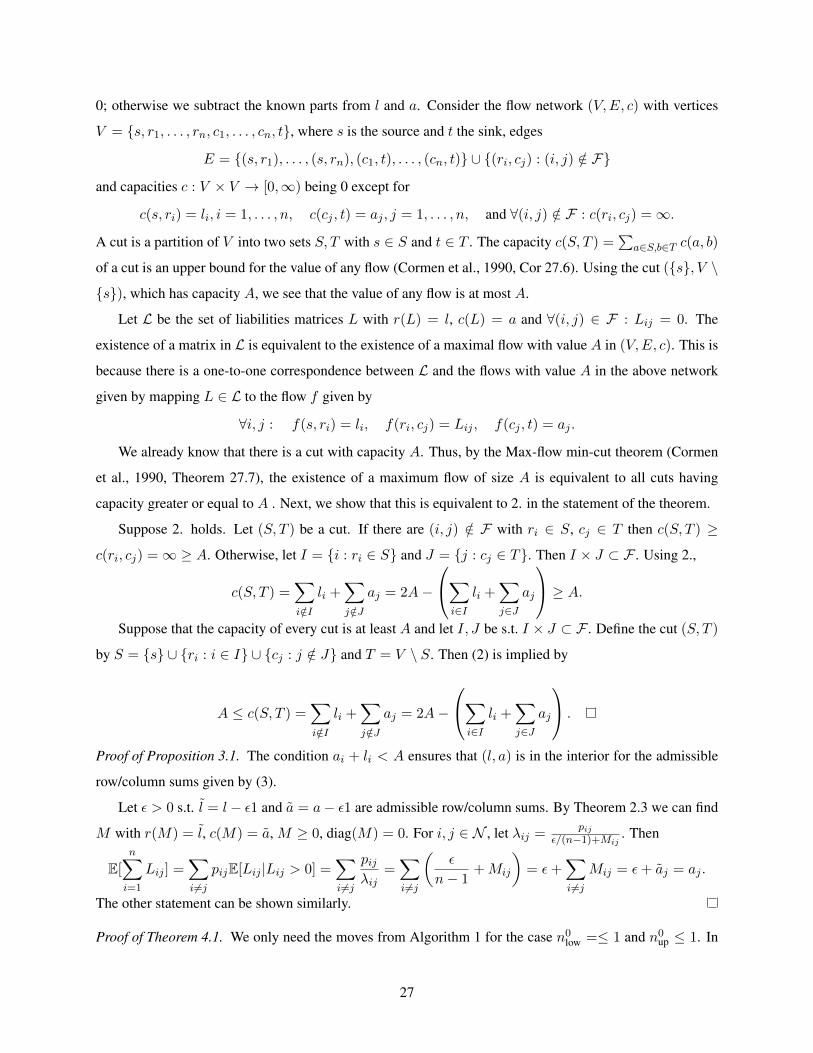
0; otherwise we subtract the known parts from l and a. Consider the flow network (V,E, c) with vertices
V = {s, r1, . . . , rn, c1, . . . , cn, t}, where s is the source and t the sink, edges
E = {(s, r1), . . . , (s, rn), (c1, t), . . . , (cn, t)} ∪ {(ri, cj) : (i, j) /∈ F}
and capacities c : V × V → [0,∞) being 0 except for
c(s, ri) = li, i = 1, . . . , n, c(cj , t) = aj , j = 1, . . . , n, and ∀(i, j) /∈ F : c(ri, cj) =∞.
A cut is a partition of V into two sets S, T with s ∈ S and t ∈ T . The capacity c(S, T ) =∑
a∈S,b∈T c(a, b)
of a cut is an upper bound for the value of any flow (Cormen et al., 1990, Cor 27.6). Using the cut ({s}, V \
{s}), which has capacity A, we see that the value of any flow is at most A.
Let L be the set of liabilities matrices L with r(L) = l, c(L) = a and ∀(i, j) ∈ F : Lij = 0. The
existence of a matrix in L is equivalent to the existence of a maximal flow with value A in (V,E, c). This is
because there is a one-to-one correspondence between L and the flows with value A in the above network
given by mapping L ∈ L to the flow f given by
∀i, j : f(s, ri) = li, f(ri, cj) = Lij , f(cj , t) = aj .
We already know that there is a cut with capacity A. Thus, by the Max-flow min-cut theorem (Cormen
et al., 1990, Theorem 27.7), the existence of a maximum flow of size A is equivalent to all cuts having
capacity greater or equal to A . Next, we show that this is equivalent to 2. in the statement of the theorem.
Suppose 2. holds. Let (S, T ) be a cut. If there are (i, j) /∈ F with ri ∈ S, cj ∈ T then c(S, T ) ≥
c(ri, cj) =∞ ≥ A. Otherwise, let I = {i : ri ∈ S} and J = {j : cj ∈ T}. Then I × J ⊂ F . Using 2.,
c(S, T ) =∑i/∈I
li +∑j /∈J
aj = 2A−
∑i∈I
li +∑j∈J
aj
≥ A.Suppose that the capacity of every cut is at least A and let I, J be s.t. I × J ⊂ F . Define the cut (S, T )
by S = {s} ∪ {ri : i ∈ I} ∪ {cj : j /∈ J} and T = V \ S. Then (2) is implied by
A ≤ c(S, T ) =∑i/∈I
li +∑j /∈J
aj = 2A−
∑i∈I
li +∑j∈J
aj
.
Proof of Proposition 3.1. The condition ai + li < A ensures that (l, a) is in the interior for the admissible
row/column sums given by (3).
Let ε > 0 s.t. l = l− ε1 and a = a− ε1 are admissible row/column sums. By Theorem 2.3 we can find
M with r(M) = l, c(M) = a, M ≥ 0, diag(M) = 0. For i, j ∈ N , let λij =pij
ε/(n−1)+Mij. Then
E[
n∑i=1
Lij ] =∑i 6=j
pijE[Lij |Lij > 0] =∑i 6=j
pijλij
=∑i 6=j
(ε
n− 1+Mij
)= ε+
∑i 6=j
Mij = ε+ aj = aj .
The other statement can be shown similarly.
Proof of Theorem 4.1. We only need the moves from Algorithm 1 for the case n0low =≤ 1 and n0
up ≤ 1. In
27
this case moves exist to all L∆ for ∆ ∈ [∆low,∆up]. These moves are reversible in the sense that if one can
move from L to L∆ then one can move from L∆ to L by using −∆ as increment.
Let S(L) = {(i, j) : Lij > 0} be the support of a matrix L. Let S = S(L1)∪S(L2) be the joint support
of L1 and L2. Let C be the set of matrices satisfying (i), (ii), (iii), (iv).
We first show that we can transform any L ∈ C with S(L) ⊂ S to a matrix in C with S(L) = S
using cycle moves. Suppose (i, j) ∈ S with Lij = 0. We construct a cycle move that gives a matrix in
C with S(L) ⊂ S where this entry is positive without creating additional zeros. Iteratively applying this
construction transforms L to a matrix that is positive on S.
As (i, j) ∈ S we have L1ij > 0 or L2
ij > 0 implying ri(L) = ri(L1) = ri(L
2) > 0. Hence, there exists
j∗ such that Lij∗ > 0. Similarly, there exists i∗ such that Li∗j > 0. By the connectedness of L, there exists
a simple path between (ri, cj∗) and (ri∗ , cj) along G. Together with (i, j) this defines a cycle that only has
one zero. As there are no tied positive value in L there is a unique smallest positive value ξ of L along this
cycle and we can use the cycle move with ∆ ∈ (0, ξ) chosen such that no positive ties are being created.
This will transform L into a matrix in C with (i, j) ∈ S.
Thus we can transform L1 into a positive matrix on S . As all of the steps are reversible, any matrix
L ∈ C with S(L) = S can be transformed into L2. It remains to construct transformations between matrices
in C with support S. Let L1 and L2 be two such matrices. Let D = L2 − L1. The following step reduces
the number of nonzero entries in D by at least 1. Repeated application removes the differences between L1
and L2, as there are only finitely many differences and as the step does not create new differences.
Let η1 = (i, j) be such that Dij < 0. Starting from η1, construct a path with ηi ∈ N 2 and ηi1 = ηi+11 for
odd i and ηi2 = ηi+12 for even i such that Dηi < 0 for odd i and Dηi > 0 for even i. As the row and column
sums of D are 0 it is always possible to extend this path by an additional element. Extend the path until,
for the first time, the first component or the second component repeats itself in non-adjacent elements of the
path i.e., if m is the current length of the path then for some j ≤ m − 2 we have (ηj1 = ηm1 , ηj1 6= ηj+11 )
or (ηj2 = ηm2 and ηj2 6= ηj+12 ). Then use the cycle (ηj , . . . , ηm) to remove the smallest value (in absolute
values) in D (denote the index of this element by b). To do this choose this element as the first element of
the cycle (reversing the cycle if necessary) and use ∆ = −Db.
B Conditional distribution on a cycleThis section provides details on the derivation of Algorithm 1. Suppose the current liabilities matrix isL.
Suppose we have a fixed cycle of length k with η determining the index pairs of the elements to be updated.
To ease notation, we use Li = Lηi , Li = Lηi , and similarly for p, λ. Let s = (1,−1, . . . , 1,−1) ∈ R2k.
28

B.1 Probability of the boundary cases and the intermediate caseWe work out the probability of the boundary cases ∆ ∈ {∆low,∆up} and the intermediate case ∆ ∈
(∆low,∆up). For this we compute the probability of a realisation in a neighbourhood of (Li + si∆)i=1,...,2k
for ∆ = ∆low,∆ = ∆up and ∆ ∈ (∆low,∆up) before letting the size of this neighbourhood go to 0.
First we consider the boundary case. Suppose ∆ ∈ {∆low,∆up}, then the exact value for Li would be
xi = Li + si∆, at least one of which is 0. The probability of all Li being at most ε > 0 away from xi is
P(|Li − xi| < ε, i = 1, . . . , 2k) =2k∏i=1
((1− pi)I(|xi| < ε) + pi
∫ xi+ε
(xi−ε)+
λie−λiydy
)= O
(ε#{i:xi 6=0}
)as ε→ 0, where x+ = max(x, 0) and #B is the number of elements in the set B. In particular, #{i : xi 6=
0} ≤ 2k − 1 and we might even sometimes have a strict inequality.
Next we consider the intermediate case ∆ ∈ (∆low,∆up). Suppose ∆low 6= ∆up, then for all ∆ ∈
(∆low,∆up), all xi(∆) = Li + si∆, i = 1, . . . , 2k will be positive, implying that only the absolutely
continuous part of the random variable is relevant in this case. Integrating out the one degree of freedom
given by ∆, one sees that the probability of Lη being close to (x1(∆), . . . , x2k(∆)) for some ∆ is
P(L1 − L1 ∈ (∆low,∆up), Li ∈ BL1−L1i (ε), i = 2, . . . , 2k) =
=
∫ L1+∆up
L1+∆low
2k∏i=2
(∫Bi(x1−L1,ε)
λie−λixidxi
)λ1e−λ1x1dx1 = O(ε2k−1)
as ε→ 0 where B∆i (ε) = (max(Li + si∆− ε, 0), Li + si∆ + ε).
Hence, if two or more 0s are produced in Lη for ∆ = ∆low or ∆ = ∆up then the boundary case
dominates the intermediate case (hence we have lines 18–21 in Algorithm 1). Otherwise, the probability
contributions of the boundary case and the intermediate case are of the same order and we sample among
these cases in lines 10–12 of Algorithm 1; for details of this see the next subsection.
B.2 The case where there is at most one 0 at the boundaryThe conditional distribution of L along the cycle η is concentrated on matrices of the form Lη+s∆ with
∆ ∈ [∆low,∆up]. This section considers the case #{i : Li + si∆up = 0} = #{i : Li + si∆low = 0} = 1.
We first work out the probability mass for the three cases ∆ = ∆low, ∆ ∈ (∆low,∆up) and ∆ = ∆up.
The probability mass for the boundary case ∆ = ∆low is f(Lη + s∆low) and for ∆ = ∆up is f(Lη + s∆up).
The total probability mass of the intermediate case ∆ ∈ (∆low,∆up) is∫(∆low,∆up)
f(Lη + s∆)d∆ =
∫(∆low,∆up)
2k∏i=1
piλie−λi(Li+si∆)d∆
=2k∏i=1
piλie−λi(Li+si∆)
∫(∆low,∆up)
e−λ(∆−∆)d∆ = f(Lη + s∆)
∫(∆low,∆up)
e−λ(∆−∆)d∆,
29
where ∆ =∆low+∆up
2 , λ =∑2k
i=1 λisi. If λ = 0 then this is f(Lη + s∆)(∆up −∆low), otherwise it is
f(Lη + s∆)− λ−1e−λ(∆−∆)|∆up∆low
= f(Lη + s∆)λ−1[eλ
∆up−∆low2 − e−λ
∆up−∆low2
].
Next, we work out the distribution of ∆ conditional on the intermediate case ∆ ∈ (∆low,∆up). Consider
the mapping g : R2k → R2k, g1(x) = x1−L1, gi(x) = xi−1 +xi. Then g(L) = (∆, L1 + L2, . . . , L2k−1 +
L2k). We are interested in the distribution of ∆ = g1(L) conditional on gi(L) = gi(L), i = 2, . . . , 2k.
Using standard density transformation, and the fact that g is a linear mapping where the matrix has
determinant 1, we get that the density ofM = g(L) is f(g−1(M)).′ Hence, conditionally on gi(L) = gi(L),
i = 2, . . . , 2k, the density of ∆ = g1(L) is proportional to
f(g−1(∆, L1 + L2, . . . , L2k−1 + L2k)) = f(L+ s∆) =
2k∏i=1
piλie−λi(Li+si∆) ∝ e−(
∑2ki=1 λisi)∆ = e−λ∆,
which is an extended exponential distribution with parameter λ restricted to the interval (∆low,∆up).
C AcknowledgmentsThe authors thank the editor, the associate editor, and the referees for their valuable comments.
ReferencesAmini, H., Cont, R. & Minca, A. (2013). Resilience to contagion in financial networks. Mathematical
Finance Early View.
Anand, K. (2015). The missing links - a global study on uncovering financial network structure from par-
tial data. Presentation slides available at http://www.risk.jbs.cam.ac.uk/news/events/other/2015/150909
financialriskandnetworktheory.html.
Anand, K., Craig, B. & Von Peter, G. (2014). Filling in the blanks: Network structure and interbank conta-
gion. Quantitative Finance 1–12.
Awiszus, K. & Weber, S. (2015). The joint impact of bankruptcy costs, fire sales and
cross-holdings on systemic risk in financial networks. Available at http://www.stochastik.uni-
hannover.de/fileadmin/institut/pdf/JointImpactPaper.pdf.
Bank of England (2015). The Bank of England’s approach to stress testing the UK banking system. Available
at http://www.bankofengland.co.uk/financialstability/Documents/stresstesting/2015/approach.pdf.
Barvinok, A. (2012). Matrices with prescribed row and column sums. Linear Algebra and its Applications
436, 820–844.
Biagini, F., Fouque, J.-P., Frittelli, M. & Meyer-Brandis, T. (2015). A unified approach to systemic risk
measures via acceptance sets. arXiv preprint arXiv:1503.06354 .
Boss, M., Elsinger, H., Summer, M. & Thurner 4, S. (2004). Network topology of the interbank market.
Quantitative Finance 4, 677–684.
Brualdi, R. A. (2006). Combinatorial matrix classes, vol. 13. Cambridge University Press.
30
Caldarelli, G., Capocci, A., De Los Rios, P. & Munoz, M. A. (2002). Scale-free networks from varying
vertex intrinsic fitness. Physical review letters 89, 258702.
Chen, C., Iyengar, G. & Moallemi, C. C. (2013). An axiomatic approach to systemic risk. Management
Science 59, 1373–1388.
Chen, N., Liu, X. & Yao, D. D. (2014). An optimization view of financial systemic risk modeling: The
network effect and the market liquidity effect. Available at SSRN: http://ssrn.com/abstract=2463545.
Cifuentes, R., Ferrucci, G. & Shin, H. S. (2005). Liquidity risk and contagion. Journal of the European
Economic Association 3, 556–566.
Cormen, T. T., Leiserson, C. E. & Rivest, R. L. (1990). Introduction to Algorithms. MIT Press.
Craig, B. & Von Peter, G. (2014). Interbank tiering and money center banks. Journal of Financial Interme-
diation 23, 322–347.
Degryse, H. & Nguyen, G. (2007). Interbank exposures: An empirical examination of contagion risk in the
Belgian banking system. International Journal of Central Banking 3, 123–171.
Diaconis, P., Sturmfels, B. et al. (1998). Algebraic algorithms for sampling from conditional distributions.
The Annals of Statistics 26, 363–397.
Eisenberg, L. & Noe, T. H. (2001). Systemic risk in financial systems. Management Science 47, 236–249.
Elsinger, H., Lehar, A. & Summer, M. (2006). Using market information for banking system risk assessment.
International Journal of Central Banking 2.
Elsinger, H., Lehar, A. & Summer, M. (2013). Network models and systemic risk assessment. Handbook on
Systemic Risk 1, 287–305.
Erdos, P. & Renyi, A. (1959). On random graphs I. Publicationes Mathematicae Debrecen 6, 290–297.
Feinstein, Z., Rudloff, B. & Weber, S. (2015). Measures of systemic risk. arXiv:1502.07961 .
Feldmann, A. & Whitt, W. (1997). Fitting mixtures of exponentials to long-tail distributions to analyze net-
work performance models. In INFOCOM’97. Sixteenth Annual Joint Conference of the IEEE Computer
and Communications Societies., Proceedings IEEE, vol. 3, 1096–1104.
Financial Stability Board & International Monetary Fund (2015). The financial crisis and information
gaps - sixth progress report on the implementation of the G-20 data gaps initiative. Available at
http://www.imf.org/external/np/g20/pdf/2015/6thprogressrep.pdf.
Glasserman, P. & Young, H. P. (2015). How likely is contagion in financial networks? Journal of Banking
& Finance 50, 383–399.
Hałaj, G. & Kok, C. (2013). Assessing interbank contagion using simulated networks. ECB Working Paper
Series, No 1506.
Haldane, A. (2015). On microscopes and telescopes. Speech available at
31

http://www.bankofengland.co.uk/publications/Pages/speeches/2015/812.aspx.
Harris, C. M. (1968). The Pareto distribution as a queue service discipline. Operations Research 16, 307–
313.
Hurd, T. R. (2015). Contagion! The spread of systemic risk in financial networks. Book in progress; available
from http://ms.mcmaster.ca/tom/tom.html.
Kromer, E., Overbeck, L. & Zilch, K. A. (2015). Systemic risk measures on general measurable spaces.
Available at SSRN: http://ssrn.com/abstract=2268105 or http://dx.doi.org/10.2139/ssrn.2268105.
Langfield, S., Liu, Z. & Ota, T. (2014). Mapping the UK interbank system. Journal of Banking & Finance
45, 288–303.
Mastromatteo, I., Zarinelli, E. & Marsili, M. (2012). Reconstruction of financial networks for robust esti-
mation of systemic risk. Journal of Statistical Mechanics: Theory and Experiment 2012, P03011.
Miller, J. W., Harrison, M. T. et al. (2013). Exact sampling and counting for fixed-margin matrices. The
Annals of Statistics 41, 1569–1592.
Mistrulli, P. E. (2011). Assessing financial contagion in the interbank market: Maximum entropy versus
observed interbank lending patterns. Journal of Banking & Finance 35, 1114–1127.
Moussa, A. (2011). Contagion and Systemic Risk in Financial. Ph.D. thesis, Columbia University.
Musmeci, N., Battiston, S., Caldarelli, G., Puliga, M. & Gabrielli, A. (2013). Bootstrapping topological
properties and systemic risk of complex networks using the fitness model. Journal of Statistical Physics
151, 720–734.
Nier, E., Yang, J., Yorulmazer, T. & Alentorn, A. (2007). Network models and financial stability. Journal of
Economic Dynamics and Control 31, 2033–2060.
Plummer, M., Best, N., Cowles, K. & Vines, K. (2006). CODA: Convergence diagnosis and output analysis
for MCMC. R news 6, 7–11.
Robert, C. & Casella, G. (2004). Monte Carlo statistical methods. 2 ed., Springer.
Rogers, L. C. G. & Veraart, L. A. M. (2013). Failure and rescue in an interbank network. Management
Science 59, 882–898.
Ryser, H. J. (1960). Matrices of zeros and ones. Bulletin of the American Mathematical Society 66, 442–464.
Servedio, V. D. P., Caldarelli, G. & Butta, P. (2004). Vertex intrinsic fitness: How to produce arbitrary
scale-free networks. Phys. Rev. E 70, 056126.
Snijders, T. A. (1991). Enumeration and simulation methods for 0–1 matrices with given marginals. Psy-
chometrika 56, 397–417.
Temurshoev, U., Miller, R. E. & Bouwmeester, M. C. (2013). A note on the GRAS method. Economic
Systems Research 25, 361–367.
32

Upper, C. (2011). Simulation methods to assess the danger of contagion in interbank markets. Journal of
Financial Stability 7, 111–125.
Upper, C. & Worms, A. (2004). Estimating bilateral exposures in the German interbank market: Is there a
danger of contagion? European Economic Review 48, 827–849.
Wells, S. J. (2004). Financial interlinkages in the United Kingdom’s interbank market and the risk of conta-
gion. Bank of England working paper.
Woeginger, G. J. & Yu, Z. (1992). On the equal-subset-sum problem. Information Processing Letters 42,
299–302.
Zaman, A. & Simberloff, D. (2002). Random binary matrices in biogeographical ecology - instituting a good
neighbor policy. Environmental and Ecological Statistics 9, 405–421.
33