Embed Size (px)
Citation preview
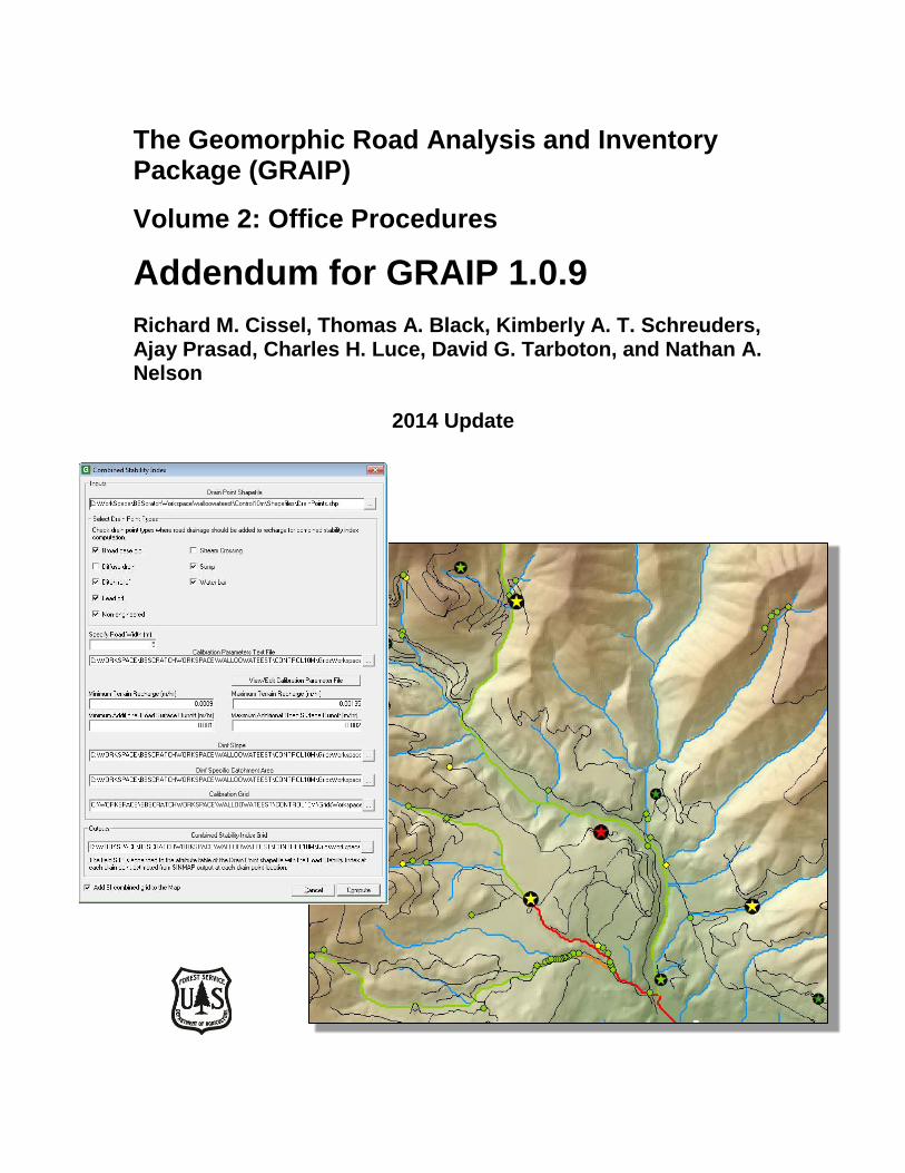
The Geomorphic Road Analysis and Inventory Package (GRAIP)
Volume 2: Office Procedures
Addendum for GRAIP 1.0.9
Richard M. Cissel, Thomas A. Black, Kimberly A. T. Schreuders, Ajay Prasad, Charles H. Luce, David G. Tarboton, and Nathan A. Nelson
2014 Update

The Geomorphic Road Analysis and Inventory Package (GRAIP) Volume 2: Office Procedures
ADDENDUM FOR GRAIP 1.0.9 UPDATE
Richard M. Cissel, Thomas A. Black, Kimberly A. T. Schreuders, Ajay Prasad, Charles
H. Luce, David G. Tarboton, and Nathan A. Nelson
Current as of March 17, 2014
For GRAIP v. 1.0.9 and field data dictionary INVENT 5.0
Support
We are interested in feedback. If you find errors, have suggestions, or are interested in any later versions contact:
David G. Tarboton
Utah State University
4110 Old Main Hill
Logan, UT 84322-4110 USA
Email: [email protected]
http://www.neng.usu.edu/cee/faculty/dtarb/
index.html
Tom Black
Rocky Mountain Research Station
322 East Front Street, Suite 401
Boise, Idaho, 83702 USA
Email: [email protected]
http://www.fs.fed.us/GRAIP/index.shtml
Commercial Endorsement Disclaimer
The use of trade, firm, or corporation names in the publication is for the information and
convenience of the reader. Such use does not constitute an official endorsement or
approval by the U.S. Department of Agriculture of any product or service to the exclusion
of others that may be suitable.
Table of Contents
INTRODUCTION .............................................................................................................. 1 SECTION I: ABOUT GRAIP 1.0.9 ................................................................................... 1
What Has Changed? ........................................................................................................ 1 Minor Changes to Processes ........................................................................................... 2
Changes to the Manual Text and Figures ....................................................................... 5 SECTION II: REPLACEMENT INSTRUCTIONS ........................................................... 7
Preprocessing Shapefiles ................................................................................................ 7 Running TauDEM ......................................................................................................... 15 Mass Wasting Potential Analysis.................................................................................. 21
Appendix D: Attribute Table Field Name Explanations............................................... 35 Release Notes .................................................................................................................... 37
References ......................................................................................................................... 38
Addendum to The Geomorphic Road Analysis And Inventory Package (GRAIP) Volume 2: Office Procedures
1
INTRODUCTION
This update to GRAIP 1.0.9 addresses a number of concerns with GRAIP 1.0.8.
There were some issues that resulted in slightly inaccurate modeling results or the
addition of extra steps to the process. If you are comparing data that you modeled with
GRAIP 1.0.8 to newer data that will be modeled with GRAIP 1.0.9, then you should re-
run the GRAIP 1.0.8 data with the updated version of GRAIP. Changes made are not
expected to significantly affect model results, however, so there may not be a need to
update old data that is not being used for comparison with new data.
GRAIP 1.0.9 is compatible with Windows 7, as well as previous versions at least
as old as Windows XP. However, it is not compatible with ArcGIS 10, and requires
ArcGIS 9 (9.3.1 is the most recent). GRAIP is written in the Visual Basic language,
which is not compatible with ArcGIS 10. In order to update GRAIP to run in the current
version of ArcGIS, the program will need to be re-written in another programming
language; this update is expected to be available late in 2014 or in 2015.
The purpose of this Addendum is to address and explain these changes (Section I:
About GRAIP 1.0.9), and to update the GRAIP office manual (Cissel et al. 2012) where
there are new processes or significant changes to old processes (Section II: Replacement
Instructions). In addition to a detailed explanation of the changes made, Section I covers
some other minor updates to processes and additional information not covered in the
GRAIP office manual. The instructions in Section II should be used in place of those in
the office manual.
SECTION I: ABOUT GRAIP 1.0.9
This section discusses the changes made to GRAIP in detail, presents a brief how-
to for avoiding the use of Hawth’s Tools, which is defunct, discusses DEMs in more
detail than is present in the office manual, and addresses how to integrate this information
with that available in the office manual.
What Has Changed?
There were a number of changes made with the update to GRAIP 1.0.9, both to
increase usability and to correct some program errors. Perhaps the most substantial, the
way in which the range of a road line is calculated (that is, ), which is
used in the calculation of sediment production for each road segment, has been changed
so that it is more accurate. Previously, this function referred to ArcGIS Zonal Statistics to
find the range, which uses the minimum and maximum elevation values along the road.
The change was made so that GRAIP now calculates the range based on the DEM cell
value at the end points of each road line segment, independently of Zonal Statistics. This
results in a more realistic range for the road lines. There are no changes to the procedure
that result from this.
Addendum to The Geomorphic Road Analysis And Inventory Package (GRAIP) Volume 2: Office Procedures
2
The next major change is to the method in which the Combined Stability Index
function works. Previously, this function included water that drained to stream crossings
and diffuse points when it modeled the risk of shallow landslides due to roads. Since
these drain points do not behave in the same way as the others when it comes to
landslides, there was a complicated set of steps that had to be performed to remove the
water that drained to those points from consideration. The Combined Stability Index
function has been modified so that the user can choose which drain points to include, and
stream crossings (regular and excavated) and diffuse points are excluded by default. This
saves a lot of time, and the simplified process is included in this Addendum (Section II).
The other changes to the model were:
- A modification to the sediment routing in streams to fix the error where sediment
may have been routed upstream on some flat slope stream segments.
- A change to the Stream Blocking Index (SBI) function so that only culverts (steel,
aluminum, plastic, cement, etc.) are now included in the calculation of SBI, and
bridges, fords, and log culverts are excluded.
- The specific sediment (SpecSed in the stream network shapefile) is now
calculated correctly, using sediment accumulation (SedAccum) converted to Mg
and downstream contributing area (DS_Cont_Ar) converted to km2.
- An improvement to the resampling method used in the Resample DEM step so
that it now uses the cubic convolution method instead of the nearest neighbor
method.
- The addition of the discharge location to the DrainPoints shapefile (the
DischargeT field).
Each of these do not require any change to the procedure. Finally, an overland flow
distance from the drain point to the closest stream field has been added to the DrainPoints
shapefile (in m; DistToStre). This requires an extra step be taken when TauDEM is run,
and that section has been updated and included in Section II.
Minor Changes to Processes
Previously, GRAIP has depended on Hawth’s Tools to generate outlet points at
road-stream intersections in order to split the stream lines at the intersections so that
sediment is not routed upstream of the road. Hawth’s has been out of date for a number of
years, and its replacement does not have the same functionality. There are two methods
that can be used to generate the Outlets shapefile. These instructions apply to the
Preprocessing section of the office manual, starting on p.89.
First, you can use XTools Pro, which has a license available for Forest Service
computers, but otherwise is not free, and has a function that will do this in one step.
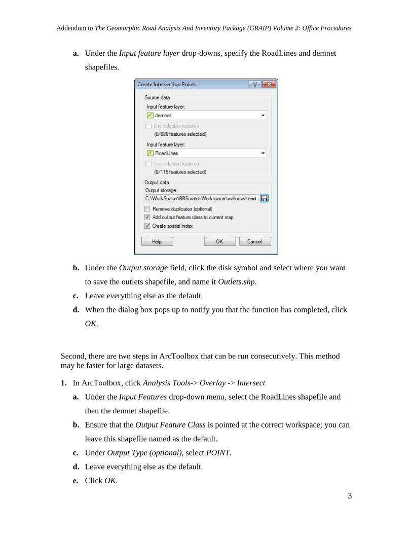
1. In the XTools toolbar, click the XTools Pro drop-down -> Layer Operations-> Create
Intersection Points
Addendum to The Geomorphic Road Analysis And Inventory Package (GRAIP) Volume 2: Office Procedures
3
a. Under the Input feature layer drop-downs, specify the RoadLines and demnet
shapefiles.
b. Under the Output storage field, click the disk symbol and select where you want
to save the outlets shapefile, and name it Outlets.shp.
c. Leave everything else as the default.
d. When the dialog box pops up to notify you that the function has completed, click
OK.
Second, there are two steps in ArcToolbox that can be run consecutively. This method
may be faster for large datasets.
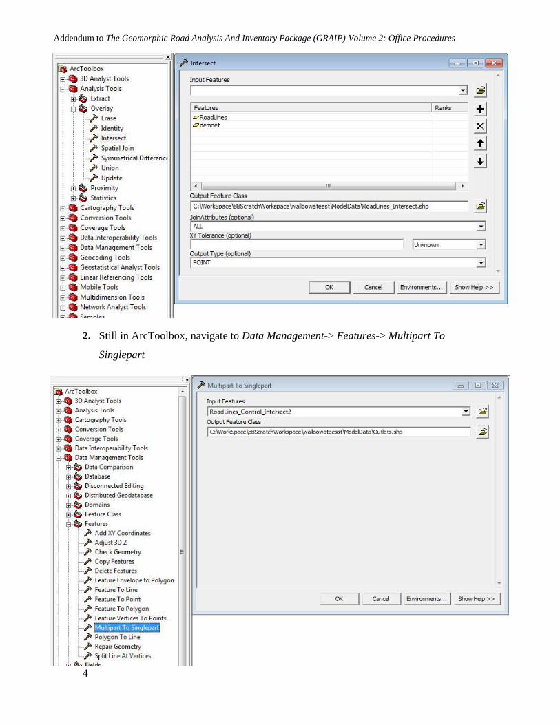
1. In ArcToolbox, click Analysis Tools-> Overlay -> Intersect
a. Under the Input Features drop-down menu, select the RoadLines shapefile and
then the demnet shapefile.
b. Ensure that the Output Feature Class is pointed at the correct workspace; you can
leave this shapefile named as the default.
c. Under Output Type (optional), select POINT.
d. Leave everything else as the default.
e. Click OK.
Addendum to The Geomorphic Road Analysis And Inventory Package (GRAIP) Volume 2: Office Procedures
4
2. Still in ArcToolbox, navigate to Data Management-> Features-> Multipart To
Singlepart

Addendum to The Geomorphic Road Analysis And Inventory Package (GRAIP) Volume 2: Office Procedures
5
a. Under Input Features, select the shapefile you created in step 1.
b. Under Output Features, ensure that the new shapefile will be saved to the correct
workspace, and rename it Outlets.shp.
3. Click OK.
4. You can delete the shapefile that was created during step 1.
The DEM that you use has an effect on the data outputs. The National Map
website is currently the main easy source for DEMs for anywhere in the United States.
DEMs downloaded from the National Map are in one degree blocks, projected into the
GCS North American NAD83 coordinate system, and are in decimal degrees (as opposed
to meters). For most locations, there are multiple options for the resolution of the DEM.
One arc second corresponds to about 30 m, depending on latitude, and most DEMs were
created as one arc second natively. This is the best resolution to use most of the time. If
your watershed overlaps more than one of these one-degree blocks, you will need to
mosaic those DEMs using the Mosaic To New Raster function under ArcToolbox-> Data
Management Tools-> Raster-> Raster Dataset, using 32_BIT_FLOAT in the Pixel type
(optional) field. Once the DEM is mosaicked, it should be projected into the UTM
coordinate system using the method in the manual (p. 33), with the exception of leaving
the Output cell size (optional) field as whatever the default is (usually some number
between 25 and 27 in the northern parts of the continental U.S.). In general, the more you
change a DEM, the less accurate it will be. Though the DEM must be re-projected to
UTM for GRAIP, changes to the cell size result in further, unnecessary, interpolation
(essentially an educated guess by the computer). Once the DEM is projected, it can be
extracted by the buffered HUC boundary as usual.
Changes to the Manual Text and Figures
The text of the manual has been superseded with new text on a sub-section by
sub-section basis where the changes to procedures are significant (Section II of this
Addendum). However, there may be occasional references throughout the manual text to
outdated processes that did not warrant replacing the entire section. For example, the old
Combined Stability Index function process that has been greatly simplified is referenced
in a few places in the manual, and these and other references to outdated processes can be
ignored. Windows 7 and GRAIP are compatible, but since GRAIP is a 32-bit program,
the location in which GRAIP is installed is C:\Program Files (x86)\GRAIP. You may
notice that the new figures look a little different than the old figures; the old figures were
made with Windows XP, while the new figures were made with Windows 7. The content
in the function menus and windows is the same, regardless.
Additionally, there were some changes to function menus in the Road Surface
Erosion Analysis menu of the GRAIP toolbar that do not result in any change in
procedures, shown and explained below.
Addendum to The Geomorphic Road Analysis And Inventory Package (GRAIP) Volume 2: Office Procedures
6
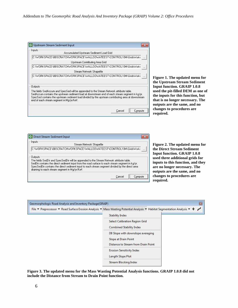
Figure 1. The updated menu for
the Upstream Stream Sediment
Input function. GRAIP 1.0.8
used the pit-filled DEM as one of
the inputs for this function, but
that is no longer necessary. The
outputs are the same, and no
changes to procedures are
required.
Figure 2. The updated menu for
the Direct Stream Sediment
Input function. GRAIP 1.0.8
used three additional grids for
inputs to this function, and they
are no longer necessary. The
outputs are the same, and no
changes to procedures are
required.
Figure 3. The updated menu for the Mass Wasting Potential Analysis functions. GRAIP 1.0.8 did not
include the Distance from Stream to Drain Point function.
Addendum to The Geomorphic Road Analysis And Inventory Package (GRAIP) Volume 2: Office Procedures
7
SECTION II: REPLACEMENT INSTRUCTIONS
The following sections are to be referred to in place of their corresponding
sections in the original manual. The updates made with GRAIP 1.0.9 changed the
information and procedures substantially in these sections.
- Preprocessing Shapefiles, pp. 40-46 in the original manual
- Running TauDEM, pp. 72-76 in the original manual
- Mass Wasting Potential Analysis, pp. 100-117 in the original manual
- Appendix D: Attribute Table Field Name Explanations, DrainPoints Attribute
Table only, pp. 136-137 in the original manual
Preprocessing Shapefiles
This section replaces the Preprocessing Shapefiles section under Section II of the
office manual, pp. 40-46.
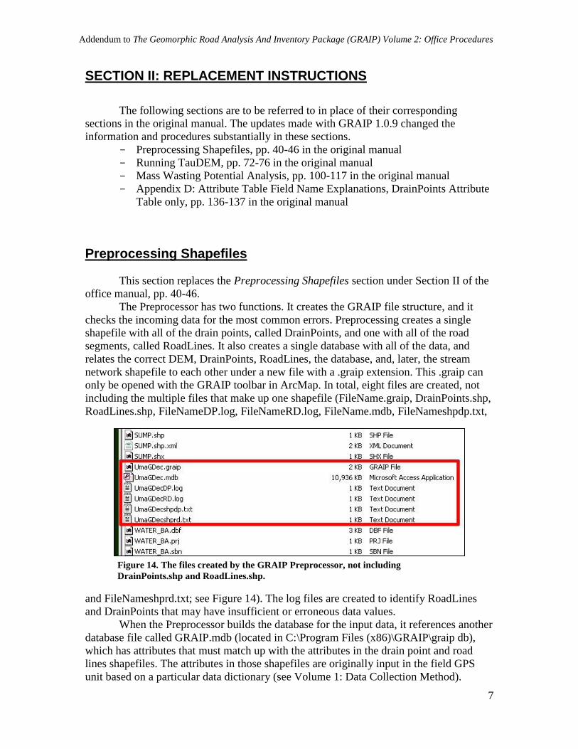
The Preprocessor has two functions. It creates the GRAIP file structure, and it
checks the incoming data for the most common errors. Preprocessing creates a single
shapefile with all of the drain points, called DrainPoints, and one with all of the road
segments, called RoadLines. It also creates a single database with all of the data, and
relates the correct DEM, DrainPoints, RoadLines, the database, and, later, the stream
network shapefile to each other under a new file with a .graip extension. This .graip can
only be opened with the GRAIP toolbar in ArcMap. In total, eight files are created, not
including the multiple files that make up one shapefile (FileName.graip, DrainPoints.shp,
RoadLines.shp, FileNameDP.log, FileNameRD.log, FileName.mdb, FileNameshpdp.txt,
and FileNameshprd.txt; see Figure 14). The log files are created to identify RoadLines
and DrainPoints that may have insufficient or erroneous data values.
When the Preprocessor builds the database for the input data, it references another
database file called GRAIP.mdb (located in C:\Program Files (x86)\GRAIP\graip db),
which has attributes that must match up with the attributes in the drain point and road
lines shapefiles. The attributes in those shapefiles are originally input in the field GPS
unit based on a particular data dictionary (see Volume 1: Data Collection Method).
Figure 14. The files created by the GRAIP Preprocessor, not including
DrainPoints.shp and RoadLines.shp.
Addendum to The Geomorphic Road Analysis And Inventory Package (GRAIP) Volume 2: Office Procedures
8
Essentially, in order for everything to match up correctly at this step, the data dictionary
used for field collection and the GRAIP.mdb file must match. The current data
dictionaries are INVENT5_0 and INVENT5_0_W, and are available on the GRAIP
website (http://www.fs.fed.us/GRAIP/downloads.shtml). Use these when collecting new
data.
GRAIP 1.0.9 has preserved the ability to use the previous version of the field data
dictionary, INVENT4_2. However, the steps to use INVENT4_2 have changed from
GRAIP 1.0.8. Previously, the GRAIP.mdb file would be copied into the working
directory for GRAIP under Program Files on the hard drive. Due to changes in the way
administrative permissions are granted on Forest Service computers, this process has
changed, so that now the GRAIP.mdb file is copied by hand into the workspace in which
you will create the .graip file, and then re-named to match the name you give to the .graip
file. When you do this, make sure to not replace the MDB file when the GRAIP
Preprocessor asks. GRAIP will automatically complete this step if you are using
INVENT5_0 or INVENT5_0_W.
Data collected with INVENT5_0 and INVENT5_0_W are not compatible with
INVENT4_2 data in the model. In other words, you cannot combine old data with new
data in the same GRAIP modeling run.
1. If your data was not collected using the INVENT4_2 data dictionary, skip this step
and proceed to step 2. The GRAIP Preprocessor copies the GRAIP.mdb database
from C:\Program Files (x86)\GRAIP\graip db into the workspace in which you are
creating the .graip file, and renames it as FileName.mdb (where “FileName” is the
name you give your .graip file). The GRAIP.mdb database in Program Files
(x86)\GRAIP\graip db is set up for INVENT5_0 and INVENT5_0_W, so if you have
data in INVENT4_2, you must trick GRAIP into using the GRAIP.mdb file for
INVENT4_2.
a. If you do not have a copy of the INVENT4_2 GRAIP.mdb database, look on the
website or contact us.
b. In Windows (as opposed to Arc Catalog), copy and paste the GRAIP.mdb
database that applies to INVENT4_2 into the workspace where you will create the
.graip file.
c. Rename the GRAIP.mdb database to match the name you will give to your .graip
file.
i. For example, if you are naming your .graip file “sasquatch.graip”, then you
would name your copied MDB database as “sasquatch.mdb”.
2. Open the GRAIP Preprocessor
Addendum to The Geomorphic Road Analysis And Inventory Package (GRAIP) Volume 2: Office Procedures
9
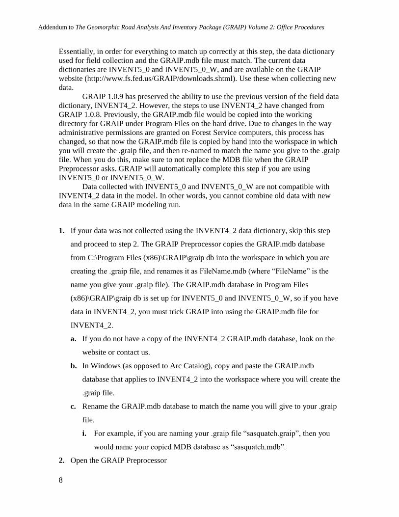
a. This is a separate program, installed with the GRAIP Toolbar and found in the
GRAIP folder under Programs in the Start menu.
3. Create a new .graip file
a. Under Project File, click the {…} button, navigate to the folder with your
shapefiles or wherever you want to save the .graip and other created files.
b. Name the file with something relevant. Do not use spaces. Click OK. FileName is
used here to refer to the .graip, etc.
4. Select the DEM
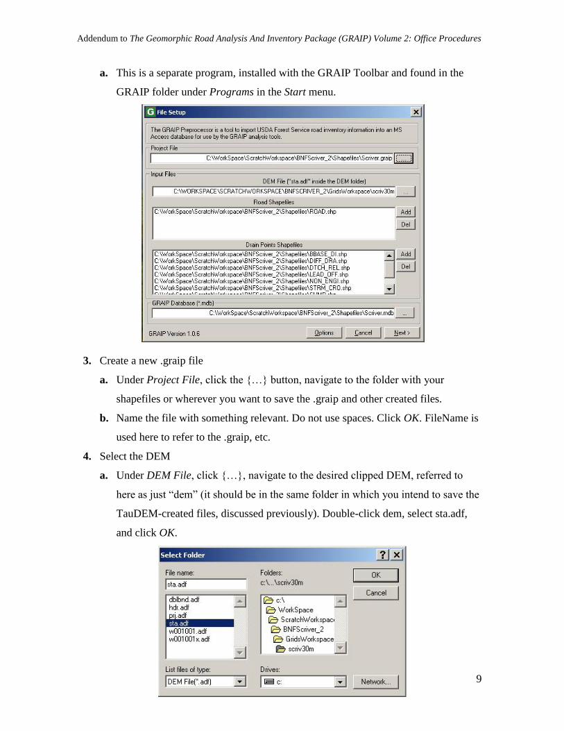
a. Under DEM File, click {…}, navigate to the desired clipped DEM, referred to
here as just “dem” (it should be in the same folder in which you intend to save the
TauDEM-created files, discussed previously). Double-click dem, select sta.adf,
and click OK.
Addendum to The Geomorphic Road Analysis And Inventory Package (GRAIP) Volume 2: Office Procedures
10
b. If you don’t have the DEM, you can still correct errors. For this step, use a
dummy DEM (any DEM). You will have to re-preprocess the data with the
correct DEM before running GRAIP.
5. Add the road shapefile(s), and the drain point shapefiles.
a. Under Road Shapefiles, click Add. Navigate to the location of the ROAD
shapefile(s), select them, and click OK.
b. Under Drain Points Shapefiles, click Add, Navigate to the location of the drain
point shapefiles, select all of the drain point shapefiles, and click OK. There are
nine possible drain point shapefiles, but not every study will have them all. They
are BBASE_DI, DIFF_DRA, DTCH_REL, EXCAV_ST, LEAD_OFF,
NON_ENGI, STRM_CRO, SUMP, and WATER_BA.
c. You can add more than one shapefile with the same name, as if you imported,
corrected, and exported the shapefiles in two batches. In this case, the second (or
even third or fourth) set of shapefiles should be in a separate sub-workspace in the
same workspace as the rest of the shapefiles.
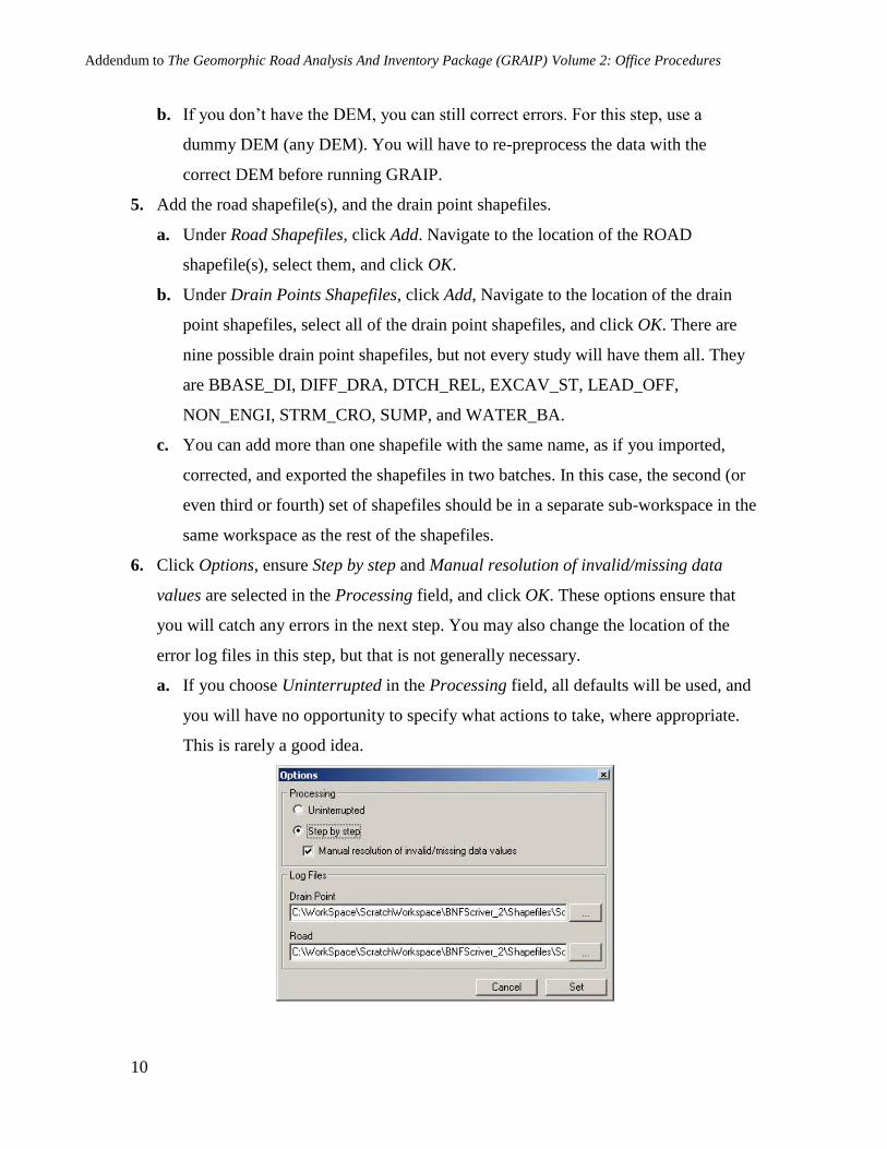
6. Click Options, ensure Step by step and Manual resolution of invalid/missing data
values are selected in the Processing field, and click OK. These options ensure that
you will catch any errors in the next step. You may also change the location of the
error log files in this step, but that is not generally necessary.
a. If you choose Uninterrupted in the Processing field, all defaults will be used, and
you will have no opportunity to specify what actions to take, where appropriate.
This is rarely a good idea.
Addendum to The Geomorphic Road Analysis And Inventory Package (GRAIP) Volume 2: Office Procedures
11
7. Click Next. At this point, all of the files that are created by the preprocessor have been
created, except DrainPoints.shp and RoadLines.shp. The next steps import the drain
points and road shapefiles.
a. If your data was not collected using INVENT4_2, move to step 8 now. If your
data was collected using INVENT4_2, and you have completed step 1 correctly,
then you will see a dialog box pop up that asks if you want to overwrite the
FileName.mdb that you previously copied into the .graip folder. Click No.
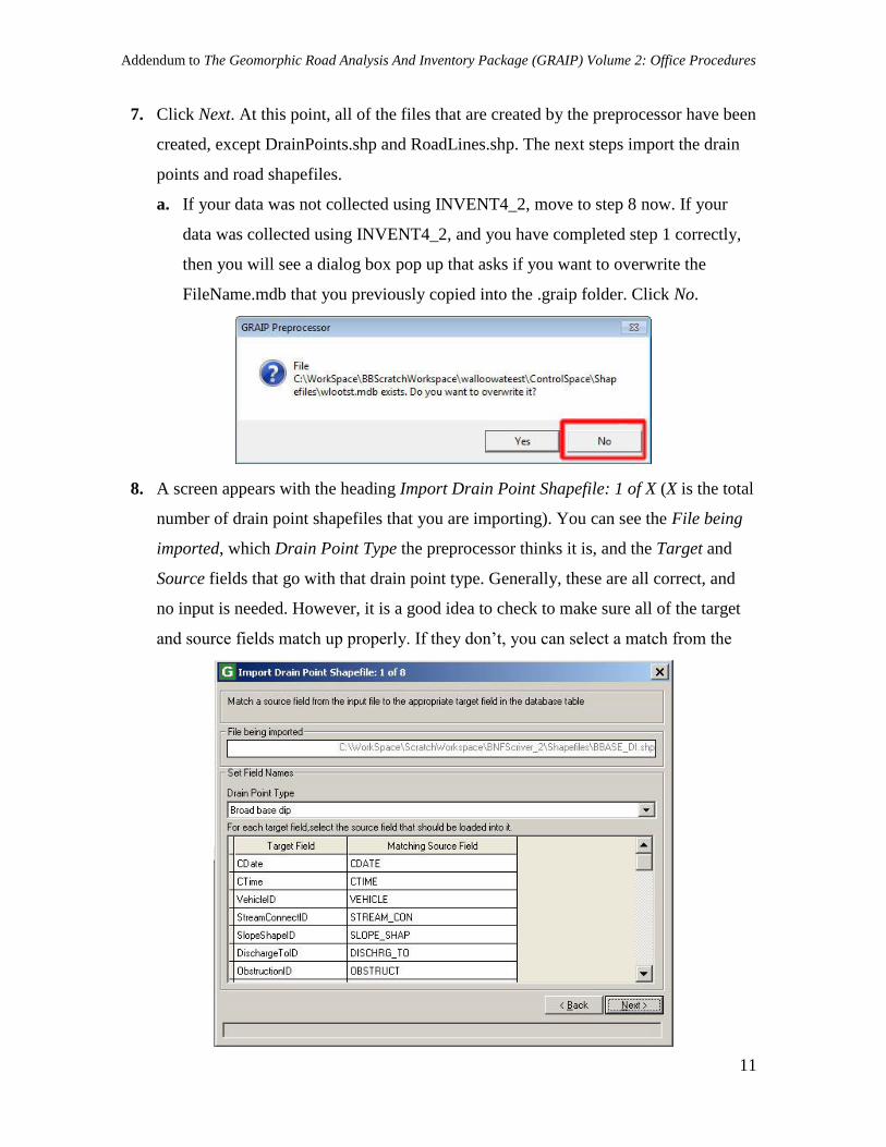
8. A screen appears with the heading Import Drain Point Shapefile: 1 of X (X is the total
number of drain point shapefiles that you are importing). You can see the File being
imported, which Drain Point Type the preprocessor thinks it is, and the Target and
Source fields that go with that drain point type. Generally, these are all correct, and
no input is needed. However, it is a good idea to check to make sure all of the target
and source fields match up properly. If they don’t, you can select a match from the
Addendum to The Geomorphic Road Analysis And Inventory Package (GRAIP) Volume 2: Office Procedures
12
drop-down menu that appears under the Matching Source Field when you click on a
property. If you have the latest version of GRAIP and the latest data dictionary in the
field, this should not occur. If the data dictionary has been modified, the incoming
data may have unexpected values, and the Preprocessor will not be able to
automatically import the data into the GRAIP geodatabase structure. When you are
sure everything matches, click Next. Repeat this process for all drain points and road
lines (the road lines import process is similar).
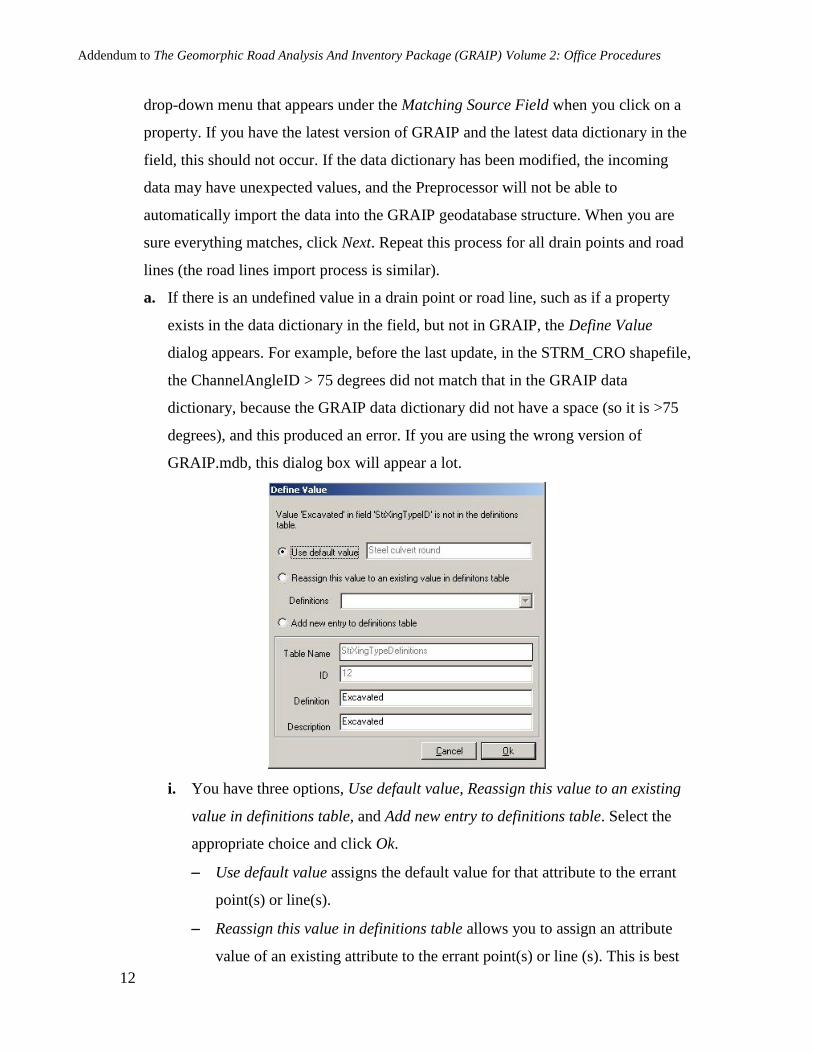
a. If there is an undefined value in a drain point or road line, such as if a property
exists in the data dictionary in the field, but not in GRAIP, the Define Value
dialog appears. For example, before the last update, in the STRM_CRO shapefile,
the ChannelAngleID > 75 degrees did not match that in the GRAIP data
dictionary, because the GRAIP data dictionary did not have a space (so it is >75
degrees), and this produced an error. If you are using the wrong version of
GRAIP.mdb, this dialog box will appear a lot.
i. You have three options, Use default value, Reassign this value to an existing
value in definitions table, and Add new entry to definitions table. Select the
appropriate choice and click Ok.
Use default value assigns the default value for that attribute to the errant
point(s) or line(s).
Reassign this value in definitions table allows you to assign an attribute
value of an existing attribute to the errant point(s) or line (s). This is best
Addendum to The Geomorphic Road Analysis And Inventory Package (GRAIP) Volume 2: Office Procedures
13
to use when there is a misspelled word or similar error, as described
above.
Add new entry to the definitions table adds an entry for the errant value to
the GRAIP MDB definitions table for the .graip. Use this if the value that
is in error is a new value. If this attribute affects a calculation in the
model, the default calculation value will be used.
b. If there are CTime fields in the ROAD shapefile that have anything entered in
them that is not a valid 24-hour time with four digits (e.g. 0745, 0959, 1919, etc.)
or 999, then the Preprocessor will freeze during the Import Road Lines Shapefile
step. Examples of invalid CTime entries include: 9999, 6130, 930, 34, blank cell.
i. If this happens, you must find the errant CTimes and edit them so that they are
valid. Add the ROAD shapefile in which the error occurs to ArcMap, and use
the layer’s attribute table to find and edit the errors. See the instructions for
Editing Data Errors for more information.
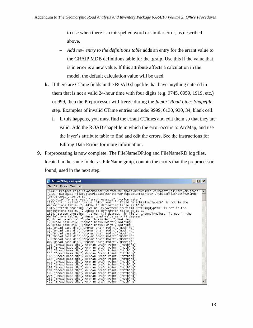
9. Preprocessing is now complete. The FileNameDP.log and FileNameRD.log files,
located in the same folder as FileName.graip, contain the errors that the preprocessor
found, used in the next step.
Addendum to The Geomorphic Road Analysis And Inventory Package (GRAIP) Volume 2: Office Procedures
14
10. In the next step, you will locate and fix any errors. When you re-preprocess the data,
after the errors are corrected, and any time the DEM used does not change (including
if you change which shapefiles are used, so long as the DEM remains the same), you
can just select the already created Project File (FileName.graip) on the first screen,
and click Next. Click OK when asked if you want to delete the DrainPoints,
RoadLines, and FileName.mdb files. Proceed as before. You will have to go through
any Define Value dialogs again. If you change the DEM, you must use a new .graip
(e.g. FileName2.graip). Again, click OK when asked if you want to delete the
DrainPoints, RoadLines, and FileName.mdb files. If no points have been added or
deleted from the original shapefiles, the preprocessor assigns the same
GRAIPDID/GRAIPRID number to each point as it did the first time.
a. If you have data that was collected using INVENT4_2, you will need to delete the
FileName.mdb database, copy a fresh version of the INVENT4_2 GRAIP.mdb
database into the workspace, and rename it as before. Then, when it asks if you
want to delete FileName.mdb, as before, click No. You still want to click Yes
when it asks if you want to delete the DrainPoints and RoadLines files.
Addendum to The Geomorphic Road Analysis And Inventory Package (GRAIP) Volume 2: Office Procedures
15
Running TauDEM
This section replaces the Running TauDEM section under Section III of the office
manual, pp. 72-76.
TauDEM is used to generate a set of grids and shapefiles that are used by GRAIP,
including the stream network shapefile (18 files in total). There are 14 grid files created
by TauDEM (dem stands for the name of the DEM used): demfel, demsd8, demp,
demang, demslp, demad8, demsca, demgord, demplen, demtlen, demsrc, demord, demw,
and demdist. There are two shapefiles created by TauDEM: demnet, demw. The stream
network shapefile (demnet) is associated with FileName.graip, and is added when the
.graip is opened. The last two files are demtree.dat and demcoord.dat. See Appendix F:
TauDEM Inputs and Outputs for more information.
TauDEM may take a long time to run, depending on the size of the DEM (the
maximum grid size is about 7000 x 7000 cells). The folder in which the DEM that is used
is placed will be the folder in which all of the TauDEM-generated files are saved to.
Later, this is the same folder in which SINMAP will create its folder. As such, it is a
good idea to start with a fresh ArcInfo Workspace with only the DEM that you plan to
use in it. TauDEM requires that the DEM name not be any longer than seven characters.
The DEM should be projected to a rectangular coordinate system, such as UTM, rather
than a geographic coordinate system, and should be about 30 m resolution (generally 25-
27 m resolution in the northern two-thirds of the continental U.S.).
1. The projection for the DEM must be defined if it is not already. If it is defined, skip to
step 2.
a. Open ArcMap, add the DEM.
b. Open ArcToolbox.
i. ArcMap Main Menu-> Window-> ArcToolbox, or the button in the Standard
toolbar.
c. In ArcToolbox, go to Data Management-> Projections and Transformations->
Define Projection.
i. Under the Input Dataset or Feature Class, use the drop down menu to select
the DEM.
Addendum to The Geomorphic Road Analysis And Inventory Package (GRAIP) Volume 2: Office Procedures
16
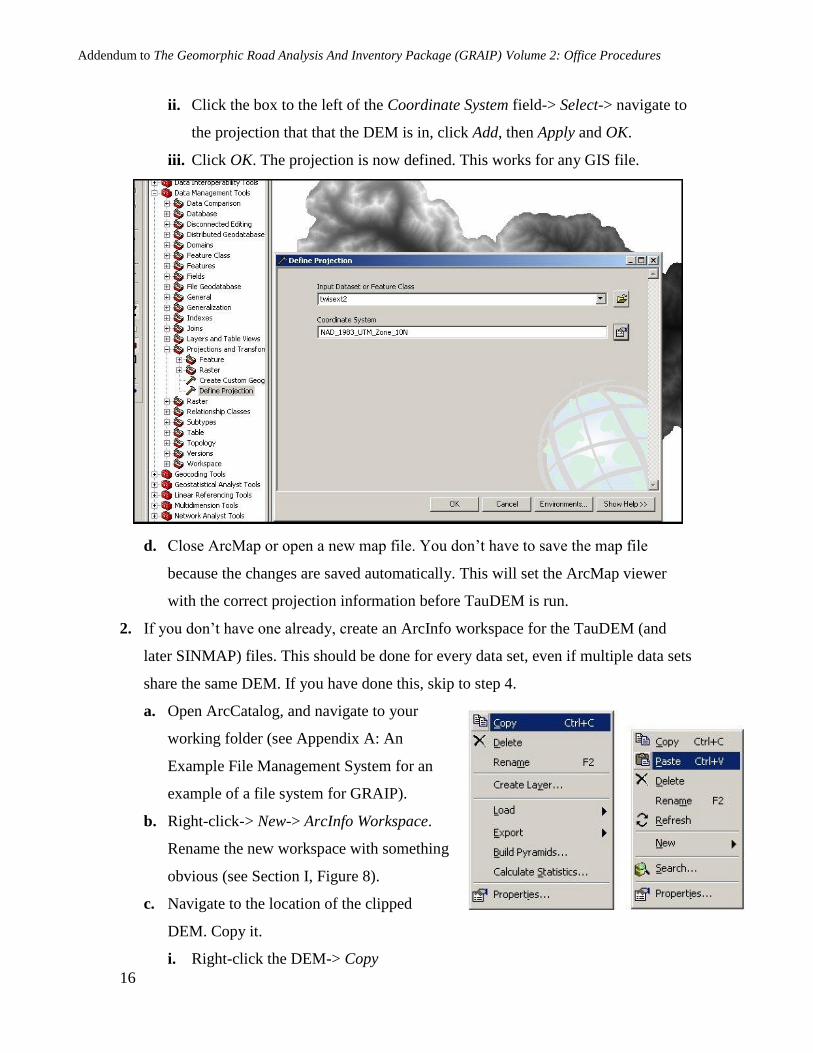
ii. Click the box to the left of the Coordinate System field-> Select-> navigate to
the projection that that the DEM is in, click Add, then Apply and OK.
iii. Click OK. The projection is now defined. This works for any GIS file.
d. Close ArcMap or open a new map file. You don’t have to save the map file
because the changes are saved automatically. This will set the ArcMap viewer
with the correct projection information before TauDEM is run.
2. If you don’t have one already, create an ArcInfo workspace for the TauDEM (and
later SINMAP) files. This should be done for every data set, even if multiple data sets
share the same DEM. If you have done this, skip to step 4.
a. Open ArcCatalog, and navigate to your
working folder (see Appendix A: An
Example File Management System for an
example of a file system for GRAIP).
b. Right-click-> New-> ArcInfo Workspace.
Rename the new workspace with something
obvious (see Section I, Figure 8).
c. Navigate to the location of the clipped
DEM. Copy it.
i. Right-click the DEM-> Copy
Addendum to The Geomorphic Road Analysis And Inventory Package (GRAIP) Volume 2: Office Procedures
17
d. Navigate back to the new workspace and paste the DEM into it.
i. Open the workspace folder.
ii. Right-click anywhere in the folder-> Paste.
e. Close ArcCatalog or navigate away from the new workspace. TauDEM and
ArcGIS might get confused if the workspace they are modifying is active
(currently being viewed) in ArcCatalog at the same time.
3. Open ArcMap and add the clipped DEM with the projection defined from the
TauDEM workspace to the viewer.
4. It is best to do the rest of these steps one immediately after another. From the
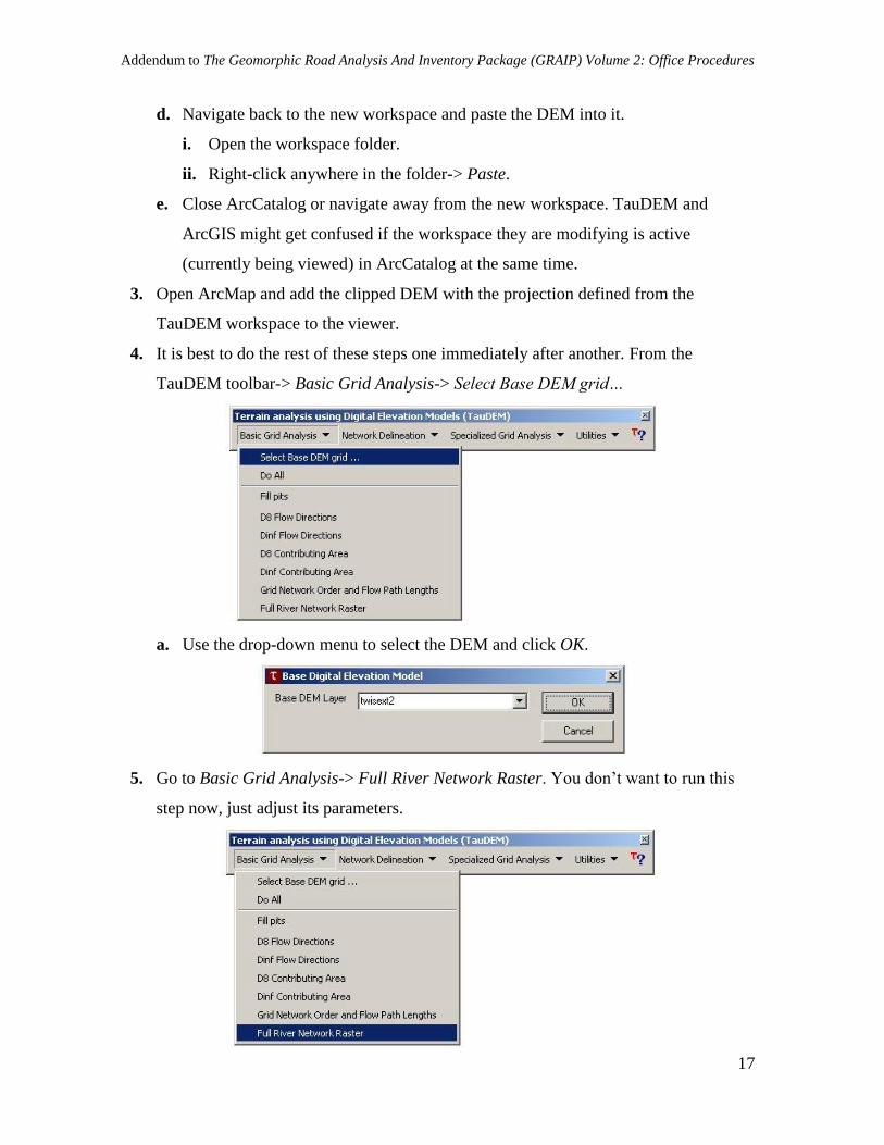
TauDEM toolbar-> Basic Grid Analysis-> Select Base DEM grid…
a. Use the drop-down menu to select the DEM and click OK.
5. Go to Basic Grid Analysis-> Full River Network Raster. You don’t want to run this
step now, just adjust its parameters.
Addendum to The Geomorphic Road Analysis And Inventory Package (GRAIP) Volume 2: Office Procedures
18
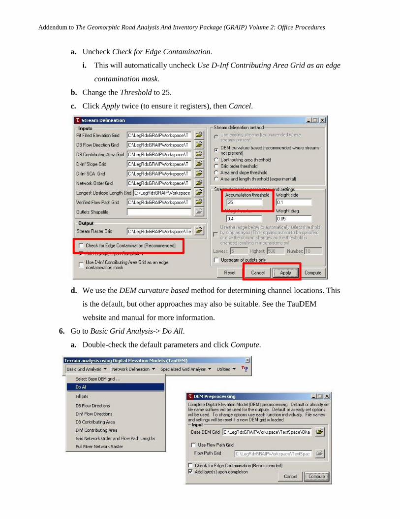
a. Uncheck Check for Edge Contamination.
i. This will automatically uncheck Use D-Inf Contributing Area Grid as an edge
contamination mask.
b. Change the Threshold to 25.
c. Click Apply twice (to ensure it registers), then Cancel.
d. We use the DEM curvature based method for determining channel locations. This
is the default, but other approaches may also be suitable. See the TauDEM
website and manual for more information.
6. Go to Basic Grid Analysis-> Do All.
a. Double-check the default parameters and click Compute.
Addendum to The Geomorphic Road Analysis And Inventory Package (GRAIP) Volume 2: Office Procedures
19
b. This step produces 11 grids (demfel, demsd8, demp, demang, demslp, demad8,
demsca, demgord, demplen, demlen, demsrc).
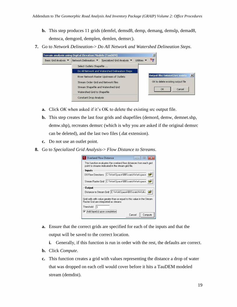
7. Go to Network Delineation-> Do All Network and Watershed Delineation Steps.
a. Click OK when asked if it’s OK to delete the existing src output file.
b. This step creates the last four grids and shapefiles (demord, demw, demnet.shp,
demw.shp), recreates demsrc (which is why you are asked if the original demsrc
can be deleted), and the last two files (.dat extension).
c. Do not use an outlet point.
8. Go to Specialized Grid Analysis-> Flow Distance to Streams.
a. Ensure that the correct grids are specified for each of the inputs and that the
output will be saved to the correct location.
i. Generally, if this function is run in order with the rest, the defaults are correct.
b. Click Compute.
c. This function creates a grid with values representing the distance a drop of water
that was dropped on each cell would cover before it hits a TauDEM modeled
stream (demdist).

Addendum to The Geomorphic Road Analysis And Inventory Package (GRAIP) Volume 2: Office Procedures
20
9. Before proceeding, close ArcMap or open a new map file. This will allow for a fresh
start for the next section. You don’t have to save the map file because grids and
shapefiles are already saved on the hard drive.
Addendum to The Geomorphic Road Analysis And Inventory Package (GRAIP) Volume 2: Office Procedures
21
Mass Wasting Potential Analysis
This section replaces the Mass Wasting Potential Analysis section under Section
III of the office manual, pp. 99-117.
The functions in the Mass Wasting Potential Analysis menu produce data that
indicate the likelihood of mass wasting events caused by concentrated road drainage
discharging onto the hillslope below a road. The default parameters can often be adjusted
to provide more accurate results. The risk predictions can be compared to the data
produced by SINMAP for a road vs. no road comparison.
There are nine tools under the Mass Wasting Potential Analysis menu heading.
These steps can be undertaken only after SINMAP has been run. The first step finds the
stability index at each drain point from the demsi grid that SINMAP created, and
populates the SI column in the DrainPoints table. The second and third tools create the
combined stability index grid and four other intermediary grids (demsic, demrmin,
demrmax, demrdmin, and demrdmax, respectively), and one text file (demcalp.csv) that
take the road water into account for landslide risk. The SIR column is also populated in
the DrainPoints table. The combined stability index grid (demsic) can be compared to the
stability index grid (demsi, from above) to see the affect the road has on the terrain
stability.
The fourth and fifth steps create a slope grid (demslpd) and populate the Slope
column of the DrainPoints table, which is the slope of the hillslope below each drain
point. The sixth step uses the demdist grid created by TauDEM to populate the
DistToStre column in the DrainPoints table. The next step addresses gully initiation risk
with the Erosion Sensitivity Index, and so populates the ESI column of the DrainPoints
table. The eighth step creates a road length vs. hillslope plot called L-S Plot (note that the
Y-axis is logarithmic) that can be used to calibrate the ESI threshold for increased gully
risk (ESIcrit). The final step calculates the Stream Blocking Index (SBI) for each stream
crossing, and so populates the PipeDiaToChanWidthRatio, PipeDiaToChanWidthScore,
SkewAngle, SkewAngleScore, and SBI columns in the DrainPoints table.
The combined stability index grid adds water from the road at each drain point to
the hillslope, based on the contributing length of road and a predetermined additional
road runoff rate (effectively increasing the contributing area at the cells in which the
drain points lie). The overall effect is to decrease slope stability at the location of each
drain point that receives road water. Slope stability will not increase from possible
interception of shallow groundwater by a ditch, as GRAIP only accounts for the added
surface runoff.
1. If not already open, open ArcMap or a new map window and open the GRAIP file
(the .graip).
Addendum to The Geomorphic Road Analysis And Inventory Package (GRAIP) Volume 2: Office Procedures
22
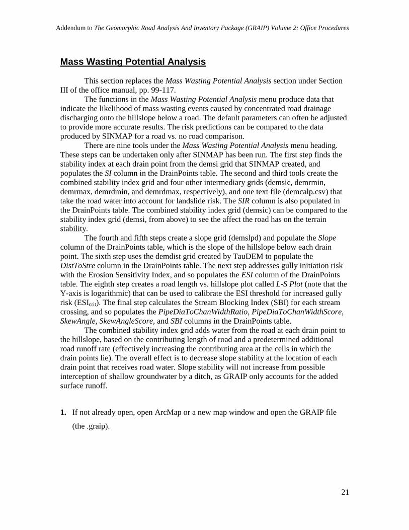
2. GRAIP toolbar-> Mass Wasting Potential Analysis-> Stability Index
a. Ensure that the DrainPoints shapefile and each of the grids are correctly located,
and click Compute.
b. Check that the SI column has been populated in the DrainPoints Attribute Table.
There should not be any zero values.
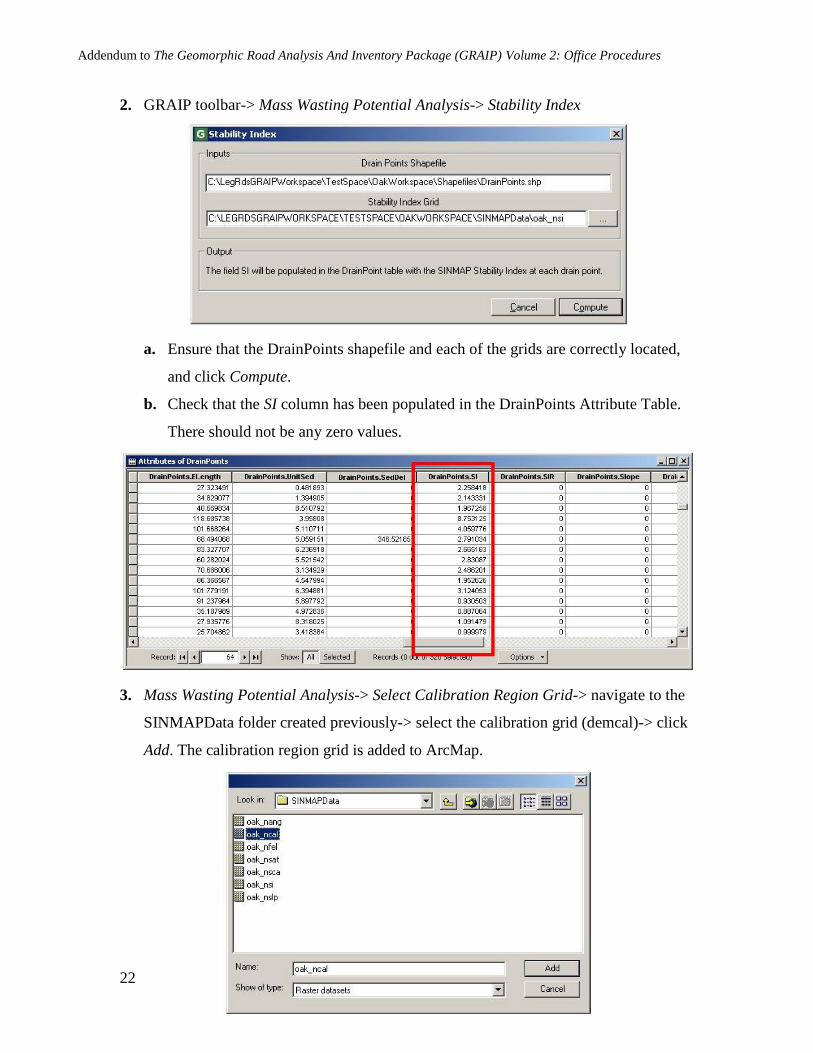
3. Mass Wasting Potential Analysis-> Select Calibration Region Grid-> navigate to the
SINMAPData folder created previously-> select the calibration grid (demcal)-> click
Add. The calibration region grid is added to ArcMap.
Addendum to The Geomorphic Road Analysis And Inventory Package (GRAIP) Volume 2: Office Procedures
23
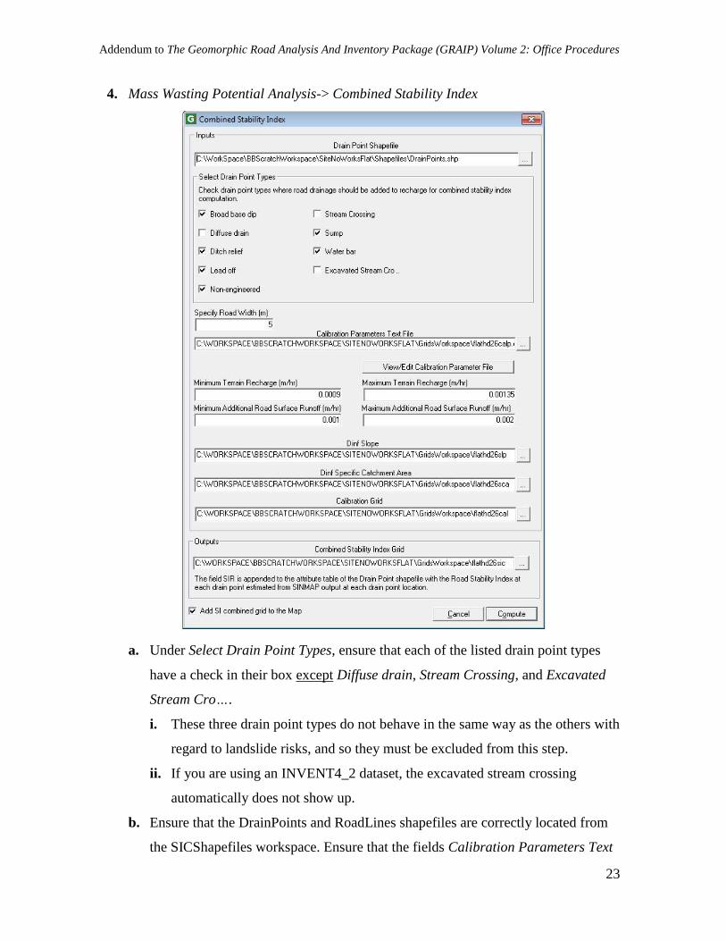
4. Mass Wasting Potential Analysis-> Combined Stability Index
a. Under Select Drain Point Types, ensure that each of the listed drain point types
have a check in their box except Diffuse drain, Stream Crossing, and Excavated
Stream Cro….
i. These three drain point types do not behave in the same way as the others with
regard to landslide risks, and so they must be excluded from this step.
ii. If you are using an INVENT4_2 dataset, the excavated stream crossing
automatically does not show up.
b. Ensure that the DrainPoints and RoadLines shapefiles are correctly located from
the SICShapefiles workspace. Ensure that the fields Calibration Parameters Text
Addendum to The Geomorphic Road Analysis And Inventory Package (GRAIP) Volume 2: Office Procedures
24
File, Dinf Slope, Dinf Specific Catchment Area, and Calibration Grid are
correctly populated and located (demcalp.csv, demslp, and demsca from the
TauDEM folder, and demcal from the SINMAPData folder, respectively).
c. The following are default parameters:
i. Specify Road Width (m) is 5.
ii. Minimum Terrain Recharge (m/hr) is 0.0009.
iii. Maximum Terrain Recharge (m/hr) is 0.00135.
iv. Minimum Additional Road Surface Runoff (m/hr) is 0.001.
v. Maximum Additional Road Surface Runoff (m/hr) is 0.002.
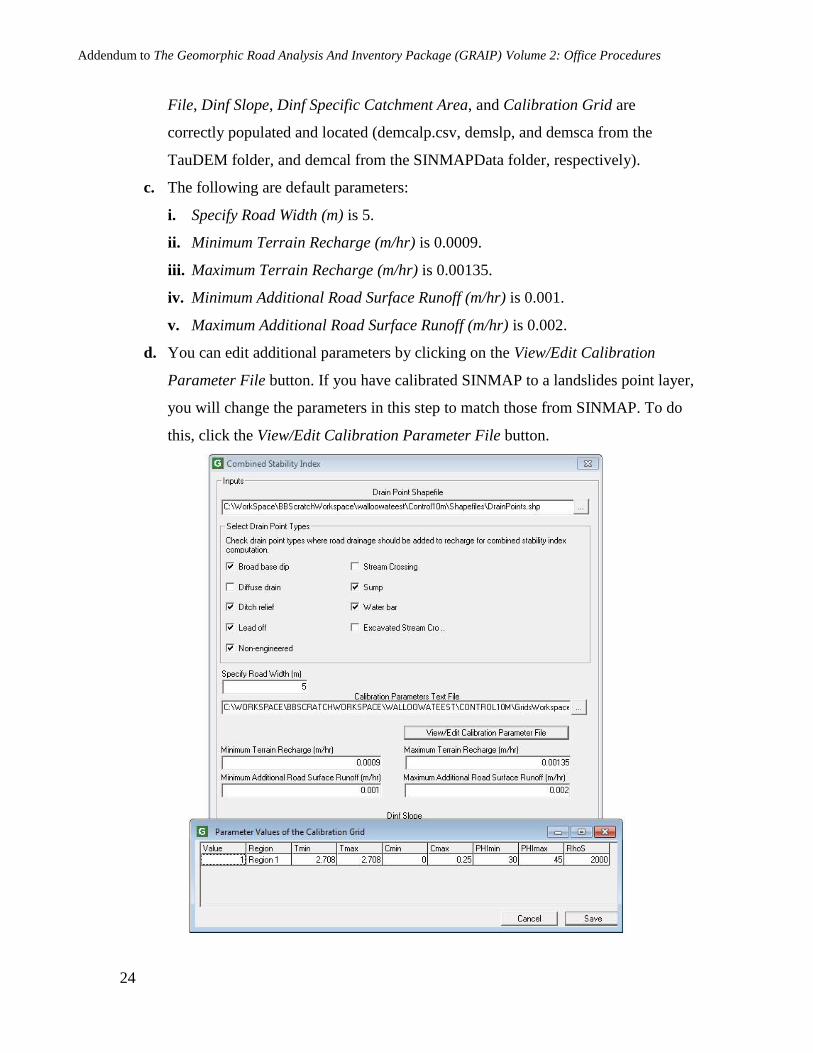
d. You can edit additional parameters by clicking on the View/Edit Calibration
Parameter File button. If you have calibrated SINMAP to a landslides point layer,
you will change the parameters in this step to match those from SINMAP. To do
this, click the View/Edit Calibration Parameter File button.
Addendum to The Geomorphic Road Analysis And Inventory Package (GRAIP) Volume 2: Office Procedures
25
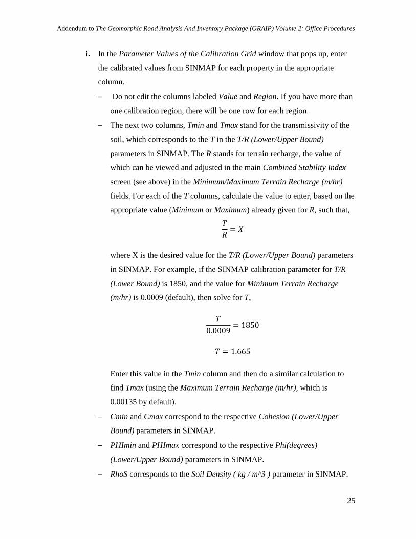
i. In the Parameter Values of the Calibration Grid window that pops up, enter
the calibrated values from SINMAP for each property in the appropriate
column.
Do not edit the columns labeled Value and Region. If you have more than
one calibration region, there will be one row for each region.
The next two columns, Tmin and Tmax stand for the transmissivity of the
soil, which corresponds to the T in the T/R (Lower/Upper Bound)
parameters in SINMAP. The R stands for terrain recharge, the value of
which can be viewed and adjusted in the main Combined Stability Index
screen (see above) in the Minimum/Maximum Terrain Recharge (m/hr)
fields. For each of the T columns, calculate the value to enter, based on the
appropriate value (Minimum or Maximum) already given for R, such that,
where X is the desired value for the T/R (Lower/Upper Bound) parameters
in SINMAP. For example, if the SINMAP calibration parameter for T/R
(Lower Bound) is 1850, and the value for Minimum Terrain Recharge
(m/hr) is 0.0009 (default), then solve for T,
Enter this value in the Tmin column and then do a similar calculation to
find Tmax (using the Maximum Terrain Recharge (m/hr), which is
0.00135 by default).
Cmin and Cmax correspond to the respective Cohesion (Lower/Upper
Bound) parameters in SINMAP.
PHImin and PHImax correspond to the respective Phi(degrees)
(Lower/Upper Bound) parameters in SINMAP.
RhoS corresponds to the Soil Density ( kg / m^3 ) parameter in SINMAP.
Addendum to The Geomorphic Road Analysis And Inventory Package (GRAIP) Volume 2: Office Procedures
26
ii. Click Save. The previously defined (in SINMAP) calibration parameters will
be used to generate the Combined Stability Index grid.
e. Ensure that the Combined Stability Index Grid will be saved to the correct place.
Do not change its name.
f. Check Add SI combined grid to map and click Compute.
g. Five grids and one text file (calibration parameters; demcalp.csv) are created:
i. The combined stability index grid (demsic) is added to ArcMap and saved
wherever you specified.
ii. The minimum and maximum depth of terrain runoff grids (demrmin and
demrmax) are not added to ArcMap and are saved to the same place as the
TauDEM files. These files are intermediary (i.e. they are used by the
Combined Stability Index function and nothing else)
iii. The specific discharge due to minimum and maximum runoff grids
(demrdmin and demrdmax) are not added to ArcMap. These files are
intermediary.
h. Sometimes, GRAIP and SINMAP may round certain values slightly differently,
which results in an SI grid (demsi) that does not match up perfectly with the SIC
(demsic), even where there are no roads. You may want to use the Combined
Stability Index function to create a matching SI grid. To do this, run this function
again, setting both the Minimum Additional Road Surface Runoff (m/hr) and
Maximum Additional Road Surface Runoff (m/hr) to 0. This removes the road
water from the equation, resulting in an equivalent to the SI grid.
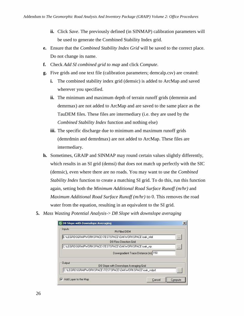
5. Mass Wasting Potential Analysis-> D8 Slope with downslope averaging
Addendum to The Geomorphic Road Analysis And Inventory Package (GRAIP) Volume 2: Office Procedures
27
a. The purpose of this function is to generate a grid of slopes at each cell that will be
used to determine the slope at each drain point, which is used to help determine
the Erosion Sensitivity Index (see below). The method used estimates the slope at
each cell by averaging the slope from that cell to a cell that is located a specified
trace distance downhill.
b. Ensure that the Pit Filled DEM (demfel) and D8 Flow Direction Grid (demp) are
correctly located.
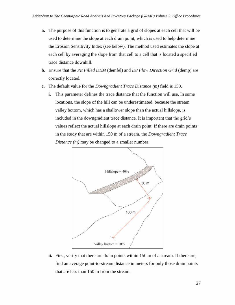
c. The default value for the Downgradient Trace Distance (m) field is 150.
i. This parameter defines the trace distance that the function will use. In some
locations, the slope of the hill can be underestimated, because the stream
valley bottom, which has a shallower slope than the actual hillslope, is
included in the downgradient trace distance. It is important that the grid’s
values reflect the actual hillslope at each drain point. If there are drain points
in the study that are within 150 m of a stream, the Downgradient Trace
Distance (m) may be changed to a smaller number.
ii. First, verify that there are drain points within 150 m of a stream. If there are,
find an average point-to-stream distance in meters for only those drain points
that are less than 150 m from the stream.
Addendum to The Geomorphic Road Analysis And Inventory Package (GRAIP) Volume 2: Office Procedures
28
iii. Since the DEM has a resolution of about 30 m, and you need two grid cell
values to determine slope, you need an absolute minimum of 45 m of
downslope trace distance (the length of the diagonal across a 30 m square is
about 42 m). The simplest way to determine what the Downgradient Trace
Distance should be is to take the greater of either the average point-to-stream
distance or 45 m. However, the longer the specified trace distance, the more
accurate the average (assuming a relatively constant slope on the hillslope). A
slope calculated using only two grid cells will probably not be very accurate,
due to imprecision in the 30 m DEM grid values. While 45 m might be a good
distance to use for those points which are very close to the stream, it will not
produce accurate results for points further away.
It is highly recommended that you use a number higher than 90 m. This
would include three grid cells at a diagonal.
If most of the drain points that are within 150 m of the stream are within
the same grid cell as the stream, then there is no way to take an accurate
average hillslope, anyway, so these point-to-stream distances should be
removed from consideration.
If there is only a small percentage of points within 150 m of the stream,
then you may also consider using the default 150 m. This will result in
inaccurate slope values for those points within 150 m, but the majority of
points will have more accurate values.
d. Ensure that the D8 Slope with Downslope Averaging Grid will be saved to the
correct place. Do not change the name.
e. Click Compute. The layer will be added to the map, but can be turned off to save
drawing time.
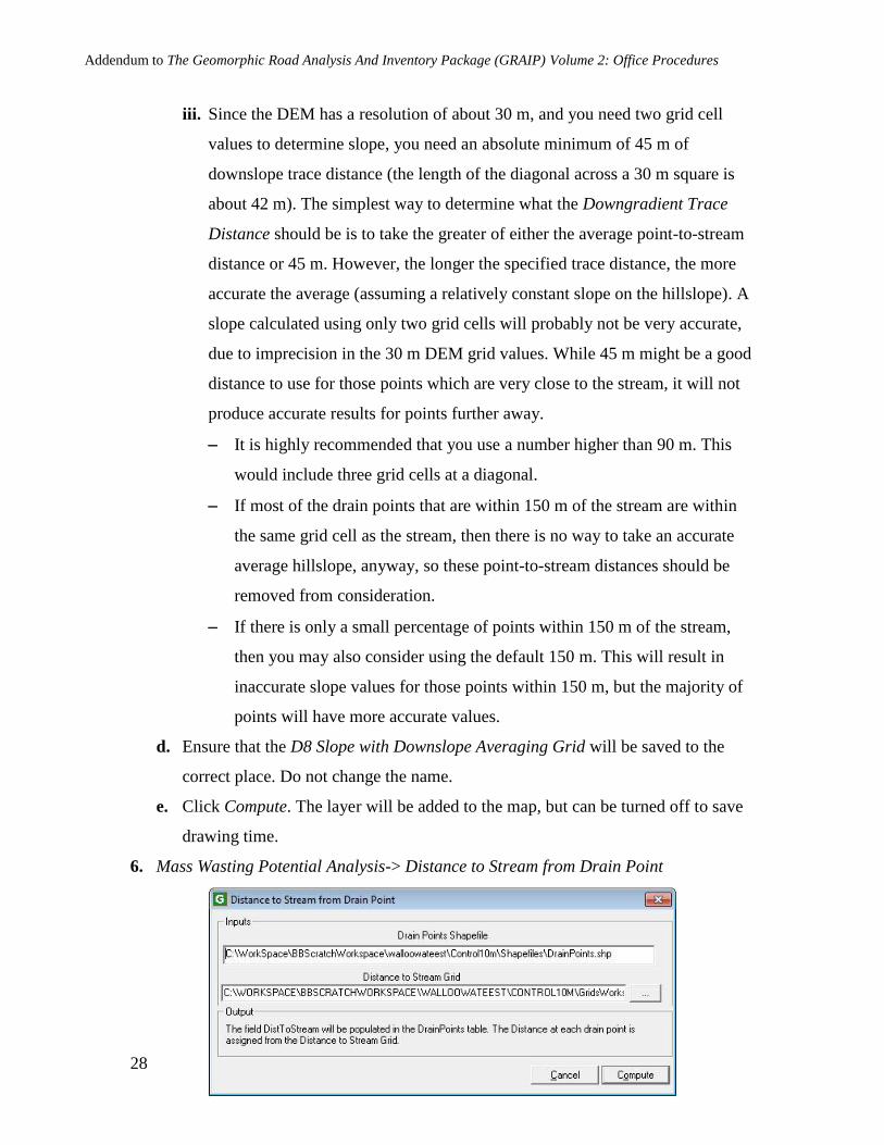
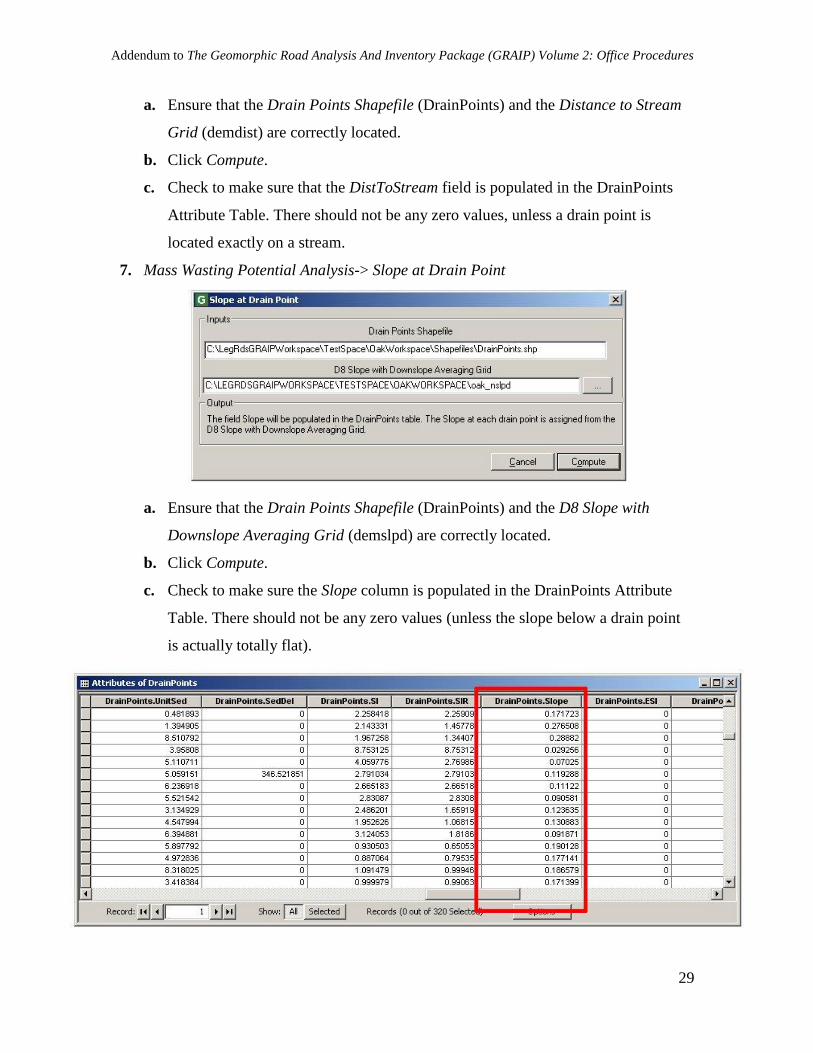
6. Mass Wasting Potential Analysis-> Distance to Stream from Drain Point
Addendum to The Geomorphic Road Analysis And Inventory Package (GRAIP) Volume 2: Office Procedures
29
a. Ensure that the Drain Points Shapefile (DrainPoints) and the Distance to Stream
Grid (demdist) are correctly located.
b. Click Compute.
c. Check to make sure that the DistToStream field is populated in the DrainPoints
Attribute Table. There should not be any zero values, unless a drain point is
located exactly on a stream.
7. Mass Wasting Potential Analysis-> Slope at Drain Point
a. Ensure that the Drain Points Shapefile (DrainPoints) and the D8 Slope with
Downslope Averaging Grid (demslpd) are correctly located.
b. Click Compute.
c. Check to make sure the Slope column is populated in the DrainPoints Attribute
Table. There should not be any zero values (unless the slope below a drain point
is actually totally flat).
Addendum to The Geomorphic Road Analysis And Inventory Package (GRAIP) Volume 2: Office Procedures
30
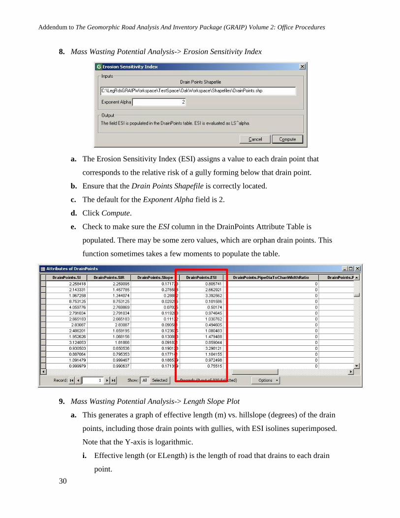
8. Mass Wasting Potential Analysis-> Erosion Sensitivity Index
a. The Erosion Sensitivity Index (ESI) assigns a value to each drain point that
corresponds to the relative risk of a gully forming below that drain point.
b. Ensure that the Drain Points Shapefile is correctly located.
c. The default for the Exponent Alpha field is 2.
d. Click Compute.
e. Check to make sure the ESI column in the DrainPoints Attribute Table is
populated. There may be some zero values, which are orphan drain points. This
function sometimes takes a few moments to populate the table.
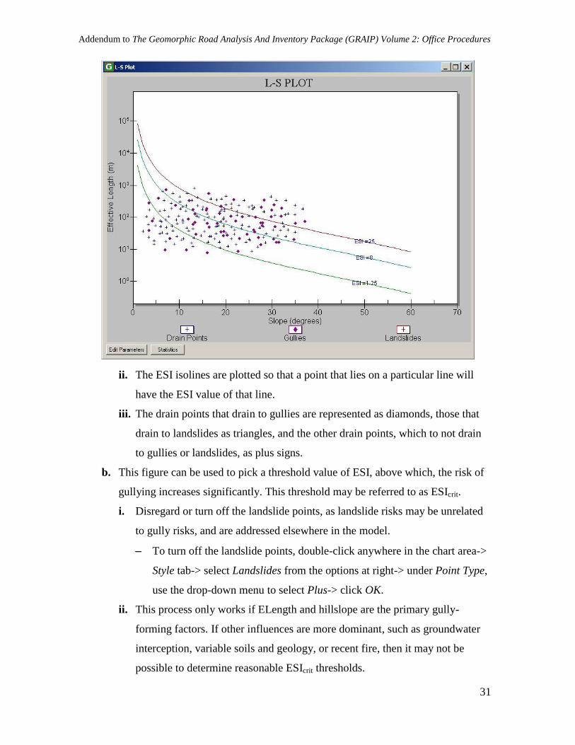
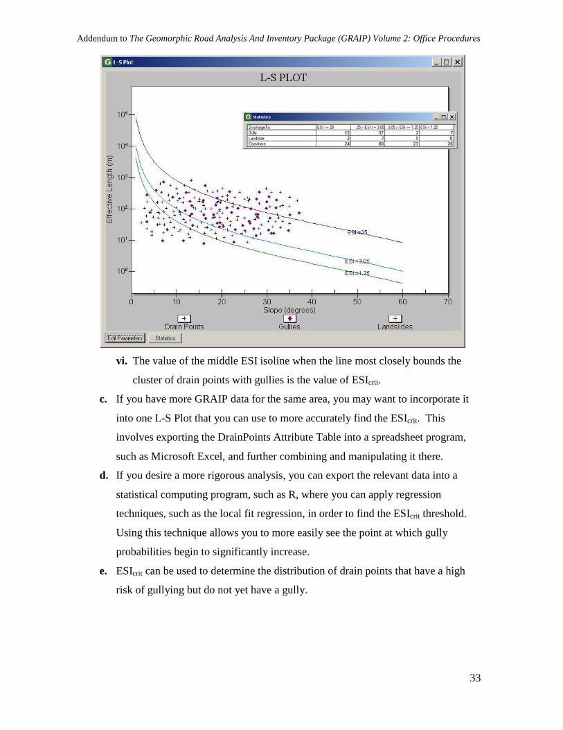
9. Mass Wasting Potential Analysis-> Length Slope Plot
a. This generates a graph of effective length (m) vs. hillslope (degrees) of the drain
points, including those drain points with gullies, with ESI isolines superimposed.
Note that the Y-axis is logarithmic.
i. Effective length (or ELength) is the length of road that drains to each drain
point.
Addendum to The Geomorphic Road Analysis And Inventory Package (GRAIP) Volume 2: Office Procedures
31
ii. The ESI isolines are plotted so that a point that lies on a particular line will
have the ESI value of that line.
iii. The drain points that drain to gullies are represented as diamonds, those that
drain to landslides as triangles, and the other drain points, which to not drain
to gullies or landslides, as plus signs.
b. This figure can be used to pick a threshold value of ESI, above which, the risk of
gullying increases significantly. This threshold may be referred to as ESIcrit.
i. Disregard or turn off the landslide points, as landslide risks may be unrelated
to gully risks, and are addressed elsewhere in the model.
To turn off the landslide points, double-click anywhere in the chart area->
Style tab-> select Landslides from the options at right-> under Point Type,
use the drop-down menu to select Plus-> click OK.
ii. This process only works if ELength and hillslope are the primary gully-
forming factors. If other influences are more dominant, such as groundwater
interception, variable soils and geology, or recent fire, then it may not be
possible to determine reasonable ESIcrit thresholds.
Addendum to The Geomorphic Road Analysis And Inventory Package (GRAIP) Volume 2: Office Procedures
32
iii. Generally, if there are not many gullies observed at drain points in your area,
then gullying may not be of enough concern to complete this calibration
process. For example, if you have a watershed with 5000 drain points, and
only 25 of them have small gullies (0.5%), then the risks of further gully
forming are probably not very high. However, if you have only 100 drain
points, and only 5 gullies (5%), then sufficient risk probably exists to justify
this calibration process. Note that, assuming your gullies fit the ELength-
hillslope model, the more gullies you have, the easier and more accurate your
calibration will be.
iv. Notice that the distribution of drain points with gullies is weighted to the
regions of the graph with higher ESI (further right and up; longer ELength and
steeper slope). Therefore, the higher the ESI of a drain point, the higher the
risk of gullying.
If this distribution trend is not present, then it is likely that the gullies
recorded in your data have other contributors. If this is the case, you may
have success if you can determine which points are affected by external
factors and remove them from consideration.
v. The goal is to find the ESI isoline that most closely bounds the lower part of
the cluster of drain points with gullies. This process is similar to the process
used in the calibration of SINMAP. You will move the middle ESI isoline
(default value of 8) until you are satisfied with its location.
In the L-S Plot window, click Edit Parameters. From here, you can change
the value of each ESI isoline, as well as the value of alpha (which you first
encountered above in the Erosion Sensitivity Index function; generally,
there is no need to change this value).
Change the value of the Medium ESI field to change the location of the
middle ESI isoline. Larger values move the line up and right; smaller
values move it down and left. Press Ok.
You can view information about the distribution of drain points with
gullies among the ESI regions (i.e. the area between the ESI isolines) by
clicking the Statistics button in the L-S Plot window.
Addendum to The Geomorphic Road Analysis And Inventory Package (GRAIP) Volume 2: Office Procedures
33
vi. The value of the middle ESI isoline when the line most closely bounds the
cluster of drain points with gullies is the value of ESIcrit.
c. If you have more GRAIP data for the same area, you may want to incorporate it
into one L-S Plot that you can use to more accurately find the ESIcrit. This
involves exporting the DrainPoints Attribute Table into a spreadsheet program,
such as Microsoft Excel, and further combining and manipulating it there.
d. If you desire a more rigorous analysis, you can export the relevant data into a
statistical computing program, such as R, where you can apply regression
techniques, such as the local fit regression, in order to find the ESIcrit threshold.
Using this technique allows you to more easily see the point at which gully
probabilities begin to significantly increase.
e. ESIcrit can be used to determine the distribution of drain points that have a high
risk of gullying but do not yet have a gully.
Addendum to The Geomorphic Road Analysis And Inventory Package (GRAIP) Volume 2: Office Procedures
34
f. Nothing is added to any table, created, or saved in this step.
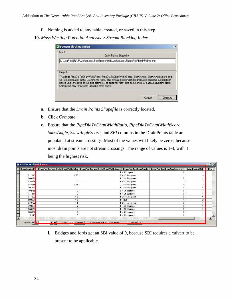
10. Mass Wasting Potential Analysis-> Stream Blocking Index
a. Ensure that the Drain Points Shapefile is correctly located.
b. Click Compute.
c. Ensure that the PipeDiaToChanWidthRatio, PipeDiaToChanWidthScore,
SkewAngle, SkewAngleScore, and SBI columns in the DrainPoints table are
populated at stream crossings. Most of the values will likely be zeros, because
most drain points are not stream crossings. The range of values is 1-4, with 4
being the highest risk.
i. Bridges and fords get an SBI value of 0, because SBI requires a culvert to be
present to be applicable.
Addendum to The Geomorphic Road Analysis And Inventory Package (GRAIP) Volume 2: Office Procedures
35
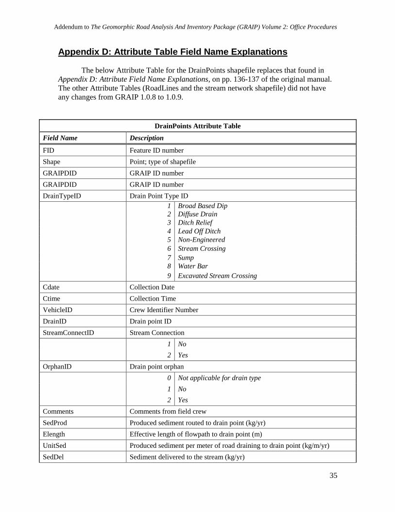
Appendix D: Attribute Table Field Name Explanations
The below Attribute Table for the DrainPoints shapefile replaces that found in
Appendix D: Attribute Field Name Explanations, on pp. 136-137 of the original manual.
The other Attribute Tables (RoadLines and the stream network shapefile) did not have
any changes from GRAIP 1.0.8 to 1.0.9.
DrainPoints Attribute Table
Field Name Description
FID Feature ID number
Shape Point; type of shapefile
GRAIPDID GRAIP ID number
GRAIPDID GRAIP ID number
DrainTypeID Drain Point Type ID
1 Broad Based Dip
2 Diffuse Drain
3 Ditch Relief
4 Lead Off Ditch
5 Non-Engineered
6 Stream Crossing
7 Sump
8 Water Bar
9 Excavated Stream Crossing
Cdate Collection Date
Ctime Collection Time
VehicleID Crew Identifier Number
DrainID Drain point ID
StreamConnectID Stream Connection
1 No
2 Yes
OrphanID Drain point orphan
0 Not applicable for drain type
1 No
2 Yes
Comments Comments from field crew
SedProd Produced sediment routed to drain point (kg/yr)
Elength Effective length of flowpath to drain point (m)
UnitSed Produced sediment per meter of road draining to drain point (kg/m/yr)
SedDel Sediment delivered to the stream (kg/yr)
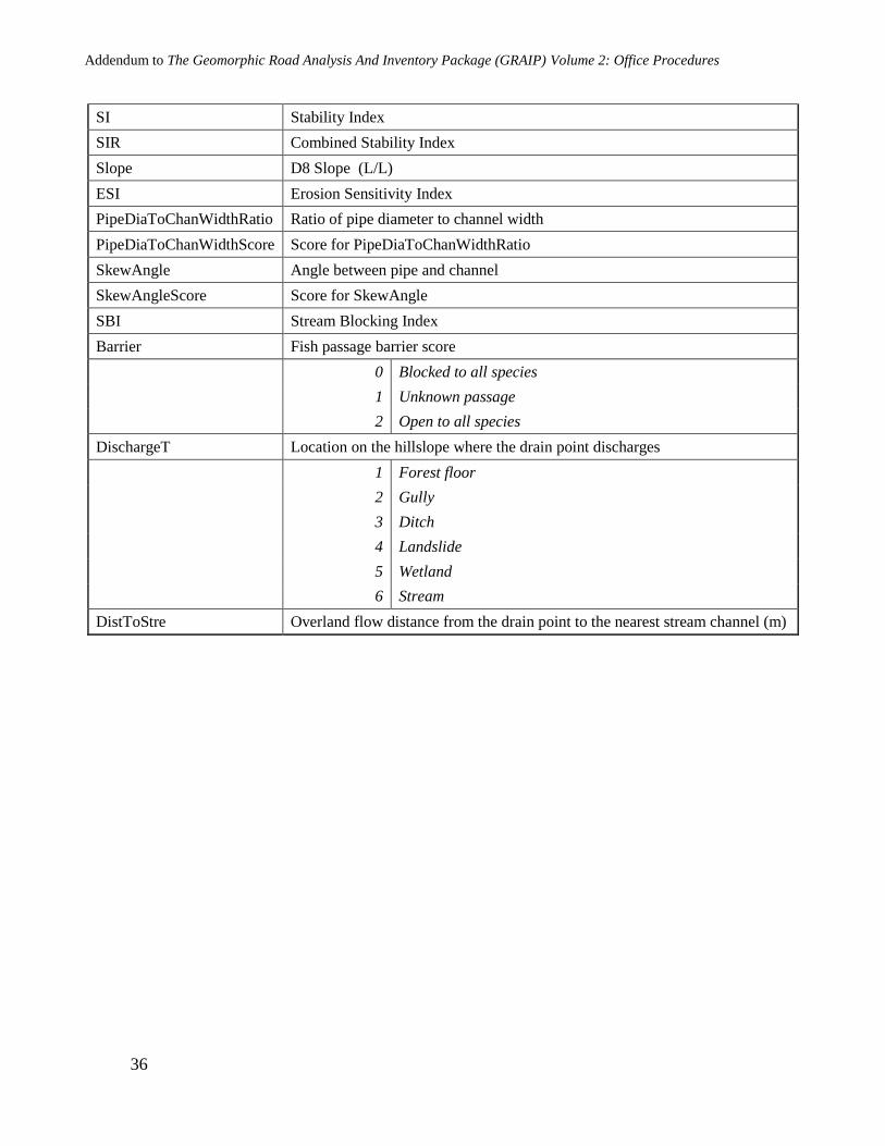
Addendum to The Geomorphic Road Analysis And Inventory Package (GRAIP) Volume 2: Office Procedures
36
SI Stability Index
SIR Combined Stability Index
Slope D8 Slope (L/L)
ESI Erosion Sensitivity Index
PipeDiaToChanWidthRatio Ratio of pipe diameter to channel width
PipeDiaToChanWidthScore Score for PipeDiaToChanWidthRatio
SkewAngle Angle between pipe and channel
SkewAngleScore Score for SkewAngle
SBI Stream Blocking Index
Barrier Fish passage barrier score
0 Blocked to all species
1 Unknown passage
2 Open to all species
DischargeT Location on the hillslope where the drain point discharges
1 Forest floor
2 Gully
3 Ditch
4 Landslide
5 Wetland
6 Stream
DistToStre Overland flow distance from the drain point to the nearest stream channel (m)
Addendum to The Geomorphic Road Analysis And Inventory Package (GRAIP) Volume 2: Office Procedures
37
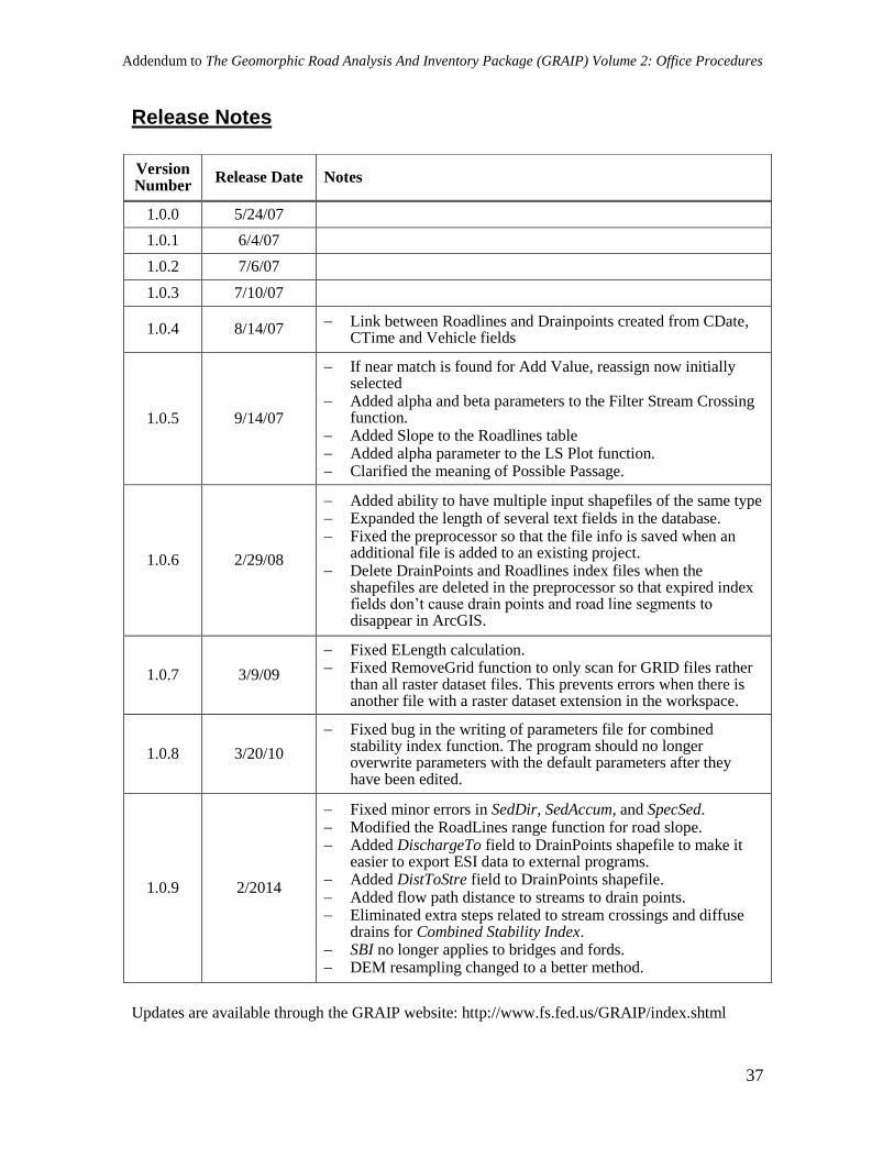
Release Notes
Updates are available through the GRAIP website: http://www.fs.fed.us/GRAIP/index.shtml
Version Number
Release Date Notes
1.0.0 5/24/07
1.0.1 6/4/07
1.0.2 7/6/07
1.0.3 7/10/07
1.0.4 8/14/07 Link between Roadlines and Drainpoints created from CDate,
CTime and Vehicle fields
1.0.5 9/14/07
If near match is found for Add Value, reassign now initially selected
Added alpha and beta parameters to the Filter Stream Crossing function.
Added Slope to the Roadlines table Added alpha parameter to the LS Plot function. Clarified the meaning of Possible Passage.
1.0.6 2/29/08
Added ability to have multiple input shapefiles of the same type Expanded the length of several text fields in the database. Fixed the preprocessor so that the file info is saved when an
additional file is added to an existing project. Delete DrainPoints and Roadlines index files when the
shapefiles are deleted in the preprocessor so that expired index fields don’t cause drain points and road line segments to disappear in ArcGIS.
1.0.7 3/9/09
Fixed ELength calculation. Fixed RemoveGrid function to only scan for GRID files rather
than all raster dataset files. This prevents errors when there is another file with a raster dataset extension in the workspace.
1.0.8 3/20/10
Fixed bug in the writing of parameters file for combined stability index function. The program should no longer overwrite parameters with the default parameters after they have been edited.
1.0.9 2/2014
Fixed minor errors in SedDir, SedAccum, and SpecSed. Modified the RoadLines range function for road slope. Added DischargeTo field to DrainPoints shapefile to make it
easier to export ESI data to external programs. Added DistToStre field to DrainPoints shapefile. Added flow path distance to streams to drain points. Eliminated extra steps related to stream crossings and diffuse
drains for Combined Stability Index. SBI no longer applies to bridges and fords. DEM resampling changed to a better method.

Addendum to The Geomorphic Road Analysis And Inventory Package (GRAIP) Volume 2: Office Procedures
38
References
Cissel, Richard M., Black, Thomas A., Schreuders, Kimberly A. T., Prasad, Ajay, Luce, Charles
H., Tarboton, David G., Nelson, Nathan A. 2012. The Geomorphic Road Analysis and
Inventory Package (GRAIP) Volume 2: Office Procedures. Gen. Tech, Rep. RMRS-
GTR-281. Fort Collins, CO: U.S. Department of Agriculture, Forest Service, Rocky
Mountain Research Station. 160 p.