Embed Size (px)
Citation preview

The Geometry of Maximum Principles
and a Bernstein Theorem
in Codimension 2
Der Fakultat fur Mathematik und Informatik
der Universitat Leipzig
eingereichte
D I S S E R T A T I O N
zur Erlangung des akademischen Grades
DOCTOR RERUM NATURALIUM
(Dr.rer.nat.)
im Fachgebiet
Mathematik
vorgelegt
von Renan Assimos Martins
geboren am 22.05.1989 in Rio de Janeiro, Brasilien
Leipzig, den 08.03.2019


Bibliographische Daten
The Geometry of Maximum Principles and a Bernstein Theorem in Codimension
Two
(Die Geometrie der Maximumprinzipien und ein Bernstein Theorem in Kodimen-
sion Zwei )
Assimos Martins, Renan
Universitat Leipzig, Dissertation, 2019
77 Seiten, 6 Abbildungen, 32 Referenzen


Abstract
We develop a general method to construct subsets of complete Riemannian
manifolds that cannot contain images of non-constant harmonic maps from
compact manifolds. We apply our method to the special case where the harmonic
map is the Gauss map of a minimal submanifold and the complete manifold
is a Grassmannian. With the help of a result by Allard [All72], we can study
the graph case and have an approach to prove Bernstein-type theorems. This
enables us to extend Moser’s Bernstein theorem [Mos61] to codimension two, i.e.,
a minimal p-submanifold in Rp+2, which is the graph of a smooth function defined
on the entire Rp with bounded slope, must be a p-plane.
Keywords: Bernstein theorem, minimal graph, harmonic map, Grassmannian,
Gauss map, maximum principle.
v


Acknowledgements
There are a number of people that I would like to thank, who helped me with
this thesis, with my PhD, and with my mathematical work in general:
• I would like to thank Prof. Jurgen Jost for the trust, the support, the
patience and for sharing with me his knowledge on the analytic aspects of
geometry during these years.
• I would especially like to thank Ruijun Wu who has spent several hours
with me explaining from basic analysis to bubbling phenomena and beyond.
After the group discussions, he would have the patience to explain me again
the comments and insights given by Prof. Jost which I could not understand.
• I would also like to thank for all the interesting discussions Kostas Zemas,
who basically made me like PDE even more than geometry (I have never
said that!). Together with him, I thank the new brothers the Max Planck
Institute and the apartment in Stieglitzstarsse 89 has given me: Paolo
Perrone, Ramon Urquijo Novella and Sharwin Rezagholi.
• Among MPI friends, I would like to thank Caio Teodoro and Vanessa
Brandao for joining us on Sundays for guitar playing, caipirinha drinking
and a lot of feijao tropeiro. This has literally given us a lot of energy to work
on the next day! I thank Niccolo Pederzani for his friendship and for being
a honorary member of our apartment as well as for all the insane amount
of cooking he has done. I thank Stefano Steffenoni for all the cocktails he
has made me prepare for him and for being the best caipirinha assistant of
all times.
• I thank Gerardo Sosa, Giovanni Frigeri, Gian Luca Lauteri, (Florio) Maria
Ciaglia, Souhayl Sadik, Pau Aceituno and all the MPI people that have
shared very instructive (or ignorant) moments during those years.
• I would like to thank all the other members of the Max-Planck Institute that
have helped me during my PhD years. Specially Lei Liu, Jingyong Zhu and
all the other members of the group of geometric analysis. Special thanks to
Slava Matveev, who has contributed to the mathematical development of
every single member of the MPI in an immeasurable way.
vii
• I would like to thank Carlos Santana and Eric Clapton for providing the
necessary (and sufficient) soundtracks during the preparation of this work.
• I would like to thank Antje Vandenberg for all the precious support, time,
and patience which she gave to me, and to all the people in our department.
• Last, but not least, I want to immensely thank my family, my girlfriend, my
friends from Brazil, my professors from UFRJ, for the support, the patience
(not my girlfriend here), the amazing times and everything.
Renan Assimos.
viii

Contents
Title page . . . . . . . . . . . . . . . . . . . . . . . . . . . . . . . . . . i
Bibliographische Daten (Bibliographical Data) . . . . . . . . . . . . . . iii
Abstract . . . . . . . . . . . . . . . . . . . . . . . . . . . . . . . . . . . v
Acknowledgements . . . . . . . . . . . . . . . . . . . . . . . . . . . . . vii
Contents ix
1 Introduction 1
1.1 Minimal Surfaces . . . . . . . . . . . . . . . . . . . . . . . . . . . 1
1.1.1 Bernstein’s Theorem . . . . . . . . . . . . . . . . . . . . . 4
1.2 Harmonic maps . . . . . . . . . . . . . . . . . . . . . . . . . . . . 6
1.2.1 The harmonic map flow . . . . . . . . . . . . . . . . . . . 10
1.3 Minimal Submanifolds . . . . . . . . . . . . . . . . . . . . . . . . 18
1.4 Main Results . . . . . . . . . . . . . . . . . . . . . . . . . . . . . 22
1.4.1 Domains that do not admit images of non-constant har-
monic maps . . . . . . . . . . . . . . . . . . . . . . . . . . 22
1.4.2 Bernstein-type theorems in higher codimensions . . . . . . 24
2 Preliminaries 29
2.1 Maximum principles . . . . . . . . . . . . . . . . . . . . . . . . . 29
2.2 Sampson’s maximum principle . . . . . . . . . . . . . . . . . . . . 32
2.3 Grassmannian Manifolds . . . . . . . . . . . . . . . . . . . . . . . 33
2.3.1 Closed geodesics in G+p,n. . . . . . . . . . . . . . . . . . . . 37
2.3.2 Geodesically convex sets in G+p,n . . . . . . . . . . . . . . . 39
2.3.3 The slope of a graph and the Gauss map . . . . . . . . . . 42
3 Proof of main results 45
3.1 The Geometry of the Maximum Principle . . . . . . . . . . . . . . 45
3.1.1 An application of Sampson’s maximum principle . . . . . . 45
3.1.2 Barriers to the existence of harmonic maps . . . . . . . . . 49
3.2 Bernstein-type theorems for codimension 2 . . . . . . . . . . . . . 52
ix

CONTENTS
4 Open problems 57
4.1 Convex supporting domains . . . . . . . . . . . . . . . . . . . . . 57
4.2 Bernstein theorems for codimension c ≥ 3 . . . . . . . . . . . . . 58
4.2.1 Non-smooth setting . . . . . . . . . . . . . . . . . . . . . . 59
Bibliography 61
Selbststandigkeitserklarung (Statement of Authorship) 65
Daten zum Autor (Information about the author) 67
x

1 Introduction
1.1 Minimal Surfaces
In this section we present basic definitions and some equations for minimal sur-
faces as well as a proof of the classical Bernstein theorem for surfaces in R3. We
collect some material from presentations of Xin [Xin03], Osserman [Oss02] and
Dierkes-Hildebrand-Sauvigny [DHS10]. The topic of minimal surfaces has kept
the attention of mathematicians for many years, therefore, apart from the above
mentioned references, there is a vast amount of literature which presents the
concepts of this section in greater detail.
Define a regular surfaceS to be a map χ(u) ∈ Cr(D,Rn), r ≥ 2, on a domain
D ⊂ R2. Let Γ := ∂Ω be a closed curve in D that bounds a subdomain Ω and let
Σ be the surface χ(u)|Ω. We suppose that the area of Σ is less than or equal to
the area of any other surface Σ defined parametrically by another map χ(u) in Ω
with the same boundary condition, that is, for each u ∈ Γ, we have χ(u) = χ(u).
What can we say about the surface Σ?
We can write χ(u) = (x1(u1, u2), ..., xn(u1, u2)) and by ∂χ/∂uj will denote the
vector∂χ
∂uj=
(∂x1
∂uj, ...,
∂xn∂uj
), j ∈ 1, 2.
We define the matrix G = (gij) where
gij =n∑k=1
∂xk∂ui
∂xk∂uj
=∂x
∂ui· ∂x∂uj
and assume that detG > 0 because we will only consider regular surfaces.
Since Ω is a subdomain of D with Ω ⊂ D and Σ := χ(u)|Ω, we define the area
of Σ as
A(Σ) =x
Ω
√detGdu1du2. (1.1.1)
1
1 Introduction
Another very important notion when studying submanifolds of Euclidean spaces
is the one of the normal bundle, the bundle that at each point is orthogonal to
the respective tangent plane. In other words, ∂χ∂u1, ∂χ∂u2
is a basis of the tangent
space of S. Let (TxS)⊥ be defined as the (n− 2)-dimensional vector space such
that
Rn = (TxS)⊥ ⊕ (TxS),
and
NS := (TS)⊥ =∐x∈S
(TxS)⊥.
We call a vector N ∈ NS = (TS)⊥ a normal vector to S, and since N is, by
definition, orthogonal to the basis of the tangent space, it can be computed as
follows.
dχ
ds=
∑i
duids
∂χ
∂ui,
d2χ
ds2=
∑i
d2uids2
∂χ
∂ui+∑i,j
duids
dujds
∂2χ
∂ui∂uj,
d2χ
ds·N =
∑bij(N)
duids
dujds
where we have defined
bij(Nu) =∂2χ
∂ui∂uj·Nu, (1.1.2)
where u ∈ D fulfills χ(u) = x.
One can introduce, for the general case of a surface S in Rn, the notion of normal
curvature at a point x ∈ S in the direction of a given unit tangent vector T ∈ TxSand a normal vector N ∈ NxS as (it is a well defined function with respect to T
and N)d2χ
ds·N = κ(N, T ), (1.1.3)
whereas, keeping N fixed but varying the unit vector T , since the set of unit
tangent vectors T 1xS is diffeomorphic to S1 → TxS, we may define the quantities
κ1(N) = maxT
κ(N, T ), κ2(N) = minTκ(N, T ), (1.1.4)
and those are called principal curvatures of S at a point with respect to N .
2

1.1 Minimal Surfaces
Definition 1.1.1. The mean curvature of a regular surface S with respect to a
normal vector N is defined as the average between the principal curvatures
H(N) =κ1(N) + κ2(N)
2. (1.1.5)
There are several explicit expressions for H(N) which we are going to use without
further explanations, but we remark that κ1(N) and κ2(N) are the roots of the
equation
det(bij(N)− λgij) = 0.
Therefore
H(N) =g22b11(N) + g11b22(N)− 2g12b12(N)
2 det(gij)(1.1.6)
Since H(N) is linear in N ∈ NS, there exists a unique vector H ∈ NxS such that
H(N) = H ·N for all N ∈ NxS.
Now, to obtain equations that describe in greater detail how surfaces that minimize
the area look like, we must consider normal variations of the C2-surface Σ, namely
Σλ = χ(u) = χ(u) + λh(u)N(u), u ∈ D, where h(u) is a C2 function and
N(u) ∈ C1 is normal to Σ at χ(u).
Definition 1.1.2 (Euler-Lagrange equations for the area functional). Let Σ =
χ(u) be a C2-surface and take a variation Σλ = χ(u) + λN(u) of Σ. Then the
Euler-Lagrange equation for the area functional is
A′(0) = −2x
Σ
H(N)dA = 0 (1.1.7)
This motivates the following definition.
Definition 1.1.3. A C2-surface Σ is said to be a minimal surface if and only if
H ≡ 0.
For a C2-surface z(x1, x2) = (z3(x1, x2), ..., zn(x1, x2)), where each of the n − 2
functions zk are C2, we have the minimal surface equation for non-parametric
surfaces:
(1 +
∣∣∣∣ ∂z∂x2
∣∣∣∣2)∂2z
∂x21
− 2
(∂z
∂x1
· ∂z∂x2
)∂2z
∂x1∂x2
+
(1 +
∣∣∣∣ ∂z∂x1
∣∣∣∣2)∂2z
∂x22
= 0. (1.1.8)
3

1 Introduction
1.1.1 Bernstein’s Theorem
In this section we present a short proof of the classical theorem of Bernstein
[Ber15]. It is important to remark that the proof given by Bernstein in his original
work is considered to be wrong. It is unclear who was the first person to give
the first correct proof of the statement, but we present here a proof given by
Osserman in [Oss02].
Theorem 1.1.4 (Bernstein’s theorem). Let Σ be a smooth minimal surface in
R3 given by the graph of a smooth function f : R2 −→ R defined on the whole of
R2. Then Σ is a plane.
To prove this theorem we introduce a couple of definitions and use a result by
Osserman that yields Bernstein’s theorem as a corollary.
Definition 1.1.5. Let u1, u2 be parameters of a surface Σ = χ(u1, u2) such that
the respective G matrix satisfies the following conditions when defining their
related G matrix,
g11 = g22, g12 = 0.
Or equivalently, there exists as function λ : S → R with λ(u) > 0 such that
gij = λ2δij
Then the surface χ(u1, u2) is said to be given in isothermal parameters.
The existence of (local) isothermal parameters around each point of a surface is
known since Gauß. We use also the following notation(definition):
φk(ζ) =∂xk∂u1
− i∂xk∂u2
; ζ = u1 + iu2 (1.1.9)
One can prove that φk is analytic in ξ if and only if xk is harmonic in u1, u2.
Moreover, one has
u1, u2 are isotermal parameters ⇐⇒n∑k=1
φ2k(ζ) = 0. (1.1.10)
With these notions we can prove the following theorem by Osserman.
Theorem 1.1.6 (Osserman [Oss02]). Let z(x1, x2) be a solution of the minimal
surface equation (1.1.8) in the whole plane. Then there exists a nonsingular linear
transformation
x1 = u1 (1.1.11)
4

1.1 Minimal Surfaces
x2 = au1 + bu2 with b > 0 (1.1.12)
such that (u1, u2) are global isothermal parameters for the surface defined by
xk = zk(x1, x2), k = 3, ..., n. (1.1.13)
First we prove Bernstein’s theorem using the above result.
Proof of Bernstein’s theorem: By Osserman’s theorem 1.1.6, we can pick the
linear transformations x1 = u1 and x2 = au1 + bu2 with isothermal parameters
u1, u2. Using the functions φk(ζ) defined in Equation (1.1.9) we see that φ1 and
φ2 are constant. But since Equation (1.1.1) holds, φ3 must also be constant and
the theorem follows.
Proof of Osserman’s theorem: By a theorem of Gauß, we can pick isothermal
parameters (ζ1, ζ2) for xk = zk(x1, x2), k = 3, ..., n. Since (ζ1, ζ2) are isothermal,
the functions
φk(ζ) =∂xk∂ζ1
− i∂xk∂ζ2
k = 1, ..., n
are analytic. As the surface xk = zk(x1, x1) is regular we also have∣∣∣∣∂(x1, x2)
∂(ζ1, ζ2)
∣∣∣∣ 6= 0,
and therefore
Imφ1φ2 = −∂(x1, x2)
∂(ζ1, ζ2)6= 0
implying that φ1 6= 0, φ2 6= 0 everywhere and
Im
φ2
φ1
=
1
|φ1|2Imφ1φ2 < 0.
This implies that the function φ2/φ1 is analytic in the whole ζ-plane. It has
negative imaginary part and must therefore be constant by Liouville’s theorem,
thus
φ2 = (a− ib)φ1, b > 0.
Taking the imaginary part of this equation we get
∂x2
∂ζ1
= a∂x1
∂ζ1
− b∂x1
∂ζ2
,
∂x2
∂ζ2
= b∂x1
∂ζ1
+ a∂x1
∂ζ2
.
(1.1.14)
5

1 Introduction
Now we pick x1 = u1, x2 = au1 + bu2, with b > 0 and get, by Equation (1.1.14),
∂u1
∂ζ1
=∂u2
∂ζ2
,∂u2
∂ζ1
= −∂u1
∂ζ2
which are the Cauchy-Riemann equations for u1 and u2, which imply that u1 and
u2 are both harmonic with respect to the parameters (ζ1, ζ2). Hence u1, u2 are
isothermal parameters.
1.2 Harmonic maps
In this section we introduce basic notions and properties of harmonic maps to
establish the necessary definitions, results and notations for the next chapters.
We are closely following the books by Xin [Xin12] and Lin and Wang [LW08].
Let (M, g) and (N, h) be Riemannian manifolds without boundary, of dimension
m and n, respectively. By Nash’s Theorem there exists an isometric embedding
N → RL.
Definition 1.2.1. A map u ∈ W 1,2(M,N) is called harmonic if and only if it is
a critical point of the energy functional
E(u) :=1
2
∫M
‖du‖2dvolg (1.2.1)
where ‖.‖2 = 〈., .〉 is the metric over the bundle T ∗M ⊗ u−1TN induced by g and
h.
Recall that the Sobolev space W 1,2(M,N) is defined as
W 1,2(M,N) =
v : M −→ RL; ||v||2W 1,2(M) =
∫M
(|v|2 + ‖dv‖2) dvolg < +∞ and
v(x) ∈ N for almost every x ∈M
Remark 1.2.2. If u ∈ W 1,2(M,N) is harmonic and φ : M −→M is a conformal
diffeomorphism, i.e. φ∗g = λ2g where λ is a smooth function, we have, by
Eq (1.2.1), that
E(u φ) =
∫M
λ2−m‖du‖2dvolg, (1.2.2)
6
1.2 Harmonic maps
which means that the energy is a conformal invariant if m = 2. This means that
harmonic maps defined on surfaces are invariant under conformal diffeomorphisms
of the domain. This remark motivates the study of stationary harmonic maps.
We do not consider those in the present work. See Helein [Hel02] and Lin and
Wang [LW08].
Let X, Y ∈ Γ(TM) and define for, u ∈ W 1,2(M,N), the map
du : Γ(TM) −→ u−1(TN)
given by
du(X) := u∗X
where du is called the differential 1-form of u. We denote by ∇du the gradient
of du over the induced bundle T ∗M ⊗ u−1(TN), that is ∇du satisfies ∇Y du ∈Γ(T ∗M ⊗ u−1(TN)), for each Y ∈ Γ(TM).
Definition 1.2.3 (Second fundamental form). The second fundamental form of
the map u : M −→ N is the map defined by
BXY (u) = (∇Xdu)(Y ) ∈ Γ(u1TN). (1.2.3)
Note that B is bilinear and symmetric in X, Y ∈ Γ(TM). Indeed, we can see this
map as
B(u) ∈ Γ(Hom(TM TM, u−1TN)).
The second fundamental form is often denoted by A(u) or ∇du. Curiously, B is
mostly used among geometers, while A and ∇d are used among analysts.
Definition 1.2.4. The tension field of a map u : M −→ N is the trace of second
fundamental form
τ(u) = Beiei(u) = (∇eidu)(ei) (1.2.4)
seen as a cross section of the bundle u−1TN .
Taking a C1 variation(u(., t)
)‖t‖<ε, we have
d
dtE(u(., t)) =
d
dt
∫M
e(u)dvolg
=
∫M
∂
∂te(u(x, t))dvolg
7

1 Introduction
=
∫M
∂
∂t
(1
2hij(u(x))
∂ui
∂xα∂uj
∂xβ
)gαβ(x)
√det g dx
= −∫M
hij(u(x, t)
)τ(u(x, t)
)i∂uj∂t
dvolg
= −⟨τ(u(x, t)),
∂u
∂t
⟩L2
Therefore the first variation of the energy functional is:
d
dtE(u(., t)) = −
∫M
⟨∂ut∂t
, τ(ut)
⟩dvolg. (1.2.5)
In local coordinates
e(u) = ‖du‖2 = gij∂uβ
∂xi∂uγ
∂xjhβγ
τ(u) =
(∆gu
α + gijΓαβγ∂uβ
∂xi∂uγ
∂xjhβγ
)∂
∂uα,
where the Γαβγ denote the Christoffel symbols of N .
By Equation (1.2.5) the Euler-Lagrange equations for the energy functional are
τ(u) =
(∆gu
α + gijΓαβγ∂uβ
∂xi∂uγ
∂xjhβγ
)∂
∂uα= 0. (1.2.6)
Hence we can define (weakly) harmonic maps equivalently as maps that (weakly)
satisfy Equation(1.2.6). Equation (1.2.6) is called the harmonic map equation.
Definition 1.2.5 (Totally geodesic maps). A map u ∈ W 1,2(M,N) is called
totally geodesic if and only if its second fundamental form identically vanishes,
i.e. B(u) ≡ 0.
Harmonic maps are interesting mathematical objects. They naturally appear
in the study of minimal immersions, closed geodesics, and other central problems.
Understanding them is crucial for classical and modern Riemannian Geometry.
Lemma 1.2.6 (Composition formulas). Let u : M −→ N and f : N −→ P ,
where (P, i) is another Riemannian manifold. Then
∇d(f u) = df ∇du+∇df(du, du), (1.2.7)
τ(f u) = df τ(u) + tr∇df(du, du). (1.2.8)
8

1.2 Harmonic maps
Remark 1.2.7. When u is harmonic, i.e. τ(u) = 0, the above formula is
particularly useful. In particular, if P = R and f is a (strictly) convex function,
then τ(f u) ≥ 0 (> 0). That is, f u : M −→ R is a (strictly) subharmonic
function on M.
Given two Riemannian manifolds (M, g) and (N, h) a natural question is: Is there
a harmonic map u : (M, g) → (N, h)? If M = S1, this question is about the
existence of closed geodesics. Moreover, if u is a Riemannian immersion, we ask
whether M is a minimal submanifold of N .
There are many results on the existence or non-existence of such maps.
Remark 1.2.8. Assume that M and N are both closed.
• If dim(M) = 1, are there harmonic u : M → N? Yes. Every homotopy
class of maps of a circle into N contains a closed geodesic.
• If dim(N) = 1, are there harmonic u : M → N? Yes.
• If dim(M) = 2 and π2(N) = 0, are there u : M → N harmonic? Yes. This
is a famous result of Sacks-Uhlenbeck [SU81].
• If RiemN ≤ 0, are there u : M → N harmonic? Yes. If KM ≥ 0, the map
is actually totally geodesic.
• Are there u : T→ S2 harmonic with deg(u) = ±1? No.
• Are there u : Sm → Sn harmonic? Yes if n ≤ 1. This is an open problem
in case n is large.
Example 1.2.9 (Lemaire [Lem78]). Given an integer p > 1 and a surface Σp of
genus p there exists a harmonic map φ between Σp and the sphere S2. His proof
uses the following interesting argument: He constructs a map φ : Σg → S1 and a
totally geodesic embedding S1 → S2 such that the following diagram commutes.
Σg S2
S1
φ:= (tot.geod) φ
φ tot. geod
Clearly, the image φ(Σg) ⊂ S2 is contained in the image of a closed geodesic of
S2. In the next section we give an example of a harmonic map from a minimal
surface of even genus into S2 that does not contain closed geodesics in its image.
This will be important later on.
9

1 Introduction
1.2.1 The harmonic map flow
A classical method to find harmonic maps between two Riemannian manifolds is
to look at their evolution equation. More precisely, given a map u0 ∈ W 1,2(M,N),
Equation (1.2.5) above indicates that we can evolve the map u0 according to
∂
∂tu(x, t) = τ
(u(x, t)
)(1.2.9)
with initial value u|t=0 = u0.
Supposing we get a C2 solution u(x, t) for∂tu(x, t) = τ(u(x, t)
)u( · , 0) = u0.
(1.2.10)
Then
d
dtE(u(x, t)) = −
∫M
⟨τ(u(x, t)
), ∂tu(x, t)
⟩u∗TN
dvolg
= −∫M
∣∣τ(u(x, t))∣∣2dvolg (1.2.11)
Since∣∣τ(u(x, t))
∣∣2 ≥ 0 the energy does not increase along the flow.
It was proven by Struwe [Str85], in the case where the dimension of M is 2 and N
is a compact manifold, that there exists a global weak solution of the heat flow of
harmonic maps. Such a solution is smooth with the possible exception of finitely
many singular points.
Theorem 1.2.10 (Struwe). For any initial value u0 ∈ W 1,2(M,N), there exists
a unique solution u of ∂tu(x, t) = τ(u(x, t)
)u( · , t) = u0
on M × [0,+∞) which is regular on M × (0,+∞) except for at most finitely many
points (xl, T l), 1 ≤ l ≤ L characterized by the condition that
lim supT→T l−
ER(u( · , T ), xl
)> ε1 for all R ∈ (0, R0].
Theorem 1.2.11 (Struwe). Let u be the solution of∂tu(x, t) = τ(u(x, t)
)u( · , t) = u0
10

1.2 Harmonic maps
Γ1
Γ2
Γ3
Figure 1.1: A region in S2 without closed geodesics.
constructed in the above theorem. Suppose (x0, T ), T ≤ ∞, is a point where
lim supt→T,t<T
ER(u(., t), x0) > ε1 for all R ∈ (0, R0]
Then there exist sequences xm → x0, tm → T (tm < T ) and Rm → 0 (Rm ∈(0, R0]) and a regular harmonic map u0 : R2 → N such that
uRm,(xm,tm)( · , 0) −→m→∞
u0 locally in H2,2(R2, N)
Furthermore u0 has finite energy and extends to a smooth harmonic map S2 → N .
We use the harmonic map flow and Struwe’s result to give an example of a
harmonic map between a surface of even genus and a sphere of dimension 2 that
contains no closed geodesics in its image.
We start by considering a region on S2 described by Figure 1.1.
Notation 1.2.12. By ‘Eq’ we denote the embedding S1 → S2 with (x1, x2, x3) ∈S2; x3 = 0.
11

1 Introduction
u0
smooth
T3T1 T2
S2
S2
N
S
C1C2
C3
p3
p1
p2
Figure 1.2: The Riemann surface Σ2 and the map u0
If p ∈ Eq\ (Γ1∪Γ2∪Γ3), then A(p) /∈ Eq\ (Γ1∪Γ2∪Γ3) where A is the antipodal
map. Therefore it is clear that S2 \ (Γ1∪Γ2∪Γ3) does not admit closed geodesics.
We define a compact Riemann surface, called Σ2, as follows: around each segment
Γi ⊂ S2 we put a circle Ci; Ci ∩ Cj = ∅, as in the picture
Consider the poles S = (0, 0,−1) and N = (0, 0, 1). Let S2 be another sphere
such that N , S belong to the axis x3 and S2 is a reflection of S2 centered at a
point of the axis and denote by d > 0 the distance between N and S. In S2,
consider also the segments Γi and the circles Ci as before.
We connect the two spheres by three tubes (cylinders), called T 1, T 2, T 3 such
that ∂T i = Ci ∪ Ci, i.e., they glue them exactly in the removed circles (see the
Σ2 in Figure 1.2).
It is important to note two things about this construction:
• A Z3 symmetry around the x3 axis is preserved, i.e. the tubes and the
circles are all equal.
• A Z2 symmetry around the midpoint N and S is preserved
12

1.2 Harmonic maps
These symmetries play an important role in the construction of the desired
harmonic map φ. Clearly, the procedure above generates a genus 2 compact
Riemann surface Σ2 and we consider the induced metric from R3 as its Riemannian
metric.
The next step is to define the smooth initial condition between Σ2 and S2 and
explore the properties of the harmonic map flow.
Define u0 ∈ C∞(Σ2, S
2)
as
u0 : Σ2 −→ S2 (1.2.12)
x 7→
N if x ∈ S2 \ (C1 ∪ C2 ∪ C3)
S if x ∈ S2 \ (C1 ∪ C2 ∪ C3)
(∗) if x ∈ (T 1 ∪ T 2 ∪ T 3)
(1.2.13)
(∗): Consider the following geodesic connecting the south and the north poles in
S2
γ : [−R,+R] −→ S2
t 7−→
(sin(π(t+R)
2R
), 0,− cos
(π(t+R)
2R
))where 2R > 0 is the height of the tubes T i in our Riemann surface Σ2. Now,
given θ ∈ [0, 2π)
Γθ : [−R,R] −→ T i
t 7−→ (r cos θ, r sin θ, t)
where r is the radius of T i.
Up to the diffeomorphism that makes the cylinder straight, define u0|T i as a map
in C∞(Σ2, S2) such that
u0 Γθ(t) = γ(t) for every θ ∈ [0, 2π). (1.2.14)
It is easy to verify that the image of Σ2 under u0 has the same Z2 and Z3
symmetries of Σ2. We point out that the harmonic map flow may preserve
symmetries of the initial condition.
Remark 1.2.13. (Symmetry property of the flow) Let ϕ be the Z3 action on Σ2
given by the rotation by 3π2
over the axis connecting the poles. Let ψ be the ‘same’
Z3 action over the sphere S2. Obviously u0 ϕ = ψ u0, hence we have∂t(ψ u
)= τ(ψ u
)ψ u( · , t) = u0 ϕ
(1.2.15)
13

1 Introduction
or equivalently ∂t(u ϕ
)= τ(u ϕ
)u ϕ( · , t) = ψ u0.
(1.2.16)
Moreover, if u is a solution for Eq (1.2.10) with initial condition (1.2.14), as ψ
is obviously totally geodesic, we have
∂t(ψ u)− τ(ψ u) = dψ(u( · , t))∂tu− dψ(u( · , t))τ(u)
= dψ(u( · , t))(∂tu− τ(u)
)= 0
therefore ψ u is a solution to the same problem.
The same argument applies to the Z2 action (a, b, c) 7→ (a, b,−c).
By the above remark, the harmonic map u∞ : Σ2 → S2 given by the solution of
Equation (1.2.10) with initial condition given by (1.2.14) is Z3 and Z2 equivariant
with respect to the actions defined above.
Another important remark about the initial condition u0 given by Equation (1.2.14)
is that we can control its energy by changing the length and radius of the tubes
T i.
Remark 1.2.14 (A control on the energy of u0). Since ‖γ(t)‖ = π2R
, we have
0 < ‖du0(p)‖ ≤ π
2R
and therefore
0 < E(u0) ≤ 1
2
∫T i
( π
2R
)2
dvolT i
=π2
8R2
∫T idvolT i
=π3r2
4R
By making the tubes connecting S2 and S2 in Σ2 thinner and longer, we can make
the energy of u0 arbitrarily small. More precisely, given any ε > 0, we can pick
r ∈ (0, 1) and R ∈ (1,+∞) such that E(u0) ≤ ε. By Equation (1.2.11), we know
that the energy decreases along the flow and therefore we have a control on the
energy of ut for every t ∈ R+.
14

1.2 Harmonic maps
Theorem 1.2.10 and Theorem 1.2.11 above roughly tell us that given any initial
condition u0 ∈ W 1,2(M,N), there exist a regular solution to the harmonic map
flow with the exception of some finite points on which the energy is controlled.
In other words, we have a harmonic map
u∞ : M\q1, ..., ql → N
and around the singularities this map can be extended to a harmonic sphere
h : S2 → N .
The interesting fact is that (when KN ≤ 1) each harmonic two-sphere which
bubbles out carries some minimum amount of energy. By this we mean that,
if K : S2 → R is the Gauss curvature of S2 and K0 the maximum value of all
sectional curvatures of N, the Gauss-Bonnet theorem implies that
4π =
∫S2
Kdσ ≤ K0
(Area of h(S2)
)≤ K0E(h)
E(h) ≥ 4π
K0
.
In our specific case, N = S2, so K0 = 1. Thus 4π is the minimum amount of
energy needed to form a bubble.
By the definition of the initial condition u0 and Remark 1.2.14, we can avoid
the formation of bubbles by taking Σ2 as the compact Riemann surface with
tubes of length R ∈ (1,+∞) and radius r ∈ (0, 1) such that for a given ε0 > 0,
we have E(u0) ≤ ε0 4π.
Now, given the non-existence of bubbles, we have the harmonic map
u∞ : Σ2 → S2.
It remains to be proven that u∞(Σ2) ⊂ S2 \ (Γ1 ∪ Γ2 ∪ Γ3).
To do so, we need the following lemma due to Courant.
Lemma 1.2.15 (Courant-Lebesgue). Let f ∈ W 1,2(D,Rd), E(f) ≤ C, δ < 1
and p ∈ D = (x, y) ∈ C; x2 + y2 = 1. Then there exists some r ∈ (δ,√δ) for
which f |∂B(p,r)∩D is absolutely continuous and
|f(x1)− f(x2)| ≤ (8πC)12
(log
1
δ
)− 12
(1.2.17)
for all x1, x2 ∈ ∂B(p, r) ∩D.
15

1 Introduction
Proof. We follow [Jos91]. The fact that f |∂B(p,r)∩D is absolutely continuous, at
least for almost every r, follows from the fact that f is in the Sobolev space
W 1,2(D,Rd). Taking polar coordinates (ρ, θ) around p we have, by the intermedi-
ate value theorem, that, for all x1, x2 ∈ ∂B(p, r) ∩D,
|f(x1)− f(x2)| ≤∫
(ρ,θ)∈∂B(p,r)∩D|fθ(x)|dθ
≤ (2π)12
(∫|fθ(x)|2dθ
) 12
But the energy of f on B(p, r) ∩D is
E(f ;B(p, r) ∩D) =1
2
∫B(p,r)∩D
(|fρ|2 +
1
ρ2|fθ|2
)ρ dρ dθ
Hence, there exists a number r ∈ (δ,√δ) such that
1
2
∫(ρ,θ)∈∂B(p,r)∩D
|fθ|2dθ ≤C∫ √δ
δρ−1dρ
=2C
log(δ−1).
The lemma follows from these two equations.
We point out that the Z2 symmetry of u∞(Σ2) implies that there are two
antipodal points, called N and S, on the image of u∞(Σ2). On the other hand,
the Z3 symmetry and the fact that the image is connected, there exist three points
pi ∈ Ti, i = 1, 2, 3, each of them Z2-invariant, such that u∞(pi) ∈ Eq. Moreover,
we have that ϕ(u∞(p1)) = u∞(p2), ϕ(u∞(p2)) = u∞(p3) and ϕ(u∞(p3)) = u∞(p1).
Now we use the Courant-Lebesgue 1.2.15 to show that a small neighborhood of
the tube around pi is mapped into a small neighborhood of u∞(pi) of controlled
size. Namely, since E(u∞) ≤ E(u0) < r2
R, where r is the radius of the tubes and
R their heights. Suppose we take r ∈ (0, 1) and R ∈ (1,+∞) such that u∞ has
no bubbles and r.π << π/6.
Take δ < r2, by Courant-Lebesgue there exists some s ∈ (r2, r) such that
|u∞(x1)− u∞(x2)| ≤
(8π.r2
R
) 12(
log(1
δ
))− 12
(1.2.18)
for every x1, x2 ∈ ∂Bg(pi, s) ∩Bg(pi, 1). But since δ < r2, we get
1δ> 1
s⇒ log
(1δ
)> log
(1s
)⇒
(log(
1s
))− 12 >
(log(
1δ
))− 12 .
16

1.2 Harmonic maps
Therefore by Equation (1.2.18),
|u∞(x1)− u∞(x2)| ≤(
8π.sR
) 12(log(
1s
))− 12
=√s
(log( 1s))
12.√
8πR<<< π
6.
In particular, if we call S1i the circle given by the intersection of the x, y-plane in
R3 with Ti the above argument shows that the image of a δ-neighborhhod of S1i
under u∞ is contained in a neighborhood of u∞(pi) that does not intersect any of
the removed curves Γi, because since pi is invariant under the Z2 action, so is S1i .
Now we have to prove that for any other point a ∈ Ti such a /∈ B(S1i , δ) := x ∈
Ti ; d(x, S1i ) ≤ δ, we have that u∞(a) /∈ Eq.
We argue by contracdiction. Obviously, u∞(Σ2) ( S2, because Area(u∞) ≤E(u∞) < r2
R<< 1. As Σ2 is compact, then u∞(Σ2) is compact. Now, if
∂u∞(Σ2) =, then u∞(Ti) is totally geodesic and we have that u∞(a) /∈ Eq.
Suppose ∂u∞(Σ2) 6=. Therefore there exists another point a ∈ Ti\B(S1i , δ) such
that u∞(a) ∈ ∂u∞(Σ2) and u∞(a) ∈ Eq. But now consider a C1-variation, for
|t| < ε, (u∞
)t(x) = u∞(x) + tη(x),
where η : Σ2 −→ S2 is smooth, η ≡ 0 outside a neighborhood of a and(u∞)t(a) ∈
HemN (where we are assuming without loss of generality that d(a, S2) < d(a, S2)).
This map(u∞)t(x) clearly satisfies E((u∞)t) < E(u∞), but since u∞ is a harmonic
smooth map, we have that such a point a does not exist. This concludes the
proof that u∞(Σ2) ⊂ S2\(Γ1 ∪ Γ2 ∪ Γ3).
To summarize, we have shown that the solution u∞ of the harmonic map flow∂tu(x, t) = τ(u(x, t)
)u( . , t = 0) = u0
where u0 : Σ2 → S2 is given by Definition 1.2.14 is a harmonic map from the
compact genus two Riemann surface Σ2 into the sphere S2 and the image u∞(Σ2)
does not contain closed geodesics.
Remark 1.2.16. With the same argument of this example, we could construct
compact Riemann surfaces of genus 2p for any p > 1. The only change in the
proof would be that the Z3 symmetry would be replaced by a Z2p+1 symmetry.
Moreover,if we replace the target by an other 2-dimensional surface with the
17

1 Introduction
appropriate symmetries, we could try to construct a u0-type initial condition
respecting the necessary symmetries.
1.3 Minimal Submanifolds
In this section we introduce the other main object of interest of this work, namely
Riemannian submanifolds of Euclidean space. We introduce concepts like the
second fundamental form from a more geometrical viewpoint and show under
which circumstances these concepts are equivalent to those introduced either for
harmonic maps or for the classical case of surfaces.
Let (Mn, g) be a Riemannian manifold. Suppose there exist another Riemannian
manifold, that we denote by (Mn, g,∇), where n > n and ∇ is the Levi-Civita
connection, and an immersion F : (M, g,∇) −→ (M, g,∇) with the property
g = F ∗g. We denote by k the codimension of the immersion, k := n− n > 0.
Definition 1.3.1 (Normal bundle). For every point p ∈ M ⊂ M we can split
the tangent space of M as
TpM = TpM ⊕NpM
where the latter is called the normal space to M in M at the point p ∈ M .
This shows that we can define the normal bundle with respect to the immersion
M →M as
TM |M =∐p∈M
TM ⊕NM.
Notation 1.3.2. Throughout the text we use the following notation
( . )> : orthogonal projection on TM,
( . )N = ( . )⊥ : orthogonal projection on NM.
Obviously, as the metric in M is the one induced by the metric in M , we have
that for every V,W ∈ Γ(TM), and ν ∈ Γ(NM), the induced connections on TM
and NM are
∇VW := (∇VW )>, and (∇V ν) := (∇ν)⊥,
where on the right-hand side of the equations we are considering extensions of
the vectors V,W ∈ Γ(TM), and ν ∈ Γ(NM) to M . One can easily prove that ∇is the Levi-Civita connection for the Riemannian manifold (M, g).
18

1.3 Minimal Submanifolds
Definition 1.3.3 (Second fundamental form). The second fundamental form
of the manifold M with respect to the embedding F : (M, g) → (M, g) is the
symmetric, bilinear form
B : TM ⊗ TM −→ NM
(X, Y ) 7−→ BXY
(1.3.1)
defined by BXY := ∇XY −∇XY =(∇XY
)N.
Definition 1.3.4 (Shape operator). For each ν ∈ Γ(NM) we define a self-adjoint
operator associated with the second fundamental form, called the shape operator
Aν : TM −→ TM, X 7−→ Aν(X) (1.3.2)
where Aν(X) = −(∇Xν
)>.
Definition 1.3.5. If the second fundamental form of the immersion B is identi-
cally zero at every point of M , we say that M →M is a totally geodesic immersion
and M is a totally geodesic submanifold of M .
This definition is equivalent to the following geometric characterization: M is a
totally geodesic submanifold of M if and only if every geodesic in M is also a
geodesic in M .
Based on the above characterization of totally geodesic submanifolds, one can
easily see that the only totally geodesic submanifolds of Euclidean spaces are their
affine subspaces. In this case, one can understand Bernstein’s problem as the
following question: Are globally non-parametric minimal surfaces of Euclidean
3-space always totally geodesic immersions?
Changing the words ‘surfaces’ to ‘submanifolds’ and ‘Euclidean’ to ‘M ’, we
may try to answer the generalized Bernstein problem.
This question does not always have a positive answer. We will address more
suitable Bernstein-type problems that have appeared in the literature for the last
hundred years.
Definition 1.3.6. The mean curvature vector of M in M is defined as the trace
of the operator B. That is
~H :=1
ntr(B) =
1
n
n∑i=1
Beiei (1.3.3)
where e1, ..., en is a local orthonormal frame for M .
19
1 Introduction
Definition 1.3.7. A submanifold (M, g) in (M, g) is called minimal if and only
if ~H ≡ 0 and is called of parallel mean curvature if ∇ ~H ≡ 0, that is, if ~H is a
parallel cross-section of the normal bundle.
It is straightforward to see that
M totally geodesic =⇒ M minimal =⇒ M parallel m.c.
(B ≡ 0) (H ≡ 0) (∇H ≡ 0)(1.3.4)
Remark 1.3.8. Suppose k = n− n = 1, then Mn →Mn+1
is an embedding of a
hypersurface and NM = spanν. We define the second fundamental form as
A := Aν : TM −→ TM (the shape operator), which is a self-adjoint operator on
each tangent space TpM . This implies that there are real eigenvalues κ1, ..., κn,
called the principal curvatures.
We can define the Gauss and mean curvatures in the same way as in the
classical case of surfaces in R3,
K(p) = κ1(p)...κn(p) is the Gauss curvature (1.3.5)
H(p) =1
n(κ1(p) + ...+ κn(p)) is the mean curvature (1.3.6)
We denote by I(M,M) the set of all immersions F : M −→M . Then the volume
Vol(F (M)) =
∫M
dvolg
is a functional on this space. When considering the immersion with a compact
manifold as domain, we have the following theorem.
Theorem 1.3.9 (First variation of the area functional). Let M be a compact
Riemannian manifold, and F : M −→ M an isometric immersion with mean
curvature vector H. Take a smooth variation Ft of F , for |t| < ε, satisfying
F0 = F and Fy|∂M = F∂M . Then
d
dtVol(FtM)
∣∣∣t=0
= −∫M
⟨nH,
∂Ft∂dt
⟩dvolg (1.3.7)
The proof of this theorem is very similar to the first variation for the energy
functional in the previous section. The computation is a little more involved since
we have to differentiate the square root of a determinant. A careful proof of this
theorem can be found in Xin [Xin03] or any other book on Riemannian geometry.
20

1.3 Minimal Submanifolds
Remark 1.3.10. By Equation (1.3.7), we have that H = 0 is the Euler-Lagrange
equation for the area functional and, as in the case of surfaces, this justifies
the defintion of minimal submanifolds as critical points of this functional or as
submanifolds with vanishing mean curvature vector.
Remark 1.3.11. If the target manifold of the immersion is the Euclidean space
Rn and i : M −→ Rn is an isometric immersion, the mean curvature vector can
be expressed by the equation
∆i = mH, where m = dimM.
It is immediate that M is a minimal submanifold of Rn if and only if each
component of the immersion i is a harmonic function on M .
Example 1.3.12 (Minimal graph in Rn+1). Let M = graph(f) be a submanifold
of Rn+1 with the metric induced from the Euclidean one, where f : M −→ R is a
smooth function. We write
ds2 = gijdxidxj,
where
gij = δij + fifj.
Let w =√
1 +∑
i f2i be the volume element of M . We have gij = δij − 1
w2fifj
and ν ∈ N1M is given by
ν =1
w(f1, ..., fn,−1).
Since
∇ ∂
∂xi
∂
∂xj= (0, ..., 0, fij)
and ⟨B ∂
∂xi∂
∂xj, ν⟩
= − 1
wfij
we obtain gij = fij if M is a minimal hypersurface. Using these equations to
compute the Laplacian of the immersion we get(1 +
n∑i=1
f 2i
)fjj − fifjfij = 0. (1.3.8)
If n = 2, the above becomes the classical equation for minimal surfaces in
Euclidean 3-space
(1 + f 2y )fxx − 2fxfyfxy + (1 + f 2
x)fyy = 0. (1.3.9)
21

1 Introduction
One of the most important tools to study the geometry of submanifolds is the
Gauss map.
Definition 1.3.13 (Gauss Map). Let Mn → Rn be an embedded n-dimensional
oriented submanifold of Euclidean space. For any x ∈M , the tangent space TxM
can be moved to the origin by parallel translation in Rn, to obtain an n-subspace
of Rn, that is, a point in the oriented Grassmannian manifold G+n,n. This defines
a map γ : M −→ G+n,n called the Gauss map of the embedding M → Rn.
The Gauss amp gives information about the geometry of the embedding and is
particularly interesting when we are dealing with submanifolds of parallel mean
curvature. This is explained in the next theorem.
Theorem 1.3.14 (Ruh-Vilms [RV70]). Let Mn be a submanifold in Rn and let
γ : M −→ G+n,n be its Gauss map. Then γ is harmonic if and only if M has
parallel mean curvature.
In the original paper [RV70] the tension field of the Gauss map is explicitly
computed.
1.4 Main Results
1.4.1 Domains that do not admit images of non-constant
harmonic maps
In the next chapter we revise maximum principles for harmonic maps. Classically,
such results provide us with a technique to prove that in a given region V ⊂ N
there are no images of non-constant harmonic maps, where (N, h) is a complete
Riemannian manifold. More precisely, there are no non-constant harmonic maps
u : M −→ N , where M is a compact manifold, such that u(M) ⊂ V . The
technique consists in finding on V a strictly convex function f : V −→ R, then
use composition formulas for harmonic maps and maximum principles to prove
that u must be constant. This tool has been used for many years to prove
non-existence of harmonic maps.
In this work we modify this approach. Instead of using analytical arguments to
obtain a subset that admits a strictly convex function, we explore the geometry
of regions that can contain the image of a non-constant harmonic map.
To economize notation we introduce the following definition to be used through-
out the text.
22

1.4 Main Results
Definition 1.4.1 (Property (?)). We say that an open connected subset R ⊂(N, h), where (N, h) is a complete Riemannian manifold, has property (?) if there
is no pair (M,φ), where (M, g) is a compact manifold and φ : M −→ N is a
non-constant harmonic map with φ(M) ⊂ R.
We use Sampson’s maximum principle to define regions in arbitrary complete
manifolds that have property (?). Then we use geometric intuition and Sampson’s
maximum principle to develop an intrinsic understanding for subsets of a manifold
which cannot contain harmonic maps defined on compact manifolds. More
precisely, we will prove the following theorem.
Theorem. Let (N, h) be a complete Riemannian manifold and Γ : [a, b] −→ N
a smooth embedded curve. Consider a smooth function r : [a, b] −→ R+ and the
region
R =⋃t∈[a,b]
B(Γ(t), r(t)), (1.4.1)
where B(., .) is the geodesic ball and, for every t, r(t) is smaller than the convexity
radius of N. If, for each t0 ∈ (a, b), R\B(Γ(t0), r(t0)) is a disconnected set,
then there exists no compact manifold (M, g) and non-constant harmonic map
φ : M −→ N such that φ(M) ⊂ R. In other words, R has the property (?) of
Definition 1.4.1.
In addition, we prove another theorem on a more abstract notion of what it
means to be a barrier to the existence of harmonic maps. To do so, we need the
following
Condition 1. For every p ∈ R and every v ∈ T 1pN , the geodesic Γ such that
Γ(0) = p and Γ′(0) = v satisfies, for some tv ∈ [0, K], Γ(tv) ∈ ∂R, where K is
independent of p and v.
Notation 1.4.2. For p ∈ N and ν ∈ ∂Bg(p, r) with r 1, let tmax(p, ν) ∈ R+
be the first time at which Γp,ν(t) ∈ ∂R.
Condition 2. For every p ∈ R and every ν ∈ T 1pN , if t < tmax(p, ν), then the
set of directions η ∈ T 1Γp,ν(t)N such that d(p, γRΓp,ν(t),η(ε)) < d(p,Γp,ν(t)) is properly
contained in T 1Γp,ν(t) and connected. Here γR denotes a geodesic in R with ε ∈ R+
sufficiently small (that is, a curve that minimizes the length in R).
The meaning of these conditions will be explained in the respective section.
Under these conditions we obtain the following result.
23
1 Introduction
Theorem. Let (N,h) be a complete Riemannian manifold and suppose that for a
region R ⊂ N , R \ ∂R is open and connected. In addition, suppose R satisfies the
Conditions 1 and 2 above. Then R has property (?) of Definition 1.4.1.
We show that if N is a symmetric space, the conditions are particularly
interesting and give some examples. In particular, we compute the largest subset
of (Sn, g) that contains no image of non-constant harmonic maps defined on
compact manifolds, namely Sn\[Sn−1/ ∼], where ∼ is the equivalence relation
given by the antipodal map and Sn−1 is embedded as an equator in Sn. This was
proven in [Jos12] by defining a strictly convex function in each compact properly
contained subset of Sn\[Sn−1/ ∼], but our proof is simpler and, as we observe
later, a bit more general, since we get some flexibility on the set [Sn−1/ ∼] that
we remove.
We use the results of Allard [All72] and Fisher-Colbrie [FC80] to study the
case where the harmonic map, instead of being defined on a compact manifold, is
defined over the graph of a smooth map. This will be of extreme importance to
study Bernstein-type theorems in higher codimensions.
1.4.2 Bernstein-type theorems in higher codimensions
A central result in the theory of minimal surfaces is Bernstein’s theorem. Profound
methods in analysis and geometric measure theory were developed to generalize
Bernstein’s theorem to higher dimensions, culminating in the theorem of J. Simons
[Sim68] stating that an entire minimal graph has to be planar for dimension
d ≤ 7. This dimension constraint is optimal: Bombieri, de Giorgi, and Giusti
[BDGG69] constructed a counter-example to such an assertion in dimension 8
and higher. This reveals the subtlety and difficulty of the problem. Under the
additional assumption that the slope of the graph is uniformly bounded, Moser
[Mos61] proved a Bernstein-type result in arbitrary dimension.
All the preceding results consider minimal hypersurfaces, that is, minimal
graphs in Euclidean space of codimension one. For higher codimension, the
situation is more complicated. On one hand, Lawson-Osserman [LO77] have
given explicit counterexamples to Bernstein-type results in higher codimension.
Namely, the cone over a Hopf map is an entire Lipschitz solution to the minimal
surface system. Since the slope of the graph of such a cone is bounded, even a
Moser-type result for codimension higher than one cannot hold. On the other
hand, there are also some positive results in higher codimension, although, in view
of the Lawson-Osserman examples, they necessarily require additional constraints.
24

1.4 Main Results
We can describe the main development as a sequence of steps. Those results all
depend on the fact that, by the theorem of Ruh-Vilms in [RV70], the Gauss map of
a minimal submanifold in Euclidean space is harmonic. This Gauss map takes its
values in a Grassmann manifold G+p,n (which is a sphere in the case of codimension
n − p = 1). Therefore, the geometry of Grassmann manifolds is the key to
understanding the scope of Bernstein theorems in higher codimension. Since the
composition of a harmonic map (such as the Gauss map) with a convex function
is a subharmonic function, if such a convex function is found the maximum
principle can be applied to show that, when the domain of the harmonic map is
compact, the resulting subharmonic function is constant. If the convex function
is nontrivial, for instance strictly convex, then the harmonic map is constant, and
the minimal graph is therefore linear. A key technical problem emerges since in
our application the domain is Rp, which is not compact, so that the maximum
principle cannot be applied directly. We postpone the discussion of this issue and
return to the geometric steps.
1. Hildebrandt-Jost-Widman [HJW80] identified the largest ball in the Grass-
mannian on which the squared distance function from the center is convex.
Thus, if the Gauss image is contained in such a ball, that is, when the slopes
of the tangent planes of our minimal submanifold do not deviate too much
from a given direction, the minimal graph is linear and a Bernstein result
holds.
2. Why consider only distance balls? Jost-Xin [JX99] constructed regions in
G+p,n which are larger than convex metric balls but on which the squared
distance function is still convex. After all, even though G+p,n is a symmetric
space, the distance function behaves differently in different directions. Thus
the Gauss region implying the Bernstein results is larger.
3. Why consider only the squared distance function? Jost-Xin-Yang [JXY12],[JXY16]
went further by constructing larger regions in G+p,n that support strictly
convex functions. Thus the Bernstein theorem was further extended. In
particular in codimension 1, the classical case, even minimal hypersurfaces
that might be more general than graphs are shown to be linear. Still, it is
not clear whether the Lawson-Osserman example is sharp or whether there
exist other examples that come closer to the bounds obtained by [JXY16]
in higher codimension.
25

1 Introduction
4. The level sets of convex functions are convex. The starting idea of the
present thesis is that this is the key property: to have a family of convex
hypersurfaces. But why do we need convex functions? We show that a
foliation by convex hypersurfaces suffices, which does not need to come
from a convex function. This clarifies the geometric nature of the maximum
principle that was the cornerstone of the reasoning just described. As far
as we can tell, this seems to be the ultimate conceptual step in this line of
research. Theorem 1.4.3, to be stated shortly, seems to be the optimal result
in codimension 2. It remains to explore our scheme in higher codimension.
In fact, all those results apply more generally to graphs of parallel mean curvature,
since the Gauss map remains harmonic in such cases by the Ruh-Vilms theorem.
It was proven by Chern [Che65] that a hypersurface in Euclidean space that is
an entire graph of constant mean curvature is a minimal hypersurface. Thus, by
Simons’ result, it is a hyperplane for dimension d ≤ 7. See also Chen-Xin [CX92]
for a generalization of Chern’s result.
A maximum principle, however, only applies if the domain is compact, but
the domain of an entire minimal graph is Rp. Therefore, one needs to turn
the qualitative maximum principle into quantitative Harnack-type estimates, a
technique pioneered by Moser [Mos61]. In the proof of Hildebrandt-Jost-Widman
[HJW80], the analytical properties of such convex functions were used to derive
Holder estimates for harmonic maps with values in Riemannian manifolds with
an upper bound for the sectional curvature. By a scaling argument, they could
conclude a Liouville-type theorem for harmonic maps under assumptions including
the harmonic Gauss map. In the same setting, Jost-Xin-Yang refined the tools
developed in [HJW80] and [JX99] to obtain a-priori estimates for harmonic maps,
improving higher codimension Bernstein results. Here, we use the results stated
in the previous section to construct subsets of Grassmannian manifolds that
have property (?) . This method does not allow us to obtain Holder estimates,
but fortunately we can replace them by the result of Allard [All72], which is a
seminal result in geometric measure theory, to study the graph case and obtain
Bernstein-type results. For our purposes, Allard’s theorem reduces the case of
minimal submanifolds of Euclidean space to that of minimal submanifolds of
spheres. The corresponding Gauss map for minimal submanifolds of spheres is
still harmonic, so that the reasoning just described still works.
More concretely, while Lawson-Osserman cones appear in codimension 3 or
26

1.4 Main Results
higher, we prove a Moser-type result for codimension 2.
Theorem 1.4.3 (Moser’s theorem in codimension 2). Let zi = f i(x1, ..., xp),
i = 1, 2, be smooth functions defined everywhere in Rp. Suppose the graph
M = (x, f(x)) is a submanifold with parallel mean curvature in Rp+2. Suppose
that there exists a number β0 < +∞ such that
∆f (x) ≤ β0 for all x ∈ Rp,
where
∆f (x) :=
det
(δαβ +
∑i
f ixα(x)f ixβ(x)
) 12
.
Then f 1, f 2 are linear functions on Rp representing an affine p-plane in Rp+2.
This is the main result of this thesis and it appears, together with section 2.3 and
Chapter 3, in [AJ18].
27


2 Preliminaries
The aim of this chapter is to provide all the material necessary for the proofs of
our main results stated in the previous chapter. We start with classical maximum
principles, a very important tool to study harmonic maps. Then, we dedicate
an entire section to a maximum principle due to Sampson, because it will play
the most significant role in this thesis. Our final paragraph is dedicated to
Grassmannian manifolds, where we will carefully present a comprehensive survey
of the geometry of these manifolds.
2.1 Maximum principles
Once more, we follow Xin [Xin12]. To study the existence of non-trivial harmonic
maps into some prescribed region of a manifold, we use several versions of the
maximum principle. For instance the following.
Theorem 2.1.1 (Maximum principle for functions). Let U be a domain of (N, h)
and f : (N, h) → R a subharmonic function having a maximum at an interior
point of U . Then f is constant.
A proof of this theorem can be found in Jost [Jos08] or Xin [Xin12].
Definition 2.1.2. A function f : U → R defined on an open set of the manifold
(N, h) is called convex (resp. strictly convex) if, and only if, ∇df ≥ 0 (resp. > 0).
If c : (−ε, ε)→ N is a geodesic arc, then the composition formula implies
(f c)′′ = (f c)/dt2 = ∇d(f c)
= ∇df(c′, c′) + df ∇dc (2.1.1)
= ∇df(c′, c′)
This gives us the following geometric interpretation of convex functions defined
on Riemannian manifolds.
29

2 Preliminaries
Proposition 2.1.3. Let f : N → R be a C2-function. Then f is convex (resp.
strictly convex) if and only if, for every geodesic arc c : (−ε, ε) → N , we have
(f c)′′ ≥ 0 (resp. > 0).
Definition 2.1.4 (Convex supporting domain). Let (N, h) be a complete Rie-
mannian manifold. A domain V ⊂ (N, h) is called a convex supporting domain if
there exists a C2-function f : V → R that is strictly convex.
Convex functions can be used to characterize harmonic and totally geodesic
maps.
Proposition 2.1.5. Let u : M −→ N be C2. The map u is totally geodesic if and
only if the pullback f u of any convex function f : U −→ R on a neighborhood of
the image of M under the map u is convex in f−1(U). The map u is harmonic if
and only if the pullback f u of any convex function f : U −→ R in a neighborhood
of u(M) is a subharmonic function.
Proof. From Equation (1.2.7), if the map u is totally geodesic and f is convex,
then∇d(f u) = df ∇du+∇df(du, du)
= 0 +∇df(du, du) ≥ 0
Therefore f u is convex. On the other hand, if u is not totally geodesic, there
exists a point x0 ∈M and a vector v ∈ Tx0M satisfying Bvv(u) 6= 0. We denote
by w the vector Bvv(f)|x0 ∈ Tu(x0)N and choose normal coordinates (yα) around
u(x0), to define
f(y) := bαyα +
∑(yα)2,
where bα will be determined later. Near u(x0), we have Hess(f)|u(x0) = Id, where
Id denotes the identity matrix. Now, taking bα such that bαwα < −|du(v)|2,
where wα is given by w = wα ∂∂yα
, we have
df(w)|u(x0) = bαwα.
Thus Equation (1.2.7) gives
Bvv(f u)|x0 = Hess(f)(u∗v, u∗v)|u(x0) + df(w)|u(x0)
= |du(v)|2 + bαwα < 0,
which contradicts the hypothesis of f u being convex near x0.
The second part requires a similar argument. For instance, if f is convex and
u harmonic, using Equation (1.2.7), we have
∆(f u) = Bu∗ei u∗ei(f) ≥ 0
30

2.1 Maximum principles
Hence (f u) is a subharmonic function. For the converse, if u is not harmonic,
then we can pick a point x0 ∈ M with τ(u)(x0) = w 6= 0. We choose a convex
function f near x0 such that
df(w) < 2 exp(u)(x0)
and
Hess(f)∣∣u(x0)
= Id .
The composition formula gives
∆(f u)|x0 = τ(f u)|x0 = 2 exp(u)(x0) + df(τ(u))x0= 2 exp(u)(x0) + df(w) < 0
which means that f u is not subharmonic near x0.
With these results and definitions in mind, we reach the following conclusion.
Theorem 2.1.6. Let (M, g) be a closed and (N, h) be a compact Riemannian
manifolds. If u : M → N is a harmonic map whose image is contained in a
domain V ⊂ N admitting a strictly convex function f , then u is constant.
Proof. By Proposition 2.1.5, we have
−∆(f u) = tr∇df(du, du) ≥ 0,
Therefore f φ is subharmonic. Since f u(M) ⊂ R is compact, u attains a
minimum and a maximum in M . But ∂M = ∅, so there exists a maximum in the
interior of a domain U ⊂M ; u(U) ⊂ V . Therefore f c is constant. Now, since
−∆(f u) = 0, (2.1.2)
we have
−∆(f u) = tr∇df(du, du) = 0. (2.1.3)
Therefore, if u is not a constant, we may find a vector X ∈ TpM such that dup.X ∈Tu(p)V and ∇df(dup.X, dup.X) > 0. This contradicts Equation (2.1.2).
Remark 2.1.7. The theorem above tells us that the image of a harmonic map
cannot be contained in a convex supporting domain. Of course, a closed geodesic
γ : S1 → N is a harmonic map and so γ(S1) * V ⊂ N , once V admits a strictly
convex function. Then the non-existence of closed geodesics on an open, connected
subset of a complete Riemannian manifold is a necessary condition for this subset
to support a strictly convex function. This remark will be of importance in the
next chapters.
31

2 Preliminaries
2.2 Sampson’s maximum principle
A beautiful result in the theory of harmonic maps is Sampson’s maximum principle.
Theorem 2.2.1 (Sampson’s maximum principle). Let u : (M, g) −→ (N, h) be
a non-constant harmonic map, where M is a compact Riemannian manifold, N
is a complete Riemannian manifold, and S ⊂ N is a hypersurface with definite
second fundamental form at a point y = u(x). Then no neighborhood of x ∈M is
mapped entirely to the concave side of S.
To prove this theorem, we need the following lemma.
Lemma 2.2.2. Let S be a hypersurface in N with definite second fundamental
form at a point y0 ∈ S. Then there exists a strictly convex function f : V −→ Rin a neighborhood V ⊂ N of y0 with f−1(0) = S ∩ V and f < 0 on the concave
side.
Proof. We can pick local coordinates (u1, ..., un) on V around y0 such that S∩V is
defined by un = 0 and the coordinate curve along un is a geodesic with arc length
|un| starting from the hypersurface S. The side to which the second fundamental
form B points, called the concave side, is such that the coordinate un is negative.
Moreover, the (u1, ..., un) induce coordinates (u1, ..., un−1) in S ∩ V . Denoting
by i : (u1, ..., un−1) 7−→ (u1, ..., un−1, 0) the standard embedding of S ∩ V into
N and by un the function un : (u1, ..., un) 7−→ un, we note that for any nonzero
X ∈ Ty0SHess(un)(i∗X, i∗X) = −dun(B(X,X)). (2.2.1)
But since un was chosen such that its derivative is negative in the direction
B(X,X), that is dun(B(X,X)) < 0, we have Hess(un)(i∗X, i∗X) > 0 and
Hess(un)
(∂
∂un,∂
∂un
)= 0
Define the function f = (un + 1)2 − 1 on V . Then for any Y ∈ Ty0N , we have
Hess(f)(Y, Y )|y0 = 2(∇Y un)2 + 2 Hess(un)(Y, Y ).
By taking a nonzero X ∈ Ty0S we get
Hess(f)(X,X)∣∣y0
= 2 Hess(un)(X,X) > 0 (2.2.2)
and
Hess(f)
(∂
∂un,∂
∂un
)= 2.
32

2.3 Grassmannian Manifolds
This shows that f is a strictly convex function. But obviously, f(y) = 0 if and
only if u2n(y) + 2un(y) + 1 − 1 = 0, which happens if and only if un(y) = 0 or
un(y) = −2, but we can choose V such that we have f(y) = 0 if and only if
un(y) = 0. Therefore f−1(0) = S ∩ V . Finally, on the concave side of V we have
(un + 1)2 < 1.
Proof of Theorem 2.2.1: By the previous lemma, there exists a strictly convex
function f on a neighborhood V of the point y. Suppose there exists a neigh-
borhood U of x such that u(U) lies in the concave side of S ∩ V . Then for any
x ∈ U , we have f(u(x)) ≤ 0 = f u(x), which shows that x is a maximum point
of f u in U . By the maximum principle for maps, 2.1.6, f u is constant in U .
Since u is harmonic, the composition formula (1.2.7) gives
0 = ∆(f u) = Hess(f)(u∗ei, u∗ei). (2.2.3)
Since f is strictly convex, u is constant in V , which contradicts the assumption
that u is a nonconstant harmonic map.
2.3 Grassmannian Manifolds
We closely follow the excellent presentation of Kozlov [Koz97] in the first part of
this section. The remaining material can be found in Jost-Xin[JX99].
Let V n be an n-dimensional vector space over R with inner product 〈., .〉. One
defines a 2n-dimensional algebra with respect to the exterior product ∧ by
Λ(V ) = ⊕∞i=0Λi(V )
such that Λ0(V ) = R, Λ1(V ) = V and Λi>n(V ) = 0. Λ(V ) is called the Grassmann
algebra and the elements of Λp(V ) are called p-vectors. If V = Rn, we denote
Λp(Rn) by Λp.
Let eini=1 be a basis for V and λ = (i1, ..., ip) ∈ Λ(n, p) = (i1, ...ip); 1 ≤ i1 <
... < ip ≤ n. We denote by eλ the p-vector
eλ := ei1 ∧ ... ∧ eip .
eλλ∈Λ(n,p) is a basis for the(np
)-dimensional vector space Λp(V ) ⊂ Λ(V ). For
any w ∈ Λp(V ),
w =∑
λ∈Λ(n,p)
wλeλ.
33

2 Preliminaries
Definition 2.3.1 (Simple vector). A p-vector w ∈ Λp(V ) is called simple if it can
be represented as the exterior product of p elements of V, that is, w = af1∧ ...∧fp,with a ∈ R and fi ∈ V for every i ∈ 1, ..., p.
Definition 2.3.2 (Scalar product of p-vectors). The scalar product of two p-
vectors w and w is the number
〈w, w〉 :=∑
λ∈Λ(n,p)
wλwλ.
This is a scalar product and does not depend on the choice of the orthonormal
basis. We also have |w| = 〈w,w〉12 .
Definition 2.3.3 (Inner multiplication of p-vectors). An operation of inner
multiplication is a bilinear map
x: Λp(V )× Λq(V ) −→ Λp−q(V ), p ≥ q ≥ 0
(ω, ξ) 7→ wxξ
such that for any ω ∈ Λp(V ), ξ ∈ Λq(V ), and ϕ ∈ Λp−q(V ) it satisfies
〈ωxξ, ϕ〉 = 〈ω, ξ ∧ ϕ〉.
Definition 2.3.4 (The rank space). The rank space of a p-vector w ∈ Λp(V ),
p ≥ 1, is defined as
Vw = wxΛp−1(V ) = e ∈ V : e = wxv, v ∈ Λp−1(V ) ⊂ V. (2.3.1)
That is, Vw ⊂ V is the minimum subspace W ⊂ V such that w ∈ Λp(W ).
Remark 2.3.5. A nonzero w ∈ Λp(V ) is simple if and only if dimVw = p.
Therefore there is a one-to-one correspondence between the set of oriented p-
planes and the set of unit simple p-vectors. This will be important when we
define the so called Plucker embedding of the Grassmannian manifold.
Definition 2.3.6 (Grasmannian manifold G+p,n). Let Rn be the n-dimensional
Euclidean space. The set of all oriented p-subspaces (called p-planes) consti-
tutes the Grassmannian manifold G+p,n, which is the irreducible symmetric space
SO(n)/(SO(p)× SO(q)), where q = n− p.
34
2.3 Grassmannian Manifolds
For each p-plane V0 ∈ G+p,n, consider the open neighborhood U(V0) of all oriented
p-planes whose orthogonal projection onto V0 is one-to-one. That is, if eipi=1 is
an orthonormal basis of V0, and nαqα=1 is an orthonormal basis of V ⊥0 , one can
write, for V ∈ U(V0),
ei(V ) = ei +Ni (2.3.2)
where Ni ∈ V ⊥0 and ei(V ) ∈ V is such that ei = PrV0(ei(V )).
Decomposing the vector Ni using the basis nα we get a matrix a = (aαi ) ∈ Rp.q
defined by
Ni = aαi nα (2.3.3)
that can be regarded as local coordinates of the p-plane V in U(V0).
Using the one-to-one correspondence between unit simple vectors and oriented
p-planes V ∈ G+p,n, we define the Plucker embedding as
ψ : G+p,n −→ Λp
ψ(V ) :=ψ(V )
|ψ(V )|,
(2.3.4)
where
ψ(V ) := (e1 +N1) ∧ ... ∧ (ep +Np). (2.3.5)
Via the Plucker embedding, G+p,n can be viewed as a submanifold of the Euclidean
space R(np). The restriction of the Euclidean inner product denoted by ω :
G+p,n ×G+
p,n −→ R is
ω(P,Q) =〈ψ(P ), ψ(Q)〉
〈ψ(P ), ψ(P )〉 12 〈ψ(Q), ψ(Q)〉 12(2.3.6)
If e1, ..., ep is an oriented orthonormal basis of P and f1, ..., fp is an oriented
orthonormal basis of Q, then
w(P,Q) = 〈e1 ∧ ... ∧ ep, f1 ∧ ... ∧ fp〉 = detW, (2.3.7)
where W = (〈ei, fj〉).
Remark 2.3.7. Note that ψ(G+p,n) = Kp ∩ S(np)−1 ⊂ R(np) ∼= Λp.
Remark 2.3.8. Let w ∈ ψ(G+p,n) and eipi=1, nαqα=1 be orthonormal bases for
Vw and V ⊥w , respectively. The system of vectors ηiαp , qi=1,α=1 where
ηiα = e1 ∧ ... ∧ ei−1 ∧ nα ∧ ei+1 ∧ ... ∧ ep (2.3.8)
for i ∈ 1, ..., p and α ∈ 1, ..., q is an orthonormal basis of the tangent space
Tw(ψ(G+p,n
)).
35

2 Preliminaries
We write G+p,n instead of ψ(G+
p,n) for the image of the Grassmannian manifold
under the Plucker embedding.
Let (w,X) ∈ TG+p,n be an element of the tangent bundle and ηiαα=1,...,q
i=1,...,p a basis
for TwG+p,n like above. There exist mi ∈ V ⊥w such that
X = m1 ∧ e2 ∧ ... ∧ ep + ...+ e1 ∧ ... ∧ ep−1 ∧mp (2.3.9)
These mi are not necessarily pairwise orthogonal.
Theorem 2.3.9 (Kozlov). Let w ∈ G+p,n and X ∈ TwG
+p,n, X 6= 0. Then
there exists an orthonormal basis eipi=1 in Vw and a system miri=1, with
1 ≤ r ≤ minp, q, of non-zero pairwise orthogonal vectors in V ⊥w , such that
w =e1 ∧ ... ∧ ep, (2.3.10)
X =(m1 ∧ e2 ∧ ... ∧ er + ...+ e1 ∧ ... ∧ er−1 ∧mr) ∧ (er+1 ∧ ... ∧ ep). (2.3.11)
Proof. If we fix an orthonormal basis for Vw, we can write the vector X ∈ TwG+p,n
in the form of Equation (2.3.9), where some of the mj might be zero. As X 6= 0
we can consider the set of all orthonormal bases for Vw such that the number
of non-zero elements in the expression of X is minimal. Among such bases, we
consider just the ones that also minimize the product |m1|...|mr|.If r = 1 the theorem is proven. Let r ≥ 2 and note that if we rotate (e1, e2) by
the angle θ we get
e1 = e1 cos(θ) + e2 sin(θ), e2 = −e1 cos(θ) + e2 sin(θ).
Thereofre e1 ∧ e2 = e1 ∧ e2 and
m1 ∧ e2 + e1 ∧m2 = (m1 cos(θ)−m2 sin(θ)) ∧ e2
+ e1 ∧ (m1 sin(θ) +m2 cos(θ)).
Hence,
m1 = m1 cos(θ)−m2 sin(θ), m2 = m1 sin(θ) +m2 cos(θ),
and mi = mi for i > 2, therefore m1∧m2 = m1∧m2. It remains to be proven that
m1,m2 are orthogonal when their product attains the minimum, when |m1| · |m2|.This follows from the simple fact that
|m1 ∧m2|2 = |m1|2|m2|2 − 〈m1,m2〉2
36

2.3 Grassmannian Manifolds
The minimum of |m1|.|m2| corresponds to the one of |〈m1,m2〉|. But taking the
derivative with respect to θ of the equation
〈m1, m2〉 = 〈m1,m2〉 cos(2θ) +|m1|2 − |m2|2
2sin(2θ)
we have that the vectors m1 and m2 are orthogonal exactly when |m1| · |m2|attains its minimum.
Notation 2.3.10. Based on Equation (2.3.10) and Equation (2.3.11), we write
λi := |mi|, ni :=mi
λi,
ei(s) := ei cos(s) + ni sin(s), ni(s) := −ei sin(s) + ni cos(s),
X0 := er+1 ∧ ... ∧ ep.
Note that e′i(s) = ni(s) and n′i = −ei(s).
2.3.1 Closed geodesics in G+p,n.
Consider the curve
w(t) := e1(λ1t) ∧ ... ∧ er(λrt) ∧X0. (2.3.12)
Theorem 2.3.11. The curve w(t) is a normal geodesic on the manifold G+p,n and
expwX = w(1). (2.3.13)
Sketch of the proof. For each t ∈ R, ei(λit), ni(λit)ri=1 are pairwise orthogonal
vectors and
e′i(λit) =λini(λ
it), n′i(λit) = −λiei(λit),
X(t) :=w′(t) =r∑i=1
λini(λit) ∧ (w(t)xei(λ
it)), (2.3.14)
w(0) = w, w′(0) = X, |X(t)| =
[r∑i=1
(λi)2
] 12
.
Therefore w(t) is parametrized proportionally to the arc-length. Moreover, taking
an additional derivative, we have
w′′(t) = −|X|2w(t) + ξ(t)
37

2 Preliminaries
where ξ(t) is a term like Equation (2.3.14) with ni replacing the ei and therefore
orthogonal to the tangent plane Tw(t)G+p,n.
We will denote the above geodesic by
wX(t) := e1(λ1t) ∧ ... ∧ er(λrt) ∧X0, (2.3.15)
where X = (λ1n1∧e2∧ ...∧er +λ2e1∧n2∧ ...∧er + ...+λre1∧ ...∧er−1∧er)∧X0.
Thus a geodesic in G+p,n between two p-planes is obtained by rotating one into
the other in the Euclidean space, by rotating corresponding basis vectors. As an
example take the 2-plane spanned by e1, e2 in R4: one tangent direction in G+2,4
would be to move e1 into e3 and keep e2 fixed, and the other tangent direction
would be to move e2 into e4 and keep e1 fixed. In other words, we are taking
X, Y ∈ TwG+2,4, for some w ∈ G+
2,4, where X = e3 ∧ e2 and Y = e1 ∧ e4 and
the respective geodesics are given by equation (2.3.15). We can also consider
Z ∈ TwG+2,4 where Z :=
(1√2e3 ∧ e2 + 1√
2e1 ∧ e4
)and the respective geodesic
wZ(t) given by Equation (2.3.15) is obtained when we simultaneously rotate e1
into e3 and e2 into e4. This geometric picture helps to understand our subsequent
constructions. Later we compute the length of these different types of geodesics
on a general Grassmannian.
Theorem 2.3.12. For G+p,n, we have
diam(G+p,n) = max
π,√r0π/2
, (2.3.16)
where r0 = minp, q. More explicitly,
r0 < 4⇒ diam(G+p,n) = π,
r0 ≥ 4⇒ diam(G+p,n) =
√r0π
2
For the next examples, we have to understand the closed geodesics in G+p,n.
Theorem 2.3.13. For geodesics in G+p,n with parametrization (2.3.15), we have
that
wX(t1) = wX(t2) ⇐⇒ ∃k ∈ Zr; λi(t2 − t1) = πki, andr∑i=1
ki ≡ 0 mod 2.
A proof of this statement can be found in Kozlov [Koz97].
Remark 2.3.14. Every geodesic loop in G+p,n is a closed geodesic.
This assertion can be used to compute lengths of closed geodesics in G+p,n, because
L(wX) = |X| =
[r∑i=1
(λi)2
] 12
. (2.3.17)
38
2.3 Grassmannian Manifolds
2.3.2 Geodesically convex sets in G+p,n
We are interested in the convex subsets of a Grassmannian manifold.
Let w ∈ G+p,n and let X ∈ TwG+
p,n be a unit tangent vector. We know that there
exists an orthonormal basis ei, nαα=1,...,qi=1,...,p of Rn and an integer r ≤ min(p, q)
such that w = spanei, n = p+ q,
X =(λ1n1 ∧ e2 ∧ ... ∧ er + ...+ λre1 ∧ ... ∧ er−1 ∧ nr
)∧X0, (2.3.18)
and |X| =(∑r
α=1|λα|2) 1
2 = 1.
Definition 2.3.15. Let X ∈ TwG+p,n be given by Equation (2.3.18). Define
tX :=π
2(|λα′|+ |λβ′|)(2.3.19)
where |λα′| := maxλα and |λβ′| := maxλα; λα 6= λα′.
Definition 2.3.16. Let w ∈ G+p,n and X ∈ TwG+
p,n be a unit tangent vector as in
Equation (2.3.18). Define
BG(w) :=wX(t) ∈ G+
p,n; 0 ≤ t ≤ tX.
Theorem 2.3.17 (Jost-Xin [JX99]). The set BG(w) is a (geodesically) convex
set and contains the largest geodesic ball centered at w.
A detailed proof of this statement can be found in Jost-Xin [JX99].
Now we are going to present some explicit examples of geodesics in G+p,n and
compute at which time they intersect the region we have defined above. Those
examples clarify how geodesics behave in Grassmannian manifolds, and thereby
the geometry of BG(w).
Example 2.3.18. Let w = e1 ∧ ...∧ ep ∈ G+p,n and denote X1 = n1 ∧ e2 ∧ ...∧ ep.
From the notation above λ1 = 1 and λi = 0 for every i 6= 1. Moreover |X1| = 1
and tX1 = π2. Thus the length of this closed geodesic is 2π. Moreover, denoting
by |L(wX(t))| the length of the segment connecting wX(0) and wX(t), we have
|L(wX1(tX1))| = π2. Clearly, wX1(π) = −w and, as G+
p,n is a symmetric space,
wX1(−ε) = w−X1(ε), so wX1 : R −→ G+p,n is a geodesic such that γ|[−π2 ,π2 ] ⊂
BG(w).
It is known that G+p,n is a submanifold of S(np)−1 ⊂ R(np) with the induced metric
of the sphere. So in the direction X1, BG(w) contains half of a great circle
connecting two antipodal points.
39

2 Preliminaries
Example 2.3.19. Consider w = e1 ∧ ... ∧ ep ∈ G+p,n and X2 = 1√
2(n1 ∧ e2 +
e1 ∧ n2) ∧ e3 ∧ ... ∧ ep. Therefore X2 ∈ TwG+p,n with |X2| = 1. Moreover in the
definition of BG(w):
tX2 =π
2( 1√2
+ 1√2)
=
√2π
4=
√2
2
π
2<π
2(2.3.20)
Thus, to make tX as small as possible, we need an equidistribution of the
eigenvalues λα of X satisfying∑
α|λα| = 1 and we maximize λmax + λmax′ . In
this case, wX2
(√2π4
)∈ ∂BG(w) is the point in the boundary closest to w. Also,
by Theorem 2.3.13
wX2(t) = wX2(0) = w ⇐⇒ ∃k1, k2 ∈ Z2; λi(t− 0) = π.ki
and
k1 + k2 = 0 (mod 2)
But
λ1 = λ2 = 1/√
2 , therefore t =√
2k1π =√
2k2π
Then k1 = k2 = 1 solves the equation and tells us that wX2
(√2π)
= w, and, as
wX2 is parametrized by arc length,
L(wX2) =√
2π = 4tX2 . (2.3.21)
It is proven in [Koz97] that this is the smallest non-trivial closed geodesic in G+p,n,
when r0 > 1.
It will be crucial that the equation for the geodesic wX2 is
wX2(t) =(e1 cos
(t√2
)+ n1 sin
(t√2
))∧(e2 cos
(t√2
)+ n2 sin
(t√2
))∧(e3 ∧ ... ∧ ep)
(2.3.22)
So we compute, for any t ∈ R,
40

2.3 Grassmannian Manifolds
〈wX2(t), w〉 =⟨(e1 cos(t/
√2) + n1 sin(t/
√2))
∧(e2 cos(t/
√2) + n2 sin(t/
√2)), (e1 ∧ e2)
⟩·
⟨(e3 ∧ ... ∧ ep), (e3 ∧ ... ∧ ep)
⟩=
⟨e1 cos
(t/√
2), e1
⟩·⟨e2 cos
(t/√
2), e2
⟩= cos2
(t√2
)≥ 0
(2.3.23)
Therefore, using the fact that G+p,n ⊂ S(np)−1 and denoting the antipodal point in
S(np) by −w, the geodesic wX2 never leaves the hemisphere of S(np) that has w as
a pole. In particular wX2(t ∈ R+) does not intersect BG(−w).
Example 2.3.20. Consider w = e1∧...∧ep ∈ G+p,n andXr0 = 1√
r0
(n1 ∧ e2 ∧ ... ∧ er0 + ...+ e1 ∧ ... ∧ er0−1 ∧ nrr0
)∧
er0+1 ∧ ... ∧ ep, so that Xr0 ∈ TwG+p,n with |Xr0| = 1. Therefore
tXr0 =π
2(
1√r0
+ 1√r0
) =
√r0π
4(2.3.24)
and the geodesic wXr0 lies inside BG(w). G+p,n is a symmetric space, thus the curve
wXr0 : (−√r0π
4,√r0π
4) −→ G+
p,n is a geodesic with w−Xr0
(−√r0π
4
)= wXr0
(√r0π
4
)and
wXr0 (t) = wXr0 (0) = w ⇐⇒ ∃k1, ..., kr0 ∈ Zr0 ; λi(t− 0) = π.ki
and
r0∑r0=1
ki = 0 mod 2(2.3.25)
Thus λi = 1/√r0 and t =
√r0k
iπ for every i ∈ 1, ...r0.Consequently, if r0 is an even number, then ki = 1 solves the equation and
wXr0(√
r0π)
= w, and, as wXr0 is parametrized by arc length,∣∣L(wXr0 )
∣∣ =√r0π (= 4tr0). If r0 is an odd number, then ki = 2 solves the equation and
wXr0(√
r0π)
= w, and, as wXr0 is parametrized by arc length,∣∣L(wXr0 )
∣∣ =
2√r0π (= 8tr0).
The equation for the geodesic wXr0 is
41

2 Preliminaries
wXr0 (t) =(e1 cos
(t√r0
)+ n1 sin
(t√r0
))∧
(e2 cos
(t√r0
)+ n2 sin
(t√r0
))∧
...∧(er0 cos
(t√r0
)+ nr0 sin
(t√r0
))∧ (er0+1 ∧ ... ∧ ep),
(2.3.26)
so we compute, for any t ∈ R+,
〈wXr0 (t), w〉 = 〈(e1 cos(t/√r0) + n1 sin(t/
√r0)), e1〉·
〈(e2 cos(t/√r0) + n2 sin(t/
√r0)), e2〉 · · ·
〈(ei cos(t/√r0) + ni sin(t/
√r0)), ei〉 · · ·
〈(er0 cos(t/√r0) + nr0 sin(t/
√r0)), 〉·
〈(er0+1 ∧ ... ∧ ep), (er0+1 ∧ ... ∧ ep)〉
= 〈e1 cos(t/√r0), e1〉 · · · 〈er0 cos(t/
√r0), er0〉
= cosr0(t/√r0).
(2.3.27)
Note that, if r0 is odd, then wXr0 (0) and wXr0(√
r0π)
are antipodal points in
S(np)−1. Also, 〈wXr0 (t), w〉 ≥ 0 and wX0 does not intersect BG(−w) if and only if
r0 is even.
Notation 2.3.21 (Eigendirections on the tangent space). The elements of the
tangent space Y ∈ TwG+p,n given by the rotation of k ∈ 1, ..., r0 basis vectors
into k normal vectors with the same speed (i.e., an integer multiple of λk) will be
called vectors of type k. For example, in Example 2.3.18, X1 ∈ TwG+p,n is a vector
of type 1. In Example 2.3.19, X2 ∈ TwG+p,n is a vector of type 2.
2.3.3 The slope of a graph and the Gauss map
In our main theorem we use the concept of slope of a graph, defined by
∆f (x) :=
det
(δαβ +
∑i
f ixα(x)f ixβ(x)
) 12
, (2.3.28)
42

2.3 Grassmannian Manifolds
Its relation to harmonic Gauss maps plays an important role which we now
describe.
Let fα(x1, ..., xn) : Rn −→ R be smooth functions with α = 1, ...,m and let
M =(x1, ..., xn, f 1(x1, ..., xn), ..., fm(x1, ..., xn)
)⊂ Rn+m,
that is M = graph(f) ⊂ Rn+m.
Denote by F : Rn −→ M the diffeomorphism x 7→ (x, f(x)), where f =
(f 1, ..., fn). M is an n-dimensional submanifold of the Euclidean space Rn+m
with the induced metric g = gijdxidxj. With a basis ei, ηα for Rn+m, where
ei spans Rn, we can write this metric as
gij =
⟨F∗
∂
∂xi, F∗
∂
∂xj
⟩=
⟨ei +
∂fα
∂xiηα, ej +
∂fα
∂xjηα
⟩= δij +
∂fα
∂xi∂fα
∂xj,
so denoting by Df :=(∂fα
∂xi
), a (n×m)-matrix,
(gij) = In +Df(Df)T (2.3.29)
But also, taking w, v ∈ Gn,n+m such that w = e1∧ ...∧en, v = en+1∧e2∧ ...∧enand using that
ψ γ =
(e1 +
∂fα
∂x1ηα
)∧ ... ∧
(en +
∂fα
∂xnηα
). (2.3.30)
where ψ : G+n,n+m −→ R( n
n+m) is the Plucker embedding, we see that
ω(γ, w) =〈ψ γ, w〉
〈ψ γ, ψ γ〉 12 〈w,w〉 12= ∆−1
f , (2.3.31)
ω(γ, v) =〈ψ γ, v〉
〈ψ γ, ψ γ〉 12 〈v, v〉 12=∂f 1
∂x1∆−1f , (2.3.32)
where ω(., .) is the restriction of the Euclidean inner product to the image of the
Plucker embedding, as defined in section 3.
The above equations tell us that Moser’s condition of bounded slope of graph(f),
∆f <∞, measures, in terms of the geometry of Grassmannians, that there exists
w ∈ γ(M) such that γ(M) ⊂ G+n,n+m ∩ Hem
( nn+m)−1w , where Hem
( nn+m)−1w is the
hemisphere in S( nn+m)−1 centered at w. Obviously, as in the codimension 1 case,
G+n,n+1 = Sn and the hemisphere of a point is a convex set. We have a proof for
Moser’s Bernstein-type theorem [Mos61].
43


3 Proof of main results
3.1 The Geometry of the Maximum Principle
3.1.1 An application of Sampson’s maximum principle
The aim of this section is to use Sampson’s maximum principle to derive a general
method for proving that a given region in a manifold has the property (?). Since
the mentioned maximum principle deal with convex hypersurfaces, we start by
recalling a standard property of convex geodesic balls.
Remark 3.1.1. Take a geodesic ball B(p, r) in a complete manifold N such that
r is smaller than the convexity radius of N at p. Then ∂B(p, r) is a hypersurface
of N with definite second fundamental form for every point q ∈ ∂B(p, r).
The main result of this thesis can be seen as a corollary of Sampson’s maximum
principle.
Theorem 3.1.2. Let (N, h) be a complete Riemannian manifold and Γ : [a, b] −→N a smooth embedded curve. Consider a smooth function r : [a, b] −→ R+ and a
region
R :=⋃t∈[a,b]
B(Γ(t), r(t)), (3.1.1)
where B(·, ·) is the geodesic ball and r(t) is smaller than the convexity radius of
N for any t. If, for each t0 ∈ (a, b), the set R\B(Γ(t0), r(t0)) is the union of two
disjoint connected sets, namely the connected component of Γ(a) and the one of
Γ(b), then there exists no compact manifold (M, g) and non-constant harmonic
map φ : M −→ N such that φ(M) ⊂ R. In other words, R has the property (?)
of Definition 1.4.1.
Before presenting the proof of this statement, we make two remarks on the
geometry of the region R
45
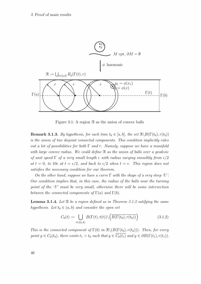
3 Proof of main results
φ harmonic
M cpt, ∂M = ∅
R :=⋃t∈[a,b] Bg(Γ(t), r)
r r r y1 = φ(x1)y = φ(x)
x1x
Γ(a) Γ(t)Γ(b)
Figure 3.1: A region R as the union of convex balls
Remark 3.1.3. By hypothesis, for each time t0 ∈ [a, b], the set R\B(Γ(t0), r(t0))
is the union of two disjoint connected components. This condition implicitly rules
out a lot of possibilities for both Γ and r. Namely, suppose we have a manifold
with large convex radius. We could define R as the union of balls over a geodesic
of unit speed Γ of a very small length ε with radius varying smoothly from ε/2
at t = 0, to 10ε at t = ε/2, and back to ε/2 when t = ε. This region does not
satisfies the necessary condition for our theorem.
On the other hand, suppose we have a curve Γ with the shape of a very steep ‘U ’.
Our condition implies that, in this case, the radius of the balls near the turning
point of the ‘U’ must be very small, otherwise there will be some intersection
between the connected components of Γ(a) and Γ(b).
Lemma 3.1.4. Let R be a region defined as in Theorem 3.1.2 satifying the same
hypothesis. Let t0 ∈ (a, b) and consider the open set
Cb(t) :=⋃
t∈[t0,b)
B(Γ(t), t(t))\(B(Γ(t0), r(t0))
)(3.1.2)
This is the connected component of Γ(b) in R\(B(Γ(t0), r(t0))). Then, for every
point y ∈ Cb(t0), there exists t1 > t0 such that y ∈ Cb(t1) and y ∈ ∂B(Γ(t1), r(t1)).
46

3.1 The Geometry of the Maximum Principle
Proof. By definition of Cb(t), whenever s′ > s, we have Cb(s′) ( Cb(s). Since
Cb(t0) is an open set, there exists δ > 0 such that B(y, δ) ⊂ Cb(t0). Therefore, as
r is a smooth function of t, there exists δ(δ, t0) > 0 such that y ∈ Cb(t′), where
t′ := t0 + δ. Moreover, the set
A =t ∈ [t0 + δ, b− δ] | y ∈ Cb(t)
is non-empty, since t′ ∈ A. Now set t1 = max(A) and the lemma follows.
Proof of Theorem 3.1.2: (See Figure 3.1) We argue by contradiction. Suppose
that there exists a compact manifold (M, g) and a non-constant harmonic map
φ : M −→ N such that φ(M) ⊂ R. Let φ(x) = y ∈ R be a point in φ(M). By
definition of R and the fact that φ is non-constant, there exists t0 ∈ [a, b] such
that,
y ∈ ∂B(Γ(t0), r(t0)) ∩ Cb(t0),
where Cb(t) is defined by Equation (3.1.2). Therefore, by Sampson’s maximum
principle, for every open neighborhood Ux of x in M ,
φ(Ux) * B(Γ(t0), r(t0))
That is, there exists x1 ∈ Ux such that φ(x1) = y1 is mapped to the convex side
of B(Γ(t0, r(t0))). Moreover, as we assume that R\B(Γ(t0), r(t0)) is disconnected,
y1 ∈ Cb(t0). Therefore, by Lemma 3.1.4, there exists a t1 > t0 such that
y1 ∈ ∂B(Γ(t1), r(t1)) ∩ Cb(t1)
Again, by Sampson’s maximum principle, every open neighborhood Ux1 of x1 in
M satisfies
φ(Ux1) * B(Γ(t1), r(t1)),
that is, there exists x2 ∈ Ux1 such that φ(x2) =: y2 /∈ B(Γ(t1), r(t1)), y2 is in the
convex side of ∂B(Γ(t1), r(t1)) and in the same connected component as Γ(b). By
induction, we construct a sequence yi, tii∈N, such that for every i ∈ N we have
ti > ti+1, limi→+∞ ti = b, yi ∈ φ(M), and yi ∈ Cb(ti). Since
Cb(ti) ( Cb(ti−1),
it follows that, denoting y∞ = limi→+∞ yi, that y∞ ∈ ∂B(Γ(b), r(b)) ∩ ∂R. Once
more, by Sampson’s maximum principle at y∞ = φ(x∞), every neighborhood
Ux∞ of x∞ in M has a point x′ such that φ(x′) = y′ is in the convex side of
∂B(Γ(p), r(p)) ∩ ∂R. Therefore y′ = φ(x′) /∈ R.
47

3 Proof of main results
p
A(p)
Figure 3.2: S2\(
12Eq)ε
This result has interesting applications.
Example 3.1.5. Let (N, h) = (S2, g) ⊂ (R3, geuc) and let Γ : [0, 1] −→ S2
be the unit speed geodesic such that Γ(0) = (−1, 0, 0), Γ(1/2) = (0, 0, 1) and
Γ(1) = (1, 0, 0). For a given ε > 0, let
R :=⋃t∈[0,1]
B(
Γ(t),π
2− ε
2
)(3.1.3)
and note that R contains the complement of an ε-neighborhood of the half equator
containing the points (0, 0,−1), (0,−1, 0) and (0, 1, 0), denoted by 12Eq. We write
R as S2\(
12Eq)ε. Theorem 3.1.2 implies that S2\
(12Eq)ε
has property (?).See
Figure 3.2.
Remark 3.1.6. The above argument also works for spheres Sn when we take out
a closed half equator, denoted by 12Sn−1. This result appears in [JXY12], where a
strictly convex function on each compact subset properly contained in Sn\12Sn−1
is constructed.
Remark 3.1.7. The main idea of the proof of Theorem 3.1.2 is that ∂R is a
barrier to the existence of non-constant harmonic maps. With the help of the
Sampson’s maximum principle, from now on abbreviated by SMP and the definition
48

3.1 The Geometry of the Maximum Principle
of R as a union of convex balls, we push the image of the harmonic map to this
barrier.
One can make the theorem more general by replacing ∂R ∩ ∂B(Γ(b), r(b)) with
some more flexible barrier. For example, with the family of balls defined in
Example 3.1.5, one would prove that there are no non-constant harmonic maps
whose image is contained in an open subset of S2\γ where γ is a connected curve
connecting the antipodal points (0, 1, 0), (0,−1, 0) ∈ S2.
Note that the classical method used to prove non-existence of such non-constant
harmonic maps, the method of looking for a strictly convex function f : R −→ R(in the geodesic sense), is not very flexible. Once one changes the boundary of R
slightly, one can no longer guarantee that there exists a strictly convex function
f : R −→ R.
3.1.2 Barriers to the existence of harmonic maps
Our proof of Theorem 3.1.2 gave the barrier for the existence of harmonic maps
as the boundary of the union of a family of balls whose centers are given by a
smooth embedded curve.
By studying barriers to the existence of harmonic maps abstractly, we find that
the result does not rely on the existence of such a family of balls along a curve.
The region R defined in Example 3.1.5 contains no closed geodesics, and since
geodesics are harmonic maps, it is necessary to avoid them for the non-existence
of non-constant harmonic maps. Therefore the first condition we are looking for
is one that avoids such curves.
Condition 1. For every p ∈ R and every v ∈ T 1pN , the geodesic Γ such that
Γ(0) = p and Γ′(0) = v satisfies, for some tv ∈ [0, K], Γ(tv) ∈ ∂R, where K is
independent of p and v.
Condition 1 is a qualitative way of imposing the non-existence of closed geodesics
in our region. But imposing the non-existence of closed geodesics in a given
region is not enough to avoid existence of harmonic maps, therefore we need an
extra condition to be stated later. But first, let us introduce some notation.
Notation 3.1.8. For p ∈ N and v ∈ TpN , we denote by γp,v : R −→ N the
geodesic that satisfies γp,v(0) = p and γ′p,v(0) = v.
As an example, suppose we have a point in the image of some geodesic, namely
Γp,v(t0). Take a tangent vector η ∈ TΓp,v(t0)N such that η 6= Γ′p,v(t0). If we
49

3 Proof of main results
consider another geodesic passing through Γp,v(t0) in the direction η at t = 0 ,
we write γΓp,v(t0),η(·) : R −→ N .
Notation 3.1.9. For p ∈ N , ν ∈ ∂Bg(p, r) with r 1, let tmax(p, ν) ∈ R+ be
the first time at which Γp,ν(t) ∈ ∂R.
We impose the following condition on the region R.
Condition 2. For every p ∈ R and every ν ∈ T 1pN , if t < tmax(p, ν), then the set
of directions η ∈ T 1Γp,ν(t)N such that d
(p, γRΓp,ν(t),η(ε)
)< d(p,Γp,ν(t)) is properly
contained in T 1Γp,ν(t) and connected. Here γR denotes a geodesic in R with ε ∈ R+
sufficiently small (that is, a curve that minimizes the length in R).
On one hand, Condition 2 is difficult to check unless N is a symmetric space.
On the other hand, in view of the example given in Chapter 1, Section 1.2.1 on
the existence of a non-trivial harmonic map from a genus two surface into S2,
we must have a very restrictive condition on R, namely Condition 2, to obtain a
result on the existence of harmonic maps as general as the one stated below.
Theorem 3.1.10. Let (N,h) be a complete Riemannian manifold and suppose
that for a region R ⊂ N , we have that R \ ∂R is open and connected. In addition,
suppose R satisfies the Conditions 1 and 2 above. Then R has property (?) of
Definition 1.4.1.
Proof. We argue by contradiction. Suppose that there exists a compact manifold
(M, g) and a non-constant harmonic map φ : M −→ N such that φ(M) ⊂ R.
Therefore, there exist points p = φ(x), q ∈ R such that d(q, p) 1 and a geodesic
Γ with Γ(0) = p, Γ′(0) = vp,q, and Γ(tp) = q. By Condition 1 there exists
tvp,q ∈ R+ such that Γ intersects ∂R. Define
Q0 := ∪t∈R+B(Γ(t), δ) with δ > δ0 > 0
and note that it satisfies the conditions of Theorem 3.1.2.
Therefore, when walking along Γ with the ball B(Γ(t), δ), there exists q1 /∈ Q0
such that q1 = φ(y1), y1 ∈M , and Condition 2 tells us that
dR(q1, p) > dR(q, p).
Let γR1 be a curve in R, connecting p and q1, of minimal length. Note that it
may not be a geodesic in N itself. By Condition 2, there exists η1 ∈ T 1q1N such
that Γq1,η1 increases the distance to p, that is
dR(Γq1,η1(t), p) > dR(q1, p)
50

3.1 The Geometry of the Maximum Principle
for sufficiently small t. As before, Γq1,η1 hits the boundary at some point tq1 by
Condition 1.
Let
Q1 := ∪t∈R+B(Γq1,η1(t), δ1), δ1 > δ0.
By Theorem 3.1.2, there exist q2 ∈ Q1 such that q2 = φ(y2) and
dR(q2, p) > dR(q1, p) > dR(q, p).
Inductively, we build a sequence of points q1, q2, q3, ... such that qi = φ(yi) with
yi ∈M for all i ∈ N and
dR(qi, p) = dR(qi, φ(x)) > dR(qi−1, φ(x)).
We claim that there exists k ∈ N such that qk /∈ R. Namely, by the compactness
of φ(M)∩R, the only possibility for this sequence to stay inside R is if there is q ∈ R
such that qi −→ q. Suppose this happens, then we can take a sufficiently small
ε > 0 such that dR(qi, q) < ε and consider the geodesic Γqi→q in N with Γqi(0) = qi
and Γ′qi(0) = νqi→q. The construction of a region Q1 := ∪t∈R+B(Γqi→q(t), δ) would
give us q1 = φ(y1) such that dR(p, q1) > dR(p, q), and we can continue invoking
this argument. Induction implies that such a k ∈ N exists.
Example 3.1.11. One can use the above theorem to find regions in symmetric
spaces for which property (?) holds. If one has some information on the geometry
of such a space, Conditions 1 and 2 may be easy to check. For instance, let
p ≥ 1 and (Σp, g) be a compact surface of genus p with a hyperbolic metric of
constant curvature. Let γ1, ..., γ2p be smooth curves that generate H1(Σp,R), the
first homology group of Σp. For a given ε > 0, define
R := Σp\(γ1 ∪ ... ∪ γ2p)ε (3.1.4)
We see that R satisfies Conditions 1 and 2, therefore it has property (?). See
Figure 3.3.
An alternative proof of this statement could be given by noting that a harmonic
map defined on a compact manifold and taking values in a polygon with 4p sides
in the Poincare hyperbolic space such that its image is contained in the interior
of this polygon must be constant. The example above illustrates the relation
between properties of harmonic maps and maximum principles.
Remark 3.1.12 (Property (?) for graphs). To use the previous results to obtain
Bernstein-type theorems we have to overcome the compactness of M . We will
51

3 Proof of main results
φ
harmonic
M compact
∂M = ∅
Figure 3.3: Example of barriers for the existence of harmonic maps in immersed
surfaces in R3 of genus one, two and three.
be able to do so for the graph case. More precisely, we will impose the following
conditions on M : Let M = graph(f) be a minimal submanifold, where f : Rp −→Rn, and γ : M −→ G+
p,n is its Gauss map. Suppose γ(M) ⊂ R, where R is a
region in G+p,n that has property (?). As pointed out by Fischer-Colbrie in [FC80],
one can use Allard’s general work on varifolds to prove that the tangent cone at
infinity of a manifold M given by the graph of a smooth map is the cone over
a compact minimal submanifold M of the sphere [All72]. The Gauss map of
M is again harmonic and satisfies γ(M) ⊂ R. Once more, by an argument of
Fischer-Colbrie [FC80], the compactness of M implies that γ is constant. Hence,
M is the graph of a linear map.
We study the geometry of Grassmannians in detail because we want to explicitly
understand regions in G+p,n that have Property (?) and conditions on the Gauss
map of a manifold that guarantee that its image is contained in such a region.
3.2 Bernstein-type theorems for codimension 2
In this section we construct regions in Grassmannian manifolds that have property
(?) for graphs and use them to prove Bernstein-type theorems. First, we need to
explain the relation of the geometry of Gauss maps with the slope of graphs. To
show the gist of our method, we first explain how Moser’s Bernstein theorem for
52

3.2 Bernstein-type theorems for codimension 2
p
A(p)
p
A(p)
Figure 3.4: (12Eq)ε × (1
2Eq)ε remains as a barrier in S2 × S2.
codimension 1 follows from our method. Then we proceed to derive an analogous
result in codimension 2.
We want to use the geometry of Grassmannians to construct regions in G+p,p+2
satisfying Conditions 1 and 2 of Theorem 3.1.10, to conclude that these regions
have property (?).
Let us start with the simplest case, the manifold (S2 × S2, g × g) which is
isometric to G+2,4 with its standard metric. By Example 3.1.5, we know that
S2\(12Eq)ε has property (?). We define R :=
(S2\(1
2Eq)ε × (S2\(1
2Eq)ε)
)and
look at a given geodesic in S2 × S2:
γ :R −→ S2 × S2
t 7→ (γ1(t), γ2(t)).(3.2.1)
Here γ1, γ2 : R −→ S2 are two geodesics in S2. Therefore R satisfies Conditions 1
and 2 of Theorem 3.1.10 (actually, Theorem 3.1.2 already suffices to see that R is
a barrier) and therefore R has property (?) as well. See Figure 3.4.
By Equation (2.3.31), if Σ2 = (x, f(x)) is an embedded minimal surface in R4
where f : R2 −→ R2 is a smooth mapping with slope ∆f < β0 < +∞, then the
harmonic Gauss map γ : Σ2 −→ G+2,4 maps into the above region, i.e., γ(Σ2) ⊂ R.
Now, by Remark 3.1.12, we have that γ is constant, implying that Σ2 is a plane
in R4.
For the more general case where n = p + 2, we proceed as follows. Write
w ∈ G+p,p+2 ⊂ S(p+2
p )−1 as w = e1 ∧ ... ∧ ep, where eipi=1 is an orthonormal basis
for Vw and n1, n2 an orthonormal basis for V ⊥w . In TwG+p,p+2 there are p(p−1)
2
53

3 Proof of main results
vectors of type 2 (as ∧ anti-commutes), we denote them by X i2, i = 1, ..., p(p−1)
2.
For a given ε > 0, define
R :=
p(p−1)2⋃i=1
⋃−tXi2
+ε<t<tXi2−ε
BG
(wXi
2(t)). (3.2.2)
Since G+p,p+2 is a homogeneous space of non-negative curvature and the geodesics
are given by Equation (2.3.15), we have that R satisfies Condition 2 in section
3, that is, for a given w ∈ R, up to time t < tXj , j = 1, 2, there is always a
direction where the distance to w increases. On the other hand, as we take the
union over −tX2 + ε < t < tX2 − ε (i.e. strictly smaller than the critical time),
we are excluding the points where 〈w,wXi2(t)〉 = cos2(t/
√2) = 0. Therefore
〈w,wXi2(t)〉 > 0 for all i = 1, ..., p(p− 1)/2 and there are no closed geodesics in R
centered at any point w ∈ R. Once more, as G+p,p+2 ⊂ S(p+2
p )−1 is a symmetric
space, w−Xi2(t) = wXi
2(−t), and we have that the only points in wXi
2(R) we are
excluding are the ones that are ε-close to the equator with respect to w in S(p+2p )−1,
thus R =(G+p,p+2\Hem(−w)
)ε
has property (?) and hence, by Remark 3.1.12,
property (?) for graphs, for every ε > 0.
Once more, by Equation (2.3.31), if Mp = (x, f(x)) is an embedded minimal
submanifold in Rp+2 and f is a smooth mapping with slope ∆f < β0 < +∞,
then the harmonic Gauss map γ : Mp −→ G+p,p+2 satisfies γ(Mp) ⊂ R. Thus γ is
constant and Mp is a plane in Rp+2.
Remark 3.2.1. If n ≥ p + 3, the definition of such a region R would have to
include not only the union over directions of type 3 (and more), but unions over
type 2 vectors in directions of type 1, and so on. For example, once we transport
a type 1 vector along a geodesic with tangent vector of type 3, we may obtain a
type 2 vector and hence we have to verify whether this would give us a closed
geodesic in R. It can be proven that in general a closed geodesic exists inside R if
we take the union over all directions in higher codimensions. Therefore a more
refined definition of such a region in higher codimension is necessary, as follows
from the existence of the Lawson-Osserman cone.
Returning to codimension 2, the above discussion yields the following theorem,
which extends Moser’s result from codimension 1 to codimension 2.
Theorem 3.2.2. Let zi = f i(x1, ..., xp), i = 1, 2, be smooth functions defined
everywhere in Rp. Suppose their graph M = (x, f(x)) is a submanifold with
54

3.2 Bernstein-type theorems for codimension 2
parallel mean curvature in Rp+2. Suppose that there exists a number β0 < +∞such that
∆f (x) ≤ β0 for all x ∈ Rn, (3.2.3)
where
∆f (x) :=
det
(δαβ +
∑i
f ixα(x)f ixβ(x)
) 12
. (3.2.4)
Then f 1, f 2 are linear functions on Rp representing an affine p-plane in Rp+2.
55


4 Open problems
This chapter presents some problems that arise from this dissertation and that
the author intends to work on in the future.
4.1 Convex supporting domains
In Chapter 2, we defined the concept of a convex supporting domain. Namely,
let (N, h) be a Riemannian manifold and V ⊂ N . We say that V is a convex
supporting domain if there exists a strictly convex function f : V −→ R. The
maximum principle 2.1.6 implies the following:
For V ⊂ N, there exists a striclty convex function f : V −→ R⇓ ⇑?
There is no compact M and harm. non-const. φ : M → N such that φ(M) ⊂ V
⇓ ⇑?
There is no n ≥ 1 and harm. non-const. φ : Sn → N such that φ(Sn) ⊂ V
⇓ ⇑?
There is no harm. non-const. φ : S1 → N such that φ(M) ⊂ V
Emery conjectured that if a subset V ⊂ N admits no closed geodesics, that is,
if every harmonic map φ : S1 → N such that φ(S1) ⊂ V is a constant map,
then there exists a strictly convex function f : V → R [Ken90], [CK99]. This
conjecture is refuted by the example we have given in Chapter 1 regarding the
existence of a non-constant harmonic map into S2\(Γ1 ∪ Γ2 ∪ Γ3). What about
all the other reverse implications?
We conjecture that the first reverse implication holds true. Namely, suppose
V ⊂ has property (?), then there exists a strictly convex function f : V → N .
A complete answer to all the implications on this diagram would be a powerful
result. On one hand, it is a problem interesting on its own. On the other hand,
since in this thesis we have given abstract ways of showing that a region has
property (?), this would give us a conceptual way of verifying whether a region
does admit a strictly convex function.
57

4 Open problems
4.2 Bernstein theorems for codimension c ≥ 3
Our methods to obtain regions without images of harmonic maps can be applied
in general complete manifolds, therefore in Grassmannian manifolds of arbitrary
dimensions. In this case it is important to understand the behavior of closed
geodesics in such manifolds. Of course, as we explained in detail, if the codimension
is one, the Grassmannian is just a sphere and closed geodesics are great circles. If
the codimension is two, there are closed geodesics with more interesting geometry.
For instance, the Grassmannian
G+p,p+2 ⊂ S(p+2
p )−1
contains closed geodesics in the north hemisphere of S(p+2p )−1.
The geodesic equations obtained in [Koz97] for Grassmannians, which we used
in [AJ18] to obtain Moser’s Bernstein theorem in codimension 2, can also be used
to study the case of c ≥ 3. The natural questions are:
• Can we obtain bounds closer to the counterexamples of Lawson and Os-
sermann [LO77], by a systematical study of geodesics in Grassmannians of
arbitrary dimensions?
• Based on [JXY16], it seems that Lawson-Osserman cones are not a sharp
counterexample to Bernstein’s theorem in higher codimension. Can we use
similar methods to the ones in [AJ18] to obtain ‘sharper cones’?
Let us give a very brief description of why the problem becomes more difficult in
codimension 3.
To deal with the closed geodesics that appear in the hemisphere of a given
point, we counted all the possible directions that could occur and since the type
2 vectors were the worse case, of which there are just(p+2
2
), we could handle the
problem. Now, we have an extra codimension. Therefore we must control what
happens to the closed geodesics that have as tangent vector the parallel transport
of a type 2 vector along some other curve (geodesic) that has a type 3 vector as
the tangent direction. On the other hand, the same can happen if we parallel
transport a type 3 vector in a type 1 direction and suddenly obtain a problematic
type 2 vector. This could give us closed geodesics inside our region R.
This is a paper in preparation. We are computing examples similar to Exam-
ples 2.3.19 and 2.3.20, but now also carrying out the parallel translation along
58

4.2 Bernstein theorems for codimension c ≥ 3
other type k vectors to obtain the bounds of the desired region and hence the
bounds for a Bernstein-type theorem.
We have geometrical evidences suggesting that Lawson-Osserman cones are
not the optimal counterexamples to Bernstein theorems in higher codimensions.
Hopefully, further work will be done in this direction.
4.2.1 Non-smooth setting
So far, we have only dealt with smooth manifolds. As pointed out in the previous
section, the main tool used in [AJ18] was the Sampson maximum principle.
Thanks to White [Whi09], we know that there exists an equivalent of this theorem
in the case of minimal varifolds.
A powerful method to study minimal submanifolds is to consider their cone at
infinity, which happens to be a varifold.
• Can we develop similar techniques to the ones in [AJ18] to understand the
existence of stable varifolds on a given manifold?
• How can this result lead to more general Bernstein-type problems?
59


Bibliography
[AJ18] Renan Assimos and Jurgen Jost. The geometry of maximum principles
and a Bernstein theorem in codimension 2. 2018. Submitted. Preprint
available on arXiv:1811.09869.
[All72] William K. Allard. On the first variation of a varifold. Annals of
Mathematics, 95(3):417–491, 1972.
[BDGG69] Enrico Bombieri, Ennio De Giorgi, and Enrico Giusti. Minimal cones
and the Bernstein problem. Inventiones mathematicae, 7(3):243–268,
1969.
[Ber15] Sergei Natanovich Bernstein. Sur un theoreme de geometrie et son
application aux equations aux derivees partielles du type elliptique.
Communications de la Societe mathematique de Kharkow, 15(1):38–45,
1915.
[Che65] Shiing-shen Chern. On the curvatures of a piece of hypersurface in
Euclidean space. In Abhandlungen aus dem Mathematischen Seminar
der Universitat Hamburg, volume 29, pages 77–91. Springer, 1965.
[CK99] Jose Manuel Corcuera and Wilfrid S Kendall. Riemannian barycentres
and geodesic convexity. In Mathematical Proceedings of the Cam-
bridge Philosophical Society, volume 127, pages 253–269. Cambridge
University Press, 1999.
[CX92] Q Chen and YL Xin. A generalized maximum principle and its applica-
tions in geometry. American Journal of Mathematics, 114(2):355–366,
1992.
[DdPW17] Juan Davila, Manuel del Pino, and Juncheng Wei. Singularity for-
mation for the two-dimensional harmonic map flow into s2. arXiv
preprint arXiv:1702.05801, 2017.
61

BIBLIOGRAPHY
[DHS10] Ulrich Dierkes, Stefan Hildebrandt, and Friedrich Sauvigny. Minimal
surfaces. In Minimal Surfaces, pages 53–90. Springer, 2010.
[FC80] Doris Fischer-Colbrie. Some rigidity theorems for minimal submani-
folds of the sphere. Acta Mathematica, 145(1):29–46, 1980.
[Hel02] Frederic Helein. Harmonic maps, conservation laws and moving
frames, volume 150. Cambridge University Press, 2002.
[HJW80] Stefan Hildebrandt, Jurgen Jost, and K-O Widman. Harmonic map-
pings and minimal submanifolds. Inventiones mathematicae, 62(2):269–
298, 1980.
[Jos91] Jurgen Jost. Two-dimensional geometric variational problems. Pure
Appl. Math.(NY), 1991.
[Jos08] Jurgen Jost. Riemannian geometry and geometric analysis, volume
42005. Springer, 2008.
[Jos12] Jurgen Jost. Nonpositive curvature: geometric and analytic aspects.
Birkhauser, 2012.
[JX99] Jurgen Jost and Yuan-Long Xin. Bernstein type theorems for higher
codimension. Calculus of variations and Partial differential equations,
9(4):277–296, 1999.
[JXY12] Jurgen Jost, Yuanlong Xin, and Ling Yang. The regularity of harmonic
maps into spheres and applications to Bernstein problems. Journal
of Differential Geometry, 90(1):131–176, 2012.
[JXY16] Jurgen Jost, Yuan Long Xin, and Ling Yang. The Geometry of
Grassmannian manifolds and Bernstein type theorems for higher
codimension. Annali della Scuola Normale Superiore di Pisa. Classe
di scienze, 16(1):1–39, 2016.
[Ken90] Wilfrid S Kendall. Probability, convexity, and harmonic maps with
small image i: uniqueness and fine existence. Proceedings of the
London Mathematical Society, 3(2):371–406, 1990.
[Koz97] Sergey Emel’yanovich Kozlov. Geometry of the real Grassmannian
manifolds. Parts I, II and III. Zapiski Nauchnykh Seminarov POMI,
246:84–129, 1997.
62

BIBLIOGRAPHY
[Lem78] Luc Lemaire. Harmonic nonholomorphic maps from a surface to a
sphere. Proceedings of the American Mathematical Society, 71(2):299–
304, 1978.
[LO77] H Blaine Lawson and Robert Osserman. Non-existence, non-
uniqueness and irregularity of solutions to the minimal surface system.
Acta Mathematica, 139(1):1–17, 1977.
[LW08] Fanghua Lin and Changyou Wang. The analysis of harmonic maps
and their heat flows. World Scientific, 2008.
[Mos61] Jurgen Moser. On Harnack’s theorem for elliptic differential equations.
Communications on Pure and Applied Mathematics, 14(3):577–591,
1961.
[Oss02] Robert Osserman. A survey of minimal surfaces. Courier Corporation,
2002.
[RV70] Ernst A Ruh and Jaak Vilms. The tension field of the Gauss map.
Transactions of the American Mathematical Society, 149(2):569–573,
1970.
[Sim68] James Simons. Minimal varieties in Riemannian manifolds. Annals
of Mathematics, pages 62–105, 1968.
[Str85] Michael Struwe. On the evolution of harmonic mappings of riemannian
surfaces. Commentarii Mathematici Helvetici, 60(1):558–581, 1985.
[SU81] Jonathan Sacks and Karen Uhlenbeck. The existence of minimal
immersions of 2-spheres. Annals of mathematics, pages 1–24, 1981.
[Whi09] Brian White. The maximum principle for minimal varieties of arbitrary
codimension. arXiv preprint arXiv:0906.0189, 2009.
[Xin03] Yuanlong Xin. Minimal submanifolds and related topics, volume 8.
World Scientific, 2003.
[Xin12] Yuanlong Xin. Geometry of harmonic maps, volume 23. Springer
Science & Business Media, 2012.
63


Selbststandigkeitserklarung
Hiermit erklare ich, die vorliegende Dissertation selbstandig und ohne un-
zulassige fremde Hilfe angefertigt zu haben. Ich habe keine anderen als die
angefuhrten Quellen und Hilfsmittel benutzt und samtliche Textstellen, die
wortlich oder sinngemaß aus veroffentlichten oder unveroffentlichten Schriften
entnommen wurden, und alle Angaben, die auf mundlichen Auskunften beruhen,
als solche kenntlich gemacht. Ebenfalls sind alle von anderen Personen bereit-
gestellten Materialien oder erbrachten Dienstleistungen als solche gekennzeichnet.
Leipzig, den 24.01.2019
. . . . . . . . . . . . . . . . . . . . . . . . . . .
(Renan Assimos Martins)


Daten zum Autor
Name: Renan Assimos Martins
Geburtsdatum: 22.05.1989 in Rio de Janeiro (Brasilien)
03/2010 - 08/2013 Bachelorstudium in Mathematik
Universidade Federal do Rio de Janeiro (Rio de Janeiro, Brasilien)
09/2011 - 05/2014 Masterstudium in Mathematik
Universidade Federal do Rio de Janeiro (Rio de Janeiro, Brasilien)
seit 02/2015 Doktorand im Fachgebiet Mathematik
Max-Planck Institut fur Mathematik in den Naturwissenschaften,
Universitat Leipzig