Embed Size (px)
Citation preview

The Bernstein polynomial basis:a centennial retrospective
a “sociological study” in theevolution of mathematical ideas
Rida T. Farouki
Department of Mechanical & Aerospace Engineering,University of California, Davis
— synopsis —
• 1912: Sergei Natanovich Bernstein —constructive proof of Weierstrass approximation theorem
• 1960s: Paul de Faget de Casteljau, Pierre Etienne Bezierand the origins of computer-aided geometric design
• elucidation of Bernstein basis properties and algorithms
• 1980s: intrinsic numerical stability of the Bernstein form
• algorithms & representations for computer-aided design
• diversification of applications in scientific computing
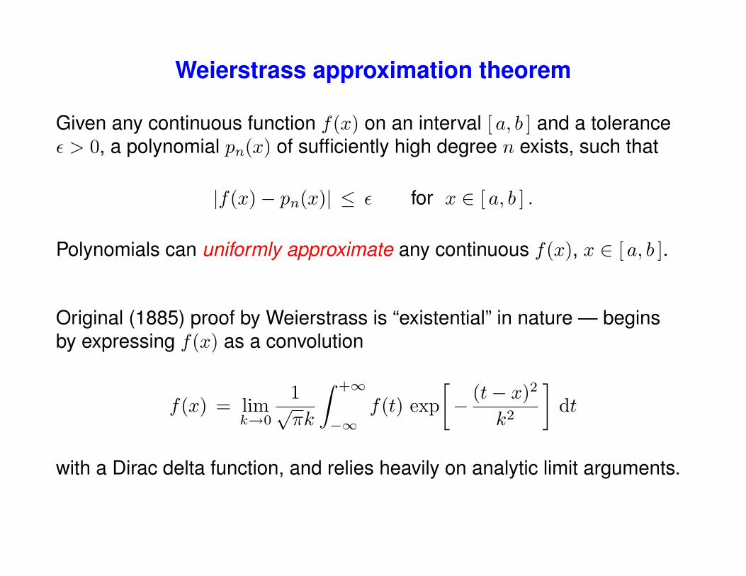
Weierstrass approximation theorem
Given any continuous function f(x) on an interval [ a, b ] and a toleranceε > 0, a polynomial pn(x) of sufficiently high degree n exists, such that
|f(x)− pn(x)| ≤ ε for x ∈ [ a, b ] .
Polynomials can uniformly approximate any continuous f(x), x ∈ [ a, b ].
Original (1885) proof by Weierstrass is “existential” in nature — beginsby expressing f(x) as a convolution
f(x) = limk→0
1√πk
∫ +∞
−∞f(t) exp
[− (t− x)2
k2
]dt
with a Dirac delta function, and relies heavily on analytic limit arguments.
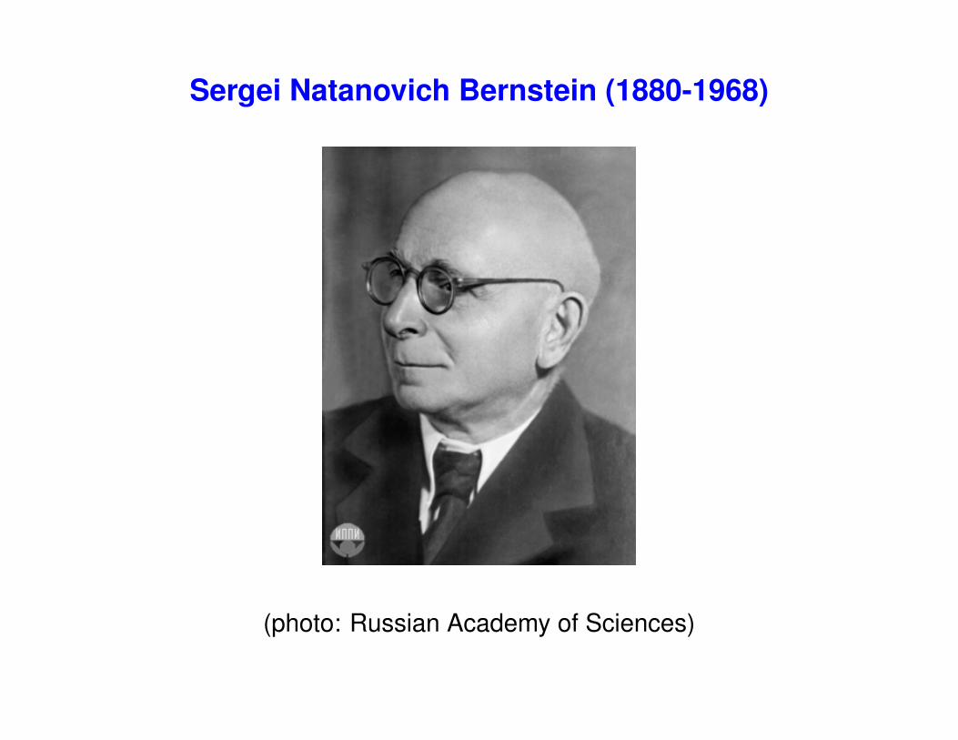
Sergei Natanovich Bernstein (1880-1968)
(photo: Russian Academy of Sciences)

academic career of S. N. Bernstein
• 1904: Sorbonne PhD thesis, on analytic nature of PDE solutions(worked with Hilbert at Gottingen during 1902-03 academic year)
• 1913: Kharkov PhD thesis (polynomial approximation of functions)
• 1912: Comm. Math. Soc. Kharkov paper (2 pages): constructiveproof of Weierstrass theorem — introduction of Bernstein basis
• 1920-32: Professor in Kharkov & Director of Mathematical Institutepolitical purge: moved to USSR Academy of Sciences (Leningrad)
• 1941-44: escapes to Kazakhstan during the siege of Leningrad
• 1944-57: Steklov Math. Institute, Russian Academy of Sciences,Moscow — edited complete works of Chebyshev (died 1968)
• collected works of Bernstein published in 4 volumes, 1952-64
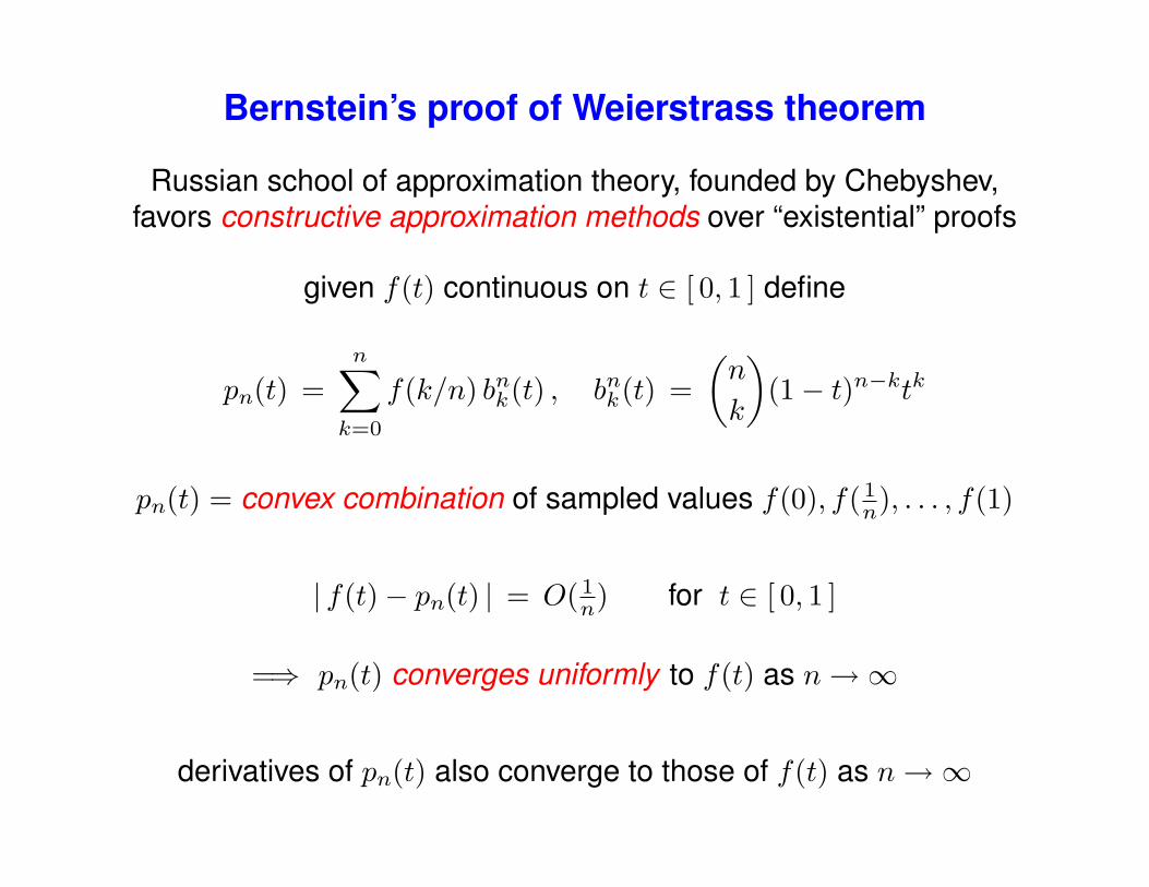
Bernstein’s proof of Weierstrass theorem
Russian school of approximation theory, founded by Chebyshev,favors constructive approximation methods over “existential” proofs
given f(t) continuous on t ∈ [ 0, 1 ] define
pn(t) =n∑k=0
f(k/n) bnk(t) , bnk(t) =(n
k
)(1− t)n−ktk
pn(t) = convex combination of sampled values f(0), f(1n), . . . , f(1)
| f(t)− pn(t) | = O(1n) for t ∈ [ 0, 1 ]
=⇒ pn(t) converges uniformly to f(t) as n→∞
derivatives of pn(t) also converge to those of f(t) as n→∞
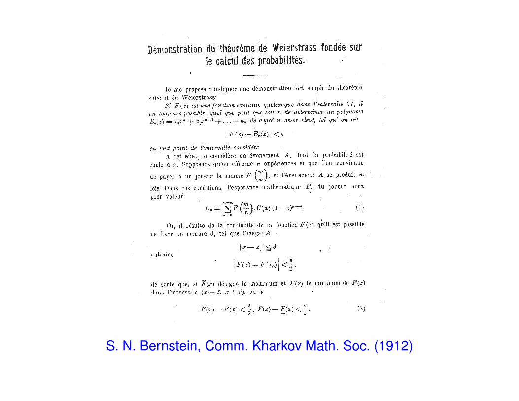
S. N. Bernstein, Comm. Kharkov Math. Soc. (1912)
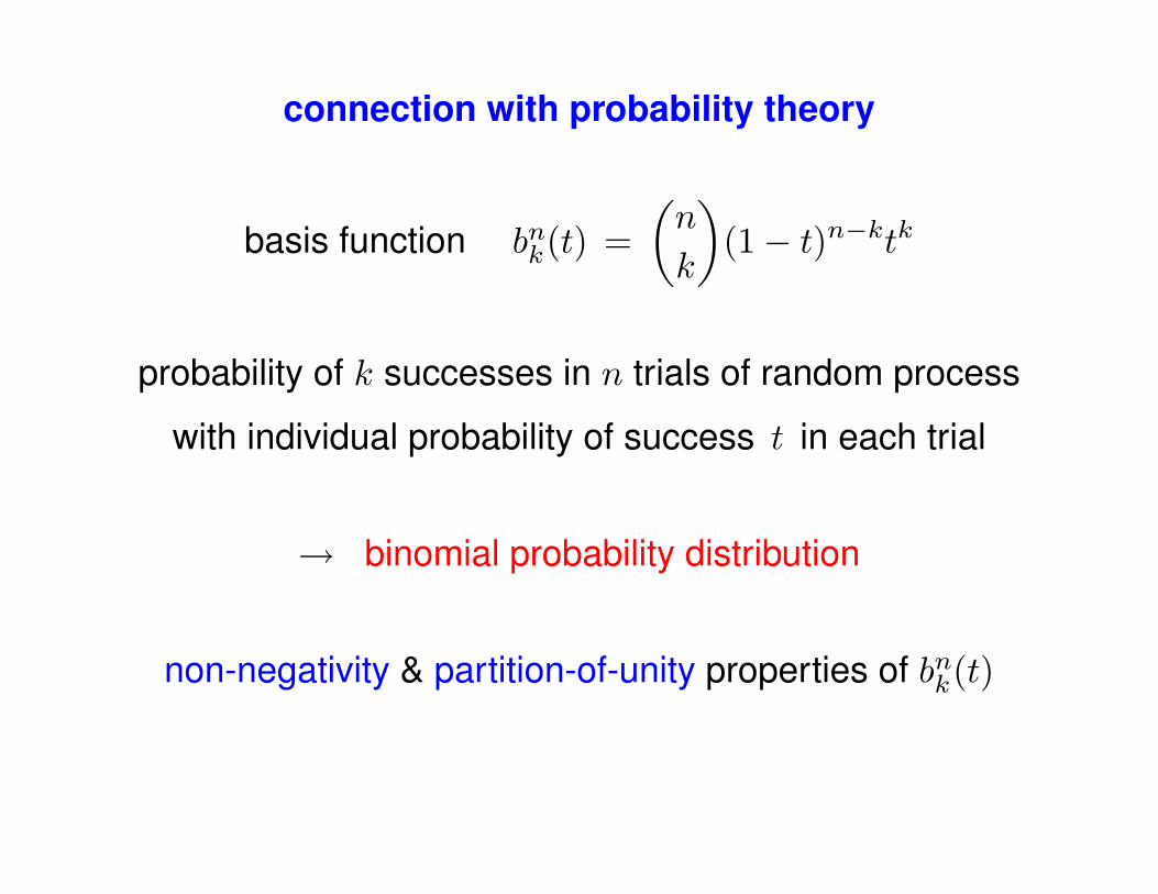
connection with probability theory
basis function bnk(t) =(n
k
)(1− t)n−ktk
probability of k successes in n trials of random process
with individual probability of success t in each trial
→ binomial probability distribution
non-negativity & partition-of-unity properties of bnk(t)
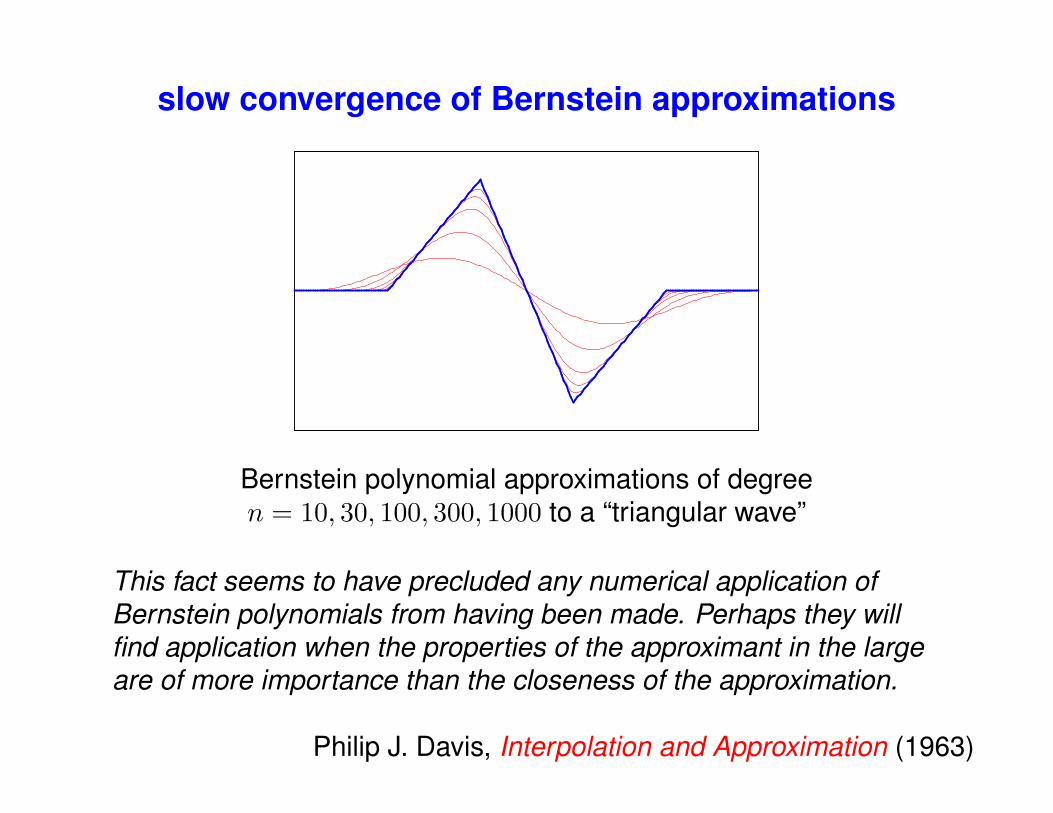
slow convergence of Bernstein approximations
Bernstein polynomial approximations of degreen = 10, 30, 100, 300, 1000 to a “triangular wave”
This fact seems to have precluded any numerical application ofBernstein polynomials from having been made. Perhaps they willfind application when the properties of the approximant in the largeare of more importance than the closeness of the approximation.
Philip J. Davis, Interpolation and Approximation (1963)

Paul de Casteljau & Pierre Bezier (1960s)an emerging application — computer-aided design
• Paul de Faget de Casteljau — theory of “courbes et surfaces a poles”developed at Andre Citroen, SA in the early 1960s
• de Casteljau’s work unpublised (regarded as proprietary by Citroen)— revealed to outside world by Wolfgang Bohm in mid-1980s
• Pierre Etienne Bezier — implemented methods for computer-aideddesign and manufacturing at Renault during 1960s and 1970s
• Bezier published numerous articles and books describing his ideas
• basic problem: provide intuitive & interactive means for design andmanipulation of “free–form” curves and surfaces by computer, in theautomotive, aerospace, and related industries
• identification of de Casteljau’s and Bezier’s ideas with Bernstein formof polynomials came later, through work of Forrest, Riesenfeld, et al.
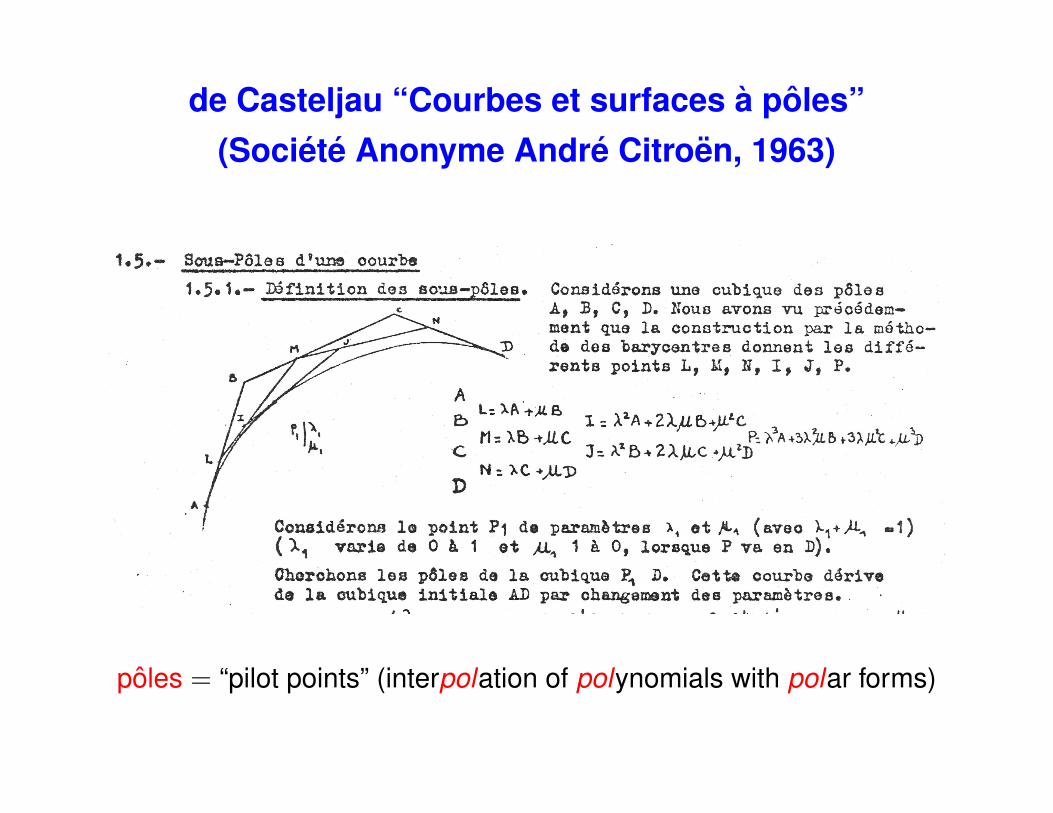
de Casteljau “Courbes et surfaces a poles”(Societe Anonyme Andre Citroen, 1963)
poles = “pilot points” (interpolation of polynomials with polar forms)
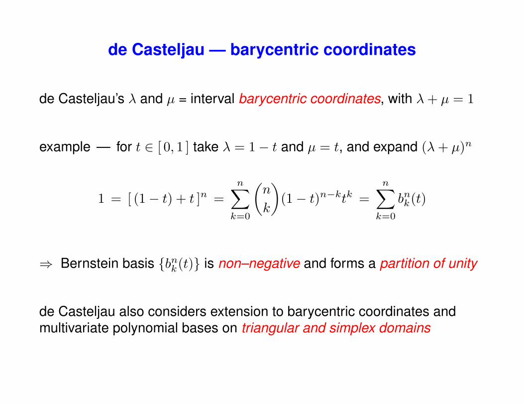
de Casteljau — barycentric coordinates
de Casteljau’s λ and µ = interval barycentric coordinates, with λ+ µ = 1
example — for t ∈ [ 0, 1 ] take λ = 1− t and µ = t, and expand (λ+ µ)n
1 = [ (1− t) + t ]n =n∑k=0
(n
k
)(1− t)n−ktk =
n∑k=0
bnk(t)
⇒ Bernstein basis {bnk(t)} is non–negative and forms a partition of unity
de Casteljau also considers extension to barycentric coordinates andmultivariate polynomial bases on triangular and simplex domains

computer-aided design in the early 60s
. . . the designers were astonished and scandalized. Was itsome kind of joke? It was considered nonsense to represent a carbody mathematically. It was enough to please the eye, the wordaccuracy had no meaning . . .
reaction at Citroen to de Casteljau’s ideas
Citroen’s first attempts at digital shape representation used a BurroughsE101 computer featuring 128 program steps, a 220-word memory, and a5 kW power consumption!
De Casteljau’s “insane” persistence led to an increased adoption ofcomputer-aided design methods in Citroen from 1963 onwards.
My stay at Citroen was not only an adventure for me,but also an adventure for Citroen! . . . . . . . . . . . . . . . . . . . . . . . P. de Casteljau
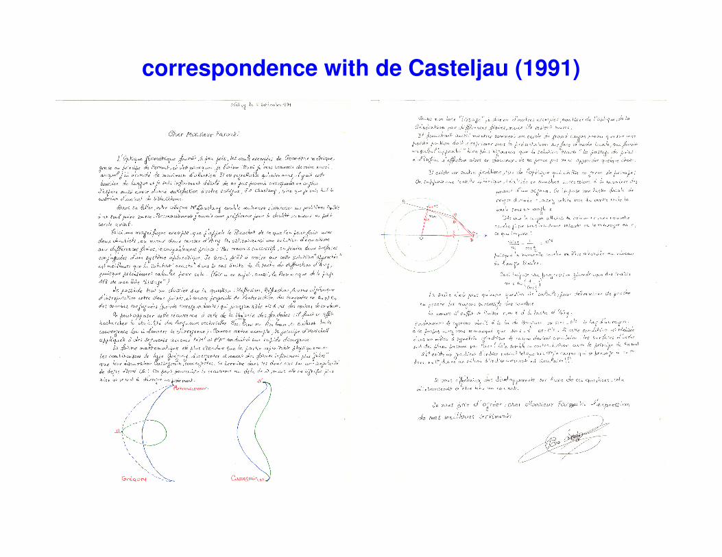
correspondence with de Casteljau (1991)
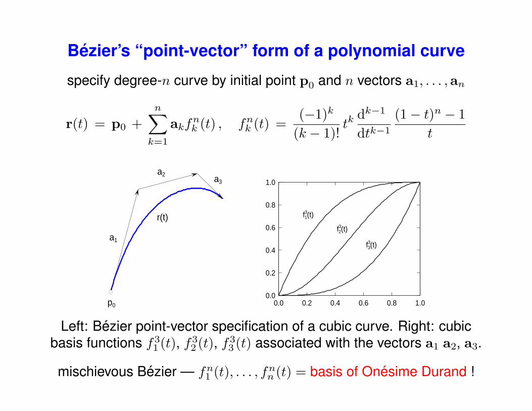
Bezier’s “point-vector” form of a polynomial curve
specify degree-n curve by initial point p0 and n vectors a1, . . . ,an
r(t) = p0 +n∑k=1
akfnk (t) , fnk (t) =(−1)k
(k − 1)!tk
dk−1
dtk−1
(1− t)n − 1t
0.0 0.2 0.4 0.6 0.8 1.00.0
0.2
0.4
0.6
0.8
1.0
p0
a1
a2a3
r(t) f31(t)
f32(t)
f33(t)
Left: Bezier point-vector specification of a cubic curve. Right: cubicbasis functions f3
1 (t), f32 (t), f3
3 (t) associated with the vectors a1 a2, a3.
mischievous Bezier — fn1 (t), . . . , fnn (t) = basis of Onesime Durand !
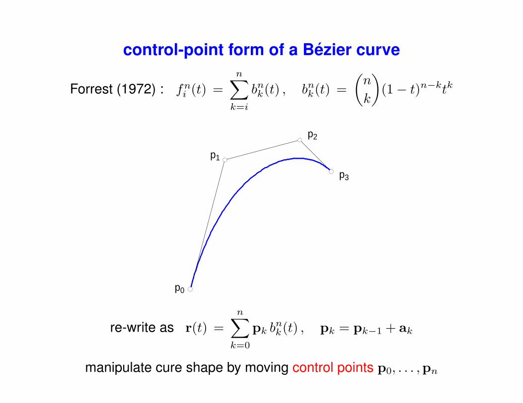
control-point form of a Bezier curve
Forrest (1972) : fni (t) =n∑k=i
bnk(t) , bnk(t) =(n
k
)(1− t)n−ktk
p0
p1
p2
p3
re-write as r(t) =n∑k=0
pk bnk(t) , pk = pk−1 + ak
manipulate cure shape by moving control points p0, . . . ,pn
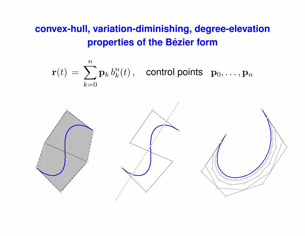
convex-hull, variation-diminishing, degree-elevationproperties of the Bezier form
r(t) =n∑k=0
pk bnk(t) , control points p0, . . . ,pn
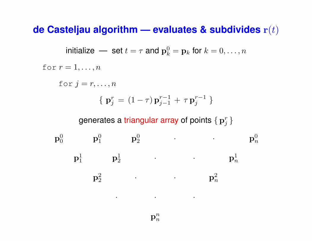
de Casteljau algorithm — evaluates & subdivides r(t)
initialize — set t = τ and p0k = pk for k = 0, . . . , n
for r = 1, . . . , n
for j = r, . . . , n
{ prj = (1− τ) pr−1j−1 + τ pr−1
j }
generates a triangular array of points {prj }
p00 p0
1 p02 · · p0
n
p11 p1
2 · · p1n
p22 · · p2
n
· · ·
pnn
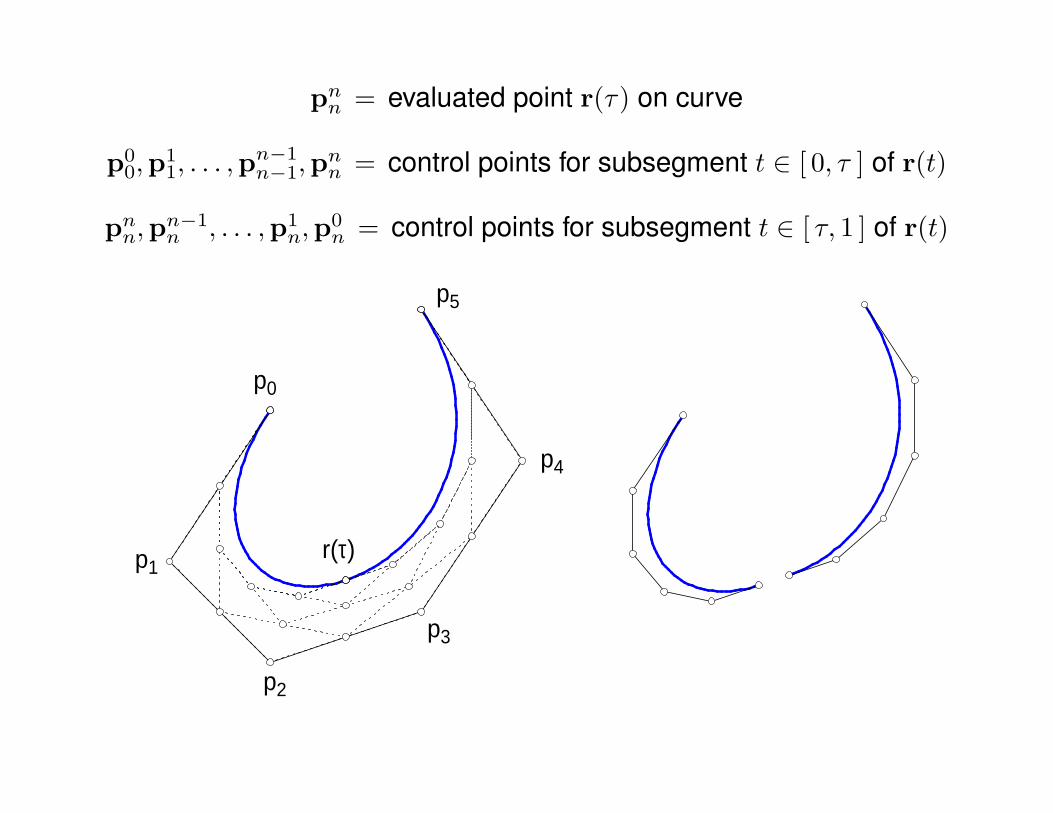
pnn = evaluated point r(τ) on curve
p00,p
11, . . . ,p
n−1n−1,p
nn = control points for subsegment t ∈ [ 0, τ ] of r(t)
pnn,pn−1n , . . . ,p1
n,p0n = control points for subsegment t ∈ [ τ, 1 ] of r(t)
r(τ)
p0
p1
p2
p3
p4
p5

interlude . . . “lost in translation”
warning sign on bathroom door in Beijing hotel

“English on vacation”
in a Bucharest hotel lobby —The elevator is being fixed for the next day.During that time we regret that you will be unbearable.
in a Paris hotel elevator —Please leave your values at the front desk.
in a Zurich hotel —Because of the impropriety of entertaining guests of the opposite sexin your bedroom, it is suggested that the lobby be used for this purpose.
in an Acapulco restaurant —The manager has personally passed all the water served here.
in Germany’s Schwarzwald —It is strictly forbidden on our Black Forest camping site that people ofdifferent sex — for instance, men and women — live together in one tentunless they are married with each other for that purpose.
in an Athens hotel —Guests are expected to complain at the office between 9 and 11 am daily.
instructions for AC in Japanese hotel —If you want just condition of warm in your room, please control yourself.
in a Yugoslav hotel —The flattening of underwear with pleasure is the job of the chambermaid.
in a Japanese hotel —You are invited to take advantage of the chambermaid.
on the menu of a Swiss restaurant —Our wines leave you nothing to hope for.
in a Bangkok dry cleaners —Drop your trousers here for best results.
Japanese rental car instructions —When passenger of foot heave in sight, tootle the horn.Trumpet him melodiously at first, but if he still obstaclesyour passage, then tootle him with vigor.
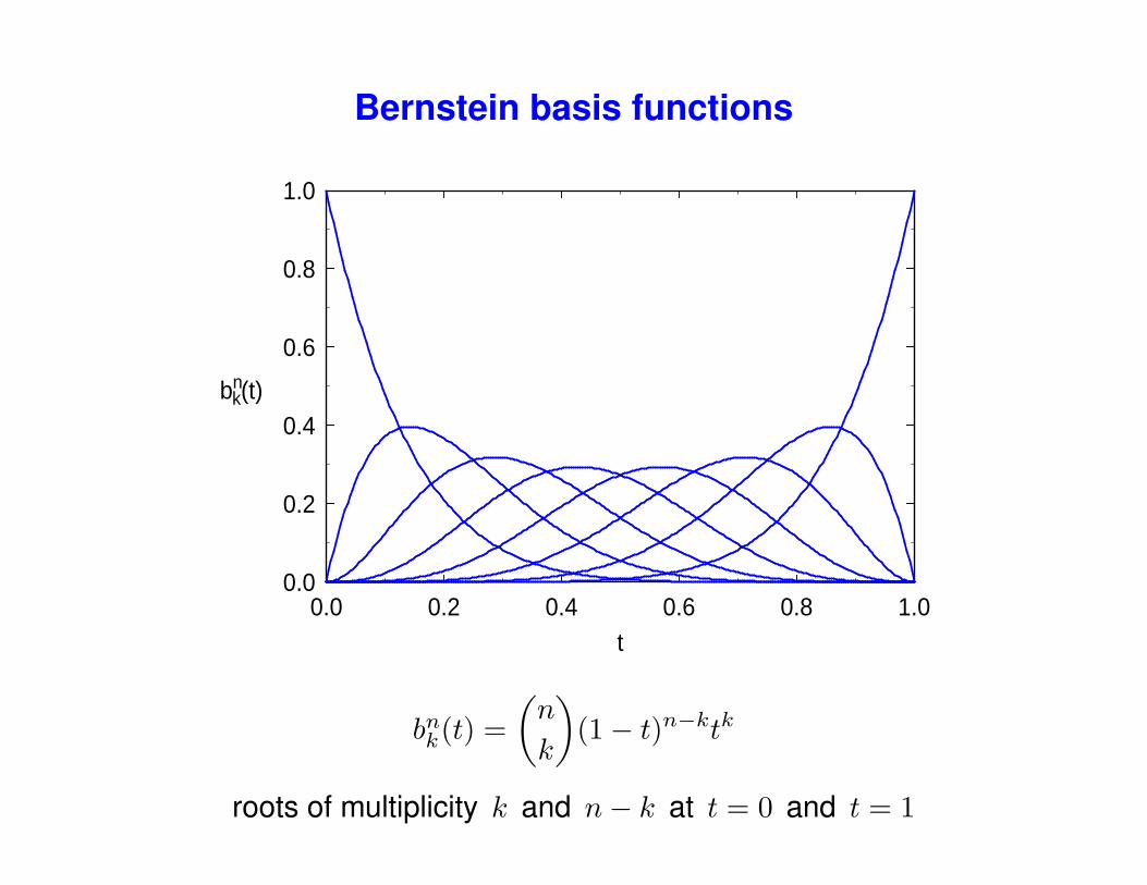
Bernstein basis functions
0.0 0.2 0.4 0.6 0.8 1.00.0
0.2
0.4
0.6
0.8
1.0
t
bnk(t)
bnk(t) =(n
k
)(1− t)n−ktk
roots of multiplicity k and n− k at t = 0 and t = 1
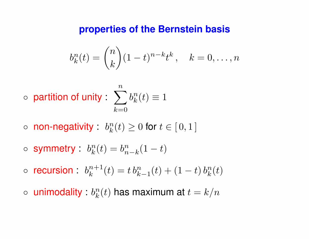
properties of the Bernstein basis
bnk(t) =(n
k
)(1− t)n−ktk , k = 0, . . . , n
◦ partition of unity :n∑k=0
bnk(t) ≡ 1
◦ non-negativity : bnk(t) ≥ 0 for t ∈ [ 0, 1 ]
◦ symmetry : bnk(t) = bnn−k(1− t)
◦ recursion : bn+1k (t) = t bnk−1(t) + (1− t) bnk(t)
◦ unimodality : bnk(t) has maximum at t = k/n
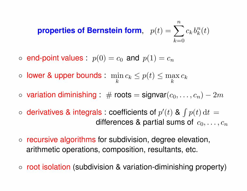
properties of Bernstein form, p(t) =n∑k=0
ck bnk(t)
◦ end-point values : p(0) = c0 and p(1) = cn
◦ lower & upper bounds : minkck ≤ p(t) ≤ max
kck
◦ variation diminishing : # roots = signvar(c0, . . . , cn)− 2m
◦ derivatives & integrals : coefficients of p′(t) &∫p(t) dt =
differences & partial sums of c0, . . . , cn
◦ recursive algorithms for subdivision, degree elevation,arithmetic operations, composition, resultants, etc.
◦ root isolation (subdivision & variation-diminishing property)
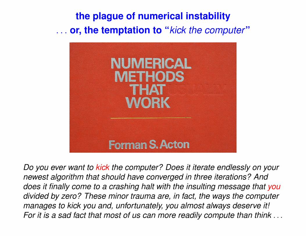
the plague of numerical instability. . . or, the temptation to “kick the computer”
Do you ever want to kick the computer? Does it iterate endlessly on yournewest algorithm that should have converged in three iterations? Anddoes it finally come to a crashing halt with the insulting message that youdivided by zero? These minor trauma are, in fact, the ways the computermanages to kick you and, unfortunately, you almost always deserve it!For it is a sad fact that most of us can more readily compute than think . . .
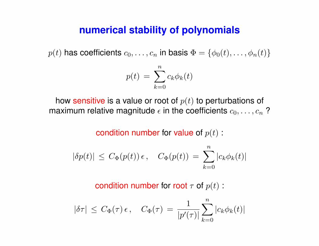
numerical stability of polynomials
p(t) has coefficients c0, . . . , cn in basis Φ = {φ0(t), . . . , φn(t)}
p(t) =n∑k=0
ckφk(t)
how sensitive is a value or root of p(t) to perturbations ofmaximum relative magnitude ε in the coefficients c0, . . . , cn ?
condition number for value of p(t) :
|δp(t)| ≤ CΦ(p(t)) ε , CΦ(p(t)) =n∑k=0
|ckφk(t)|
condition number for root τ of p(t) :
|δτ | ≤ CΦ(τ) ε , CΦ(τ) =1
|p′(τ)|
n∑k=0
|ckφk(t)|
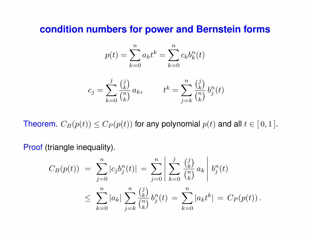
condition numbers for power and Bernstein forms
p(t) =n∑k=0
aktk =
n∑k=0
ckbnk(t)
cj =j∑
k=0
(jk
)(nk
) ak, tk =n∑j=k
(jk
)(nk
) bnj (t)
Theorem. CB(p(t)) ≤ CP (p(t)) for any polynomial p(t) and all t ∈ [ 0, 1 ].
Proof (triangle inequality).
CB(p(t)) =n∑j=0
|cjbnj (t)| =n∑j=0
∣∣∣∣∣j∑
k=0
(jk
)(nk
) ak∣∣∣∣∣ bnj (t)
≤n∑k=0
|ak|n∑j=k
(jk
)(nk
) bnj (t) =n∑k=0
|aktk| = CP (p(t)) .
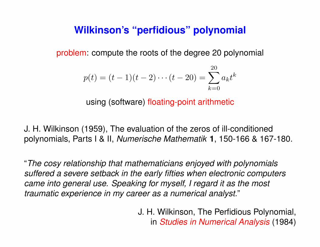
Wilkinson’s “perfidious” polynomial
problem: compute the roots of the degree 20 polynomial
p(t) = (t− 1)(t− 2) · · · (t− 20) =20∑k=0
aktk
using (software) floating-point arithmetic
J. H. Wilkinson (1959), The evaluation of the zeros of ill-conditionedpolynomials, Parts I & II, Numerische Mathematik 1, 150-166 & 167-180.
“The cosy relationship that mathematicians enjoyed with polynomialssuffered a severe setback in the early fifties when electronic computerscame into general use. Speaking for myself, I regard it as the mosttraumatic experience in my career as a numerical analyst.”
J. H. Wilkinson, The Perfidious Polynomial,in Studies in Numerical Analysis (1984)
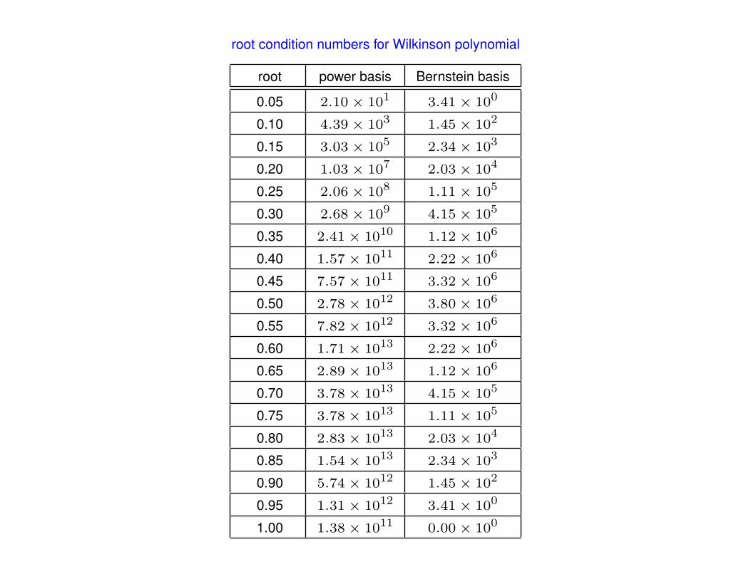
root condition numbers for Wilkinson polynomial
root power basis Bernstein basis
0.05 2.10× 101 3.41× 100
0.10 4.39× 10³ 1.45× 10²
0.15 3.03× 10⁵ 2.34× 10³
0.20 1.03× 10⁷ 2.03× 10⁴
0.25 2.06× 10⁸ 1.11× 10⁵
0.30 2.68× 10⁹ 4.15× 10⁵
0.35 2.41× 10¹⁰ 1.12× 10⁶
0.40 1.57× 10¹¹ 2.22× 10⁶
0.45 7.57× 10¹¹ 3.32× 10⁶
0.50 2.78× 10¹² 3.80× 10⁶
0.55 7.82× 10¹² 3.32× 10⁶
0.60 1.71× 10¹³ 2.22× 10⁶
0.65 2.89× 10¹³ 1.12× 10⁶
0.70 3.78× 10¹³ 4.15× 10⁵
0.75 3.78× 10¹³ 1.11× 10⁵
0.80 2.83× 10¹³ 2.03× 10⁴
0.85 1.54× 10¹³ 2.34× 10³
0.90 5.74× 10¹² 1.45× 10²
0.95 1.31× 10¹² 3.41× 100
1.00 1.38× 10¹¹ 0.00× 100
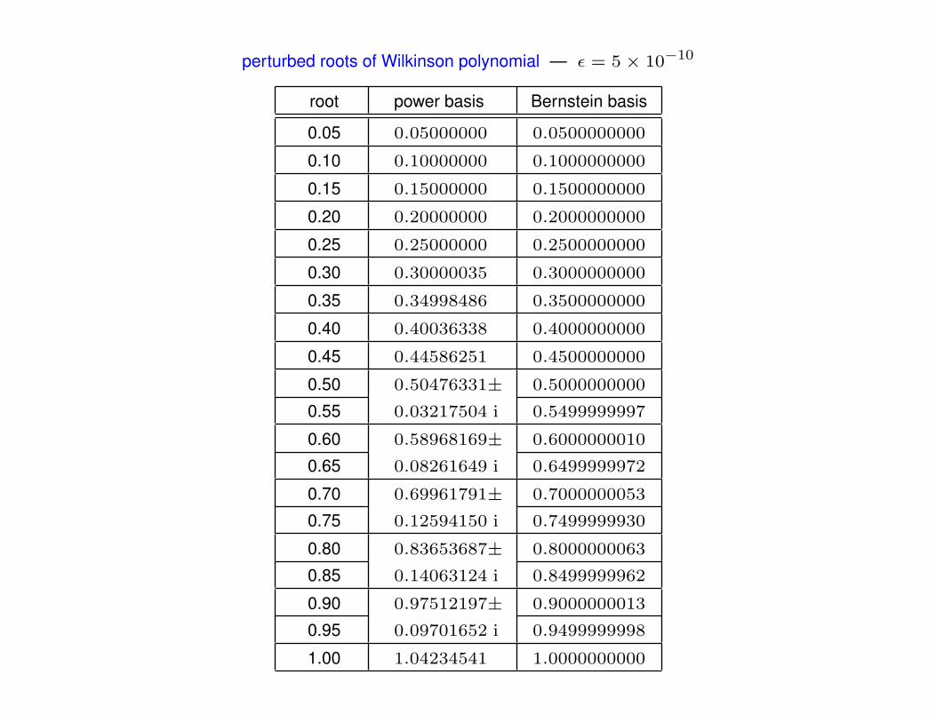
perturbed roots of Wilkinson polynomial — ε = 5× 10⁻¹⁰
root power basis Bernstein basis
0.05 0.05000000 0.0500000000
0.10 0.10000000 0.1000000000
0.15 0.15000000 0.1500000000
0.20 0.20000000 0.2000000000
0.25 0.25000000 0.2500000000
0.30 0.30000035 0.3000000000
0.35 0.34998486 0.3500000000
0.40 0.40036338 0.4000000000
0.45 0.44586251 0.4500000000
0.50 0.50476331± 0.5000000000
0.55 0.03217504 i 0.5499999997
0.60 0.58968169± 0.6000000010
0.65 0.08261649 i 0.6499999972
0.70 0.69961791± 0.7000000053
0.75 0.12594150 i 0.7499999930
0.80 0.83653687± 0.8000000063
0.85 0.14063124 i 0.8499999962
0.90 0.97512197± 0.9000000013
0.95 0.09701652 i 0.9499999998
1.00 1.04234541 1.0000000000
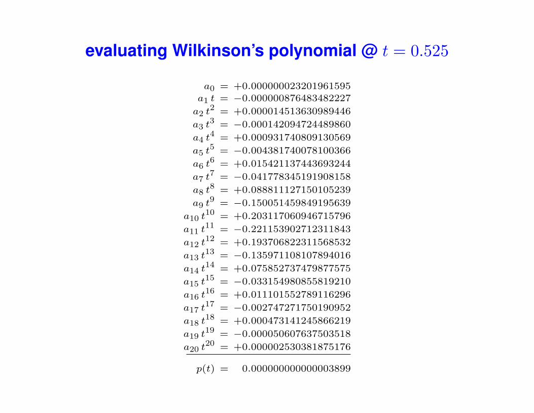
evaluating Wilkinson’s polynomial @ t = 0.525
a0 = +0.000000023201961595a1 t = −0.000000876483482227
a2 t2 = +0.000014513630989446
a3 t3 = −0.000142094724489860
a4 t4 = +0.000931740809130569
a5 t5 = −0.004381740078100366
a6 t6 = +0.015421137443693244
a7 t7 = −0.041778345191908158
a8 t8 = +0.088811127150105239
a9 t9 = −0.150051459849195639
a10 t10 = +0.203117060946715796
a11 t11 = −0.221153902712311843
a12 t12 = +0.193706822311568532
a13 t13 = −0.135971108107894016
a14 t14 = +0.075852737479877575
a15 t15 = −0.033154980855819210
a16 t16 = +0.011101552789116296
a17 t17 = −0.002747271750190952
a18 t18 = +0.000473141245866219
a19 t19 = −0.000050607637503518
a20 t20 = +0.000002530381875176
p(t) = 0.000000000000003899
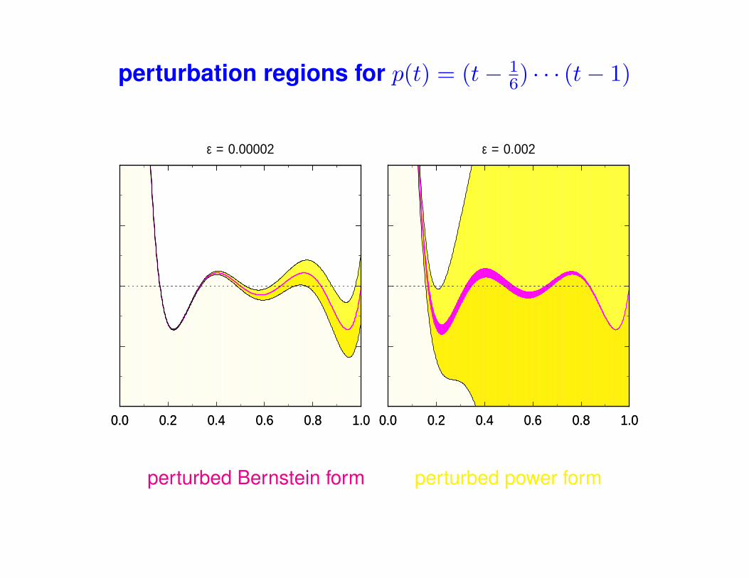
perturbation regions for p(t) = (t− 16) · · · (t− 1)
0.0 0.2 0.4 0.6 0.8 1.00.0 0.2 0.4 0.6 0.8 1.0
ε = 0.00002
0.0 0.2 0.4 0.6 0.8 1.00.0 0.2 0.4 0.6 0.8 1.0
ε = 0.002
perturbed Bernstein form perturbed power form
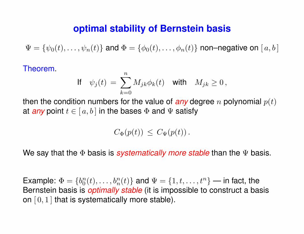
optimal stability of Bernstein basis
Ψ = {ψ0(t), . . . , ψn(t)} and Φ = {φ0(t), . . . , φn(t)} non–negative on [ a, b ]
Theorem.
If ψj(t) =n∑k=0
Mjkφk(t) with Mjk ≥ 0 ,
then the condition numbers for the value of any degree n polynomial p(t)at any point t ∈ [ a, b ] in the bases Φ and Ψ satisfy
CΦ(p(t)) ≤ CΨ(p(t)) .
We say that the Φ basis is systematically more stable than the Ψ basis.
Example: Φ = {bn0 (t), . . . , bnn(t)} and Ψ = {1, t, . . . , tn}— in fact, theBernstein basis is optimally stable (it is impossible to construct a basison [ 0, 1 ] that is systematically more stable).
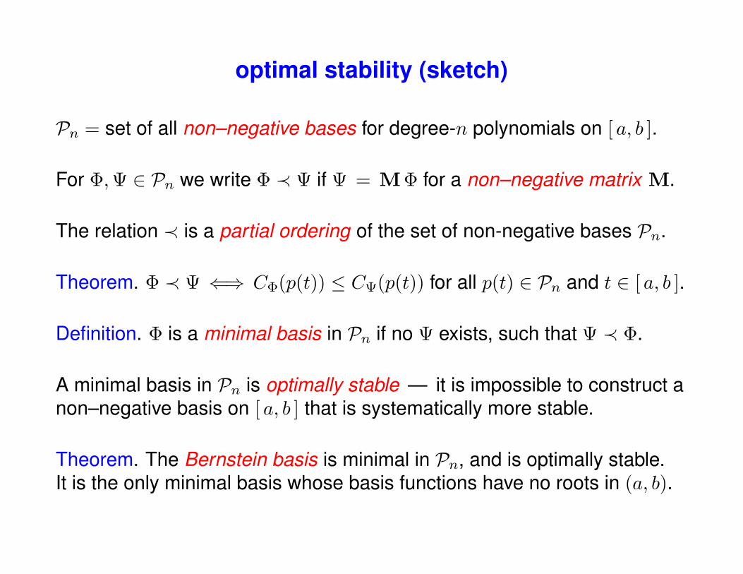
optimal stability (sketch)
Pn = set of all non–negative bases for degree-n polynomials on [ a, b ].
For Φ,Ψ ∈ Pn we write Φ ≺ Ψ if Ψ = M Φ for a non–negative matrix M.
The relation ≺ is a partial ordering of the set of non-negative bases Pn.
Theorem. Φ ≺ Ψ ⇐⇒ CΦ(p(t)) ≤ CΨ(p(t)) for all p(t) ∈ Pn and t ∈ [ a, b ].
Definition. Φ is a minimal basis in Pn if no Ψ exists, such that Ψ ≺ Φ.
A minimal basis in Pn is optimally stable — it is impossible to construct anon–negative basis on [ a, b ] that is systematically more stable.
Theorem. The Bernstein basis is minimal in Pn, and is optimally stable.It is the only minimal basis whose basis functions have no roots in (a, b).
condition numbers can be “very large” !
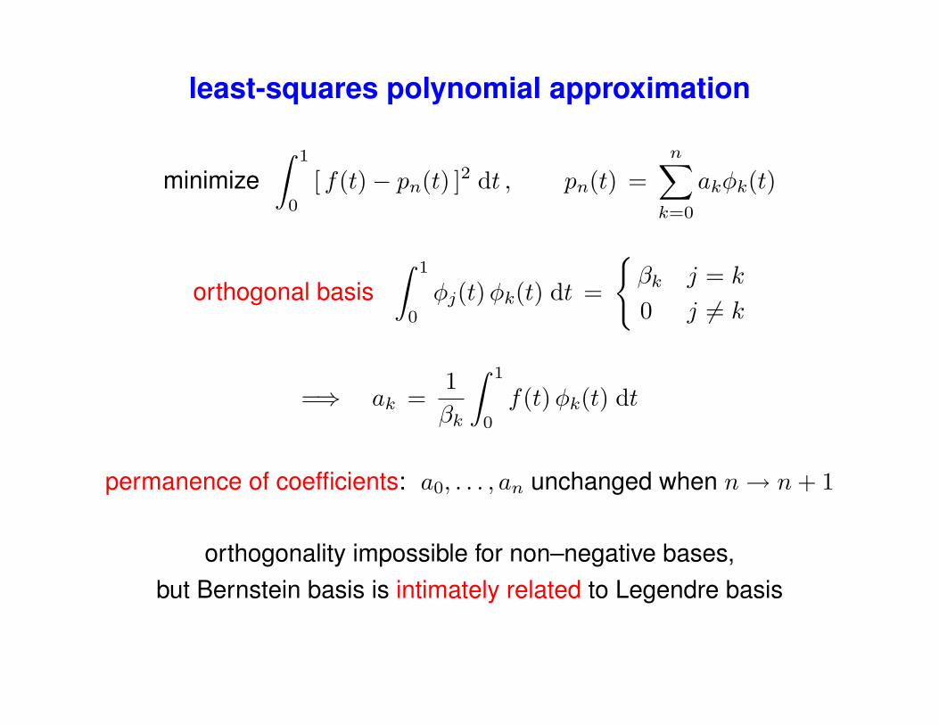
least-squares polynomial approximation
minimize∫ 1
0
[ f(t)− pn(t) ]2 dt , pn(t) =n∑k=0
akφk(t)
orthogonal basis∫ 1
0
φj(t)φk(t) dt =
{βk j = k
0 j 6= k
=⇒ ak =1βk
∫ 1
0
f(t)φk(t) dt
permanence of coefficients: a0, . . . , an unchanged when n→ n+ 1
orthogonality impossible for non–negative bases,but Bernstein basis is intimately related to Legendre basis
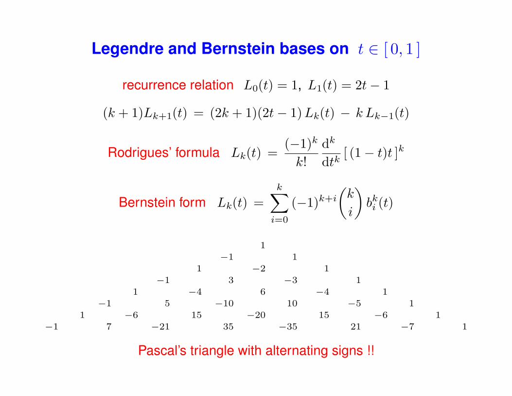
Legendre and Bernstein bases on t ∈ [ 0, 1 ]
recurrence relation L0(t) = 1, L1(t) = 2t− 1
(k + 1)Lk+1(t) = (2k + 1)(2t− 1)Lk(t) − k Lk−1(t)
Rodrigues’ formula Lk(t) =(−1)k
k!dk
dtk[ (1− t)t ]k
Bernstein form Lk(t) =k∑i=0
(−1)k+i
(k
i
)bki (t)
1−1 1
1 −2 1−1 3 −3 1
1 −4 6 −4 1−1 5 −10 10 −5 1
1 −6 15 −20 15 −6 1−1 7 −21 35 −35 21 −7 1
Pascal’s triangle with alternating signs !!
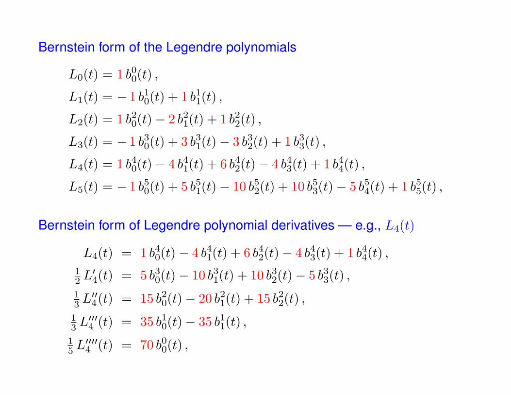
Bernstein form of the Legendre polynomials
L0(t) = 1 b00(t) ,
L1(t) = − 1 b10(t) + 1 b11(t) ,
L2(t) = 1 b20(t)− 2 b21(t) + 1 b22(t) ,
L3(t) = − 1 b30(t) + 3 b31(t)− 3 b32(t) + 1 b33(t) ,
L4(t) = 1 b40(t)− 4 b41(t) + 6 b42(t)− 4 b43(t) + 1 b44(t) ,
L5(t) = − 1 b50(t) + 5 b51(t)− 10 b52(t) + 10 b53(t)− 5 b54(t) + 1 b55(t) ,
Bernstein form of Legendre polynomial derivatives — e.g., L4(t)
L4(t) = 1 b40(t)− 4 b41(t) + 6 b42(t)− 4 b43(t) + 1 b44(t) ,12 L′4(t) = 5 b30(t)− 10 b31(t) + 10 b32(t)− 5 b33(t) ,
13 L′′4(t) = 15 b20(t)− 20 b21(t) + 15 b22(t) ,
13 L′′′4 (t) = 35 b10(t)− 35 b11(t) ,
15 L′′′′4 (t) = 70 b00(t) ,
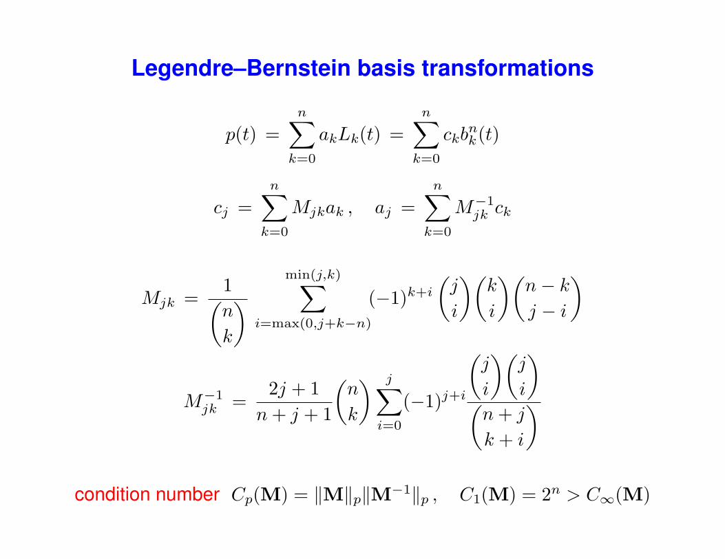
Legendre–Bernstein basis transformations
p(t) =n∑k=0
akLk(t) =n∑k=0
ckbnk(t)
cj =n∑k=0
Mjkak , aj =n∑k=0
M−1jk ck
Mjk =1(n
k
) min(j,k)∑i=max(0,j+k−n)
(−1)k+i
(j
i
)(k
i
)(n− kj − i
)
M−1jk =
2j + 1n+ j + 1
(n
k
) j∑i=0
(−1)j+i
(j
i
)(j
i
)(n+ j
k + i
)
condition number Cp(M) = ‖M‖p‖M−1‖p , C1(M) = 2n > C∞(M)
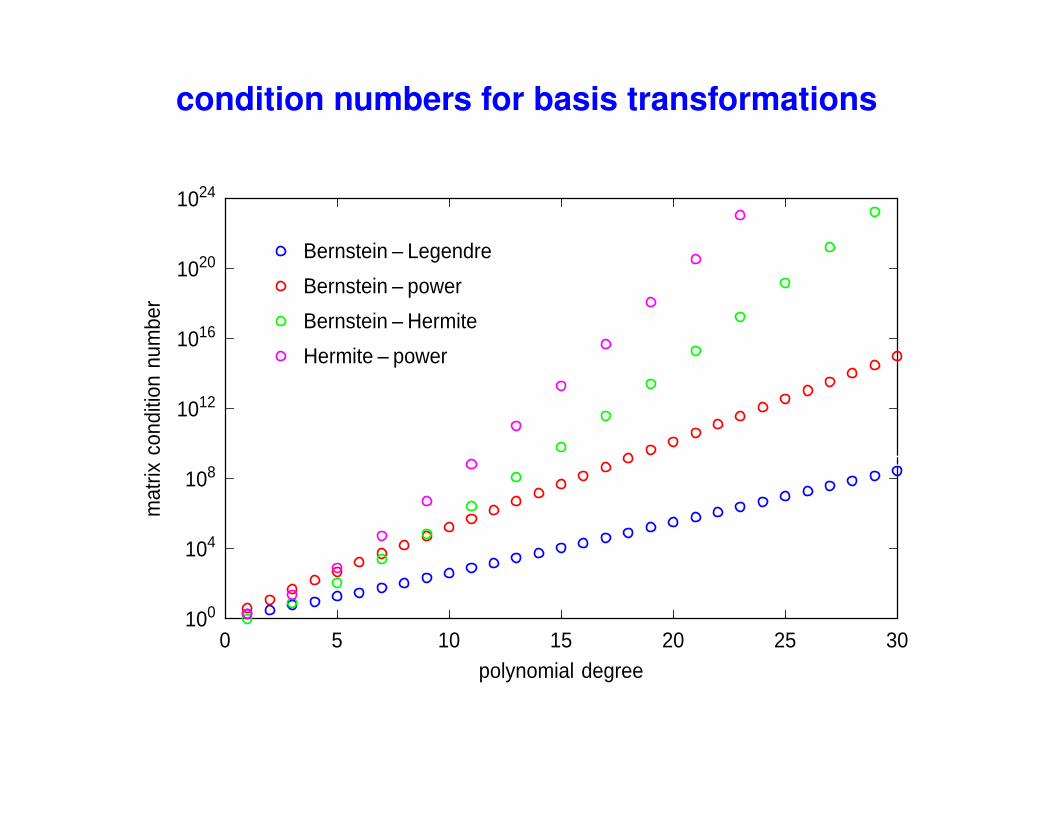
condition numbers for basis transformations
100
104
108
1012
1016
1020
1024
0 5 10 15 20 25 30polynomial degree
mat
rix c
ondi
tion
num
ber
Bernstein – Legendre
Bernstein – power
Bernstein – Hermite
Hermite – power
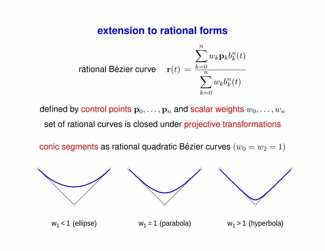
extension to rational forms
rational Bezier curve r(t) =
n∑k=0
wkpkbnk(t)
n∑k=0
wkbnk(t)
defined by control points p0, . . . ,pn and scalar weights w0, . . . , wn
set of rational curves is closed under projective transformations
conic segments as rational quadratic Bezier curves (w0 = w2 = 1)
w1 = 1 (parabola)w1 < 1 (ellipse) w1 > 1 (hyperbola)
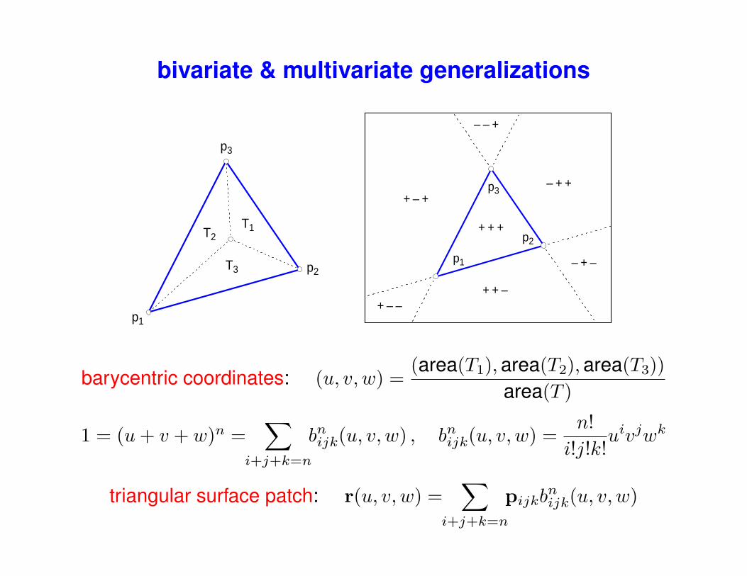
bivariate & multivariate generalizations
T3
T1T2
p1
p2
p3
p1
p2
p3
+ + +
– – +
– + +
– + –
+ + –+ – –
+ – +
barycentric coordinates: (u, v, w) =(area(T1),area(T2),area(T3))
area(T )
1 = (u+ v + w)n =∑
i+j+k=n
bnijk(u, v, w) , bnijk(u, v, w) =n!
i!j!k!uivjwk
triangular surface patch: r(u, v, w) =∑
i+j+k=n
pijkbnijk(u, v, w)
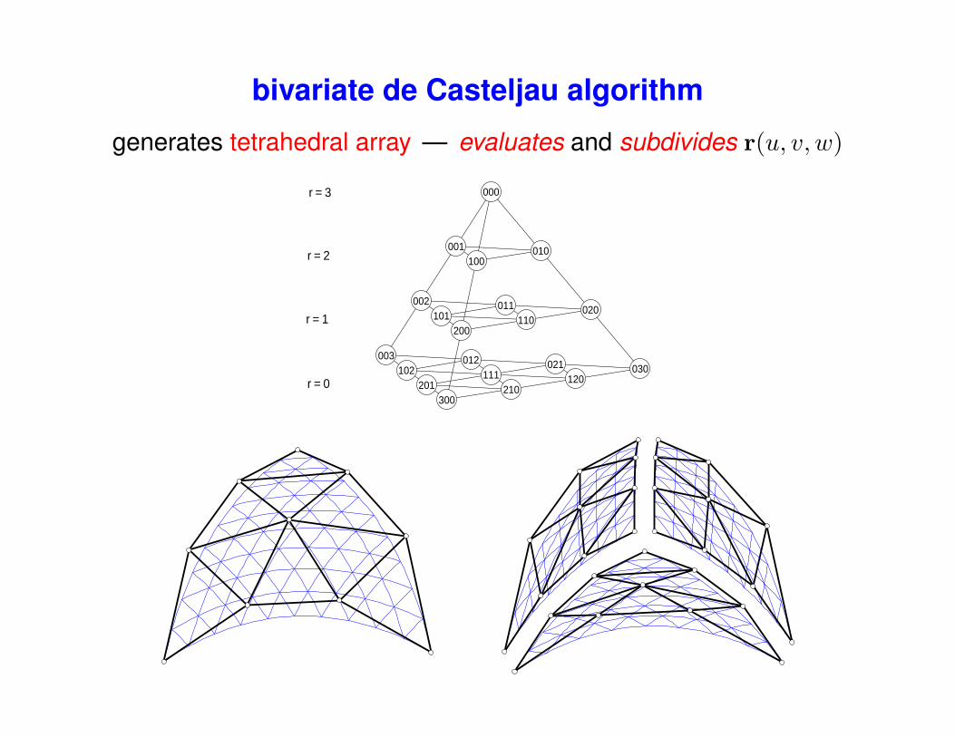
bivariate de Casteljau algorithm
generates tetrahedral array — evaluates and subdivides r(u, v, w)
003 012 021 030102 111 120201 210300
002 011 020101 110200
001 010100
000
r = 0
r = 1
r = 2
r = 3
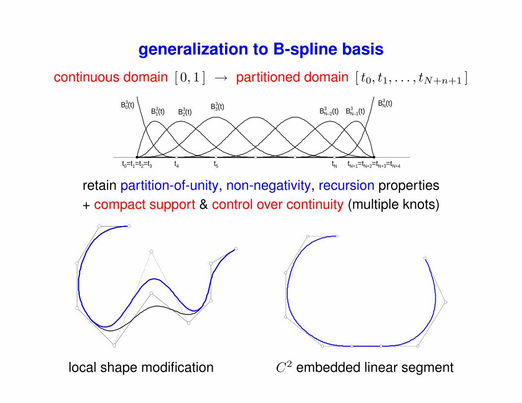
generalization to B-spline basis
continuous domain [ 0, 1 ] → partitioned domain [ t0, t1, . . . , tN+n+1 ]
t0=t1=t2=t3 t4 t5 tN tN+1=tN+2=tN+3=tN+4
B30(t)
B31(t) B3
2(t)B3
3(t) B3N–2(t) B3
N–1(t)B3
N(t)
retain partition-of-unity, non-negativity, recursion properties+ compact support & control over continuity (multiple knots)
local shape modification C2 embedded linear segment
scientific computing applications
◦ real solutions of systems of algebraic equations; identifying extremaor bounds on constrained or unconstrained polynomial functions in oneor several variables (optimization) using Bernstein basis properties
◦ robust stability of dynamic systems with uncertain physical parameters(Kharitonov generalization of Routh-Hurwitz criterion)
◦ definition of barycentric coordinates and “partition-of-unity” polynomialbasis functions over general polygon or polytope domains for use in thefinite-element and meshless analysis methods
◦ modelling of inter-molecular potential energy surfaces; design offilters for signal processing applications; inputs to neurofuzzy networksmodelling non-linear dynamical systems; reconstruction of 3D modelsand calibration of optical range sensors
closure
◦ 100 years have elapsed since introduction of Bernstein basis
◦ Bernstein form was limited to theory, rather than practice,∗
of polynomial approximation for ∼ 50 years after its introduction
◦ applications in design, rather than approximation, pioneered∼ 50 years ago by de Casteljau and Bezier
◦ now universally adopted as a fundamental representation forcomputer-aided geometric design applications
◦ “optimally stable” basis for polynomials defined over finite domains
◦ Bernstein basis intimately related to Legendre orthogonal basis
◦ increasing adoption in diverse scientific computing applications
“In theory, there is no difference between theory and practice. In practice, there is.” . . . Yogi Berra