The geometry of knot complements

Abhijit Champanerkar

Department of Mathematics,

College of Staten Island & The Graduate Center, CUNY

Mathematics Colloquium

Medgar Evers College

What is a knot ?

A knot is a (smooth) embedding of the circle S1 in S3. Similarly, a

link of k-components is a (smooth) embedding of a disjoint union

of k circles in S3.

Figure-8 knot Whitehead link Borromean rings

Two knots are equivalent if there is continuous deformation

(ambient isotopy) of S3 taking one to the other.

Goals: Find a practical method to classify knots upto equivalence.

Knot Diagrams

A common way to describe a knot is using a planar projection of

the knot which is a 4-valent planar graph indicating the over and

under crossings called a knot diagram.

A given knot has many

different diagrams.

Two knot diagrams represent

the same knot if and only if

they are related by a sequence

of three kinds of moves on

the diagram called the

Reidemeister moves.

Origins of Knot theory

In 1867, Lord Kelvin conjectured that atoms were knotted tubes of

ether and the variety of knots were thought to mirror the variety of

chemical elements. This theory inspired the celebrated Scottish

physicist Peter Tait to undertake an extensive study and tabulation

of knots (in collaboration with C. N. Little).

Tait enumerated knots using their

diagrammatic complexity called the

crossing number of a knot, defined as

the minimal number of crossings over

all knot diagrams.

However, there is no ether ! So physicists lost interest in knot

theory, till about 1980s.

Knot table by crossing number

Knot invariants

A knot invariant is a “quantity” that is equal for equivalent knots

and hence can be used to tell knots apart.

Knot invariants appear in two basic flavors:

Topological invariants arising

from the topology of the knot

complement S3 − K e.g.

Fundamental group.

Diagrammatic invariants arising

from the combinatorics of the

knot diagrams e.g. crossing

number.

Topological knot invariants

Let N(K ) denote a tubular neighbourhood of the knot K . Then

M = S3 −◦

N(K ) is a 3-manifold with a torus boundary. Examples

of basic topological invariants:

I Alexander polynomial (1927) describes the homology of the

infinite cyclic cover as Z[t±]-module.

I Invariants from Seifert surfaces

(1934) like knot genus, signature,

determinant etc.

I Representation of π1(S3 − K ) into finite and infinite groups.

I Knot Heegaard Floer homology (Ozsvath-Szabo-Rasmussen,

2003) categorified the Alexander polynomial.

Diagrammatic knot invariants

Any quantity which is invariant under the three Reidemeister

moves is a knot invariant. Examples of diagrammatic invariants:

I Tricolorability, Fox n-colorings

(Fox, 1956).

I Jones polynomial (1984), discovered via

representations of braid groups, led to

many new quantum invariants, which

can be computed diagrammatically, e.g.

Kauffman bracket (1987).

I Using Jones polynomial and relations to graph theory, Tait

conjectures from 100 years were resolved (1987).

I Khovanov homology (1999) categorified the Jones polynomial.

Knots and 3-manifolds

Since the boundary of M = S3 −◦

N(K ) is a torus, we can attach a

solid torus by choosing a curve (p, q) on ∂M which becomes

meridian. The resulting closed 3-manifold is called (p, q)-Dehn

filling of M. In general the process of drilling a simple closed curve

and filling it with a solid torus is called Dehn surgery.

M

V

Theorem (Lickorish-Wallace, 1960)

Any closed, orientable, connected 3-manifold can be obtained by

Dehn surgery on a link in S3.

Now enters geometry ....

In 1980s, William Thurstons seminal work established a strong

connection between hyperbolic geometry and knot theory, namely

that most knot complements are hyperbolic. Thurston introduced

tools from hyperbolic geometry to study knots that led to new

geometric invariants, especially hyperbolic volume.

Basic hyperbolic geometry I

I The Poincare half-space model of hyperbolic 3-space

H3 = {(x , y , t)|t > 0} with metric ds2 = dx2+dy2+dt2

t2. The

boundary of H3 is C ∪∞ called the sphere at infinity.

I Geodesic planes (H2) are vertical planes or upper hemispheres

of spheres orthogonal to the xy -plane (with centers on the

xy -plane).

I Geodesics are lines or half circles orthogonal to the xy -plane.

I Isom+(H3) = PSL(2,C) which acts as Mobius transforms on

C ∪∞ extending this action by isometries.

I The horizontal planes (t =constant) are scaled Euclidean

planes called horospheres.

Basic hyperbolic geometry II

Escher’s work using Poincare disc Crochet by Daina Taimina

Hyperbolic upper-half plane Hyperbolic upper-half space

Hyperbolic 3-manifolds

A 3-manifold M is said to be hyperbolic if it has a complete, finite

volume hyperbolic metric.

I π1(M) = Γ acts by covering translations as isometries and

hence has a discrete faithful representation in PSL(2,C).

I (Margulis 1978) If M is orientable and noncompact then

M =◦

M ′ where ∂M ′ = ∪T 2. Each end is of the form

T 2 × [0,∞) with each section is scaled Euclidean metric,

called a cusp.

I (Mostow-Prasad Rigidity, 1968) Hyperbolic structure on a

3-manifold is unique. This implies geometric invariants are

topological invariants !

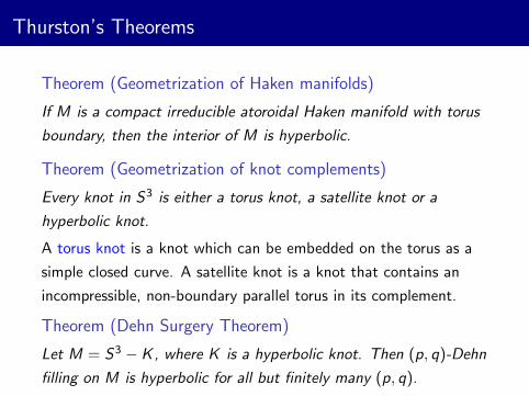
Thurston’s Theorems

Theorem (Geometrization of Haken manifolds)

If M is a compact irreducible atoroidal Haken manifold with torus

boundary, then the interior of M is hyperbolic.

Theorem (Geometrization of knot complements)

Every knot in S3 is either a torus knot, a satellite knot or a

hyperbolic knot.

A torus knot is a knot which can be embedded on the torus as a

simple closed curve. A satellite knot is a knot that contains an

incompressible, non-boundary parallel torus in its complement.

Theorem (Dehn Surgery Theorem)

Let M = S3 − K , where K is a hyperbolic knot. Then (p, q)-Dehn

filling on M is hyperbolic for all but finitely many (p, q).

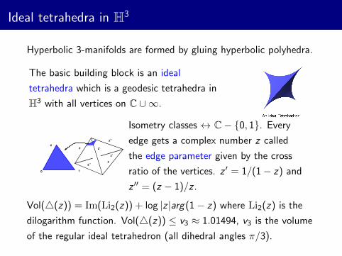
Ideal tetrahedra in H3

Hyperbolic 3-manifolds are formed by gluing hyperbolic polyhedra.

The basic building block is an ideal

tetrahedra which is a geodesic tetrahedra in

H3 with all vertices on C ∪∞.

0 1

zz z’

z’’

zz’’

z’

Isometry classes ↔ C− {0, 1}. Every

edge gets a complex number z called

the edge parameter given by the cross

ratio of the vertices. z ′ = 1/(1− z) and

z ′′ = (z − 1)/z .

Vol(4(z)) = Im(Li2(z)) + log |z |arg(1− z) where Li2(z) is the

dilogarithm function. Vol(4(z)) ≤ v3 ≈ 1.01494, v3 is the volume

of the regular ideal tetrahedron (all dihedral angles π/3).

Ideal triangulations

An ideal triangulation of a cusped (non-compact) hyperbolic

3-manifold M is a decompostion of M into ideal tetrahedra glued

along the faces with the vertices deleted.

Around every edge, the parameters multiply together to ±1

ensuring hyperbolicity around the edges. The completeness

condition gives a condition on every cusp torus giving a similar

equation in the edge parameters. These are called gluing and

completeness equations.

Thurston proved that the solution set to these equations is

discrete, the paramters are algebraic numbers and give the

complete hyperbolic structure on M. Vol(M) is a sum of volumes

of ideal tetrahedra.

Example: Figure-8 knot

1 2

3

4

3

3 4

4

1

1

2

2

11

2

23

34

4

B−

B+

More hyperbolic structures

I Hyperbolic structures on some link complements can be

described using circle packings and dual packings via the

Koebe-Andreev-Thurston circle packing theorem which relates

circle packings to triangulations of S2.

I Hyperbolic structures on fibered 3-manifolds i.e. surface

bundles can be obtained by using a psuedo-Anosov

monodromy. The first examples of hyperbolic 3-manifolds

were obtained as surface bundles by Jorgensen (1977).

I Hyperbolic 3-manifolds also arise as quotients of arithmetic

lattices in PSL(2,C) e.g. finite index subgroups of PSL(2,O),

where O is the ring of integers of some number field.

Computing hyperbolic structures

The program SnapPea by Jeff Weeks (1999) computes hyperbolic

structures and invariants on 3-manifolds and knots by triangulating

and solving gluing equations. It also includes census of hyperbolic

manifolds triangulated using at most 7 tetrahedra (4815 manifolds)

and census of low volume closed hyperbolic 3-manifolds.

SnapPy by Culler and

Dunfield is a modification of

SnapPea which uses python

interface. Snap by Goodman

uses SnapPea to compute

arithmetic invariants of

hyperbolic 3-manifolds.

Simplest hyperbolic knots

The geometric complexity is the minimum number of ideal

tetrahedra used to triangulate a hyperbolic knot complement. The

census of hyperbolic knots using this measure of complexity gives a

different view of the space of all knots e.g. many of the

geometrically simple knots have very high crossing numbers.

Hyperbolic knots with geometric complexity up to 6 tetrahedra

were found by Callahan-Dean-Weeks (1999), extended to 7

tetrahedra by Champanerkar-Kofman-Paterson (2004).

Tetrahedra 1 2 3 4 5 6 7 8

Knots 0 1 2 4 22 43 129 299

Simplest hyperbolic knots

Extending the census of simplest hyperbolic knots

Started as an REU project by Tim Mullen at CSI.

I Step 1 (Identifying the manifold): Starting with

Thistlethwaite’s census of cusped hyperbolic 3-manifolds

triangulated with 8 ideal tetrahedra (around 13000 manifolds,

included in SnapPy), find one-cusped manifolds which have a

Dehn filling homeomorphic to S3, checked using fundamental

group. Many cases involve using program testisom to simplify

presentation of fundamental group.

I Step 2 (Identify the knot): Find a knot diagram. SnapPy

can check isometry from diagram with manifold found in Step

1. Search through existing censuses of knots, generate

families and search through them. After the searches we were

left with around 20 knots.

Extending the census of simplest hyperbolic knots

I Step 3 (Kirby

Calculus): For knots

not resolved after Step

2, find a surgery

description of knots

and use Kirby calculus

to find knot diagram.

Example

Twisted torus knots

A torus knot is a knot which can be embedded on a torus as a

simple closed curve, and is parametrized by the slope p/q of the

lift of this curve to R2. Torus knot T (p, q) has p strands and q

overpasses.

A twisted torus knot T (p, q, r , s) is obtained by adding s

overpasses to the outermost r strands. Twisted torus knots

dominate the census of simplest hyperbolic knots.

T (9, 7) T (9, 7, 5, 3)

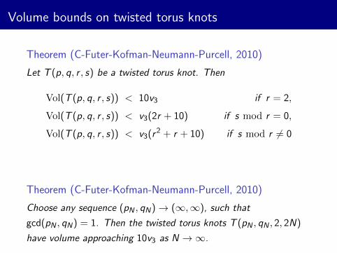
Volume bounds on twisted torus knots

Theorem (C-Futer-Kofman-Neumann-Purcell, 2010)

Let T (p, q, r , s) be a twisted torus knot. Then

Vol(T (p, q, r , s)) < 10v3 if r = 2,

Vol(T (p, q, r , s)) < v3(2r + 10) if s mod r = 0,

Vol(T (p, q, r , s)) < v3(r2 + r + 10) if s mod r 6= 0

Theorem (C-Futer-Kofman-Neumann-Purcell, 2010)

Choose any sequence (pN , qN)→ (∞,∞), such that

gcd(pN , qN) = 1. Then the twisted torus knots T (pN , qN , 2, 2N)

have volume approaching 10v3 as N →∞.

Open Questions and Conjectures

Its an interesting problem to understand how the topological,

diagrammatic and geometric invariants relate to one another.

I What is the topological or geometric interpretation of the

Jones polynomial or Khovanov homology ?

I How do the geometric invariants relate to the quantum

invariants ? Two big conjecture along these lines are the

Volume Conjecture (Kashaev, Murakami, Murakami, 2001)

and the AJ Conjecture (Garoufalidis, 2003).

I Understanding geometry of knot complements in terms of the

combinatorics of knot diagrams is an active area of research.

Some links

Abhijit’s Home page: http://www.math.csi.cuny.edu/abhijit/

KnotAtlas: http://katlas.math.toronto.edu/wiki/

SnapPy: http://www.math.uic.edu/ t3m/SnapPy/

KnotPlot: http://www.knotplot.com/

Thank you