Embed Size (px)
Citation preview
COMMENSURATORS OF CUSPED HYPERBOLIC MANIFOLDS
OLIVER GOODMAN, DAMIAN HEARD, AND CRAIG HODGSON
Abstract. This paper describes a general algorithm for finding the commen-
surator of a non-arithmetic hyperbolic manifold with cusps, and for decidingwhen two such manifolds are commensurable. The method is based on some
elementary observations regarding horosphere packings and canonical cell de-
compositions. For example, we use this to find the commensurators of allnon-arithmetic hyperbolic once-punctured torus bundles over the circle.
For hyperbolic 3-manifolds, the algorithm has been implemented using
Goodman’s computer program Snap. We use this to determine the commensu-rability classes of all cusped hyperbolic 3-manifolds triangulated using at most
7 ideal tetrahedra, and for the complements of hyperbolic knots and links with
up to 12 crossings.
1. Introduction
Two manifolds or orbifolds M and M ′ are commensurable if they admit a com-mon finite sheeted covering. For hyperbolic n-orbifolds, we can suppose thatM = Hn/Γ and M ′ = Hn/Γ′, with Γ and Γ′ discrete subgroups of Isom(Hn).In this paper, we assume that M and M ′ are of finite volume and of dimension atleast 3. Then, by Mostow-Prasad Rigidity, commensurability means that we canconjugate Γ by an isometry g such that gΓg−1 and Γ′ intersect in a subgroup offinite index in both groups.
Given that the classification of finite volume hyperbolic manifolds up to homeo-morphism appears to be hard, it seems sensible to attempt to subdivide the problemand start with a classification up to commensurability. Looked at in this way, wesee a remarkable dichotomy between the arithmetic and non-arithmetic cases. (See[23] for the definition of arithmetic hyperbolic manifolds.)
Define the commensurator of Γ to be the group
Comm(Γ) = {g ∈ Isom(Hn) | [Γ : Γ ∩ gΓg−1] <∞}.
Then Γ and Γ′ are commensurable if and only if Comm(Γ) and Comm(Γ′) are con-jugate. Geometrically, an element of the normalizer of Γ in Isom(Hn) represents asymmetry (i.e. isometry) of M = Hn/Γ. Similarly, an element of the commensura-tor represents an isometry between finite sheeted covers of M ; this gives a hiddensymmetry of M if it is not the lift of an isometry of M (see [27]).
It follows from deep work of Margulis [24] (see also [35]), that in dimension≥ 3, the commensurator Comm(Γ) is discrete if and only if Γ is not arithmetic.This means that the commensurability class of a non-arithmetic, cofinite volume,discrete group Γ is particularly simple, consisting only of conjugates of the finiteindex subgroups of Comm(Γ). In terms of orbifolds, it means that M and M ′ arecommensurable if and only if they cover a common quotient orbifold.
On the other hand, commensurability classes of arithmetic groups are “big”: wemay well have commensurable Γ and Γ′ such that the group generated by gΓg−1
and Γ′ is not discrete for any g.
This work was partially supported by grants from the Australian Research Council.
1
arX
iv:0
801.
4815
v1 [
mat
h.G
T]
31
Jan
2008
2 OLIVER GOODMAN, DAMIAN HEARD, AND CRAIG HODGSON
A hyperbolic n-orbifold is cusped if it is non-compact of finite volume. Thispaper describes a practical algorithm for determining when two cusped hyperbolicn-manifolds cover a common quotient, and for finding a smallest quotient. Fornon-arithmetic finite volume cusped hyperbolic n-manifolds of dimension n ≥ 3,this solves the commensurability problem.
Section 2 begins with some elementary observations about horoball packingsand canonical cell decompositions of a cusped hyperbolic manifold. This leadsto a characterization of the commensurator of a non-arithmetic cusped hyperbolicmanifold M as the maximal symmetry group of the tilings of Hn obtained by liftingcanonical cell decompositions of M . In Section 3, we use this to determine thecommensurators of non-arithmetic hyperbolic once-punctured torus bundles overthe circle.
Section 4 gives an algorithm for finding the isometry group of a tiling of Hn
arising from a cell decomposition of a hyperbolic manifold, and Sections 5 and 6describe methods for finding all possible canonical cell decompositions for a cuspedhyperbolic manifold. Section 7 contains some observations on commensurability ofcusps in hyperbolic 3-manifolds which can simplify the search for all canonical celldecompositions.
In 3-dimensions, each orientable hyperbolic orbifold has the form M = H3/Γ,where Γ is a discrete subgroup of PSL(2,C) = Isom+(H3). The invariant trace fieldk(Γ) ⊂ C is the field generated by the traces of the elements of Γ(2) = {γ2 | γ ∈ Γ}lifted to SL(2,C). This is a number field if M has finite volume (see [27], [29],[22]). The invariant quaternion algebra is the k(Γ) subalgebra of M2(C) generatedby Γ(2). These are useful and computable commensurability invariants (see [10],[23]).
For the arithmetic subgroups of Isom(H3), the invariant quaternion algebra is acomplete commensurability invariant. In fact for cusped arithmetic hyperbolic 3-orbifolds, the invariant trace field is an imaginary quadratic field and the quaternionalgebra is just the algebra of all 2×2 matrices with entries in the invariant trace field(see [23, Theorem 3.3.8]); so the invariant trace field is a complete commensurabilityinvariant. However most cusped hyperbolic 3-manifolds are non-arithmetic (cf. [6])so other methods are needed to determine commensurability.
Damian Heard and Oliver Goodman have implemented the algorithms describedin this paper for non-arithmetic hyperbolic 3-manifolds; these are incorporated inthe computer program Snap [16]. Using this we have determined the commensura-bility classes for all manifolds occurring in the Callahan-Hildebrand-Weeks census([19], [9]) of cusped hyperbolic manifolds with up to 7 tetrahedra, and for com-plements of hyperbolic knots and links up to 12 crossings, supplied by MorwenThistlethwaite (see [20]). These results are discussed in Section 8, while Section 9outlines the Dowker-Thistlethwaite notation used to describe links.
This work has uncovered interesting new examples of commensurable knot andlink complements (see Examples 2.1 and 2.2), and a new example of a knot withshape field properly contained in the invariant trace field (see Example 7.1). Theresults have also been used by Button [8] to study fibred and virtually fibred cuspedhyperbolic 3-manifolds.
For 1-cusped manifolds we note that “cusp density” (see Section 2) is a verygood invariant. We have found only a few examples of incommensurable 1-cuspedmanifolds which are not distinguished by cusp density (see Example 2.3).
There is also a “dumb” algorithm, based on volume bounds for hyperbolic orb-ifolds, which works for any (possibly closed) non-arithmetic hyperbolic 3-orbifold,but appears to be quite impractical. If M and M ′ cover Q with Vol(Q) > Cthen the degrees d, d′ of the coverings are bounded by D = bVol(M)/Cc and
COMMENSURATORS OF CUSPED HYPERBOLIC MANIFOLDS 3
D′ = bVol(M ′)/Cc, respectively. Then if M and M ′ are commensurable, theyadmit a common covering N of degree at most D′ over M and at most D overM ′. The best current estimate for C for orientable non-arithmetic 3-orbifolds is0.041 . . . from recent work of Marshall-Martin [25]. Since Vol(M) ≈ 2 is typical,we would have to find all coverings of M ′ of degree d′ ≤ 50. This means findingall conjugacy classes of transitive representations of π1(M ′) into S50, a group witharound 1064 elements!
Acknowledgements: We thank Ian Agol for pointing out a simplification to ourmethod of determining the commensurability of Euclidean tori, Gaven Martin forinformation on current volume bounds, and Walter Neumann for several interestingdiscussions on this work. We also thank Alan Reid, Genevieve Walsh, and thereferee for their helpful comments on the paper.
2. The Commensurability Criterion
We use the following terminology throughout this paper. A set of disjointhoroballs in Hn is called a horoball packing, and a cusp neighbourhood in a hy-perbolic n-orbifold is one which lifts to such a horoball packing.
Lemma 2.1. The symmetry group of a horoball packing in Hn is discrete wheneverthe totally geodesic subspace spanned by their ideal points has dimension at leastn− 1.
Proof. Let {gi} be a sequence of symmetries of the packing converging to the iden-tity. Choose horoballs B1, . . . , Bn whose ideal points span a totally geodesic sub-space H of dimension n−1. For i sufficiently large, we can assume that gi(Bk) = Bkfor k = 1, . . . , n. But this implies that these gi fix H pointwise. Since the only suchisometries are the identity, and reflection in H, the sequence must be eventuallyconstant. �
Lemma 2.2. Let M = Hn/Γ be a finite volume cusped hyperbolic orbifold. The setof parabolic fixed points of Γ spans Hn.
Proof. The set of parabolic fixed points is dense in the limit set of Γ which equalsthe whole of the sphere at infinity. �
Lemma 2.3. Let M , M ′ be finite volume cusped hyperbolic orbifolds. Then M andM ′ cover a common orbifold Q if and only if they admit choices of cusp neighbour-hoods lifting to isometric horoball packings.
Proof. If M and M ′ cover Q, choose cusp neighbourhoods in Q and lift to M andM ′. These all lift to the same horoball packing in Hn, namely the horoball packingdetermined by our choice of cusp neighbourhoods in Q. Conversely, both M andM ′ cover the quotient of Hn by the group of symmetries of their common horoballpacking which, by Lemmas 2.1 and 2.2, is discrete. �
We can define the cusp density of a 1-cusped hyperbolic orbifold M as follows.SinceM has only one cusp it has a unique maximal (embedded) cusp neighbourhoodU . The cusp density of M is Vol(U)/Vol(M). Since the cusp density of any orbifoldcovered by M is the same, it is a commensurability invariant of orbifolds withdiscrete commensurator.
Choosing a full set of disjoint cusp neighbourhoods in a non-compact finite vol-ume hyperbolic n-manifold M determines a “Ford spine.” This is the cell complexgiven by the set of points in M equidistant from the cusp neighbourhoods in twoor more directions. Cells of dimension n − k contain points equidistant from thecusp neighbourhoods in k+1 independent directions (k = 1, . . . , n). This spine can
4 OLIVER GOODMAN, DAMIAN HEARD, AND CRAIG HODGSON
also be seen intuitively as the “bumping locus” of the cusp neighbourhoods: blowup the cusp neighbourhoods until they press against each other and flatten.
Dual to the Ford spine is a decomposition of M into ideal polytopes, genericallysimplices. The ideal cell dual to a given 0-cell of the Ford spine lifts to the con-vex hull in Hn of the set of ideal points determined by the equidistant directions.We call the cell decompositions that arise in this way canonical.1 For a 1-cuspedmanifold the canonical cell decomposition is unique. It is shown in [4] that a finitevolume hyperbolic manifold with multiple cusps admits finitely many canonical celldecompositions.
Theorem 2.4. Cusped hyperbolic n-manifolds M and M ′ cover a common orbifoldif and only if they admit canonical ideal cell decompositions lifting to isometrictilings of Hn.
Proof. If M and M ′ cover Q, choose cusp neighbourhoods in Q and lift them toM , M ′ and Hn. Constructing the Ford spine and cell decomposition in Hn clearlyyields the lifts of those entities from both M and M ′ corresponding to our choiceof cusp neighbourhoods.
Conversely, observe that the symmetry group of the common tiling gives anorbifold which is a quotient of both manifolds. �
Remark 2.5. We can omit the word ‘canonical’ in the above theorem. The proofis unchanged.
The previous theorem gives the following characterization of the commensurator.
Theorem 2.6. Let M = Hn/Γ be a finite volume cusped hyperbolic n-manifoldwith discrete commensurator. Then Comm(Γ) is the maximal symmetry group ofthe tilings of Hn obtained by lifting canonical cell decompositions of M ; it containsall such symmetry groups.
For manifolds with discrete commensurator, we can now define a truly canon-ical ideal cell decomposition as follows. Find Comm(Γ) as in the above theorem.Choose equal volume cusp neighbourhoods in Hn/Comm(Γ). Lift them to M andtake the resulting canonical cell decomposition of M . Two such manifolds are com-mensurable if and only if their truly canonical cell decompositions give isometrictilings of Hn.
Choosing maximal cusp neighbourhoods in Hn/Comm(Γ) also gives a canonicalversion of cusp density for multi-cusped manifolds.
Theorem 2.6 is the basis for the algorithms described in this paper. Canoni-cal cell decompositions can be computed by the algorithms of Weeks described in[33] and implemented in SnapPea [34]. In Section 4 below we give an algorithmfor finding the isometry groups of the corresponding tilings of Hn. Combiningthis with Theorem 2.6 gives an algorithm for finding commensurators of 1-cuspednon-arithmetic hyperbolic n-manifolds. In Sections 5 and 6 we extend this algo-rithm to multi-cusped manifolds, by describing methods for finding all canonicalcell decompositions.
For hyperbolic 3-manifolds, these algorithms have been implemented by Heardand Goodman. (These are incorporated in “find commensurator” and relatedcommands in the program Snap [16]). We conclude this section with some examplesdiscovered during this work.
1The term is not really ideal since, for manifolds with multiple cusps, there are generallymultiple canonical cell decompositions depending on the choice of cusp neighbourhoods.

COMMENSURATORS OF CUSPED HYPERBOLIC MANIFOLDS 5
2.1. Example: a 5-link chain and friends. The following five links have com-mensurable complements, as shown using our computer program. In the first threecases at least it is possible to ‘see’ this commensurability.
The first of these is the 5-link chain C5. Thurston [32, Chapter 6] explains how toobtain a fundamental region for the hyperbolic k-link chain complements: we spaneach link of the chain by a disk in the obvious manner. The complement of theunion of these five disks is then a solid torus. Once the link is deleted, the disks andtheir arcs of intersection divide the boundary of the solid torus into ideal squaresA,B,C,D,E as shown, with cusps labelled a, b, c, d, e.
A
A
B
B
C
C
D
D
E
EC D E A B C D
A B C D E A BE A
D E
a b c d e a
e a b c d e
d e a b c d
A hyperbolic structure is given by taking two regular pentagonal drums withideal vertices and adjusting their heights to obtain (ideal) square faces. Glue twodrums together as shown, identify the top with the bottom via a 4π
5 rotation, andglue faces as indicated. Edges are then identified in 4’s, two horizontal with twovertical. It is easy to check that the sum of dihedral angles around each edge is 2πso this gives a hyperbolic structure, since the angle sum is π at each ideal vertex ofa drum.
CD
AB
E
EA
BC
D
ab
c
d
e ea
b
c
d de
a
b
c
6 OLIVER GOODMAN, DAMIAN HEARD, AND CRAIG HODGSON
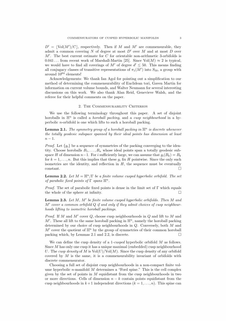
It is clear from the symmetry of the picture that the drums are cells in the canon-ical cell decomposition obtained by choosing equal area cusp cross sections. Weremark that Neumann-Reid show that this link complement is non-arithmetic in[27, Section 5].
Now change the 5-link chain by cutting along the shown disk, applying a halftwist, and re-gluing to obtain our second link. In the complement, this surgeryintroduces a half turn into the gluing between the A-faces. Edges are still identifiedin 4’s, two horizontal with two vertical, but there are now only four cusps.
CD
AB
E
E A
BC
D
ab
c
d
b ba
b
c
d db
a
b
c
If we repeat the process on the second disk shown we obtain the third link. Againthis corresponds to changing the gluing pattern on our two drums.
Since these link complements are non-arithmetic, the tiling of H3 by pentagonaldrums covers some canonical cell decomposition of each one. Since their volumesare the same, each one decomposes into two pentagonal drums. It should thereforebe possible, in each case, to find 5 ideal squares meeting at order 4 edges, cuttingthe complement into one or two solid tori. We leave this as a challenge for thereader.
2.2. Example: commensurable knot complements. Commensurable knot com-plements seem to be rather rare. Previously known examples include the Rubinstein-Aitchison dodecahedral knots [3] and examples due to a construction of Gonzales-Acuna and Whitten [13] giving knot complements covering other knot complements.For example, the−2, 3, 7 pretzel knot has 18/1 and 19/1 surgeries giving lens spaces.Taking the universal covers of these lens spaces gives new hyperbolic knots in S3
whose complements are 18- and 19-fold cylic covers of the (−2, 3, 7)–pretzel com-plement.
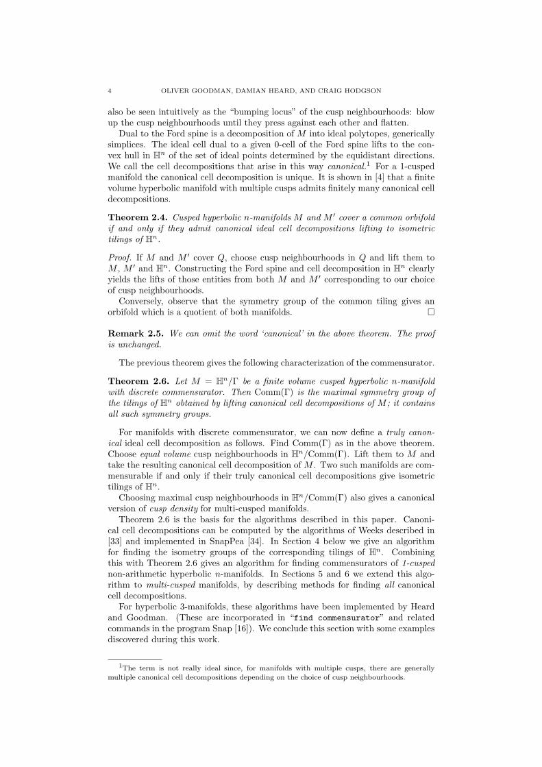
Our program finds a pair of knots “9n6” and “12n642”, having 9 and 12 crossingsrespectively, whose complements are commensurable with volumes in the ratio 3 : 4.Walter Neumann has pointed out that these knots belong to a very pretty familyof knots: take a band of k repeats of a trefoil with the ends given m half twistsbefore putting them together. E.g. (k,m) = (3, 2):
COMMENSURATORS OF CUSPED HYPERBOLIC MANIFOLDS 7
The half-twists are put in so as to undo some of the crossings of the trefoils (allowingthe above projection to be rearranged so as to have 9 crossings). The pair of knotsfound by our program correspond to (k,m) = (3, 2) and (4, 1).
To see that these knots have commensurable complements we find a commonquotient orbifold. In each case this is the quotient of the knot complement by itssymmetry group; these are dihedral groups of order 12 and order 16 respectively.
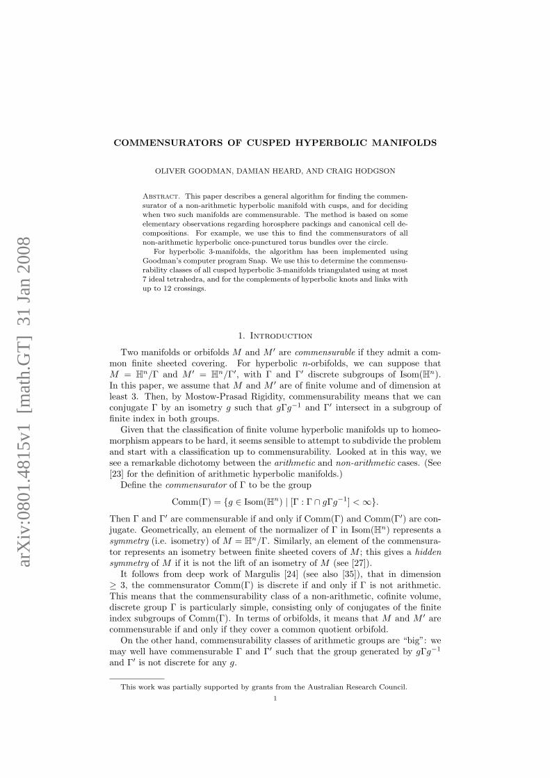
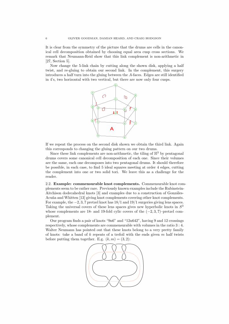
The picture of 9n6 above shows an obvious axis of 2-fold symmetry; below left isthe quotient, which is the complement of a knot in the orbifold S3 with singular setan unknot labelled 2. By pulling the knot straight, we see that this is an orbifoldwhose underlying space is a solid torus with knotted singular locus.
2 2
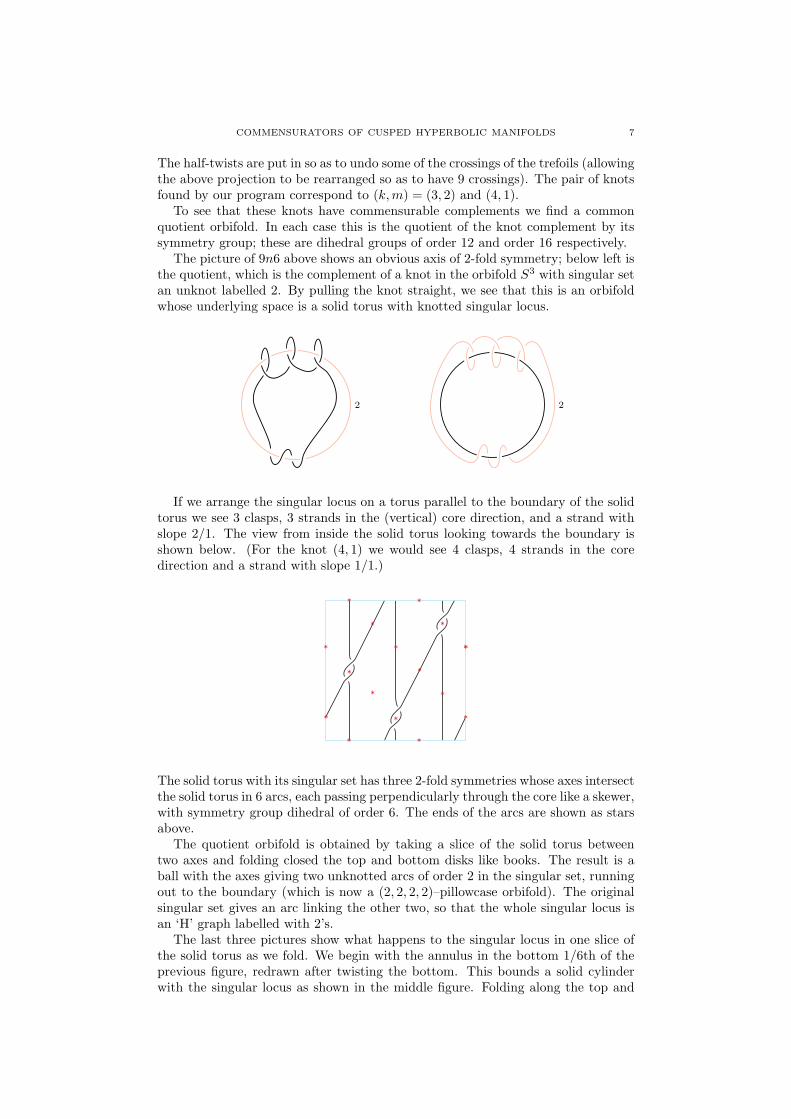
If we arrange the singular locus on a torus parallel to the boundary of the solidtorus we see 3 clasps, 3 strands in the (vertical) core direction, and a strand withslope 2/1. The view from inside the solid torus looking towards the boundary isshown below. (For the knot (4, 1) we would see 4 clasps, 4 strands in the coredirection and a strand with slope 1/1.)
*
*
*
*
*
*
*
* *
*
*
*
**
*
*
*
The solid torus with its singular set has three 2-fold symmetries whose axes intersectthe solid torus in 6 arcs, each passing perpendicularly through the core like a skewer,with symmetry group dihedral of order 6. The ends of the arcs are shown as starsabove.
The quotient orbifold is obtained by taking a slice of the solid torus betweentwo axes and folding closed the top and bottom disks like books. The result is aball with the axes giving two unknotted arcs of order 2 in the singular set, runningout to the boundary (which is now a (2, 2, 2, 2)–pillowcase orbifold). The originalsingular set gives an arc linking the other two, so that the whole singular locus isan ‘H’ graph labelled with 2’s.
The last three pictures show what happens to the singular locus in one slice ofthe solid torus as we fold. We begin with the annulus in the bottom 1/6th of theprevious figure, redrawn after twisting the bottom. This bounds a solid cylinderwith the singular locus as shown in the middle figure. Folding along the top and
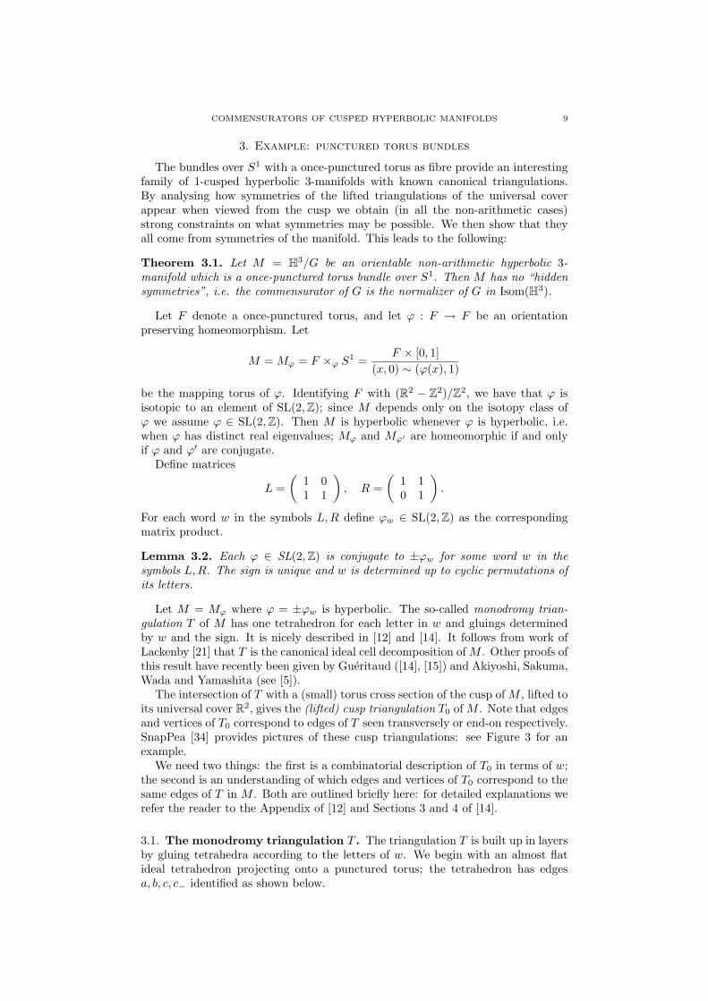
8 OLIVER GOODMAN, DAMIAN HEARD, AND CRAIG HODGSON
bottom (and expanding the region slightly) gives the final result.
*
* *
* *
*
We leave it to the reader to draw similar pictures for the knot with (k,m) = (4, 1)and verify that the result is indeed the same orbifold. Alternatively, Orb [18] orSnapPea [34] can be used to verify that the appropriate dihedral covers of the finalorbifold give the complements of the knots with (k,m) = (3, 2) and (4, 1).
We remark that Walter Neumann has found an infinite family of new examplesof pairs of commensurable knot complements in the 3-sphere; this example is thesimplest case.
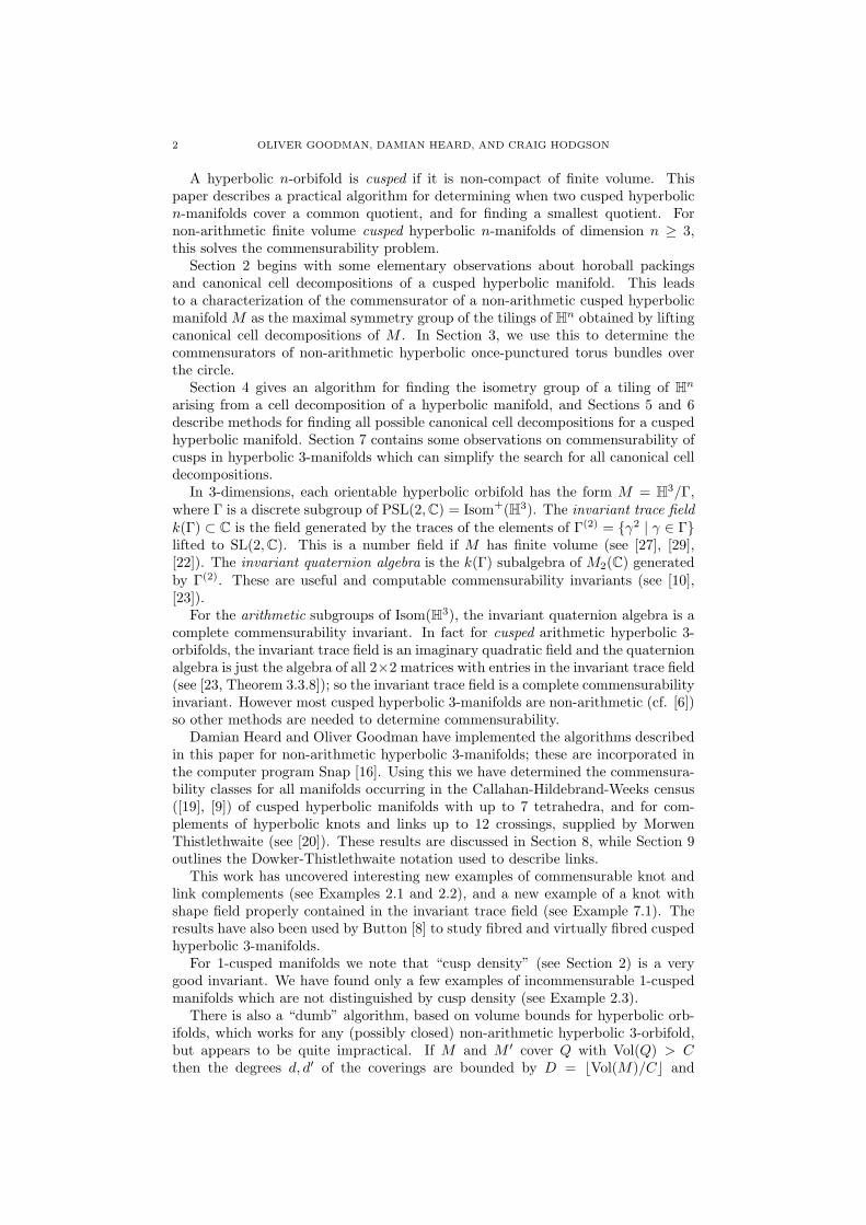
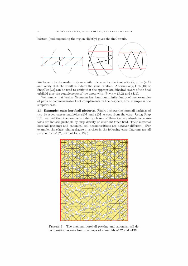
2.3. Example: cusp horoball pictures. Figure 1 shows the horoball packings oftwo 1-cusped census manifolds m137 and m138 as seen from the cusp. Using Snap[16], we find that the commensurability classes of these two equal-volume mani-folds are indistinguishable by cusp density or invariant trace field. Their maximalhoroball packings and canonical cell decompositions are however different. (Forexample, the edges joining degree 4 vertices in the following cusp diagrams are allparallel for m137, but not for m138.)
Figure 1. The maximal horoball packing and canonical cell de-composition as seen from the cusps of manifolds m137 and m138.
COMMENSURATORS OF CUSPED HYPERBOLIC MANIFOLDS 9
3. Example: punctured torus bundles
The bundles over S1 with a once-punctured torus as fibre provide an interestingfamily of 1-cusped hyperbolic 3-manifolds with known canonical triangulations.By analysing how symmetries of the lifted triangulations of the universal coverappear when viewed from the cusp we obtain (in all the non-arithmetic cases)strong constraints on what symmetries may be possible. We then show that theyall come from symmetries of the manifold. This leads to the following:
Theorem 3.1. Let M = H3/G be an orientable non-arithmetic hyperbolic 3-manifold which is a once-punctured torus bundle over S1. Then M has no “hiddensymmetries”, i.e. the commensurator of G is the normalizer of G in Isom(H3).
Let F denote a once-punctured torus, and let ϕ : F → F be an orientationpreserving homeomorphism. Let
M = Mϕ = F ×ϕ S1 =F × [0, 1]
(x, 0) ∼ (ϕ(x), 1)
be the mapping torus of ϕ. Identifying F with (R2 − Z2)/Z2, we have that ϕ isisotopic to an element of SL(2,Z); since M depends only on the isotopy class ofϕ we assume ϕ ∈ SL(2,Z). Then M is hyperbolic whenever ϕ is hyperbolic, i.e.when ϕ has distinct real eigenvalues; Mϕ and Mϕ′ are homeomorphic if and onlyif ϕ and ϕ′ are conjugate.
Define matrices
L =(
1 01 1
), R =
(1 10 1
).
For each word w in the symbols L,R define ϕw ∈ SL(2,Z) as the correspondingmatrix product.
Lemma 3.2. Each ϕ ∈ SL(2,Z) is conjugate to ±ϕw for some word w in thesymbols L,R. The sign is unique and w is determined up to cyclic permutations ofits letters.
Let M = Mϕ where ϕ = ±ϕw is hyperbolic. The so-called monodromy trian-gulation T of M has one tetrahedron for each letter in w and gluings determinedby w and the sign. It is nicely described in [12] and [14]. It follows from work ofLackenby [21] that T is the canonical ideal cell decomposition of M . Other proofs ofthis result have recently been given by Gueritaud ([14], [15]) and Akiyoshi, Sakuma,Wada and Yamashita (see [5]).
The intersection of T with a (small) torus cross section of the cusp of M , lifted toits universal cover R2, gives the (lifted) cusp triangulation T0 of M . Note that edgesand vertices of T0 correspond to edges of T seen transversely or end-on respectively.SnapPea [34] provides pictures of these cusp triangulations: see Figure 3 for anexample.
We need two things: the first is a combinatorial description of T0 in terms of w;the second is an understanding of which edges and vertices of T0 correspond to thesame edges of T in M . Both are outlined briefly here: for detailed explanations werefer the reader to the Appendix of [12] and Sections 3 and 4 of [14].
3.1. The monodromy triangulation T . The triangulation T is built up in layersby gluing tetrahedra according to the letters of w. We begin with an almost flatideal tetrahedron projecting onto a punctured torus; the tetrahedron has edgesa, b, c, c− identified as shown below.

10 OLIVER GOODMAN, DAMIAN HEARD, AND CRAIG HODGSON
a
b b
a
cc-
For each successive letter L or R in the word w, we attach a tetrahedron to thetop of the previous tetrahedron, as shown below in the cover (R2 − Z2)× R.
L
R
a′b′
a
b c
c′
a′
b′
c
c′
After using all the letters of w, the final triangulation of the fibre F differs fromthe initial triangulation by the monodromy ϕ, and we can glue the top and bottomtogether to obtain an ideal triangulation T of M .
3.2. Combinatorial description of T0. Now consider the induced triangulationof a cusp linking torus (i.e. cusp cross section) in M . Each tetrahedron contributesa chain of 4 triangles going once around the cusp as shown in Figure 2.
a
b c
a
b c
a
b c
a
b c
a a
b
b
a
a
b
b
c
a
b
c
b
c
a
b
c
a
b
b
b
a
a
c-
c-
c-
c-
c- c-
c-
c-
c
c-
Figure 2. The chain of triangles around a cusp coming from one tetrahedron.
In the triangulation T0 of R2 this lifts to an infinite chain of triangles forming a(vertical) saw-tooth pattern.
COMMENSURATORS OF CUSPED HYPERBOLIC MANIFOLDS 11
Each chain is glued to the next in one of two ways depending on whether theletter is an L or an R.
RL
Before gluing we adjust slightly the “front” triangles of the first chain and the“back” triangles of the second, so as to create two horizontal edges. After stackingthese chains of triangles together we have a decomposition of T0 into horizontalstrips which can be described combinatorially as follows.
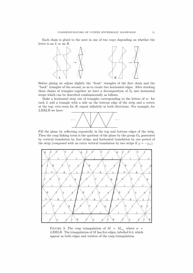
Make a horizontal strip out of triangles corresponding to the letters of w: foreach L add a triangle with a side on the bottom edge of the strip and a vertexat the top; vice-versa for R; repeat infinitely in both directions. For example, forLRRLR we have:
. . . . . .
Fill the plane by reflecting repeatedly in the top and bottom edges of the strip.Then the cusp linking torus is the quotient of the plane by the group G0 generatedby vertical translation by four strips, and horizontal translation by one period ofthe strip (composed with an extra vertical translation by two strips if ϕ = −ϕw).
3 3
0
2
3
0
2
3
0
22
1
0
2
1
0
2
1
03 0 2 3 0 2 3 0 2 3
1 0 2 1 0 2 1 0 2
0
2
1
0
2
1
0
2
1
0
2
0
2
0
2
2
3
0
2
3
0
2
3
0
3
0
3
0
3
0
1
0
1
0
1
0
2
1
0
2
1
0
2
1
0
3 0 2 3 0 2 3 0 2
0 2 3 0 2 3 0 2 3
3
0
3
0
3
0
3
0
2
3
0
2
3
0
2
0
2
1
0
2
1
0
2
12
3
0
2
3
0
2
3
0
1 0 2 1 0 2 1 0 2
4 432 432 32
3
2
4
3
2
4
3
2
4
3
4
3
2
4
3
2
4
3
2
4
4
3
4
3
4
3
3
2
3
2
3
2
3
2
4
3
2
4
3
2
4432 432 432
3
2
4
3
2
4
3
2
4
3
134 134 134
3
4
1
3
4
1
3
4
1
3
4
1
3
4
1
3
4
1
3
1
3
1
3
1
3
3
4
3
4
3
4
4
1
3
4
1
3
4
1
3
13 134 134 4
1
3
4
1
3
4
1
3
4
1
30
3
1
0
3
1
0
3
1
3 1 0 3 1 0 3 1 0 3
1
0
3
1
0
3
1
0
3
0 0
3
0
3
0
3
3 1 0 3 1 0 3 1 0
1 0 3 1 0 3 1 0 3
0
3
0
3
0
3
0
3
1
0
3
1
0
3
11
0
3
1
0
3
1
0
3 3
Figure 3. The cusp triangulation of M = Mϕwwhere w =
LRRLR. The triangulation ofM has five edges, labelled 0-4, whichappear as both edges and vertices of the cusp triangulation.
12 OLIVER GOODMAN, DAMIAN HEARD, AND CRAIG HODGSON
3.3. Edge/vertex correspondence in T0. To understand which edges of T0 areidentified in T , we define a “direction” on each horizontal strip: right to left on thefirst strip, left to right on the strips below and above it, and so on, so that adjacentstrips have opposite directions. Then we have:
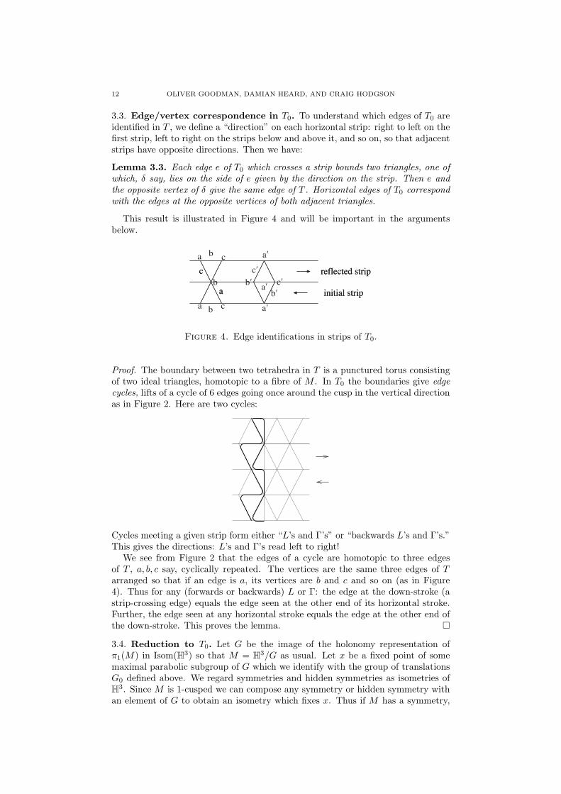
Lemma 3.3. Each edge e of T0 which crosses a strip bounds two triangles, one ofwhich, δ say, lies on the side of e given by the direction on the strip. Then e andthe opposite vertex of δ give the same edge of T . Horizontal edges of T0 correspondwith the edges at the opposite vertices of both adjacent triangles.
This result is illustrated in Figure 4 and will be important in the argumentsbelow.
initial strip
reflected stripc
a
b
b
binitial strip
reflected stripc
c
a
a
a
cb′
c′
a′
a′
a′
b′ c′
Figure 4. Edge identifications in strips of T0.
Proof. The boundary between two tetrahedra in T is a punctured torus consistingof two ideal triangles, homotopic to a fibre of M . In T0 the boundaries give edgecycles, lifts of a cycle of 6 edges going once around the cusp in the vertical directionas in Figure 2. Here are two cycles:
Cycles meeting a given strip form either “L’s and Γ’s” or “backwards L’s and Γ’s.”This gives the directions: L’s and Γ’s read left to right!
We see from Figure 2 that the edges of a cycle are homotopic to three edgesof T , a, b, c say, cyclically repeated. The vertices are the same three edges of Tarranged so that if an edge is a, its vertices are b and c and so on (as in Figure4). Thus for any (forwards or backwards) L or Γ: the edge at the down-stroke (astrip-crossing edge) equals the edge seen at the other end of its horizontal stroke.Further, the edge seen at any horizontal stroke equals the edge at the other end ofthe down-stroke. This proves the lemma. �
3.4. Reduction to T0. Let G be the image of the holonomy representation ofπ1(M) in Isom(H3) so that M = H3/G as usual. Let x be a fixed point of somemaximal parabolic subgroup of G which we identify with the group of translationsG0 defined above. We regard symmetries and hidden symmetries as isometries ofH3. Since M is 1-cusped we can compose any symmetry or hidden symmetry withan element of G to obtain an isometry which fixes x. Thus if M has a symmetry,
COMMENSURATORS OF CUSPED HYPERBOLIC MANIFOLDS 13
it is represented by a symmetry of T0; if it has a non-trivial hidden symmetry, it isrepresented by a symmetry of T0 which does not come from a symmetry of M .
Since our combinatorial picture of T0 is not metrically exact, we only know thatsymmetries and hidden symmetries act as simplicial homeomorphisms (S.H.) of T0.
Lemma 3.4. Simplicial homeomorphisms of T0 preserve horizontal strips wheneverw 6= (LR)m or (LLRR)m as a cyclic word, for any m > 0.
Since vertex orders in T0 are all even we can define a straight line to be a pathin the 1-skeleton which enters and leaves each vertex along opposite edges. A stripconsists of a part of T0 between two (infinite, disjoint) straight lines such that everyinterior edge crosses from one side of the strip to the other.
Proof. If an edge of T0 lies on the edge of a strip, not necessarily horizontal, theopposite vertex of the triangle which crosses that strip must have order at least 6:the straight line going through this vertex has at least the two edges of the triangleon one side.
If there exists an S.H. which is not horizontal strip preserving, every vertex of T0
will lie on a non-horizontal edge which is an edge of some strip (namely the imageof a previously horizontal strip edge).
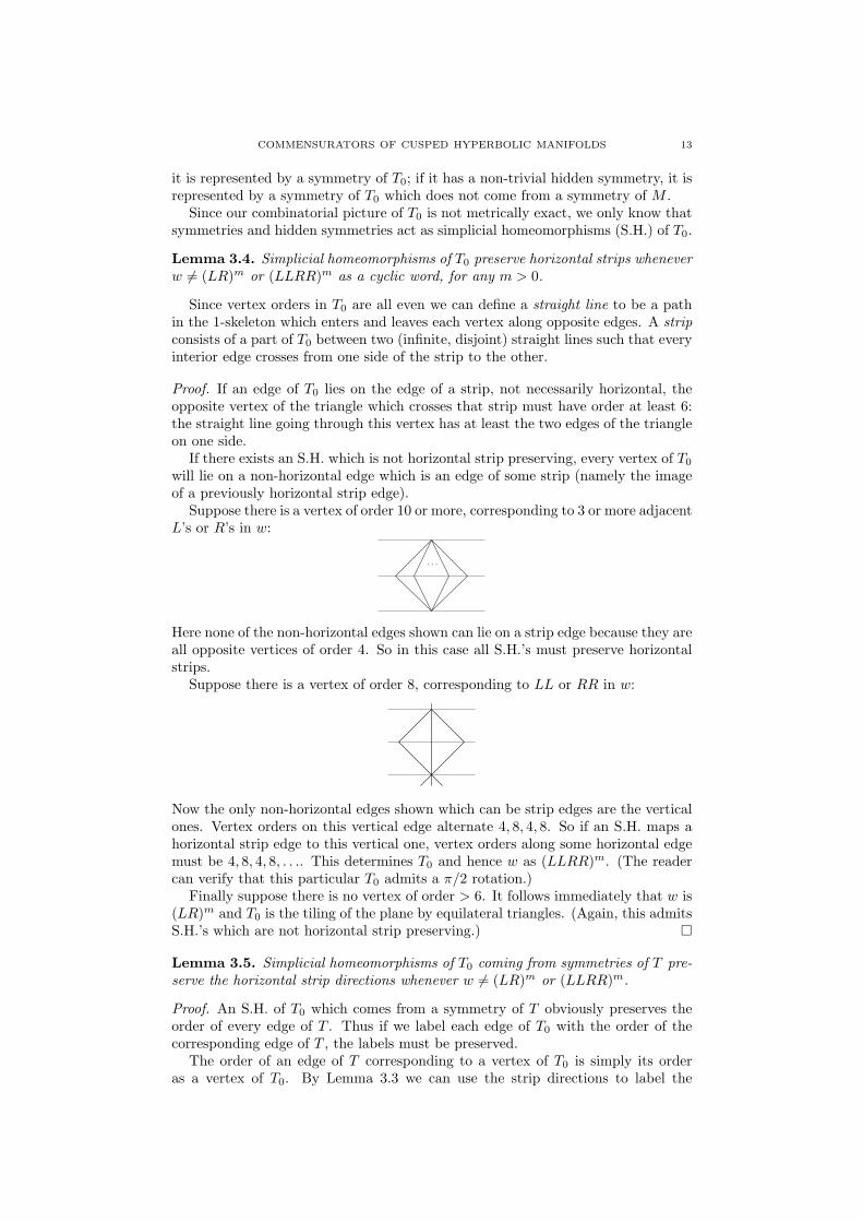
Suppose there is a vertex of order 10 or more, corresponding to 3 or more adjacentL’s or R’s in w:
. . .
Here none of the non-horizontal edges shown can lie on a strip edge because they areall opposite vertices of order 4. So in this case all S.H.’s must preserve horizontalstrips.
Suppose there is a vertex of order 8, corresponding to LL or RR in w:
Now the only non-horizontal edges shown which can be strip edges are the verticalones. Vertex orders on this vertical edge alternate 4, 8, 4, 8. So if an S.H. maps ahorizontal strip edge to this vertical one, vertex orders along some horizontal edgemust be 4, 8, 4, 8, . . .. This determines T0 and hence w as (LLRR)m. (The readercan verify that this particular T0 admits a π/2 rotation.)
Finally suppose there is no vertex of order > 6. It follows immediately that w is(LR)m and T0 is the tiling of the plane by equilateral triangles. (Again, this admitsS.H.’s which are not horizontal strip preserving.) �
Lemma 3.5. Simplicial homeomorphisms of T0 coming from symmetries of T pre-serve the horizontal strip directions whenever w 6= (LR)m or (LLRR)m.
Proof. An S.H. of T0 which comes from a symmetry of T obviously preserves theorder of every edge of T . Thus if we label each edge of T0 with the order of thecorresponding edge of T , the labels must be preserved.
The order of an edge of T corresponding to a vertex of T0 is simply its orderas a vertex of T0. By Lemma 3.3 we can use the strip directions to label the

14 OLIVER GOODMAN, DAMIAN HEARD, AND CRAIG HODGSON
corresponding edges of T0. Given a vertex of order 10 or more we have:
4 . . .4 ?
6+
? 46+ 4
The direction on a horizontal strip cannot be reversed because this would swap anedge of order 4 with one of order 6 or more.
Suppose now the maximum vertex order is 8. For each order 8 vertex we have:
4
4
If there is an S.H. which reverses strip direction then the other two sides of thisdiamond figure, wherever it appears, must also be labelled with 4’s.
44
The 4 on the upper right edge implies that the right hand vertex of the diamondhas order ≥ 8, hence 8. This gives another diamond figure adjacent to the first one.The argument can be repeated giving the pattern associated with w = (LLRR)m.
If there are no vertices of order > 6, w = (LR)m. �
Proof of Theorem 3.1. It is shown in [7] that the only arithmetic orientable hy-perbolic punctured torus bundles are those for which w = LR,LLR (or LRR)or LLRR, or powers of these, having invariant trace fields Q(
√−3),Q(
√−7) and
Q(√−1) respectively. Thus, in the non-arithmetic cases, Lemmas 3.4 and 3.5 show
that all symmetries of T0 which come from hidden symmetries of M are representedby simplicial homeomorphism which preserve the strips and strip-directions.
Note that there are two “sister” manifolds for each w depending on whetherthe monodromy is ϕw or −ϕw; the triangulations of H3 however are the same,depending only on w.
It is now easy to see that the possible symmetries of T0, modulo the translationsin G0, are restricted to the types listed below. We show that each, if it occurs atall, comes from an actual symmetry of M .
(1) Shifting up or down by two strips. This is realized by the symmetry(−1 0
0 −1
)× 1 from F ×±ϕw
S1 to itself. (Note that(−1 0
0 −1
)is central in SL(2,Z).)
ϕw
(−1 0
0 −1
)× 1
ϕw

COMMENSURATORS OF CUSPED HYPERBOLIC MANIFOLDS 15
(2) If w is a power, w = um, then T0 admits a horizontal translation by `(u)triangles, where `(u) is the length of the word u. In this case
ϕu
ϕu
ϕu
M =
and 1 × r2π/m gives a symmetry of order m (where rθ denotes rotation ofthe unit circle S1 by θ). For the −ϕw case we replace one of the ϕu’s by−ϕu. After rotating we also have to apply −1× 1 to F × [0, 1/m].
(3) If w is palindromic, i.e. w and its reverse w′ are the same as cyclic words,then T0 admits a rotation by π about a point on one of the strip edges. This
is realized by(
1 00 −1
)× refl(S1), where refl(S1) denotes a reflection of
S1.ϕw
1× refl(S1)
ϕ−1w
(1 00 −1
)× 1
ϕw′
Note that conjugation by(
1 00 −1
)takes L to L−1 and R to R−1.
(4) If `(w) is even and rotating w by a half turn swaps L’s and R’s, T0 has aglide reflection mapping a strip to itself, exchanging the top and bottom
of the strip. This is realized by(
0 11 0
)× 1 since conjugation by this
matrix swaps L and R. More explicitly, let w = uv where v is u with L’sand R’s interchanged. The symmetry is
ϕu
ϕv
(0 11 0
)× 1
ϕv
ϕu
followed by rπ on the S1 factor. This symmetry is orientation reversing.(5) If `(w) is even and reversing w swaps L’s and R’s (we might say that w
is anti-palindromic) then T0 admits a glide reflection with vertical axis,
shifting everything up by one strip. This is realized by(
0 1−1 0
)×
refl(S1) since conjugation by(
0 1−1 0
)takes L to R−1 and R to L−1.
This symmetry is orientation reversing. We leave the picture as an exercisefor the reader.
�
Clearly if M admits any two of the symmetries 3–5 it admits the third which isa product of the other two. Thus if w is not a power, M may have one of 5 possiblesymmetry groups.

16 OLIVER GOODMAN, DAMIAN HEARD, AND CRAIG HODGSON
4. Algorithm for finding isometries of tilings
To apply our commensurability criterion, Theorem 2.4, we need a way to deter-mine when tilings of Hn, arising from ideal cell decompositions, are isometric. Wepursue this question in a slightly more general setting.
Let M and M ′ be geometric n-manifolds with universal cover Xn = En orHn, each with a given finite decomposition into convex polyhedra. We wish todetermine whether the tilings T and T ′ which cover these two cell decompositionsare isometric. (The elements of T (resp. T ′) are convex polyhedra in Xn whichproject to polyhedra in the decomposition of M (resp. M ′).)
Necessary and sufficient conditions for the tilings to be isometric are as follows.(1) There is an isometry i of Xn which maps an element of T isometrically
onto an element of T ′.(2) Whenever i maps P ∈ T isometrically onto P ′ ∈ T ′, and F is a (codimen-
sion 1) face of P , i maps the neighbour of P at F isometrically onto theneighbour of P ′ at i(F ).
Sufficiency follows from the fact that we can proceed from any tile in T to any otherby a finite sequence of steps between neighbouring tiles.
Let S and S′ denote the polyhedra decomposing M and M ′ respectively.Let Θ denote the set of all triples (j, p, p′), where p ∈ S, p′ ∈ S′, and j is an
isometry carrying p onto p′. We can find Θ in a finite number of steps. Condition 1above is equivalent to Θ being non-empty.
We say that (j, p, p′) ∈ Θ is induced by an isometry i of Xn if there exist P ∈ Tprojecting to p and P ′ ∈ T ′ projecting to p′ such that i carries P isometricallyonto P ′ and the restriction induces j. Let f be a face of p and let q and q′ be theneighbours of p and p′ at f and j(f) respectively. The restriction of j to f inducesan isometry between certain faces of q and q′. If this extends to (jq, q, q′) we saythat (j, p, p′) extends across f to (jq, q, q′). If (j, p, p′) is induced by i then (jq, q, q′)will be also.
Condition 2 is equivalent to the following: whenever (j, p, p′) is induced by i,and f is a face of p, then (j, p, p′) extends across f .
Theorem 4.1. With the above notation, the tilings T and T ′ are isometric if andonly if there exists a non-empty subset I of Θ such that every element of I extendsacross each of its faces to yield another element of I.
Proof. If T and T ′ are isometric with isometry i, simply let I be the set of elementsof Θ induced by i.
Conversely, suppose we have I ⊆ Θ having the stated properties. Choose anyelement (j, p, p′) ∈ I and any isometry i of Xn which induces it. Clearly condition 1above is satisfied. For condition 2 note that if i maps P onto P ′ and this induces(j, p, p′) ∈ I then, because this extends across all of its faces, i maps neighbours ofP isometrically onto neighbours of P ′ and these too induce elements of I. Thereforecondition 2 is satisfied with all the induced triples belonging to I. �
An algorithm for finding such a subset I ⊆ Θ or establishing that none existsis straightforward. If Θ is empty, stop; there is no such subset. Otherwise chooseany element of Θ and put it in I. For each element of I check if we can extendacross all faces. If we can’t, remove all elements of I from Θ and start again. Ifwe can, and every element we reach is already in I, stop and output I. If we canextend across faces of all elements of I, and we obtain new elements not yet in I,add those new elements to I and check again.
Each set I found by the algorithm represents an equivalence class of isometriescarrying T onto T ′: choose an isometry i inducing any element of I; then isometries
COMMENSURATORS OF CUSPED HYPERBOLIC MANIFOLDS 17
i, i′ are equivalent if i′ = g′ig where g is a covering transformation of M and g′ isa covering transformation of M ′.
To find the symmetry group of a tiling T we apply the algorithm with T = T ′,M = M ′ etc. Let Γ denote the group of covering transformations of M . Repeatingthe algorithm until Θ is exhausted we obtain finitely many equivalence classes ofsymmetries. These represent the double cosets of Γ in Symm(T ). Together with Γthey generate Symm(T ).
Remark 4.2. Each set I found by this algorithm also represents a common coveringN of M and M ′ constructed as follows: For each element r = (j, p, p′) ∈ I let prdenote a copy of p. Let N be the disjoint union of the polyhedra pr as r varies overI, with the following face identifications. Each face f of p appears as a face fr ofpr. Whenever r extends across f to s = (jq, q, q′), identify face fr of pr with facefs of qs.
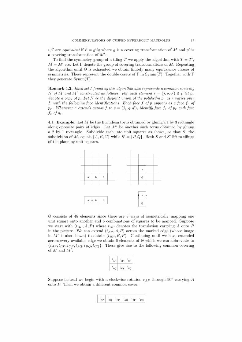
4.1. Example. Let M be the Euclidean torus obtained by gluing a 1 by 3 rectanglealong opposite pairs of edges. Let M ′ be another such torus obtained by gluinga 2 by 1 rectangle. Subdivide each into unit squares as shown, so that S, thesubdivision of M , equals {A,B,C} while S′ = {P,Q}. Both S and S′ lift to tilingsof the plane by unit squares.
A B C
A B C
Q
P
Q
P
Θ consists of 48 elements since there are 8 ways of isometrically mapping oneunit square onto another and 6 combinations of squares to be mapped. Supposewe start with (tAP , A, P ) where tAP denotes the translation carrying A onto Pin the picture. We can extend (tAP , A, P ) across the marked edge (whose imagein M ′ is also shown) to obtain (tBP , B, P ). Continuing until we have extendedacross every available edge we obtain 6 elements of Θ which we can abbreviate to{tAP , tBP , tCP , tAQ, tBQ, tCQ}. These give rise to the following common coveringof M and M ′.
APt t t
t t t
BP CP
AQ BQ CQ
Suppose instead we begin with a clockwise rotation rAP through 90◦ carrying Aonto P . Then we obtain a different common cover.
BQ BPrAP
r rCP
rAQ
r rCQ
18 OLIVER GOODMAN, DAMIAN HEARD, AND CRAIG HODGSON
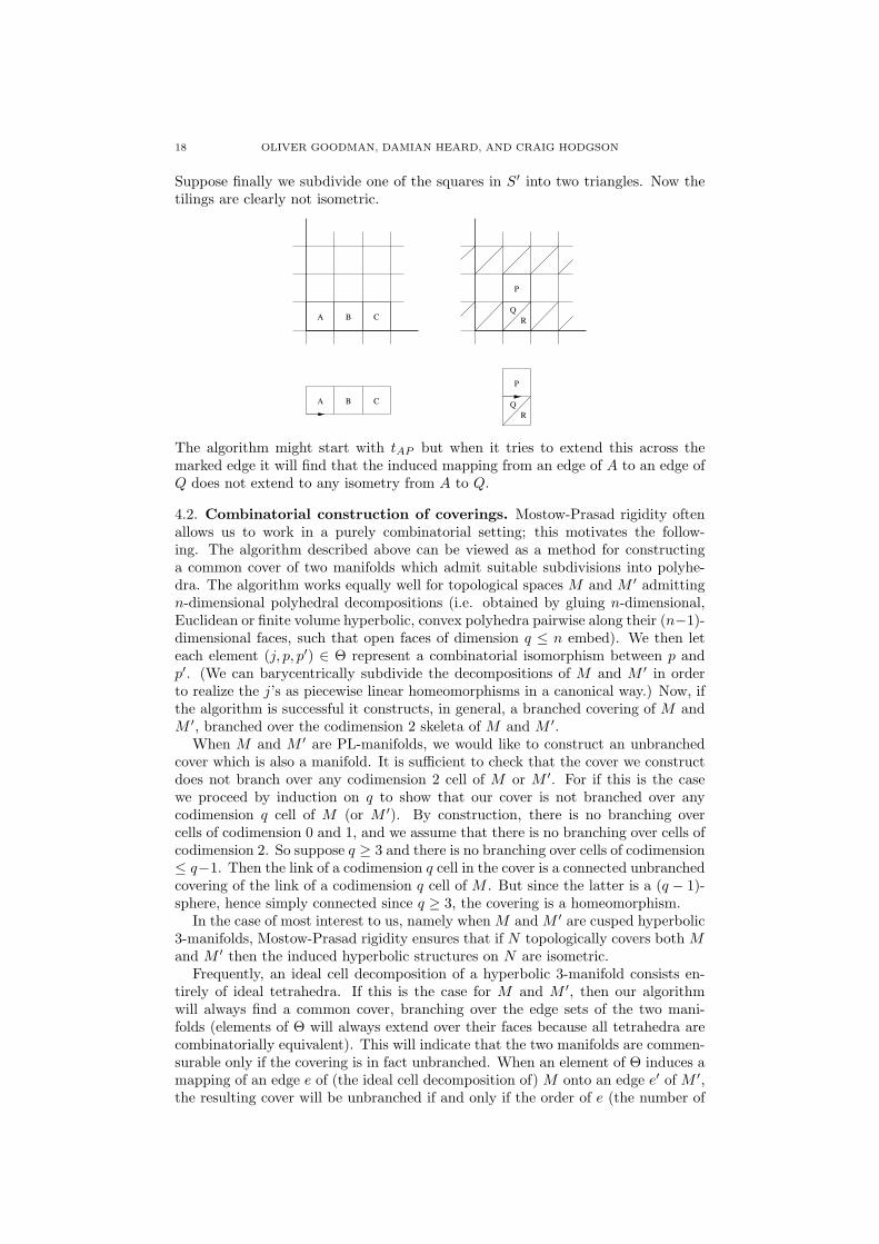
Suppose finally we subdivide one of the squares in S′ into two triangles. Now thetilings are clearly not isometric.
A B C
A B C
RQ
P
P
RQ
The algorithm might start with tAP but when it tries to extend this across themarked edge it will find that the induced mapping from an edge of A to an edge ofQ does not extend to any isometry from A to Q.
4.2. Combinatorial construction of coverings. Mostow-Prasad rigidity oftenallows us to work in a purely combinatorial setting; this motivates the follow-ing. The algorithm described above can be viewed as a method for constructinga common cover of two manifolds which admit suitable subdivisions into polyhe-dra. The algorithm works equally well for topological spaces M and M ′ admittingn-dimensional polyhedral decompositions (i.e. obtained by gluing n-dimensional,Euclidean or finite volume hyperbolic, convex polyhedra pairwise along their (n−1)-dimensional faces, such that open faces of dimension q ≤ n embed). We then leteach element (j, p, p′) ∈ Θ represent a combinatorial isomorphism between p andp′. (We can barycentrically subdivide the decompositions of M and M ′ in orderto realize the j’s as piecewise linear homeomorphisms in a canonical way.) Now, ifthe algorithm is successful it constructs, in general, a branched covering of M andM ′, branched over the codimension 2 skeleta of M and M ′.
When M and M ′ are PL-manifolds, we would like to construct an unbranchedcover which is also a manifold. It is sufficient to check that the cover we constructdoes not branch over any codimension 2 cell of M or M ′. For if this is the casewe proceed by induction on q to show that our cover is not branched over anycodimension q cell of M (or M ′). By construction, there is no branching overcells of codimension 0 and 1, and we assume that there is no branching over cells ofcodimension 2. So suppose q ≥ 3 and there is no branching over cells of codimension≤ q−1. Then the link of a codimension q cell in the cover is a connected unbranchedcovering of the link of a codimension q cell of M . But since the latter is a (q − 1)-sphere, hence simply connected since q ≥ 3, the covering is a homeomorphism.
In the case of most interest to us, namely when M and M ′ are cusped hyperbolic3-manifolds, Mostow-Prasad rigidity ensures that if N topologically covers both Mand M ′ then the induced hyperbolic structures on N are isometric.
Frequently, an ideal cell decomposition of a hyperbolic 3-manifold consists en-tirely of ideal tetrahedra. If this is the case for M and M ′, then our algorithmwill always find a common cover, branching over the edge sets of the two mani-folds (elements of Θ will always extend over their faces because all tetrahedra arecombinatorially equivalent). This will indicate that the two manifolds are commen-surable only if the covering is in fact unbranched. When an element of Θ induces amapping of an edge e of (the ideal cell decomposition of) M onto an edge e′ of M ′,the resulting cover will be unbranched if and only if the order of e (the number of
COMMENSURATORS OF CUSPED HYPERBOLIC MANIFOLDS 19
tetrahedra to which glue around it) is equal to the order of e′. For example, thishas the following corollary.
Theorem 4.3. If a finite volume hyperbolic 3-manifold M admits a decompositioninto ideal tetrahedra such that the order of every edge is 6, then M is commensurablewith the complement of the figure-8 knot.
5. Enumerating canonical cell decompositions I
For 1-cusped hyperbolic manifolds with discrete commensurator we now haveall the ingredients of an effective method for testing commensurability. For multi-cusped manifolds we need a way to search through the (finite) set of all canonicalideal cell decompositions. In this section and the next we describe two alternativeapproaches to this problem, while in Section 7 we show how the search can berestricted for greater efficiency.
The first approach is very simple minded: if we can bound the degree with whichM covers its commensurator quotient, we can enumerate all cusp cross sectionswhich could possibly cover equal area cross sections in the quotient. Such degreebounds can be obtained from estimates on the the minimum volume of cuspednon-arithmetic hyperbolic 3-manifolds ([26], [1], [28]).
The second approach is geometric and may be of more theoretical interest sinceit truly finds all the canonical cell decompositions. In fact it associates with a givenc-cusped M , a convex polytope in Rc whose k-dimensional faces, for 0 ≤ k < c, arein 1-1 correspondence with canonical cell decompositions of M .
Let M be a hyperbolic orbifold with (horoball) cusp neighbourhoods C1, . . . , Cmand let N be a degree d quotient of M with corresponding cusp neighbourhoodsc1, . . . , cn. Let π : M → N be the covering projection and let cj(i) = π(Ci). If wechoose horospherical cross sections in N with “area” (i.e. codimension 1 volume)equal to 1, the area of ∂Ci is equal to the degree with which Ci covers cj(i). Thesum of the areas of the Ci covering cj will be d for each cj .
Thus, in order to find a possible degree d quotient of M via the canonical celldecomposition, we can enumerate the possible integer area vectors as follows. Foreach n, 1 ≤ n ≤ m, and each partition of {1, . . . ,m} into n non-empty subsetsI1, . . . , In, enumerate all area vectors (a1, . . . , am) such that each ai is a positiveinteger and
∑i∈Ij
ai = d for j = 1, . . . , n.Example: if m = 3 we have partitions {{1, 2, 3}}, {{1, 2}, {3}}, {{1, 3}, {2}},
{{1}, {2, 3}} and {{1}, {2}, {3}}. The first partition admits 12 (d − 1)(d − 2) area
vectors, the next three admit d− 1 each, and the last, just one.We can enumerate area vectors corresponding to possible quotients of degree d
as follows. Any quotient of M of degree d has n ≤ m cusps and has a correspondingarea vector (a1, . . . , am) with sum
∑mi=1 ai = nd. So if we fix an integer D ≥ m
and enumerate all positive integer area vectors summing to at most D, we willfind all quotients of degree d with n ≤ m cusps such that nd ≤ D. In particularthis will include all quotients with at most m − 1 cusps provided d ≤ D/(m − 1).Since the canonical cell decomposition is determined by the ratio of the areas, anym cusped quotient is found using the area vector (1, . . . , 1) with
∑i ai = m ≤ D.
So we will find all canonical cell decompositions arising from quotients of degreed ≤ D/(m− 1).
6. Enumerating canonical cell decompositions II
Let M be a hyperbolic n-manifold with c > 0 cusps. Then the set of possiblechoices of (not necessarily disjoint) horospherical cross sections dual to the cusps ofM is parametrized by the vector of their areas (i.e. (n − 1)-dimensional volumes)
20 OLIVER GOODMAN, DAMIAN HEARD, AND CRAIG HODGSON
in Rc>0 = {(v1, . . . , vc) ∈ Rc | v1 > 0, . . . , vc > 0}. In fact it turns out to be moreconvenient to parametrize by the (n− 1)th root of area, a quantity we will refer toas size. Multiplying a size vector v ∈ Rc>0 by a constant λ > 0 has the effect ofshifting the corresponding horospherical cross sections a distance log(λ) down (i.e.away from) the cusps.
For each v ∈ Rc>0 we obtain a Ford spine. It is clear from the definition that ifwe choose a set of disjoint horospherical cross sections and then shift them all upor down by the same amount we get the same Ford spine. Thus the set of possibleFord spines is parametrized by the set of rays in Rc>0, or equivalently, by points inthe open (c− 1)-dimensional simplex S = {(v1, . . . , vc) ∈ Rc>0 | v1 + · · ·+ vc = 1}.For a 1-cusped manifold the Ford spine is unique.
Dual to each Ford spine is a canonical cell decomposition D(v). As we varyv ∈ S the decomposition changes only when the combinatorics of the spine changes.To better understand this dependence we now review an alternative approach todefining D(v), namely the original one of Epstein-Penner in [11].
We work in Minkowski space En,1 with the inner product ∗ defined by
x ∗ y = x1y1 + . . .+ xnyn − xn+1yn+1
for x = (x1, . . . , xn+1), y = (y1, . . . , yn+1) in Rn+1. Then hyperbolic space Hn isthe upper sheet of the hyperboloid x ∗ x = −1, and the horospheres in Hn arerepresented by the intersections of hyperplanes, having light-like normal vectors,with Hn. Each such hyperplane H has a unique Minkowski normal n such thatx ∈ H if and only if x ∗ n = −1.
Let Γ denote the group of covering transformations of Hn over M . Each sizevector v gives rise to a Γ-invariant set of horospheres in Hn. The resulting setof normals in Minkowski space is invariant under the action of the group Γ. Theconvex hull of this set of points, which we shall refer to as the Epstein-Pennerconvex hull, intersects every ray based at the origin passing through a point in theupper sheet of the hyperboloid. The boundary of this convex set is a union ofclosed convex n-dimensional polytopes having coplanar light-like vertices. Epsteinand Penner [11] show that these project to a locally finite, Γ-invariant set of idealpolyhedra in Hn, which in turn project to a finite set D(v) of ideal hyperbolicpolyhedra in M .
Starting with a given ideal hyperbolic cell decomposition D of M and a sizevector v, we proceed next to describe necessary and sufficient conditions for D tobe the canonical cell decomposition D(v), as in [33] and [30].
Let C be a cell of D. Then v determines a horospherical cross section to eachideal vertex of C. We lift C and this choice of horospheres to Hn. In Minkowskispace, this gives a convex (Euclidean) n-dimensional polytope whose vertices arethe hyperplane normals for these horospheres. Whenever C is not a simplex, it isnecessary to add the condition that these vertices are coplanar. If this is satisfiedfor all the non-simplicial cells of D, we can lift each cell to an n-dimensional poly-tope in Minkowski space with vertices corresponding to the choice of horospheresdetermined by the size vector v. If C and C ′ are neighbouring cells in D it is nec-essary that the angle between neighbouring lifts into Minkowski space be convexupwards. Together these conditions are also sufficient to imply D = D(v).
These conditions can be expressed as a set of linear equations and linear inequal-ities on the entries of the size vector v.
Proposition 6.1. Let D be an ideal hyperbolic cell decomposition of a cusped hy-perbolic n-manifold M with c cusps. Then there exist matrices LD and FD with ccolumns such that, for v ∈ Rc>0, D(v) = D if and only if LDv = 0 and FDv > 0.
COMMENSURATORS OF CUSPED HYPERBOLIC MANIFOLDS 21
Note: here v is written as a column vector, and the condition FDv > 0 means thateach entry of the vector FDv is positive.
Proof. Let vi denote the entry of v corresponding to the ith cusp of M . Let nj bethe vertex representative for the jth vertex of C lifted to Minkowski space for thechoice of horospheres given by v = (1, . . . , 1). Then for an arbitrary size vector vthe corresponding representative is nj/vc(j), where c(j) is the cusp of the jth vertexof C.
The coplanarity condition on a non-simplicial cell C gives a set of linear equa-tions satisfied by v, one for each vertex of C in excess of n + 1, as follows. LetNv be a Euclidean normal to the hyperplane containing {n0/vc(0), . . . ,nn/vc(n)}such that (nj/vc(j)) · Nv = 1 for j = 0, . . . , n, where · denotes the Euclideandot product. Writing MC for the inverse of the matrix with rows nj we obtainNv = MC(vc(0), . . . , vc(n))t, which is a linear function of v. For j > n, nj/vc(j)belongs to this hyperplane if and only if nj · Nv − vc(j) = 0, which is linear in v.The full set of constraints for C gives a matrix equation LCv = 0.
The convexity condition at an (n − 1)-cell f of D, being the common face ofn-cells C and C ′, can be expressed as follows. Let Nv, as above, be the definingnormal for the hyperplane containing the lift of C determined by v. Let n′k/vc(k)be a vertex of an adjacent lift of C ′, not in the lift of f . This vertex lies above thehyperplane if and only if (n′k/vc(k)) · Nv > 1, or equivalently n′k · Nv − vc(k) > 0.We refer to the left-hand side of this inequality as the tilt at f of v and express thecondition as Ffv > 0, where Ff is a suitable row-vector. (Note that the sign of ourtilt function is opposite to that of [33] and [31].)
Finally, concatenate the matrices LC into a matrix LD and the rows Ff into amatrix FD. �
Let PD denote the set of v ∈ Rc>0 such that LDv = 0 and FDv > 0. We callthis the parameter cell of D since it contains all cusp size parameters v such thatD(v) = D. Each v ∈ Rc>0 belongs to a parameter cell, namely P(v) = PD(v). Theparameter cell PD is non-empty if and only if D is a canonical cell decomposition.
It is shown in [4] that the number of canonical cell decompositions is finite.Therefore Rc>0 is a union of finitely many parameter cells.
Proposition 6.2. Each v ∈ Rc>0 can be perturbed to obtain a nearby vector v′ suchthat P(v′) has dimension c and P(v) is a face of P(v′) (or equals P(v) if this hasdimension c).
Proof. Let D = D(v). If LD is zero (or empty) then P(v) is an open subset, hencea c-dimensional cell and we just set v′ = v.
Otherwise, perturb v such that it leaves the linear subspace determined by LDv =0. For a small perturbation the Epstein-Penner convex hull changes as follows: nodihedral angle between adjacent n-faces goes to π but some non-simplicial n-facesmay be subdivided if their vertices become non-coplanar. It follows that LD maylose rows and FD may gain rows. LetD′ be the new decomposition. Then LD′ 6= LDbecause LD′v′ = 0 while LDv′ 6= 0. Repeat until LD′ is zero (or empty). ThenP(v′) has dimension c.
Now v belongs to a face of PD′ since it satisfies Ffv > 0 for each face f commonto D and D′, and Ff ′v = 0 for each face f ′ of D′ not in D. The former conditionamounts to FDv > 0. We have to show that the latter is equivalent to LDv = 0.But that is equivalent to the coplanarity of the lifted vertices of each n-cell of D.Such a cell may be subdivided by new faces f ′ in D′. Then the vertices will becoplanar at v if and only if the tilt at each subdividing face is zero, i.e. if and onlyif Ff ′v = 0 for the subdividing faces. �
22 OLIVER GOODMAN, DAMIAN HEARD, AND CRAIG HODGSON
The above proposition implies that each face of a parameter cell is anotherparameter cell; the decomposition corresponding to a parameter cell is a refinementof the decompositions corresponding to its faces.
Remark 6.3. It is tempting to suppose that the canonical cell decomposition ofM corresponding to a c dimensional parameter cell must consist entirely of idealsimplices but this need not be the case. In general we can have cell decompositionswith non-simplicial cells such that LD is a zero matrix. (For example, this occursfor the Borromean rings complement — see Section 6.1 below.)
We now have the following algorithm for finding all canonical cell decompositions.First we find all the c-dimensional parameter cells.
(1) Choose an arbitrary v ∈ Rc>0.(2) Perturb v if necessary, as in the proof of Proposition 6.2, so that P(v) has
dimension c, and add it to our list of cells.(3) If the closure of the cells we have found so far does not contain the whole of
Rc>0, choose a new v not in the closure of any cell found so far and repeatstep 2.
By the finiteness result quoted above, this algorithm eventually terminates. Wecan then enumerate all canonical cell decompositions by enumerating the faces ofall dimensions of the cells P(v).
While the computational geometry involved in implementing the above algorithmis certainly possible, it is not particularly nice. We explain a refinement which givesa little more insight and an algorithm which is easier to implement.
For a decomposition D of M , let ΣD denote the row vector obtained by addingtogether the rows of FD. We define the tilt polytope of M to be the set of v ∈ Rc>0
such that ΣD · v < 1 for all canonical cell decompositions D of M .
Proposition 6.4. The tilt polytope T of M is bounded. The parameter cells PDof M are the cones over the origin of those faces of T which are not contained in∂Rc>0.
Proof. We show that the closure of a c-dimensional parameter cell PD has boundedintersection with T . Let v be a unit vector in PD. Then since v is not containedin every face of PD, ΣD · v > 0. The length of any multiple of v contained in Tis bounded by 1/(ΣD · v). Since this is continuous in v, and the set of such v iscompact, PD ∩ T is bounded. Since T is a union of finitely many such sets it isbounded.
Let us write HD for the half-space {x ∈ Rc | ΣD · x < 1}. Then T is theintersection of all the HD’s with Rc>0. We will show that: if v belongs to a c-dimensional parameter cell PD, and PD′ is any other parameter cell, then the raygenerated by v leaves HD before it leaves HD′ .
It will then follow that a ray in PD penetrates the (non-empty) face of T gener-ated by HD. Since a ray not in PD belongs to the closure of some other parametercell, it does not leave HD first and therefore does not pass through the same faceof T . Since cones on the lower dimensional faces of a (c − 1)-dimensional faceof T are the faces of a c-dimensional parameter cell, the result then follows fromProposition 6.2.
It remains to show that HD cuts off any ray in PD closer to the origin than HD′ ,for all parameter cells PD′ 6= PD. Equivalently, for v ∈ PD, ΣD · v > ΣD′ · v.
Firstly, let PD and PD′ be any two parameter cells such that PD′ is a face ofPD, and let v belong to PD. The rows of FD′ are a proper subset of the rows ofFD, and since Ff · v > 0 for each row, ΣD · v > ΣD′ · v. If instead PD is a face
COMMENSURATORS OF CUSPED HYPERBOLIC MANIFOLDS 23
of PD′ , then the rows of FD′ omitted from FD are precisely those for which Ff · vvanishes. Therefore in that case ΣD · v = ΣD′ · v.
Next, let PD be a c-dimensional parameter cell, and let PD′ be arbitrary, withD′ 6= D. Choose v ∈ PD and v′ ∈ PD′ . Let PD1 , . . . ,PDm be the parameter cellsthrough which the straight line vt := (1 − t)v + tv′ passes for 0 ≤ t ≤ 1 (so thatD1 = D and Dm = D′). For vt in PDi
, ΣDi· vt ≥ ΣDi+1 · vt while for vt ∈ PDi+1 ,
ΣDi· vt ≤ ΣDi+1 · vt. Since the difference between these terms is (affine) linear in t,
the former inequality must hold for all lesser values of t, in particular, when vt = v.Note also that the first such inequality is strict, namely, ΣD1 ·v > ΣD2 ·v. It followsthat ΣD · v > ΣD′ · v for arbitrary D′. �
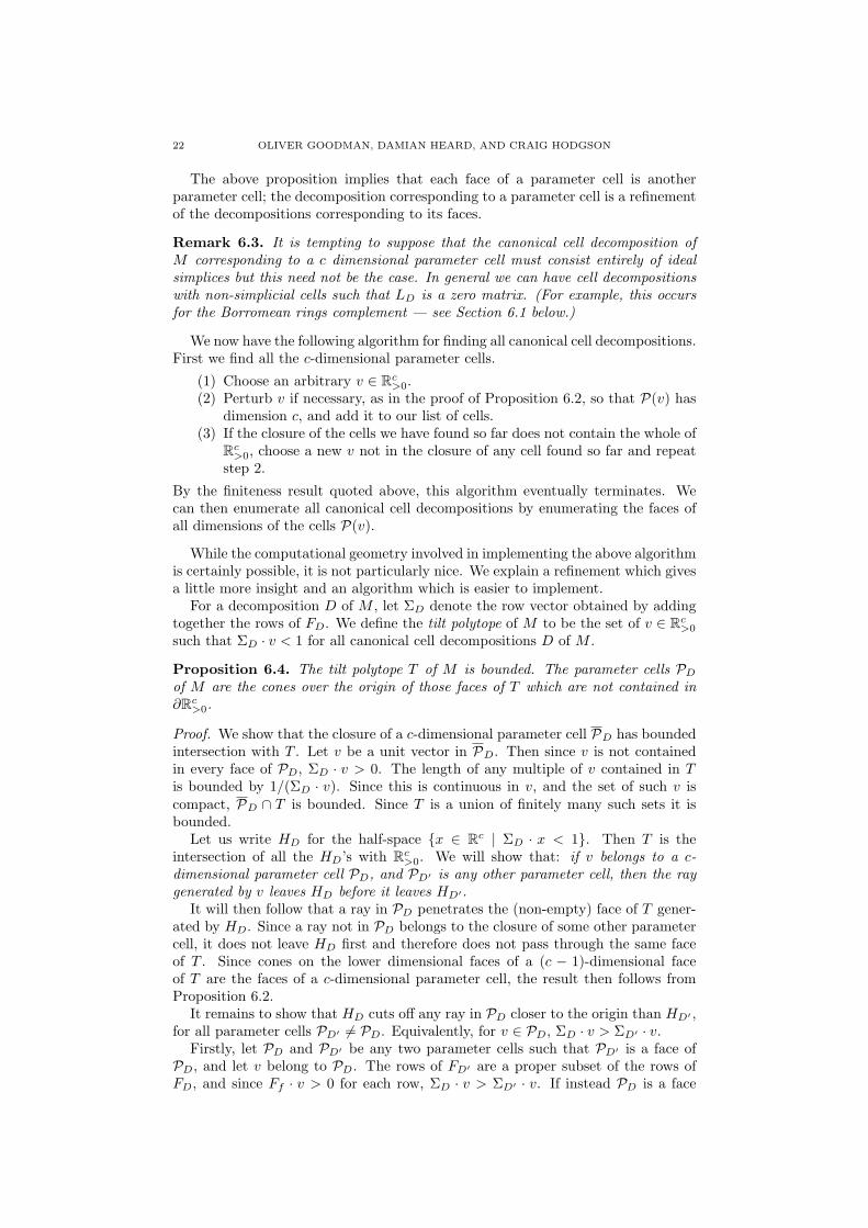
Let T0 be a polytope resulting from the intersection of Rc>0 with some of thehalf-spaces HD defined in the above proof. If T0 ) T , some face A = T 0 ∩ ∂HD
of T0 will contain a point v ∈ Rc>0 not in T , and thus not in T ∩ ∂HD, nor in thecone on this, PD. Therefore LDv 6= 0 or Ffv < 0 for some row Ff of FD. Thisgives a test for when T0 properly contains T ; when satisfied, it yields a new half-space HD(v) whose intersection with T0 is strictly smaller. After a finite number ofintersections we arrive at T0 = T . See Figure 5.
v
PD
w
T
T0
Figure 5. T0 is a partially computed tilt polytope. The face ofT0 containing v ∈ PD has a vertex w not in PD. Therefore D(w)gives another face of T .
The computational geometry involved in the above is relatively straightforward.By using homogeneous coordinates we can treat an unbounded region, such as Rc>0,as a polytope with some vertices “at infinity”. The face A of T0, as defined above,is the convex hull of those vertices v of T0 satisfying ΣD · v = 1. If any of thesesatisfy LDv 6= 0 or Ffv < 0 for some row Ff of FD we conclude that T0 6= T . Ifsuch v lies in ∂Rc>0 we perturb it a little to bring it inside Rc>0 before determininga new half-space HD(v).
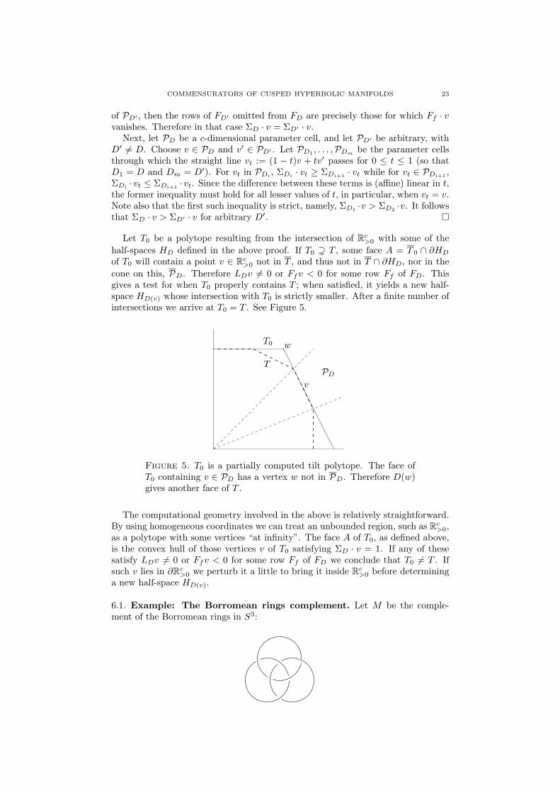
6.1. Example: The Borromean rings complement. Let M be the comple-ment of the Borromean rings in S3:
24 OLIVER GOODMAN, DAMIAN HEARD, AND CRAIG HODGSON
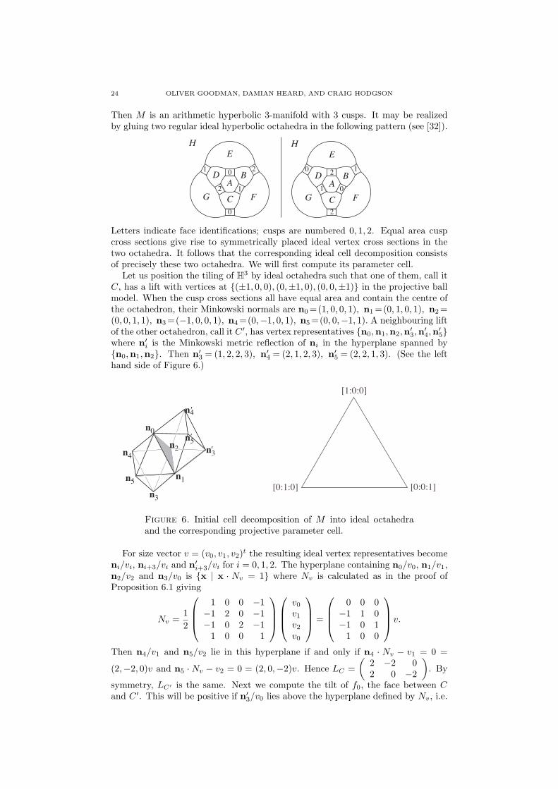
Then M is an arithmetic hyperbolic 3-manifold with 3 cusps. It may be realizedby gluing two regular ideal hyperbolic octahedra in the following pattern (see [32]).
HE
AD B
FCG
HE
AD B
FCG
0
2 1
1 2
0
2
1 0
0 1
2
Letters indicate face identifications; cusps are numbered 0, 1, 2. Equal area cuspcross sections give rise to symmetrically placed ideal vertex cross sections in thetwo octahedra. It follows that the corresponding ideal cell decomposition consistsof precisely these two octahedra. We will first compute its parameter cell.
Let us position the tiling of H3 by ideal octahedra such that one of them, call itC, has a lift with vertices at {(±1, 0, 0), (0,±1, 0), (0, 0,±1)} in the projective ballmodel. When the cusp cross sections all have equal area and contain the centre ofthe octahedron, their Minkowski normals are n0 =(1, 0, 0, 1), n1 =(0, 1, 0, 1), n2 =(0, 0, 1, 1), n3 =(−1, 0, 0, 1), n4 =(0,−1, 0, 1), n5 =(0, 0,−1, 1). A neighbouring liftof the other octahedron, call it C ′, has vertex representatives {n0,n1,n2,n′3,n
′4,n′5}
where n′i is the Minkowski metric reflection of ni in the hyperplane spanned by{n0,n1,n2}. Then n′3 = (1, 2, 2, 3), n′4 = (2, 1, 2, 3), n′5 = (2, 2, 1, 3). (See the lefthand side of Figure 6.)
n2
n0
n5
n4
n3
n1
n3
n5
n4′
′′
[1:0:0]
[0:1:0] [0:0:1]
Figure 6. Initial cell decomposition of M into ideal octahedraand the corresponding projective parameter cell.
For size vector v = (v0, v1, v2)t the resulting ideal vertex representatives becomeni/vi, ni+3/vi and n′i+3/vi for i = 0, 1, 2. The hyperplane containing n0/v0, n1/v1,n2/v2 and n3/v0 is {x | x · Nv = 1} where Nv is calculated as in the proof ofProposition 6.1 giving
Nv =12
1 0 0 −1−1 2 0 −1−1 0 2 −1
1 0 0 1
v0v1v2v0
=
0 0 0−1 1 0−1 0 1
1 0 0
v.
Then n4/v1 and n5/v2 lie in this hyperplane if and only if n4 · Nv − v1 = 0 =
(2,−2, 0)v and n5 ·Nv − v2 = 0 = (2, 0,−2)v. Hence LC =(
2 −2 02 0 −2
). By
symmetry, LC′ is the same. Next we compute the tilt of f0, the face between Cand C ′. This will be positive if n′3/v0 lies above the hyperplane defined by Nv, i.e.
COMMENSURATORS OF CUSPED HYPERBOLIC MANIFOLDS 25
if n′3 ·Nv − v0 = (−2, 2, 2)v > 0. Thus Ff0 = (−2, 2, 2), and the tilt is positive atv = (1, 1, 1)t. By symmetry, the other faces of the octahedra also have positive tilt.The parameter cell of this decomposition {v | v0 = v1 = v2} is, projectively, a point(as shown in the right half of Figure 6).
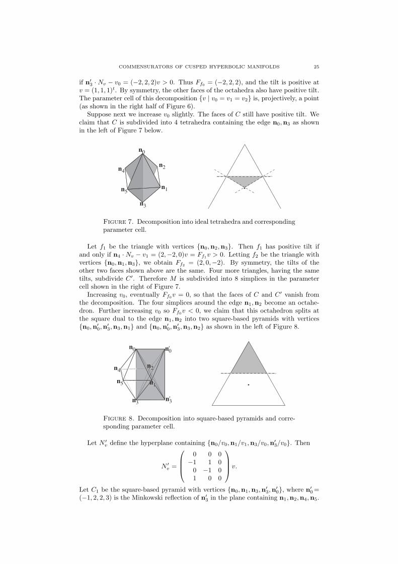
Suppose next we increase v0 slightly. The faces of C still have positive tilt. Weclaim that C is subdivided into 4 tetrahedra containing the edge n0,n3 as shownin the left of Figure 7 below.
n0
n5
n4
n3
n1
n2
Figure 7. Decomposition into ideal tetrahedra and correspondingparameter cell.
Let f1 be the triangle with vertices {n0,n2,n3}. Then f1 has positive tilt ifand only if n4 ·Nv − v1 = (2,−2, 0)v = Ff1v > 0. Letting f2 be the triangle withvertices {n0,n1,n3}, we obtain Ff2 = (2, 0,−2). By symmetry, the tilts of theother two faces shown above are the same. Four more triangles, having the sametilts, subdivide C ′. Therefore M is subdivided into 8 simplices in the parametercell shown in the right of Figure 7.
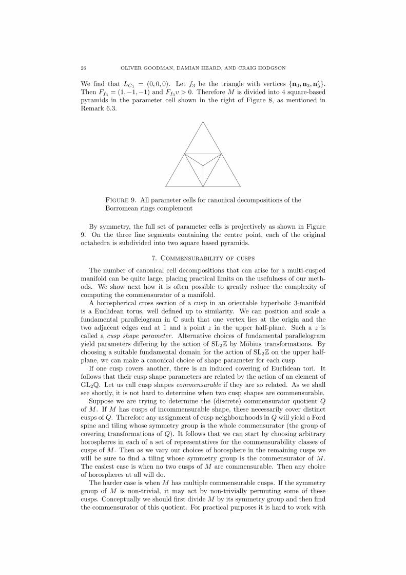
Increasing v0, eventually Ff0v = 0, so that the faces of C and C ′ vanish fromthe decomposition. The four simplices around the edge n1,n2 become an octahe-dron. Further increasing v0 so Ff0v < 0, we claim that this octahedron splits atthe square dual to the edge n1,n2 into two square-based pyramids with vertices{n0,n′0,n
′3,n3,n1} and {n0,n′0,n
′3,n3,n2} as shown in the left of Figure 8.
n2
n0
n5
n4
n3 n3′
n0′
n1
Figure 8. Decomposition into square-based pyramids and corre-sponding parameter cell.
Let N ′v define the hyperplane containing {n0/v0,n1/v1,n3/v0,n′3/v0}. Then
N ′v =
0 0 0−1 1 0
0 −1 01 0 0
v.
Let C1 be the square-based pyramid with vertices {n0,n1,n3,n′3,n′0}, where n′0 =
(−1, 2, 2, 3) is the Minkowski reflection of n′3 in the plane containing n1,n2,n4,n5.
26 OLIVER GOODMAN, DAMIAN HEARD, AND CRAIG HODGSON
We find that LC1 = (0, 0, 0). Let f3 be the triangle with vertices {n0,n3,n′3}.Then Ff3 = (1,−1,−1) and Ff3v > 0. Therefore M is divided into 4 square-basedpyramids in the parameter cell shown in the right of Figure 8, as mentioned inRemark 6.3.
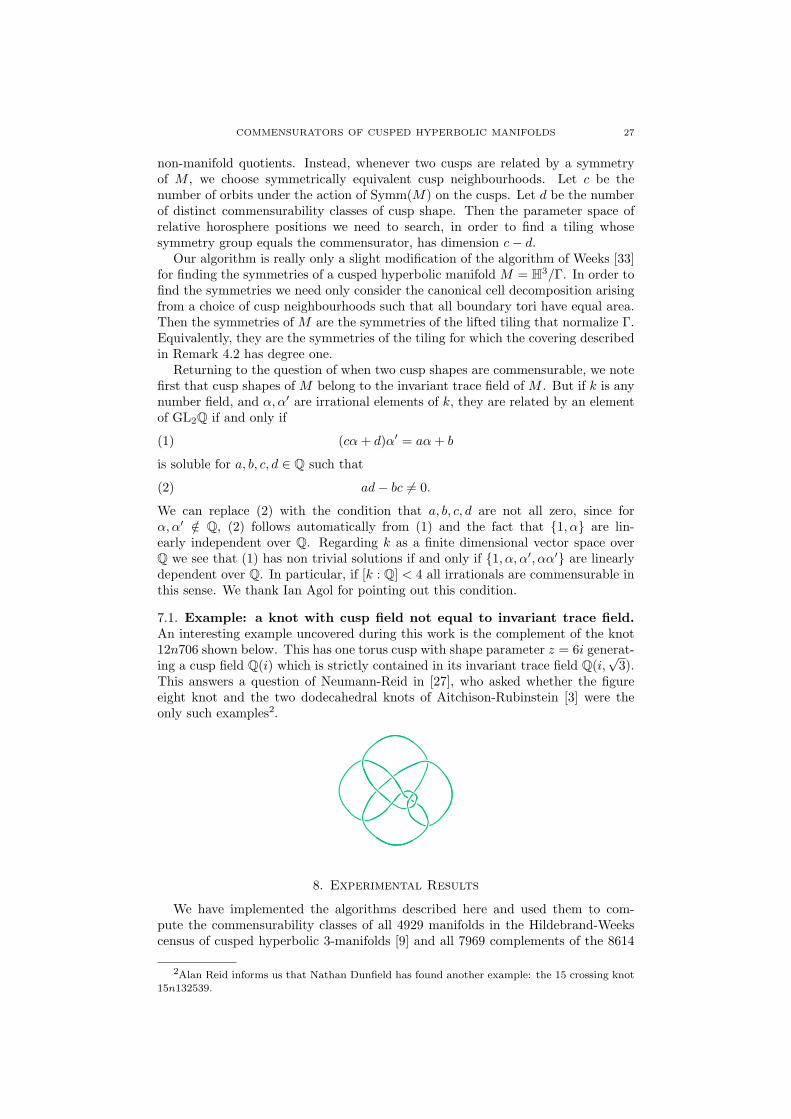
Figure 9. All parameter cells for canonical decompositions of theBorromean rings complement
By symmetry, the full set of parameter cells is projectively as shown in Figure9. On the three line segments containing the centre point, each of the originaloctahedra is subdivided into two square based pyramids.
7. Commensurability of cusps
The number of canonical cell decompositions that can arise for a multi-cuspedmanifold can be quite large, placing practical limits on the usefulness of our meth-ods. We show next how it is often possible to greatly reduce the complexity ofcomputing the commensurator of a manifold.
A horospherical cross section of a cusp in an orientable hyperbolic 3-manifoldis a Euclidean torus, well defined up to similarity. We can position and scale afundamental parallelogram in C such that one vertex lies at the origin and thetwo adjacent edges end at 1 and a point z in the upper half-plane. Such a z iscalled a cusp shape parameter. Alternative choices of fundamental parallelogramyield parameters differing by the action of SL2Z by Mobius transformations. Bychoosing a suitable fundamental domain for the action of SL2Z on the upper half-plane, we can make a canonical choice of shape parameter for each cusp.
If one cusp covers another, there is an induced covering of Euclidean tori. Itfollows that their cusp shape parameters are related by the action of an element ofGL2Q. Let us call cusp shapes commensurable if they are so related. As we shallsee shortly, it is not hard to determine when two cusp shapes are commensurable.
Suppose we are trying to determine the (discrete) commensurator quotient Qof M . If M has cusps of incommensurable shape, these necessarily cover distinctcusps of Q. Therefore any assignment of cusp neighbourhoods in Q will yield a Fordspine and tiling whose symmetry group is the whole commensurator (the group ofcovering transformations of Q). It follows that we can start by choosing arbitraryhorospheres in each of a set of representatives for the commensurability classes ofcusps of M . Then as we vary our choices of horosphere in the remaining cusps wewill be sure to find a tiling whose symmetry group is the commensurator of M .The easiest case is when no two cusps of M are commensurable. Then any choiceof horospheres at all will do.
The harder case is when M has multiple commensurable cusps. If the symmetrygroup of M is non-trivial, it may act by non-trivially permuting some of thesecusps. Conceptually we should first divide M by its symmetry group and then findthe commensurator of this quotient. For practical purposes it is hard to work with
COMMENSURATORS OF CUSPED HYPERBOLIC MANIFOLDS 27
non-manifold quotients. Instead, whenever two cusps are related by a symmetryof M , we choose symmetrically equivalent cusp neighbourhoods. Let c be thenumber of orbits under the action of Symm(M) on the cusps. Let d be the numberof distinct commensurability classes of cusp shape. Then the parameter space ofrelative horosphere positions we need to search, in order to find a tiling whosesymmetry group equals the commensurator, has dimension c− d.
Our algorithm is really only a slight modification of the algorithm of Weeks [33]for finding the symmetries of a cusped hyperbolic manifold M = H3/Γ. In order tofind the symmetries we need only consider the canonical cell decomposition arisingfrom a choice of cusp neighbourhoods such that all boundary tori have equal area.Then the symmetries of M are the symmetries of the lifted tiling that normalize Γ.Equivalently, they are the symmetries of the tiling for which the covering describedin Remark 4.2 has degree one.
Returning to the question of when two cusp shapes are commensurable, we notefirst that cusp shapes of M belong to the invariant trace field of M . But if k is anynumber field, and α, α′ are irrational elements of k, they are related by an elementof GL2Q if and only if
(1) (cα+ d)α′ = aα+ b
is soluble for a, b, c, d ∈ Q such that
(2) ad− bc 6= 0.
We can replace (2) with the condition that a, b, c, d are not all zero, since forα, α′ /∈ Q, (2) follows automatically from (1) and the fact that {1, α} are lin-early independent over Q. Regarding k as a finite dimensional vector space overQ we see that (1) has non trivial solutions if and only if {1, α, α′, αα′} are linearlydependent over Q. In particular, if [k : Q] < 4 all irrationals are commensurable inthis sense. We thank Ian Agol for pointing out this condition.
7.1. Example: a knot with cusp field not equal to invariant trace field.An interesting example uncovered during this work is the complement of the knot12n706 shown below. This has one torus cusp with shape parameter z = 6i generat-ing a cusp field Q(i) which is strictly contained in its invariant trace field Q(i,
√3).
This answers a question of Neumann-Reid in [27], who asked whether the figureeight knot and the two dodecahedral knots of Aitchison-Rubinstein [3] were theonly such examples2.
8. Experimental Results
We have implemented the algorithms described here and used them to com-pute the commensurability classes of all 4929 manifolds in the Hildebrand-Weekscensus of cusped hyperbolic 3-manifolds [9] and all 7969 complements of the 8614
2Alan Reid informs us that Nathan Dunfield has found another example: the 15 crossing knot15n132539.
28 OLIVER GOODMAN, DAMIAN HEARD, AND CRAIG HODGSON
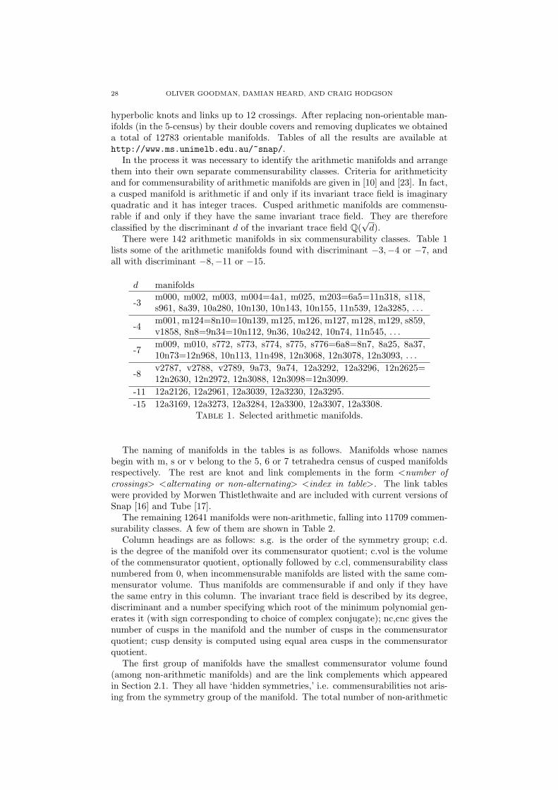
hyperbolic knots and links up to 12 crossings. After replacing non-orientable man-ifolds (in the 5-census) by their double covers and removing duplicates we obtaineda total of 12783 orientable manifolds. Tables of all the results are available athttp://www.ms.unimelb.edu.au/~snap/.
In the process it was necessary to identify the arithmetic manifolds and arrangethem into their own separate commensurability classes. Criteria for arithmeticityand for commensurability of arithmetic manifolds are given in [10] and [23]. In fact,a cusped manifold is arithmetic if and only if its invariant trace field is imaginaryquadratic and it has integer traces. Cusped arithmetic manifolds are commensu-rable if and only if they have the same invariant trace field. They are thereforeclassified by the discriminant d of the invariant trace field Q(
√d).
There were 142 arithmetic manifolds in six commensurability classes. Table 1lists some of the arithmetic manifolds found with discriminant −3,−4 or −7, andall with discriminant −8,−11 or −15.
d manifolds
-3m000, m002, m003, m004=4a1, m025, m203=6a5=11n318, s118,s961, 8a39, 10a280, 10n130, 10n143, 10n155, 11n539, 12a3285, . . .
-4m001, m124=8n10=10n139, m125, m126, m127, m128, m129, s859,v1858, 8n8=9n34=10n112, 9n36, 10a242, 10n74, 11n545, . . .
-7m009, m010, s772, s773, s774, s775, s776=6a8=8n7, 8a25, 8a37,10n73=12n968, 10n113, 11n498, 12n3068, 12n3078, 12n3093, . . .
-8v2787, v2788, v2789, 9a73, 9a74, 12a3292, 12a3296, 12n2625=12n2630, 12n2972, 12n3088, 12n3098=12n3099.
-11 12a2126, 12a2961, 12a3039, 12a3230, 12a3295.-15 12a3169, 12a3273, 12a3284, 12a3300, 12a3307, 12a3308.
Table 1. Selected arithmetic manifolds.
The naming of manifolds in the tables is as follows. Manifolds whose namesbegin with m, s or v belong to the 5, 6 or 7 tetrahedra census of cusped manifoldsrespectively. The rest are knot and link complements in the form <number ofcrossings> <alternating or non-alternating> <index in table>. The link tableswere provided by Morwen Thistlethwaite and are included with current versions ofSnap [16] and Tube [17].
The remaining 12641 manifolds were non-arithmetic, falling into 11709 commen-surability classes. A few of them are shown in Table 2.
Column headings are as follows: s.g. is the order of the symmetry group; c.d.is the degree of the manifold over its commensurator quotient; c.vol is the volumeof the commensurator quotient, optionally followed by c.cl, commensurability classnumbered from 0, when incommensurable manifolds are listed with the same com-mensurator volume. Thus manifolds are commensurable if and only if they havethe same entry in this column. The invariant trace field is described by its degree,discriminant and a number specifying which root of the minimum polynomial gen-erates it (with sign corresponding to choice of complex conjugate); nc,cnc gives thenumber of cusps in the manifold and the number of cusps in the commensuratorquotient; cusp density is computed using equal area cusps in the commensuratorquotient.
The first group of manifolds have the smallest commensurator volume found(among non-arithmetic manifolds) and are the link complements which appearedin Section 2.1. They all have ‘hidden symmetries,’ i.e. commensurabilities not aris-ing from the symmetry group of the manifold. The total number of non-arithmetic
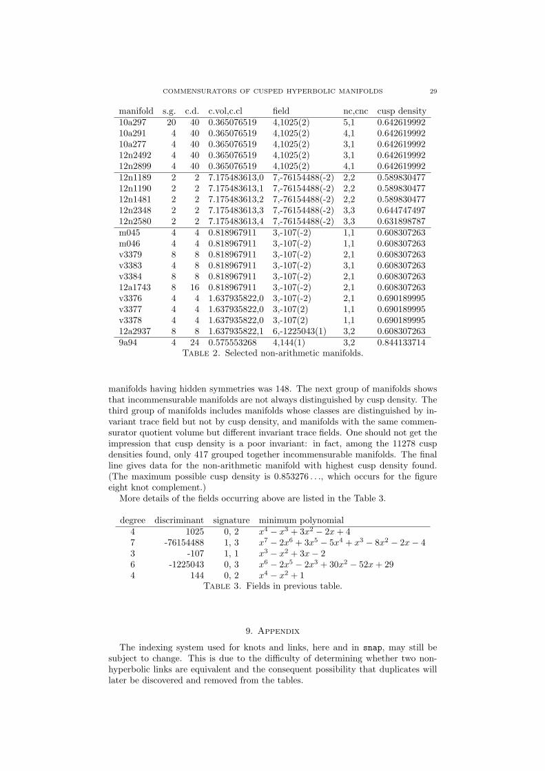
COMMENSURATORS OF CUSPED HYPERBOLIC MANIFOLDS 29
manifold s.g. c.d. c.vol,c.cl field nc,cnc cusp density10a297 20 40 0.365076519 4,1025(2) 5,1 0.64261999210a291 4 40 0.365076519 4,1025(2) 4,1 0.64261999210a277 4 40 0.365076519 4,1025(2) 3,1 0.64261999212n2492 4 40 0.365076519 4,1025(2) 3,1 0.64261999212n2899 4 40 0.365076519 4,1025(2) 4,1 0.64261999212n1189 2 2 7.175483613,0 7,-76154488(-2) 2,2 0.58983047712n1190 2 2 7.175483613,1 7,-76154488(-2) 2,2 0.58983047712n1481 2 2 7.175483613,2 7,-76154488(-2) 2,2 0.58983047712n2348 2 2 7.175483613,3 7,-76154488(-2) 3,3 0.64474749712n2580 2 2 7.175483613,4 7,-76154488(-2) 3,3 0.631898787m045 4 4 0.818967911 3,-107(-2) 1,1 0.608307263m046 4 4 0.818967911 3,-107(-2) 1,1 0.608307263v3379 8 8 0.818967911 3,-107(-2) 2,1 0.608307263v3383 4 8 0.818967911 3,-107(-2) 3,1 0.608307263v3384 8 8 0.818967911 3,-107(-2) 2,1 0.60830726312a1743 8 16 0.818967911 3,-107(-2) 2,1 0.608307263v3376 4 4 1.637935822,0 3,-107(-2) 2,1 0.690189995v3377 4 4 1.637935822,0 3,-107(2) 1,1 0.690189995v3378 4 4 1.637935822,0 3,-107(2) 1,1 0.69018999512a2937 8 8 1.637935822,1 6,-1225043(1) 3,2 0.6083072639a94 4 24 0.575553268 4,144(1) 3,2 0.844133714
Table 2. Selected non-arithmetic manifolds.
manifolds having hidden symmetries was 148. The next group of manifolds showsthat incommensurable manifolds are not always distinguished by cusp density. Thethird group of manifolds includes manifolds whose classes are distinguished by in-variant trace field but not by cusp density, and manifolds with the same commen-surator quotient volume but different invariant trace fields. One should not get theimpression that cusp density is a poor invariant: in fact, among the 11278 cuspdensities found, only 417 grouped together incommensurable manifolds. The finalline gives data for the non-arithmetic manifold with highest cusp density found.(The maximum possible cusp density is 0.853276 . . ., which occurs for the figureeight knot complement.)
More details of the fields occurring above are listed in the Table 3.
degree discriminant signature minimum polynomial4 1025 0, 2 x4 − x3 + 3x2 − 2x+ 47 -76154488 1, 3 x7 − 2x6 + 3x5 − 5x4 + x3 − 8x2 − 2x− 43 -107 1, 1 x3 − x2 + 3x− 26 -1225043 0, 3 x6 − 2x5 − 2x3 + 30x2 − 52x+ 294 144 0, 2 x4 − x2 + 1
Table 3. Fields in previous table.
9. Appendix
The indexing system used for knots and links, here and in snap, may still besubject to change. This is due to the difficulty of determining whether two non-hyperbolic links are equivalent and the consequent possibility that duplicates willlater be discovered and removed from the tables.
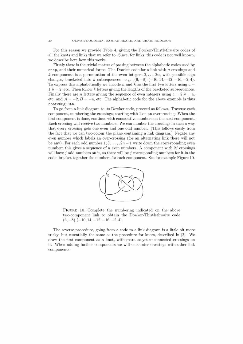
30 OLIVER GOODMAN, DAMIAN HEARD, AND CRAIG HODGSON
For this reason we provide Table 4, giving the Dowker-Thistlethwaite codes ofall the knots and links that we refer to. Since, for links, this code is not well known,we describe here how this works.
Firstly there is the trivial matter of passing between the alphabetic codes used bysnap, and their numerical forms. The Dowker code for a link with n crossings andk components is a permutation of the even integers 2, . . . , 2n, with possible signchanges, bracketed into k subsequences: e.g. (6,−8) (−10, 14,−12,−16,−2, 4).To express this alphabetically we encode n and k as the first two letters using a =1, b = 2, etc. Then follow k letters giving the lengths of the bracketed subsequences.Finally there are n letters giving the sequence of even integers using a = 2, b = 4,etc. and A = −2, B = −4, etc. The alphabetic code for the above example is thushbbfcDEgFHAb.
To go from a link diagram to its Dowker code, proceed as follows. Traverse eachcomponent, numbering the crossings, starting with 1 on an overcrossing. When thefirst component is done, continue with consecutive numbers on the next component.Each crossing will receive two numbers. We can number the crossings in such a waythat every crossing gets one even and one odd number. (This follows easily fromthe fact that we can two-colour the plane containing a link diagram.) Negate anyeven number which labels an over-crossing (for an alternating link there will notbe any). For each odd number 1, 3, . . . , , 2n− 1 write down the corresponding evennumber: this gives a sequence of n even numbers. A component with 2j crossingswill have j odd numbers on it, so there will be j corresponding numbers for it in thecode; bracket together the numbers for each component. See for example Figure 10.
−25 1
6
Figure 10. Complete the numbering indicated on the abovetwo-component link to obtain the Dowker-Thistlethwaite code(6,−8) (−10, 14,−12,−16,−2, 4).
The reverse procedure, going from a code to a link diagram is a little bit moretricky, but essentially the same as the procedure for knots, described in [2]. Wedraw the first component as a knot, with extra as-yet-unconnected crossings onit. When adding further components we will encounter crossings with other linkcomponents.
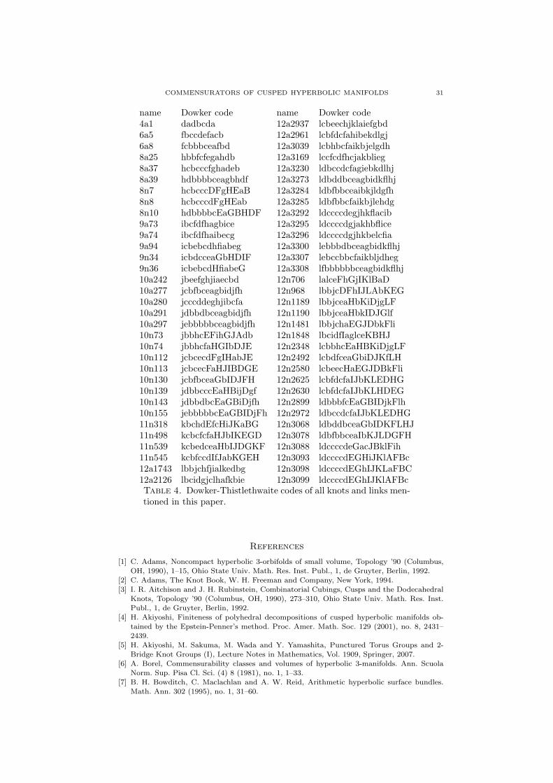
COMMENSURATORS OF CUSPED HYPERBOLIC MANIFOLDS 31
name Dowker code name Dowker code4a1 dadbcda 12a2937 lcbeechjklaiefgbd6a5 fbccdefacb 12a2961 lcbfdcfahibekdlgj6a8 fcbbbceafbd 12a3039 lcbhbcfaikbjelgdh8a25 hbbfcfegahdb 12a3169 lccfcdfhcjakblieg8a37 hcbcccfghadeb 12a3230 ldbccdcfagiebkdlhj8a39 hdbbbbceagbhdf 12a3273 ldbddbceagbidkflhj8n7 hcbcccDFgHEaB 12a3284 ldbfbbceaibkjldgfh8n8 hcbcccdFgHEab 12a3285 ldbfbbcfaikbjlehdg8n10 hdbbbbcEaGBHDF 12a3292 ldccccdegjhkflacib9a73 ibcfdfhagbice 12a3295 ldccccdgjakhbflice9a74 ibcfdfhaibecg 12a3296 ldccccdgjhkbelcfia9a94 icbebcdhfiabeg 12a3300 lebbbdbceagbidkflhj9n34 icbdcceaGbHDIF 12a3307 lebccbbcfaikbljdheg9n36 icbebcdHfiabeG 12a3308 lfbbbbbbceagbidkflhj10a242 jbeefghjiaecbd 12n706 lalceFhGjIKlBaD10a277 jcbfbceagbidjfh 12n968 lbbjcDFhIJLAbKEG10a280 jcccddeghjibcfa 12n1189 lbbjceaHbKiDjgLF10a291 jdbbdbceagbidjfh 12n1190 lbbjceaHbkIDJGlf10a297 jebbbbbceagbidjfh 12n1481 lbbjchaEGJDbkFli10n73 jbbhcEFihGJAdb 12n1848 lbcidfIaglceKBHJ10n74 jbbhcfaHGIbDJE 12n2348 lcbbhcEaHBKiDjgLF10n112 jcbcecdFgIHabJE 12n2492 lcbdfceaGbiDJKfLH10n113 jcbcecFaHJIBDGE 12n2580 lcbeecHaEGJDBkFli10n130 jcbfbceaGbIDJFH 12n2625 lcbfdcfaIJbKLEDHG10n139 jdbbcccEaHBijDgf 12n2630 lcbfdcfaIJbKLHDEG10n143 jdbbdbcEaGBiDjfh 12n2899 ldbbbfcEaGBIDjkFlh10n155 jebbbbbcEaGBIDjFh 12n2972 ldbccdcfaIJbKLEDHG11n318 kbchdEfcHiJKaBG 12n3068 ldbddbceaGbIDKFLHJ11n498 kcbcfcfaHJbIKEGD 12n3078 ldbfbbceaIbKJLDGFH11n539 kcbedceaHbIJDGKF 12n3088 ldccccdeGacJBklFih11n545 kcbfccdIfJabKGEH 12n3093 ldccccdEGHiJKlAFBc12a1743 lbbjchfjialkedbg 12n3098 ldccccdEGhIJKLaFBC12a2126 lbcidgjclhafkbie 12n3099 ldccccdEGhIJKlAFBcTable 4. Dowker-Thistlethwaite codes of all knots and links men-tioned in this paper.
References
[1] C. Adams, Noncompact hyperbolic 3-orbifolds of small volume, Topology ’90 (Columbus,OH, 1990), 1–15, Ohio State Univ. Math. Res. Inst. Publ., 1, de Gruyter, Berlin, 1992.
[2] C. Adams, The Knot Book, W. H. Freeman and Company, New York, 1994.
[3] I. R. Aitchison and J. H. Rubinstein, Combinatorial Cubings, Cusps and the DodecahedralKnots, Topology ’90 (Columbus, OH, 1990), 273–310, Ohio State Univ. Math. Res. Inst.
Publ., 1, de Gruyter, Berlin, 1992.[4] H. Akiyoshi, Finiteness of polyhedral decompositions of cusped hyperbolic manifolds ob-
tained by the Epstein-Penner’s method. Proc. Amer. Math. Soc. 129 (2001), no. 8, 2431–2439.
[5] H. Akiyoshi, M. Sakuma, M. Wada and Y. Yamashita, Punctured Torus Groups and 2-Bridge Knot Groups (I), Lecture Notes in Mathematics, Vol. 1909, Springer, 2007.
[6] A. Borel, Commensurability classes and volumes of hyperbolic 3-manifolds. Ann. ScuolaNorm. Sup. Pisa Cl. Sci. (4) 8 (1981), no. 1, 1–33.
[7] B. H. Bowditch, C. Maclachlan and A. W. Reid, Arithmetic hyperbolic surface bundles.Math. Ann. 302 (1995), no. 1, 31–60.
32 OLIVER GOODMAN, DAMIAN HEARD, AND CRAIG HODGSON
[8] J. O. Button, Fibred and virtually fibred hyperbolic 3-manifolds in the censuses. Experiment.
Math. 14 (2005), no. 2, 231–255.
[9] P. J. Callahan, M. V. Hildebrand and J. R. Weeks, A census of cusped hyperbolic 3-manifolds. (With microfiche supplement.) Math. Comp. 68 (1999), no. 225, 321–332.
[10] D. Coulson, O. Goodman, C. Hodgson and W. Neumann, Computing arithmetic invariantsof 3-manifolds, Experimental Mathematics 9 (2000), 127–152.
[11] D. B. A. Epstein and R. C. Penner, Euclidean decompositions of noncompact hyperbolic
manifolds. J. Differential Geom. 27 (1988), no. 1, 67–80.[12] W. Floyd and A. Hatcher, Incompressible surfaces in punctured-torus bundles. Topology
and its Applications 13 (1982), 263–282.
[13] F. Gonzalez-Acuna and W. C. Whitten, Imbeddings of three-manifold groups. Mem. Amer.Math. Soc. 99 (1992), no. 474, viii+55 pp.
[14] F. Gueritaud (with an appendix by D. Futer), On canonical triangulations of once-punctured
torus bundles and two-bridge link complements, Geometry and Topology 10 (2006), pp.1239-1284.
[15] F. Gueritaud, Geometrie hyperbolique effective et triangulations ideals canoniques en di-
mension 3, These de doctorat, Univ. Paris-sud, Orsay, 2006.[16] O. Goodman, Snap, the computer program, http://www.ms.unimelb.edu.au/˜snap/ and
http://sourceforge.net/projects/snap-pari.
[17] O. Goodman, Tube: a computer program for studying geodesics in hyperbolic 3-manifolds,available from http://www.ms.unimelb.edu.au/˜snap/.
[18] D. Heard, Orb: a computer program for studying hyperbolic 3-orbifolds, available fromhttp://www.ms.unimelb.edu.au/˜snap/orb.html.
[19] M. Hildebrand and J. Weeks, A computer generated census of cusped hyperbolic 3-manifolds.
Computers and mathematics (Cambridge, MA, 1989), 53–59, Springer, New York, 1989.[20] J. Hoste and M. Thistlethwaite, Knotscape, http://www.math.utk.edu/˜morwen/knotscape.html.
[21] M. Lackenby, The canonical decomposition of once-punctured torus bundles, Comment.
Math. Helv. 78 (2003) 363–384.[22] A. M. Macbeath, Commensurability of co-compact three-dimensional hyperbolic groups.
Duke Math. J. 50 (1983), no. 4, 1245–1253. Erratum: Duke Math. J. 56 (1988), no. 1, 219.
[23] C. Maclachlan and A. Reid, The arithmetic of hyperbolic 3-manifolds, Springer-Verlag, NewYork, 2003.
[24] G. A. Margulis, Discrete subgroups of semisimple Lie groups, Ergebnisse der Mathematik
und ihrer Grenzgebiete 17, Springer-Verlag, Berlin, 1991.[25] T. H. Marshall and G. J. Martin, Minimal Co-Volume Hyperbolic Lattices II, in preparation.
[26] R. Meyerhoff, The cusped hyperbolic 3-orbifold of minimal volume, Bull. Amer. Math. Soc.13 (1985), 154–156.
[27] W. D. Neumann and A. W. Reid, Arithmetic of Hyperbolic Manifolds, Topology ’90 (Colum-
bus, OH, 1990), 273–310, Ohio State Univ. Math. Res. Inst. Publ., 1, de Gruyter, Berlin,1992.
[28] W. D. Neumann and A. W. Reid, Notes on Adams’ small volume orbifolds, Topology ’90
(Columbus, OH, 1990), 311–314, Ohio State Univ. Math. Res. Inst. Publ., 1, de Gruyter,Berlin, 1992.
[29] A. W. Reid, A note on trace-fields of Kleinian groups. Bull. London Math. Soc. 22 (1990),
no. 4, 349–352.[30] M. Sakuma and J. Weeks, Examples of canonical decompositions of hyperbolic link comple-
ments. Japan. J. Math. (N.S.) 21 (1995), no. 2, 393–439.
[31] M. Sakuma and J. Weeks, The generalized tilt formula. Geom. Dedicata 55 (1995), no. 2,115–123.
[32] W. P. Thurston, The geometry and topology of three-manifolds, Princeton University Math.Dept. (1978). Also available at http://msri.org/publications/books/gt3m.
[33] J. R. Weeks, Convex hulls and isometries of cusped hyperbolic 3-manifolds. Topology Appl.52 (1993), no. 2, 127–149.
[34] J. Weeks, SnapPea, the computer program, available from
http://geometrygames.org/SnapPea/index.html.
[35] R. Zimmer, Ergodic theory and semi-simple Lie groups, Birkhauser, Boston, 1984.
Department of Mathematics and Statistics, University of Melbourne, Parkville, Vic-
toria 3010, Australia
E-mail address: [email protected], [email protected], [email protected]


![HARMONIC DEFORMATIONS OF HYPERBOLIC 3-MANIFOLDS … · The local rigidity theory of [21] was generalized by Bromberg ([8]) to include geometricallyfinite hyperbolic cone-manifolds](https://img.pdfslide.us/doc/110x75/5ffde1ae12ad7e6b4a3edebe/harmonic-deformations-of-hyperbolic-3-manifolds-the-local-rigidity-theory-of-21.jpg)


![Hyperbolic Manifolds - K. S. SARKARIA manifolds.pdf · 2016-03-27 · Hyperbolic Manifolds K. S. Sarkaria 1. Towards the end of [1] on pages 553-554 Sullivan sketched why closed [and](https://img.pdfslide.us/doc/110x75/5f143b2ab2479507162bdc46/hyperbolic-manifolds-k-s-sarkaria-manifoldspdf-2016-03-27-hyperbolic-manifolds.jpg)