Embed Size (px)
Citation preview
THE GENERATION AND APPLICATION OF METALLURGICAL
THERMODYNAMIC DATA
by
A. T. Dinsdale
Division of Materials Applications
National Physical Laboratory
Submitted for the degree of Doctor of Philosophy
at Brunel University, August 1984

ABSTRACT
The power of thermodynamics in the calculation of complex chemical
and metallurgical equilibria of importance to industry has, over the
last 15 years, been considerably enhanced by the availability of
computers. It has resulted in the storage of data in databanks, the use
of physical but complex models to represent thermodynamic data, the vast
effort spent in the generation of critically assessed data and the
development of sophisticated software for their application in
equilibrium calculations.
This thesis is concerned with the generation and application of
metallurgical thermodynamic data in which the computer plays a central
and essential role. A very wide range of topics have been covered from
the generation of data by experiment and critical assessment through to
the application of these data in calculations of importance to industry.
Particular emphasis is placed on the need for reliable models and
expressions which can represent the molar Gibbs energy as a function of
temperature and composition. In addition a new computer program is
described and used for the automatic calculation of phase diagrams for
binary systems. Measurements of the enthalpies of formation of alloys in
the Fe-Ti system are reported. All data for this system have been
critically assessed to provide a dataset consistent with the published
phase diagram. Critically assessed data for a number of binary alloy
systems have been combined in order to perform quantitative calculations
in two types of steel system. Firstly data for the Cr-Fe-Ni-Si-Ti system
have been used to provide information about the long term stability of
alloys used in fast breeder nuclear reactors. Secondly very complex
calculations involving nine elements have been made to predict the
distribution of carbon and various impurities between competing phases
in low alloy steels on the addition of Mischmetall. Finally a new model
is developed to represent the thermodynamic data for sulphide liquids
and is used in the critical assessment and calculation of data for the
Cu-Fe-Ni-S system. The phase diagram and thermodynamic data calculated
from the assessed data are in excellent agreement with those observed
experimentally.
The work reported in this thesis, whilst successful, has also
indicated areas which will benefit from further study particularly the
development of reliable data and models for pure elements, ordered solid
phases and liquid phases for high affinity systems.

CONTENTS
Page
CHAPTER 1 Introduction 1
CHAPTER 2 Sources of Data 6
CHAPTER 3 Representation of Thermodynamic Data 11
Molar Gibbs Energy 11
Temperature dependence 12
Concentration dependence 15
a) Ideal Solutions Model 15
b) Regular Solution Model 17
c) Quasi-Chemical Theory 21
d) Cluster Variation Method 23
e) Asymmetric Models 25
f) Empirical Representations 26
g) Extrapolation of Binary data into Multicomponent
Systems 27
h) Comparison between Geometrical Equations 31
i) Models for Solid 'Compound' Phases 32
j) Molten Salt Solutions 34
k) Metal Salt Systems 35
1) Silicate Systems 39
Summary 42
CHAPTER 4 The Role of the Computer in Thermodynamics 43
Introduction 43
Calculation of Equilibria 43
Critical Assessment of Data 48
Conclusions 50

Calculation of Phase Equilibria in the Ni-Fe-S system 109
Calculations in the Ni-Fe-Cu-S system
Conclusions
111
112
CHAPTER 9 Conclusions and Suggestions for Future Work 113
ACKNOWLEDGEMENTS
APPENDIX
REFERENCES

-1-
CHAPTER 1
Introduction
Any stranger to the field of thermodynamics must think it rather odd
that its application to industrial problems is still in a state of
hectic development. It is certainly true that the basic principles of
the subject are well established following the pioneering work of Gibbs
and others (1-6) towards the end of the last century. It is also true,
however, that in many fields of research considerable time may elapse
between the conception of a theory and its 'development to the stage
where it can be used to solve complex problems of practical interest. In
the case of thermodynamics, the initial definition of the principles led
to rapid growth in the amount of experimental work being performed. This
experimental work with its generation of vast quantities of data led
people to develop convenient mathematical expressions to link the data
together. This need for convenient but reliable mathematical formalisms
in turn led to greater emphasis being placed on a detailed understanding
of the underlying physics and consequently the development of more
fundamental theories.
As I hope to demonstrate in this thesis, thermodynamics is still at a
stage where it demands a high level of intellectual application in order
to provide the basis for the solution of important practical problems.
However with the birth of the age of computers a dramatic change is now
occurring which will allow a non-expert to solve complex problems
involving thermodynamics with very little effort. This is particularly
true of the area of metallurgical thermodynamics. The aim of this thesis
is to show how thermodynamic data for metallurgical systems can be
generated and used in conjunction with a computer to solve problems of
practical interest.
The importance and the use of thermodynamics are well known and this
b'f

-2-
is reflected in the growing number of conferences and journals devoted
to the subject. At NPL, there is a great tradition for conferences
devoted to thermodynamics (7-10). The latest of these conferences "The
Industrial Use of Thermochemical Data" (10) showed that, just within the
areas of metallurgy and inorganic chemistry, thermodynamics is being
used successfully in a wide range of industries for topics as diverse as
the development of materials for nuclear reactors (11-13), the
prediction of superalloys suitable for use in turbine blades (14,15),
the hydrometallurgical and pyrometallurgical extraction of metals from
minerals (14,16), the growth of crystals by vapour transport (17),
pollution control (18), steelmaking (19-23) and the development of
materials for lamp technology (24,25). It is probably true that even in
these areas, thermodynamics is not being used to its full potential.
One other aspect that stood out from this conference was the
breakdown of the delegates between government organisations,
universities and private industry. It was rather encouraging to note the
large representation of industry which may indicate that the scepticism
or even fear on the part of the industrial scientist in the use and
power of thermodynamics is disappearing.
There are many reasons for this sceptical attitude. The last time a
typical industrial scientist would have thought in detail about
thermodynamics would have been during his undergraduate days at
university. There he would have been confronted with an array of partial
differential equations, strange concepts such as reversible and
irreversible reactions, adiabatic and isothermal changes and the
escalation of entropy. All this might have seemed a long way from
solving a practical chemical or metallurgical problem. It is small
wonder that after a break of a few years he would view the prospect of
returning to thermodynamics with some trepidation. Even for those bold
enough to get past this stage, the problems have only just begun. The

-3-
non-expert must first find the data he needs for his calculations,
perhaps from the literature or standard compilations. However, can he be
sure that these data are reliable, sufficiently accurate and consistent
with each other and with the most recent experimental results? He may
also need to estimate some data which are not available or to
interpolate or extrapolate them well outside the range of their
measurement. Furthermore when all the data have been found or estimated,
the problems of interest are often so complex that they are impossible
to solve without resorting to a powerful computer. He may then need to
develop software so sophisticated that even the best intentioned
industrial scientist will feel thwarted in his attempts to use
thermodynamics to solve his problem.
However the application of thermodynamics is fast becoming painless
because of the expanding series of data compilations and computer
databanks, and the development of extremely general computer programs
for the calculations of complex equilibria. The problem therefore now
becomes one of making industry aware of what is available, and competent
and confident in its ability to use such tools. In the long run, much of
the responsibilty lies with the universities. They must provide
undergraduate teaching courses which are both relevant, showing just
what can be achieved by the use of thermodynamics, and up-to-date by
demonstrating the most recent techniques and facilities for solving
these problems painlessly, reliably and cost effectively.
There are a number of aspects of the application of thermodynamics
which must be covered in order to solve a particular problem and these
will be discussed in some detail in the next three chapters of this
thesis. In chapter 2, the question is considered of where it is possible
to find the data required for the calculations. Generally data for the
most important materials can be found in tabular form in books although
the opportunities offered by the computer now allow the storage and
- 14 -
retrieval of data as coefficients to an expression relating the
variation of the thermodynamic properties to the composition and
temperature. This is especially important for the more complex
equilibrium calculations which may require interpolation or
extrapolation of tabulated data. The formalisms commonly used are
described in Chapter 3.
Thermodynamic data are very versatile and can be used for the
calculation of equilibria for a wide range of systems and industrial
applications. Several different types of computer programs have been
developed and these have been reviewed in chapter 4 along with the other
applications of computers to the world of thermodynamics. As these
calculations become more and more important, so the need for reliable
and efficient procedures grows. Moreover as the power of computers
increases and their price drops these calculations fall well within the
scope of any interested individual. It now becomes important to develop
programs specifically for microcomputers. In chapter 5 the mathematics
and the strategy used for one particular computer program is described.
This program is used at NPL for the automatic calculation of binary
alloy phase diagrams. The techniques used for this program are very
reliable and so compact that they allow the calculation of phase
equilibria even on a hand held microcomputer.
Ultimately the basis of all the calculations of phase equilibria is
experimental work. In chapter 6a series of measurements are described
for the enthalpies of formation of alloys in the iron rich side of the
Fe-Ti system. This work involved the use of a high temperature adiabatic
calorimeter designed by Dench (26) but with experimental procedures
modified to allow measurements in highly exothermic systems such as the
Fe-Ti system. These experimental data, with thermodynamic and phase
diagram data from other sources were critically assessed in order to
provide a representation of the thermodynamic data over a wide range of
-5-
temperatures and compositions but consistent with the accepted phase
diagram.
In chapter 7 two sets of phase equilibrium calculations for steel
systems are described. The first set of calculations, which used a
database including the critically assessed data for the iron-titanium
system, was undertaken to provide reliable phase diagrams for
multicomponent stainless steels to help understand the phenomenon of
neutron induced void swelling of cladding materials used in fast breeder
nuclear reactors. These calculations are more reliable than could be
obtained from direct experiment because phase transformations in the
temperature range of interest are very sluggish in these systems. They
therefore give information about the long term stability of these
cladding alloys. The second set of calculations was designed to provide
quantitative information about the levels of Mischmetall which could be
added to certain low alloy steels to remove harmful impurities such as
phosphorus, tin and copper and yet would not cause a disruption of the
carbide structure of the steel.
In chapter 8 the assessment of thermodynamic and phase diagram data
for certain sulphide systems is described. These systems are
characterised by dramatic changes in the thermodynamic properties of the
liquid phase close to the compositions of known stoichiometric
compounds. A new model has been derived to represent the thermodynamic
data for the liquid phase as a function of temperature and composition.
In particular data have been derived for the Cu-S and Ni-S systems which
were then used to calculate the phase diagram and thermodynamic data for
the Cu-Fe-S, Cu-Ni-S, Fe-Ni-S and Cu-Fe-Ni-S system. These calculations
are in good agreement with available experimental information.
The final chapter, chapter 9, is a summary of the work carried out
for this thesis. Although the work has been successful a number of
aspects require further study and these have been highlighted.

-6-
CHAPTER 2
Sources of Data
One of the most difficult and important problems facing a potential
user of thermodynamics is to find the basic data needed to solve his
problem. This might involve the daunting task of searching through the
literature for thermodynamic data, equilibrium data and potentially
related measurements such as spectroscopic data. Even after a
comprehensive search and after the collection of the available data
there is no guarantee that he will have found all the data he requires.
He might then try to estimate those data that aren't available. The
estimation of data is a complex and time consuming task in its own right
and often requires many years of experience. Moreover he will have to
make some judgement about the validity of all the data he has collected
and ensure that they are all interconsistent. For many practical
problems he will also need to express the dependence of these
thermodynamic data on the temperature or composition. The choice of
expression is often far from simple especially for condensed solution
phases as described in Chapter 3.
Fortunately in response to the need for accurate and consistent
thermodynamic and phase diagram data, many governments and industries
have sponsored the preparation of various data compilations. In the past
this has included programmes to measure key unknown thermodynamic data.
Unfortunately these are generally labour intensive and recently they
have suffered greatly from the world recession and economic crisis.
Traditionally the compilations of thermodynamic and phase diagram data
have been in the form of hard copy publications and have been of immense
benefit to industry. For thermodynamic data the most useful general
publications have been the JANAF tables (27-31), those of Barin and
Knacke (32,33) and the IVTAN group (34-37), the NBS 270 series (38,39),
-7-
Medved'ev (40), and the CODATA publications (41,42), all of which have
been concerned primarily with data for pure substances or species. Other
publications such as Hultgren (43,44), Kubaschewski and Alcock (45),
Kaufman and Bernstein (46) and the CALPHAD journal (47) have covered
data for both pure substances and for solution phases. Data for dilute
solution in metals and alloys have also been tabulated (48-52). There
are also many comprehensive sources of phase diagrams and equilibrium
measurements of which the best known are undoubtedly Hansen and Anderko
and its supplements (53-55), Moffatt (56), Prince (57,58), Ageev (59),
Wisniak (60), the Pourbaix atlasses (61), 'The Phase Diagrams for
Ceramicists' (62), the Metals Handbook (63) and more recently the
Bulletin of Alloy Phase Diagrams (64).
These publications are generally easy to use and contain their
information in a form which can often be applied directly to the problem
of interest. Indeed so useful have they become that in many quarters
they are regarded as a sort of Bible. This dependence on individual
publications is also their main drawback. For example, many of the phase
diagrams presented in Hansen are now out of date many times over and yet
the phase diagrams it contains are used, often without any regard to
whether a more recent phase diagram is available. A more acute problem
can occur because of inconsistency between the tabulated thermodynamic
data obtained from different sources. Different compilations often refer
to different reference states and this can lead the unaware to obtain
completely incorrect results. Despite their undoubted use such
compilations should therefore be used with some caution.
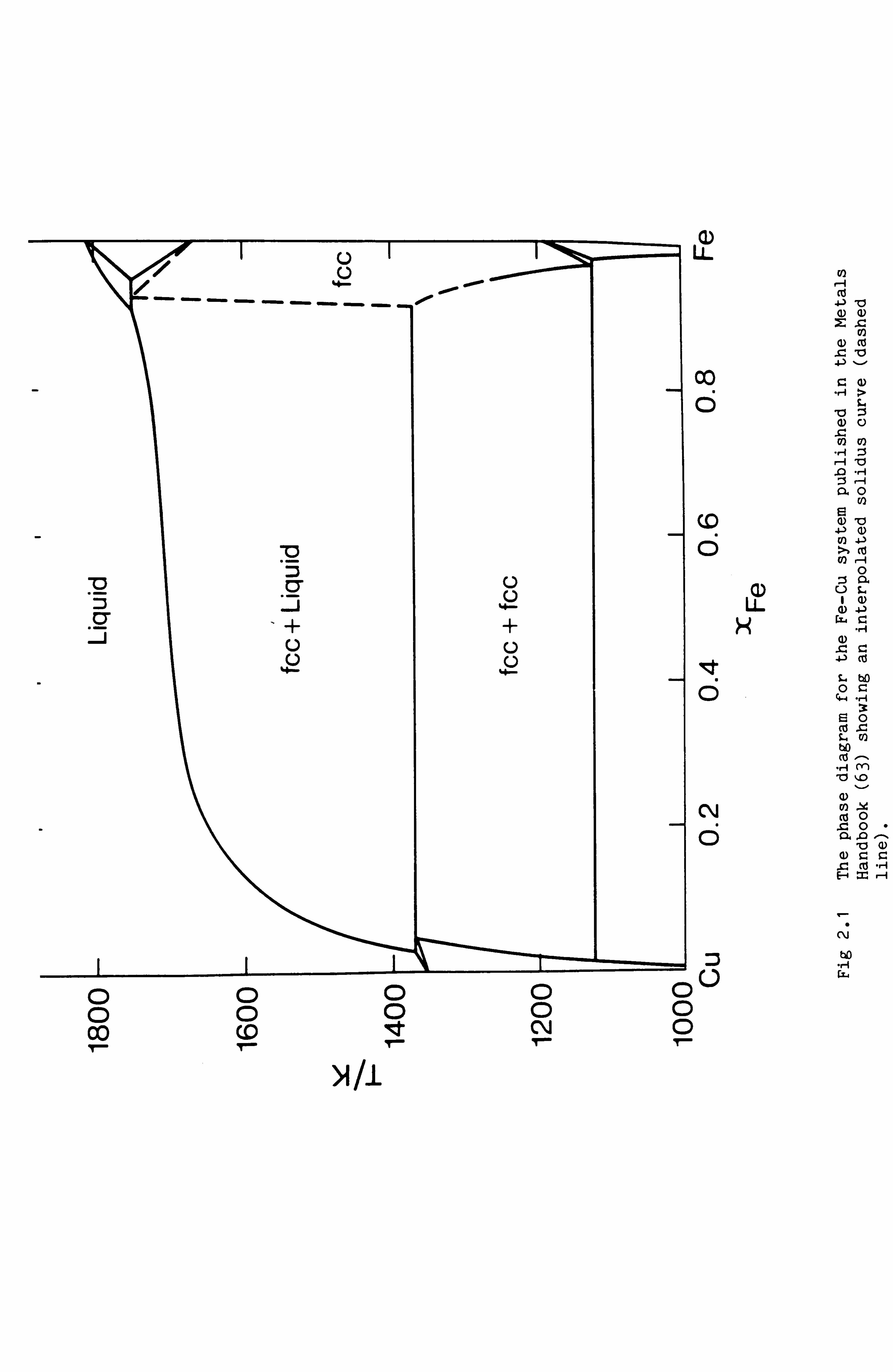
Moreover many of the published phase diagrams can be improved by
applying some simple knowledge of thermodynamics even without the use of
a computer. A good example of this has been demonstrated by Hillert
(65). In the phase diagram for the Fe-Cu system published in the Metals
Handbook (63) and reproduced in Fig 2.1, the phase boundary between the
QD LL
00
c5
c5
LL
H
0
N 6
U
>1/I
°0000 °00N0 rol r"
rr

-8-
Cu rich liquidus and the Fe rich fcc phase is represented by a dotted
line to indicate an editorial interpolation in the absence of specific
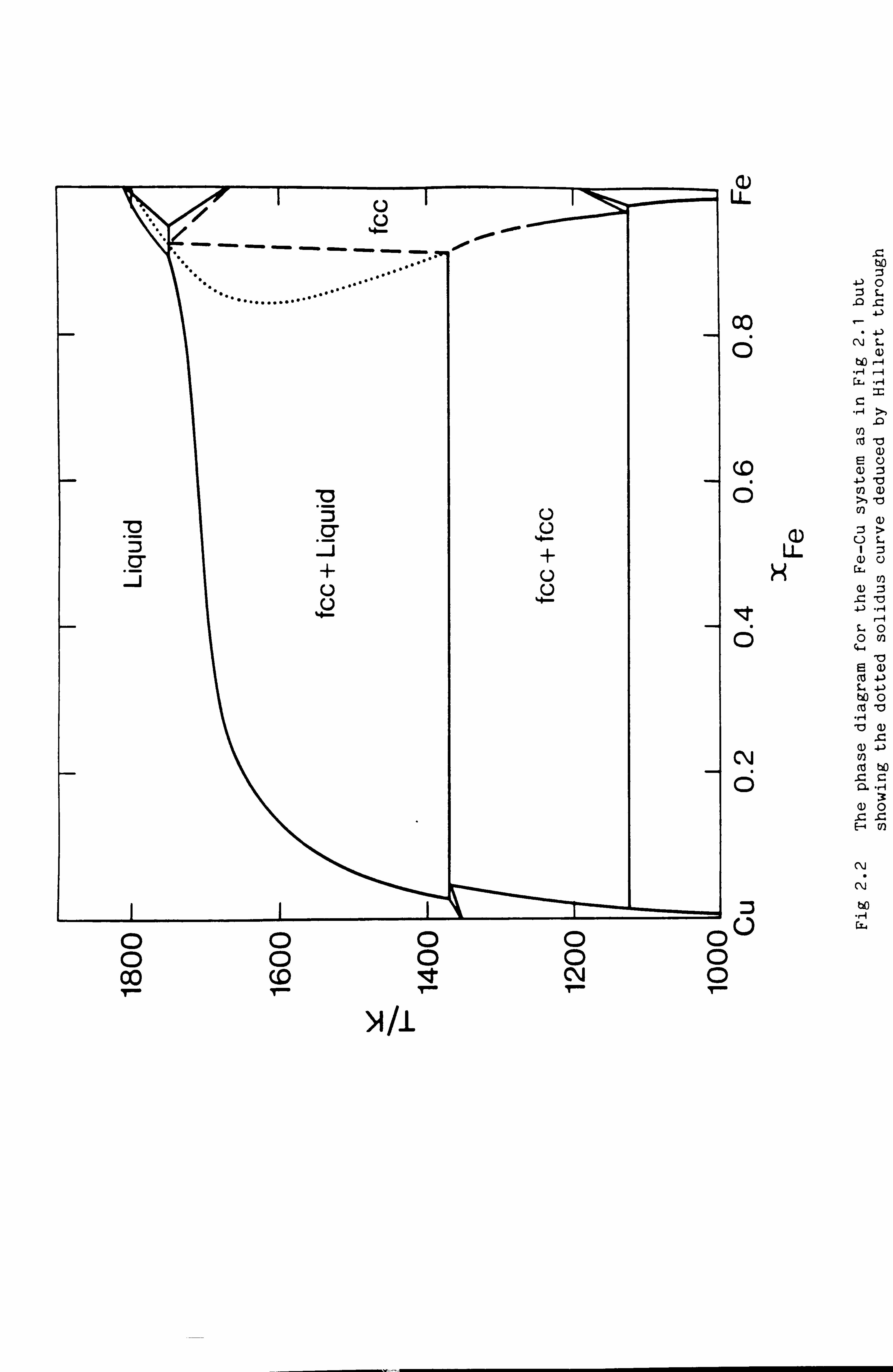
experimental results. Hillert (65) pointed out that the editor could
have defined this phase boundary more precisely. Firstly the two ends of
the dotted line indicate experimental compositions for which the fcc
phase is in equilibrium with the liquid phase. Also however the melting
point of metastable fcc Fe is known accurately from studies of a variety
of binary systems involving Fe where the fcc phase is stabilised (eg.
Fe-Ni). Hillert argued that the two ends of the dotted line and the
hypothetical melting point of fcc Fe, since they pertain to equilibrium
between the same two phases, should lie on a smooth curve as shown in
Fig 2.2. This has since been demonstrated experimentally.
In a similar way thermodynamics can be used very simply to examine
experimental liquidus and solidus curves in dilute solutions (66) and to
derive rules for the geometry of the intersections of phase boundaries
(67). Use of such knowledge in conjunction with experimental equilibrium
data can lead to more reliable phase diagrams.
Most of the compilations listed above are concerned with pure
substances or binary systems for perhaps alloys, aqueous solutions etc.
The number of tables or diagrams required for these systems is
sufficiently small that they can be stored in a few volumes.
Unfortunately, in practice, alloys or other materials of use to industry
rarely consist of only two elements and a source or compilation of phase
diagrams for complex materials is therefore sorely needed. Ageev (59) to
a certain extent fulfils this need for alloys. Recently The Metals
Society, in conjunction with SERC, has supported a project of work to
provide in hard copy form reviews of ternary phase diagrams for iron
based systems (68-72). Similarly Chang (73,74) has recently reviewed
selected ternary phase diagrams involving copper. However it is clearly
impossible to store phase diagrams for all multicomponent systems of
Ü ü
* CT + J U 42
U ý
U.
co
6
d
0
N O
o0000 CD 0 cc (0
0°000 TTTTT
a) LL
N/1

-9-
interest in hard copy form.
Fortunately there is a very close link between phase diagrams and
thermodynamic data. In fact it is correct to say that a phase diagram is
merely one of a number of different ways to represent the thermodynamic
data for a given system in a diagrammatic form. As the speed of
computers increases and reliable packages become available to calculate
phase diagrams from thermodynamic data (as described in Chapter 4) it
becomes tempting to replace hard copy data compilations by computer
databanks where the thermodynamic data are stored on computers in the
form of coefficients to some mathematical expression or expressions. The
quantity of data necessary to reproduce these hard copy compilations is
sufficiently small for them to be stored easily on a magnetic tape or
disc. Furthermore they will be self consistent, can be updated
frequently and accessed by people all over the world via a telephone
system or packet switching network. Perhaps more important the computer
will allow the calculation and presentation of results in any form
particularly appropriate to the user eg. a diagram could be plotted in
terms of weight percent rather than mole fraction.
Rather than produce hard copy data compilations the task now facing
professional thermodynamicists is to provide reliable, accurate and
consistent data for a wide variety of materials as a function of
temperature, composition and pressure. This in turn recognises the need
for reliable expressions to the represent the data and computer programs
both to assist in the generation of data and to calculate complex
equilibria.
This work is beyond the ability of one person or even one group of
people and has led to increased collaboration between different centres
throughout the world. One particularly effective forum for collaboration
is the CALPHAD organisation (CALculation of PHAse Diagrams) which
encourages free exchange of thermodynamic data. CALPHAD hosts a

- 10 -
conference every year at various centres throughout the world and a
journal, published quarterly, which acts as a focus for the development
of ideas, methods and data.
Within Europe a smaller organisation, SGTE (Scientific Group
Thermodata Europe), has been set up to provide European industries with
a source of reliable thermodynamic data and facilities for their use in
equilibrium calculations. A number of major European organisations
concerned with chemical and metallurgical data actively participate
including NPL, Harwell, RWTH Aachen, The Royal Institute of Technology
Stockholm, LTPCM and THERMODATA based in Grenoble and IRSID. One of its
main projects, which is sponsored in part by the EEC, is to set up a
computer based databank containing data for gases, alloys, oxide
systems, aqueous solutions, sulphides etc. and be capable of a wide
range of phase equilibrium calculations. It is planned to make this
databank available on-line to industry throughout the world from January
1986.
As will be described in chapter 4 similar databanks are being
developed in other parts of the world.
_. ý

- 11 -
CHAPTER 3
Representation of Thermodynamic Data
Molar Gibbs Energy
Of all the various types of data for materials, thermodynamic data
are probably the best suited for storage on a computer. One of the main
reasons for this is that a single function G, the molar Gibbs energy,
when expressed as a function of various system variables such as
temperature, pressure or composition, can be used to generate an
expression for any other thermodynamic property.
For example
Molar Volume V= (dG/8P) T
Molar entropy S=- (dG/dT)P
Molar enthalpy H=G-T (OG/d T)P
Internal energy U=G-T (a GIc T) P-P (d G/c)P) T
Helmholtz energy A=G-P (dG/dP)T
Specific heat at Cp =-T (d2G/c T2) P constant pressure
Specific heat at Cv - T(ä2G/c)T2)P - T(d2G/aTdP)2/(c)2G/JP2)T constant volume
Partial Gibbs energy GA =G-1 (dG18xA)y (1-x
A) i where yi =x and ii A
1-xA
Equally important from the point of view of the calculation of
chemical and metallurgical equilibria is that for a system to be in
thermodynamic equilibrium the Gibbs energy is at a minimum provided that
the system is homogeneous in temperature and pressure. Therefore for a
multiphase system the calculation of equilibria becomes a mathematical
I
- 12 -
problem of determining the phases and their compositions which, for a
given overall temperature and composition, give the lowest Gibbs energy.
For this it is essential that the Gibbs energies of all the competing
phases are represented as a single valued function of temperature,
pressure, composition and other appropriate variables. For practically
all problems of metallurgical interest this will be possible although
occasionally difficult. However for studies of critical phenomena
involving a liquid phase and a gas phase the Gibbs energy will no longer
be single valued. In this case it is more appropriate to use the
Helmholtz energy.
One handicap to the use of Gibbs energy is that it has no absolute
value - one can only discuss differences or changes in Gibbs energy.
Fortunately this is all that is necessary for the calculation of
equilibria.
Temperature dependence
For reliable calculations of phase equilibria it is very important to
use a good representation of the thermodynamic data as a function of
temperature even in regions where the phase is metastable. For most
materials where contributions to the thermodynamic properties arise from
electronic, vibrational and translational degrees of freedom the Gibbs
energy above 298.15 K can be conveniently and accurately represented by
an expression of the form:
G=a+bT+cT ln(T) +d T2 +e T3 +f T-1
and this is equivalent to the four term expression for Cp often used in
conjunction with some enthalpy and entropy values. Sometimes it is not
possible to represent data over a very wide temperature range using just
- 13 -
6 coefficients and in these conditions it is convenient to split the
temperature range into two or more intervals, each with a set of these 6
coefficients. The coefficients would normally be chosen such that there
was no discontinuity in the Gibbs energy, its first derivative or its
second derivative at the change from one temperature range to another.
There are however contributions to the thermodynamic properties which
for some substances can complicate the above treatment. The first occurs
for magnetic materials especially below and just above the Neel or Curie
temperature. Consider the case of Nickel which below 631 K is a
ferromagnet. We could choose to represent the thermodynamic data for
Nickel in two parts - firstly that for the paramagnetic form,
hypothetical at lower temperatures, which could be represented by the
conventional 6 term expression, and secondly a term for the magnetic
ordering. According to Inden (75,76) and Hillert and Jarl (77) this
magnetic contribution to the Gibbs energy will be given by:
Gmag =- RT 1n (P + 1),
where ß is the magnetic moment expressed as the number of Bohr
magnetons per atom, equivalent to twice the number of unpaired spins.
The function ý is different above and below the Curie temperature.
Above the Curie temperature
{ , r-5 + r- 15
+I -25 }/5K 2 63 300
Below the Curie temperature
-1 + 79 [ 'r -1 +2{ r3 + r9 7K 20 p 71 2 4-5
+ x'15 } {1 -1}1 200 p
where
- 14 -
518 + 11692 {1-1} 1125 15975 p
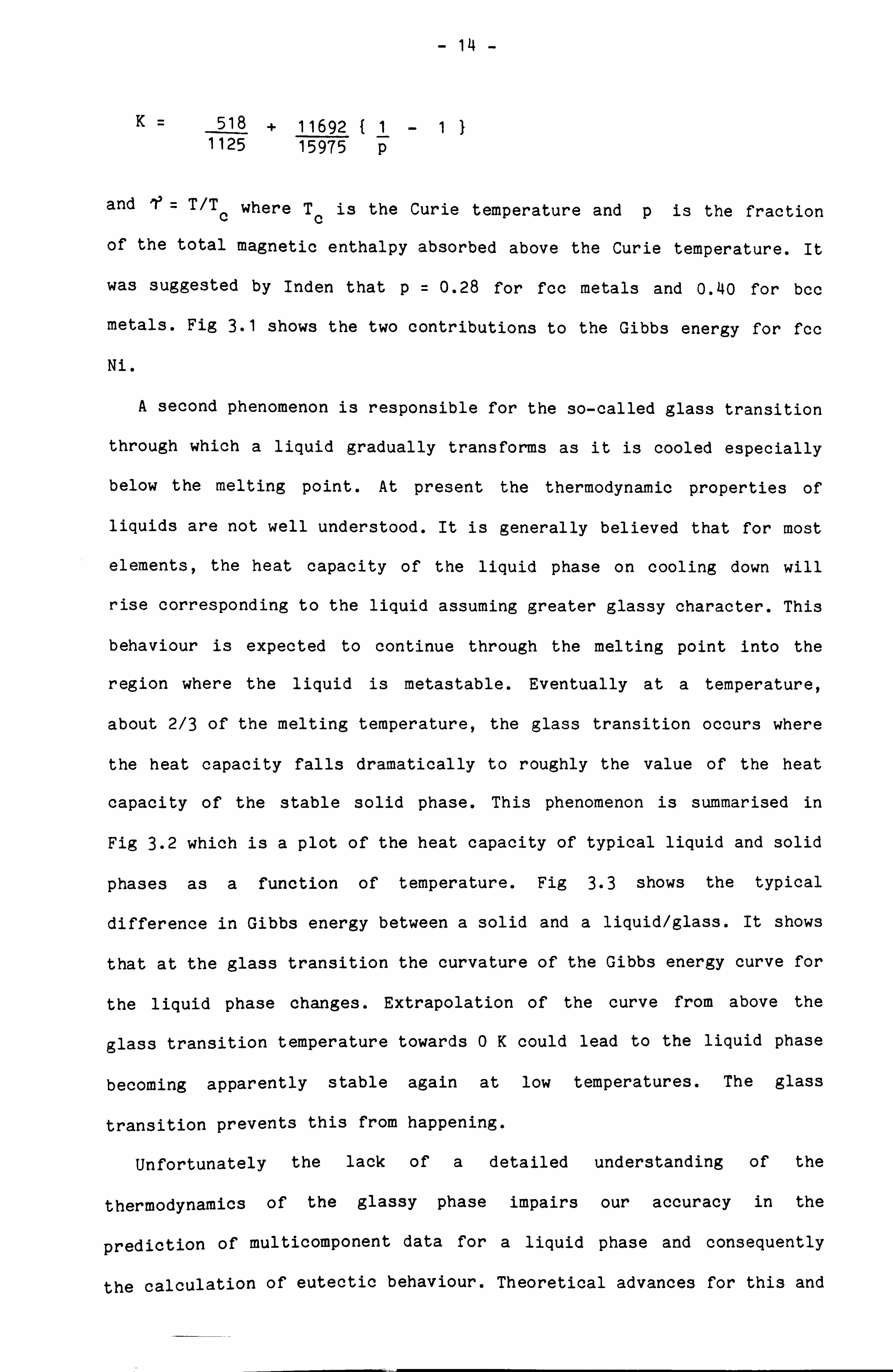
and l' = T/Tc where Tc is the Curie temperature and p is the fraction
of the total magnetic enthalpy absorbed above the Curie temperature. It
was suggested by Inden that p=0.28 for fcc metals and 0.40 for bcc
metals. Fig 3.1 shows the two contributions to the Gibbs energy for fcc
Ni.
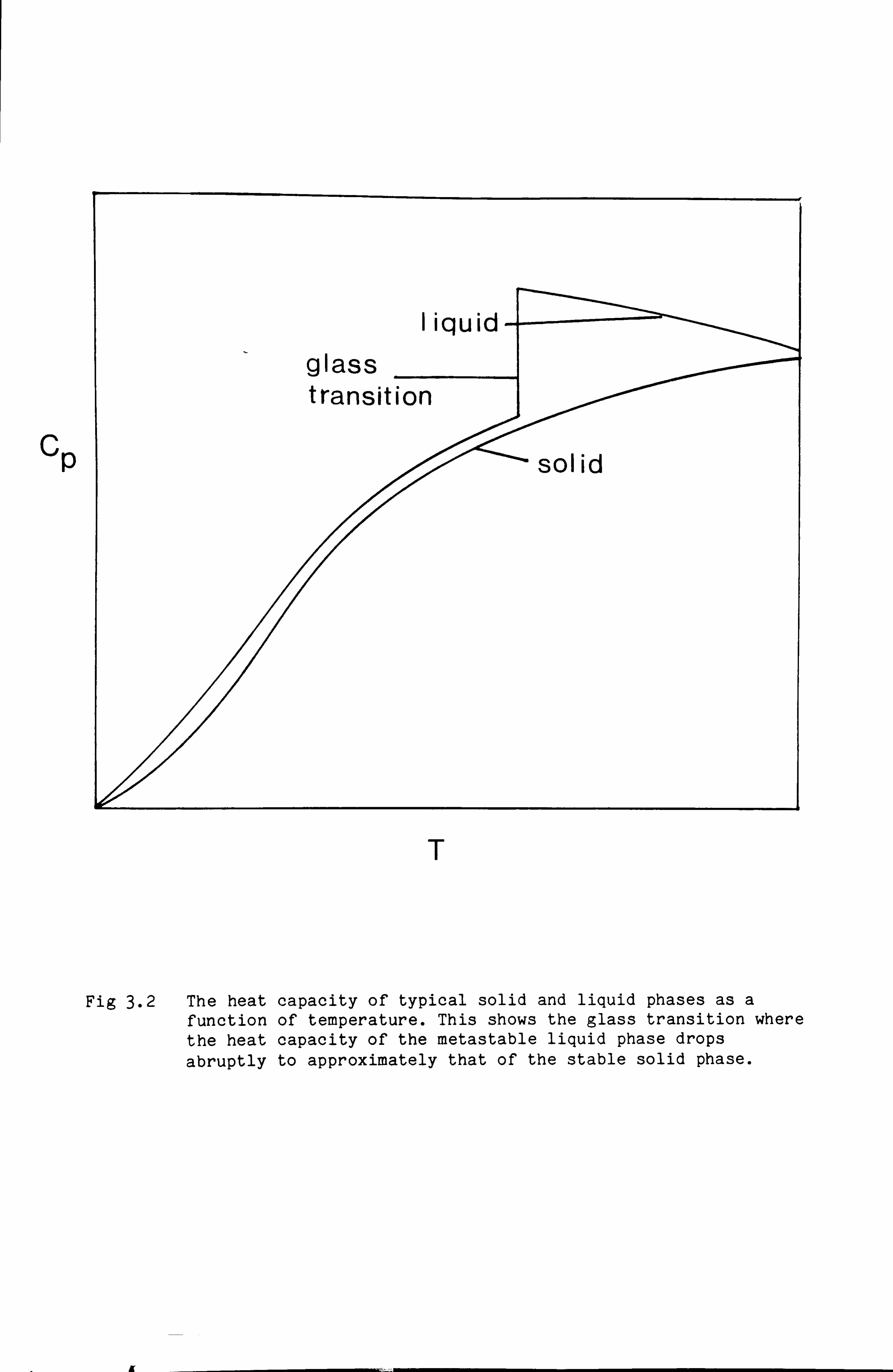
A second phenomenon is responsible for the so-called glass transition
through which a liquid gradually transforms as it is cooled especially
below the melting point. At present the thermodynamic properties of
liquids are not well understood. It is generally believed that for most
elements, the heat capacity of the liquid phase on cooling down will
rise corresponding to the liquid assuming greater glassy character. This
behaviour is expected to continue through the melting point into the
region where the liquid is metastable. Eventually at a temperature,
about 2/3 of the melting temperature, the glass transition occurs where
the heat capacity falls dramatically to roughly the value of the heat
capacity of the stable solid phase. This phenomenon is summarised in
Fig 3.2 which is a plot of the heat capacity of typical liquid and solid
phases as a function of temperature. Fig 3.3 shows the typical
difference in Gibbs energy between a solid and a liquid/glass. It shows
that at the glass transition the curvature of the Gibbs energy curve for
the liquid phase changes. Extrapolation of the curve from above the
glass transition temperature towards 0K could lead to the liquid phase
becoming apparently stable again at low temperatures. The glass
transition prevents this from happening.
Unfortunately the lack of a detailed understanding of the
thermodynamics of the glassy phase impairs our accuracy in the
prediction of multicomponent data for a liquid phase and consequently
the calculation of eutectic behaviour. Theoretical advances for this and
60
50
40
Cp 30 ýJ mol
K-'
20
10
total
paramagnetic
I,
fer ro - --"ýmagnet ic
1
300 500 700 900 1100 1300 1500 1700
T/ K
Fig 3.1 The heat capacity of nickel in the region of the Neel temperature showing the ferromagnetic and paramagnetic contributions.
`º I
liquid
glass transition
op solid
T
Fig 3.2 The heat capacity of typical solid and liquid phases as a function of temperature. This shows the glass transition where the heat capacity of the metastable liquid phase drops
abruptly to approximately that of the stable solid phase.

N 4.1
C vý "0 O N
cd . -I
b U) cd "r-1 G S.
ccS N va L a "r-+4-) e r1 a) cd cd 3 U r-1 O
ai. " N Cd 3O bO
cd
"ý O 3 ý
bo -P cd S-4 cd N Jzi as
N a) o'ý E
an 3 O .QO 0
"rl U) A
C' "r-4 rl "ý c :3
O U) U U" Cm N NN U) S. (f) cd
wc a wa r v
"o "r4
0 r4 H o') r-I
M
M
., 1 44
O L
Cl) 0
- 15 -
other phases of pure elements would be most welcome.
Concentration dependence
A great deal of work has been carried out into the development of
models and expressions to represent thermodynamic data for condensed
solution phases in binary systems and to extrapolate them into
multicomponent systems. Three general approaches have been adopted. The
most rigorous approach usually develops from the use of statistical
mechanics and an expression of the partition function from knowledge of
the various energy states available to the material. This in turn can be
related directly to the various thermodynamic functions.
An equivalent approach is to express the Gibbs energy in terms of
some internal variables of the system and then to find the conditions,
perhaps by numerical methods, which will give the lowest Gibbs energy of
the system.
The third approach, a more empirical one, is to adapt an essentially
theoretical model and use some power series expression to obtain good
agreement between the real behaviour and that predicted by the model.
This is the approach that is normally most useful and productive.
a) Ideal Solution Model
The most simple model is for a system where the elements involved
have very similar properties. Consider for example the liquid phase in a
system of two metals such as Co and Ni which are very similar in size,
are surrounded by the same number of nearest neighbour atoms and mix
together without any appreciable volume change or expulsion or
absorption of heat. Here it could be assumed that the metals would mix
together randomly and therefore form what is called an ideal solution.
- 16 -
In this case the thermodynamic properties of the solution can be
described fairly simply. Let us consider the Gibbs energy of formation
from the pure liquid elements of a composition in this liquid phase
where the mole fractions of Co and Ni are xCo and xNi respectively. For
an ideal solution, by definition, there is no enthalpy change on mixing.
However, there is an entropy contribution to the Gibbs energy because
the mixture has acquired some disorder. From the Boltzmann relationship
S=k 1n(SZ. )
where fL is the number of ways of arranging the system and k is the
Boltzmann constant. If the number of atoms per mole of the material is N
then kN = R. Therefore
S=k In { N! } (NxCo! )(NxNi)!
Applying Stirling's approximation
ln(z! ) =z ln(z)-z
S=-R{ xCo ln(xCo) + xNi ln(xNi) 1
The contribution of ideal mixing to the Gibbs energy therefore
= RT [xColn(xCo) + xNiln(xNi)]
Suppose now that the reference phases for pure nickel and cobalt are
not the liquid phase. In this case we must consider the transformation
of the pure metals from their reference phases to the liquid phase which
we can label by Goo and GNi respectively. The contribution from these
terms to the Gibbs energy of formation will be xCoGCo + XNiGNi'
Therefore the general expression for the Gibbs energy of formation for

- 17 -
such an ideal solution is given by:
tfG xCoG Co + xNiGNi + RT [xColn(xCo) + xNiln(xNi)]
and this expression could equally apply to any other phase such as fcc
or bcc.
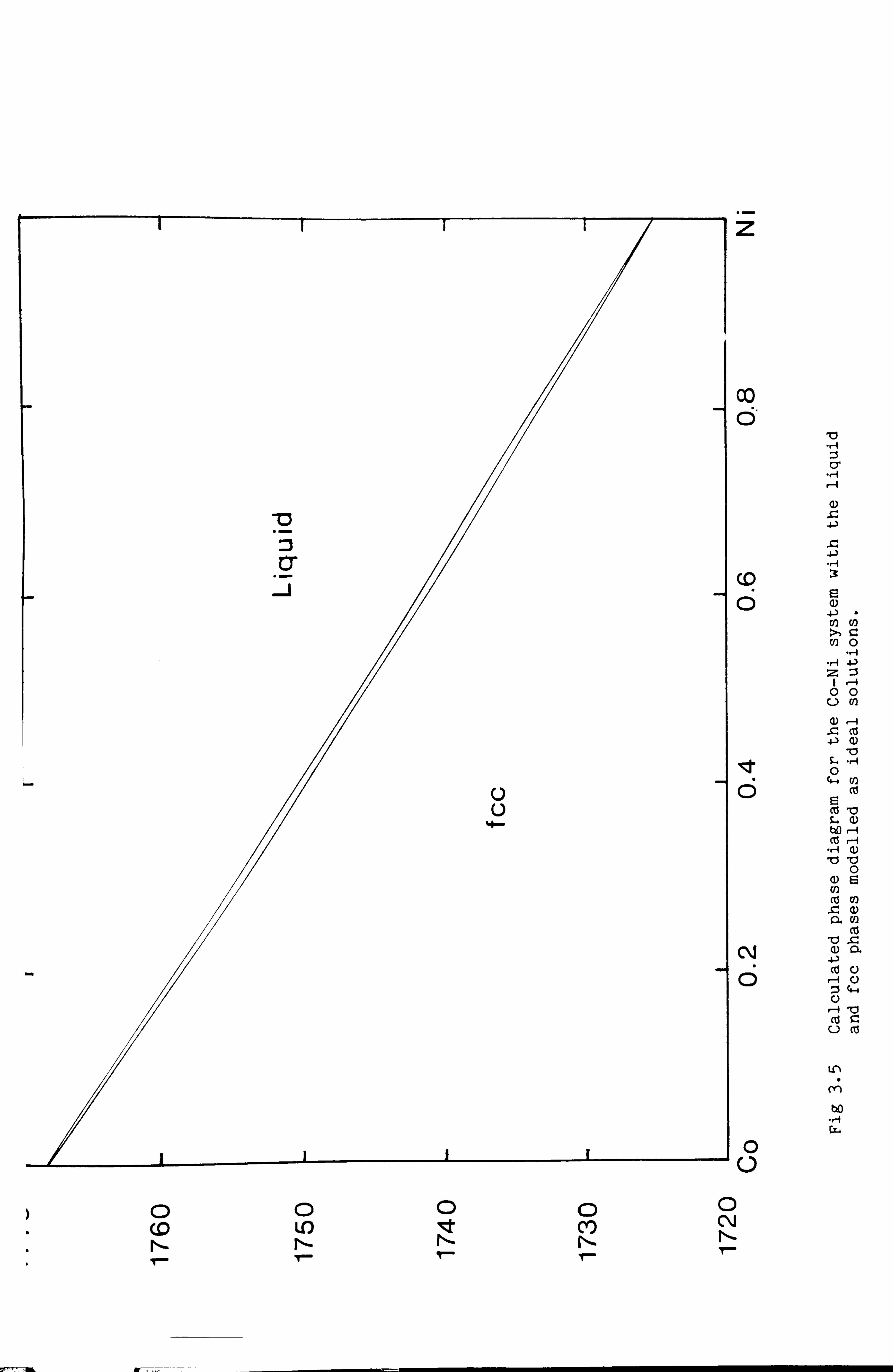
In Fig 3.4I we see a plot of the Gibbs energy for the liquid and fcc
phases at a temperature 1750 K as a function of composition. As is shown
in Chapter 4 the phase boundaries are given by the points of common
tangency to the two curves. If this procedure is performed for a number
of temperatures the phase diagram in Fig 3.5 is built up. This shows a
very simple lens type phase diagram in very good agreement with that
found from experiment.
Therefore for some materials a simple ideal solution model is able to
represent known thermodynamic and phase diagram data accurately. It can
easily be extended to any number of components in the solution to give
the equation
Aft = Xi Gi i=1
n +RT5 xi In xi
i=1
where n is the number of components and xi their concentrations. Gi is
the Gibbs energy of transformation from the pure component i in its
reference state to the phase in question at the temperature T.
b) Regular Solution Model
Solutions which exhibit ideal behaviour are rare and it is the norm
for components to show some kind of net interaction manifested either in
the form of a positive or negative enthalpy of mixing. This deviation
from ideality is called the excess Gibbs energy GE and it is the
expression of this as a function of composition that is the main focus

a
O Qý
-500
-1808
-1500
-2088
-2580
fcc
Iiquid
Co 0.28 0.48- 0.60 8.80 Ni
x -ý Ni
Fig 3.4 The Gibbs energies of formation for 1750 K of the liquid and fcc phases in the Co-Ni system modelled as ideal solutions
Z
00
o 'd
o'
r-4
a) 4)
E hi
N r-I .C cd
N 10
O Q
4-4 ri)
cd E cd 10 t. N b0 rl co r-I "r-4 a> bb
O NE Cl) C13 (1) .ZN am
C13 N a) a
cd rl
4-4 U
r-4 10 wc
0 cd
cn
.,. 4 Gc+
0 U
0 0 CD 00 NN CY) N
I` T
TT ý,

- 18 -
of theoretical and practical interest. The subject has been reviewed by
a number of authors, in particular by Oriani and Alcock (78), Ansara
(79,80) and Kapoor (81). The most basic approximation to represent the
excess Gibbs energy is the regular solution model.
The concept of regular solutions was introduced by Hildebrand (82-84)
from a study of the deviations of solubility curves from Raoult's law.
He found that "particularly among substances of low polarity, there
exist families of solubility curves which bespeak a marked regularity".
He called systems which were members of these families 'regular
solutions'. In order to explain this behaviour he adopted an approach of
Heitler (85,86) which considered a solution as a lattice and predicted
that the partial enthalpy of mixing should vary in an approximately
parabolic way. This formalism fitted Hildebrand's solubility data very
well.
The theory of regular solutions as developed by Hildebrand (82-84)
and Bragg and Williams (87) is such an important concept that it is
worth considering in some detail the theoretical background to the
model. Consider a mole of binary solution between two elements A and B.
As with the ideal solution model we can assume that the elements A and B
are of approximately the same size, are surrounded by the same number of
nearest neighbours, and mix together without any change in volume. Here
however we are considering a solution where there is an enthalpy change
on mixing arising from a net interaction between the elements. The bond
energy between two atoms should be short range and independent of the
other atoms they are bonded to. The total potential energy is then
assumed to be equal to the sum of contributions only from pairs of atoms
in direct contact. The most important assumption is that this
interaction between the atoms has no effect on the order of the solution
ie. the entropy of mixing is that for an ideal solution.
The total lattice energy of a solution having composition in mole

- 19 -
fraction terms (xA, xB) can be written as:
E nAAEAA f nABEAB + nBBEBB
where nAA' nAB and nBB are the number of bonds of the type A-A, A-B and
B-B respectively and EAA9 EAB and EBB are their respective energies. The
probability of finding an A atom and aB atom on a given site will be xA
and xB respectively. Therefore the probability of finding two chosen
adjacent sites occupied by two A atoms, two B atoms or one A atom and
one B atom will be xÄ, xB and 2xAxB respectively.
If we assume that all atoms in the solution have z nearest neighbours
the total number of bonds will be zN/2 where N is the number of atoms
per mole. We can now define the number of bonds of each type as its
probability of occurring multiplied by zN/2.
AA ie. n=zN xÄ n BB =zN xB n AB =zNxAB x
22
This leads us to the expression:
E_ zN EX2 + x2EBB + 2xAxBEAB] 2
The change in energy on alloying will be this quantity E minus lattice
energies for the pure elements which will be zNxAEAA/2 and zNxBEBB/2
respectively.
ie QE = -ZN [-xA(1-xA)EAA-xB(1-xB)EBB + 2xAxBEAB] 2
or, since xA + xB = 1,
E= ZN xAxB C2EAB-EAA-EBB1 =N xA xB w 2
xAxBL

- 20 -
where 2w/z is the energy required to change one AA pair and one BB pair
into two AB pairs, and L=Nw.
This quantity AE is equal to the enthalpy of mixing and therefore the
excess Gibbs energy since according to our initial assumptions the
volume change is zero and the mixing has been accompanied by no ordering
within the solution.
The expression for the excess Gibbs energy in the binary alloy case
can also be generalised for a multicomponent system through the same
procedure outlined above. Here one obtains
E n-1 n G= 7- 7 xi xi ij i=1 j=i+1
Consequently for systems obeying the regular solution assumptions the
thermodynamic data can be represented by one coefficient for each binary
system. Strictly this coefficient should be independent of temperature
although it has been the custom to relax this condition. Many binary and
ternary alloy systems 'have been represented successfully using the
regular solution model (88-90).
It is worth considering at this stage some of the implications of the
regular solution approximation for binary systems. Fig 3.6 shows typical
curves for the Gibbs energy of formation with different values of the
interaction parameter L. If L=0 we have an ideal solution as in curve
(a). If L is negative ie. there is a negative enthalpy of formation as
in curve (b), this is manifested by a Gibbs energy curve more negative
over all the composition range than for an ideal solution. If L is
positive, however, the ideal entropy term and the enthalpy of formation
term oppose one another and at certain temperatures will result in a
curve such as (c) with two distinct minima leading to a region where two
phases of the same structure are immiscible. For a regular solution a
positive interaction term will always lead to a miscibility gap for
r

lese
500
0
jII.
C
-500
-1000
-1508
-2000
-2500 b
a
A 0.20 0.40 0.60 0.80
x B
Fig 3.6 Curves for the Gibbs energies of formation of a phase modelled as a regular solution according to whether the interaction
parameter is 0 (ie. ideal solution, curve a), negative (curve b) or positive (curve c with two distinct minima leading to a region of immiscibility).
-3000
B

- 21 -
temperatures less than L/2R providing the phase is itself stable.
c) Quasi-Chemical Theory
The regular solution model has been criticised from a theoretical
point of view by Guggenheim (91) and Rushbrooke (92) because of its
assumption that even in systems with non-zero heats of mixing the atoms
will distribute themselves randomly among the lattice sites. In reality
the atoms will distribute themselves in order to reach the state with
the lowest Gibbs energy.
For the regular solution model, as shown earlier, the number of AB
bonds will be given by:
nAB =zN xA xB
If we let the number of A atoms be nA (= N xA) and the number of B atoms
be nB (= NxB) and rearrange we obtain
n2B = (z nA - nAB)(z nB - nAB)
Guggenheim and Rushbrooke (91-93) developed the Quasi-Chemical theory
to take into account the preferential distribution of various components
of the solution and these ideas were developed by Fowler (94,95) and
Bethe (96). From a rigorous treatment using statistical mechanics they
showed that:
n2 B nA - AB)(z nB - AB) e- 2w/zkT
From this equation one can see that if w=0 ie. for an ideal
solution we obtain the expression required for random mixing. If
however, 00 ie. an endothermic system, the formation of AB bonds will
_ ,;; Q,, r I1V' QPd and there will be a tendency to form AA and BB bonds and
IlL
- 22 -
for phase separation. If however w<O there will be a tendency for AB
pairs to form and ordering to occur.
The quantity znA - nAB is equal to 2n AA' twice the number of A-A
bonds in the mixture and similarly znB - nAB is equal to 2n BB, twice the
number of BB bonds in the mixture. Therefore for the quasi-chemical
theory:
2 nAB
nAAnBB e-2w/zkT
The similarity of this expression to the mass action law for chemical
reactions led to the adoption of the name 'quasi-chemical theory'.
The above expression can be solved for nAB or more appropriately x
= nAB/N given values for the other parameters.
ie. x= {1 +4 xA xB r}1/2 - 2
1 where ". e2w/zkT -
This expression can then be introduced into the statistical expression
for the excess Gibbs energy to give:
GE =RTz [xA 1n(xA - x) + xB 1n(xB - x) I 222
xA xB
This approach has been extended by Bonnier et al. (97) and Jena (98)
into ternary systems by solving iteratively equations of the form
xis _ (z xi - xij)(z x- xiJ) o(
where iij and d. ij
is given by:
pt ij
e- 2w ij
/kT

- 23 -
and incorporating into the expression
GE =RTzn n
2 i=1
where jii.
nY X-X
xi ln( j-1 1j
x2 i
Bonnier et al. applied this method to the Cd-Sn-Bi, Cd-Pb-Sn and
Cd-Pb-Bi systems. A numerical approach was also adopted by Stringfellow
and Greene (99,100) for the calculation of the phase diagrams for the
In-Ga-As, In-As-Sb, Ge-Si-Sn and Ge-Si-Pb systems.
For cases where the net interactions between atoms or molecules are
small an alternative approach can be adopted. As an example, for binary
systems the expression for x can be expanded as a power series in xAxB ll
and then expanded again by expressing T as a power series in terms of
2w/zkT which on omitting the higher order terms gives
GE = xA xB L[1- xA xB z2RLT]
which was been adopted by Kleppa (101) in his study of the Sn-Au system.
Hagemark (102,103) and Wagner (104) have derived analytical
expressions for the thermodynamic properties of multicomponent systems
using the quasi-chemical approximation.
d) Cluster Variation Method
The regular solution model discussed earlier takes its basic building
block to be lattice points which interact with their neighbours. The
quasi-chemical theory discussed in the last section is based around
pairs of atoms but as shown by Guggenheim (93) this is still an
approximation. In a generalisation of Bethe's procedure he showed that

- 24 -
even better approximations could be obtained by considering triangular
triplets or tetrahedral quadruplets and this was used by Li (105) to
explain ordering phenomena in fcc binary alloys. Unfortunately larger
clusters lead to greater numerical problems.
Takagi (106) adopted a different procedure from the quasi chemical
theory but still using pairs of atoms as the basic building block and
derived essentially the same expression. From a generalisation of
Takagi's approach Kikuchi, in a series of papers (107-115) developed the
Cluster Variation method. According to this method the Gibbs energy is
described in terms of a set of variables derived from a predefined
cluster of atoms. Instead of forming the partition function as used for
the quasi-chemical theory, the Gibbs energy is minimised with respect to
these variables in order to find the most stable atomic arrangement. The
smallest cluster possible is a lattice point from the Bragg-Williams'
approximation and the cluster variation method reproduces the regular
solution model. The next most complicated cluster is a pair of atoms,
and as demonstrated by Takagi, this gives results identical to the
quasi-chemical theory. For higher order clusters, represented in the
Cluster Variation model as extensions of these smaller clusters, the
method gives more accurate results than the quasi-chemical model. For
example a tetrahedon cluster variation approximation has been applied by
van Baal to fcc binary alloys (116) giving different and more accurate
results than those of Li (105).
To date the cluster variation method has been used mainly with
considerable success for the study of ordering reactions in alloy
systems using one parameter for the pairwise interaction between two
elements. Recently Kikuchi has used the method to calculate the phase
diagrams of the In-Ga-As and In-Sb-As systems, previously studied by
Stringfellow and Greene using the quasi-chemical approximation. He
obtained good agreement with their calculations and with experimental
- 25 -
data.
More recently Kikuchi (115) has attempted to derive data for the
Hg-Te and Cd-Te systems to be consistent with the observed liquidus
measurements. He used essentially an associated solution model (see
later) with species of HgTe and CdTe with their interactions represented
by a pair approximation of the cluster variation model.
e) Asymmetric Models
Unfortunately all the models discussed so far suffer from the same
basic drawback in that one parameter is rarely sufficient to represent
the thermodynamic data for typical binary alloy systems. This is not
surprising since one would expect that the bond energy between say an A
atom and aB atom might be dependent on their environments. Similarly
other factors such as the relative sizes of A and B and electronic
effects cannot usually be represented by just one parameter
(46,117-119).
A number of different attempts have been made to solve this problem.
Hardy (120) introduced a so-called subregular solution model when he
assumed that the interaction coefficient L could be represented as a
function of composition
ie. GE =xAxB (L1 xA + L2xB)
Kaufman has also used the subregular model but as an extension he
represented the coefficients L1 and L2 as functions of temperature (46).
Sharkey et al. (121) derived an expression based upon the
quasi-chemical theory which incorporates composition dependence in the
form:
22 I 0ý-, XQ XB f C2XA Xg - XA XB
- 26 -
and applied this to a large number of binary alloy systems. They also
proposed an extrapolation into ternary systems using a ternary
interaction term and applied their formalism with some success to the
Bi-Cd-Pb, Cd-Pb-Sn and Cd-Pb-Sb systems.
Another model which allows the interpretation of asymmetric data for
binary systems is the Central or Surrounded Atom model. This model was
suggested simultaneously by Lupis and Elliott (122) and Mathieu et al.
(123-125). Rather than concentrating on bonds, this model considers the
effect on individual atoms in the field of force of its nearest
neighbours.
Here the bonding energy between two atoms is no longer assumed to be
independent of its surroundings. Furthermore vibrational contributions
to the thermodynamic properties of mixing, neglected in previous models
were introduced. Normally an empirical function was used to represent
the changes in bond energy or vibrational parameters with changes in the
composition of the nearest neighbour environment although a linear or
parabolic function has generally been used. _
The surrounded atom model has been extended into ternary system by
Brion et al. (126,127). For simplicity the Bragg-Williams' statistics
are usually applied giving a quasi-regular solution model. According to
Ansara (79) the application of the Bethe statistics as used for the
quasi-chemical theory requires unreasonable computing time.
f) Empirical Representations
The theoretical approach adopted hitherto has had great success in
describing complex phenomena such as ordering. However in most binary
alloy systems, the physical interactions are too complicated to be
represented simply by one or two parameters. It is then necessary to use
sk
- 27 -
an empirical extension of the theoretical approach. The most widely used
representation is a power series expression.
There is nothing new about the use of power series expressions - one
form was used by Margules (128,129) in the last century. However the
advent of digital computers and data fitting techniques have made the
use of power series expressions practicable. A number of expressions
have been suggested eg. by Guggenheim (130), Wohl (131), Carlson and
Colburn (132), Benedict et al. (133) and Bale and Pelton (134) who also
advocated the use of Legendre polynomials (135). Other formalisms have
been suggested by Krupkowski (136), Esdaile (137) and Wilson (138).
However the most useful form was suggested by Redlich and Kister
(139,140).
GE = xAxB(Lo + L1 (xA-xB) + L2(xA-xB)2 + L3(xA-xB)3 .................. )
g) Extrapolation of binary data into Multicomponent Systems
The extension of the regular solution model into a multicomponent
system is straightforward as was shown earlier. For binary data
represented by more complex expressions there is no longer a unique way
of carrying out this extrapolation. Several different approaches have
been suggested for use usually in terms of some geometrical model where
the multicomponent excess Gibbs energy is calculated as a weighted sum
of excess Gibbs energies of certain defined binary compositions. These
are shown in Fig 3.7 and will now be discussed in turn.
Bonnier equation
According to the Bonnier equation (141) the excess Gibbs energy derived
from the composition path shown in Fig 3.7a is given by
- 28 -
GE xB x
GAB(xA, 1-xA) +ý GAC (xA, 1-xA) 1-xA 1-xA
+ (1-xA) GBC ( xB xC
) xB+xC xB+xC
where for example the term GAB(xA, 1-xA) refers to the excess Gibbs
energy of a composition in the binary system AB with the composition of
element A equal to xA and that of B equal to 1-x A* Spencer et al. (142) showed that this equation orginates from the
summation of three terms, the formation of the two binary compositions
in the AB and AC binaries weighted according to the overall composition
followed by a mixing of the two binary compositions using the data for
the binary system BC.
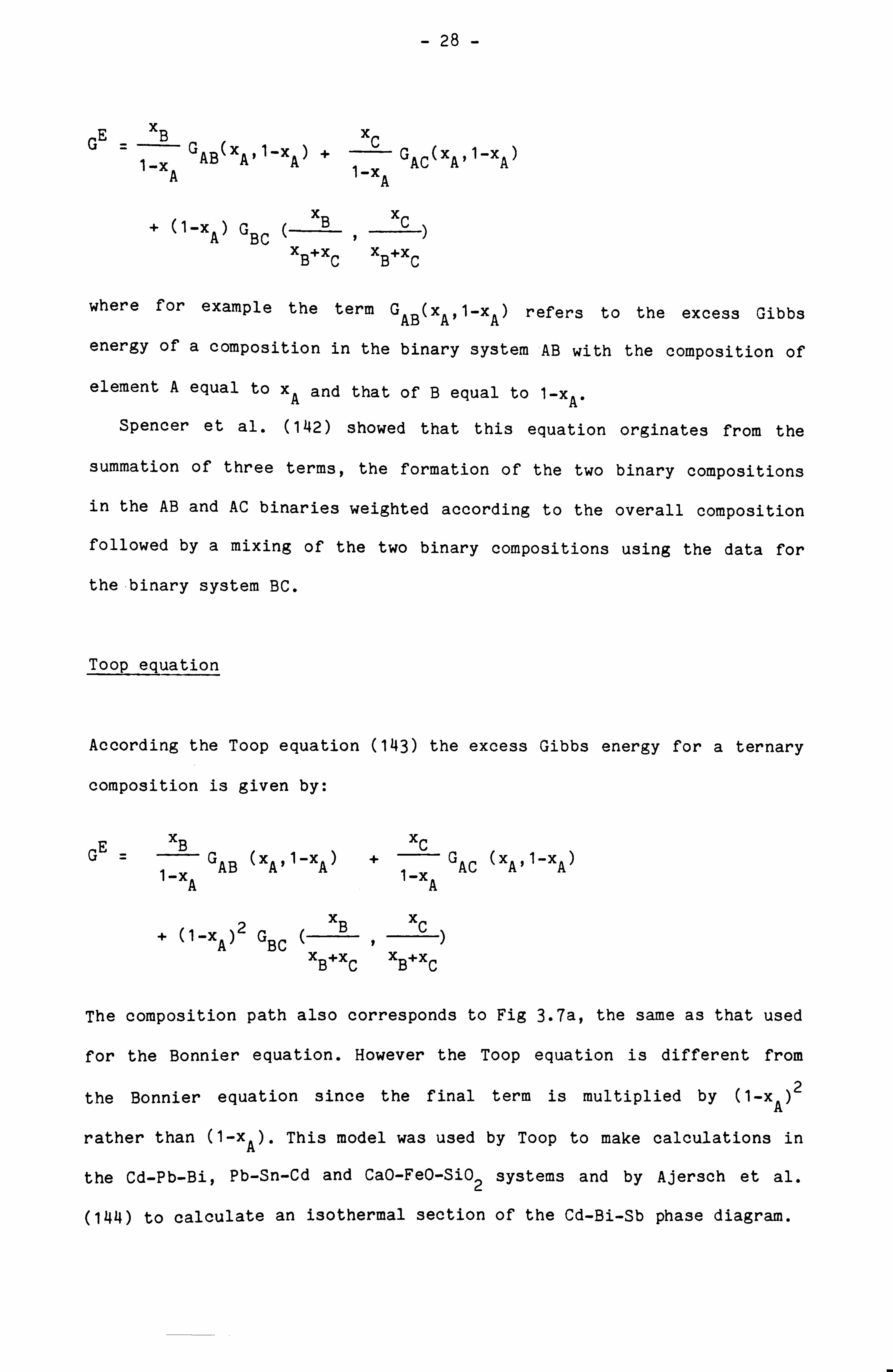
Toop equation
According the Toop equation (143) the excess Gibbs energy for a ternary
composition is given by:
XX
GE = GAB (xA, 1-xA) +C GAC (xA, 1-xA) 1-xA 1-xA
+ (1-xA)2 G BC (
xB
,
xC )
xB+xC xB+xC
The composition path also corresponds to Fig 3.7a, the same as that used
for the Bonnier equation. However the Toop equation is different from
the Bonnier equation since the final term is multiplied by (1-xA)2
rather than (1-xA). This model was used by Toop to make calculations in
the Cd-Pb-Bi, Pb-Sn-Cd and CaO-FeO-Si02 systems and by Ajersch et al.
(144) to calculate an isothermal section of the Cd-Bi-Sb phase diagram.
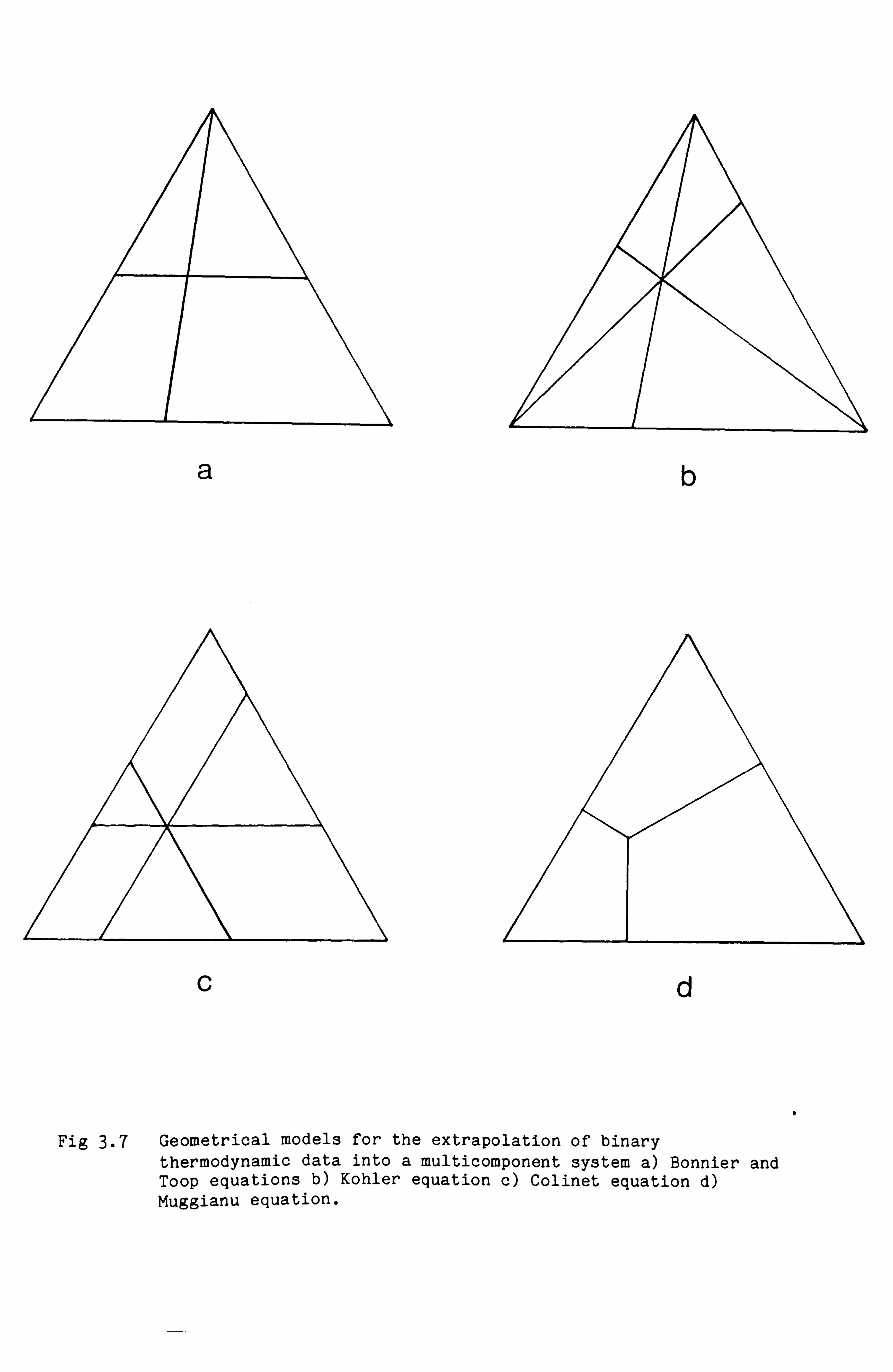
a
C
b
d
Fig 3.7 Geometrical models for the extrapolation of binary thermodynamic data into a multicomponent system a) Bonnier and Toop equations b) Kohler equation c) Colinet equation d) Muggianu equation.
10

- 29 -
Kohler equation
Kohler (145) and Olson and Toop (146) derived the following equation
independently.
(AXB GE (xA + xB)2 GAB X
xA+xB xA+xB
xx + (xA + xc)2 GAC (A)
xA+Xc xA+Xc
+ (xB + xc)2 G BC (
xB xC 9
XB+XC XB+XC
which is shown as the composition path in Fig 3.7b. The Kohler equation
has been extended into a generalised multicomponent system by Kehiaian
(147) and has been used extensively by Kaufman (148-159) and others
(160,161).
Both the Kohler equation and the Toop equation have their base in a
completely rigorous treatment of Darken (162) in which he showed that
for a ternary system A-B-C the excess free energy may be calculated from
true binary terms for the A-B and A-C systems and a term for a pseudo
binary section along a line of constant B/C ratio.
Colinet equation
For the Colinet equation (163) the excess Gibbs energy is given by:
Xx
GE = 1/2 [A GAB (1-xB, xB) +B GAB (xA, 1-xA) 1-xB 1-xA
+ XA
G (1_x ,x)+
xC G (x , 1_x )
1_x AC CC l_x AC AA CA
)] + xB
G BC (1-x
C, xC )+ xC
G BC (x
B' 1-x B
1-x 1-x cB

- 30 -
as shown in the composition path Fig 3.7c. The Colinet equation is
rarely used.
Muggianu equation
The composition path used by the Muggianu equation (164) was called by
Jacobs and Fitzner (165) 'the shortest composition path' as in Fig 3.7d.
The excess Gibbs energy is given by:
GE 4xAxB
(2xA+xc)(2xB+xC)
4xAxC
(2xA+xB)(2xc+xB)
IxBxC
(2xB+xA)(2xc+XA)
GAB (xA+xc/2, xB+xC/2)
GAS (xA+xB/2, xc+xB/2)
G BC (xB+xA/2, xC+xA/2)
This expression may seem complex but, as shown by Jacobs and Fitzner and
Hillert (166), if the binary systems are represented by the
Redlich-Kister expression the expression simplifies to
GE =xAxB (LAB + LAB(xA-xB) + LÄB(xA-xB)2 ..... )
+ xAxC (LÄC + LÄC (xA-xc) + LÄC (xA-xc)2 .... )
+ xBxC (LBC + LBC (XB-xC) + LBC (xB-xC)2 .... )
This is simply the ternary Redlich-Kister expression (139) and has been
used at NPL for many years (167-169).

- 31 -
h) Comparison between geometrical equations
These equations have been compared in a number of papers
(79,80,142,143,165,166,170,171). From the theoretical point of view none
of the models can be considered to be anything other than an
approximation. Nevertheless the models can be tested for certain
desirable features such as compatibility with the regular solution
model, symmetric behaviour with respect to the pure components and
correct limiting behaviour when the amount of one of the components
becomes zero or when two elements have very similar properties.
Of the five models both the Bonnier and the Toop models are
unsymmetrical with respect to the pure components. The Bonnier model is
little used now since it is not consistent with the regular solution
model. The Toop model is used for systems only where one component is
very different from the others. The other three models are all
symmetrical and consistent with the regular solution model.
Unfortunately none of them transform to a binary data set when two of
the elements become very similar. Hillert (166) compared the Kohler,
Colinet and Muggianu models in detail by deriving expressions for the
ternary excess Gibbs energy representing the three component binary
systems by the subregular model. He showed that, despite the different
composition paths, the Colinet and Muggianu methods give identical
results. Furthermore the difference between these models and the Kohler
model will always be very small.
In the other papers the predictions of the models were compared with
available experimental information. They found essentially that all
these models represent the data reasonably well and that there is no
overriding reason why one model should be chosen in preference to
another. The model used at NPL and in this thesis for metallic systems
is the full ternary Redlich-Kister expression with a ternary interaction

- 32 -
term given by:
nn Aft x1Gi + RT 7 xi in xi
i=1 i=1
n-1 n + xixj (Lýj + L1 (xi - xj) + L2 (xi - xj)2 ..... )
n-2 n-1 n +2Z
i=1 j=i+1 k=j+1 xixýxk Kijk
i) Models for solid 'compound' phases
In many systems of practical interest the interatomic forces have
sufficient strength to favour phases for certain ranges of composition
where different types of atom occupy preferentially different types of
lattice site. Such phases are often loosely described as compounds.
These 'compound' phases often coexist within the same system as the
so-called substitutional phases discussed earlier. Often within a binary
system these compound phases have a very narrow range of homogeneity and
it is common to treat such phases as having a fixed stoichiometry.
In a ternary system it is common for a third element, say C, again to
enter into one particular type of site eg. the type occupied by B in the
compound ApBQ and to substitute for element B. If the compound ApCQ were
stable in this particular structure we might have a line representing
the phase from ApBq to ApCq in the phase diagram as in Fig 3.8. These
so-called 'line-compounds' are very common in systems of practical
interest. Of ten the compound ApCQ with this structure is not actually
stable in the A-C binary system, but it is still convenient to think of
the hypothetical form, obviously with a higher Gibbs energy than the
stable phase assemblage for that composition.
The thermodynamic data for such a 'line-compound' phase are naturally
related back to the data for the pure compounds. A number of equivalent

A
B
Fig 3.8 Ternary 'line-compound' phase between binary stoichiometric
C
compounds ApBq and ApCQ.

- 33 -
approaches have been adopted (46,172-174) based on the assumption of
ideal mixing between the atoms on the same type of site or sublattice
with a superimposed interaction expressed in a way analogous to the
regular solution model or power series expansion.
This gives an expression of the form:
-XX ýf'G B
fGA B+S AG
fAC qP4qPQ
+RT[ xB ln(xB)
+ xB xC L
+ xc ln(xc) - (1-xA) ln(1-xA) 3
where the Gibbs energy of formation of the line-compound refers to one
mole of material while the Gibbs energies of the binary stoichiometric
compounds refer to one mole of formula unit.
This approach was generalised by Sundman and Agren (175),
incorporating work of Hillert and Staffansson (176) and Harvig (177),
into a form suitable for computer application for phases with any number
of components and sublattices. A key feature of their approach is the
use of site fractions ie. the fraction of one sublattice occupied by one
particular type of atom.
Some classes of phases exhibit appreciable ranges of homogeneity
within binary systems and it is no longer always possible to treat these
phases as stoichiometric. The effect of non-stoichiometry on the
thermodynamic properties was first studied in detail by Wagner and
Schottky (178) and their work has been extended by Libowitz (179,180)
and Brebrick (181). Any deviations from stoichiometry are due to some
imperfections in the lattice. By assigning energies to each of the
possible point defects it is possible to account for the variation of
the Gibbs energy with composition.
-34º-
The systematic sublattice approach of Sundman and Agren (175) has
also been used to describe the thermodynamic data for these
non-stoichiometric compounds. Here however the data are not energies for
each point defect but interactions between atoms or vacancies within the
same sublattice together with data for hypothetical pure compounds. This
approach has been used with success for the sigma phase (182,183)
j) Molten Salt Solutions
One area of particular interest for modelling thermodynamic data is
in molten halide solutions. As with alloy systems the simplest model,
the so-called Temkin model (184), is one for ideal mixing although here
the mixing of cations and anions is assumed to take place independently.
Nearest neighbour interactions have been allowed for in the model of
Flood et al. (185) and in Forland's extension (186).
The similarity between these models and those used for alloy systems
has led various groups to apply power series expressions such as the
Redlich-Kister model to these molten salts. For example Chart (187) has
derived data for the component binary systems of the KC1-CaC12-ZnC12
system and calculated ternary phase equilibria which are in excellent
agreement with experimental measurements. Similarly Oonk et al.
(188-190) have derived data for a wide range of alkali halide binary
systems.
A completely new model has been introduced by Saboungi and Blander
(191-193) called the Conformal Ionic Solution (CIS) theory which they
describe as a statistical mechanical perturbation theory. The model has
been used by Pelton et al. (194,195) for a number of molten salt systems
including carbonates, hydroxides and sulphates.
A problem arises where the mixing occurs between ions of different
charge eg. in the KC1-CaC12 system. In the work discussed so far

_35_
components were chosen such that one mole of solution contains one mole
of the ions that are mixing and this is identical to the approach
recommended by Hillert et al. in their generalised lattice model of the
liquid phase (196).
Molten oxide systems are particularly important types of molten salt
system. Kaufman (152,155) has chosen a different model from those
described above derived from a substitutional model with oxygen as a
component but where the composition has been constrained to lie between
binary stoichiometric oxides. These oxides were expressed in terms of a
mole of atoms rather than moles of metal ions and he derived data for a
wide range of systems between Cr203, MgO, A1203, Fe203, Fe304, FeO,
Si02, and CaO using a temperature dependent two coefficient expression.
For some of these pseudo binary systems e. g. CaO-Si02, he found that it
was necessary to split the systems into two ranges of composition.
Howald et al. (197-201) have also derived data for some oxide
systems. The data were represented by Redlich-Kister polynomials in
terms of the proportions of the metal ions e. g. proportions of the
Na00.5 in the system Na00.5-Si02. They also found that the CaO-Si02
system was too complex to f it with one expression. The CaO-Si02 system
has also been represented with power series expressions by Kaestle and
Koch (202) and Lumsden (203).
The problems found in representing the data for some of these oxide
systems implies the need for a closer examination of the structure of
these phases. Attempts to do this will be described later.
k) Metal-Salt Systems
The liquid phase for metal-salt systems eg. in sulphide systems is
especially difficult to model thermodynamically. Attempts have been made
to represent the data with power series or equivalent expressions (161)

- 36 -
but the large number of coefficients required makes this approach of
little use.
The two most useful approaches to understanding the data for these
systems have been the associated species model (204-228) and a
sublattice model with vacancies (229-235). Measured data for these
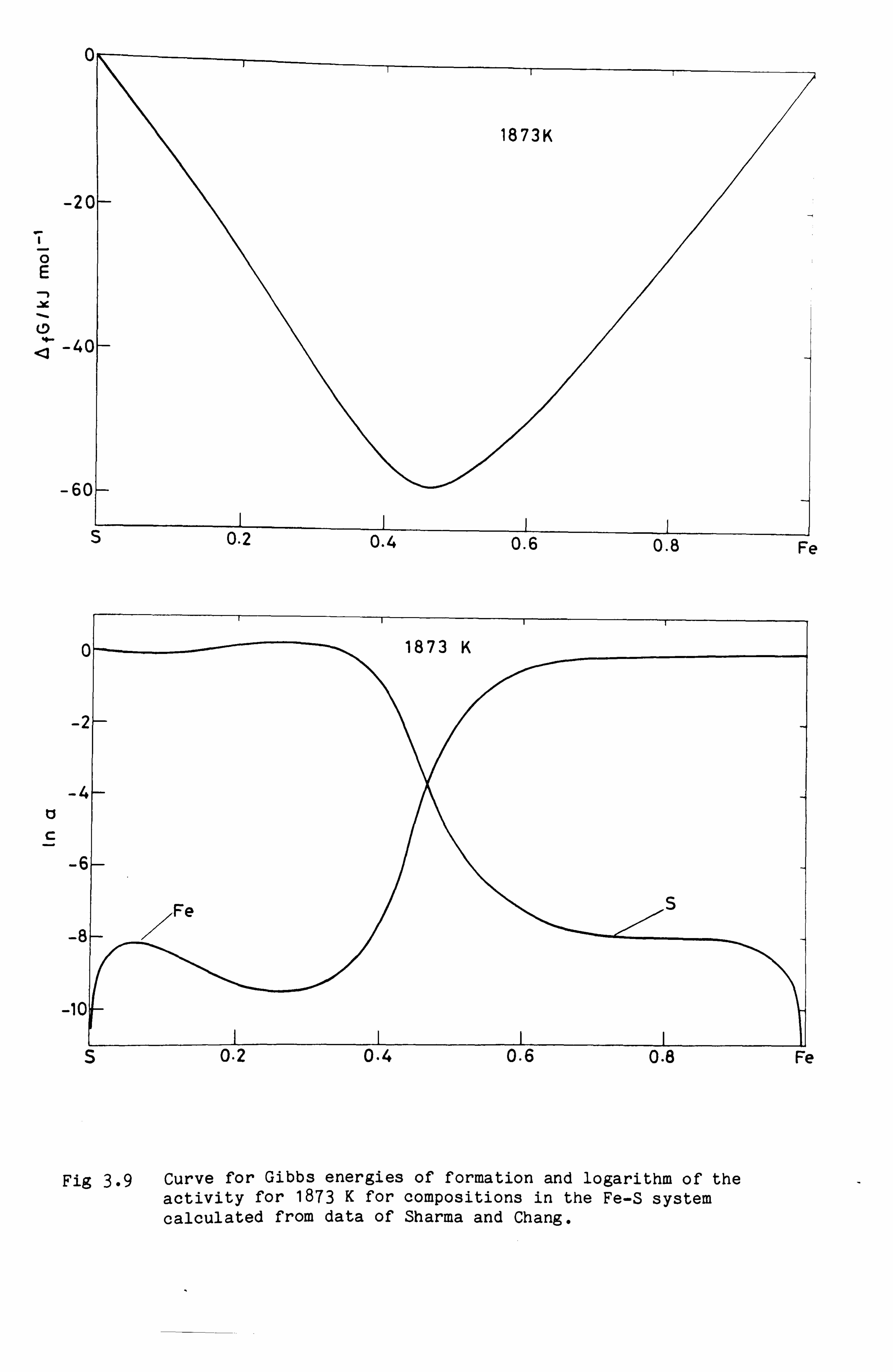
liquid phases are often characterised by an abrupt change in the
activity of one of the components and a sharp minimum in the Gibbs
energy function such as is shown in Fig. 3.9. The compositions of these
abrupt changes often seem to correspond to the composition of a solid
phase which itself exhibits a range of homogeneity.
The associated solution model, has been much used over the last few
years. It postulates that the phase consists of distinct molecular
aggregates rather like the gas phase which shows similar dramatic
changes in thermodynamic properties at certain compositions. In the case
of the liquid phase the various species would interact with one another.
As an example, Sharma and Chang (204) for the Cu-S system proposed
the existence of Cu2S species in addition to the elemental species of
copper and sulphur. Species of Cu2S were chosen because the
thermodynamic properties of the liquid phase changed abruptly at about
this composition. For an overall composition xCu and xS the model
postulates that some of the copper and sulphur atoms combine to form
species of Cu2S. If the fractions of the species are YCu 2 S' yS and YCu'
it can be shown that:
YCu = xCu -2 YCu2S xs and YS = xs - yCu2s (1-2xs)
For this overall composition the relative amounts of the various
species are not defined directly but depend upon the affinity of the
elements for forming the associated species. These relative amounts must
be calculated by some iterative procedure in order to find the
0
-20
0 E Y
-40
-60
S
C
-2
-4
c
-6
-8
-10
1873 K
Fe
S 0.2 0.4 0.6 0.8 Fe
Fig 3.9 Curve for Gibbs energies of formation and logarithm of the activity for 1873 K for compositions in the Fe-S system calculated from data of Sharma and Chang.
U. ' 0.4 0.6 0.8 Fe

- 37 -
conditions which give the minimum Gibbs energy of formation. This can be
calculated as the sum of terms for the formation of the associated
species and the normal expression for a ternary system with random
mixing and interactions between the species, the latter being expressed
by a Redlich-Kister power series.
The concept of postulating associate species in condensed solution
phases was introduced and developed a number of years ago (205-208) but
it was Jordan (209-211) who first used this for metallic systems. The
model, which has been reviewed by Gerling et al. (212) has been very
successful for representing the thermodynamic data for the liquid phase
in a number of systems (204-227). It has also been used to represent the
thermodynamic data for solid phases (218,228) including those
traditionally represented by a substitutional model.
The application of a sublattice model to high affinity liquids was
suggested by Hillert et al. (176,196,229-233) and Brebrick (234) and
extended in this present work (see chapter 8 and ref. 235). Here the
approach is directly analogous to the models used for condensed compound
phases which exhibit wide ranges of homogeneity and abrupt changes in
the thermodynamic properties similar to those observed for the liquid
phase. The use of this model implies that for these systems some aspects
of the solid lattice structure are retained on fusion.
The sublattice model was first tested by Hillert and Staffansson for
the liquid phase in the metal rich portion of the Fe-S (229) and Mn-S
(230) systems and to calculate the metal rich part of the Fe-Mn-S system
(231). Here they assumed that the liquid phase consisted of two
sublattices with an equal number of sites. The first sublattice was
completely filled with metal atoms while the second sublattice consisted
of sulphur atoms and vacancies.
Recently the model was extended by Fernandez Guillermet et al.
(232,233) to represent the liquid phase for the whole of the Fe-S
- 38 -
system. For this, vacancies were introduced into the metal sublattice in
addition to the sulphur sublattice. The Gibbs energy for a composition
in the phase is expressed as the sum of three terms - the first for the
Gibbs energies of formation of pure compounds formed by filling each of
the sublattices with its constituents. Hence there are four compounds
FeVa, FeS, VaS and VaVa,. The second term is in two parts to represent
the ideal mixing of the constituents in each of the two sublattices. The
third term represents the interactions between the different
constituents on the sublattices. The details of this expression will be
shown in a chapter 8. Also it will be demonstrated how this approach has
been used and extended to extrapolate data into the Fe-Cu-Ni-S liquid
phase. For a given composition the vacancy concentration is not defined
and a process of iteration must be used to find the condition which
gives the lowest Gibbs energy.
Recently Hillert et al. (196) have suggested a new model for
representing the data for the liquid phase. For the Fe-S system for
example there would no longer be the same number of sites in the two
sublattices. Instead the ratio of the number of sites would be
determined by a condition of electroneutrality between the ionic
constituents of the sublattices. In addition the new model excludes
vacancies from the metal sublattice which now consists simply of Fe2+
ions but introduces sulphur atoms on the sulphur sublattice in addition
to S2 and negatively charged vacancies.
This new model has two particularly interesting features. Firstly it
was shown that as the system develops lower affinity the expression for
the Gibbs energy approaches that for a substitutional solution. Secondly
for a binary system the expression for the Gibbs energy is identical to
that derived for an associated solution provided that the associate
species contain one atom only of the electronegative element.

- 39 -
1) Silicate Systems
It was pointed out earlier that for certain oxide systems, in
particular silicates, the power series approach derived for an
essentially substitutional solution is not well suited to representing
the thermodynamic data adequately. For these complex systems certainly,
the use of an incorrect model cannot allow us to extrapolate binary data
into multicomponent systems with any confidence. The success of the
associated solution model and the multiple sublattice model in
representing data for sulphides and other systems has implied that they
could be used for molten silicate systems. As yet the multiple
sublattice model has not been tested. Attempts to use the new model for
the liquid phase derived by Hillert et al. (196) would be of great
interest.
The associated solution model has been used with some success by
Bottinga and Richet (236) and by Goel et al. (228) for the Fe-0-SiO 2
system. Goel et al. introduced species of Fe, FeO, FeO 1.5 and Si02 and
the data for these species and the interaction between them gave
remarkably good agreement over the whole system. However a large number
of parameters is required for this model and it should not be thought of
as an assessment but rather as a very good correlation of the observed
properties.
Many other models have been developed to represent the thermodynamic
data through a close examination of the structure of silicates. In these
models it is a generally accepted principle that every silicon atom is
tetrahedrally surrounded by oxygen atoms. Two basic mechanisms can be
considered as limiting cases. In very basic slags ie. slags with low
silica content, the structure can be thought of in terms of M2+, 02 and
SiO (orthosilicate) ions. This is the approach introduced by Flood and

-40-
Knapp (237) and the thermodynamic data can be thought of in terms of the
formation of the orthosilicate ion and the random distribution of the
02 and SiO4- anions. The addition of more silica leads to the formation
of more complex silicates. At the silica rich side of the system ie. for
acidic slags one could expect the mechanism of Fincham and Richardson
(238) to operate whereby one oxide anion breaks down a bridge formed by
another oxygen atom joined to two silicon atoms.
In a number of these silicate systems there is immiscibility between
basic and acidic slags e. g. in the FeO-Si02 and CaO-Si02 systems where
the metal oxide typically dissolves in the silica up to about 5%. In
general there is always considerably higher solubility of silica in the
metal oxide. In some systems, e. g. A1203-Si02 there is complete
miscibility between basic and acidic slags where it is believed the
aluminium atom can substitute directly for silicon atoms.
Flood and Knapp (237) extended the description of very basic slags
which consists of M2+, 02 and SiO14 ions by including other polymeric
anions. From a study of the PbO-Si02 system they concluded that the
addition of Si3O 6- and Si606- anions mixing ideally resulted in a good 9 15
representation of the thermodynamic data for compositions up to 60 mole
% Si02, This approach was adopted recently by Bjorkman et al. (239,240)
for the PbO-Si02 and Fe-0-SiO 2 systems using more complexes than
suggested by Flood and Knapp. The description of Bjorkman et al. is
limited to basic slags.
Other models for liquid silicates have been reviewed by Gaskell (241)
and Bottinga et al. (242) which take their basis from the work of Toop
and Samis (243). This is in itself an extension of the work of Fincham
and Richardson (238) mentioned earlier. The breakdown of an oxygen
bridge by an oxide ion can be written in terms of:
200+ 02-

- 41 -
where 00,0- and 02- represent bridging oxygen atoms, singly bonded
oxygen atoms and free oxide ions. According to Toop and Samis an
equilibrium constant can be written for this reaction:
k= LOO I [02 -1
Co-]2
where k is a constant for a given temperature and a given metal ion ie.
independent of composition of the melt and the complex ions involved.
The Gibbs energy of formation from pure liquid components would be
written by:
, QfG =1 [0-] RT ln(k)
2
which implies ideal mixing between the three types of oxygen atom. This
simple model gave good quantitative agreement with experimental
information and led Toop and Samis to perform calculations in the
CaO-FeO-Si02 system at 1600°C.
This approach was extended by Masson (244-246) who applied polymer
theory to the breakdown of the silicon-oxygen-silicon chains. Kapoor
(247-249) developed the polymerisation approach using statistical
thermodynamics and used an approach of Guggenheim (93) for the
configurational entropy of mixing rather than the Temkin expression.
A completely new approach was adopted by Yokokawa and Niwa (250) who
considered a silicate melt in terms of a basic sublattice of oxygen
atoms or ions with silicon atoms occupying a proportion of the
tetrahedrally coordinated sites, the rest remaining vacant. This model
was adopted by Borgianni and Granati (251,252) for use in Monte Carlo
calculations.
A more empirical approach was adopted by Lin and Pelton (253) who
also considered the melt as a lattice. According to this treatment
oolyrneric anions are not considered directly since the configurational

- 42 -
entropy is calculated simply from the distribution of the different
types of 'structural units' (silica tetrahedra, 02 ions and oxygen
bridges) throughout the melt. Furthermore the enthalpy change for the
breakage of oxygen bridges was considered to be independent of the
composition of the melt. The results they obtained were in excellent
agreement with those determined eyperimentally. This model has two great
strengths. Firstly the polymeric ions, although not treated explicitly,
can be examined for each calculation through analysis of the
probabilities of various ionic configurations. Secondly unlike all the
other structural models discussed, the approach of Lin and Pelton is
applicable to the whole composition range from basic to acidic slags.
More recently Blander and Pelton (254) have devised a new empirical
model for slags as an attempt to devise a method for analysing data for
multicomponent systems. The model, an 'ad-hoc modification of the
quasi-chemical theory' appears to have been very successful.
Summ
A number of different approaches have been used to model
thermodynamic data for metallurgical systems. Some of these have been
described in this chapter. This area of work is assuming greater
industrial importance and can be expected to develop significantly over
the next few years as industry becomes more demanding in its needs for
data.
- 43 -
CHAPTER 4
The Role of the Computer in Thermodynamics
Introduction
The principles involved in the use of thermodynamics for the
calculation of phase equilibria and many of the models which can be used
to represent thermodynamic data for various phases are now well
established. However the calculations themselves, except for the
simplest cases are quite complex and generally require the use of a
computer in order to search for the compositions and amounts of the
competing phases which give the lowest Gibbs energy. Many different
types of computer program have been developed for the calculation of
phase equilibria as will be described below. Computers are now also
becoming essential for the reverse process when, during the critical
assessment of thermodynamic data, parameters for the thermodynamic
models are derived from known equilibrium properties. Large data files
are often required for both the critical assessment of data and the
calculation of complex equilibria and this has led to a third use for
computers ie. that in the storage of data in computer based databanks
which ultimately leads to greater reliability and efficiency.
Calculation of Equilibria
One of the first computer databanks developed for the storage of
thermodynamic data was the NPL MTDATA system (255-258) which has been
offered on-line within the UK for a number of years over the telephone
or a packet switching network, and now forms part of the CSIRO system
within Australia (259). Until 1980 it also formed part of the MANLABS
system within the USA (260). It contains data for pure condensed
- 44 -
substances, gaseous species and dilute solutions, and in the on-line
service is used to tabulate, for various temperatures, the thermodynamic
properties of pure substances or the change in these properties during a
chemical reaction. Originally the databank was designed for a mainframe
computer but it has now been modified at NPL for implementation on
microcomputers (261).
Since then similar databanks have been developed elsewhere. In
Canada, Pelton, Bale and Thompson (262,263) in Montreal have constructed
the FACT databank service, which is available on-line throughout North
America, and offers rather more extensive facilities than that developed
by Alcock and Goetze (264) in Toronto. In Moscow the IVTAN group have
been augmenting their data compilations with a computerised databank
while within Western Europe, equivalent databanks have also been
developed in Uppsala (265), Grenoble (266), Aachen (267-269) and
Harwell. These last three groups are now working with NPL and others
within Europe to construct a joint database and on-line databank system
through the organisation SGTE.
Although tables or plots of the change in thermodynamic properties
for chemical reactions are useful in predicting simple types of
equilibria more sophisticated software must be used for complex
equilibria. One such type of calculation for multicomponent equilibria
between gaseous and condensed phases is to produce a so-called
Predominance Area or Pourbaix diagram such as is shown in Fig 4.1 where
the partial pressure of one of the gaseous species is plotted against
the temperature or the partial pressure of another species. A number of
programs have been developed to calculated these diagrams, many of them
linked to databank systems eg. those of Barry (270,271), Pelton and Bale
(262) and Barin et al. (267,268).
More sophisticated still are the programs used to calculate
equilibria, for a given overall composition, between various gaseous

2
0
_2
G
cý v
0 to a cm - 0
-10
-12
-14
Fe S04
Fe2 (S04 )3
FeS2
Fe203 Fe S Fe 304
Wustite Fe
-30 -25 -20 - -15 -10 -5 0 log p 02 (G)/atm
Fig 4.1 Predominance Area diagram for the Fe-S-O system calculated by Barry showing regions of stability for the various condensed phases as a function of the partial pressures of SO2 and 0 2.

-u5-
species and condensed phases. This problem is often known as Gibbs
energy minimisation although the mathematical formalism can be expressed
in other equivalent ways. The search for reliable and efficient programs
has attracted many groups of scientists and mathematicians and many of
these programs have been reviewed by Smith (272,273) and van Zeggeren
and Storey (274).
Perhaps the most widely used program and certainly one of the most
versatile is Eriksson's SOLGASMIX. This program was originally designed
for equilibria between a gaseous phase and condensed stoichiometric
phases (275,276) but it has been extended to include condensed solution
phases (277). It has also now been linked to many substance databanks
eg. by Gallagher (269), Turnbull (278), Thompson (279) and by Dinsdale
to allow these calculations to be performed quickly and in a routine
fashion. SOLGASMIX has also been adapted for speciation calculations
within dilute aqueous solutions and their equilibria with a gas and
stoichiometric solid phases. In this program, SOLGASWATER (280), water
is assumed to be at unit activity. The versatility of SOLGASMIX is
perhaps best shown in its use in the program SOLGASMIX-REACTOR (281)
when predicting, in detail, the behaviour of an industrial process.
SOLGASMIX-REACTOR in many respects reflects the ultimate aim for these
types of calculation. By breaking down a complex industrial process into
a number of levels and linking the thermodynamic data to details of the
process SOLGASMIX-REACTOR can be used to predict conditions to obtain
the maximum yield or the minimum consumption of energy.
Another example of where these types of calculations can be linked
directly to an industrial process is in the prediction of the optimum
conditions for Chemical Vapour Deposition and the growth of crystals.
One such program for these calculations has been developed by Nolang and
Richardson (282-287) in Uppsala consisting of a database with packages
for the calculation of predominance area diagrams, transport flux and

- 46 -
chemical equilibria. It has been used, for example, to improve growth of
crystals of yttrium iron garnet. Similar calculations have been
performed by Bernard et al. (17).
At the same time as programs were being developed to calculate the
equilibria between gas phase species and stoichiometric compound phases,
interest was also being focussed on routines and programs for the
calculation of multicomponent phase diagrams for condensed solution
phases especially alloys. Much of the early work in this field was done
by Kaufman and his colleagues (46) who developed computer programs and
also many of the datasets commonly used.
Other early work has been carried out by Ansara et al. (79,288) and
Counsell et al. (289). The work of Counsell et al. was extended by
Dinsdale (15,173) who developed an on-line databank system, ALLOYDATA,
containing critically assessed binary and ternary thermodynamic data
linked to software for the calculation of multicomponent phase diagrams.
Lukas (290) has also made significant contributions towards routines for
the calculation of phase equilibria.
More recently great advances have been made at the Royal Institute of
Technology in Stockholm under the direction of Hillert. Sundman (291)
has developed a sophisticated subroutine package, Gibbs Energy System,
for calculating the Gibbs energy and its derivatives for a very general
representation of thermodynamic data involving multiple sublattices.
This subroutine package is used in particular by the program POLY
developed by Jansson (292) for the calculation of binary and
multicomponent phase equilibria for alloys. POLY is undoubtedly the most
sophisticated program of its type available at present. Both the Gibbs
Energy System and POLY are in turn used as subroutine packages to a
third program developed by Agren (293-295) for the prediction of phase
transformations and diffusion related equilibria.
The division between the two types of programs, one designed to

- 47 -
calculate essentially the distribution of species within the gas phase
or aqueous solution and the other to calculate the equilibrium between
different condensed solution phases is somewhat arbitrary although the
two problems make different demands in terms of the numerical analysis
routines. Furthermore under certain circumstances it is important to
solve both kinds of problem simultaneously e. g. corrosion of superalloys
by gaseous environments, and consequently programs have now been written
to perform these more complex calculations. Of particular note is the
program of Eriksson, SOLGASMIX, which has recently been used for
calculations of multicomponent alloy phase diagrams (296). Eriksson
himself has recently reported most ambitious calculations, carried out
using SOLGASMIX in conjunction with Saxena, of equilibrium mineral
assemblages on cooling down a gas of solar composition (297,298). The
aim was to further understanding of the formation of planets and
meteorites. Here the phases involved included a gas phase, liquid and
solid alloy phases, various solid oxide phases of variable composition,
a carbide solution phase and various stoichiometric phases such as
sulphides, nitrides and hydrides. They included 14 elements in their
calculations. SOLGASMIX has been used here to calculate equilibria in a
nine component alloy system as will be shown in chapter 7.
Jansson (299,300) has now developed a new and extremely general
program POLY-II based upon the ideas of Hillert (301,302) and linked to
the Gibbs Energy System. This program has been designed to include
speciation calculations for the gas phase in addition to the
multicomponent phase equilibrium calculations involving alloys. Present
tests seem to indicate that performance for speciation calculations is
inferior to that of SOLGASMIX. More recently Hodson (303) at NPL has
developed a program MULTIPHASE to allow simultaneous calculations
involving the gas phase, aqueous phase and various condensed non ideal
solution phases. The program is extremely reliable and efficient.
- 48 -
To date none of these sophisticated types of programs have been
linked to an extensive database comprising, for example, data for
alloys, aqueous solutions, gases and other phases of importance. This is
one of the major aims of the organisation SGTE and it is planned to have
such a databank available on-line throughout the world by early 1986.
Although it is recognised that the major users of such a service would
be the member organisations of SGTE the databank is being designed to
encourage industries and universities to use extensively. To this end,
SGTE has made major efforts to design the outer appearance of the
databank so that the user finds it easy and convenient to use and can
find his way through the system with a minimum of tuition.
Critical Assessment of Data
The computer is also rapidly becoming completely indispensible for
the critical assessment of thermodynamic data. For pure substances, the
computer has been used mainly for the calculation of the thermodynamic
properties of gas phase species from statistical mechanics and
subsequently fitting the heat capacity data to a convenient power series
expression. More recently, work has begun, pioneered by Pedley et al.
(304) to optimise enthalpies of formation from measurements of the
thermodynamic data (e. g. partial pressures, equilibrium constants,
formation measurements) for the various reaction networks that relate
substances to one another. As an example a consistent set of the
enthalpies of formation at 298.15 K and thermal functions (energy and
heat capacity data) of gaseous metal oxides have been obtained.
Ambitious plans are now under consideration to incorporate all such
experimental data for pure substances into a computer database. By
linking this database to Pedley's program any new experimental
measurements can immediately result in a revised set of thermodynamic

- 49 -
data.
For condensed solution phases eg. in alloy systems, the role of the
computer in the critical assessment of data is even more important than
for pure substances. Firstly the data for condensed solution phases are
normally more complicated than data for gases requiring the use of a
variety of different models for representation as shown in the last
chapter. The computer is ideal for repetitive calculations of the
thermodynamic properties for these phases. Secondly the types of
experimental data are more diverse including many types of measurements
of thermodynamic properties and phase equilibria in addition to
intuitive information that the assessor may need to provide. The
computer would normally be used to calculate the agreement between the
measured values and those calculated from a set of parameters often
involving quite complex calculations of equilibria. The computer can
then minimise these errors and find automatically the best set of
parameters.
Normally this type of program is used for the assessment of data for
binary systems. However it is important to realise that data are
required for phases not just in the regions where they are stable but
generally across the whole of the system as shown in the last chapter.
An optimisation type of assessment program is ideal for this where, for
example, the experimental extension of a phase, stable in only one
binary system, into a ternary system can be used to derive data for this
phase for the other two binary systems.
The assessment of thermodynamic data direct from phase diagram
information was first suggested by Hiskes and Tiller (305-307), Rao et
al. (308) and Chiotti et al. (309). Since then others, in particular
Lukas et al. (310-312) , Boyle et al. (313) , Jansson (314,315) , Sundman
(316), Pelton and Bale (317) and Oonk et al. (188,318-321) have
developed computer procedures to carry out such calculations. The work

- 50 -
of Lukas is particularly important since the programs are very portable,
widely used and allow choice of a number of models to represent the
data. Versions of the program are now available for binary, ternary and
quaternary systems.
It is also worth noting the program of Jansson, PARROT (314,315),
which is connected to the suite of programs referred to earlier
including POLY, Gibbs Energy System and POLY-II. These provide a highly
flexible framework for all assessment work.
Conclusions
The role of the computer in thermodynamics is now so well established
that it is difficult to contemplate a time when computers were not
available. In the future this role can only increase as large databases
are constructed containing not just critically assessed data but also
the raw experimental data. The computer also has enormous potential as a
teaching aid. If all the tiresome and errorprone arithmetic were
collected within a reliable computer program, a student would be able to
concentrate on the basic principles of the subject and their application
to industrial processes. It has even been suggested (302) that in the
future little thermodynamics as such need be taught other than the
general principles and how databanks could be interrogated to solve
particular equilibrium calculations. Certainly we can look forward to
the most complicated equilibrium calculations being carried out with
great reliability and ease. Furthermore the work of Agren (293-295),
Eriksson (281) and Nolang and Richardson (283-287) points the way to the
use of the computer and thermodynamic data for modelling problems
occurring in practical chemical and metallurgical industry. Certainly
the incorporation of databank packages in expert systems (322) will be
of utmost importance.
- 51 -
CHAPTER 5
Development of Computational Procedures for the
Calculation of Binary Phase Diagrams
Introduction
Over the last few years the computer aided calculation of phase
diagrams from thermodynamic data has become widely accepted as a most
useful tool to assist in the solution of industrial problems. This has
led to the search for reliable and efficient procedures to facilitate
these calculations. Many of the programs developed so far have been
designed for use on main-frame computers. With the advent of desk top
or even hand held microcomputers it is also important to develop
compact programs.
Discussed in this chapter is the mathematical basis for a program
used to calculate binary phase diagrams automatically. It is hoped
that these techniques will be of benefit in the critical assessment of
thermodynamic data and also highlight some major problems to be
overcome for the automatic calculation of multicomponent phase
diagrams. In particular a very compact and reliable method has been
developed to calculate efficiently binary phase equilibria for a fixed
temperature. It is shown how this method can be extended to predict
the changes in the phase boundaries with variation of temperature.
Finally a generalised procedure is described which can be used to
calculate all the stable phase boundaries in a binary system for a
given temperature. Through use of this procedure binary phase diagrams
can be calculated automatically.
Often in the past direct calculation of phase equilibria in binary
- 52 -
systems was avoided and instead the Gibbs energies of formation for
the different phases involved in the alloy system were plotted out and
the phase boundaries determined manually by using the well known
common tangent construction (45) shown in Fig 5.1. The phase diagram
could be built up by following this procedure for a number of
temperatures. In order for a computer to calculate phase diagrams
automatically, it would need to search for conditions either giving
these common tangents or the minimum Gibbs energy of formation of a
composition within the two phase region. Of course, these two methods
are equivalent as will be shown later.
A number of methods for calculating equilibria in binary alloy
systems have been reported. The basic principles have been described
by Ansara (79), Hillert (323,324), Oonk (318,325) and Kaufman and
Bernstein (46). Hillert (324) also suggested use of a particular
method based upon the partition function and the partial molar Gibbs
energies. Gale and Davis (326) used a steepest descent algorithm to
solve a pair of non-linear equations and calculate the composition of
the alloy phases in equilibrium. Kaufman and Bernstein (46), Gaye and
Lupis (327,328), Tomiska et al. (329) and Henig et al. (330) have
solved similar equations based on the partial molar Gibbs energies by
using the Newton-Raphson procedure (page 56). Gaye and Lupis moreover
developed their technique to facilitate calculations over a range of
temperatures. Pelton et al. (331) have developed a stepwise iteration
procedure to calculate common tangents, a method which they have
extended to calculate multicomponent equilibria. Nussler (332) has
used the simplex Neider and Mead procedure (333) programmed by
Counsell et al. (289) while Jansson (292) has included the facility
for the calculation of binary phase diagrams within his sophisticated
program POLY.

. 4uw-wul
0
-1008
-2888
. -G2 ºG
ný -3000 4
-4088
-5088 i
x`
\ýGý
G3
b'
!X -RM
ýi
ý x1-ý
A 8.28 8.48 ' 0.60 8.88 6
X
B
Fig 5.1 Determination of phase boundaries by common tangent construction a) between two intersecting solution phases and b) between a solution phase and a stoichiometric compound phase (Gibbs energy represented by a cross).

- 53 -
Recent developments in computer technology have made it possible to
perform these types of calculation on microcomputers or even on hand
calculators. Consequently it is tempting to develop very efficient
computational methods which also require relatively small amounts of
software. This present work is carried out in the light of this need.
Calculation of two phase equilibria
a) Common tangent construction
The basic condition for an alloy to be in chemical equilibrium is
for its Gibbs energy to be at a minimum. Consequently if an alloy is
chosen which, at equilibrium, lies in a two phase region, the most
stable state will be that one which gives rise to the lowest Gibbs
energy taking into account all possible states that could be formed by
varying the compositions of the coexisting phases.
Consider first the example of a hypothetical alloy system A-B.
Fig 5.1 shows the variation of the Gibbs energies of formation G1 and
G2 of two intersecting solution phases as a function of their
compositions of element B, x1 and x2 at a temperature T. Consider an
overall alloy composition shown by x on the figure and assume that at
equilibrium the alloy consists of a mixture of the two solution
phases.
Let the proportion of the first solution phase in the mixture be
V. The proportion of the second solution phase will therefore be
1- t4. By equating the overall composition x with the total quantities
of element B in the two phases one obtains the well know lever-rule.
x= Ot, x1 + (1-ok) x2

- 54 -
which on rearrangement gives:
x 2
x -x ý 2
In a similar way, the Gibbs energy of formation G of this composition
x is given by
G= 04 G1 + (1-oC)G2
or
G_(x- x2) G+ (x1 - x) G
(x1 - x2) (xý - x2) 2
(x- x2) (Gý - G2) + G2 (xý - x2)
This shows that, diagrammatically, the value of G corresponding to the
composition x will lie on a straight line between G1 and G2.
For the system to be in equilibrium the Gibbs energy of formation,
which is a function of both x1 and x2, must be at a minimum. Therefore
/dX l`X
(äX21X 0 I1
2 Differentiating equation (1)
dG _
pc dG1 +G aoC + (1- oC )dG2 (ax
x dx1 Tx-1
x2 dx1
2
G oc dG1 + (G1-G2)
" dx1 x
dx1 x 22
- G2 a«.
axl X2
since G2 is independent of x1.

- 55 -
But
ae äx, X2
faG
dX1 X2
De-_ x-x2 x1 - x2
-(x- x2) b.
(xý - x2)2 (x 1-x 2)
oc. dG1 -
(G1 - G2) dx1 (x1 - x2 )
ie. since for equilibrium
dG1 (G1 - G2)
dx1 (x1 - x2)
Similarly
(2)
dG2 (G1 - G2) (3) dx2 (x1 - x2 )
These two conditions indicate that the gradients of the two Gibbs
energy curves at x1 and x2 respectively should not just be equal but
also equal to the gradient of the line joining the two Gibbs energy
curves. This is also the condition that there should be a common
tangent between the two curves as indicated by line a in Fig 5.1.
Consider now the equilibrium between the first solution phase,
whose Gibbs energy, Gl, is shown as a function of the composition of
element B, x, , and the stoichiometric compound of composition x3 and
Gibbs energy G3. In this case x3 and G3 cannot vary and so that, while
the equivalent of equation (2) still is valid, equation (3) is not
relevant. Again therefore the condition for equilibrium is that the
line joining the Gibbs energy of the solution phase at x, to that of
the compound should be a tangent to the solution phase curve at x, as
ýx 0
(ýIg
1 2
shown by the line b in Fig 5.1.

- 56 -
Therefore the conditions for equilibria both between a solution
phase and a stoichiometric compound and between two solution phases
can be expressed diagrammatically in terms of tangents and this is a
very simple way for determining phase boundaries. The method does
however have certain disadvantages. The Gibbs energy curves have to be
calculated and plotted for all the phases involved in the system which
requires a certain amount of computation. Furthermore the point of
common tangency cannot be measured accurately to within perhaps 1
atomic per cent in a typical case. Moreover while the common tangent
construction can be very useful for binary systems, there is no simple
analogous method for multicomponent systems. A more reliable method
for calculating phase boundaries would be to calculate the conditions
for the minimum Gibbs energy of formation directly.
b) Calculation of common tangents by Newton-Raphson Method
The method has its basis in Newton's law of successive
approximations. Consider Fig 5.2 which shows a function F of a
variable z and we need to find a value of z for which F becomes zero.
An initial guess z0 is made for which the function F(z0) and its
derivative F'(z0) are evaluated. As shown in Fig 5.2, by using F(z0)
and F'(z0) a new estimate of the required value z1 can be made as the
point where the tangent at z0 crosses the axis F=0.
since F'(z0) = F(z0)
(z0-z1) `
z=z- -F(z0) 10 F'(z0)
(4)
In the same way a new value of z can be derived from z

F
0
r
tI
t rr
Z3 z2 zi zo
z
Fig 5.2 Newton's law of successive approximations where a value of z is determined for which the function F is zero.

- 57 -
F(z1 ) z2 = zi - F'(z1 )
and so on until the required accuracy has been obtained.
The equilibrium between a solution phase and a stoichiometric
compound can be treated in precisely this way. Here the function F can
be chosen as:
F_ dG1 -
(G1 - G2)
dx1 (x1 - x2) (5)
and we require the value of x1 for which F=0. Differentiating
equation (5)
F' = dF
= d2G
-1 dG1
+ (G1-G)
= d2G
-F (6) dx dxx ) dx x -x )2 dx ) 11 i2 112112
Equations (4), (5) and (6) provide a method for evaluating the
equilibrium between a compound and a solution phase.
For the equilibrium between two solution phases there are two
variables and two functions to set to zero (ie. to satisfy equations 2
and 3). However these variables are not linked to one other by any
constraints and it is possible to solve this problem in a completely
analogous way to that used above.
Suppose that the problem involves two independent variables y and
z. These two compositions are varied in turn rather than
simultaneously, as shown in Fig 5.3. The line A-B represents the
initial guess for the equilibrium between the two phases, composition
A for the first solution phase and composition B for the second
solution phase. Firstly the composition of the first Gibbs energy
curve G1 is varied from A using the first function resulting in a new
composition C. Then the second function is used to vary the

iij i
0
-1000
-2000
-3000 4
-4080
-5000
-6000 A 8.28 0.40 0.60
X
B
0.80
Fig 5.3 Application of Newton's law of successive approximations to the equilibrium between two solution phases where each composition variable is varied in turn.
B

- 58 -
composition of the second Gibbs energy curve G2 from B to result in a
new composition D. These two steps are repeated until the required
accuracy has been obtained.
Suppose that the conditions for equilibrium are
(Y, Z) =0 and F2(y, z) =0
The derivative of F1 with respect to y at constant z for the
compositions (y0, z0) can be designated by [F1(y0, z0)]. Similarly the
derivative of F2 with respect to z at constant y for the compositions
(y0, z0) will be [F2(y0, z0)] .
The Newton-Raphson procedure of equation (4) can be represented by:
y1 = y0 - F1(y0, z0) z1 = z0 -
F2(y1, z0) (7) CF1(y0, z0)]
z CF2(y1, z0)]y
y2 = y1 F1(y1, z1) etc
[F; (y1, z1)]z
As for equations (5) and (6) F1 = dG1
- (G1 - G2) (8)
dx1 (x1 - x2)
2 and Fi =d
Gý -
F1 (9) dx1 (x1-x2 )
Similarly F2 = dG2
- (G1 - G2) (10)
dx2 (x1 - x2)
2 and F2 =dG-
F2 (11) dx2 ( x2-x1 )
These equations can be used in the procedure in (7) to evaluate the
equilibrium.
The methods just described were tested by translating into a
computer program. They were found to be extremely reliable, very
efficient and compact. Indeed the programs were so compact that they
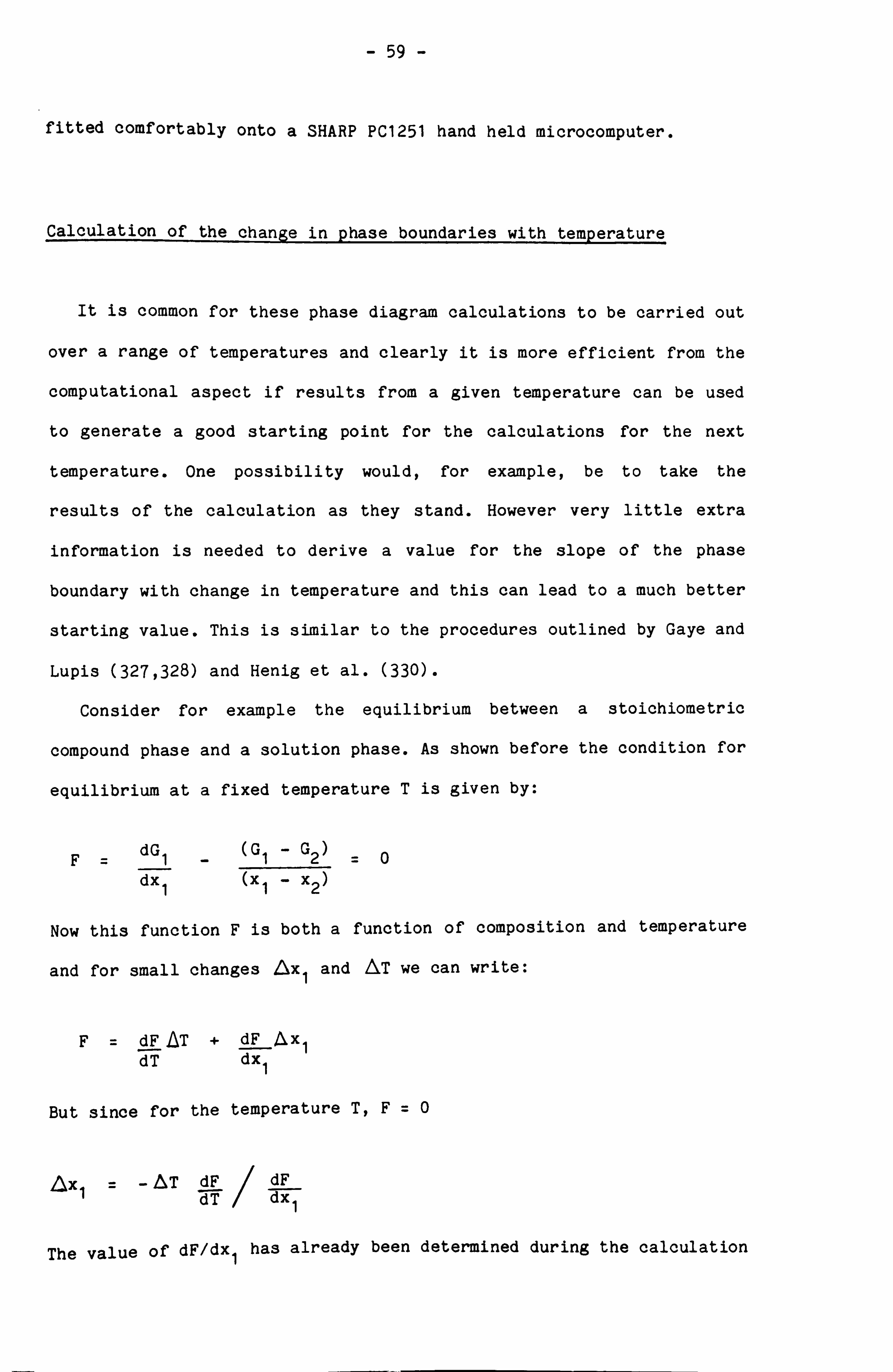
- 59 -
fitted comfortably onto a SHARP PC1251 hand held microcomputer.
Calculation of the change in phase boundaries with temperature
It is common for these phase diagram calculations to be carried out
over a range of temperatures and clearly it is more efficient from the
computational aspect if results from a given temperature can be used
to generate a good starting point for the calculations for the next
temperature. One possibility would, for example, be to take the
results of the calculation as they stand. However very little extra
information is needed to derive a value for the slope of the phase
boundary with change in temperature and this can lead to a much better
starting value. This is similar to the procedures outlined by Gaye and
Lupis (327,328) and Henig et al. (330).
Consider for example the equilibrium between a stoichiometric
compound phase and a solution phase. As shown before the condition for
equilibrium at a fixed temperature T is given by:
F_ dG1 -
(G1 - G2)
dx1 (x1 - x2)
Now this function F is both a function of composition and temperature
and for small changes Axt and AT we can write:
F= dF AT + dF Ax1 dT dx1
But since for the temperature T, F=0
A, x1 AT dF dF dT dx1
The value of dF/dx1 has already been determined during the calculation
- 60 -
of the equilibrium whilst dF/dT can easily be obtained from knowledge
of the variation of the thermodynamic data with temperature.
In a similar way, for the equilibrium between two solution phases
we have two equilibrium conditions both of which are functions of x, ,
x2 and T.
ie. F dG1 -
(G1 - G2) ý
dx1 (x1 - x2)
and F2 = dG2
- (G1 - G2)
_0 dx2 (x1 - x2)
For small changes in T, x1 and x2 we can write:
F1 = dF10T
+ dT
dF Ax1 + dx1
dF2 Lxs + dx1
dF 1 Ax
22= d x2
dF2 bx2 =0 dx2
F2 = dF2 AT + dT
It can be shown that
dF1 =
F2
dx2 (x1-x2) and
dF2 =
F1
dx1 ( x2-x1 )
which are both equal to zero since for the temperature T, F1 and F2
equal zero. Therefore again we obtain:
Axt _ -AT dF1 dF1
dT dx1
0x2 AT dF2 dF2
dT dx2
The quantities dF1 /dx1 and dF2/dx2 are known from the equilibrium
calculations while dF1 /dT and dF2/dT can be derived from a knowledge
of the temperature dependence of the thermodynamic data.
Using these expressions good initial guesses can be derived for

- 61 -
equilibrium calculations at a new temperature. This will speed up the
overall calculation of the phase diagram.
Procedure for the calculation of stable phase boundaries at a fixed
temperature
There have been three main methods used for calculating a complete
binary phase diagram. Kaufman (46) has preferred to calculate all
possible equilibria over a wide range of temperatures and then
identify those equilibria which are stable. An alternative method used
by Ansara (79) in his program BINAIRE is to calculate for each
temperature all the stable two phase equilibria by determining the
combinations of phases across the binary system which give the lowest
Gibbs energy. Jansson (292) has developed a third method within his
general program POLY whereby a given phase boundary is followed
automatically until it is found to be unstable with respect to some
new equilibrium or a pair of equilibria. These new equilibria are
followed in turn. In this way all stable phase boundaries which are
topologically linked can be determined.
For this work a similar approach has been adopted to that used by
Ansara (79). The intersections between stable solution phases are
calculated in order to define the lowest Gibbs energy curve against
composition from the various individual solution phases as shown in
Fig 5.4. At this stage each solution phase is scanned for pairs of
points of inflection which indicate tendency towards immiscibility.
The Gibbs energy of each of the stoichiometric compound phases is then
compared with that of the stable solution phase at that composition.
Then using the methods described in the last section, phase equilibria
are calculated between the intersecting solution phases, and between

LJ
0 Q"
"IIi
"" " ""
""
- "
., " . " "
".
" " " ,
"
." ", " " ,
" " "" "" " " . " ", " , " ,. ",.
" .""
"" ". ,
", ,
" " -, " ."
"
A 0.20 0.40 0.60 0.80 6
X --ý
B
Fig 5.4 Lowest Gibbs energy profile for various intersecting solution phases.
m
-1088
-2008
-3808
-4888
-5080
-6000
=7088

- 62 -
stable compounds and the solution phase stable at that composition as
shown in Fig 5.5. For each solution phase the equilibrium composition
is noted. If the calculated phase boundaries for a given solution
phase overlap, this phase is then unstable relative to a two phase
region between the two other phases as shown in Fig 5.5. For
equilibria involving stoichiometric compounds the Gibbs energy
gradient is noted. If two such gradients for a given compound indicate
a concave Gibbs energy envelope the compound will also be unstable as
shown in Fig 5.6. New phase equilibria are then calculated and
compared in turn with neighbouring equilibria until a set of
consistent phase boundaries have been obtained for the whole
composition range.
Any possible miscibility gaps then have to be tested against this
set of equilibria. A miscibility gap is calculated for each solution
phase with inflections provided that the phase had been calculated to
take part in the set of stable equilibria. For each of these
miscibility gaps then, the phase boundaries of this phase lying within
the region of immiscibility are counted. If there are none and the
phase had also been calculated to be stable within this region, the
miscibility gap is stable and must be entered accordingly into the set
of stable equilibria as shown in Fig 5.7. If the number of phase
boundaries is found to be one the miscibility gap is metastable and
furthermore, a metastable solution had previously been calculated to
be stable as is shown in Fig 5.8. A new calculation of this same
equilibrium is required but with the two phase region stretching
across the metastable miscibility gap. Finally if two phase boundaries
were found to be within the miscibility gap, the phase will no longer
be stable. A new calculation of equilibrium is required between the
two phases on either side of the metastable miscibility gap as shown

n4
-1888
-2088
-3888
-4800 4
-5000
-6000
-7000
t \ 'N V
\ ' N V
f
\
A 0.20 0.40 0.60 0.80
x --ý B
Fig 5.5 Calculation of phase equilibria between two intersecting solution phases and between a compound phase and stable solution phase. The phase boundaries for one solution phase overlap indicating that the phase is unstable relative to a two phase region.
B
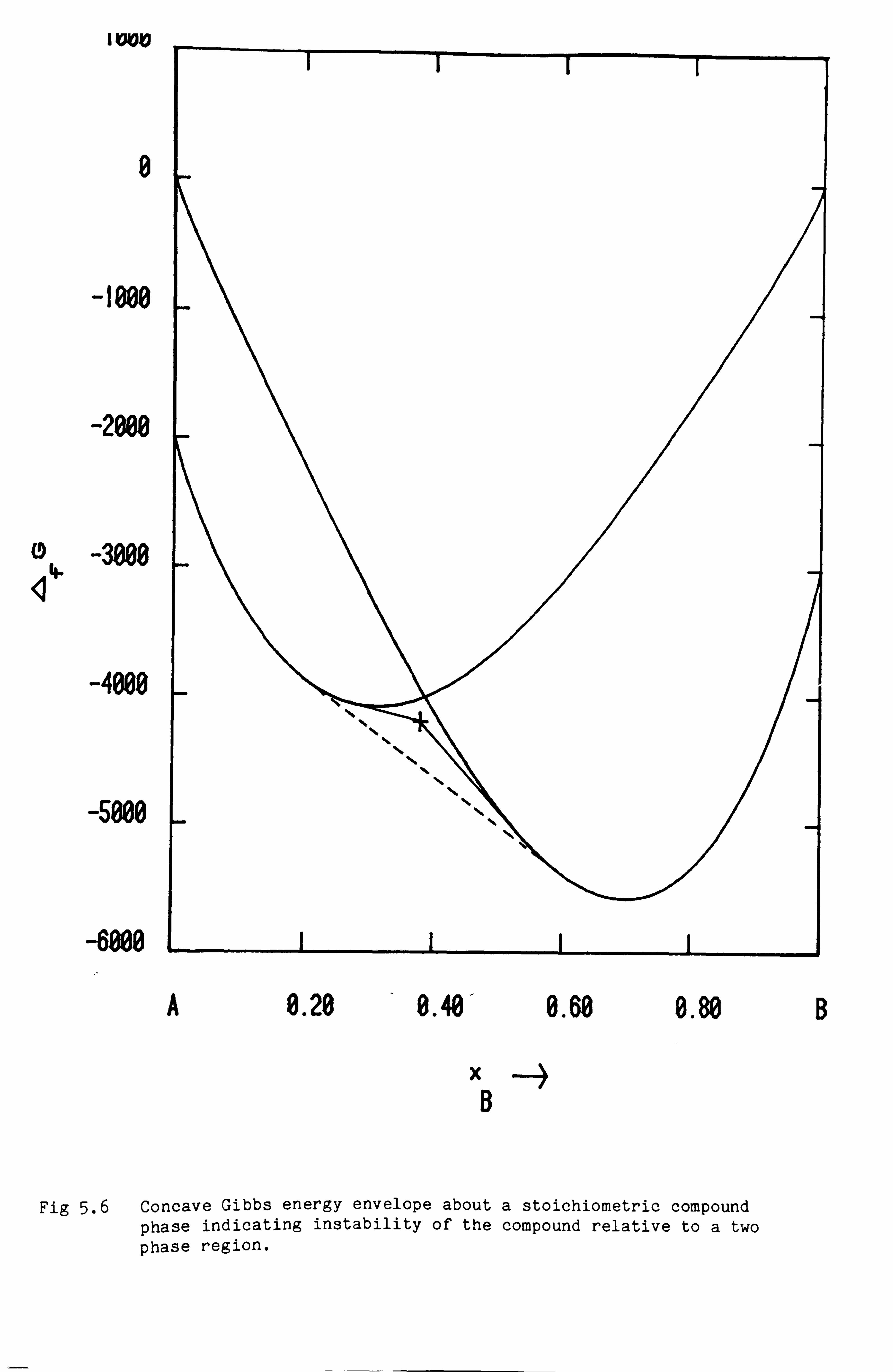
Ioolo
8
-1000
-2088
-3808 4
-4000
-5000
-6000
1
A 0.28 8.48
x 6
0.60 0.80 B
--4
Fig 5.6 Concave Gibbs energy envelope about a stoichiometric compound phase indicating instability of the compound relative to a two phase region.

O
4 ý
ýý
-400
-see
-800
-1080
A 0.20 8.48 8.68 0.88 B
xý B
Fig 5.7 Stable miscibility gap.

-288
O 1II.
-4A
-M
-800
-1008
_ -- -_
ýý
A 8.28 . 0.48,
x B
0.60 0.88 B
-4
Fig 5.8 The calculated miscibility gap is metastable relative to a two phase region between this phase and another phase spanning the region of immiscibility.
- 63 -
in Fig 5.9. In these last two cases (Fig 5.8 and Fig 5.9) the new
phase boundaries could result in an overlap of compositions for a
solution phase as in Fig 5.5 or a concave Gibbs energy envelope as in
Fig 5.6. This must be identified and equilibria recalculated where
appropriate.
Conclusions
In principle a number of methods can be used to calculate phase
equilibria in binary alloy systems. In this present work a procedure
based upon the Newton-Raphson technique has been developed. The method
is efficient, reliable and compact. This method has also been extended
in order to predict the effect of temperature on the phase boundaries
and this allows very efficient calculations of equilibria over a range
of temperature. A procedure has also been developed to calculate
automatically the stable phase boundaries for a binary system at a
given temperature. This procedure can be repeated for a series of
temperatures allowing the calculation of the whole phase diagram. Fig
5.10 and Fig 5.11 show examples of phase diagrams calculated
automatically using this program.

-288
O 1II.
400
-M
-ý
-1008
A 8.20 0.40 0.60
X -ý B
8.88
Fig 5.9 The calculated miscibility gap is metastable relative to a two phase region between two other phases spanning the region of immiscibility.
B

1500
11 363
1300
c N
0)
1 Liquid
0+
cph
617
582
11801
4
1100
900
700
Son
Vapour
M CN
CNC NNN m 0) 0)
861
0
689
621
618
657
C^ N
N 0)
1
644
cph
Mg 0.2 0.4 0.6 0.8 Zn
x Zn
Fig 5.10 Phase diagram for the Mg-Zn system calculated automatically using the binary phase diagram program. The experimental phase equilibria have been superimposed.

1500
1300
1100
U 0
900
700
X
O
V + O
0 " A
Roberts Calculated Craighead al. jej. Kobayashi et al. Berthon et al. Broniewski and Smialowski Fraenkel Batalin et al. X Singer and Cottrell Dix and Heath Drits et al.
0
v
Liquid 0
o Liquid + Si(dia) 0
0
577
500 AI(fcc) + Si(dia)
300 Al 0.2 0.4 0.6 0.8 Si
X
Si
Fig 5.11 Phase diagram for the Al-Si system calculated automatically using the binary phase diagram program. The experimental phase equilibria have been superimposed.
- 64 -
CHAPTER 6
Thermodynamic Properties of Alloys in the
Fe-Ti System
Introduction
This work was the last of a series of experimental studies on
thermodynamic data for binary and ternary alloy systems of industrial
importance carried out at the National Physical Laboratory. The system
Fe-Ti was chosen because critically assessed thermodynamic data for this
system were needed for use in the calculation of multicomponent phase
diagrams (15,334). Ti is often added to stabilise stainless steels and
also acts as a deoxidant. Therefore information relating to its effect
on the phase diagrams of steel systems is particularly important. There
had however, been very little experimental thermodynamic work done on
solid alloys in this system upon which to base a critical assessment.
In addition, it was hoped to extend the range of the adiabatic
calorimeter used for previous measurements (335,336) to include more
exothermic alloy systems such as the Fe-Ti system. Previously the
systems studied were restricted to those in which the enthalpies of
formation were between about +8 kJ/mol.
The Fe-Ti phase diagram determined by experiment is shown in Fig 6.1
and is based on that presented in Elliott (54) but incorporates
experimental work referred to in Hansen and Anderko (53) and Shunk (55),
and work of Abrahamson and Lopota (337), Raub et al. (338), Nasu et al.
(339), Matyka et al. (340) and Ko and Nishizawa (341).
In the work described here, the enthalpy of formation was determined
for 5 different compositions: for xTi=0.05 which at high temperatures is
in the bcc phase field, for xTi = 0.10 and 0.20 which lie in the two

2000
180C
160C
1400
1200
1000
-Ti)
800
600 - Fe
xTi
Fig. 6.1 Experimentally determined phase diagram for the Fe-Ti system.
0.2 0.4 0.6 0.8 Ti
- 65 -
phase region between the Fe based bee solid solution and the Laves phase
compound Fe2Ti, and for xTi = 0.333 and 0.50 for the two compounds Fe2Ti
and FeTi respectively. Based upon these and other measurements of
thermodynamic properties a critical assessment was carried out to
provide data for the various phases in the system as a function of
temperature and composition. These critically assessed data are now
suitable for use in the calculation of multicomponent phase diagrams.
Experimental
The measurements were carried out using a high temperature adiabatic
calorimeter designed by Dench (26) and shown in Fig 6.2. The details of
its construction, operation, and of the preparation of specimens have
been described elsewhere (26).
The materials used in the experiments were 'carbonyl' iron powder,
and titanium powder supplied by ICI Mond division. The iron powder was
reduced under hydrogen at 630 K, ground in an agate mortar, and sieved.
The -400 mesh fraction was used in the experiments. The titanium powder
was also sieved, and the -300 mesh fraction used. The gas contents of
the powders, determined by the vacuum fusion method, are shown in Table
6.1.
The enthalpies of formation of the alloys were determined by
measuring the energy required to heat specimens between two chosen
temperatures. Two measurements were required to measure an enthalpy of
formation - a) one in which complete alloying takes place and b) one
where no alloying takes place. To make sure that the alloying occurred
only during the experiment and was complete by the end of the
experiment, preliminary tests were made to determine a 'safe'
temperature where no detectable alloying occurs even when the specimens
were held at this temperature for 4 hrs, and a 'final' temperature at

Internal heater
rhermoc
=urnace
Pater -cc ý acuum
Differential thermocouple
Specimen
adiabatic 'nclosure
Fig. 6.2 Schematic diagram of the adiabatic calorimeter.

Table 6.1. Mole fraction of impurities in the alloying materials from gas analysis.
x0 xN xH
Ti 0.0072 0.004 0.0081 Fe 0.0010 <3x10
6-
Table 6.2. Results of preliminary experiments to determine the 'safe' and 'final' temperatures.
XTi Sintering Constitution
temp /K time / hrs
0.04 873 4 Fe + Ti
973 4 Fe + Ti 1073 4 Fe + Ti + Alloy
1273 1 Fe + Fe2Ti
1373 1 Bcc Alloy
1473 1 Bcc Alloy
0.333 873 4 Fe + Ti
973 4 Fe + Ti 1073 4 Fe + Ti
1273 1 Fe + Ti
1373 1 Fe2Ti + FeTi (trace)
. 473 1 Fe2Ti
0.5 873 4 Fe + Ti
973 4 Fe + Ti 1073 4 Fe + Ti
1273 1 FeTi + Fe2Ti
1373 1 FeTi
1473 1 FeTi
0.95 873 4 Fe + Ti
. 973 4 Fe + Ti
1073 4 Fe + Ti
1273 1 Alloy + Fe2Ti (? )
1373 1 Alloy + Fe2Ti (? )
1473 1 Alloy + Fe2Ti (? )

- 66 -
which complete alloying took place in the specimens within 1 hour. The
specimens from these preliminary tests were examined both
metallographically and by powder x-ray diffraction and the results are
summarised in Table 6.2. Suitable temperatures were found to be 973 K
for the 'safe' temperature and 1473 K for the 'final' temperature.
Two different procedures were used to determine the enthalpies of
formation as can be seen from the following scheme:
xFe(T1 )+
FexTiy(Tý)
xFe(T1 )+
yTi(T1)
) ---ý yTi(T1
FeXTiy(T2) H1
FeXTiy(T2) H2
xFe(T2) + yTi(T2) H3
Here, T1 refers to the 'safe' temperature and T2 to the 'final'
temperature. The mole fractions of Fe and Ti are x and y respectively.
In this scheme, H1 refers to the energy change in the alloying
measurement while H2 and H3 refer to energy changes when no alloying
occurs. For measurements of H2, the specimen consisted of the alloyed
compacts from the previous measurement ie. for measuring HV This type
of measurement is called a 'repeat' run. For measurements of H3, the
specimen consisted of discrete compacts of the component elements of the
same weight and in the same overall composition as the alloying specimen
-a so-called 'composite' specimen. The compacts of Fe in the composite
specimen were separated from the Ti compacts by thin layers of Ta sheet
to prevent any alloying occurring at the surfaces.
When these measurements are combined it is possible to derive the
enthalpy of formation applicable to either the 'safe' temperature or the
'final' temperature.
ie. t H(FeXTiy , T1 )= H1 - H2
AfH(FeXTiy , T2) = H1 H3

- 67 -
Fig 6.3 shows a typical heating curve, in this case for an alloying
run. The specimen is heated up using the calorimeter furnace and
stabilised approximately at the 'safe' temperature. The heater is then
used to heat the specimen until the 'final' temperature is reached.
During and after the heating period, adiabatic conditions are maintained
by an automatic control system which responds to temperature gradients
across the adiabatic enclosure detected by differential thermocouples
(Fig 6.2). The final slope after the heater is switched off is
extrapolated back to a time mid-way through the heating period to
determine the exact final temperature. This allows for slight departures
from adiabatic conditions. The energy supplied to the heater is
corrected using measured heat capacity data around T1 and T2 to
determine the energy that would have been required to heat the specimen
from the precise 'safe' temperature to the precise 'final' temperature.
The sharp change in slope in the heating curve marks the onset of
alloying. Figure 6.3, which refers to the formation of an alloy with
xTi=0.10, shows this change in slope at about 1300 K which is
approximately the eutectic temperature in the Ti rich side of the phase
diagram.
Two factors make measurements difficult when alloying is very
exothermic. Firstly, a large quantity of heat is evolved in a short
time, too much for the automatic system of the calorimeter to control,
causing the loss of adiabatic conditions. Secondly the large amount of
heat evolved would produce a large temperature rise. The final
temperature might then be so high that the specimen would melt or the
calorimeter would be outside its safe operating range. In general, the
calorimeter is restricted to temperatures below 1600 K.
In order to overcome these problems, it was necessary to reduce the
quantity of heat evolved per gram of specimen.

1600
1400
1200
Y
H-
1000
800
600
Heater switched off T2ý-__
Main reaction starts
f
T,
20 40 t /min
60 80
Fig. 6.3 Typical heating curve for an alloying run.
- 68 -
Fig 6.4 shows the method used where the alloying compacts were separated
by discs of molybdenum which acted a heat sink. This method proved to be
very effective. However the errors in measurement were inherently much
greater than for previous sets of experiments since less alloying
material was used per specimen. This showed up in the scatter of the
experimental results as shown below.
Results and Discussion
Table 6.3 shows the results obtained for the Fe-Ti system for each of
the compositions studied. The derived enthalpies of formation are
plotted as a function of composition in Fig 6.5 for 973 K and in Fig 6.6
for 1473 K. The estimated accuracy of the / fH values, which varies
according to the degree of dilution, is shown as errors bars in the
figures. These results clearly show the exothermic nature of these
alloys. It is difficult to compare the two curves for the enthalpy of
formation however since they refer to different reference phases for the
pure elements and also because the bcc/(bcc+Fe2Ti) phase boundary varies
appreciably with temperature.
There have been four other sets of measurements on solid alloys in
the Fe-Ti system. Kubaschewski and Dench (342) measured the enthalpies
of formation of the two compounds. They obtained for FeTi a value of
-20.3 +3 kJ/mol at 298 K. The present work shows that the enthalpy of
formation for 973 K is -29.9 +3 kJ/mol. This is of the order of 7-9
kJ/mol more exothermic than Kubaschewski and Dench's value even if one
allows for a difference of heat capacity between products and reactants
of up to 4J mol-1 K 1. This discrepancy is almost certainly due to
Kubaschewski and Dench's calorimetric method where considerable heat
loss was likely.
Kubaschewski and Dench also attempted to measure the enthalpy of
formation of Fe, Ti. They obtained the value of -19.0 +2 kJ/mol but were
Heater cavity
Molybdenum disc heat
sinks
Compacted reaction mixture
(um ipsute
Fig. 6.4 Schematic layout of alloying specimen. Alloying compacts are separated by molybdenum discs.
Thermocouple well

H 1U %lo A 0 00 M O M 00 u1 -It N O\ N N- '. O ". )C
N l` 00 . Ll- \D 00 _ Lr. '-O M %1D 4- ON v CO . d' N- 0
H E
00 f
(V O' N o0 00 " M
" " Ö " " "
- " "
T- "
r- " " 0 - l 1 00 00
r (V N 00 O ON -t . A 1
4- 0 0
P. + Oý r ýI T-
t4ý K l\ \D N
Q\ 4-
N. N N O, O N LA \. D M N N ä I I I
M - It\ 00 - .ý N L. 00 N N N N N M N N N U
1 I I $ I 1 I I I 1
VI\ 00 O 4- 00
0 T- . .
' .
19 & N 00 Lf \
N N 4- 4-
L M M N N 4) ri N N N 0
I` N M --t r4 \
O- 00 N l0 .f N
r .. 0
. N N tN O N.
O \ , E a' e- - r
- r- N \10
r ý10 r
%10 r cl- N
N N
U 4- - -: f
4- 4-
N N N T" r- T-
., a H
r" IV N. N
0 ýN 00
LA ONO a' Lr\ N M 00 - Ll- N. a'
ca N CO N. N . Cý E-4 0 O N .
O' O oo .
p' . oo
. N . -. p .
N . 0 .
Q\ . .
ýp .
%Z C- 11A .
oo N x pý M ýD O 00 00 M O zt- Cý OD O\ -* O M O' a' M v- N O r N v- lfl pý N. 4- . - -- p' L- L. VIA N Ul C. N. 4+ W N Ul 111 L O N N v a M 0 0 4- C. 00 N- <1\ I 1 I 1 1 1 T- rl- c- rl- r N N N N N N N V 1 I I I I I I
V 0
cc 0 a' r" Oý
O 4-
LrIA
1A u1 O
00 L`
\lD N
ul g . - L- C- O' I
ON %Z ON 0 0
u1 tL 0 I
0 ON 4- 'O U1 a' M u1 C` M N M "rl J
+' \ N
LA llý . .
1'f\ "
r- .
0 .
tM .
. - M .
c- .
ON c- .
V- c- .
0 r
Cý 00
1+1 N. N
4- N
Q' O
N N
CO \O 00 r -- CN
00 ca
r- 00
M 00 L ON u\
4- cc
-- . - 4- 4- 4-
4- M M M 00 111 '. D \1O ON %O ä N N N N c- v v- c- v" v- c- . v v . v Lr\ r 4 r
-t N a\ N r r
4-3
F N t l ON N -
CI N 00 In v- N
u c- .
l r' . 0
do "rl " . . l N N N. -t N 00 %. D to 0 0
f~ I7 .
Oý Ul e0 Oý M r Cý M L
00 00
LA N. \. D r N
4p FD N 00
ýD r M
o0 00 Ö i N 00 N r Ö O :t 0 . i i M prý 0 00 O O O O1,
0 N N M
KA N Hr-I N N N N r r r r r r r r r r r r r r
aw
M M M M M M M M M M K1 M M M M M M M M N Cl- S r am am am r r r r H r r r r r r r r r c - c - - c
M t-
Pal N
IA N.
M N.
IA N.
Ký L`
M N-
M N.
M [-
M N.
M N
f+1 N
M L-
M [-
M M M M M Q\ O\ ON O' O\ Q' O\ O' ON O1\ O' O' O' O' O\ Q'- Q' Q' O'
H
si
Ö In 4- -: I- N- p' u1 \O . - 4- ON Cl- N. M LA ul v 00 v 0
rl -P O N
0 N1 00 00 00 N. N
C. N N
'. p N
pp h0
M M M M r r
00 ON
° co
CT\ 0
a, N N N N
. . . . . . . . . . . . . . 4-1 E ýO l
u1 l
v- Ir- v- u1 u1 LA ul 00 00 00 00 .
CO . N . N .
N. .
C. O0 U\ U \ Lf \ t11 Ul\ l. A ' r r
4
0 N >a r-
p R
O 8 O p O
H
M
H
G 6-1
C7
ßr a
ýa
G) p F
1
O E
Y
d
-40
-30
-20
-10
0
973K II
- Present work
X Kubaschewski and Dench
III II
III
f
I ýI I
III IIý 1I III
IIý III
bcc [Fe2TI' FeTi
0 Fe
0.2 0.4 x Ti
0.6
Fig. 6.5 Experimental enthalpies of formation for 973 K from bcc Fe
and hcp Ti.

_Ir
O E
I
Q
fcc
xTi
Fig. 6.6 Experimental enthalpies of formation for 1473 K from fcc Fe and bcc Ti.
Fe 0.2 0.4 0.6

- 69 -
suspicious because they had expected to find that A. fH(Fe2Ti) would be
more negative than AfH(FeTi) in view of the erroneously high melting
point then accepted for Fe2Ti. On investigation they found however, that
during their experiments the reaction produced a mixture of FeTi and the
bcc iron based solid solution rather than the expected Fe2Ti.
The present measurements gave -21.3 + 2.5 kJ/mol for AfH(Fe2Ti) at
973 K, a value quite close to that obtained by Kubaschewski and Dench.
From the preliminary experiments described earlier, and summarised in
Table 6.2, it was found that Fe2Ti forms completely when the specimens
are held at 1473 K for one hour, and with a small quantity of FeTi only,
when they are held at 1373 K for one hour. Furthermore, an X-ray
examination of an alloying specimen revealed that Fe2Ti had been formed
completely. The fact that Kubaschewski and Dench formed only a mixture
of FeTi and bcc may be attributed to the much larger particle size of
the material they used which would have caused much slower alloying.
The enthalpies of formation of the two compounds have also been
studied by Gachon et al. (343-345) subsequent to the present
measurements. They obtained values of -31.0+1.3 kJ/mol for FeTi at
1440 K, and -27.6+1.0 kJ/mol for Fe2Ti at 1514 K. Their results imply
even more exothermic behaviour than implied by the results obtained
during the present work and they also confirm that the enthalpy of
formation of FeTi is more negative than that of Fe2Ti.
The enthalpies of formation for both of these compounds have been
calculated by Miedema and Niessen (346) using their semi-empirical
electronic model, and for FeTi by Watson and Bennett (347). Both sets of
predictions give results in remarkable agreement with the present
experimental results (within 1 kJ/mol).
Palma and Schroder (348) reported high temperature heat capacity
measurements of iron-rich alloys between 600 and 1150 K in the region of

- 70 -
the magnetic transformation. They found that the heat capacity and the
Curie temperature were effectively independent of the amount of titanium
for compositions up to xTi = o. o48.
Robinson and Argent (349) used Knudsen cell mass spectrometry to
determine the partial enthalpies, excess partial Gibbs energies and
excess pErtial entropies of solution at about 1600 K. Their values for
the partial enthalpies of mixing agree well with the enthalpies of
formation reported here. It should however be pointed out that their
enthalpies were derived from the temperature dependence of vapour
pressure measurements, a method subject to large errors.
A number of thermodynamic studies on the iron-titanium system have
been concerned with the liquid phase. The results of Wagner and St.
Pierre (350) for 1818 K and Furukawa and Kato (351) for 1823 K and
1873 K from Knudsen cell mass spectrometry show that the liquid phase
can be represented approximately as a regular solution. However there is
significant disagreement between the Gibbs energies of formation derived
from the two sets of experimental ion intensities - the results of
Furukawa and Kato (351) implying more negative Gibbs energies of
formation.
A number of workers have studied the deoxidation equilibrium of iron
at low titanium concentrations and derived the titanium activity
coefficient at infinite dilution (352-357). Their results are summarised
in Table 6.4 and compared with the ö Ti values obtained from the results
of Wagner and St. Pierre (350) and Furukawa and Kato (351). The results
reported by Fruehan (356) and by Smellie and Bell (357) refer to a
reference state of pure solid titanium. The titanium activity
coefficient at infinite dilution was derived by Fruehan from
extrapolation of activities at various titanium concentrations.
The ion current ratios reported by Wagner and St. Pierre (350) and
Furukawa and Kato (351), have been used to derive activities and

Table 6.4. Experimental values for the Activity coefficient, 1Ti at infinite dilution.
Authors Method Temperature /K Ti
Chipman (352) from results of Hadley Deoxidation 1900 0.011 and Derge (353)
Chino et al. (354) Deoxidation 1823 0.020 1873 0.033 1923 0.060
Suzuki and Sanbongi Deoxidation 1873 0.016 (355)
Fruehan (356) * EMF 1873 0.038
Smellie and Bell Deoxidation 1973 0.059 (357)
Wagner and St. Mass Spec. 1818 0.056 Pierre (350)
Furukawa and Kato Mass Spec. 1823 0.022 (351) 1873 0.024
* Refers to reference state of bcc Titanium

- 71 -
activity coefficients for the whole composition range. Fig 6.7 shows a
plot of the activity coefficient of titanium (referenced to liquid Ti)
converted to 1873 K for all the results on this liquid phase. The figure
shows a marked difference between the two sets of mass spectrometric
results and this is emphasised in Fig 6.8 where the integral excess
Gibbs energies at 1823 K derived from these activity coefficients are
plotted. Fig 6.7 also shows that the deoxidation data agree better with
Furukawa and Kato's results than with those of Wagner and St. Pierre.
For this reason and because they also agree well with the present
enthalpy measurements, the results of Furukawa and Kato were preferred
for use in the critical assessment.
Dyubanov et al. (358) measured calorimetrically the partial enthalpy
of solution of Ti in liquid iron as -52.0 +3 kJ/mol at 1823 K.
Critical Assessment
The thermodynamic data for this system have been assessed previously
by Kaufman and Nesor (359) using a subregular solution model for the
liquid, bcc and fcc solution phases and assuming that the compounds
Fe2Ti and FeTi were stoichiometric. Because of the new measurements this
assessment is now superseded.
Since this present work was completed the phase diagram and the
thermodynamic data for the Fe-Ti system have been critically assessed by
Murray (360). In her assessment she preferred the data of Wagner and
St. Pierre to those of Furukawa and Kato and also had no access to the
recent experimental measurements of the enthalpies of formation of solid
alloys. The liquid, fcc, bcc and hcp phases were represented by regular
or subregular solution models with no temperature dependence for the
parameters. However she used different descriptions for the Fe rich bcc
phase and the Ti rich bcc phase. The two compounds were represented as

>~
.'
xTi
Fig. 6.7 The variation of activity coefficient of titanium for 1873 K derived from experimental measurements.
Fe 0.2 0.4 0.6 0.8 Ti

0
Furukawa and Kato
Wagner and St Pierre
r-
O E
. ýC
ýIJ 0 Q
-5
-10
-15
-20 Fe 0.2 0.4 0.6
x Ti
0.8
Fig. 6.8 Integral Gibbs energies of formation for 1823 K derived from
experimental results of Wagner and St. Pierre (350) and Furukawa and Kato (351).
Ti

- 72 -
Wagner Schottky phases with iron and titanium sublattices. Vacancies
were introduced onto the titanium sublattice while titanium atoms were
assumed to substitute onto the iron sublattice. Very good agreement was
obtained between the calculated and experimental phase diagram except
that she failed to reproduce the peritectic fusion of FeTi.
For the present critical assessment it was decided that the liquid,
bcc and fcc phases should be represented by Redlich-Kister power series.
The solubility of Fe in the hcp phase, which is known from experiment to
be very low (338-340), was neglected and the phase was treated as
stoichiometric. In a similar way the compound FeTi, which exists over a
narrow range of homogeneity was treated as a stoichiometric phase. The
Laves phase compound Fe2Ti exists over a fairly wide range of
homogeneity. For this assessment its data were represented by a
Redlich-Kister power series. This approach had already been used with
some success for the Laves phase compounds Co2Zr and Cr2Zr (361) and
with the treatment of sigma phases (167,362).
For this assessment all data were referred to pure bee Fe and pure
bce Ti at the temperature of interest. The fusion data for Fe (bcc to
liquid) were taken from Hultgren et al. (43) and for Ti (also bcc to
liquid) from the experimental work referred to in Hultgren et al. (43),
and the work of Berezin et al. (363). Data for the Gibbs energies of
transformation for the pure elements from the bcc phase to the fcc and
hcp phases were taken from Kaufman (364). It was also necessary to
estimate data for the hypothetical transition bcc to Laves for both of
the elements. These Gibbs energies of transition were taken to be
temperature independent in the absence of any other information.
Using the measured enthalpy of formation for the Laves phase at
xTi = 0.333 for 1473 K, the Gibbs energies of formation of the liquid
phase at 1873 K derived from the experimental measurements of Furukawa
and Kato (351) and the congruent melting temperature of the Laves phase

- 73 -
compound at 1700 K, the entropy of formation for. the liquid and the
Laves phases at xTi = 0.333 were estimated. This was subject to the
constraint that the entropy of formation be compatible with the known
empirical relationship between enthalpies and excess entropies of
formation (365) and, in addition, that the entropy of fusion of the
compound is less than that for an order to disorder transformation. The
data now derived for the liquid phase were found to be in good agreement
with the partial enthalpy of titanium at infinite dilution in liquid Fe
measured by Dyubanov et al. (358).
From these assessed data, data for the Laves phase as a function of
temperature and composition were derived to reproduce as closely as
possible the experimental phase boundaries between the Laves phase and
the liquid phase. The calculated phase width is, in terms of mol
fraction, about 0.04 greater than that determined experimentally.
The compound FeTi melts peritectically at about 1590 K. Using the
enthalpy of formation data reported here, an entropy of formation was
derived to reproduce the known fusion behaviour.
Data for the bcc phase were derived in order to reproduce the
experimentally determined eutectics at xTi = 0.16 and at xTi = 0.71 (see
Fig 6.1. ) using the activity data of Robinson and Argent (349) but
keeping approximately the same excess entropy curve as for the liquid
phase. The agreement with the experimental phase diagram is good at high
temperatures as shown in Fig 6.9. At low temperatures, however, the
agreement is less satisfactory and the calculated eutectoid between the
bcc, hcp and FeTi phases at high titanium concentrations is about 230 K
lower than experimentally determined. This is probably due to the use of
an inappropriate model for the Laves phase resulting in its calculated
homogeneity range being too large, linked with the absence of heat
capacity data for FeTi which could introduce significant errors over,
say, 1000 K. The experimental and selected enthalpies of formation are
2000
1800
1600
1400
10.00,
1200
1000
-Ti )
800
600' Fe
x Ti
Fig. 6.9 Phase diagram for the Fe-Ti system calculated from the
critically assessed thermodynamic data.
0.2 0.4 0.6 0.8 Ti
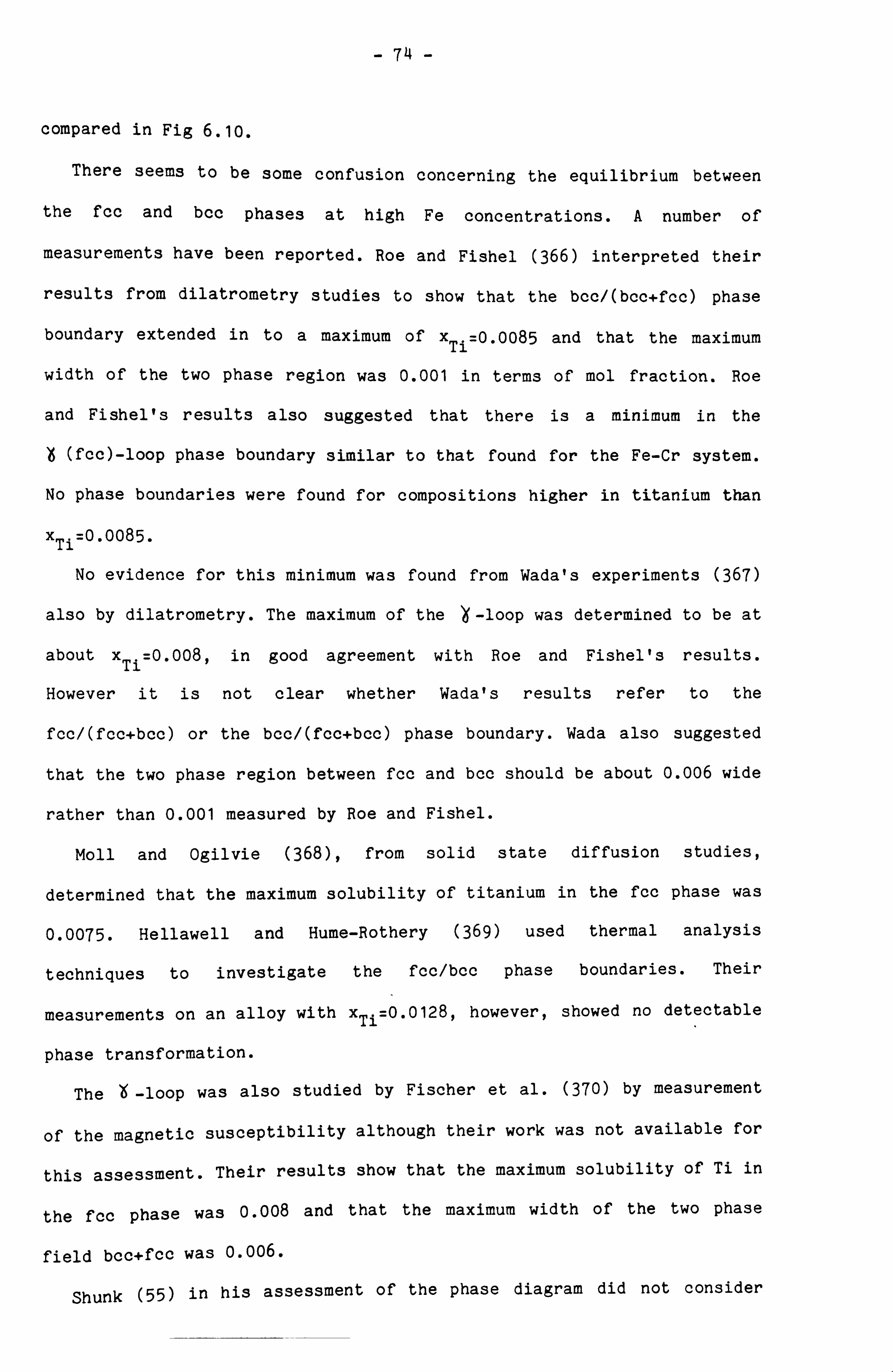
- 74 -
compared in Fig 6.10.
There seems to be some confusion concerning the equilibrium between
the fcc and bcc phases at high Fe concentrations. A number of
measurements have been reported. Roe and Fishel (366) interpreted their
results from dilatrometry studies to show that the bcc/(bcc+fcc) phase
boundary extended in to a maximum of xTi=0.0085 and that the maximum
width of the two phase region was 0.001 in terms of mol fraction. Roe
and Fishel's results also suggested that there is a minimum in the
t (fcc)-loop phase boundary similar to that found for the Fe-Cr system.
No phase boundaries were found for compositions higher in titanium than
xTi=0.0085.
No evidence for this minimum was found from Wada's experiments (367)
also by dilatrometry. The maximum of the ' -loop was determined to be at
about xTi=0.008, in good agreement with Roe and Fishel's results.
However it is not clear whether Wada's results refer to the
fcc/(fcc+bcc) or the bcc/(fcc+bcc) phase boundary. Wada also suggested
that the two phase region between fee and bee should be about 0.006 wide
rather than 0.001 measured by Roe and Fishel.
Moll and Ogilvie (368), from solid state diffusion studies,
determined that the maximum solubility of titanium in the fcc phase was
0.0075. Hellawell and Hume-Rothery (369) used thermal analysis
techniques to investigate the fcc/bcc phase boundaries. Their
measurements on an alloy with xTi-0.0128, however, showed no detectable
phase transformation.
The ö -loop was also studied by Fischer et al. (370) by measurement
of the magnetic susceptibility although their work was not available for
this assessment. Their results show that the maximum solubility of Ti in
the fcc phase was 0.008 and that the maximum width of the two phase
field bcc+fcc was 0.006.
Shunk (55) in his assessment of the phase diagram did not consider
It J
O 0 0 X 0
H
O N
LL H LL
5 0
1 1 x
o 0 \x
5
Assessed Of H for bcc
alloys, assumed temperature X
0 independant from 1000- 2000K
5 o Present work 1473K x Present work 973K
Assessed AfH for stable 0 alloys. The phase boundaries
0 are for 1473K
x
0
x
FP 0.2 0.4 0.6 0.8 T; xTi
Fig. 6.10 Comparison of the experimental and selected enthalpies of formation for 1473 K.
II

- 75 -
the work of Fischer et al. and suggested that the maximum solubility of
Ti in the fcc phase should be 0.002. For this work the phase diagram
implied by Shunk has been adopted and data were derived for the fcc
phase to reproduce this diagram. It was also assumed that the
temperature dependence and asymmetry of the excess Gibbs energy curve
for the fcc phase is similar to that for the bcc phase. Fig 6.11 shows
the calculated ö -loop phase boundaries with some of the experimental
data superimposed. In the more recent assessment, Murray (360) adopted
the data of Fischer et al. for her assessment of the ö -loop equilibria.
Table 6.5 shows the critically assessed data for the Fe-Ti system.
Fig 6.12 shows a plot of the Gibbs energy of formation for each phase at
1600 K.
Summary. and Suggestions for Future Work
The thermodynamic data for the Fe-Ti system have been critically
assessed to be as consistent as possible with the accepted phase
diagram. The assessed data are now suitable for use in the calculation
of multicomponent alloy phase diagrams. This assessment, which was
carried out without the use of optimisation programs such as the one
developed by Lukas et al. (290,310), has one or two minor
inconsistencies compared with the diagram now accepted, notably the
extension of the ' -loop into the binary system, the homogeneity range
of the Laves phase and the eutectoid temperature at high titanium
compositions.
The more recent critical assessment of Murray (360) is in rather
better agreement with the accepted phase diagram although it is based on
experimental thermodynamic data which have now been superseded and which
differ significantly from values considered now to be correct. Murray
also used two different descriptions for the thermodynamic data for the

170
160,
JI
® Hellawell and Hume-Rothery
o Roe and Fishel
®I Wada
150
0
140
130
120
0
110
1000' Fe 0.002 0.004 0.006 0.008
xTi
Fig. 6.11 Theö-loop for the Fe-Ti systea calculated from the critically assessed thermodynamic data and compared with the
experimental results.
(y-Fe) (Y+a) (a- Fe)
0 0
If oII o0
O JIQ
i
It 8®
0.01

1080
0
-1000
-2088
-3888
-4000
-5080
-6009
-7080
Fe-Ti 1680 K
bccý
fcc .ý
Laves Liquid
t
Li
0.00 0.10 0.20 0.30 8.40 0.50 0.60 0.70 8.80 0.90
xTi
1.0ý
Fig. 6.12 Gibbs energy of formation as a function of composition for the different phases of the Fe-Ti system for 1600 K calculated using the critically assessed data.

- 76 -
bcc phase - one for iron rich compositions and one for titanium rich
compositions. Her assessment is therefore difficult to use in
multicomponent phase diagram calculations. In addition her data do not
reproduce the peritectic fusion of FeTi.
The model used by Murray to represent the composition dependence of
the Laves phase is more realistic than the Redlich-Kister expression
used in the present calculations. She represented the non-stoichiometry
of Fe2Ti in terms of a Wagner Schottky model with vacancies introduced
onto the titanium sublattice to explain deviations to iron rich
compositions, and titanium atoms substituting into the iron sublattice
to explain deviations to titanium rich compositions. In practice, of the
six types of point defects allowed, only the introduction of
interstitials will not take place to any appreciable extent in these
highly ordered Laves phases. The other four point defects - substitution
on each of the sublattices and the introduction of vacancies on each of
the sublattices should occur to some degree. In the case of the Fe2Ti
Laves phase, the homogeneity range is large to compositions iron rich of
Fe2Ti while it is fairly small except at high temperatures to titanium
rich compositions. In view of the slightly larger size of titanium atoms
the most important defects could be expected to be substitution of iron
atoms onto the titanium sublattice and the intoduction of vacancies on
the iron sublattice. This is different description from that adopted by
Murray.
It is recommended that the thermodynamic and the phase diagram data
be reassessed at some stage using an optimisation program. Such an
assessment should also include new data for the pure elements, a
treatment of the magnetic contribution to the thermodynamic properties,
data to represent the solubility of Fe in hcp Ti and the use of more
realistic models to represent the composition dependence of the
thermodynamic data for the Laves phase and FeTi.

lade 6.5
ASSESSED DATA FOR THE IRON-TITANIUM SYSTEM
I Solution Phases
The Gibbs energy of formation of a binary alloy from its component
elements in their reference phase is given by the following expression
LfG= OtG + GE + LGideal
where AtG is the Gibbs energies of transformation of the elements from E their reference phases to the phase in question, G is the 'so-called'
excess Gibbs energy and LGideal is the ideal contribution to the Gibbs
energy of formation given by the expression:
LGideal = RT (x in x+y In y)
where R is the gas constant, T the temperature and the alloy is of
composition AXBy .
a) Gibbs energies of transformation for elements in J mol 1
Element Transformation AtG -a+ bT + cT2 + dT3
a b c d
Fe bcc --ý Liquid 13807.2 -7.6316 0 0 bcc -ý Laves 5020.8 0 0 0
b cc ---ý bcc 0 0 0 0
bcc --ý fcc 5235.02 -9.4006 5.2949 x 10⁻³ -9.2215 x 10⁻⁷
Ti bcc --ý Liquid 13807.2 -7.1128 0 0
bcc -- Laves 8368.0 0 0 0
bcc -- bcc 0 0 0 0
bcc --> fcc -1004.16 3.7656 0 0

b) Coefficients for excess Gibbs energy of formation for the Fe-Ti system
The excess Gibbs energy of formationin J mol-l is given by:
GE XFeXTi [a + bT
+( 'e xTi)(a1 + b1T)
+ (xFe xTi)2(a2 + b2T)
+ (xFe - xTi)3(a3 + b3T)
+ (xFe x'I'i)4(a4 + b4T) ]
ab
Liquid -88453.76 17.5529 -3364.64 0
'0 0 o 0 o 0
Laves -123498.31 30.9428 -78573.89 19.6870 27913.70 -6.9940 65733.98 -16.4699 66038.13 -16.546o
bcc -69036.00 17.5529 -4184. oo 0
0 0 0 0 0 0
fcc -52300.00 17.5728 -4184. oo 0
0 0 0 0 0 0
2 Compound Phases
For compounds the Gibbs energy of formation from the elements in their
reference phases is given by:
AfG= a+bT+ cT InT
Compound xF, e xTi a b c
FeTi 0.50 0.50 -28660.40 4.1112 ! 0
_77_
CHAPTER 7
Quantitative Equilibrium Calculations
for Steel Systems
It was shown in chapter 6 how thermodynamic data for the
iron-titanium system were measured and used in a critical assessment- to
provide data for the various phases of the system which could be used in
the calculation of multicomponent phase diagrams. In chapter 4a variety
of computer programs were discussed which were developed for the
calculation of phase equilibria. In this chapter data and programs are
linked in order to provide quantitative calculations of phase equilibria
of importance to industry for steel systems.
The first set of calculations were undertaken to throw light on the
relationship between neutron induced void swelling and alloy
constitution. It had been postulated by Watkin and Gittus (371,372) that
the degree of void swelling is related to the number and types of phases
present in the stainless steel cladding alloy before irradiation, and in
particular to the presence of the embrittling sigma phase (373). This
work is, in fact, a good example of the application of phase diagram
calculations since experimental measurements for stainless steels at
temperatures of interest ie. 700 - 800 K are difficult, costly and
unreliable because of the sluggishness of phase transformations.
Moreover phase diagram information for commercial alloys containing
perhaps 9 elements are just not available. There are however fairly
reliable experimental phase diagram data for the solid phases in the
base system, Cr-Fe-Ni, above 1000 K and these can be used together with
critically assessed thermodynamic data for the binary systems to
calculate the phase diagram for lower temperatures. These calculated
phase diagrams are more reliable than could be determined at present by

- 78 -
experiment. Fig 7.1 shows, as an example, the phase diagram for the
Cr-Fe-Ni system for 800 K calculated from the critically assessed data
from Chart et al. (167) and Kaufman and Nesor (374) using the NPL
ALLOYDATA system (15,173).
While calculations of the Cr-Fe-Ni system are of importance, the
stainless steels used as cladding alloys also contain other elements
such as silicon, titanium and carbon. -Therefore calculations showing the
effect of these minor additions on the phase diagram are of great
importance. To this end the data for the stable phases in the binary
systems Cr-Si, Fe-Si and Ni-Si were critically assessed by Chart et al.
(167) and, in addition, data were derived for the sigma phase for these
systems in order to reproduce experimental ternary phase equilibria. It
is interesting to note that the data derived predict the existence of
the sigma phase in the Cr-Ni-Si system even though the phase is not
stable in any of the component binary systems. Phase diagram
calculations were performed for the Cr-Fe-Ni-Si system using the
ALLOYDATA system. Unfortunately whereas in ternary systems these
calculations can be represented in terms of an isothermal section, in a
quaternary system the equivalent representation is a pyramid which is
difficult to display quantitatively. A schematic representation of the
calculated diagram for 800 K is shown in Fig 7.2 for alloys containing
up to 0.08 mole fraction Si. This shows the dramatic stabilising effect
of silicon on the sigma phase which consequently has ramifications for
the use of these alloys as cladding materials.
The representation of the quaternary phase diagram for the
Cr-Fe-Ni-Si system is possible only schematically. Even this is not
possible for systems of 5 or more elements. Nevertheless calculations
can be made and tabulated as shown in Fig 7.3 for the Cr-Fe-Ni-Si-Ti
system in this case using the program MULTIPHASE developed by Hodson
(303). Here the compositions and type of the phases in equilibrium are

Fe
bcc
bcc +Q
Cr- Fe- Ni 800 K
Fig 7.1 Calculated phase diagram for the Cr-Fe-Ni system for 800 K.
Cr 0.8 0.6 0.4 0.2 Ni xC r
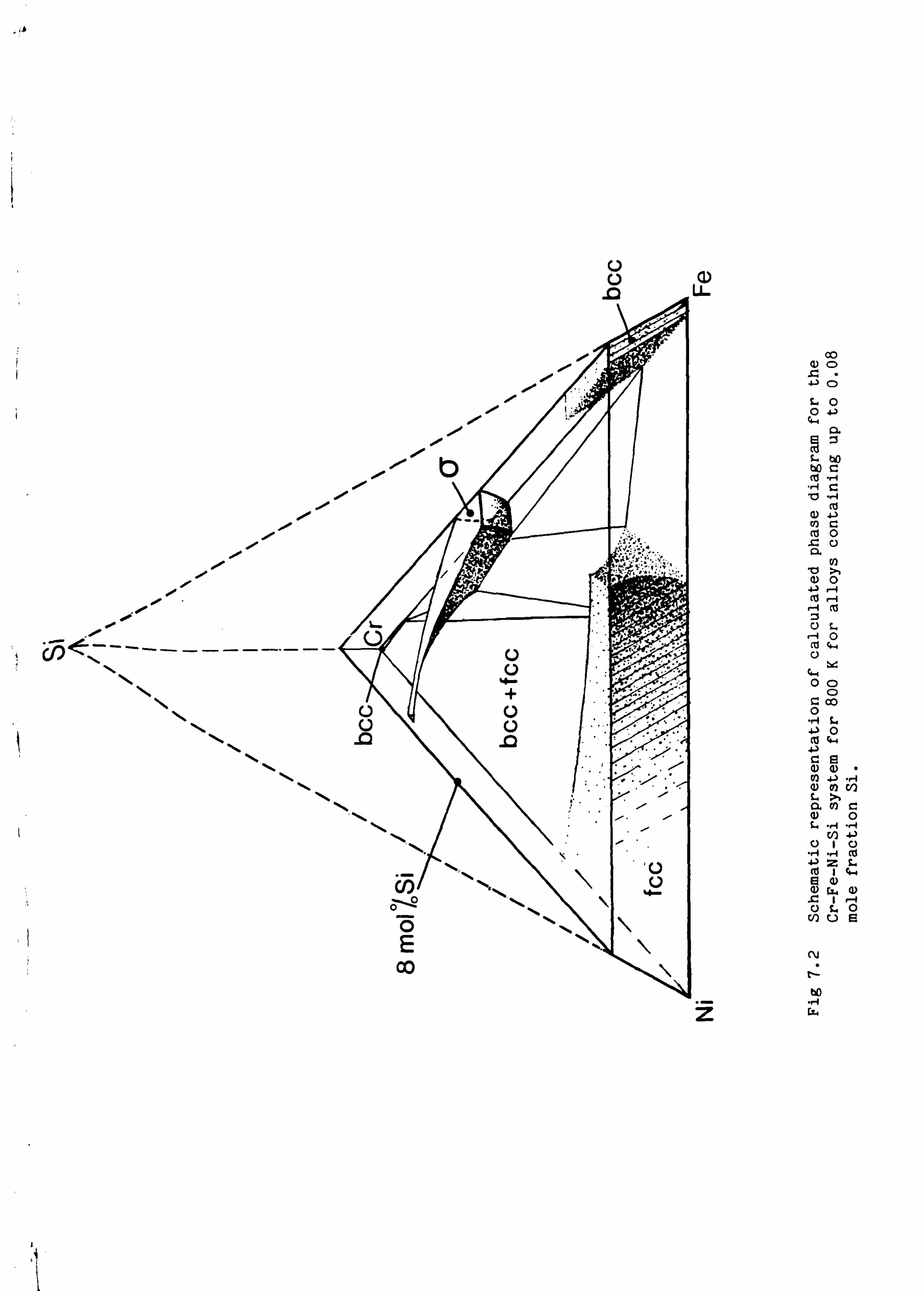
-. 4
i i i i
. ice
IN.
U U n LL
OD ago 4-) 0
LO O4 04
a
L Op eo c "4-+
cKI I V) c cd O .cO a
U) a) O 4.3 1-4 'a-I
as U
O cd 4. U
h4 44 OO
0 C co 0 "-4 L. 4O row ca
a) 4. ) "-4 (L) m CO L. >, amc a) 0
UIU .1 . r1 ft1
2L co I 4"+ aO
L" I rß-1 UO
Cl) O6
N
ýý
Z
ti eo

Fig 7.3 Output from MULTIPHASE for the calculation of the compositions and types of phases in equilibrium for the Cr-Fe-Ni-Si-Ti system at 900 K for a given overall composition.
TEMPERATURE 900.000
COMPONENT QUANTITIES CR 1.400000D-01 FE 7.400000D-01 NI 8.000000D-02 SI 3.00000OD-02 TI 1.000000D-02
SUM OF COMPONENTS = 1.000000D 00 INITIAL POINT SET BY PROGRAM
ERROR IN AMOUNT IS LESS THAN 1.5D-05
PHASE SPECrPHASE AMOUNT(N) MOLE FRACTION -IES PRESENT
STOICHIOMETRIC PHASES CR3SI 1 1 0 CR5S13 2 1 0 FE5SI3 3 1 0 FESI 4 1 0 NI5SI2 5 1 0 N13TI 6 1 0 S13T15 7 1 0 CRFETI 8 1 0
FCC PHASE CR(FCC) 9 1 1 5.379778D-02 FE(FCC) 9 2 1 2.935041D-01 NI(FCC) 9 3 1 6.083208D-02 SI(FCC) 9 4 1 1.421155D-02 TI(FCC) 9 5 1 1.70304OD-03
PHASE TOTAL IS 4.240486D-01
BCC PHASE CR(BCC) 10 1 1 5.359688D-02 FE(BCC) 10 2 1 4.04143OD-01
NI(BCC) 10 3 1 1.515611D-02 SI(BCC) 10 4 1 1.270697D-02 TI(BCC) 10 5 1 8.293910D-03
PHASE TOTAL IS 4.938969D-01
SIGMA PHASE CR(SIGMA) 11 1 1 3.260506D-02 FE(SIGMA) 11 2 1 4.235062D-02 NI(SIGMA) 11 3 1 4.009348D-03 SI(SIGMA) 11 4 1 3.081402D-03 TI(SIGMA) 11 5 1 2.169456D-06
PHASE TOTAL IS 8.20486OD-02
XNI3 PHASE FEN13FCC 12 1 0 N13SIFCC 12 2 0
HEX PHASE CR2TIHEX 13 1 0 FE2TIHEX 13 2 0
CUB PHASE CR2TICUB 14 1 0 FE2TICUB 14 2 0
GIBBS FREE ENERGY = -7.858971D 03
CHEMICAL POTENTIAL
1.268670D-01 -4.102883D 03 6.921474D-01 -1.257559D 03 1.434555D-01 -2.392371D 04 3.351397D-02 -1.211684D 05 4.016144D-03 -8.050750D 04
1.085184D-01 -4.102883D 03 8.182741D-01 -1.257559D 03 3.068679D-02 -2.392371D 04 2.572798D-02 -1.211684D 05 1.679280D-02 -8.050750D 04
3.973872D-01 -4.102883D 03 5.161650D-01 -1.257559D 03 4.886552D-02 -2.392371D 04 3.755581D-02 -1.211684D 05 2.644110D-05 -8.050756D 04
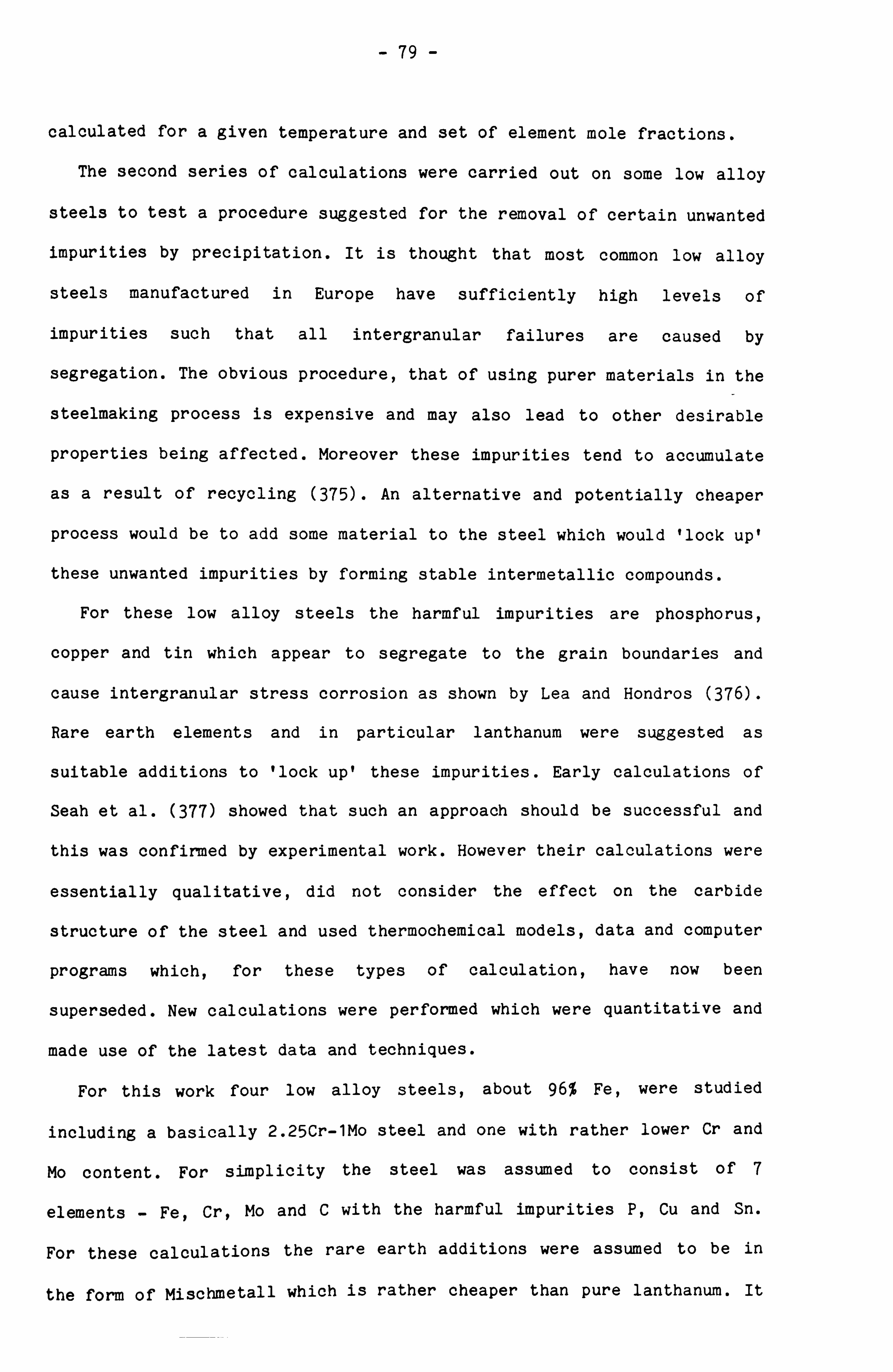
- 79 -
calculated for a given temperature and set of element mole fractions.
The second series of calculations were carried out on some low alloy
steels to test a procedure suggested for the removal of certain unwanted
impurities by precipitation. It is thought that most common low alloy
steels manufactured in Europe have sufficiently high levels of
impurities such that all intergranular failures are caused by
segregation. The obvious procedure, that of using purer materials in the
steelmaking process is expensive and may also lead to other desirable
properties being affected. Moreover these impurities tend to accumulate
as a result of recycling (375). An alternative and potentially cheaper
process would be to add some material to the steel which would 'lock up'
these unwanted impurities by forming stable intermetallic compounds.
For these low alloy steels the harmful impurities are phosphorus,
copper and tin which appear to segregate to the grain boundaries and
cause intergranular stress corrosion as shown by Lea and Hondros (376).
Rare earth elements and in particular lanthanum were suggested as
suitable additions to 'lock up' these impurities. Early calculations of
Seah et al. (377) showed that such an approach should be successful and
this was confirmed by experimental work. However their calculations were
essentially qualitative, did not consider the effect on the carbide
structure of the steel and used thermochemical models, data and computer
programs which, for these types of calculation, have now been
superseded. New calculations were performed which were quantitative and
made use of the latest data and techniques.
For this work four low alloy steels, about 96% Fe, were studied
including a basically 2.25Cr-lMo steel and one with rather lower Cr and
Mo content. For simplicity the steel was assumed to consist of 7
elements - Fe, Cr, Mo and C with the harmful impurities P, Cu and Sn.
For these calculations the rare earth additions were assumed to be in
the form of Mischmetall which is rather cheaper than pure lanthanum. It

- 80 -
was taken to consist of equal proportions of La and Ce. Any oxygen or
sulphur impurities in the steel which had not been removed by manganese,
aluminium or titanium added were predicted to react with the Mischmetall
in preference to the other impurities forming stable oxysulphides (e. g.
La202S). Thermodynamic data were derived or taken from the ALLOYDATA
database for the bcc phase in the 36 component binary systems of the
nine component system and 35 selected stoichiometric binary compounds in
order to calculate the equilibria for certain ranges of composition
between temperatures of 800 K and 1200 K. Cementite, Fe3C, was included
in the calculations in spite of the fact that it is known to be
metastable relative to ferrite and graphite. In practice it is known
that the kinetics favour its formation and that it is stabilised by
small quantities of other elements.
Calculations were performed using Eriksson's SOLGASMIX computer
program (276,277) suitably modified to allow the representation of a
multicomponent bcc solution phase in terms of a Redlich-Kister
polynomial (296). The equilibrium assemblage was calculated for various
additions of Mischmetall to the steels. Fig 7.4 shows the output for a
typical calculation. These calculations represented a considerable
advance over earlier calculations involving the precipitation of
compounds in steels (255,377). In these previous calculations the
interactions between different solute atoms were neglected and no
account was taken of the relative amounts of the minor constituents.
Consequently the calculations could not predict accurately the
distribution of the minor elements between the various competing phases.
The dataset and computer program used for these calculations do not
suffer from such limitations and can in principle be used for a wide
range of compositions and temperatures.
Fig 7.5 and Fig 7.6 show the distribution of C and the harmful
impurities P. Sn and Cu between the bcc phase and the competing

Fig 7.4 Output from SOLGASMIX for of carbon and the harmful various competing phases addition of Mischmetall.
T= 1000.00 K P=1.000E+00 ATM
the calculation of the distribution impurities P, Cu and Sn between the
in a low alloy steel following the
INPUT AMOUNT EQUIL AMOUNT MOLE FRACTION ACTIVITY MOL MOL
FE(BCC) 0.96128E+00 0.96128E+00 0.97808E+00 0.97895E+00 CE(BCC) 0.10000E-02 0.10000E-02 0.10175E-02 0.54417E-07 LA(BCC) 0.10000E-02 0.58880E-07 0.59909E-07 0.92097E-04 CU(BCC) 0.11000E-02 0.64531E-03 0.65659E-03 0.86374E-01 SN(BCC) 0.60000E-04 0.15726E-05 0.16001E-05 0.31136E-05 C(BCC) 0.56000E-02 0.19858E-03 0.20205E-03 0.25936E-07 CR(BCC) 0.23100E-01 0.15778E-01 0.16053E-01 0.88276E-01 P(BCC) 0.22000E-03 0.27904E-09 0.28392E-09 0.18416E-14 MO(BCC) 0.61000E-02 0.39219E-02 0.39905E-02 0.10951E+00
FE17CE2 0.00000E+00 0.00000E+00 0.96204E+00 FE2CE 0.00000E+00 0.00000E+00 0.19278E-01 FE3SN 0.00000E+00 0.00000E+00 0.59943E-01 FE3SN2 0.00000E+00 0.00000E+00 0.10857E-01 FESN 0.00000E+00 0.00000E+00 0.32117E-02 FE3C 0.00000E+00 0.00000E+00 0.60417E+00 FE3P 0.00000E+00 0.00000E+00 0.11421E-01 FE3MO2 0.00000E+00 0.00000E+00 0.51101E+00
CECU 0.00000E+00 0.00000E+00 0.15747E-02 CECU2 0.00000E+00 0.00000E+00 0.40140E-01 CECU4 0.00000E+00 0.00000E+00 0.18689E+00 CECU5 0.00000E+00 0.00000E+00 0.27088E+00 CECU6 0.00000E+00 0.00000E+00 0.33304E+00 CE2SN O. 00000E+00 0.00000E+00 0.68186E-02 CE2SN3 0.00000E+00 0.00000E+00 0.31549E-02 CESN3 0.00000E+00 0.00000E+00 0.12258E-02 CEC2 0.00000E+00 0.00000E+00 0.11762E+00 CEP 0.00000E+00 0.00000E+00 0.23773E-01 LACU 0.00000E+00 0.00000E+00 0.66237E-01 LACU2 0.00000E+00 0.00000E+00 0.48429E+00 LACU5 0.00000E+00 0.00000E+00 0.93737E+00 LACU6 0.00000E+00 0.53056E-03 0.10000E+01 LA2SN 0.00000E+00 0.17546E-03 0.10000E+01 LA2SN3 0.00000E+00 0.00000E+00 0.62822E-01 LASN3 0.00000E+00 0.00000E+00 0.79501E-02 LAC2 0.00000E+00 0.17629E-02 0.10000E+01 LAP 0.00000E+00 0.44000E-03 0.10000E+01 CU31SN8 0.00000E+00 0.00000E+00 0.31464E-01 CU3SN 0.00000E+00 0.00000E+00 0.20246E-01 CUSP 0.00000E+00 0.00000E+00 0.27312E-02 CUP2 0.00000E+00 0.00000E+00 0.11524E-07 C2CR3 0.00000E+00 0.00000E+00 0.98823E+00 C3CR7 0.00000E+00 0.10461E-01 0.10000E+01 C6CR23 0.00000E+00 O. 00000E+00 0.52446E+00 CM02 0.00000E+00 0.32654E-02 0.10000E+01
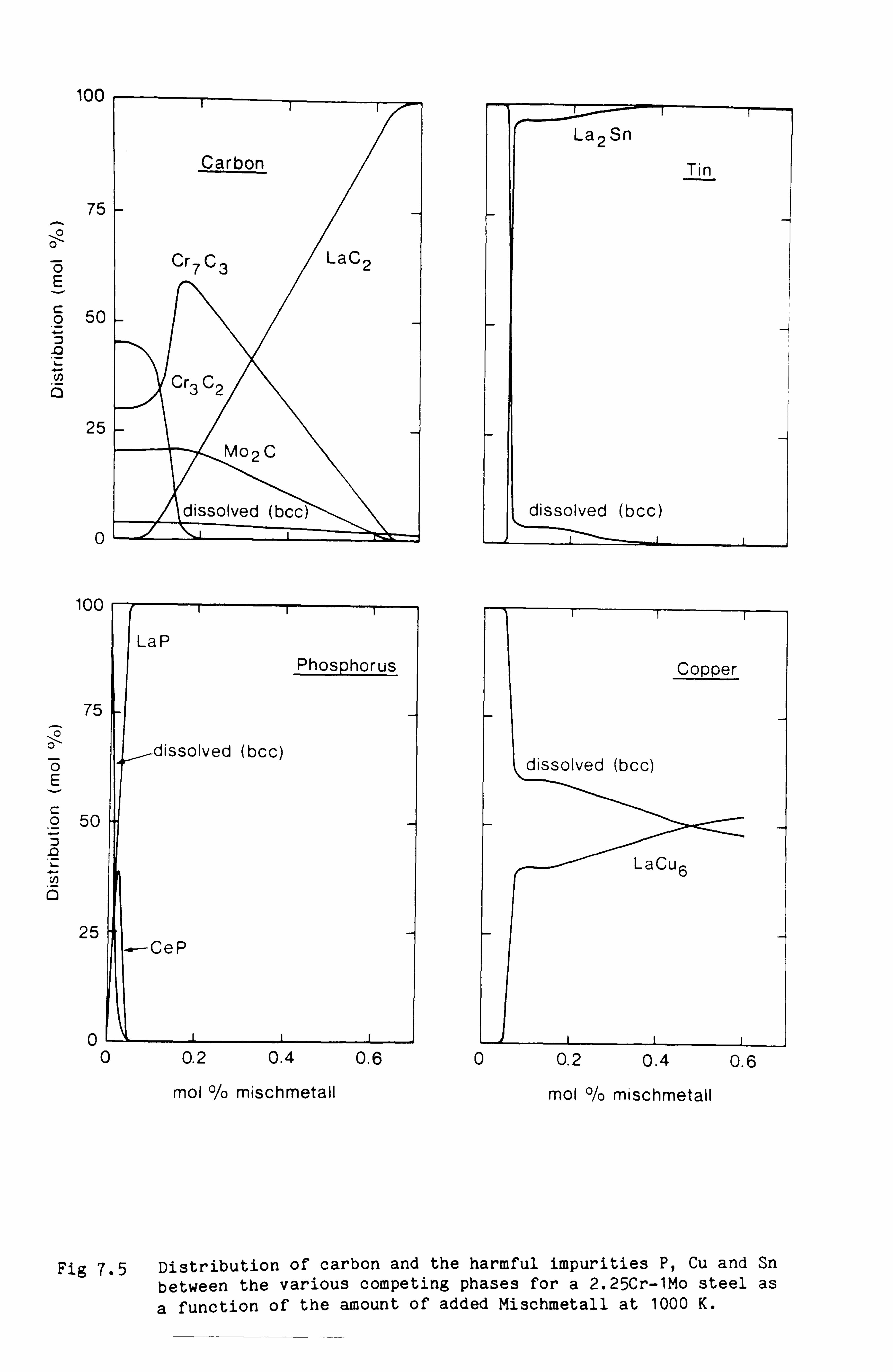
100
75 0- 0 Ö E
ö 50
ö
25
0
100
Carbon
Cr7C3 LaC2
Cr3 C2
MoeC
dissolved (bcc)
II LaP Phosphorus
75
0
O
c 0 50
D
C,,
a
25
oý 0
issolved (bcc)
La2Sn
Tin
dissolved (bcc)
Copper
dissolved (bcc)
LaCu6
CeP
0.2 0.4 0.6
mol % mischmetall
0 0.2 0.4 0.6
mol % mischmetall
Fig 7.5 Distribution of carbon and the harmful impurities P, Cu and Sn between the various competing phases for a 2.25Cr-1Mo steel as a function of the amount of added Mischmetall at 1000 K.
100
Carbon
75
Ö E
ö 50
ö
25
0
LaC2
Fe 3C
dissolved (bcc)
Cr3C2
Mo2C
100
75
O E
C
0 50 :r
cn 0
LaP
25
Phosphorus
dissolved (bcc)
CeP
oý 0 0.2 0.4 0.6
mol % mischmetall
1 dissolved (bcc)
Tin
La2Sn
Copper N
dissolved (bcc)
LaCu6
0 0.2 0.4 0.6
mol % mischmetall
Fig 7.6 Distribution of carbon and the harmful impurities P, Cu and Sn
between the various competing phases for a low alloy steel as
a function of the amount of added Mischmetall at 1000 K.

- 81 -
intermetallic compounds for two of the steels under study at 1000 K. It
can be seen from these calculations that lanthanum is a far more
effective additive than cerium. Fig 7.5, for a 2.25Cr-lMo steel shows
that relatively small amounts of Mischmetall need be added in order to
obtain essentially complete removal of phosphorus and tin as LaP and
La2Sn respectively and removal of 40% of Cu in the form of LaCu6. It
should be mentioned that this work predicts the removal of phosphorus
before tin in contrast to that predicted by Seah et al. (377) . This is
due largely to the more reliable thermodynamic data available now. The
removal of phosphorus is most important since phosphorus is known to be
very embrittling in a 2.25Cr-Mo steel. Seah et al. were unable to gauge
the effect of the addition of the Mischmetall on the carbide structure
of the steel. Fig 7.5 shows this to be unaffected for relatively modest
additions of Mischmetall.
Fig 7.6, on the other hand, which represents the effect of
Mischmetall on a steel with rather less Cr and Mo, shows that while
relatively small amounts of Mischmetall are required to remove
phosphorus, large amounts are required to have any effect on the levels
of dissolved tin and copper. By that stage the Mischmetall additions
would have affected the carbide structure of the steel to the extent
that its physical properties would no longer be within the
specification.
The difference between the two steels can be attributed to the lower
Cr and Mo content in the steel represented by Fig 7.6. For the
2.25Cr-lMo steel (Fig 7.5) the activity of carbon in the bcc phase is
effectively lowered by the formation of the stable carbides Cr3C2, Cr7C3
and Mo2C. This allows Mischmetall to react with the tramp elements. For
Fig 7.6 the carbon activity is higher promoting reaction with the
Mischmetall before the Mischmetall can react with the tin or copper.
This work was able to define successfully a range of Mischmetall

- 82 -
additions to various steels to provide, in theory, immunity to stress
corrosion cracking. The results are based on thermodynamic data and do
not take into account the kinetics of phase transformation which can
also be expected to be important. However the results can be applied
with confidence when predicting the long term stability of materials.
Conclusions
Presented in this chapter is a brief description of two sets of
calculations from thermodynamic data which have been performed to
elucidate the long term stability of certain steels. The work has
utilised the latest techniques for the calculation of phase equilibria
and representation of thermodynamic data. More calculations of
importance to industry can be performed readily, especially when the
thermodynamic database has been expanded to cover more elements.

- 83 -
CHAPTER 8
Phase Diagrams and Thermodynamic data for Cu-Fe-Ni-S system
Introduction
The aim of this work was to gain greater understanding of the phase
equilibria in the metal rich part of the Cu-Fe-Ni-S system in order to
help improve the pyrometallurgical extraction of copper and other
valuable metals from sulphide ores based on this system. Experience has
shown that phase transformations in these systems occur readily at
moderate temperatures and this suggests that a reliable way for
understanding and predicting behaviour would be to perform calculations
of the phase diagram from the thermodynamic data. The success achieved
for alloy systems in the calculation of multicomponent thermodynamic
data and phase diagrams from the thermodynamic data of the component
binary systems has led to the adoption of this approach for sulphide
systems.
Representation of Data for the Liquid Phase
The major problem associated with this work was the representation of
the thermodynamic data in terms of composition for the different phases.
The liquid phase is particularly difficult to represent because in all
metal-sulphur systems its thermodynamic properties show marked changes
at particular compositions. These compositions differ from system to
system and it has been proposed that this phenomenon was due to some
sort of ordering. Conventional power series expressions such as the
Redlich-Kister expression are not capable of representing the data
adequately although Pelton and Bale (161) have represented the liquid

- 84 -
data for the Cu-Fe-S system using a Fourier cosine series. Clearly any
reliable method for predicting multicomponent phase diagrams must
attempt to model this physical ordering phenomenon.
As discussed in chapter 3 much research has already been carried out
into methods for representing the data for these sulphide liquids. In
particular it is worth emphasising the work of Kellogg, Larrain and
their colleagues (213,214,217,219,220,378-382) who have carried out
extensive measurements of sulphur pressures above the liquid phase and
modelled their data in terms of associated species. Their work should
not, however, be thought of as predictive but rather as a correlation of
the data in terms of a large number of coefficients and associate
species. Chang and his colleagues (74,204,216,221,223,383,384) have also
been interested in these systems and have also used the associated
solution model for the liquid phase. Their approach has been rather more
predictive and they have attempted to represent both liquid and solid
phases with as few coefficients as necessary.
The other major effort on these systems to date was from Hillert and
his colleagues (229,231-233) who have advocated the use of an extended
two sublattice model for the liquid phase whereby metal atoms and
vacancies mix on the first sublattice and sulphur atoms and vacancies
mix on the other sublattice. Except for their treatment of the metal
rich part of the Fe-Mn-S system (231) using a simplified description
they have not reported any ternary sulphide phase diagram calculations.
An extensive analysis of the different models on the Fe-S and Cu-S
system was carried out in this present work leading to the conclusion
that an extended two sublattice model was best suited to represent the
complex behaviour of these systems. This model was chosen because it
seems in principle physically more realistic than the associated
solution model for melts of substances that as crystals have extended
rather than molecular bonding such as mattes. Because of this it should

- 85 -
offer superior prospects for the extrapolation of the binary
thermodynamic data for the liquid phase into the ternary and quaternary
systems without the necessity of introducing an excessive number of
ternary or higher order parameters. This extrapolation is vital for the
correct prediction of the phase diagram for the Fe-Cu-Ni-S system.
For the Fe-S liquid phase Fernandez Guillermet et al (232-233)
assumed that there was an equal number of sites in the two sublattices
which reflects the abrupt change in the thermodynamic properties at
about the composition xS-0.5. For the Cu-S system this abrupt change in
behaviour occurs at about xS=0.33 while in the Ni-S system it occurs at
about xS=0.4. A number of variations of the two sublattice model could
in principle be used to represent the liquid data of the Cu-S system.
However, it is important that the model, in addition to representing the
Cu-S binary data accurately and extrapolating them reliably into a
ternary system, is consistent with accepted descriptions for the other
component systems.
One model that was tested allows the combination of the data for the
Fe-S system (1: 1 site ratio) with data for the Cu-S system derived
assuming a 2: 1 ratio of the number of sites between the sublattices.
This ratio of sites for the Cu-S system is implied by the change in the
thermodynamic properties at about xs=0.33. It assumes that in the
ternary system the copper atoms can occupy twice as many sites as the
iron atoms even though the iron and copper atoms would mix together on
the same sublattice. In effect an iron atom would occupy twice the space
occupied by a copper atom. Even though trial calculations made with this
model were in good agreement with available experimental data it
required a non-conventional and non-physical representation of the
thermodynamic data for the copper-iron binary system.
A second model, based on a suggestion of Hillert (385), does not
suffer from such a drawback. It assumes that the liquid phase consists
- 86 -
of ions and charged vacancies. Vacancies would be considered as having a
charge equal in magnitude but opposite in sign to a corresponding ion on
the other sublattice. Hillert proposed that copper would be univalent
while iron and sulphur would be divalent. Therefore for the Cu-S liquid
phase, on the metal sublattice there would be copper ions and vacancies
with a charge of +2 while on the sulphur sublattice there would be
sulphur ions and vacancies with a charge of -1. The ratio of sites
between the two sublattices would not be fixed but would be defined by a
charge balance between the various ions and charged vacancies. There is
however no suggestion that these charges are formally present.
According to the original approach suggested by Hillert, the ternary
Cu-Fe-S liquid phase could be represented in terms of two sublattices
with three species on each sublattice. The metal sublattice would
consist of Fe+2 and Cu+ ions and vacancies with a +2 charge. The sulphur
sublattice would consist of S-2 ions with two types of vacancy to
balance the two types of metal ions on the other sublattice. This has a
severe disadvantage in requiring many data that are unavailable from the
component binary systems. The model was therefore modified so as to
require only one type of vacancy on the sulphur sublattice where its
charge would be non-integral varying according to the relative amounts
of copper and iron in the phase.
This model was also tested for its capability for extrapolation into
the Cu-Fe-S system and was found to give excellent agreement with the
ternary experimental data. This together with its use of conventionally
represented Cu-Fe data led to the adoption of this model to represent
the liquid phase thermodynamic data for phase diagram calculations.
The general multicomponent model for metal-sulphides will now be
described and an expression derived for the Gibbs energy of formation of
compositions in that phase.

- 87 -
Details of liquid phase model
First of all we can consider that the phase contains m elements - ie.
m-1 metallic elements plus sulphur. The metal atoms in the system can be
designated by Ai and their the mole fractions by xi while the mole
fraction of sulphur will be xs.
In the two sublattice model adopted for this work it is assumed that
the metal atoms and sulphur atoms occupy different sublattices.
Following Hillert's suggestion (385) each species in the phase carries a
notional charge. We can define the charge of the sulphur species as -b
and the charge on each metal atom as +ai. Vacancies are included in each
of the sublattices and they also have charges. In the case of the
vacancies Va on the metal sublattice the charge will be opposite in sign
but equal in magnitude to the charge on the sulphur atoms in the second
sublattice ie. +b. The charge -e on the vacancies Vc in the second
sublattice would vary according to the relative proportions of metal
ions and their charges according to:
ID-1 5a. xi i=1 1 e
m-1 ýx. i=1 1
For convenience we can designate the phase in terms of the various
species on the two sublattices as:
C Miai9....., Va+b ][ S-b, Vc-e ]q P
where p and q are the number of sites on the two sublattices per unit
cell. It is often convenient to choose the value of q as 1. The ratio of
p to q is not fixed for the whole phase but is defined by a condition
that the system should be electrically neutral.

- 88 -
It is useful to define a variable s, the size of the system given by:
M-1 xi + XVa x+ XVc
S= i=1 = Pq
2
For simplicity it is also useful to designate xVa as xm. For each
species it is necessary to define a site fraction Z1 such that:
Xi
z. 1 m
X
k=1 k
3
where in this case the species i is on the first sublattice. The site
fractions of species on the second sublattice can be defined in a
similar way.
Since the phase is electrically neutral it is possible to derive a
relationship between p and q.
M-1 57 a1xi +b xVa =b xs +e xVe i=1
According to equation 2
: 11 + XVa =Ps
and
xs + xvc =qs
Substituting these into the above equation and rearranging one obtains:
M-1 m-1 m-1 m-1 x1 ai xi +bps Xi -b (I Xi)2 =
i=1 i=1 i=1 i=1
M-1 m-1 m-1 b xs xi +qs aixi - xS : aixi
1=1 i=1 i=1
which gives, on further rearrangement and through application of the
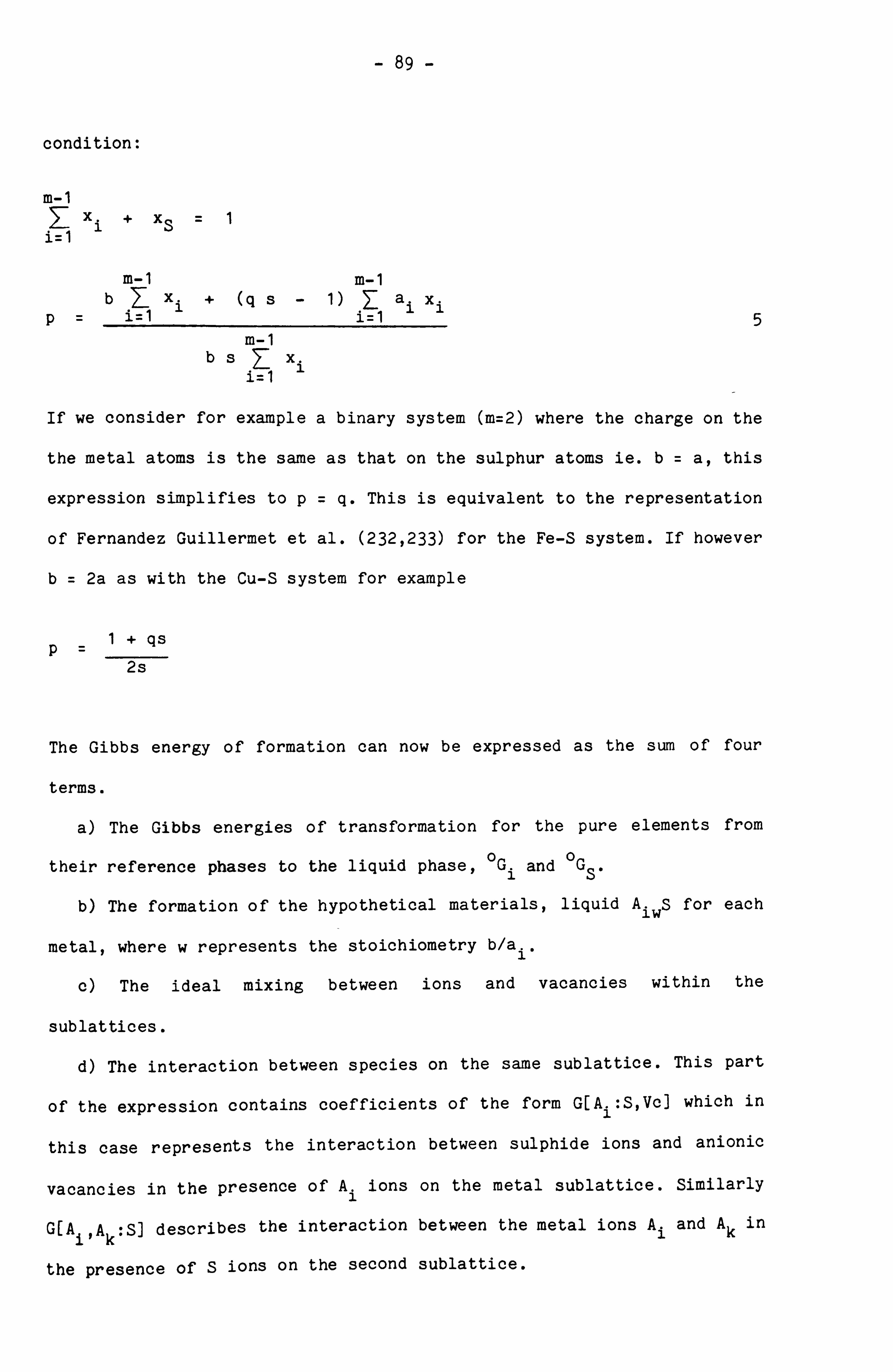
- 89 -
condition:
M-1 xi + xS
i=1
M-1 m-1 b xi + (q s- 1) 37 ai xi
P= i=1 i=1 5 M-1
bs 7- xi i=1
If we consider for example a binary system (m=2) where the charge on the
the metal atoms is the same as that on the sulphur atoms ie. b=a, this
expression simplifies to p=q. This is equivalent to the representation
of Fernandez Guillermet et al. (232,233) for the Fe-S system. If however
b= 2a as with the Cu-S system for example
p+ qs 2s
The Gibbs energy of formation can now be expressed as the sum of four
terms.
a) The Gibbs energies of transformation for the pure elements from
their reference phases to the liquid phase, 0Gi and 0 GS.
b) The formation of the hypothetical materials, liquid AiWS for each
metal, where w represents the stoichiometry b/ai,
c) The ideal mixing between ions and vacancies within the
sublattices.
d) The interaction between species on the same sublattice. This part
of the expression contains coefficients of the form G[Ai: S, Vc] which in
this case represents the interaction between sulphide ions and anionic
vacancies in the presence of A1 ions on the metal sublattice. Similarly
G[Aj, Ak: S] describes the interaction between the metal ions Ai and Ak in
the presence of S ions on the second sublattice.

- 90 -
The Gibbs energy of formation is therefore given by:
m-1
fG => Xi 0 Gi + xs °Gs
i=1
m-1 +s{ ZiZS °GA
S i=1 w i
m
+RTp[ Ziln Zi] i=1
+RTq[ ZS In ZS + ZVc In ZVc
mr +E ZiZSZVc ö G[Ai: S, Vc]h (ZS - ZVc)h
m-1 mr + ZS Y 7- Zi Zk 7 G[Al, Ak: S]h (Zi - Zk)h
i=1 k=i+1 h=0
m-1 mr + ZVc Zi Zk I G[Ai, Ak: Vc]h (Zi - Zk)
h
i=1 k=i+1 h=0
m-2 m-1 rt + ZSZVc Zi Zk 1Z G[Ai, Ak: S, Vc]h 1 i=1 k=i+1 h=0 1=0 '
(Zi - Zk)h (ZS -z VC) 1}
t
where, for example, h defines the coefficient of the polynomial up to
the maximum order r.
The Gibbs energy of formation is a function of the size of the system
s which is related to the total population of the vacancies within the
phase. This is not defined directly by the model and it is necessary to
find the value of s which will give the lowest value for the Gibbs
energy of formation. This will in turn describe the vacancy population.
It is not possible to solve this problem explicitly and it is
neccessary to use some sort of numerical technique to determine the
conditions for the minimum value of the Gibbs energy. A convenient

- 91 -
method is to use a Newton-Raphson method whereby one searches for the
values of s that satisfies the condition that (dG/ds)=0. An explicit
expression was derived for this first differential while the second
differential (d2G/ds2) was evaluated numerically from the first
differential evaluated for two very close values of s. For a given
estimate of s the first and second derivatives can be combined to lead
to a better value which can itself be used in the same way and so_ on
until the required accuracy has been obtained.
The differential of the Gibbs energy of formation with respect to the
size of the system is given by:
M-1 d ýfG =-k ZS I Zi oGA
A. S ds 1=1 1w
+RTpk 1n(ZVa) +RTq 1n(ZVc)
m-1 r + ZS(ZS -k ZVo) 1 Zi E G[Ai: S, Vc]h (ZS - ZVc)h
i=1 h=0
r + ZS(k ZVc(1 - ZVa) + ZVaZVc) Z G[Va: S, Vc]h (Z
s- ZVc)h
h=0
- 2Z2Z 'Z Zi Lh G[Ai: S, Vc]h (ZS - ZV0)h-1 S Vc i=1 h=1
m-2 m-1 r -2k ZS 7 Zi E Zk > GLAI, Ak: S]h (Z1 - Zk
i
)h
=1 k=1 h=0
m-1 r +k ZS (1 -2 ZVa) E Zi L G[Al, Va: S]h (Zi - ZVa)h
i=1 h=0
m-2 m-1 r
-kZ7 Zi Zk (Zi - Zk) h GLAi, Ak: S]h (Zi - Zk)h-1 S i=1 k=i+1 h=1
m-2 m-1 r + (1 -2k VC) 1 Zi Zk : G[Al, Ak: Vc]h (Zi - Zk)h
i=1 k=i+1 h=0
m-1 r
+ (Z + ZVc k (1 -2 ZVa) Z Zi Z G[Ai, Va: Vc]h (Zi- ZVc)h Va i=1 h=0

- 92 -
m-2 m-1 -kZ Vc
7 7-
i=1 k=i+1 Zi Zk (Zi-Zk)
r 2h G[Ai, Ak: Vc]h (Zi-Zk)h-1
h=1
M-1 r -k ZVc ZVa Zi (1+Zi-ZVa) Zh G{Ai, Va: Vc]h (Zi-ZVc)h-1
i=1 h=1
m-1 -k ZS ZVa I Zi (1 + Zi - ZVa)
i=1
m-2 m-1 + ZS (ZS -2k ZVc) F Zi 7
i=1 k=i+1
r Lh G[Ai, Va: S]h (Zi-ZVc)h-1
h=1
rt Zk GCAi, Ak: S, Vc]h
' s h=0 1=0
(Zi - Zk) h (Zs - Zve)1
m-2 m-1 r t -kZZ S Vc
7- Z Zk ) 1kk
h G[A1. 'Ak: S Vc]h l i=1 k=i+1 h=1 1=0 ,
(Z1 - Zk)h-1 (z s- ZVe)1
m-2 m-1 rt -2 ZS ZVe Y3 Zi Zk >L1 GCAi, Ak: S, Vc3h'1
i=1 k=i+1 h=0 1=1
(Z1 - Zk) h (Zs - Zvc)1-1
where k=Qe bp

- 93 -
Representation of data for the other phases
The thermodynamic data for the bcc, fcc and L12 phases of the
metal-metal binary systems were represented by the widely used Redlich -
Kister power series for the excess Gibbs energy of formation. It was
assumed that the solubility of sulphur in these phases could be
neglected. Using the binary data for the metallic systems which were
combined using the Redlich-Kister ternary expression, Chart et al. (169)
calculated the phase diagram for the Cu-Fe-Ni system over a range of
temperatures and obtained good agreement with available experimental
information. These data were therefore used for the Cu-Fe-Ni-S system.
Therefore for these phases containing m elements Ai where xi denote
their mole fractions, the Gibbs energy of formation from chosen
reference phases for the pure elements is given by:
LG_ xi °Gi
i=1
m +RT xi ln(xi)
i=1
m-1 mr +y xixj E
i=1 j=i+1 h=0
m-2 m-1 m + ý
i =1 j=i+1 k=j 1
G[Ai, Aj]h (xi-xj) h
xlxjxk G[Ai, Aj, Ak]
where °G represents the Gibbs energies of transformation for the pure
element i from its reference phase at the temperature T, G[Ai, Aj]h
represents the h'th order coefficient for the binary interactions
between atoms of A. and atoms of Aj, G[Ai, Aj, Ak] represents the ternary
interaction between elements A1, A and Ak and R represents the gas
constant. All of the terms 0 Gi, G[Ai, Aj]h and G[Ai, Aj, Ak] can be
expressed as a function of temperature.
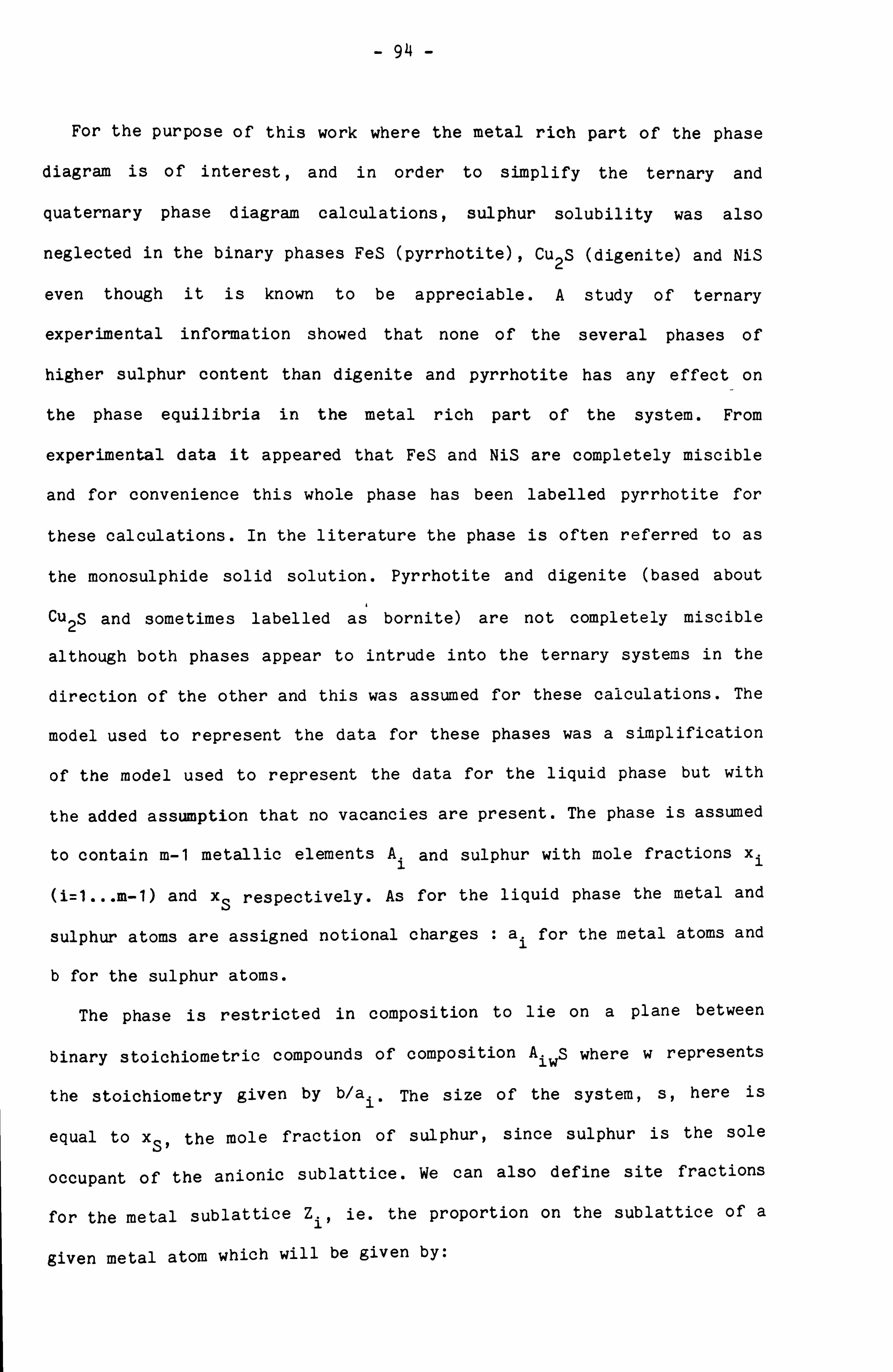
- 94 -
For the purpose of this work where the metal rich part of the phase
diagram is of interest, and in order to simplify the ternary and
quaternary phase diagram calculations, sulphur solubility was also
neglected in the binary phases FeS (pyrrhotite), Cu2S (digenite) and NiS
even though it is known to be appreciable. A study of ternary
experimental information showed that none of the several phases of
higher sulphur content than digenite and pyrrhotite has any effect on
the phase equilibria in the metal rich part of the system. From
experimental data it appeared that FeS and NiS are completely miscible
and for convenience this whole phase has been labelled pyrrhotite for
these calculations. In the literature the phase is often referred to as
the monosulphide solid solution. Pyrrhotite and digenite (based about
Cu2S and sometimes labelled as bornite) are not completely miscible
although both phases appear to intrude into the ternary systems in the
direction of the other and this was assumed for these calculations. The
model used to represent the data for these phases was a simplification
of the model used to represent the data for the liquid phase but with
the added assumption that no vacancies are present. The phase is assumed
to contain m-1 metallic elements Ai and sulphur with mole fractions xi
(i=1... m-1) and xs respectively. As for the liquid phase the metal and
sulphur atoms are assigned notional charges : ai for the metal atoms and
b for the sulphur atoms.
The phase is restricted in composition to lie on a plane between
binary stoichiometric compounds of composition AS where w represents
the stoichiometry given by b/ai, The size of the system, s, here is
equal to xSP the mole fraction of sulphur, since sulphur is the sole
occupant of the anionic sublattice. We can also define site fractions
for the metal sublattice Zi, ie. the proportion on the sublattice of a
given metal atom which will be given by:
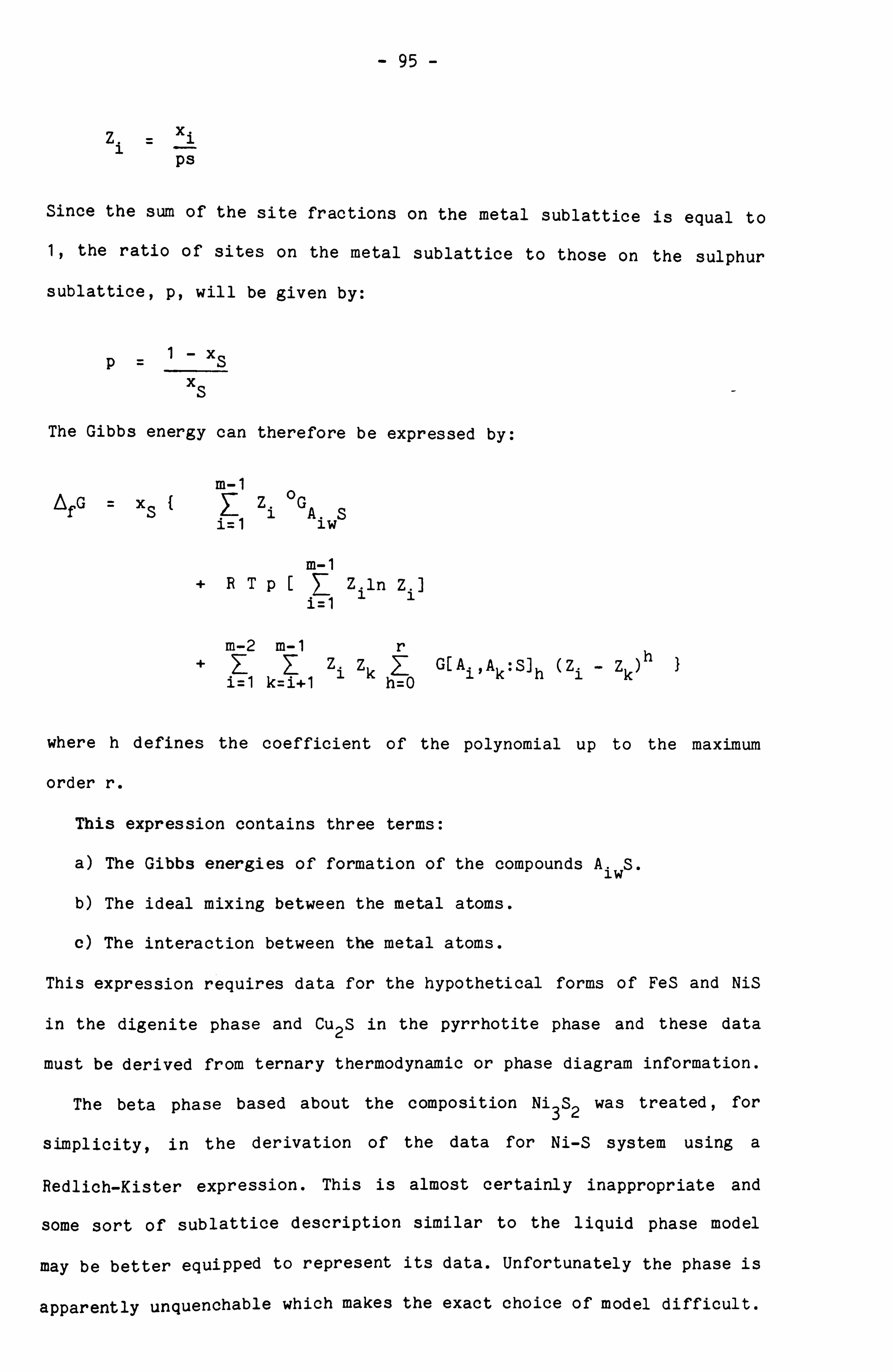
- 95 -
Z. Xi 1- PS
Since the sum of the site fractions on the metal sublattice is equal to
1, the ratio of sites on the metal sublattice to those on the sulphur
sublattice, p, will be given by:
xS
xs
The Gibbs energy can therefore be expressed by:
M-1 Ofd XS { Z. EGA
S i=1 iw
m-1 +RTp[ Zi1n Zi]
i=1
m-2 m-1 r +FE Zi Zk 7
i=1 k=i+1 h=0 G[Ai, Ak: S]h (Zi - Zk) h}
where h defines the coefficient of the polynomial up to the maximum
order r.
This expression contains three terms:
a) The Gibbs energies of formation of the compounds AiWS.
b) The ideal mixing between the metal atoms.
c) The interaction between the metal atoms.
This expression requires data for the hypothetical forms of FeS and NiS
in the digenite phase and Cu2S in the pyrrhotite phase and these data
must be derived from ternary thermodynamic or phase diagram information.
The beta phase based about the composition Ni3S2 was treated, for
simplicity, in the derivation of the data for Ni-S system using a
Redlich-Kister expression. This is almost certainly inappropriate and
some sort of sublattice description similar to the liquid phase model
may be better equipped to represent its data. Unfortunately the phase is
apparently unquenchable which makes the exact choice of model difficult.

- 96 -
Furthermore certain evidence (383,386) suggests that in the Ni-S binary
system the phase region consists of two distinct phases separated by a
narrow two phase region. Both Fe and Cu are appreciably soluble in this
phase and because of the obvious difficulties concerning this phase it
was decided to continue to use, for simplicity, the Redlich-Kister
expression which can be readily extrapolated into a multicomponent
system. The expression for this model-was also used for the bec, fcc and
L12 phase and was shown earlier.
The remaining solution phase of interest in the metal rich part of
the Cu-Fe-Ni-S system is the pentlandite phase (Fe, Ni)9S8. It is
believed that the solubility of Cu and S in this phase is small and was
therefore neglected. This phase was modelled as a conventional
substitutional solution between the Fe and Ni atoms on the metal
sublattice with a second sublattice occupied solely by sulphur atoms.
The ratio of sites between the sublattices is 9: 8.
The remaining phases of interest in this system are the low
temperature binary stoichiometric phases Chalcocite (Cu2S), Millerite
(NiS), Heazlewoodite (Ni3S2) and Ni7S6.
Assessment or Validation of data for the Binary Systems
The Cu-Fe system
The data for this system have been validated by Chart et al. (169). The
phase diagram (Figure 8.1) is well established (44,53,55,387-391)
although the Fe-based fcc solvus reported in earlier compilations, (e. g.
Ref 53) has now been revised (44,387,390). The adopted thermodynamic
data were taken from the assessment of Kubaschewski et al. (390). Other
detailed thermodynamic assessments for this system have been carried out
by Hasebe and Nishizawa (387,388) and Lindqvist and Uhrenius (389).
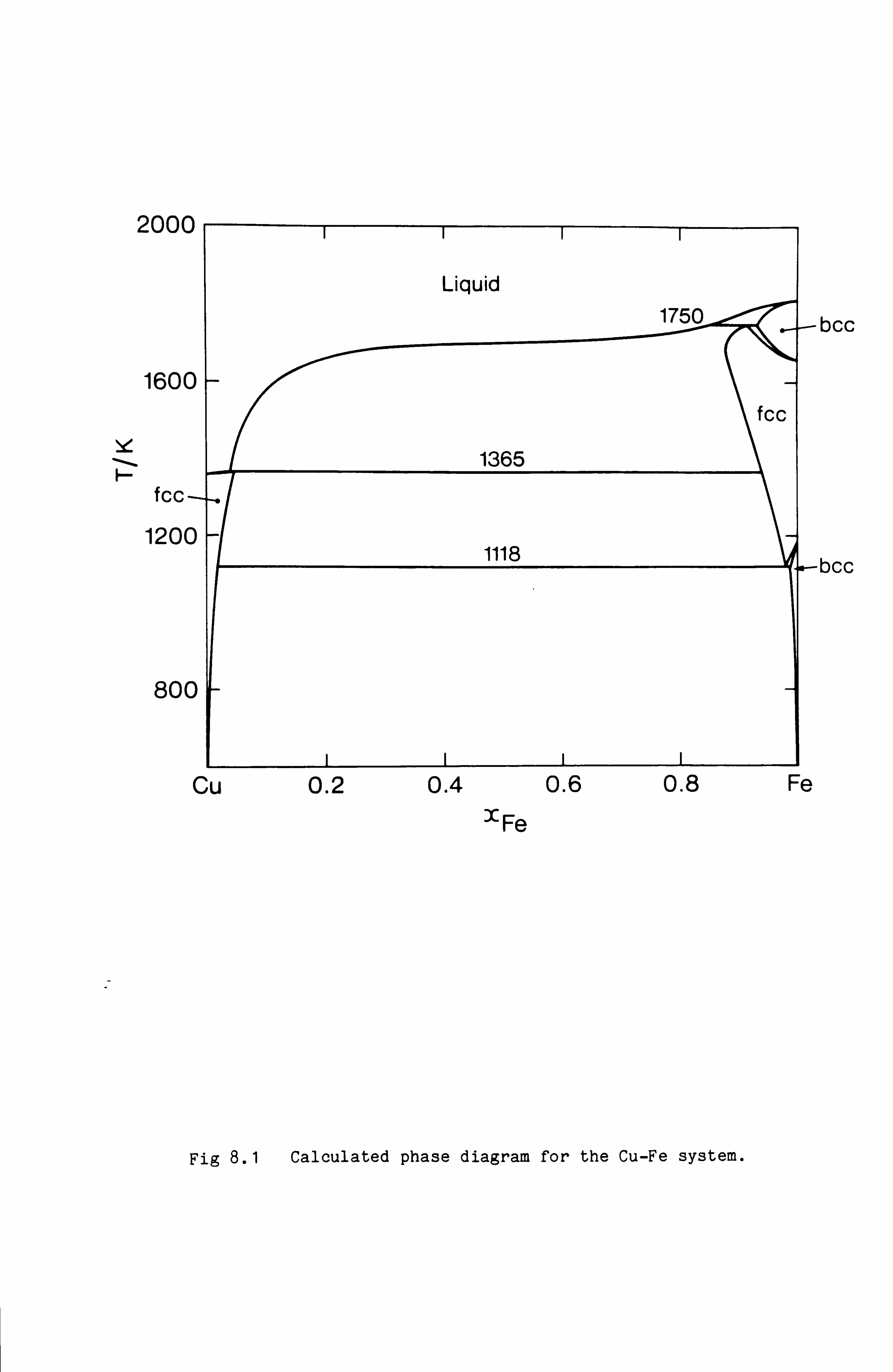
2000
bcc
160(
fcc
120( bcc
801
x Fe
Fig 8.1 Calculated phase diagram for the Cu-Fe system.
Cu 0.2 0.4 0.6 0.8 Fe
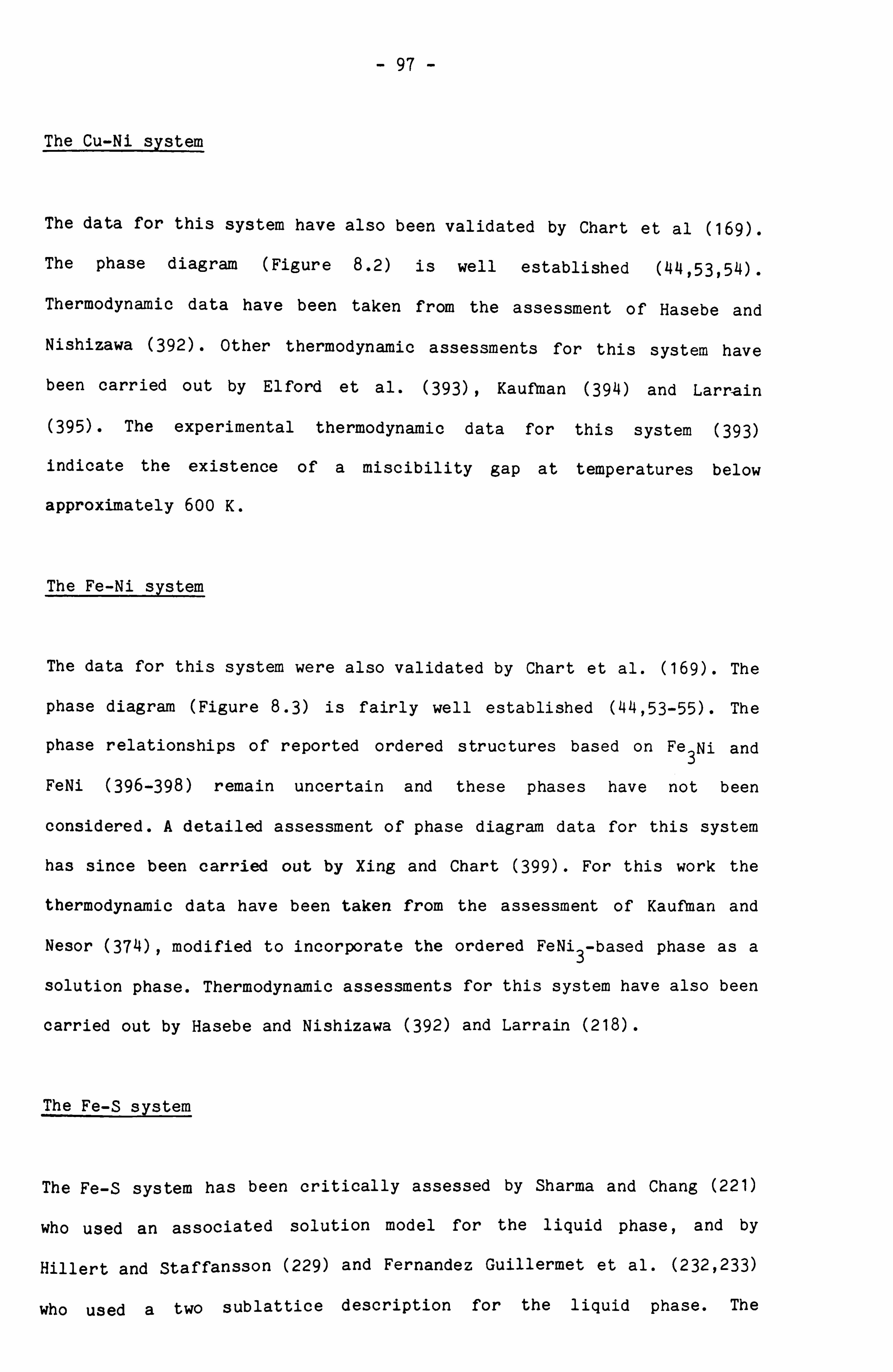
- 97 -
The Cu-Ni system
The data for this system have also been validated by Chart et al (169).
The phase diagram (Figure 8.2) is well established (44,53,54).
Thermodynamic data have been taken from the assessment of Hasebe and
Nishizawa (392). Other thermodynamic assessments for this system have
been carried out by Elford et al. (393), Kaufman (394) and Larrain
(395). The experimental thermodynamic data for this system (393)
indicate the existence of a miscibility gap at temperatures below
approximately 600 K.
The Fe-Ni system
The data for this system were also validated by Chart et al. (169). The
phase diagram (Figure 8.3) is fairly well established (44,53-55). The
phase relationships of reported ordered structures based on Fe3Ni and
FeNi (396-398) remain uncertain and these phases have not been
considered. A detailed assessment of phase diagram data for this system
has since been carried out by Xing and Chart (399). For this work the
thermodynamic data have been taken from the assessment of Kaufman and
Nesor (374), modified to incorporate the ordered FeNi3-based phase as a
solution phase. Thermodynamic assessments for this system have also been
carried out by Hasebe and Nishizawa (392) and Larrain (218).
The Fe-S system
The Fe-S system has been critically assessed by Sharma and Chang (221)
who used an associated solution model for the liquid phase, and by
Hillert and Staffansson (229) and Fernandez Guillermet et al. (232,233)
who used a two sublattice description for the liquid phase. The

2000
Liquid
1600
. 1200 fcc
800
fcc + fcc
400 L Cu 0.2 0.4 0.6 0.8 Ni
XNi
Fig 8.2 Calculated phase diagram for the Cu-Ni system.

2000
Liquid
bcc
1500
Y
1000
bcc
500 u Fe 0.2
fcc
- or L12
0.4 0.6 0.8 xNi
Ni
Fig 8.3 Calculated phase diagram for the Fe-Ni system.

- 98 -
assessment of Fernandez Guillermet et al, is fully compatible with the
liquid phase model described earlier and was therefore adopted for this
present work. The phase diagram calculated using their data is shown in
Figure 8.4 and is in very good agreement with that determined
experimentally. In the original description the pyrrhotite phase was
described as a solution phase. For the reasons described earlier, for
this work it was treated as a stoichiometric phase. In the same way the
solubility of sulphur in solid iron which is very small has been
neglected. The phase diagram calculated using these simplified data is
shown in Figure 8.5. The differences from Figure 8.4 are very slight.
The Cu-S system
The selected phase diagram for the Cu-S system is shown in Fig 8.6. The
diagram has been based primarily on those given in the reviews by Bale
and Toguri (400), Barton (401), Craig and Scott (402), Kellogg (63,213)
and Sharma and Chang (204) but incorporating additional information
(53-55,403-410).
The basic features shown by this diagram are typical of a number of
high affinity systems. The solubility of the solid elements in one
another is very low, there is a compound digenite Cut-xS which melts
congruently and also exhibits non-stoichiometry to sulphur rich
compositions. The liquid phase shows a pronounced tendency to
immiscibility on either side of the composition corresponding to
digenite and sharp changes in the thermodynamic data at about this
composition. These data imply ordering of the liquid phase as confirmed
by electrical conductivity measurements.
Experimental measurements in the Cu-S system are difficult especially
at high sulphur concentrations where the vapour pressure of sulphur can
become very high. On the copper rich side of the diagram the phase

i
F-
2000
1600
1200
800
bcc
bý L2_--
fcc
bcc FeS
FeS2
Fe 0.2 0.4 0.6 0.8 S XS
Fig 8.4 Phase diagram for the Fe-S system calculated using data derived by Fernandez Guillermet et al.
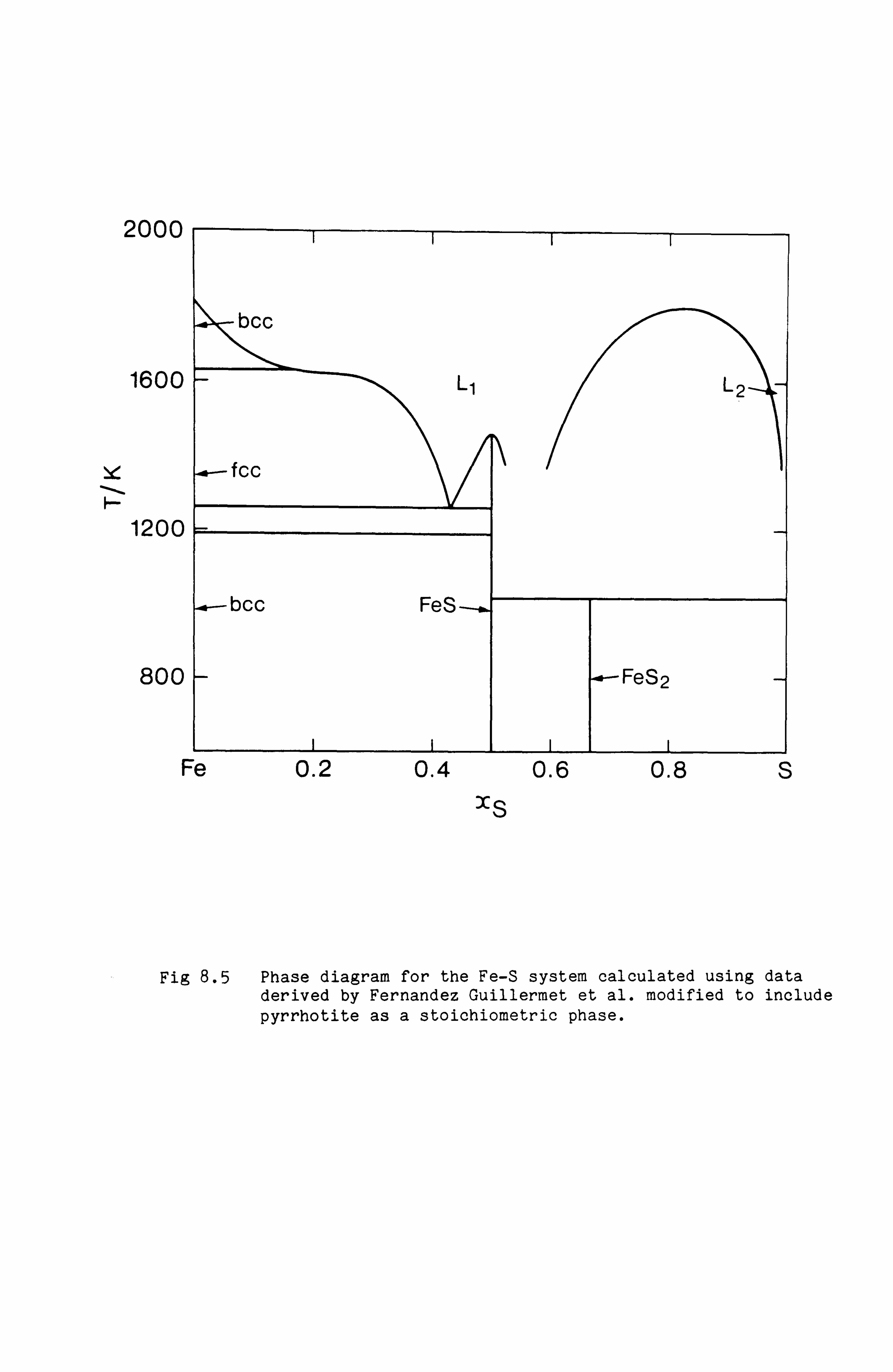
2000
1600
Y
H 1200
800
bcc
L1 L2
fcc
bcc FeS
FeS2
Fe 0.2 0.4 0.6 0.8 S XS
Fig 8.5 Phase diagram for the Fe-S system calculated using data derived by Fernandez Guillermet et al. modified to include
pyrrhotite as a stoichiometric phase.

2000
1500
Y H
1000
500
ýý L2 ý L3-4j
CU2S(S)
CuS Cu2S(ß)
Cu 0.2 0.4 0.6 0.8
xs S
Fig 8.6 Selected phase diagram for the Cu-S system.
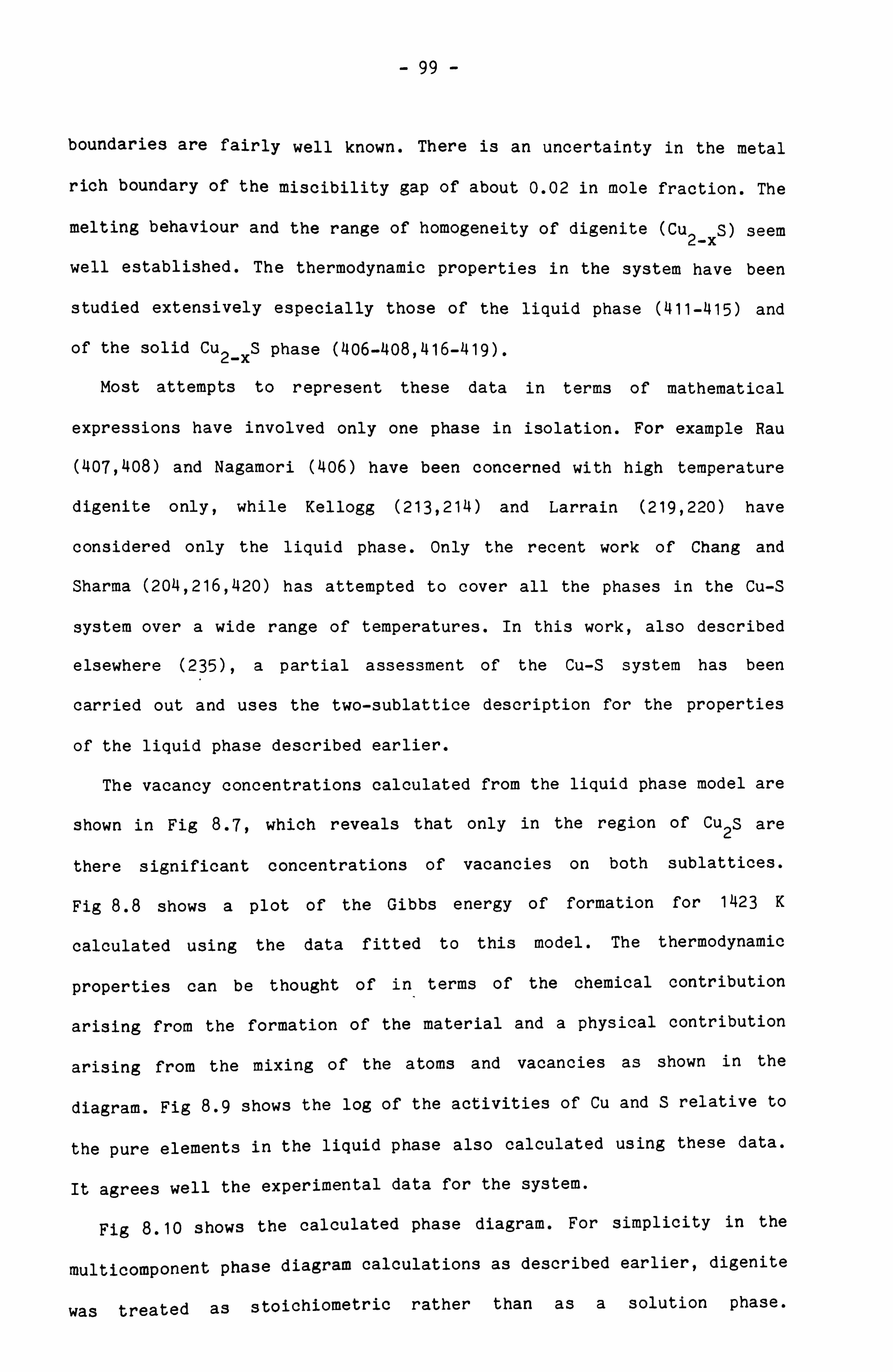
- 99 -
boundaries are fairly well known. There is an uncertainty in the metal
rich boundary of the miscibility gap of about 0.02 in mole fraction. The
melting behaviour and the range of homogeneity of digenite (Cu2_XS) seem
well established. The thermodynamic properties in the system have been
studied extensively especially those of the liquid phase (411-415) and
of the solid Cut-XS phase (406-408,416-419).
Most attempts to represent these data in terms of mathematical
expressions have involved only one phase in isolation. For example Rau
(407,408) and Nagamori (406) have been concerned with high temperature
digenite only, while Kellogg (213,214) and Larrain (219,220) have
considered only the liquid phase. Only the recent work of Chang and
Sharma (204,216,420) has attempted to cover all the phases in the Cu-S
system over a wide range of temperatures. In this work, also described
elsewhere (235), a partial assessment of the Cu-S system has been
carried out and uses the two-sublattice description for the properties
of the liquid phase described earlier.
The vacancy concentrations calculated from the liquid phase model are
shown in Fig 8.7, which reveals that only in the region of Cu2S are
there significant concentrations of vacancies on both sublattices.
Fig 8.8 shows a plot of the Gibbs energy of formation for 1423 K
calculated using the data fitted to this model. The thermodynamic
properties can be thought of in terms of the chemical contribution
arising from the formation of the material and a physical contribution
arising from the mixing of the atoms and vacancies as shown in the
diagram. Fig 8.9 shows the log of the activities of Cu and S relative to
the pure elements in the liquid phase also calculated using these data.
It agrees well the experimental data for the system.
Fig 8.10 shows the calculated phase diagram. For simplicity in the
multicomponent phase diagram calculations as described earlier, digenite
was treated as stoichiometric rather than as a solution phase.

0.004
c 0.003 0 f-+ U clö
LL
a) 0.002
U C co U
0.001 Copper sublattice
Sulphur sublattice
0- Cu 0.2 0.4 0.6 0.8 S
xs lmý
Fig 8.7 Fractions of vacancies on the copper and sulphur sublattices as a function of the overall composition calculated for 1423 K.

Cu-S 1423 K
T
O E
0
20
0
-20
-40
/ S. S.
Total Gibbs energy /
i
7
Cu 0.2 0.4 0.6 0.8
-º XS S
Fig 8.8 Contributions to the Gibbs energy of formation of the Cu-S liquid phase at 1423 K as a function of composition. The solid curve represents the total Gibbs energy of formation, the
upper dashed curve the contribution arising from mixing of atoms and vacancies and the lower dashed curve the
contribution from the formation of Cu2S when mixing is disregarded.

4
U
J
Cu,
-12 L Cu
Iý 1%6 000 f
0.2 0.4 0.6 0.8 S 1s -
Fig 8.9 The activities of Cu and S at 1423 K in the liquid phase of the Cu-S system. The dashed line refers to the region where the homogeneous liquid phase is metastable with respect to immiscibility.
0
-4
`ýý
000 //
*an. wasp
_g /
I S`

2000
1500
Y
F-
1000
500
Ll L2 L3
cuts (s)
cus cu2s(13)-..
Cu 0.2 0.4 0.6 0.8 S xS
Fig 8.10 Calculated phase diagram for the Cu-S system. The assumption that digenite has no range of homogeneity leads to slight discrepancies with Fig 8.6 on the sulphur rich side of Cu2S.

- 100 -
Consequently the liquidus curve to the sulphur rich side of digenite and
the eutectic at 1085 K have not been reproduced accurately. The
calculations in the metal rich part of the diagram indicate excellent
agreement with experimental information.
The Ni-S system
The Nickel-Sulphur system has been the subject of much experimental
study both from the point of view of the thermodynamic data and the
phase diagram.
The phase diagrams reported in Hansen and Anderko (53), Elliott (54),
Shunk (55) and the Metals Handbook (63) have been superseded by one
given by Craig and Scott (402). The metal rich part of the phase diagram
is dominated by a deep eutectic formed by the three phase equilibrium:
Liq = fee + beta
where the fee is basically Ni with a very small dissolved concentration
of S and beta is the solid solution phase based around the composition
Ni3S2, The structure of this beta phase is not at all well known being
apparently unquenchable and transforming on cooling to the low
temperature stoichiometric phase heazlewoodite (Ni3S2). There is some
evidence (383,386) to suggest that the beta phase consists of two
distinct phases of very similar thermodynamic properties. The other high
temperature phase in the metal rich part of the system is the
monosulphide Ni1_XS phase based upon the NiAs structure (B81). At low
temperatures, various stoichiometric phases appear. In addition to
Heazlewoodite there are: Ni7S6 (godlevskite), a low temperature form of
NiS (Millerite), Ni3S4 (Polydymite) and NiS2 (Vaesite). At high
temperatures the sulphur rich side of the system is dominated by a

- 101 -
liquid-liquid miscibility gap. The selected phase diagram shown in
Fig 8.11 is based upon that of Craig and Scott (402) but incorporating
additional information (378, L21-430).
The thermodynamic properties of the liquid phase have been determined
by a number of workers (378,379,421,422,431-437). The data from Meyer et
al. (378,379) are the most extensive and are to be preferred. Extensive
studies have also been carried out on the Beta phase or phases
(383,386,438-440) while Rau has also studied the monosulphide solid
solution (428). The low temperature stoichiometric phases have also been
studied (441-444). Data for the dilute solution of sulphur in nickel
have been derived by Brigham et al. (426).
Various authors have attempted to correlate the thermodynamic and
phase diagram data. Larrain (217) modelled the liquid phase using
species of Ni, Ni3S2 and NiS and obtained good agreement with the
liquidus at high Ni concentrations above 1000 K. However no other phases
were considered. Sharma and Chang (223) have, however, modelled all the
phases in the system and obtained excellent agreement between the
experimental and calculated phase diagram. For the liquid phase they
assumed an associated solution model with associate species of NiS. The
beta phases were modelled using an empirical power series for the excess
Gibbs energy while the Ni1_XS phase was modelled according to a
statistical thermodynamic model similar to that used for pyrrhotite
(221). The solubility of sulphur in pure Nickel was neglected.
For this assessment a two sublattice model, as described earlier, was
adopted for the liquid phase. The experimental data show a dramatic
change in the thermodynamic properties at about xS = 0.4 which led to
the adoption by Larrain of associated species of Ni3S2. However here it
was assumed that the most reliable description of the data using a two
sublattice model would be obtained by assuming that Ni had the same
valency as Sulphur ie. treating Ni-S liquid in the same way as Fe-S
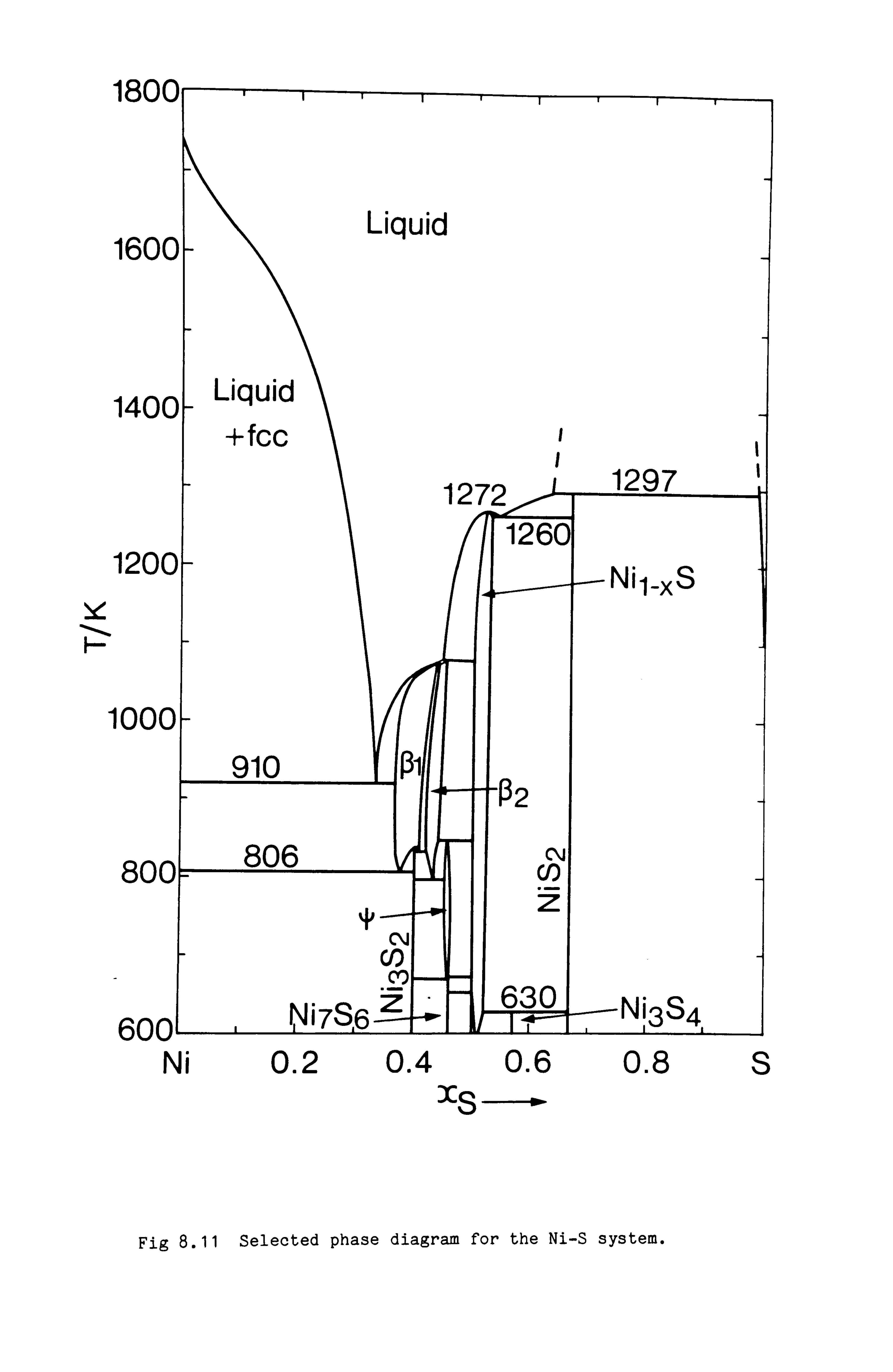
1800
160C
140C
1200
1000
800
inn
910
806
1272 1297
1260
F"P2
N
Z
N
C'7
i7S6 Z 630
Nil-XS
Ni3S4
Liquid
+ fc c
Liquid
vvv
Ni 0.2 0.4 0.6 XS ---- W.
0.8 S
Fig 8.11 Selected phase diagram for the Ni-S system.

- 102 -
liquid. As with previous assessments, liquid phase thermodynamic data
for various temperatures were fitted to the sublattice model. The final
agreement between the calculated and experimental partial pressures of
sulphur, compared in Fig 8.12, is excellent.
For reasons given earlier the solution of sulphur in solid nickel,
which at maximum is 0.001 in terms of mole fraction, was neglected.
Similarly the monosulphide phase Ni1_XS which has a range of homogeneity
from x9 = 0.5 to 0.52, has been treated as stoichiometric NiS.
The high temperature solid solution phase 'beta' based around Ni3S2
presented some problems. As mentioned earlier there is evidence which
indicates that the phase field consists of two distinct but similar
phases separated by a narrow two phase region. For simplicity this phase
field was treated as a single phase. The data were represented using a
simple . Redlich-Kister power series expression as used with success in
alloy systems. This model is not really appropriate and the data derived
for this phase, although acceptable, must be regarded as provisional.
Furthermore the data are applicable only for temperatures below 1150 K.
It is recommended that the phase should be reconsidered in terms of a
two sublattice description. The other phases in the metal rich part of
the system were treated as stoichiometric.
The phase diagram calculated from these data for Ni rich compositions
is shown in Fig 8.13.
Calculation of Phase Equilibria in the Cu-Fe-Ni system
Using data tabulated in the appendix, the phase diagram for the
Cu-Fe-Ni system was calculated by Chart et al. (169) using the NPL
ALLOYDATA system (15,173) between the temperatures 673 K and 1673 K.
They critically assessed experimental ternary phase diagram and
thermodynamic data for the temperature range 1023 K to 1523 K and

a
c, moo! - lop
CF) J-4
#4
Cr'
,o
+1
1 ce) ý
c 04
I
i i
.- cv m ýr tý
YI
I
M
m
N
C9
.
S
M tl- co
0
Cd
Lm «1ti ao
O C S. a) 4-1
"ý E L Q)
0. V) x W Cl)
Ci z
"v NN
CC U "rl
r-I co S. UC
aý a
a) w Ow
0 C 0 U)
"ý L LO cd V) M V) E Cu O L. Ua
N r-
[sue

1800
1600
1400
12 00
1000
800
600 L Ni
xs
Fig 8.13 The nickel rich part of the Ni-S phase diagram calculated using the critically assessed data.
0.2 0.4 0.6 0.8 S

- 103 -
incorporated them into the data set in the form of a temperature
dependent ternary interaction for the fcc phase. It is believed that the
need for a ternary interaction term arises from small errors in the data
for the Cu-Fe system. The agreement between the calculated and
experimental data is good and, it is believed, the optimised data set
provides a reliable means of extrapolation and interpolation in both
temperature and composition outside the range of experimental data.
Furthermore the data provide a reliable base for calculations of
equilibria in the Cu-Fe-Ni-S system.
Calculation of phase equilibria in the Fe-Cu-S system
According to Craig and Scott (402) 'more time and effort has been
expended in the determination of phase equilibria and minerological
relationships among the Cu-Fe sulfides than any other ternary sulfide
system'. They go on to say that despite this many aspects of the phase
diagram are unknown. This is hardly surprising in view of the large
number of ternary phases present in the system. Fortunately as far as
this work is concerned most of these ternary phases are stable only at
low temperatures and are in any case sulphur rich of the composition
line joining Cu2S and FeS. Fig 8.14 shows the experimental phase diagram
for the Fe-Cu-S system at 873 K from Chang et al. (74) based upon the
diagram of Cabri (445) and shows how the metal rich part of the phase
diagram is separated from the sulphur rich part by the two phase region
between Cu2S and FeS. This situation persists at lower temperatures.
Consequently for this work where all the compositions of interest are in
the metal rich region, all sulphur rich phases could be ignored.
The experimental work on the phase diagram of the Fe-Cu-S system has
been reviewed by Craig and Scott (402) and by Chang et al. (74,446)
which incorporate a considerable number of experimental measurements

S
0.8 ý /...:
xS
0.4
0.6 / Liq + Digenite
Cu-Fe-S 873 K
........ 0.2
Liq + Pyrite + fcc Pyrite
0.4 Fe
tcc
0.6
Digenite Digenite + Pyrrhotite +fcc + bcc
Pyrrhotite + bcc
0.2 .................. 0.8 Digenite + fcc + bcc
.....................:::......................:......................: v.....................:: i...................
Cu 0.8 0.4 0.2 0.6
-o- xcu
Fig 8.14 Experimental phase diagram for the Fe-Cu-S system for 873 K as assessed by Chang et al. The metal rich part of the phase diagram is separated from the sulphur rich part by the two phase region between digenite and pyrrhotite.
Fe
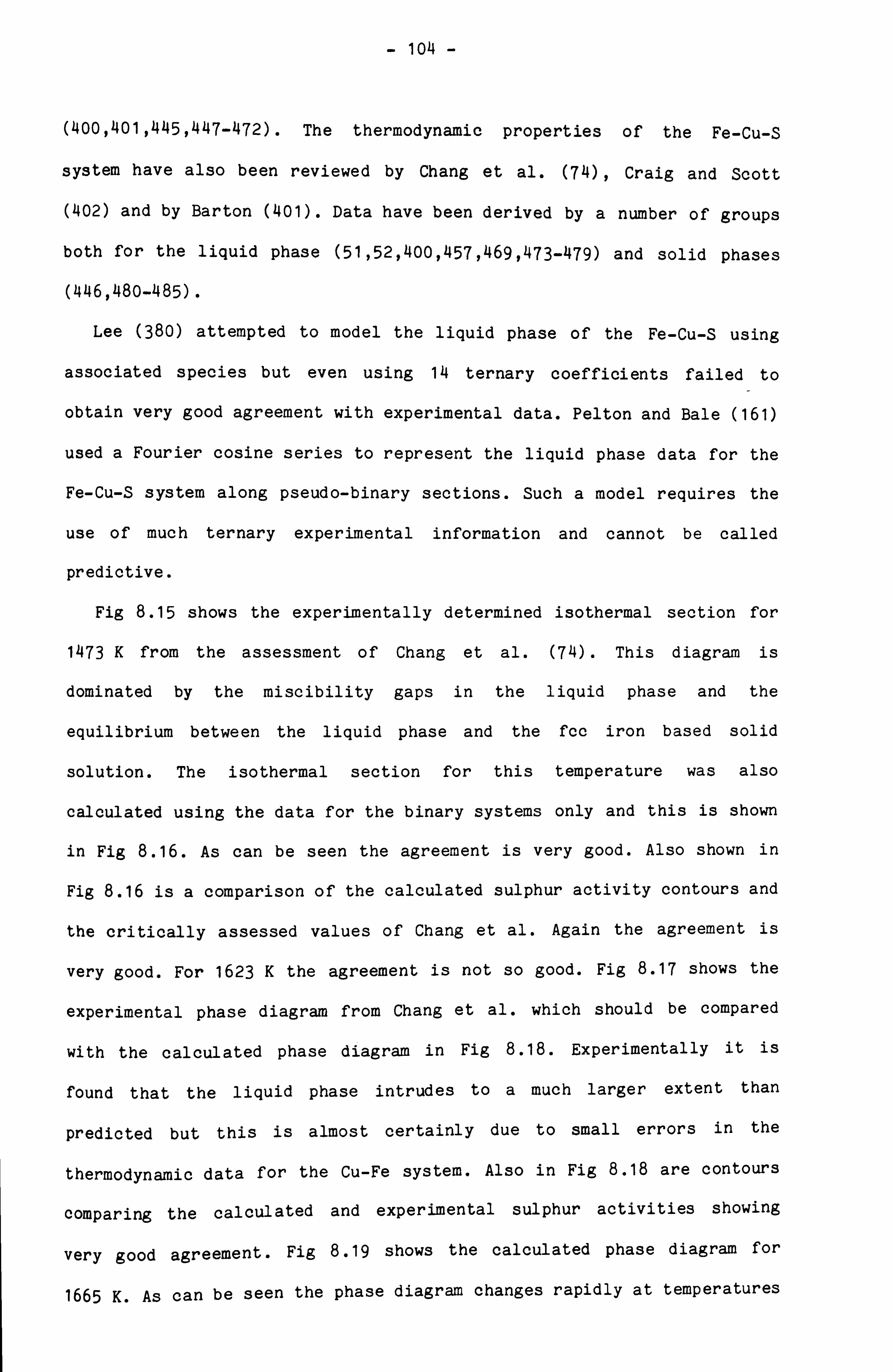
- 104 -
(400,401,445,447-472). The thermodynamic properties of the Fe-Cu-S
system have also been reviewed by Chang et al. (74), Craig and Scott
(402) and by Barton (401). Data have been derived by a number of groups
both for the liquid phase (51,52,400,457,469,473-479) and solid phases
(446,480-485).
Lee (380) attempted to model the liquid phase of the Fe-Cu-S using
associated species but even using 14 ternary coefficients failed to
obtain very good agreement with experimental data. Pelton and Bale (161)
used a Fourier cosine series to represent the liquid phase data for the
Fe-Cu-S system along pseudo-binary sections. Such a model requires the
use of much ternary experimental information and cannot be called
predictive.
Fig 8.15 shows the experimentally determined isothermal section for
1473 K from the assessment of Chang et al. (74). This diagram is
dominated by the miscibility gaps in the liquid phase and the
equilibrium between the liquid phase and the fcc iron based solid
solution. The isothermal section for this temperature was also
calculated using the data for the binary systems only and this is shown
in Fig 8.16. As can be seen the agreement is very good. Also shown in
Fig 8.16 is a comparison of the calculated sulphur activity contours and
the critically assessed values of Chang et al. Again the agreement is
very good. For 1623 K the agreement is not so good. Fig 8.17 shows the
experimental phase diagram from Chang et al. which should be compared
with the calculated phase diagram in Fig 8.18. Experimentally it is
found that the liquid phase intrudes to a much larger extent than
predicted but this is almost certainly due to small errors in the
thermodynamic data for the Cu-Fe system. Also in Fig 8.18 are contours
comparing the calculated and experimental sulphur activities showing
very good agreement. Fig 8.19 shows the calculated phase diagram for
1665 K. As can be seen the phase diagram changes rapidly at temperatures
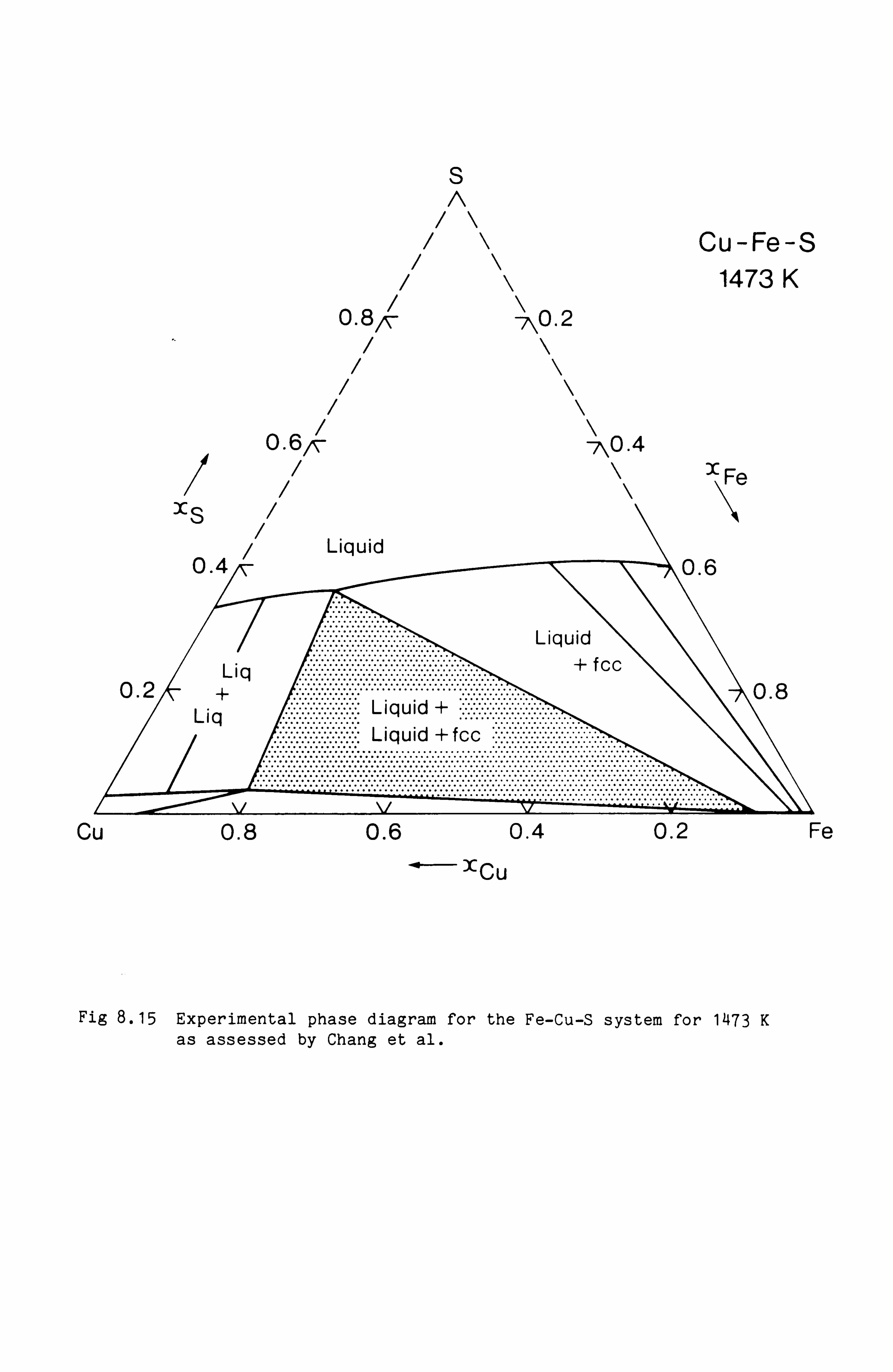
S n
Cu
/\ Cu-Fe-S 1473 K
0.8 0.2 /\
/\ /\
/\ 0.6/
NO. 4
//\\x Fe XS
/ Liquid 0.4 0.6
Liquid
Liq + fcc 0.2 + ........... 0.8
Liq Liquid + Liquid + fcc
0.8 0.6 0.4 0.2 Fe
xCu
Fig 8.15 Experimental phase diagram for the Fe-Cu-S system for 1473 K as assessed by Chang et al.

S n
Cu- Fe -S 1473 K
0.8ý X0.2 as
/ /
/ 0.6
-0.4
7x 10_3 \x Fe / Liquid
xs ew"o*
0.4 0.6
2x10⁻⁴ Liquid
+ fcc Liq
.......... ..... 0.8 0.2 + Liquid + Liq
Liquid + fcc
Cu 0.8 0.6 0.4 0.2
ý" XCu
Fig 8.16 Calculated phase diagram for the metal rich part of the
fn" 1I7' K_ suoerimoosed are experimental (short dash)
Fe
L' G -V to-v L va .. I . -. . ---r -- -+-
and calculated (long dash) sulphur activity contours.
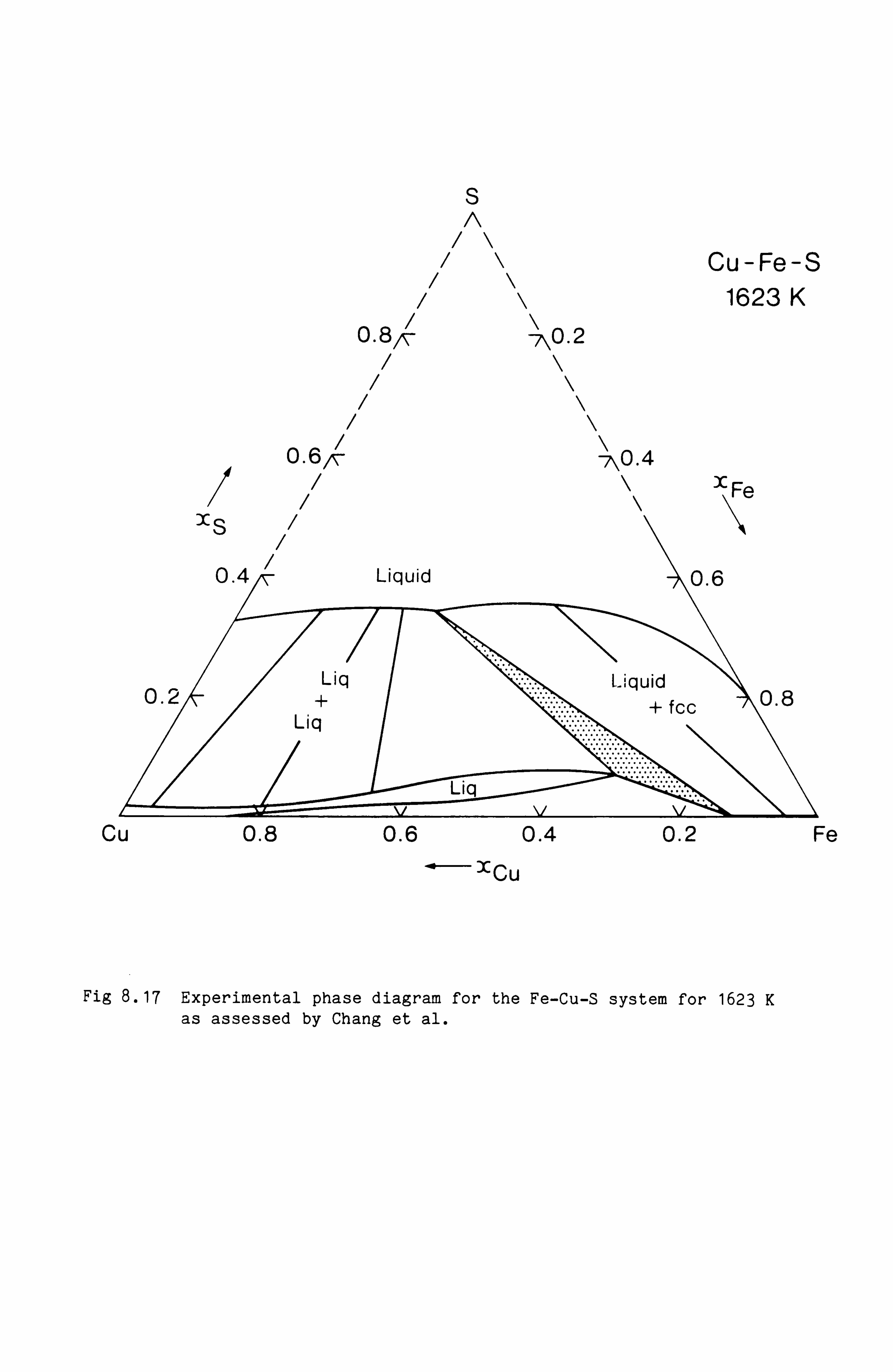
S n
ý Cu-Fe-S //
\\ 1623 K
0.8ý X0.2
0.6/, v X0.4
ýýx Fe
Cu 0.8 0.6
Q'ICU
0.4 0.2 Fe
Fig 8.17 Experimental phase diagram for the Fe-Cu-S system for 1623 K as assessed by Chang et al.
S n
/\ / Cu-Fe-S
1623 K 0.8t( N0.2 as
/ /
/ 0.6, -
1.4 x 10_2 7\0.4 / xFe
/ Liquid XS
0.4 0.6
3.4 x 10⁻⁴
Liquid Liq + fcc
0.2 + 0.8 Liq Liquid +
Liquid + fcc
Cu 0.8 0.6 0.4 0.2 Fe
-xcu
Fig 8.18 Calculated phase diagram_ for the metal rich part of the Fe-Cu-S for 1623 K. Superimposed are experimental (short dash) and calculated (long dash) sulphur activity contours.

S n
ý Cu-Fe-S 1665 K
0.8/v X0.2
} 0.6/, z- 7\0.4
ýýx FP
Cu 0.8 0.6
Cu 11 0.4 0.2 Fe
Fig 8.19 Calculated phase diagram for the metal rich part of the Fe-Cu-S system for 1665 K.
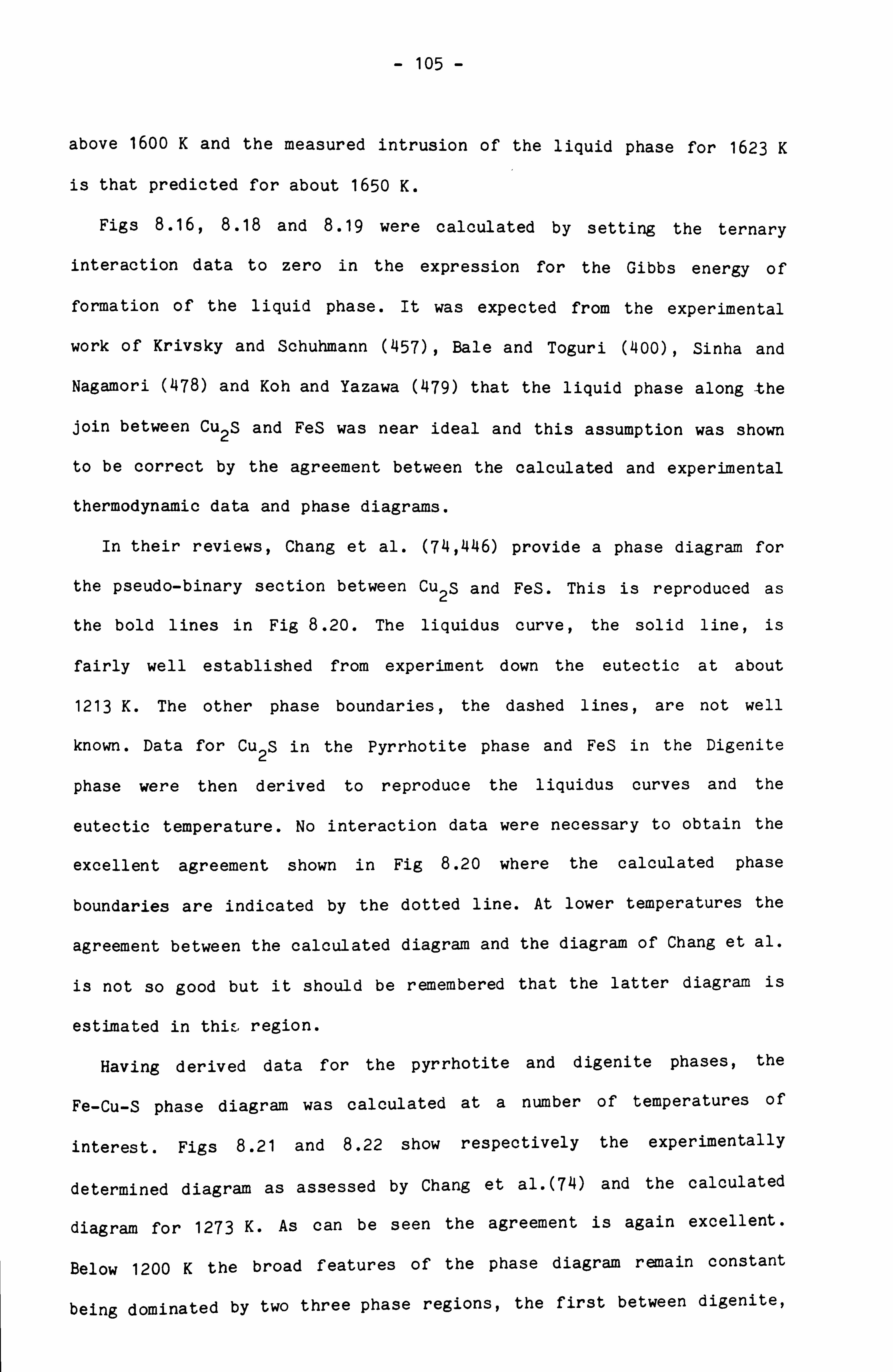
- 105 -
above 1600 K and the measured intrusion of the liquid phase for 1623 K
is that predicted for about 1650 K.
Figs 8.16,8.18 and 8.19 were calculated by setting the ternary
interaction data to zero in the expression for the Gibbs energy of
formation of the liquid phase. It was expected from the experimental
work of Krivsky and Schuhmann (457), Bale and Toguri (400), Sinha and
Nagamori (478) and Koh and Yazawa (479) that the liquid phase along -the
join between Cu2S and FeS was near ideal and this assumption was shown
to be correct by the agreement between the calculated and experimental
thermodynamic data and phase diagrams.
In their reviews, Chang et al. (74,446) provide a phase diagram for
the pseudo-binary section between Cu2S and FeS. This is reproduced as
the bold lines in Fig 8.20. The liquidus curve, the solid line, is
fairly well established from experiment down the eutectic at about
1213 K. The other phase boundaries, the dashed lines, are not well
known. Data for Cu2S in the Pyrrhotite phase and FeS in the Digenite
phase were then derived to reproduce the liquidus curves and the
eutectic temperature. No interaction data were necessary to obtain the
excellent agreement shown in Fig 8.20 where the calculated phase
boundaries are indicated by the dotted line. At lower temperatures the
agreement between the calculated diagram and the diagram of Chang et al.
is not so good but it should be remembered that the latter diagram is
estimated in this region.
Having derived data for the pyrrhotite and digenite phases, the
Fe-Cu-S phase diagram was calculated at a number of temperatures of
interest. Figs 8.21 and 8.22 show respectively the experimentally
determined diagram as assessed by Chang et al. (74) and the calculated
diagram for 1273 K. As can be seen the agreement is again excellent.
Below 1200 K the broad features of the phase diagram remain constant
being dominated by two three phase regions, the first between digenite,
2000
1500
Y
F-
1000
�'
/ /
/ I
/ / I I.........
ýr
. 'i
1
1
:1
5001 CU2S 0.1 0.2 0.3 0.4 FeS
X Fe
Fig 8.20 Pseudo-binary section between Cu S and FeS showing the
calculated (dotted line), experiýental (solid line) and assessed (dashed line) phase boundaries.
1, ýr. ý ýýý
,. ý. vV, "mit
" ... ý"`,
_ .

S Liquid
Cu-Fe-S 12 73 K
Digenite
Digenite + fcc -
0.2,
Pyrrhotite X Fe
Cu 0.8 0.6 0.4 0.2 Fe
'-- xcu
Fig 8.21 Experimental phase diagram for the Fe-Cu-S system for 1273 K
as assessed by Chang et al.

S n
0.8ý
0.6
/ Digenite Is + Liquid
Digenite 0.4 /7 /
\ \
\ \ XO. 2
Pyrrhotite X0.4
+ Liquid�
Liquid
Cu-Fe-S 1273 K
x Fe
0.6
Digenite Liquid + fcc + fcc
0.2 .........
Digenite + .......... 0.8
fcc + fcc
.................. . ýc: ý : :::...... %:::::::::::::.....:: :::::: ý i:: ::: ............
Cu 0.8 0.6
~xCu
0.4 0.2 Fe
Fig 8.22 Calculated phase diagram for the metal rich part of the Fe-Cu-S system for 1273 K.
- 106 -
fcc and bcc and the second between digenite, pyrrhotite and bcc as shown
in Fig 8.23, the phase diagram for 973 K.
Calculation of phase equilibria in the Ni-Cu-S system
The phase diagram of the Ni-Cu-S system has also been the subject of
much study and this work has been reviewed by Chang et al. (714). As
Kullerud and Moh (486) pointed out, the high temperature phase diagram
is dominated by three separate homogeneous liquid regions as in Cu-S
binary system. The miscibility gap between the matte phase and the metal
rich liquid phase has been studied by a number of groups
(380,381,487-490) of which, according to Chang et al. the data of
Schlitt et al. (487) and Lee et al. (380,381) are the most reliable. A
number of investigations of the phase diagram have been made for lower
temperatures (429,466,488,491-496).
Thermodynamic data for dilute solutions of sulphur in liquid
copper-nickel alloys have been tabulated by Chang et al. (74). For more
concentrated liquids data have been determined by Sryvalin and Esin
(497), Matousek and Samis (498) and Lee et al. (380,381).
Two groups have thus far attempted to represent the thermodynamic
data for the Ni-Cu-S system and check their assessments for consistency
with the phase diagram. Both groups considered only the liquid phase and
its equilibrium with the Ni-Cu fcc phase. Larrain and Lee (382) used an
associated solution model with species of Cu, Cu2S, CuS, Ni, Ni3S2 and
NiS with a large number of ternary interaction parameters to represent
the liquid phase and they obtained excellent agreement with all the
experimental information. Chuang and Chang (381) also used an associated
solution model for the liquid phase with species of Cu, Cu2S, S, Ni and
NiS, and derived the six temperature dependant ternary interactions
between the species from the data for the binary system. Their

S n
i i
i o. 8
i
0.6IV
xS / Digenite /
0.4, z
Digenite + Pyrrhotite
Cu-Fe-S 973 K
X0.2
\0.4
Pyrrhotite Fe
: "::: ":: Digenite+:.: \ + 0.6 ':: '' Digenite:::: Pyrrhotite ::
+ bcc + bcc Pyrrhotite Digenite + bcc
................................. ................... ................................. .................. + fcc
0.2 Digenite + ........... .......... ... ... 0.8
fcc + bcc
-XU
Cu 0.8 0.6 0.4 0.2 Fe
4- 'ICU
Fig 8.23 Calculated phase diagram for the metal rich part of the Fe-Cu-S system for 973 K.

- 107 -
representation of the available data, while it is very good, is not so
good as that of Larrain and Lee but then they used fewer parameters.
As for the calculations of the Fe-Cu-S system, high temperatures were
considered first. For the Fe-Cu-S system it was shown that the two
sublattice model was able to represent the thermodynamic data for the
liquid phase without the need for any ternary interaction data.
Tentative phase diagram calculations were made for the miscibility gap
in Cu-Ni-S system at 1473 K and 1673 K without any ternary interaction
data and it was found that the agreement between calculated and
experimental phase diagram was poor. This produced a phase diagram where
the miscibility gap in the liquid phase extends much too far into the
ternary system from the Cu-S binary compared with the experimental
diagram shown in Fig 8.24. Ternary interactions were introduced into the
liquid phase data set in order to improve the agreement between the
calculated and experimental phase diagrams. Fig 8.25 shows the
calculated phase diagram with the experimental phase boundaries
superimposed. The agreement is acceptable although it is recommended
that more work should be done in the future to improve the agreement.
Figs 8.26,8.27 and 8.28 show the calculated partial pressures of
sulphur expressed as log(p3 2
)/2 for 1473 K and 1673 K for pseudo-binary
cuts through the ternary system corresponding to constant xNi: xCu ratios
of 3,1 and 0.333 respectively. Superimposed on these curves are the
experimental data of Lee et al. (380,381). The agreement is very good
for Ni rich compositions. For Cu rich compositions the agreement is not
so good and this explains the disagreement between the calculated and
experimental miscibility gap phase boundaries which are very sensitive
to small changes in the thermodynamic data. Extra terms could have been
introduced into the liquid phase data set to obtain better agreement but
this would have impaired the predictive power of the model. It is
believed that the cause of the discrepancy lies in the choice of the

S
i
Cu 0.8 0.6 0.4 0.2 Ni
IN 'ICU
Fig 8.24 Experimental metal-matte miscibility gap in the Ni-Cu-S system for 1473 K as assessed by Chang et al.

S A
0.8 ý ý. 0.2
0.6
Cu
'Cu
Fig 8.25 Calculated phase diagram for the metal rich part of the Ni-Cu-S system for 1473 K. The experimental metal-matte miscibility gap is superimposed as the dashed line.
Ni-Cu-S 1473 K
40.4 ýý ýc Ni
Ni V. V %-# .V%. 0 .T tcc r
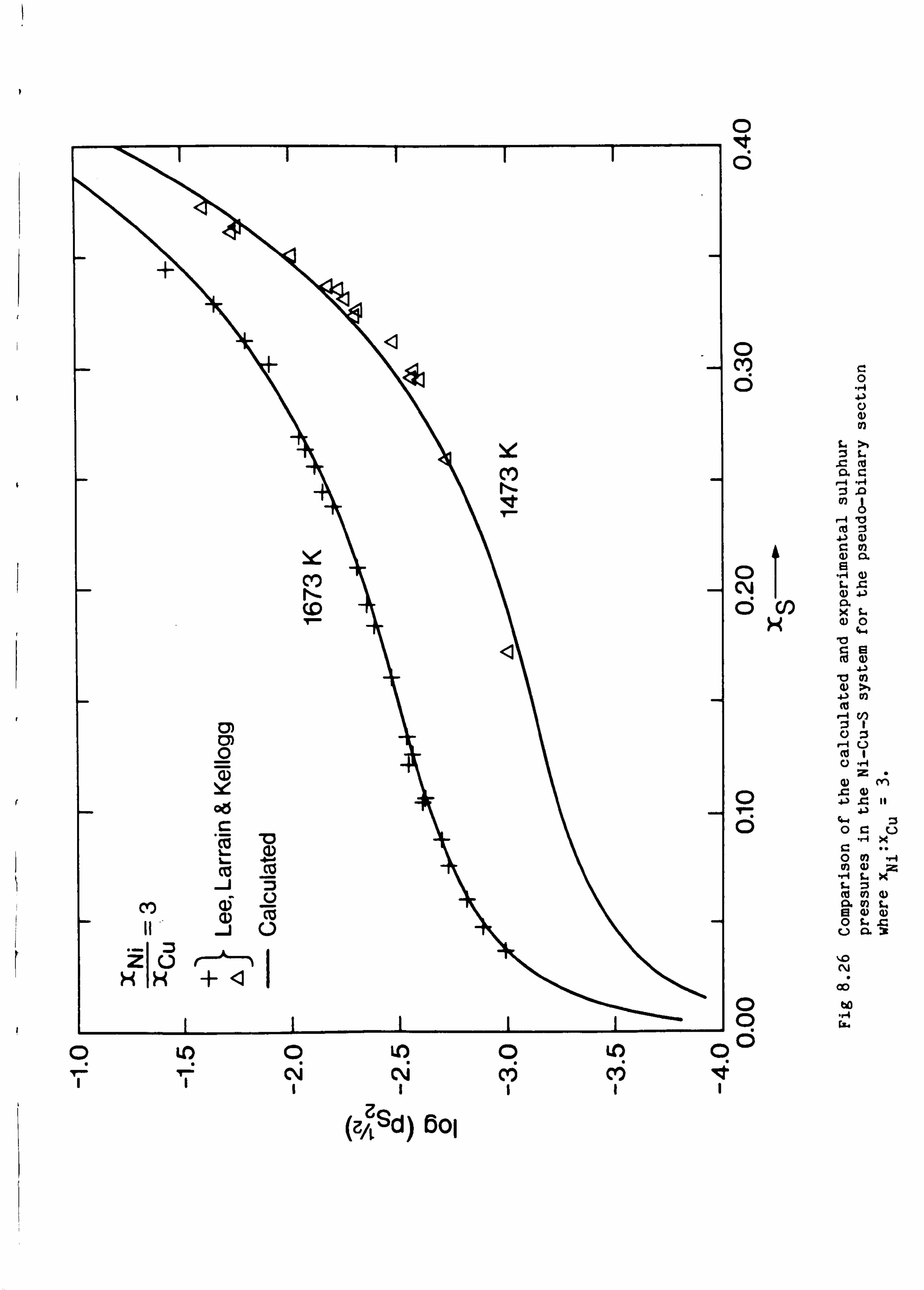
+
V co ti (0 T-
a) 0) 0 75 Y CO c
c J ý
Ü II i
4
0 LI) O LO rNN
(z%Sd) 601
Y Cý) N- T
0 It ö
O C1) Ö 0
C) G) C1
t» ý O t.
aC
1-4 b C in aý a
O ß aß N
v/ K
i. °'w
0 43 bm
c1 a1 UO
. -I U cd 1 C) "rl
Z G) M
O ý.. 1
,C 11 1 O OC
O v) rl
cd V1 C) 6 9)
Q OL c) a
N
00
O m O ýr
o ýn o0 M

+
+
+
+ 4
a Y Cl) N.
D I D
0 o 0
. r., 4) 0 (1) 00
L ?,
a C13 c
.n 0
co "v te c a)
an O E Cl.
N e ý
C5 O) LJ (l
>C N
L O
4-4
c e
b a)
ca
cd U "r1
O ýC: U
r--
T 4i 4)
11
O 4-4 O c
z U
r4 >C
O (n
v) a)
"rl z
"r L x
co vn d)
(L) L
e o O) L (1) C U a 3
ti N
o cc
O bo "C4 CL4
++ * ad
Y
ti a (D
0 Y+Q 015 c
C J
rýV
il JÜ
ZÜ ýý
p In o 7N N
I
(Sd) 60l
0I00

M ti
Y r" M CD + q-
a co C7
U N
2
T--
0) D) O Y
ad c
+
+ +
J
(f1 J U
O co
(0
CV) N.
Ü I K H +4
O r
1
to 0 LO NN
(z%Sd) 6oß
0 ö
O (") C
0
U
U)
>1 7 C.
.C cd ß. C
-l "ý 7 .D
(1) a C V) au a o 4
O (f) C. '' (D 0
a CB
CO >1 O
cd r-1 (n
Ua
cd 1 U "r1 Z
Q G) CN
M
11
OC 2 x C ýý 0 U) :3 U) G) U
1 L. X i. 7 ab V1 C)
E Q) O O C. .C Ua
co N
0 O O0
_ [z
o ýn o° M

- 108 -
notional charge for Ni as 2. A value of 1.333, as implied from the
thermodynamic data would probably allow better extrapolation into
ternary systems. It should however be remembered that the representation
of the Ni-S binary thermodynamic data by the present data set is very
good as shown in Fig 8.12.
Fig 8.29 again shows the calculated phase diagram for 1473 K but,
with superimposed, the contours for constant activity of sulphur. Fig
8.30 shows the experimental diagram for the Ni-Cu-S system at 1673 K
which should be compared with Fig 8.31, the calculated diagram. In
Fig 8.32, the calculated diagram is shown with contours representing
constant sulphur activity expressed as log(ps )/2. Figs 8.33 and 8.34 2
show the calculated phase diagram for 1273 K and 1173 K respectively.
They show the gradual disappearance of the matte-liquid metal
miscibility gap, the formation of the digenite and pyrrhotite phases,
the increasing dominance of the three phase region Liq + fcc + Digenite
and the formation of the beta phase based around the composition Ni3S2.
Data for NiS in the digenite phase and interaction parameters for both
the digenite and pyrrhotite phases were derived in order to obtain best
agreement with the experimental diagram for 1053 K from Chang et al.
(74) shown in Fig 8.35. In a similar way data for the Cu-S, Cu-Ni and
ternary Cu-Ni-S interactions in the beta phase were derived to be
consistent with Fig 8.35. The calculated diagram is shown in Fig 8.36.
The results for the sulphur rich part of the system should be ignored
for the purposes of comparison. The calculated phase boundaries are in
some disagreement with the experimental boundaries, in particular the
composition of the fcc phase at the corner of the three phase region
with liquid and digenite, and the boundaries of the liquid phase in
equilibrium with digenite and fcc. It is felt however that the
calculated diagram is likely to be more correct. Fig 8.37 shows the
calculated diagram for 973 K close to a predicted eutectic between

S n
0.8k -ý0.2
0.6k -ý0.4 /\
x S/
-1.0 - _s- ----2.0- --
Ni-Cu-S 1473 K
3CNI
0.6
-2.5------- - 2.65------
0.2 ____-3.0----
Cu 0.8 0.6 0.4
4- X cu
0.2
Fig 8.29 Calculated phase diagram for the metal rich part of the Ni-Cu-S system for 1473 K with contours for constant sulphur activity expressed as log(pS )/2.
2
0.8
Ni

S
1
CU 0.8 0.6 0.4 0.2 Ni
a1 Cu
Fig 8.30 Experimental metal-matte miscibility gap in the Ni-Cu-S system for 1673 K as assessed by Chang et al.

S n
ý Ni-Cu-S 1673 K
0.8 0.2
0.6( ý 0.4 ý
ýý XNi
Cu
-1Cu
Ni
Fig 8.31 Calculated phase diagram for the metal rich part of the
- Ni-Cu-S system for 1673 K.
V. V V. V v"T -. -0 . 46- tcc

xs
S n
0.8 k-0.2
0.6 kX0.4
/\
Cu 0.8 0.6 0.4
IxCu
0.2
Ni-Cu-S 1673 K
XNi
Fig 8.32 Calculated phase diagram for the metal rich part of the Ni-Cu-S system for 1673 K with contours for constant sulphur activity expressed as log(pS )/2.
2
Ni
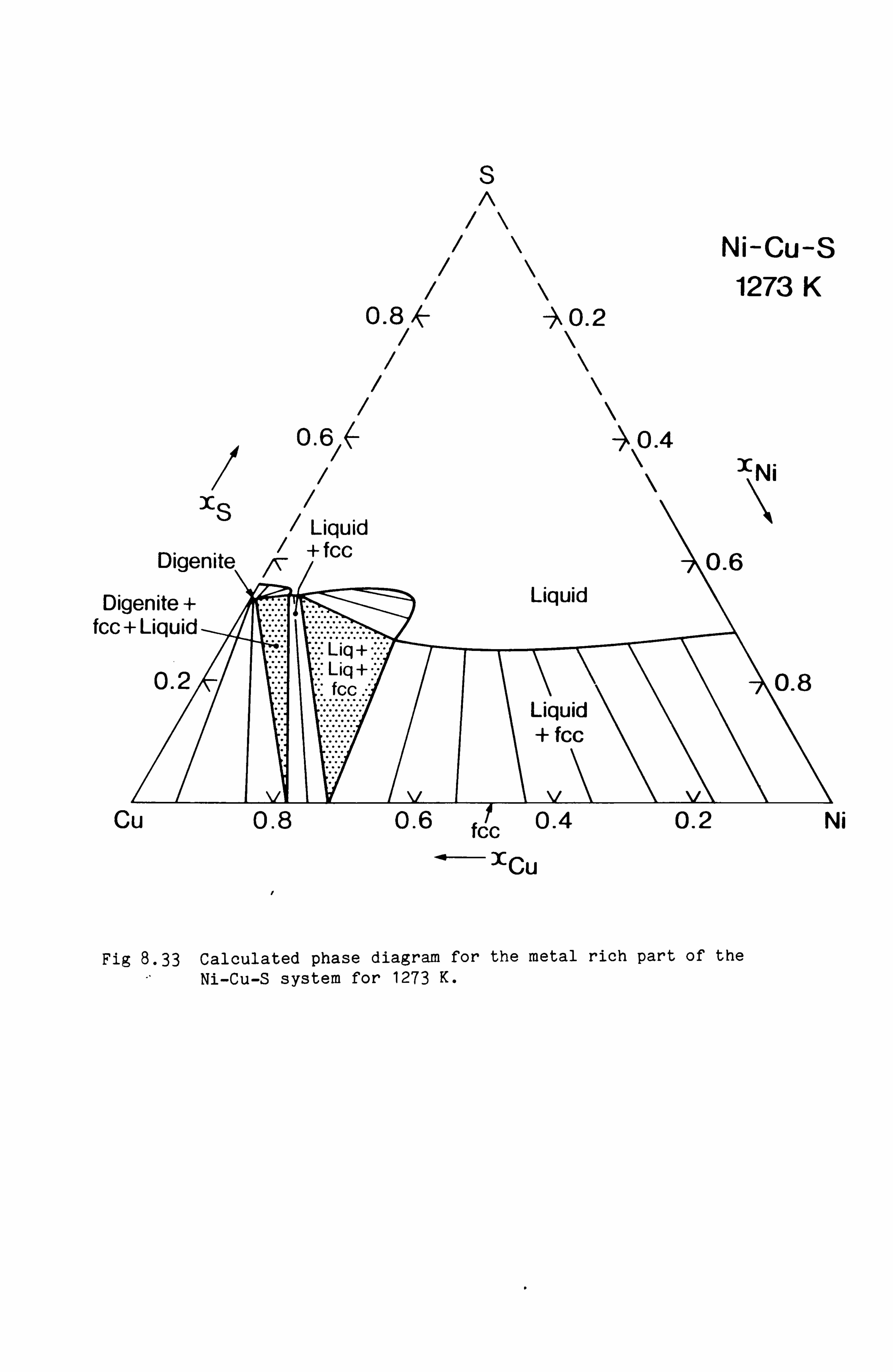
S A
/\
0.8 0.2
0.6 -ý 0.4
xs / / Liquid /+ fcc Digenite '- ý
Digenite + Liquid fcc + Liquid
Liq+
0.2 Liq+ fcc
Liquid + fcc
Cu 0.8 0.6 fcc 0.4
'-- xCu
Ni-Cu-S 1273 K
ýNi
0.6
0.2
0.8
Ni
Fig 8.33 Calculated phase diagram for the metal rich part of the Ni-Cu-S system for 1273 K.

S A
/\ /\
/\ 0.8ý 30.2
/\ /\
/\
0-6/( 4 0.4 Pyrrhotite
XS Liq +Liq + Digenite
Digenite /V Liq+Liq Liquid
Liq+fcc+..
02 Digenite fcc + Liquid
Digenite + fcc
Cu 0.8 0.6 fcc 0.4
40 xCu
Ni-Cu-S 1173 K
ýcNI
0.6
0.8
0.2 Ni
Fig 8.34 Calculated phase diagram for the metal rich part of the
Ni-Cu-S system for 1173 K.
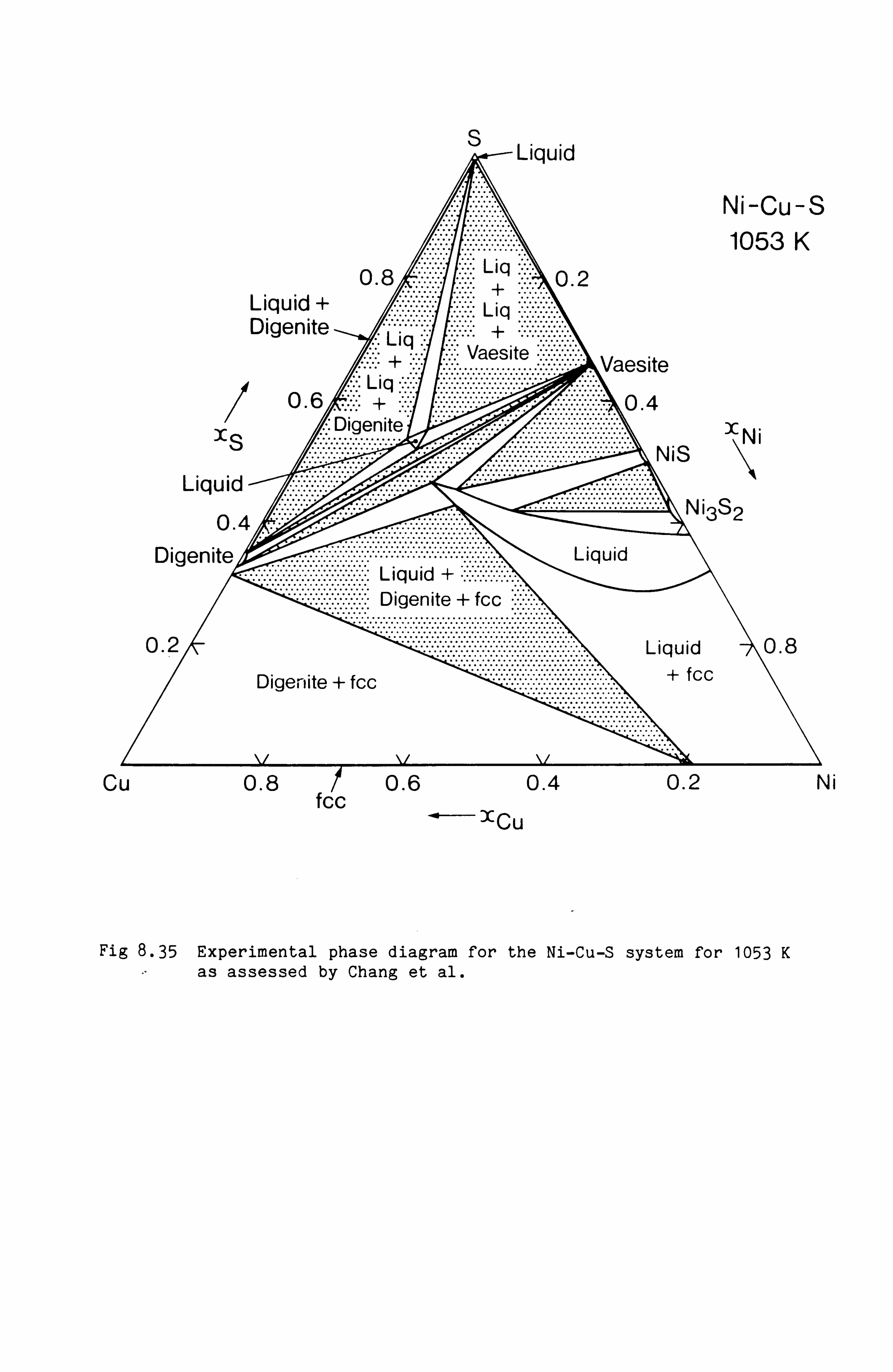
Liquid
0. s Liquid + Digenite . Li.
0.6
Ni-Cu-S 1053 K
Liq 0.6
.. +0.4 x Digenite "XNi
S NiS Liquid
Ni3S2 0.4
Digenite """""""""""" Liquid Liquid + ......... Digenite + fcc
0.2 Liquid
Digenite + fcc + fcc
Cu 0.8 fcc
Liq 0.2 Liq
aesite Vaesite
0.4
. -1Cu
0.2
0.8
Ni
Fig 8.35 Experimental phase diagram for the Ni-Cu-S system for 1053 K as assessed by Chang et al.
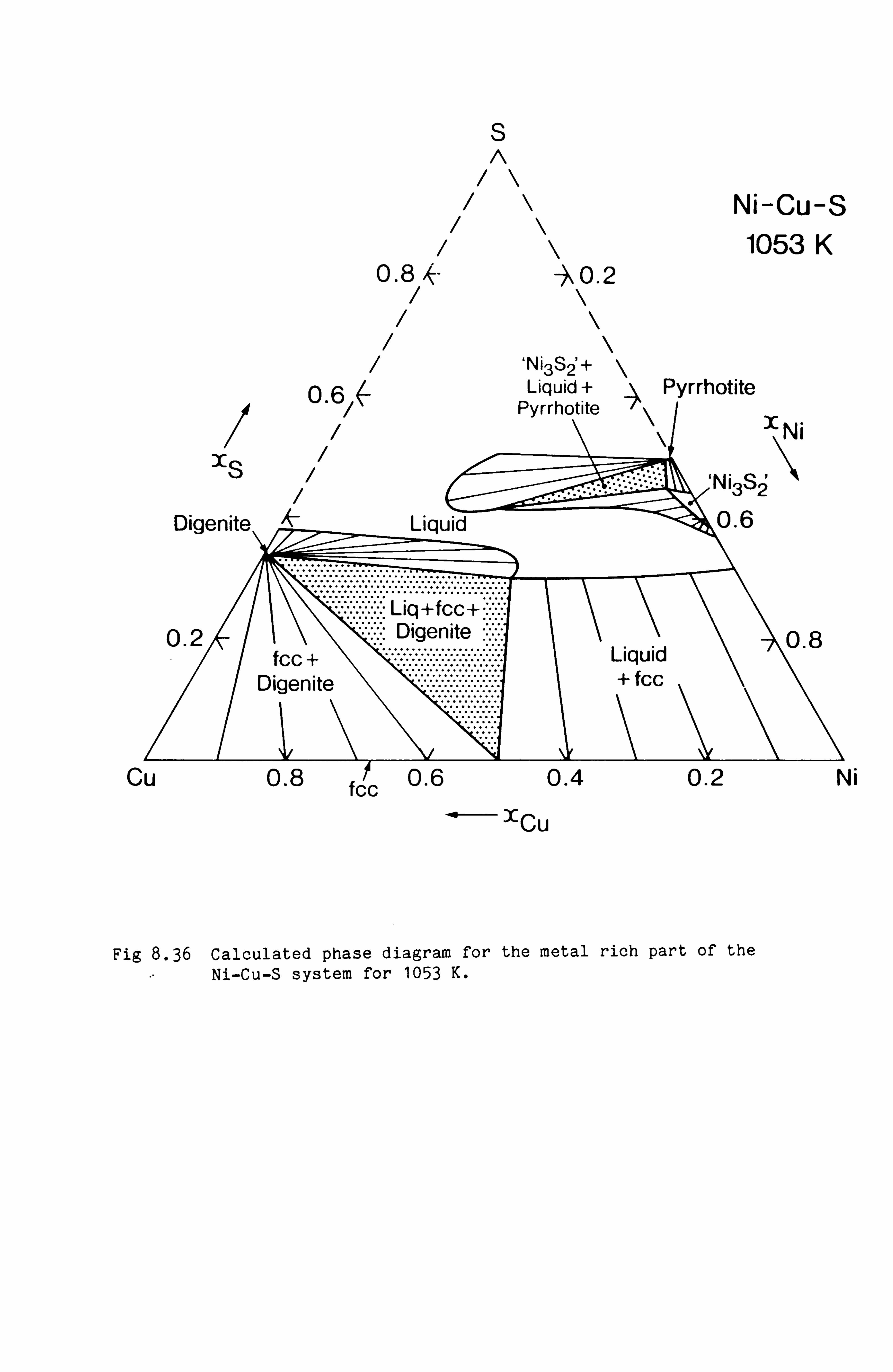
S n
/\
0.8 k- 0.2
`Ni3S2'+ \
Ni-Cu-S 1053 K
n r, 4 Liquid +, Pyrrhotite Pyrrhotite
xs
Digenite
0.2
Cu
Liquid
Liq+fcc+: Digenite
fcc + Digenite
0.8 fT0.6 0.4
~- xCu
Liquid + fcc
XNi
, 'N '3S2
0.6
0.2
0.8
Ni
Fig 8.36 Calculated phase diagram for the metal rich part of the Ni-Cu-S system for 1053 K.

S A
/\
0.8* 30.2
`Ni3S2 +\
Ni-Cu-S 973 K
naL Liquid +A Pyrrhotite -71 Pyrrhotite
xs / Liquid
Digenite
Liquid
Liq+fcc+ 2 Digenite
fcc + Liquid Digenite + fcc
Cu 0.8 0.6 fc0.4 ~xCU
xNi
`N i3S2
X0.6
0.8
0.2 Ni
Fig 8.37 Calculated phase diagram for the metal rich part of the Ni-Cu-S system for 973 K.

- 109 -
digenite and the beta phase. This is in excellent agreement with the
experimental eutectic temperature of 978 K (7,! 88). Fig 8.38 shows the
calculated phase diagram for 873 K and this should be compared with the
experimental phase diagram in Fig 8.39. A ternary eutectic is predicted
from the calculations and this has been observed experimentally. The
overall agreement between Figs 8.38 and 8.39 is very good.
Calculation of phase equilibria in the Ni-Fe-S system
The Ni-Fe-S system is of great general interest since phases based in
this system are found in many ores. The experimental data for the
Ni-Fe-S system has been reviewed by Hsieh et al. (499) and Craig and
Scott (402) incorporating the large number of studies of the phase
diagram (466,500-520).
There have been few experimental studies to derive thermodynamic data
for the Ni-Fe-S system. Naldrett and Craig (506) and Kao (517) have
studied the partial pressure of sulphur above the monosulphide solid
solution (pyrrhotite). Kao, who also studied the two phase region
between pyrrhotite and the beta phase, paid particular attention to the
phase relationships and the representation of the thermodynamic data.
Scott et al. (521,522) investigated the activity of FeS in the
pyrrhotite phase at 1203 K and found that NiS and FeS mix ideally for a
given mole fraction of sulphur. Studies have been carried out on dilute
solutions of sulphur in the liquid phase (432-434,523,524). Concentrated
liquids have been studied by Vaisburd et al. (525) who measured the
activities of Fe in cc, - entrated liquids at 1573 K while Byerley and
Takebe (437), Meyer (379) and Bale (526) have studied the partial
pressures of sulphur above the liquid phase at high temperatures.
Thermodynamic data were predicted for the liquid phase from the data
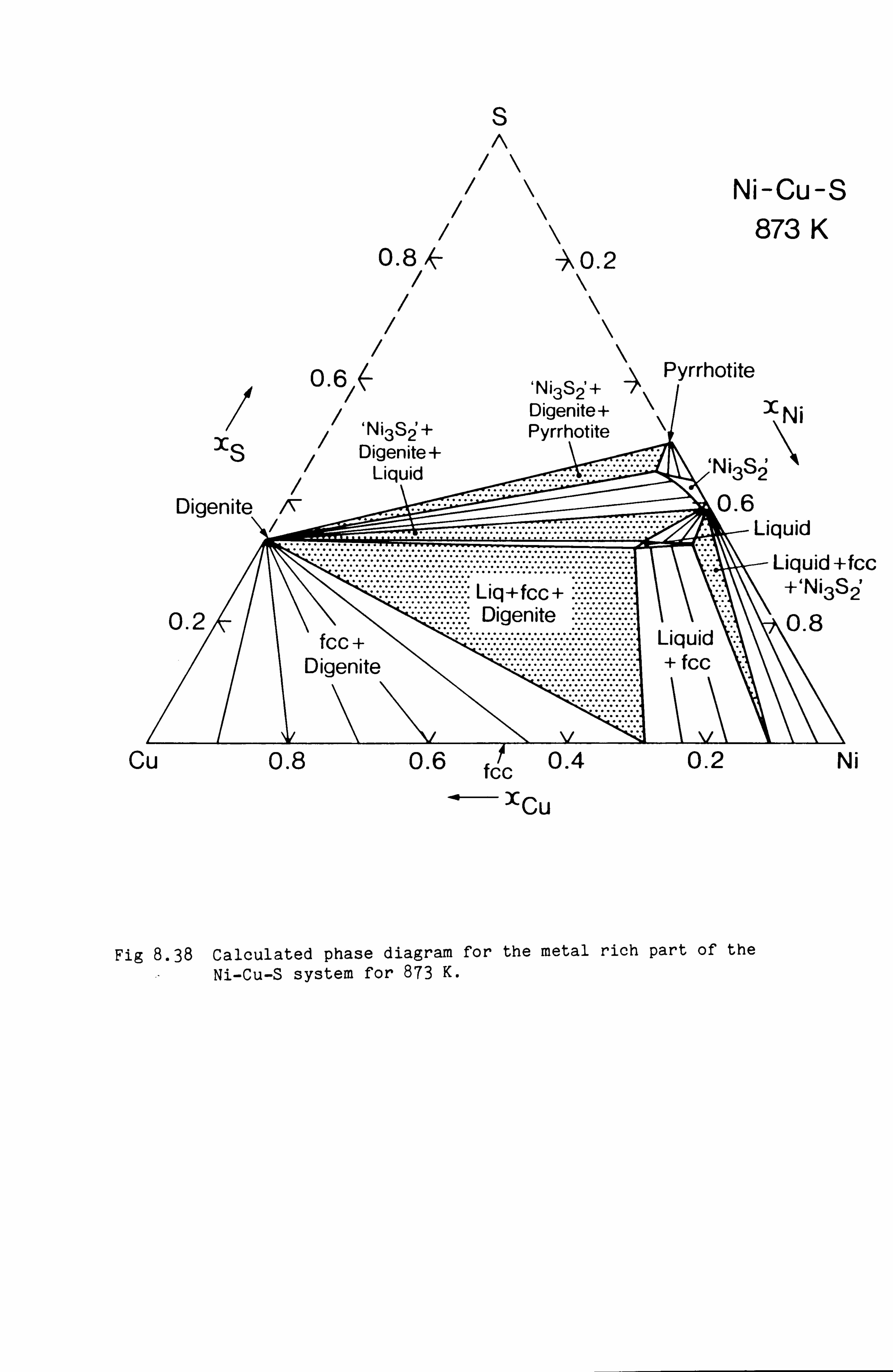
xs
Digenite
0.2
Cu
S A
/\
0.8 A- 30.2
0.6 `Ni3Si+ Digenite+
`Ni3S2 + Pyrrhotite Digenite+
Liquid
Ni -Cu -S 873 K
Pyrrhotite
1Ni
, N'3S2
0.6 .............................. ...............
Liq+fcc + Digenite
fcc + Digenite
0.8 0.6 fT0.4 ~ XCu
Liquid +fcc
Liquid
- Liquid +fcc +'Ni3S2
0.8
0.2 Ni
Fig 8.38 Calculated phase diagram for the metal rich part of the Ni-Cu-S system for 873 K.

Al Liquid
0 .......... 0.2 Liquid
Digenite Vaesite Vaesite
........................... ................ 0.6 0.4
Digenite + Vaesite+NiS NiS xS
0.4
Digenite ........................
Liquid + Digenite 0.2 + fcc
Digenite + fcc
Cu 0.8 fcc
0.6
.4 XCu
0.4
Ni - Cu- S 873 K
xNi
Ni3S2
Liq
fcc
0.2
Fig 8.39 Experimental phase diagram for the Ni-Cu-S system for 873 K as
Liquid
0.8
Ni
assessed by Chang et al.

- 110 -
of the component binary systems only. As was found for the Cu-Ni-S
system these predicted data were not in good agreement with the
available experimental data and it was necessary to introduce ternary
parameters. The data of Byerley and Takebe are thought to be less
reliable than those of Meyer and Bale and have not been considered in
detail. Some reliable phase diagram data are also available for the
equilibrium between the liquid phase and fcc metallic phase (516).
Close agreement between predicted and experimental thermodynamic and
phase diagram data was obtained by optimising the ternary parameters
with a specially developed computer program. Figs 8.40,8.41 and 8.42
show the calculated partial pressures of sulphur and, superimposed, the
experimental values determined by Meyer (379) for 1473 K, 1573 K and
1673 K and various relative proportions of Fe and Ni. Fig 8.43 shows the
calculated partial pressures of sulphur for various relative proportions
of Fe and Ni at 1473 K with the experimental data of Bale (526)
superimposed. As shown the agreement between calculated and experimental
data is very good. There does however seem to be some disagreement
particularly for high relative ratios of iron to nickel.
Figs 8.44 and 8.45 shows the calculated phase diagram for 1573 K and
1473 K in good agreement with the experimental work of Lenz et al.
(516). The calculated phase diagram for 1473 K is also shown in Fig 8.46
with contours representing constant activities of sulphur expressed as
log(p3 )/2. 2
Below 1464 K the pyrrhotite phase becomes stable first for the
composition FeS and at lower temperatures extending completely across
the system to NiS. According to Scott et al. (521,522) who measured the
variation of the activity of FeS in the monosulphide solid solution, FeS
and NiS mix ideally at 1203 K. Furthermore Misra and Fleet (513-515) and
Craig (512) found that at temperatures below 573 Ka miscibility gap
develops either side of a composition corresponding to FeNiS2. These two

(z/ýSd) 60l
0 lf) d
0
O
0 co ö
0 N 6
Jo Ir- o°
iý
c 0 4 OL
LN 4) ý U] A
. C" N CL >, £ rl L : ci e rn c0
"rI L ý ,aw cd I
O cd c "v (D cd e a) v rm La r-1 a) cd a cd +) X s~ NL a)
O "v 6, r-1 CL Cd EO
aý a "v+- x aý ýn w cu vý
' -I N C/)
C) IO v-I N (d CLI II U
cz "r4 z NN >< 3 .C+ 4) N
E4 cx
O Cl) a) m a) LT., "rl L >C L7 CIO vl a) a U) L E3 a) u) O L. 1-1 0a3
0
b0 " r-l
Cx-4
o LO o LO 0 LO NN d i

XX
XxO
X
p+
0
0
00 TT V!
ö (
co z M Mt') U
H ý'
ö Liý `o V YxY
r rr CY) xCY) CY) H x 0+ 2 Lip
ý
qt rr r
o LO o LU d
(Sd) 6o1
0 LO d
0 0
0 ö cn
0 CV O
II II I 1° o 1n o° NN C1)
i

+ X+
\oo\+\X\O
+. \o\+
\x\ XO XO
O \x\0
\x\p
X
x
x x
0 ö
C0 C) C) N-
> x
}+{ ti i` N- Y X Y Y ce) Co
H X O+ 9- r
LO o Un 0
z/fSd) bob
0 C5
0 ö
oI CY) o cn
0 N Ö
I1 11 1 1° 0L00 NN C1)

" ý"
" " 13 13
0 ý p X 0 "Q
+++ p X"Q
+ 0X
Q) LT
Ö
E +o d X "Q
5C w+
ý{ CO Z LC) N co T- N
4
C
qt ýI It O
0C O U?
O (C!
I` C20 r F- O00 0 0 0- 0
0 ö
Lf) O LC) 0Vr
(z, d) 60i
0 0
L cd
i. C ö
. 1 O :3 ýa
r a) 0) ca a
4) C m
O e o cv > ><
a) s, rH ct
-v o w ac
C (d El
e o
LO v (D
a) 4-3 Cl)
s. w
Cý co aa)
O (n v) }�{ U 1 r-I Cd
N Cs. r-1
cd U 1
"r +i
C (.
Z 4)
O 3 .c
L 4-3 4
6 N p C Q ?C
C r-"1 W
O
co co
a) a
aý "r-1 L,
L C
C O
r
Cd 0.
0) 00
"r4 4-)
/ (y
e
o O
L o Q)
O U a m
M
0ý O b0 N 4
o LO 00 NN C6
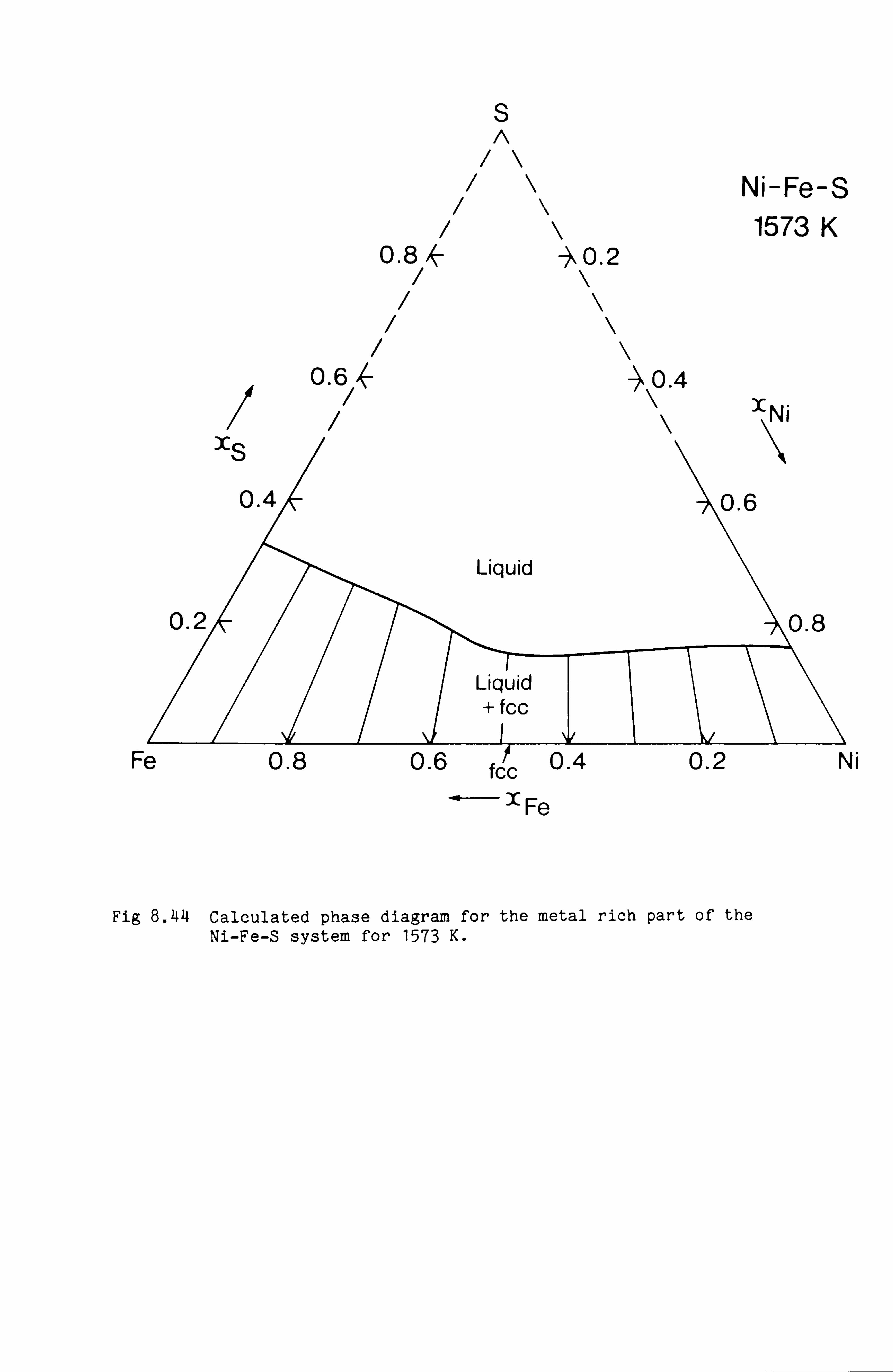
S n
ý Ni-Fe-S 1573 K
0.8 k -ý 0.2
0.64- 0.4
//\\ ýNi
Fe
gx Fe
Ni
Fig 8.44 Calculated phase diagram for the metal rich part of the Ni-Fe-S system for 1573 K.
%. " . %. j %.. 0 . %a fcc W. T %., r . &-

S n
ý Ni-Fe-S 1473 K
0 .80.2
0.6 ý ý. 0.4 ý\ XNi
Fe
~XFe
Ni
Fig 8.45 Calculated phase diagram for the metal rich part of the Ni-Fe-S system for 1473 K.
%. 0 . %. j %. # - %. 4 tcc %. f . --r %. f . ß_

S A
/\
0.8 k -ý 0.2
0.6 0.4
S-
-2.0_ ----
-2.5
0.2
Ni-Fe-S 1473 K
XNi
0.6
o. s -2.75 -2.85
1 -2.8 \ -2.9
Fe 0.8 0.6 0.4 0.2
'-1Fe
Fig 8.46 Calculated phase diagram for the metal rich part of the Ni-Fe-S system for 1473 K with contours for constant sulphur activity expressed as log(pS )/2.
2
Ni

- 111 -
pieces of information were sufficient to define the thermodynamic data
for the monosulphide solid solution phase over the temperature range of
interest. The solid solution in the monsulphide has also been studied by
Kao (517) for 973 K. The calculated phase diagram for 1273 K and 1173 K
are shown in Figures 8.47 and 8.48.
In the Ni-S binary system the beta phase is stable only below 1073 K.
According to Hsieh et al. (499) the beta phase is stable in the ternary
system at 1123 K with the mole fraction of Fe of about 0.2. These
results were not available when this work was carried out and therefore
they have not been considered. Data were developed to represent the
intrusion of the Ni3S2 solid solution phase into the ternary system
based upon the experimental diagram in Craig and Scott (402).
The other phase of interest in this system is the pentlandite phase
(Fe, Ni)9S8 which, according to Kullerud (502) is stable below 883 K.
Data were derived for this phase to be consistent with this observation
and to reproduce the extent of stability of this phase at 673 K shown by
Craig et al. (507). Figures 8.49 and 8.50 shows the region of stability
of pentlandite and its predicted phase relationships for 850 K and 673 K
respectively.
Calculations in the Ni-Fe-Cu-S system
In the quaternary system experimental data are available for the
partial pressure of sulphur above the matte as a function of sulphur
concentration for certain relative proportions of Cu, Fe and Ni
(380,526). Calculations were made using the data derived for the binary
and ternary systems to compare the experimental and predicted
thermodynamic thermodynamic data for the liquid phase. As is shown in
Figures 8.51-8.53 the agreement is excellent even although no new data

S n
/\ Ni-Fe-S 1273 K
0.8 k 30.2 /\
/\ /\
0.6 ýº 0.4 Jý / Pyrrhotite \Y,
�
Fe
'XFe
Ni
Fig 8.47 Calculated phase diagram for the metal rich part of the Ni-Fe-S system for 1273 K.
%J . ki %. / . %J fcc w. -, r W. ̀
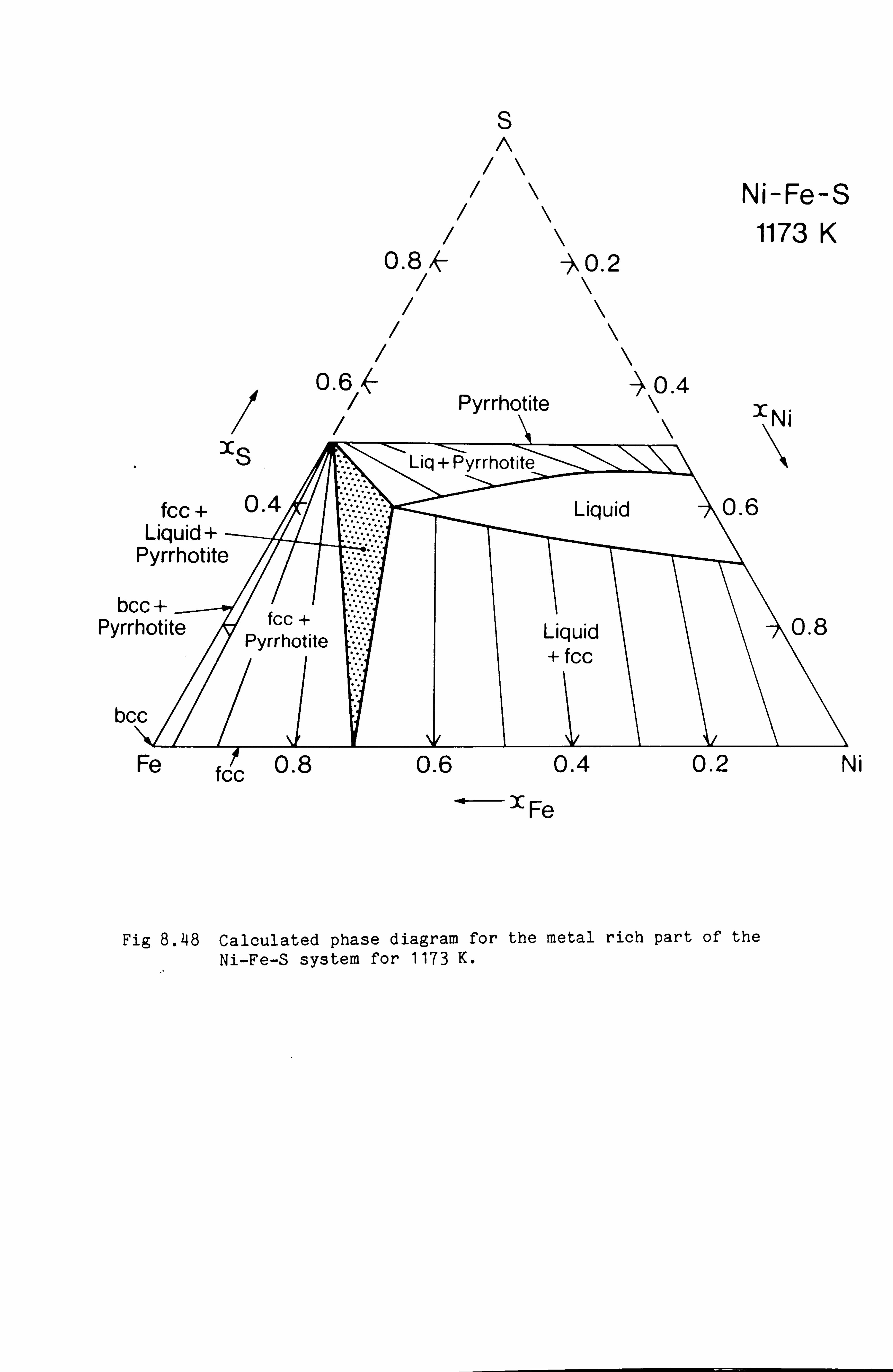
xs
fcc+ 0.4 Liquid+
Pyrrhotite
bcc+_ Pyrrhotite
bcc
Fe fcc
S A
/\ /\
/\ /\
0.8 X 0.2 /\
/\ /\
/\ 0.6 40.4
Pyrrhotite
Liq Pyrrhotite
Liquid
fcc + Pyrrhotite Liquid
0.8
Il II i°° 0.6 0.4
~XFe
Ni-Fe-S 1173 K
xNi
0.6
0.2
0.8
Ni
Fig 8.48 Calculated phase diagram for the metal rich part of the Ni-Fe-S system for 1173 K.
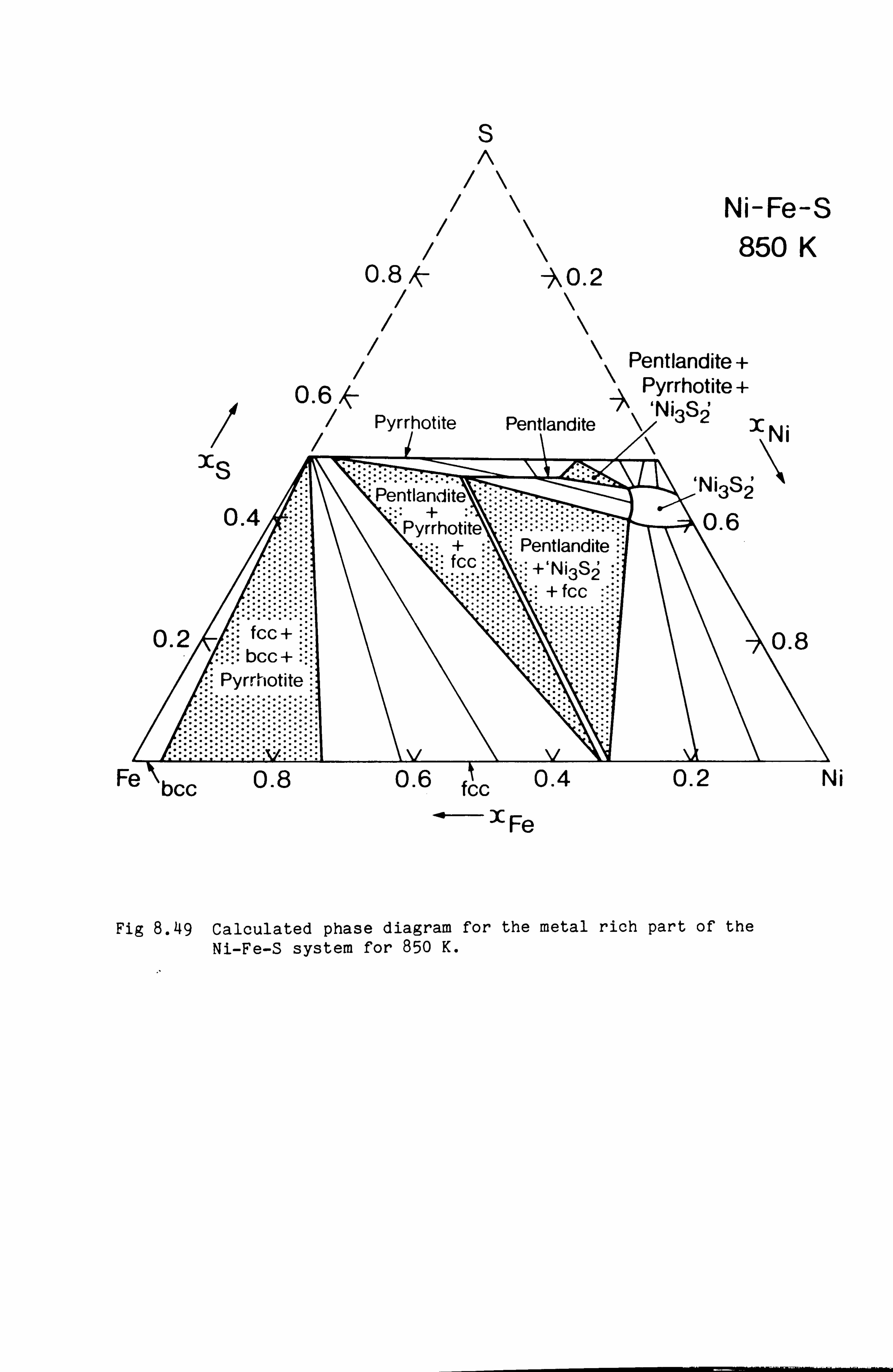
xS
S A
/\ /\
/\ 0.8 A X0.2
0.6, - -ý, Pyrrhotite Pentlandite /11,
0.4
0.2 fcc+ bcc +
Pyrrhotite
Fe\bcc 0.8
Pentlandite +.
Pyrrhotite + Pentlandite fcc :: +`Ni3S2
+ fcc
0.6 fcc 0.4
X Fe
Ni-Fe-S 850 K
Pentlandite + Pyrrhotite + ýNi3S2
x Ni
`Ni3S2
0.6
0.8
0.2 Ni
Fig 8.49 Calculated phase diagram for the metal rich part of the Ni-Fe-S system for 850 K.

0.8ý-
S n
\.
X0.2
Ni-Fe-S 673 K
Pentlandite+ Pyrrhotite+
Pyrrhotite \ Ni7S6
N'
\N i
PentI Bite 0.4
..... + Pentlandite
0.6
Y l'Tý
Pyrrhotite
fcc
0.2 Pyrrhotite
+ fcc + bcc
Fe bcc 0.8 fcc + Pyrrhotite
Ni7S6 `Ni3S2' Heazlewoodite
Pentlandite +`Ni3S2'
. +fcc
0.8
0.4 fcc 0.2
x Fe
Ni
Fig 8.50 Calculated phase diagram for the metal rich part of the
Ni-Fe-S system for 673 K.
- 112 -
were included specifically for the quaternary system.
Fig 8.51 compares the calculated properties with the measured
properties of Bale (526) for 1473 K for different relative proportions
of iron and nickel but with a constant ratio of nickel to copper mole
fractions. Figs 8.52-8.53 compares the calculated properties with those
from Lee (380) for various temperatures and relative mole fraction
ratios of Fe, Ni and Cu.
Conclusions
A new model has been developed for representing the thermodynamic
data for the liquid phase in sulphide systems based upon a two
sublattice model. The model has been tested out and shown to give
results in very good agreement with experimental information.
Data have been derived for all the phases of importance for the metal
rich part of the Cu-Fe-Ni-S system. These are of importance in
understanding and improving processes for the extraction of metals from
ores based on this system. Binary data sets for the Cu-S and Ni-S
systems were critically assessed and combined with data for the Fe-S
system from Fernandez Guillermet et al. and the Cu-Fe-Ni system of Chart
et al. to predict phase equilibria in the ternary and quaternary
systems. Ternary interaction data were derived where appropriate from
any experimental ternary information available. The agreement between
calculated and the experimental phase diagrams and thermodynamic data is
very good especially at lower temperatures. At higher temperatures the
agreement could be improved through a reassessment of the data for a)
the Cu-Fe system taking available ternary data into account, b)the beta
phase with a two sublattice model incorporating the most recent
experimental data and c) the liquid phase with a different notional
charge for nickel ions.

as aýo
" mom xo o ooh
0 13
+
u_ .0 H E +O U a X 0 0 LO ± Ci
CY) cy)
co C\l
LO
U') LO
LO 0 CZ
N qq II
ý. iýt Or" C7 C)
O LO
co co T- ao
O O
Ü a
210
r H O6 O O Ö O T UHk
0 Ö LO o Un dTT
(a/Sd) 6oß
0 LO Ö
0 qt ö S.
Cid
c L
te a) a) . W
r-I ý aý cd cý as
O N L O e cd S.
O "rl > 4-ý
C') U L cd
O LI 0) o b CU r1 Z 4-) ca S U) . >, c Cl)
a) e ý v) "ý cd I L r-I :3 CD a U a O I >C
r1 N W co C14 U 1 "
"r-I ýC c z N rn
o 3
, -) , -
O 0 (1) Cl)
"r4 L C L O cý (1) r4 El) 4-) U U O S. (1)
U d Cl)
LC)
O °0 T 114
oL o0 NN C1) 11

-1. u
1473 K
xFe x T XFe+XNi
-1.5 T Symbol Ox
0.3097 + 0.5803 00
X 0.8155 X
-2.0 xNi
=3.0007 + xCu
-2.5
-3.0 0.30 0.35 0.40 0.45 0.50
xs
-1.5
N -2.0
-2.5
-3.0
-i u
-1.5
E -2.0
xNi =03343 =Cu +
-2.5
-3.0 030 035 040 045 050 xs-
0.30 0.35 0.40 0 45 0.50 Is--- .
Fig 8.52 Comparison between calculated and experimental sulphur pressures in the Ni-Fe-Cu-S system for various pseudo-binary sections for 1673 K and 1706 K. Experimental data from Lee.
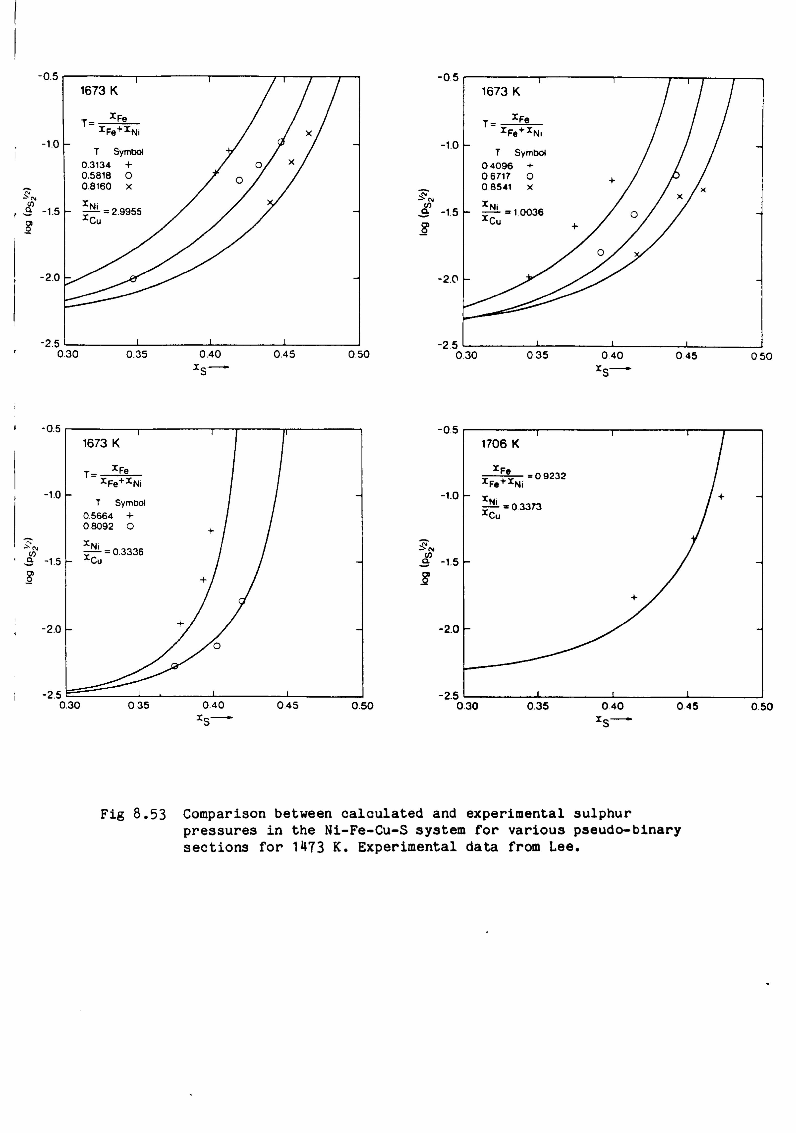
-0.5
-1.0
tV y
-1.5
-2.0
-2.5
1673 K
XFe T__
XFe+XNi x
T Symbol
0.3134 +Ox 0.5818 00 0.8160 x
XNi = 2.9955
xcu
0.30 0.35 0.40 0.45 0.50 xs
' -V. J
-1. o
1 Z'�, Co
v -1.5
-2.0
-25
1673 K
XFe T__ XFe+XNi
T Symbol 0.5664 + 0.8092 0
xN = 0.3336
- Xcu
0.30 0.35 0.40 0.45 0.50 xS--
-0.5
-1.0
N
n -1.5
-2.0
1673 K
_ xFe T
XFe+xNi
T Symbol 04096 + 06717 0
jo
08541 x-
xi =1.0036 xCu
-2.5 11111 0.30 035 040 045 050
xS-
-0.5
-1.0
9 -1.5
-2.0
-2.5
1706 K
XFe =0 9232
XFe+XNi
XNi +
xC= 0.3373
u
0.30 0.35 040 0.45 0.50
Fig 8.53 Comparison between calculated and experimental sulphur pressures in the Ni-Fe-Cu-S system for various pseudo-binary sections for 1473 K. Experimental data from Lee.
- 113 -
CHAPTER 9
Conclusions and Suggestions for Future Work
A wide range of topics have been dealt with in this thesis ranging
from the measurement of the enthalpies of formation for selected alloys
in the Fe-Ti system, the critical assessment of data, development of
models and expressions to represent data, development of procedures for
the calculation of phase diagrams and their use in the calculation of
equilibria for steel and sulphide systems.
A fair degree of success has been achieved in this work although it
must be admitted that in each of these areas more work needs to be done
as has been referred to many times within the text. In particular this
thesis has highlighted the need for more theoretical work to understand
and represent the various contributions which comprise thermodynamic
data. For elements the liquid phase is not well understood and in
particular the structural changes leading to the glass transition which
occurs as a liquid is cooled down usually below its freezing point. For
phase diagram calculations data are also required for elements in
unstable phase structures. Theoretical work to provide such data would
be most welcome.
For binary systems many reliable models are now available to
represent the data for solid phases. Unfortunately the correct choice of
models will depend particularly on the structural characteristics of the
material and how these change as the composition or temperature is
varied. In this thesis two solid 'compound' phases were of particular
importance - the Laves phase compound Fe2Ti and the phase or phases
based about Ni3S2. The former exists over a wide range of homogeneity in
the binary system and although its structure (C14) is known, the way the
occupation of lattice sites changes with composition is not. The

- 114 -
situation is worse for Ni3S2 since it seems to be virtually unquenchable
and its structure is not known at all. Furthermore not only does it
exist over a wide range of homogeneity in the Ni-S binary system but it
also dissolves significant quantities of Cu and Fe. To complete the
gloomy picture there is evidence to suggest that the phase is not just
one phase but two phases. In this thesis data for Ni3S2 and Fe2Ti were
represented by a Redlich-Kister power series expression which was a
convenient although not necessarily physically correct description. Both
these phases should be reconsidered using structural models once the
required experimental structural information is available.
For multicomponent systems much work still need to be done to develop
and test out models to represent thermodynamic data. The work reported
here on sulphide systems and in particular the liquid phase was very
successful although improvements could be made in the representation of
the data for the Cu-Ni-S system. In particular the use of a different
notional valency for nickel would be of great interest. This would
require a reassessment of the Ni-S binary system which could be carried
out in conjunction with a revised treatment of Ni3S2,
More recently Hillert et al. have suggested a new model for liquid
phases based upon a sublattice description. This model seems more
general and versatile than that used in the present work and it is hoped
that it will soon be tested out on sulphide systems. Also of great
importance is the development of reliable but versatile models for oxide
systems and in particular slags.
In more general terms there needs to be continued development of
systems for the calculation of phase equilibria linked to databases for
the use of industry. This requires a long term programme of data
assessment work, backed up by basic experimental work, to create a self
consistent database and the development of sophisticated software to
simulate industrial processes. Effort must also be made to encourage

- 115 -
industry to use such facilities.
The work reported in this thesis is only a small part in a worldwide
effort in thermodynamics but it is to be hoped that it has made some
contribution to the generation and application of chemical and
metallurgical thermodynamic data.
ACKNOWLEDGEMENTS
There are many people who have helped me in this work over the last few
years but I would like to mention a few to whom I owe special thanks:
- Prof. C. Bodsworth for his advice and great patience throughout this
project,
- Dr T. G. Chart for his continuous support, interest and valuable
contributions,
- My colleagues within MTDS, Dr T. I. Barry, Mrs F. H. Putland, R. H.
Davies, Dr M. H. Rand, D. D. Gohil, Mrs S. Hodson and M. Dunlop for
many lively discussions, assistance and suggestions for improving my
work,
- Dr C. W. Bale for making available his experimental work on sulphide
systems,
- Dr J. R. Taylor and Johnson Matthey Limited for their permission to
include my work on sulphide systems within this thesis,
- My family and especially my wife, Alison, who have been a constant
source of inspiration. Alison in particular has shown great strength
and patience over the last two years through various trials and
while our house and garden were neglected in the interests of
metallurgical thermodynamics.
Alan Dinsdale 20 August 1984

- Al -
APPENDIX
The liquid phase is chosen as the reference phase for each of the elements. T
parameters for the Gibbs energies of formation for the various phases
interest in J mol-1 are:
Liquid
°GNi =0
G Fe =0
°GCu =0
°Gs =0
0 GNiS = -71390.17 - 7.45917 T 0 GFeS -80947 - 129.155 T-0.0041755 T2 + 16.291 T ln(T)
°GCu s= -86094 - 22.291 T
2 G[Ni: S, Vc] _ (-67995.65 + 21.1647 T)
+ (-51984.49 + 17.0106 T) (ZS-ZVc)
+ (-1193.338 + 3.55053 T) (ZS-Zvc)2
G[Fe: S, Vc] _ (31761 - 9.202 T)
+ (40761 - 0.477 T) (ZS-ZVc)
G[Cu: S, Vc] (19385 + 17.076 T)
+ (-3718 - 0.879 T) (ZS - Zve)
G[Va: S, Vc] = 100 T
G[Ni, Fe: S] -10035.03
G[Ni, Cu: S] = 15000 + 10000 (ZNi - ZCu)
G[Ni, Va: S] ( 23228.52 - 2.8569 T)
+ (-10168.80 - 9.5614 T) (ZNi-ZVa)
G[ Fe, Cu : S] =0
G[Fe, Va: S] (79779 - 45.139 T)
+ (-57510 + 17.082 T) (ZFe-ZVa)
I

- A2 -
G[Cu, Va: S] _ (107706 + 21.338 T)
+ (-6011 - 3.514 T) (ZCu-ZVa)
+ (-39812 - 5.424 T) (ZCu-ZVa)2
G[Ni, Fe: Vc] = (-20292.4 + 5.9622 T)
+ (-11924.4 + 3.2426 T) (ZNi_ZFe)
G[Ni, Cu: Vc] _ (10460 + 2.0878 T)
+ (1451.8 - 0.3933 T) (ZNi-ZCu)
G[Ni, Va: Vc] = 100 T
G[Fe, Cu: Vc] _ (34321.3 - 1.8577 T)
+ (1811.6 - 1.6401 T) (ZFe-ZCu)
+ (7564.6 - 2.5857 T) (ZFe-ZCu)2
+ (2418.3 - 2.3472 T) (ZFe-ZCu) 3
G[Fe, Va: Vc] = 100 T
G[Cu, Va: Vc] = 100 T
G[Ni, Fe: S, Vc] = 20136.96 + 9913.78 (ZNi - ZFe) - 13519.09 (ZS - ZVc)
G[Ni, Cu: S, Vc] _ -25000 + 20000 (ZS - ZVc)
G[Fe, Cu: S, Vc] =0
fcc
0GNi -17614.6 + 10.209 T
0 GFe- = 11274 - 163.878 T-0.0041756 T2 + 22.03 T ln(T)
0GCu = -13054.1 + 9.6232 T
G[Ni, Fe] (-16359.4 + 1.02872E-2 T2 - 4.384E-6 T3)
+ (-18451.4 + 1.41177E-2 T2 - 6.017E-6 T3) (x -xFe)
G[Ni, Cu] _ (8137.8 + 3.0083 T)
+ (2535.5 - 0.8284 T) (xNi-xCu)
G[Fe, Cu] (48208.0 - 8.4475 T)
+ (5916.1 - 5.0166 T) (XFe-XCu)
G[Ni, Fe, Cu] = -62760 + 20.5 T

_A3_
bcc
0 GNi = -31106.99 + 102.0017 T-9.9718E-3 T2
+ 3.192592E-6 T3 - 10.06475 T ln(T) + 2693466.3 T-1
°GFe = -268257. ' + 2388... 3802 T+0.1867633 T2
- 18.26149E-6 T3 - 337.18251 T ln(T) + 35590150 T-1
°GCu = -6778.0 + 6.276 T
G[Ni, Fe] _ (-7'468.4 + 1.83699E-2 T2 - 7.3894E-6 T3)
+ (-8807.3 + 1.701423E-2 T2 - 5.8024E-6 T3) (xNi-xFe)
G[Ni, Cu] _ (8137.8 + 3.0083 T)
+ (2535.5 - 0.8284 T) (xNi-xCu)
G[Fe, Cu] _ (10890.9 + 88.1276 T-6.15885E-2 T2
+ 1.2857E-5 T3)
+ (2071.0 - 10.6357 T) (xFe-xCu)
G[Ni, Fe, Cu] =0
L-4
eGNi = -17614.6 + 10.209 T
0GFe = 11274 - 163.878 T-0.0041756 T2 + 22.03 T in(T)
G[Ni, Fe] (-30965.7 + 29.6604 T)
+ (-26087.2) (xNi-xFe)_
+( 297.0) (xNi-xFe)2
+( 18468.1) (xNi-xFe)3

- Au -
Beta
0 GNi 290443.6412 - 167.5003 T
°GFe = 290443.6412 - 167.5003 T
0 GCu = 290443.6412 - 167.5003 T
0G5 = 65357 - 165.396 T+ 13.513 T ln(T)
G[Ni, Fe] =0
G[Ni, Cu] =0
G[Ni, S] _ (-896377.028 + 515.2259 T)
+ (-560488.9k2 + 206.182 T) (xNi-xS)
G[Fe, Cu] =0
G[Fe, S] _ -551900 + 300 T
G[Cu, S] -902000 + 666.7 T
G[Ni, Fe, Cu] =0
G[Ni, Fe, S] _ -1655700 + 900 T
G[Ni, Cu, S] _ -600000
G[Fe, Cu, S] =0
Gas
G[1S2] 65357 - 165.396 T+ 13.513 T in(T) 2
Pyrrhotite
oGNiS = -157743.33 + 375.2205 T- 44.372 T ln(T)
0GFeS = -93486 - 127.434 T+ 16.358 T ln(T)
GCu2S = -75000 - 120.321 + 13.513 T
G[Ni, Fe: S] = 18192.03 - 15.12 T
G[Ni, Cu: S] = 30000
G[Fe, Cu: S] =0

- A5 -
Digenite
°GNiS = -60000 - 130 T+ 16.358 T ln(T)
° GFeS = -84400 - 130 T+ 16.358 T ln(T)
°GCu s -86136 - 120.321 T+ 13.513 T ln(T)
2 G[Ni, Fe: S] =0
G[Ni, Cu: S] = 50000
G[Cu, Fe: S] =0
Chalcocite
0GCu 2S
- -87969 - 117.732 T+ 13.513 T ln(T)
0 Gc s= -44220 - 103.674 T+ 13.513 T ln(T)
Millerite
ýGNiS = -125300.00 - 49.64 T+ 13.513 T ln(T)
Heazlewoodite
ýGNi
3S= -235901.51 + 21.5438 T
2
Ni
ýGNi 7s6=
1559472.551 - 23670.842 T+ 3133.897 T in(T)

- A6 -
Pentlandite
0GNi 9S8=
-937626.3 + 195.48 T
OGFe S= -655929.018 - 1352.3247 T+ 178.3323 T ln(T)
98 G[Ni, Fe: S] (-918799.002 + 809.523 T)
+ (-326892.6 + 485.7138 T) (ZNi - ZFe)

- R1 -
References
1. Gibbs J. W., Trans. Conn. Acad. Sci., 1876,39 228
2. Clausius R. J. E., "The Mechanical Theory of Heat", transl. Hirst,
1867
3. Planck M., Ann. Physik, 1901,14,553
ü. Planck M., "Treatise of Thermodynamics", transl. Ogg, 1927
5. Boltzmann L., "Vorlesungen uber Gastheorie", Johann Ambrosius
Barth Verlag, Leipzig, 1912
6. Nernst W., Nachr. kgl. Ges. Wiss. Gottingen Math. -physik. kl.,
1906,1
7. "The Physical Chemistry of Metallic Solutions and Intermetallic
Compounds", National Physical Laboratory Symposium No 9, HMSO,
1959
8. "Metallurgical Thermochemistry", Proc. Symp. Brunel Univ. and
National Physical Laboratory, HMSO, 1972, ed. O. Kubaschewski
9. "Fluids and Fluid Mixtures", Proc. Conf., National Physical
Laboratory, Publ. IPC Science and Technology Press, 1978
10. "The Industrial Use of Thermochemical Data", Proc. Conf., ed.
T. I. Barry, Publ. The Chemical Society, Sept 11-13,1979
11. Potter P. E., Rand P. H. , ibid, p149
12. Edwards J., Potter P. E., ibid, p160
13. Carlson O. N., Chiotti P., Shiers L., ibid, p169
14. Kaufman L., ibid, p215
15. Chart T. G., Dinsdale A. T., Putland F. H., ibid, p235
16. Burkin A. R., ibid, p180
17. Teyssandier F., Ducarrior M., Bernard C., ibid, p301
18. Glasson D. R., O'Neill P., ibid, p118
19. Hoch M., Chen Y. S., ibid, p312
Franz-Stern R., Stern I., Bogdanic G., ibid, P325

-R2-
21. Olette M., Steiler J. M., ibid, P368
22. Steiler J. M., Capelani R., ibid, p391
23. Kyle J., ibid, p403
24. Work D. E., ibid, p128
25. Mottram D. A. J., ibid, p139
26. Dench W. A., Trans. Faraday Soc., 1963,59,1279
27. Stull D. R., Prophet H., "JANAF Thermochemical Tables", US
Department of Commerce, Washington, 1971
28. Chase M. W., et al., J. Phys. Chem. Ref. Dat., 1974,3,311
29. Chase M. W., et al., ibid, 1975,4,1
30. Chase M. W., et al., ibid, 1978,7,793
31. Chase M. W., et al., ibid, 1982,11,695
32. Barin I., Knacke 0., "Thermochemical Properties of Inorganic
Substances", S pringer-Verlag, Berlin 1973
33. Barin I., Knacke 0., Kubaschewski 0., Supplement to Ref. 32,1977
34. Gurvich L. V., Veits I. V., Medved'ev V. A., Khachkuruzov G. A.,
Yungman V. S., Bergman G. A., ed. V. P. Glushko, "Thermodynamic
Properties of Individual Substances", Vol 1, Izd. Nauka, Moscow,
1978
35. Gurvich L. V., Veits I. V., Medved'ev V. A., Khachkuruzov G. A.,
Yungman V. S., Bergman G. A., ed. V. P. Glushko, "Thermodynamic
Properties of Individual Substances", Vol 2, Izd. Nauka, Moscow,
1979
36. Gurvich L. V., Veits I. V., Medved'ev V. A., Khachkuruzov G. A.,
Yungman V. S., Bergman G. A., ed. V. P. Glushko, "Thermodynamic
Properties of Individual Substances", Vol 3, Izd. Nauka, Moscow,
1981
37. Gurvich L. V., Veits I. V., Medved'ev V. A., Khachkuruzov G. A.,
Yungman V. S., Bergman G. A., ed. V. P. Glushko, "Thermodynamic
Properties of Individual Substances", Vol 4, Izd. Nauka, Moscow,
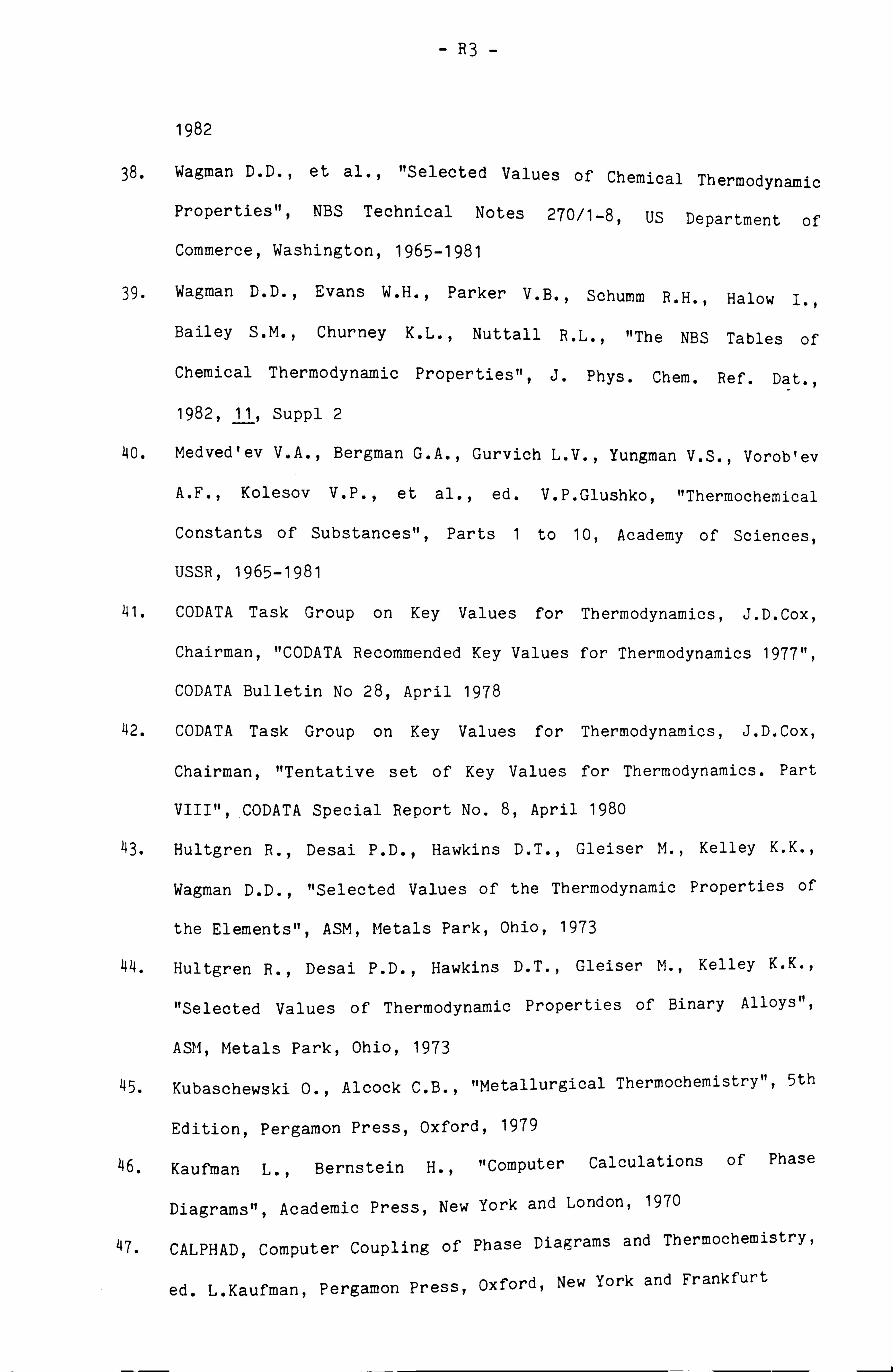
- R3 -
1982
38. Wagman D. D., et al., "Selected Values of Chemical Thermodynamic
Properties", NBS Technical Notes 270/1-8, US Department of
Commerce, Washington, 1965-1981
39. Wagman D. D., Evans W. H., Parker V. B., Schumm R. H., Halow I.,
Bailey S. M., Churney K. L., Nuttall R. L., "The NBS Tables of
Chemical Thermodynamic Properties", J. Phys. Chem. Ref. Dat.,
1982,11, Suppl 2
40. Medved'ev V. A., Bergman G. A., Gurvich L. V., Yungman V. S., Vorob'ev
A. F., Kolesov V. P., et al., ed. V. P. Glushko, "Thermochemical
Constants of Substances", Parts 1 to 10, Academy of Sciences,
USSR, 1965-1981
41. CODATA Task Group on Key Values for Thermodynamics, J. D. Cox,
Chairman, "CODATA Recommended Key Values for Thermodynamics 1977",
CODATA Bulletin No 28, April 1978
42. CODATA Task Group on Key Values for Thermodynamics, J. D. Cox,
Chairman, "Tentative set of Key Values for Thermodynamics. Part
VIII"9 CODATA Special Report No. 8, April 1980
43. Hultgren R., Desai P. D., Hawkins D. T., Gleiser M., Kelley K. K.,
Wagman D. D., "Selected Values of the Thermodynamic Properties of
the Elements", ASM, Metals Park, Ohio, 1973
44. Hultgren R., Desai P. D., Hawkins D. T., Gleiser M., Kelley K. K.,
"Selected Values of Thermodynamic Properties of Binary Alloys",
ASM, Metals Park, Ohio, 1973
45. Kubaschewski 0., Alcock C. B., "Metallurgical Thermochemistry", 5th
Edition, Pergamon Press, Oxford, 1979
46. Kaufman L., Bernstein H., "Computer Calculations of Phase
Diagrams", Academic Press, New York and London, 1970
47. CALPHAD, Computer Coupling of Phase Diagrams and Thermochemistry,
ed. L. Kaufman, Pergamon Press, Oxford, New York and Frankfurt

- R4 -
48. Chipman J., J. Iron Steel Inst., 1955,180,97
49. Elliott J. F., Gleiser M., Ramakrishna V., "Thermodynamics for
Steelmaking II", p491,1963, Reading, Mass., USA, (Addison-Wesley)
50. Schenck H., Steinmetz E., Supplemental Edition of Stahleisen - Sonderberichte, 1968,7,1
51. Sigworth G. K., Elliott J. F., Can. Met. Quart., 1974,13,455
52. Sigworth G. K., Elliott J. F., Metal Sci., 1974,8,298
53. Hansen M., Anderko K., "Constitution of Binary Alloys",
McGraw-Hill, New York, 1958
54. Elliott R. P., "Constitution of Binary Alloys", First Supplement,
McGraw-Hill, New York, 1965
55. Shunk F. A., "Constitution of Binary Alloys", Second Supplement,
McGraw-Hill, New York, 1969
56. Moffatt W. G., "Handbook of Binary Phase Diagrams", General
Electric, New York, Vols 1-3 and supplements, 1976
57. Prince A., "Multicomponent Alloy Constitution Bibliography
1955-1973", The Metals Society, London, 1978
58. Prince A., "Multicomponent Alloy Constitution Bibliography
1974-1977", The Metals Society, London, 1981
59. Ageev N. V., "Diagrammy Sostoyaniya Metallichestikh Sistem", Nos.
1-26, Viniti, Moscow, 1959-1982
60. Wisniak J., "Phase Diagrams", Parts A and B, Elsevier, Amsterdam,
Oxford and New York, 1981
61. Pourbaix M., "Atlas of Electrochemical Equilibria in Aqueous
Solutions", Pergammon Press, Oxford, 1966
62. Levin E. M., Robbins C. R., McMurdie H. F., "Phase Diagrams for
Ceramicists", Amer. Ceramic Soc., Columbus, 1964, Supplements 1969
and 1975
63. "Metals Handbook", 8th Ed., Vol. 8, Metallography, Structure and
Phase Diagrams, American Society for Metals, Metals Park, Ohio,

- R5 -
1973
64. Bulletin of Alloy Phase Diagrams, ed. Bennett L. H., ASM
65. Hillert M., "Prediction of Iron-Base Phase Diagram", Report TRITA-MAC-0132, Stockholm, 1977
66. Henig E. -Th, Lukas H. L., Petzow G., Contemporary Inorganic
Materials, 1978, S1
67. Pelton A. D., Thompson W. T., Progress Solid State Chem., 1975,10,
119
68. Rivlin V. G., Raynor G. V., Int. Metall. Rev., 1980,25,21; 79;
139; 1981,26,133
69. Raynor G. V., Rivlin V. G., Int. Metall. Rev., 1981,26,213
70. Rivlin V. G., Int. Metall. Rev., 1981,26,269
71. Raynor G. V., Rivlin V. G., Int. Metall. Rev., 1982,27,169; 289;
1983,28,23; 122; 211; 251
72. Rivlin V. G., Int. Metall. Rev., 1983,28,309; 1984,29,96
73. Chang Y. A., N eumann J. P., Mikula A., Goldberg D., "Phase Diagrams
and Thermodynamic Properties of Ternary Copper-Metal Systems",
INCRA Monograph VI, The Metallurgy of Copper, 1979
74. Chang Y. A., Neumann J. P., Choudary U. V., "Phase Diagrams and
Thermodynamic Properties of Ternary Copper-Sulfur-Metal Systems",
INCRA Monograph VII, The Metallurgy of Copper, 1979
75. Inden G., Proceedings CALPHAD Conference, Dusseldorf, 1976, III,
4-1.
76. Inden G., Physica, 1981,103B, 82.
77. Hillert M., Jarl M., CALPHAD, 1978,2,227.
78. Oriani R. A., Alcock C. B., Trans. Metall. Soc. AIME., 1962,224,
1104.
79. Ansara I., Int. Metall. Rev., 1979,249 20.
80. Ansara I., in 'Metallurgical Chemistry', Proc. Symp. Brunel
Univ. -NPL, 1971.

- R6 -
81. Kapoor M. L., Int. Metall. Rev., 1975,20,150.
82, Hildebrand J. H., Proc. Nat. Acad. Sci., 1927,139 267.
83. Hildebrand J. H., J. Amer. Chem. Soc., 1929,519 66.
$4, Hildebrand J. H., Scott R. L., "The Solubility of Non-Electrolytes",
3rd ed (New York, Rheinhold, 1950).
85. Heitler W., Ann. Physik, 1926,80,629
86. Herzfeld K. F., Heitler W., Zeit: fur Electrochem., 1925,31,536.
87. Bragg W. L., Williams E. J., Proc. Roy. Soc., 1934, A145,699.
88. Meijering J. L., Acta Met., 1957,5,527.
89. Hurle, D. T. J., Pike E. R., J. Mater. Sei, 1966,1,399.
90. Lehovec K, Slobodskoy A, J. Electrochem. Soc., 1964 , 111,65.
91. Guggenheim E. A., Proc. Roy. Soc. (London), 1935, A148,304.
92. Rushbrooke G. S., Proc. Roy. Soc. (London), 1938, A166,296.
93. Guggenheim E. A., 'Mixtures', 1952, Oxford University Press.
94. Fowler R. H., Proc. Camb. Phil. Soc., 1938,34,382.
95. Fowler R. H., Guggenheim E. A., 'Statistical thermodynamics', 1960,
Cambridge University Press.
96. Bethe H., Proc. Roy. Soc., 1935, A150,552.
97. Bonnier E., Durand F., Laurent P-J., C. R. Hebd. Seances Acad.
Sci., 1962,254,107.
98. Jena A. K., Metall. Trans., 1970, 1, 1260.
99. Stringfellow G. B., Greene P. E., J. Phys. Chem. Solids, 1969,30,
1779.
100. Stringfellow G. B., Greene P. E., J. Electrochem. Soc., Solid State
Sci., 1970,117,1075.
101. Kleppa O. J., J. Amer. Ch em. Soc., 1950,72,3346.
102. Hagemark K. I., J. Chem. Phys., 1973,59,2344.
103. Hagemark K. I., J. Chem. Phys., 1974,61,2596.
104. Wagner C., Acta Metall., 1973, 21,1297.
105. Li Y. Y., J. Chem. Phys., 1949, 17,1447.

-R7-
106. Takagi Y., Proc. Phys. Math. Soc. Japan 1941,239 44.
107. Kikuchi R., Phys. Rev., 1951,81,988.
108. Kurata M., Kikuchi R., J. Chem. Phys., 1953, 21, 434.
109. Kikuchi R., Brush S. G., J. Chem. Phys., 1967, 47, 195.
110. Kikuchi R., J. Chem. Phys., 1974,60,1071.
111. Kikuchi R., Acta Metall., 1977,25,195.
112. Kikuchi R., de Fontaine D., Murakami M., Nakamura T., Acta
Metall., 1977,25,207.
113. Kikuchi R., J. de Phys., 1977,38, C7-307-
114. Kikuchi R., Physica, 1981,103B, 41.
115. Kikuchi R., CALPHAD, 1982,6 , 1.
116. van Baal C. M., Physica 1973,64,571.
117. Hume-Rothery W., Mabbott G. W., Channel-Evans K. M., Phil. Trans.
Roy. Soc. (London), 1934, A233,1.
118. Buckley R. A., Hume-Rothery W., J. Iron Steel Inst (London), 1963,
201,227.
119. Hume-Rothery W., "Phase Stability in Metals and Alloys", (P. S.
Rudman, J. Stringer, and R. I. Jaffe eds) McGraw Hill, New York
1967.
120. Hardy H. K., Acta Met., 1953,1,202.
121. Sharkey R. L., Pool M. J., Hoch M., Metall. Trans., 1971,2,3039.
122. Lupis C. H. P., Elliott J. F., Acta Metall., 1967, 15,265.
123. Mathieu J. C., Durand F., Bonnier E., J. Chim. Phys., 1965,62,
1289.
124. Mathieu J. C., Durand F., Bonnier E., J. Chim. Phys., 1965,629
1297.
125. Hicter P., Mathieu J. C., Durand F., Bonnier E., J. Chim. Phys.,
1967,64,261.
126. Brion B., Mathieu J. C., Hicter P., Desre P., J. Chim. Phys., 1969,
66,1238.
-R8-
127. Brion B., Mathieu J. C., Hicter P., Desre P., J. Chim. Phys., 1970,
67,1745.
128. Margules M., Akad. Wiss. Wien, Sitzungs., Math. -Naturwiss., 1895,
104,12143.
129. Zawidzki J. von, Z. Phys. Chem., 1909,69,630.
130. Guggenheim E. A., Trans Faraday Soc., 1937,33,151.
131. Wohl K., Trans. Amer. Inst. Chem. Eng., 1946,62,215.
132. Carlson H. C., Colburn, A. P., Ind. Eng. Chem., 1942,34,581.
133. Benedict M., Johnson C. A., Solomon E., Rubin L. C., Trans. Amer.
Inst. Chem. Eng., 1945,41,371.
134. Bale C. W., Pelton A. D., Can. Met. Quart. 1975,14,213.
135. Bale C. W., Pelton A. D., Metall. Trans., 1974,5,2323.
136. Krupkowski A., Bull. Acad. Polon. Sci. Lett., Ser. A, 1950,1 , 15.
137. Esdaile J. D., Metall. Trans. B, 1982,13B, 213.
138. Wilson G. W., J. Am. Chem. Soc., 1964,86,127.
139. Redlich 0., Kister A. T., Ind. Eng. Chem., 1948,40,345.
140. Redlich 0., Kister A. T., Turnquist C. E., Chem. Eng. Progr. Symp.
Ser., 1952,48,49.
141. Bonnier E., Caboz R., C. R. Hebd. Seances Acad. Sci., 1960, 250,
527.
142. Spencer P. J., Hayes F. H., and Kubaschewski 0., Revue de Chimie
Minerale, 1972 9,13.
143. Toop G. W., Trans. Metall. Soc. AIME, 1965,233,850.
144. Ajersch F., Hayer E., Barbier J-N., Ansara I., Z. Metallkde.,
1975,66,624.
145. Kohler F., Monatsh. Chem., 1960,91,738.
146. Olson N. J., Toop G. W., Trans. AIME., 1966,236,590.
147. Kehiaian H., Bull. Acad. Pol. Sci., 1966,14,153.
148. Kaufman L., Nesor H., Metall. Trans., 1974,5,1617.
149. Kaufman L., Nesor H., Metall. Trans., 1974,5,1623.

- R9 -
150. Kaufman L., Nesor H., Metall. Trans., 1975,6A, 2115.
151. Kaufman L., Nesor H., Metall. Trans., 1975,6A, 2123.
152. Kaufman L., Nesor H., CALPHAD 1978,2,35.
153. Kaufman L., Tanner L. E., CALPHAD, 1979,3,91.
154. Dew-Hug hes D., Kaufman L., CALPHAD, 1979,3,175.
155. Kaufman L., CALPHAD, 1979,3,27.
156. Kaufman L., CALPHAD, 1979,3,275.
157. Kaufman L., Hayes F., Birnie D., CALPHAD, 1981,5,163.
158. Kaufman L., Nell J., Taylor K., Hayes F., CALPHAD, 1981, 5,185.
159. Kaufman L., Agren J., Nell J., Hayes F., CALPHAD, 1983, 7,71.
160. Ansara I., G ambino M., Bros J. P., J. Cryst. Growth 1976, 32,101.
161. Pelton A. D., Bale C. W., CALPHAD 1977,1,253.
162. Darken L. S., J. Amer. Chem. Soc., 1950,72,2909.
163. Colinet C., D. E. S., Fac. Sci. Univ. Grenoble, France, 19 67.
164. Muggianu Y. M., Gambino M., Bros J. P., J. Chim. Phys., 1975,72,
83.
165. Jacobs K. J., Fitzner K., Thermochimica Acta, 1977,18,197.
166. Hillert M., CALPHAD, 1980 , 4,1.
167. Chart T. G., Putland F. H., Dinsdale A. T., CALPHAD, 1980,41 27.
168. Putland F. H. , Chart T. G., Dinsdale A. T., CALPHAD, 1980,1,133.
169. Chart T. G., Gohil D. D., Xing Zhong shu, NPL Report DMA (A) 54,
August 1982.
170. Ansara I., Bernard C., Kaufman L., Spencer P. J., CALPHAD, 1978,2,
1.
171. Ansara I., Bonnier E., Monatshefte fur Chemie 1971,102,1855.
172. Dinsdale A. T., National Physical Laboratory Internal Report, DCS
1/78, February 1978.
173. Dinsdale A. T., National Physical Laboratory Report, Chem 90, July
1978.
174. Throop G. J., Rogl P., Rudy E., High Temperatures - High Pressures,

- R10 -
1978,10,553.
175. Sundman B., Agren J., J. Phys. Chem. Solids, 1981,42,297.
176. Hillert M., Staffansson L. I., Acta Chem. Scand., 1970,24,3618.
177. Harvig H., Acta Chem. Scand., 1971,25,3199.
178. Wagner C., Schottky W., Z. Physik. Chem., 1931, B11,163.
179. Libowitz G. G., Lightstone J. B., J. Phys. Chem. Solids, 1967,28,
1145.
180. Libowitz G. G., J. Solid State Chem., 1969,1,50.
181. Brebrick R. F., J. Solid State Chem., 1969,1,88.
182. Hertzman S., Sundman B., Royal Institute of Technology Report
TRITA-MAC-0180, Stockholm, Jan 1981.
183. Hertzman S., Sundman B., CALPHAD, 1982,6,67.
184. Temkin M., Acta Phys. Chim. USSR, 1945,20,411.
185. Flood H., Forland T., Grjotheim K., Z. Anorg. Chem., 1954,276,
289
186. Forland T., Norg. Tek. Vitenskapsakad, 1957, ser 2, no ü
187. Chart T. G., Unpublished work.
188. Oonk H. A. J., Blok K., van de Koot B., Brouwer N., CALPHAD, 1981,
5,55
189. Bouwstra J. A., Oonk H. A. J., CALPHAD, 1982,6,11
190. Oonk H. A. J., Blok G. J., Bouwstra J. A., CALPHAD, 1983,7,211
191. Saboungi M. -L., Blander M., J. Am. Ceram. Soc., 1974,58,1
192. Saboungi M. -L., Blander M., J. Chem. Phys., 1975,63,212
193. Saboungi M. -L., J. Chem. Phys., 1980,73,5800
194. Bale C. W., Pelton A. D., CALPHAD, 1982,6,255
195. Pelton A. D., Lin P. L., CALPHAD, 1983,7,295
196. Hillert M. , Jansson B. , Sundman B. , Agren J. , Royal Institute of
Technology Report TRITA-MAC-0218 (Revised), Feb 1984.
197. Eliezer N., Howald R. A., Marinkovic M., Eliezer I., J. Phys.
Chem., 1978,82,1021.

- R11 -
198. Eliezer I., Eliezer N., Howald R. A., Verwolf M. C., CALPHAD 1979,
3,1.
199. Byker H. J., Craig R. E. R., Eliezer I., Eliezer N., Howald R. A.,
Viswanadham P., CALPHAD 1981,5,217.
200. Chang D. R., Howald R. A., Roy B. N., CALPHAD 1982,6,83.
201. Eliezer I., Eliezer N., Howald R. A., Viswanadham P., J. Phys.
Chem., 1981,85,2835.
202. Kaestle G., Koch K., Proc. CALPHAD Conference, Stuttgart 1978, p6.
203. Lumsden in "Physical Chemistry of Process Metallurgy", G. R. St
Pierre ed., ppl65-205, Interscience, New York, 1961.
204. Sharma, R. C., Chang Y. A., Metall. Trans., 1980,11B, 575.
205. Dolezalek F., Z. Phys. Chem., 1908,64,727.
206. Lacmann R., Z. Phys. Chem. Neue Folge, 1960,23,313.
207. Lacmann R., Z. Phys. Chem. Neue Folge, 1960,23,324.
208. Lacmann R., Z. Phys. Chem. Neue Folge, 1962,35,86.
209. Jordan A. S., Zupp R. R., J. Electrochem. Soc., 1969,116,1264.
210. Jordan A. S., Metall. Trans., 1970,1,239.
211. Jordan A. S., Metall. Trans., 1976,7B, 191.
212. Gerling U., pool M. J., Predel B., Z. Metallkde., 1983,74,616.
213. Kellogg H. H., Can. Metall. Quart., 1969,8,3.
214. Kellogg H. H., in 'Physical Chemistry in Metallurgy', 1976, eds.
R. M. Fisher, R. A. Oriani, E. T. Turkdogan (Monroeville, PA: US Steel
Research), 49.
215. Predel B., Oehme G., Z. Metallkde., 1976,67,826.
216. Chang Y. A., Sharma R. C., in 'Calculation of Phase Diagrams and
Thermochemistry of Alloy Phases', eds. Y. A. Chang, J. F. Smith, 1979,
(Metals Park, OH: American Society for Metals), 145.
217. Larrain J. M., CALPHAD, 1979,3,139.
218. Larrain J. M., CALPHAD, 1980,49 155.
219. Larrain J. M., Kellogg H. H., in 'Calculation of Phase Diagrams and

- R12 -
Thermochemistry of Alloy Phases', eds. Y. A. Chang, J. F. Smith, 1979,
(Metals Park, OH: American Society for Metals), 130.
220. Larrain J. M., Lee S. L., Kellogg H. H., Can. Metall. Quart., 1979,
18,395.
221. Sharma R. C., Chang Y. A., Metall. Trans., 1979,10B, 103.
222. Sharma R. C., Chang Y. A., Z. Metallkde., 1979,70,104.
223. Sharma R. C., Chang Y. A., Metall. Trans., 1980,11B, 139.
224. Fosnacht D. R., Goel R. P., Larrain J. M., Metall. Trans., 1980,11B,
69.
225. Bhatia A. B., Hargrove W. H., Phys. Rev. B, 1974,10,3186.
226. Osamura K., Nakajima K., Murakami Y., J. Electrochem. Soc., 1979,
126,1992.
227. Sommer F., Predel B., Eschenweck D., Oehme G., Berichte der
Bunsen-Gesellschaft, 1977,81,997.
228. Goel R. P., Kellogg H. H., Larrain J. M., Metall. Trans., 1980,11B,
107.
229. Hillert M., Staffansson L. I., Metall. Trans., 1975,6B, 37.
230. Staff ansson L. I., Metall. Trans., 1976,7B, 131.
231. Hillert M., Staffansson L. I., Metall. Trans., 1976,7B, 203.
232. Fernandez Guillermet A., Hillert M., Jansson B., Sundman B.,
Report TRITA-MAC-0169,1980.
233. Fernandez Guillermet A., Hillert M., Jansson B., Sundman B.,
Metall. Trans., 1981,12B, 7145.
234. Brebrick R. F., Metall. Trans. A, 1982,13A, 1107.
235. Dinsdale A. T., Chart T. G., Barry T. I., Taylor R. J., High
Temperatures - High Pressures, 1982,114,633.
236. Bottinga Y., Richet P., Earth Planet Sci. Lett., 1978,10,382
237. Flood H., Knapp W. J., J. Am. Ceramic Soc., 1963,46,61.
238. Fincham C. J. B., Richardson F. J., Proc. Roy. Soc., 1954' 223,40.
239. Bjorkman B., Thesis "Quantitative Equilibrium Calculations on

- R13 -
Systems of Relevance to Copper Smelting and Converting",
University of Umea, 1984.
240. Bjorkman B., Eriksson G., Rosen E., Metall. Trans. B, In print.
241. Gaskell D. R., Can. Met. Quart., 1981,20,3.
242. Bottinga Y., Weill D. F., Richet P., Advances in Physical
Geochemistry, 1981,1,207
243. Toop G. W., Samis C. S., Trans. TMS-AIME, 1962,224,878.
244. Masson C. R., Proc. Roy. Soc., 1965, A287,201.
245. Whiteway S. G., Smith I. B., Masson C. R., Can. J. Chem., 1970,48,
33.
246. Whiteway S. G., Smith I. B., Masson C. R., Can. J. Chem., 1970,48,
1456.
247. Kapoor, P4. L., Mehrotra G. M., Frohberg M. G., Achiv. Eisenhuttenw,
1974,45,213.
248. Kapoor, M. L., Mehrotra G. M., Frohberg M. G., Achiv. Eisenhuttenw,
1974,45,663.
249. Kapoor, M. L., Mehrotra G. M., Frohberg M. G., Proc. Aust. Inst.
Mining Metall., 1975,254,11.
250. Yokokawa T., Niwa K., Trans. Jap. Inst. Metals, 1969,10,3.
251. Borgianni C., Granati P., Metall. Trans., 1977,8B, 147.
252. Borgianni C., Granati P., Metall. Trans., 1979,10B, 21.
253. Lin P. L., Pelton A. D., Metall. Trans., 1979,10B, 667.
254. Blander M., Pelton A. D., Report ANL/FE-83-19, Argonne National
Laboratory.
255. Chart T. G., Counsell J. F., Jones G. P., Slough W., Spencer P. J.,
Int. Metall. Rev., 1975,20,57
256. Barry T. I., Dinsdale A. T., Ellender J. M., NPL Internal Report DCS
3/79, September 1979
257. Barry T. I., Dinsdale A. T., NPL Report DMA(B)12, October 1980
258. Barry T. I., Dinsdale A. T., Jones G. P., NPL Report DHA(B)11,
- R14 -
October 1980
259. Turnbull A. G., Chemistry in Australia, 1977,449 334
260. Kaufman L., Nesor H., Proc. "Conference on Computer Simulation for
Materials Applications", NBS9 Gaithersburg, Maryland, USA, 1976
261. Jones P. A., Unpublished work, September 1983
262. Bale C. W., Pelton A. D., Thompson W. T., "Facility for the Analysis
of Chemical Thermodynamics", F*A*C*T User's Guide, Ed. 1, McGill
University/ Ecole Polytechnique, 1979
263. Thompson W. T., Pelton A. D., Bale C. W., Engineering Educ., Nov.
1979,201
264. Alcock C. B., Goetze E., Proc. Conf. "Industrial Use of
Thermochemical Data" ed. T. I. Barry, 1979, p35
265. Nolang B. I., Richardson M. W., Report UUIC-B18-76
266. Thermodata, "Guide d'Utilisation du Systeme Thermodata a partir
d'un Terminal", 1983
267. Spencer P. J., Barin I., Mater. Eng. Appl., 1979,1,167
268. Barin, I., Gallagher R., Lemperle M., Proc. Conf. "Industrial Use
of Thermochemical Data", ed. T. I. Barry, 1979, pl4
269. Gallagher R., Spencer P. J., CALPHAD, 1983,7,157
270. Barry T. I., Proc. Symp. "Thermodynamics of Aqueous Systems with
Industrial Applications", AICE, Washington, Oct 1979
271. Barry T. I., Xing Zhong shu, NPL Report DMA(C)16, June 1982
272. Smith W. R., Theoretical Chemistry: Advances and Perspectives,
1980,5,185
273. Smith W. R., Ind. Eng. Chem. Fundani., 1980,19,1
274" van Zeggeren F., Storey S. H., "The Computation of Chemical
Equilibria", Cambridge University Press, New York, 1970
275. Eriksson G., Rosen E., Chem. Scr., 1973, jy 193
276. Eriksson G., Acta Chem. Scand., 1971,25,2651
277.
M-
Eriksson G., Chem. Scr., 1975,8,100

- R15 -
278. Turnbull A. G., CALPHAD, 1983,7,137
279. Thompson W. T., Pelton A. D., Bale C. W., CALPHAD, 1983,7,113
280. Eriksson G., Anal. Chim. Acta, 1979,112,375
281. Eriksson G., Johansson T., Scand. J. Metall., 1978,7,264
282. Nolang B., Thesis, Uppsala University, 1983
283. Nolang B., Richardson M. W., Proc. Conf. "Industrial Use of
Thermochemical Data", ed. T. I. Barry, 1979, p75 _
284. Nolang B. I., Report UUIC-B18-98
285. Nolang B. I., Richardson M. W., J. Cryst. Growth, 1976,34,198
286. Nolang B. I., Richardson M. W., J. Cryst. Growth, 1976,34,205
287. Depeneier W., Schmid H., Nolang B. I., Richardson M. W., J. Cryst.
Growth, 1979,46,718
288. Chenavas J. C., Valignat N., Ansara I., Bonnier E., Chim. Ind.
Genie China, 1971,104,1907
289. Counsell J. F., Lees E. B., Spencer P. J., Metall. Sci., 1971,5,210
290. Lukas H. L., Weiss J., Henig E. -Th., CALPHAD, 1982,6,229
291. Sundman B., Report series D, No 54+, Div. of Physical Metallurgy,
Royal Institute of Technology, Feb 1984
292. Jansson B., Report series D, No 55, Div. of Physical Metallurgy,
Royal Institute of Technology, Feb 1984
293. Agren J., Report TRITA-MAC-0184, Royal Institute of Technology,
Stockholm, April 1981
294. Agren J., Report TRITA-MAC-0185, Royal Institute of Technology,
Stockholm, April 1981
295. Agren J., Report TRITA-MAC-0193, Royal Institute of Technology,
Stockholm, October 1981
296. Eriksson G., Hack K., CALPHAD, 1984, _$,
15
297. Saxena S. K., Eriksson G., Earth Planet. Sci. Lett., 1983,65,7
298. Saxena S. K., Eriksson G., Geochim. Cosmochim. Acta, 1983,47,1865
299. Jansson B., Report TRITA-MAC-0233, Royal Institute of Technology,
-R16-
Stockholm, April 1984
300. Jansson B., Report series D, No 56, Div. of Physical Metallurgy,
Royal Institute of Technology, Stockholm, Feb 1984
301. Hillert M., Physica, 1981,103B, 31
302. Hillert M., Proc. Conf. "Industrial Use of Thermochemical Data",
ed. T. I. Barry, 1979, p1
303. Hodson S. M., Proc. Conf., 30th SIAM Anniversary Meeting, July
1982, Stanford University, California, USA, "Optimisation
Techniques Applied to Chemical and Metallurgical Equilibrium
Calculations"
304. Marshall E. M., Pedley J. B., Proc. Conf. "Industrial Use of
Thermochemical Data", ed. T. I. Barry, 1979, p83
305. Hiskes R., Tiller W. A., Mater. Sci. Eng., 1967/68,2,320
306. Hiskes B., Tiller W. A., Mater. Sci. Eng., 1969, 4,163
307. Hiskes B., Tiller W. A., Mater. Sci. Eng., 1969, 4,173
308. Rao M. V., Hiskes B., Tiller W. A., Acta Metall., 1973,21,733
309. Chiotti P., Simmons M. F., Kateley J. A., Nuclear Metallurgy, 1969,
15,659
310. Lukas H. L., Henig E-Th., Zimmerman B., CALPHAD, 1977,1,225
311. Zimmerman B., Thesis, University of Stuttgart, 1976
312. Lukas H. L., Weiss J., Kattner U., Henig E. Th., "Manual of the
Computer programs BINGSS, TERGSS, QUAGSS, BINFKT, TERFKT, QUAFKT
and PMLFKT", 1984
313. Boyle M. L., van Tyne C. J., Tarby S. K., Nucl. Metall., 1976,20,
187
314. Jansson B., Report series D, No 57, Div. of Physical Metallurgy,
Royal Institute of Technology, Feb 1984
315. Jansson B., Report TRITA-MAC-0234, Royal Institute of Technology,
Stockholm, April 1984
316. Sundman B. , Report Series D, No 28, Div. of Physical Metallurgy,
C
- R17 -
Royal Institute of Technology, Jan 1981
317. Bale C. W., Pelton A. D., Metall. Trans B., 1983, 14B, 77
318. Oonk H. A. J., "Phase Theory: The Thermodynamics of Heterogeneous
Equilibria", 1981, Elsevier
319. Bouwstra J. A., Brouwer N., van Genderen A. C. G., Oonk H. A. J.,
Thermochimica Acta, 1980,38,97
320. Brouwer N., Oonk H. A. J., Z. fur Phys. Chem. Neue Folge, 1977,105,
113
321. Brouwer N., Oonk H. A. J., Z. fur Phys. Chem. Neue Folge, 1979,117,
55
322. "A program for advanced information technology", The Report of the
Alvey Committee, HMSO, 1982
323. Hillert, M., 'Calculation of Phase Equilibria', ASM Symposium,
Phase Transformations, Cleveland, Ohio, 1968, p 181.
324. Hillert, M., 'Methods of calculating phase diagrams', Report
TRITA-MAC-0153,1979. Materials Centre, Royal Inst. Technology,
Stockholm.
325. Oonk H. A. J., J. Chem. Educ., 1970,47,227
326. Gale, B., Davis, J. M., Metal Sci. J., 1971,5,25.
327. Gaye, H., Lupis, C. H. P., Scripta Met., 1970,4,685.
328. Gaye, H., Lupis, C. H. P., Metall. Trans. A, 1975,6A, 1049.
329. Tomiska, J., Erdelyi, L., Neckel, A., Nowotny, H., Z. Metallkunde,
1977,68,734
330. Henig E-Th., Lukas H. L., Petzow G., Proc. CALPHAD Conf.,
Stuttgart, 1978, p235-
331. Pelton, A. D., Bale, C. W., Rigaud, M., Z. Metallkunde, 1977,68,
135.
332. Nussler H. D., D. Ing. Thesis, RWTH Aachen, 1979.
333. Neider, J. A., Mead, R., Computer J., 1965,7, 308.
334. Chart T. G., Putland F. H., Dinsdale A. T., National Physical

- R18 -
Laboratory Report, Chem 91 (1978).
335. Spencer P. J., Putland F. H., J. Chem. Therm., 1975, 7, 531.
336. Spencer P. J., Putland F. H., J. Chem. Therm., 1976, 8, 551.
337. Abrahamson II E. P., Lopata S. L., Trans. Metall. Soc. RIME, 1966,
236,76.
338. Raub E., Raub Ch. J., Roschel E., Compton V. B., Geballe T. H.,
Matthias B. T., J. Less-Common Met., 1967,12,36.
339. Nasu S., Gonser U., Blasius A., Fujita F. E., J. de Phys. (Colloq),
1979,40, C2-619.
340. Matyka J., Faudot F., Bigot J., Scripta Metall., 1979,13,645.
341. Ko M., Nishizawa T., J. Japan Inst. Met., 1979,43,118
342. Kubaschewski 0., Dench W. A., Acta Metall., 1955,3,339.
3143. Gachon J. C., Giner J., Hertz J., Scripta Metall., 1981,15,981.
344. Gachon J. C., Notin A1., Hertz J., Thermochim. Acta, 1981,48,155.
345. Gachon J. C., Hertz J., CALPHAD, 1983,7,1.
346. Miedema A. R., Niessen A. K., Private Communication referred to in
reference 345.
347. Watson R. E., Bennett L. H., CALPHAD, 1981,5,25.
348. Palma R. J., Schroder K., J. Less-Common Met., 1973,31,249.
349. Robinson D., Argent B. B., Met. Sci. J., 1976,10,219.
350. Wagner S., St. Pierre G. R., Metall. Trans., 1974,5,887.
351. Furukawa T., Kato E., Trans. Iron and Steel Inst. Japan, 1976,16,
382.
352. Chipman J., Trans. Metall. Soc. AIME, 1960,218,767.
353. Hadley R. L., Derge G., Trans. Metall. Soc. AIME, 1955,203,55.
354. Chino H. , Nakamura Y. , Tsunetomi E. , Segawa K., Trans. Iron and
Steel Inst. Japan, 1966,6,167.
355. Suzuki K., Sanbongi K., Tetsu-to-Hagane, 1972,58,1594.
356. Fruehan R. J., Metall. Trans., 1970,1,31103.
357. Smellie A. M., Bell H. B., Canadian Met. Quart., 1972,11,351.
- R19 -
358. Dyubanov V. G., Stomackhin A. Ya., Filippov A. F., Izv. Vuz. Chern.
Met., 1975,3,5.
359. Kaufman L., Nesor H., CALPHAD, 1978,2,55.
360. Murray J. L., Bulletin of Alloy Phase Diagrams, 1981,2,320.
361. Chart T. G., Putland F. H., CALPHAD, 1979,3,9.
362. Muller F., Kubaschewski 0., High Temp. - High Pressures, 1969,1,
5! 3.
363. Berezin B. Ya., Katz S. A., Kenisarin M. M., Teplofiz Vys. Temp.,
1974,12,524.
364. Kaufman L., CALPHAD, 1977,1,7.
365. Chart T. G., High Temp. - High Pressures, 1973,5,241.
366. Roe W. P., Fishel W. P., Trans. ASM, 1952,44,1030.
367. Wada T., Trans. Nat. Res. Inst. Met., 1964,6,43.
368. Moll S. H., Ogilvie R. E., Trans. Metall. Soc. AIME., 1959,215,613
369. Hellawell A., Hume-Rothery W., Phil. Trans. Roy. Soc. London,
1957, A249,417.
370. Fischer W. A., Lorenz K., Fabritius H., Hoffmann A., Kalwa G.,
Arch. Eisenhuttenw., 1966,37,79.
371. Watkin J. S., Gittus J. H., Standring J., in "Proceedings of
International Conference on Radiation Effects", Scottsdale,
Arizona, 1977
372. Kaufman L., Watkin J. S., Gittus J. H., Miodownik A. P., CALPHAD,
1977,1 , 281
373. Watkin J. S., in "Proceedings of the 8th International Conference
on Irradiation Effects on the Microstructure and Properties of
Metals", ASTM Special Publication 611, ASTM, Philadelphia, 1976,
p270
374. Kaufman L., Nesor H., Z. Metallkde., 1973,64,249
375. Thomas G. B., Hondros E. D., Proc. 28th Colloque de Metallurgie,
Saclay, France, 24-25 June 1982, p15

-R20-
376. Lea C., Hondros E. D., Proc. Roy. Soc. (London), 1981, A377,477
377. Seah M. P., Spencer P. J., Hondros E. D., Met. Sci., 1979,13,307
378. Meyer G. A., Warner J. S., Rao Y. K., Kellogg H. H., Metall. Trans. B,
1975,6B, 229-235
379. Meyer G. A., D. Eng. Sci. Thesis, Columbia University, New York,
1972. "A Thermodynamic study of the Systems Ni-S and Ni-Fe-S"
380. Lee S. L., D. Eng. Sci. Thesis, 1975, Columbia University, New York.
381. Lee S. L., Larrain J. M., Kellogg H. H., Metall. Trans. B., 1980,
11B, 251.
382. Larrain J. M., Lee S. L., Can. Met. Quarterly, 1980,19,183.
383. Lin, R. Y., Hu, D. C., Chang, Y. A., Metall. Trans. B., 1978,9B,
531-538
384. Chuang Y-Y., Chang Y. A., Metall. Trans. B., 1982,13B, 379.
385. Hillert, M., Private Communication
386. Rau, H., J. Phys. Chem. Solids, 1976,37,929-930
387. Hasebe, M., Nishizawa, T., CALPHAD, 1980,4,83
388. Hasebe, M., Nishizawa, T., CALPHAD, 1981,5,105.
389. Lindqvist, P. -A., Uhrenius, B., CALPHAD, 1980, , 193
390. Kubaschewski, 0., Smith, J. F., Bailey, D. M., Z. Metallkd., 1977,
68,495.
391. Harvig, H., Kirchner, G., Hillert, M., Metall. Trans., 1972,3,
329.
392. Hasebe, M., Nishizawa, T., NBS Special Publication 496, Vol. 2.,
"Applications of Phase Diagrams in Metallurgy and Ceramics", ed.
Carter, G. C., National Bureau of Standards, Washington D. C., p911.
393. Elford, L., Muller, F., Kubaschewski, 0., Ber. Bunsenges. Phys.
Chem., 1969,73,601.
394. Kaufman, L., CALPHAD, 1978,2,117.
395. Larrain, J. M., Canad. Metall., Quart., 1979,18,401.
396. Chamberod, A., Laugier, J., Penisson, J. M., Journal of Magnetism
- R21 -
and Magnetic Materials, 1979,10,139.
397. Gruzin, P. L., Rodionov, Yu. L., Pryakhin, V. A., Dokl. Akad. Nauk
SSSR., 1980,251,1384.
398. Albertsen, J. F., Knudsen, J. M., Roy-Poulson, N. O., Vistisen, L.,
Phys. Scr., 1980,22,171.
399. Xing, Z. S., Chart, T. G., National Physical Laboratory Report, To
be published.
400. Bale C. W., Toguri J. M., Can. Met. Quart., 1976,15,305-318
401. Barton P. B., Econ. Geol., 1973,68,455-465
402. Craig J. R., Scott S. D., "Sulphide Mineralogy" ed. PH Ribbe
(Washington DC: Mineral. Soc. Amer. ), 1974, CS-1
403. Burylev B. P., Fedorova N. N., Tsemekhan L. Sh., Russ. J. Inorg.
Chem., 1974,19,1249-1250
404. Johannsen F., Vollmer H., Z. Erzbergbau Metallhuttenwes, 1960,13,
313-322
405. Judin V. P., Eerola M., Scand. J. Metall., 1979,8,128-132
406. Nagamori M., Metall. Trans., 1976,7B, 67-80
407. Rau H., J. Phys. Chem. Solids, 1967,28,903-916
408. Rau H., J. Phys. Chem. Solids, 1974,35,1415-1424
409. Roseboom E. H., Econ. Geol., 1966,61,641-672
410. Vanyukov A. V., Bystrov V. P., Snurnikova V. A., Sov. J. Non-Ferrous
Met., 1971,12,11-14
411. Sudo K., Sci. Rep. Res. Inst. Tohuku Univ., 1950, A2,513-530
412. Schuhmann Jr. R., Moles O. W., Trans. AIME., 1951,191,235-241
413. Yagihashi T., Nippon Kinzoku Gakkai-Si., 1953,17,483-487
414. Alcock C. B., Int. J. Appl. Radiat. Isotopes, 1958,3,135-140
415. Bale C. W., Toguri J. M., J. Thermal Anal., 1971,3,153-167
416. Nesmayanov A. N., Samal G. I., Pavlynchenko M. M., Russ. J. Inorg.
Chem., 1967,12,1713-1715
'117. Peronne R., Balesdent D., Rilling J. 9 Bull. Soc. Chim. Fr., 1972,
A . ddL

- R22 -
457-463
418. Bjorkman B., Fredriksson M., Scand. J. Metall., 1982,11.
419. Ferrante M. J., Stuve J. M., Pankratz L. B., High Temp. Sci., 1981,
14,77.
420. Sharma R. C., Chang Y. A., Chinese J. Mats. Sci., 1979, 11,58-62
421. Nagamori M., Ingraham T. R., Metall. Trans., 1970,1, 1821-5
422. Rosenqvist, T., J. Iron Steel Inst., 1954,176,37-57
423. Bornemann, K. von, Metallurgie, 1908, 5, 13
424+. Bornemann, K. von, Metallurgie, 1910, 7, 667
425. Barbouth N., Oudar J., C. R. Acad. Sci., 1969, C269, 1618-21
426. Brigham R. J., Neumayer H., Kirkaldy J. S., Can. Met. Quart., 1971,
9,525-9
427. Lafitte, M., Bull. Soc. Chim. France, 1959,1211
428. Rau, H., J. Phys. Chem. Solids, 1975, 36,1199-1204
429. Kullerud, G., Yund., R. A., J. Petrol., 1962,3,126-75
430. Arnold R. G., Malik, O. P., Econ. Geol., 1975,70, 176
431. Venal M. V., Geiger G. H., Metall. Trans., 1973, L, 2567
432. Baren M. R., PhD Dissertation, University of Pennsylvania 1966
433. Alcock C. B., Cheng L. L., J. Iron Steel Inst., 1960,195,169-73
434. Cordier J. A., Chipman J., Trans. AIME, 1955, 203,905-907
435. Dashevskii V. Ya., Polyakov A. Yu., Izv. Akad. Nauk SSSR, Metal,
1966,5,34-41
436. Remen T. F., Kheifets V. L., Vaisburd S. E., Zh. Prik. Khim., 1963,
36,218-20
437. Byerley J. J., Takebe N., Metall. Trans., 1972,3, 559-64
438. Line G., Lafitte M., C. R. Acad. Sci. Paris, 1963, 256,3306
439. Schenck R., Forst P. v. d., Z. Anorg. Allg. Chem., 1939,241,145
440. Delmaire J. P., Le Brusq H., Marion F., C. R. Acad. Sci. Paris 1970,
271,1449
'441. Biltz, W., Voigt, A., Meisel, K., Z. Anorg. Allg. Chem., 1936,
i

- R23 -
228,275
442. Mah, A. D., Pankratz, L. B., US. Bureau of Mines Bulletin 668. US
Government Printing Office 1976
443. Conard, B. R., Sridhar, R., Warner, J. S., Paper Presented at the
106th AIME Annual Meeting at Atlanta, Georgia, March 7-11,1977
444. Leegaard, T., Rosenqvist, T., Z. Anorg. Chem., 1964,238,294-98
4145. Cabri L. J., Econ. Geol., 1973,68,443
446. Chang Y. A., Lee Y. E., Neumann J. P., "Extractive Metallurgy of
Copper" (ed. J. C. Yannopoulos and J. C. Agarwal) Vol 1 Chapter 2,
The Metallurgical Society AIME, New York, 1976.
447. Carpenter C. B., Hayward C. R., Eng. Min. J. -Press, 1923,115,1055.
448. Bogitch B., Compt. rend., 1926,182, 468.
449. Guertler W., Metall u. Erz, 1927,24, 97.
450. Reuleaux 0., Metall u. Erz, 1927,24, 99,129
451. Merwin H. E., Lombard R. H., Econ. Geol., 1937,32,203.
452. Peyronel G., Pacilli E., Mem. R. Accad. Ital., Cl. Sci. Fis. Mat.
Nat., 1943,14,203.
453. Schlegel H., Schuller A., Z. Metallk., 1952,43,421.
454. Schlegel H., Schuller A., Freiberg. Forschungsh. B, 1952,2,3.
455. Oelsen E., Schurmann E., Maetz H., Erzmetall, 1953, 6,128.
456. Hiller J. E., Probsthain K., Z. Kristallgeom., Kristallphys.,
Kristallchem., 1956,108,108.
457. Krivsky W. A., Schuhmann R., Jr., Trans. AIME, 1957, 209.9 981.
458. Roseboom E. H., Jr., Kullerud G., Carnegie Inst. Washington Year
Book, 1958,57,222.
459. Yund R. A., Kullerud G., Carnegie Inst. Washington Year Book, 1960,
59,111.
1460. Brett P. R., Carnegie Inst. Washington Year Book, 1963,62,193.
461. Kullerud G., Carnegie Inst. Washington Year Book, 1964,63,200.
462. Yund R. A., Kullerud G., J. Petrol., 1966, ?, 454.

- R24 -
463. Takenouchi S., Fujiki Y., J. Fac. Eng., Univ. Tojkyo, Ser. A.,
1968, No. 6,50.
464. Kullerud G., Carnegie Inst. Washington Year Book, 1968, 66,404
165. Josey G. A., Floridis T. P., Trans. Metall. Soc. AIME, 1968,242 , 161.
466. Kullerud G., Yund R. A., Moh G. H., "Magmatic Ore Deposits" ed.
H. D. B. Wilson, Economic Geology Publishing Co., Monograph, 1969,
323.
467. Mukaiyama H., Izawa E., "Volcanism and Ore Genesis", ed. T.
Tatsumi P339, Univ. Tokyo Press, Tokyo, 1970
468. Sugaki A., Shima H., Kitakaze A., Harada H., Econ. Geol., 1975,
70,806.
469. Lakernik M. M., Shabalina R. I., Rusakova T. V., Mel'nikova T. P.,
Sagitaev K. S., Tsvetn. Met., 1975,16,14. (Sov. J. Non Ferrous
Met., 1975,16,16. )
470. Taloff D., Rev. Chico. (Bucharest), 1976,27,1045.
471. Vorob'ev Yu. K., Nov. Mineral. Issled, (Mater. Nauchn. Konf. Mosk.
Otd. Vses. Mineral. 0-va. ) 1st, 1974,165-8.
472. Shemilt J. M., Steele B. C. H., Weston J. E., Solid State Ionics 1981,
2,73.
473. Alcock C. B., Richardson F. D., Acta Met., 1958, 6,385.
474. Remen T. F., Kheifets V. L., Vaisburd S. E., Izv. Vyssh. Ucheb.
Zaved., Tsvet. Met., 1962,5, No. 6,57.
475. Shabalina R. I., Lakernik M. M., Yur'eva G. M., Tsvet. Metally, 1966,
39, No. 10,32.
476. Mazanek C., Baranowska-Buzek A., Zesz. Nauk. Poltech. Slask.,
Hutn., 1973,3,1143.
477. Eric H., Timucin M., Metall. Trans., 1981,12B, 493-
478. Sinha S. N., Nagamori M., Metall. Trans., 1982,13B, 461.
479. Koh J., Yazawa A., Tohoku Daigaku Senko Seiren Kenkyusho Iho,
- R25 -
1982,38, (2), 107.
480. King E. G., Mah A. D., Pankratz L. B., INCRA Monograph II,
"Thermodynamic Properties of Copper and its Inorganic Compounds",
The International Copper Research Association, Inc., New York,
1973.
481. Young P. A., Aust. Miner. Devel. Lab. (AMDEL) Bull., 1967,3,1.
482. Ospanov Kh. K., Isv. Akad. Nauk Kaz. SSR, Ser. Khim., 1970,20, _30.
483. Schneeberg E. P., Econ. Geol., 1973,68,507.
484. Barton P. B., Jr., Toulmin P., III, Econ. Geol., 1964,59,747.
485. Pemsler J. P., Wagner C., Metall. Trans., 1975,6B, 311.
486. Kullerud G., Moh G. H., Carnegie Inst. Washington Year Book, 1968,
66,409.
487. Schlitt W. J., Craig R. H., Richards K. J., Metall. Trans., 1973,4,
1994.
488. Koster W., Mulfinger W., Z. Elektrochem., 1940,46,135.
489. Asano N., Ichio T., Suiyokwai-Shi, 1962,14,467.
490. Lipin B. V., Sov. J. Non-Ferrous Met., 1960, No. 1,57.
491. Moh G. H., Kullerud G., Carnegie Inst. Washington Year Book, 1963,
62,189.
492. Moh G. H., Kullerud G., Carnegie Inst. Washington Year Book, 1964,
63,209.
493. Chizhikov D. M., Gulyanitskaya Z. F., Belyanina N. V., Blokhina L. I.,
Russ. Metall., 1974, No. 3,42.
494. Friedrich K., Metall u. Erz, 1914,11,160.
495. Hayward C. R., Trans. AIME, 1914,48,141.
496. Stansfield A., Faith W. V., Trans. R. Soc. Can., 1924,18,325.
497. Sryvalin I. T., Esin O. A., Zh. Fiz. Khim., 1952,26,371.
498. Matousek J. W., Samis C. S., Trans. Metall. Soc. AIME, 1963,227,
980.
499. Hsieh K C, Chang Y. A., Zhong T., Bull. Alloy Phase Diagrams, 1982,

- R26 -
3,165.
500. Lundgvist D., Ark. Kemi. Mineral. Geol., 1947,24A, no. 22.
501. Kullerud G., Carnegie Inst. Wash. Year Book, 1963,62,175.
502. Kullerud G., Can. Mineral., 1963,7,353.
503. Clark L. A., Kullerud G., Econ. Geol., 1963,58,853.
504. Naldrett A. J., Craig J. R., Kullerud G., Econ. Geol., 1967,62,
826.
505. Craig J. R., Carnegie Inst. Wash. Year Book, 1967,66,434.
506. Naldrett A. J., Craig J. R., Carnegie Inst. Wash. Year Book, 1968,
66,436.
507. Craig J. R., Naldrett A. J., Kullerud G., Carnegie Inst. Wash. Year
Book, 1968,66,440.
508. Shewman R. W., Clark L. A., Can. J. Earth Sci., 1970,7,67.
509. Craig J. R., Naldrett A. J., Geol. Assoc. Can. - Mineral. Assoc.
Can. Sudbury, 1971,16.
510. Malik 0. P., Arnold R. A., Geol. Assoc. Can. - Mineral. Assoc. Can.,
Sudbury, 1971,40.
511. Craig J. R., Am. Mineral., 1971,56,1303.
512. Craig J. R., Am. J. Sci., 1973,273A, 496.
513. Misra K. C., Fleet M. E., Econ. Geol., 1973,68,518.
514. Misra K. C., and Fleet, M. E., Mat. Res. Bull. 1973,8,669-678.
515. Misra K. C., Fleet M. E., Econ. Geol., 1974,69,391.
516. Lenz J. G., Conard B. R., Sridhar R., Warner J. S., Metall. Trans.
B., 1978,9B, 531.
517. Kao M., M. S. Thesis, `University of Wisconsin-Milwaukee, Milwaukee,
WI, USA, 1980, "A Thermodynamic Study of the Fe-Ni-S System at
973 K"
518. Vogel R., Tonn W., Arch. Eisenhuttenw., 1930,3,769.
519. Urazov G. G., Filin N. A., Metallurg., 1938,13,3.
W1 T Tsvetvne Metally,

- R27 -
1955,28,23.
521. Scott J. R., Naldrett A. J., Gasparrini E., Econ. Geol., 1972,67,
1010.
522. Scott S. D., Naldrett A. J., Gasparrini E., Int. Mineral. Assoc.
Ninth Gen. Meet., Berlin 1974 , "Regular solution model in the
Fe1_X_Ni1_XS (mss) solid solution"
523. Zellars G. R., Payne S. L., Morris J. P., Kipp R. L., Trans. Met. Soc.
AIME, 1959,215,181.
524. Speiser R., Jacobs A. J., Spretnak J. W., Trans. Met. Soc. AIME,
1959,215,185.
525. Vaisburd S. E., Remen T. F., Sheinin A. B., Zhur. Fiz. Khim., (Russ.
J. Phys. Chem. ) 1969,43,1780.
526. Bale C. W., Unpublished Work.