Embed Size (px)
Citation preview
The Generalisation Ability of Neural Networks
By
Robert Christopher Fearn, B.Comp.
A dissertation submitted to the
School of Computing
in partial fulfilment of the requirements for the degree of
Bachelor of Computing with Honours
University of Tasmania
November 2004

The Generalisation Ability of Neural Networks Declaration
Declaration
I, Robert Fearn, declare that this thesis contains no material which has been accepted
for the award of any other degree or diploma in any tertiary institution. To my
knowledge and belief, this thesis contains no material previously published or written
by another person except where due reference is made in the text of the thesis.
Robert Fearn
II
The Generalisation Ability of Neural Networks Abstract
Abstract
Neural Networks (NN) can be trained to perform tasks such as image and
handwriting recognition, credit card application approval and the prediction of stock
market trends.
During the learning process, the outputs of a supervised NN come to approximate the
target values given the inputs in the training set. This ability may be good in itself,
but often the more important purpose for a NN is to generalise i.e. to have the
outputs of the NN approximate target values given inputs that are not in the training
set.
This project examines the impact a selection of key features has on the generalisation
ability of NNs. This is achieved through a critical analysis of the following aspects;
inputs to the network, selection of training data, size of training data, prior
knowledge and the smoothness of the function.
Techniques devised to measure the effects these factors have on generalisation are
implemented. The results of testing are discussed in detail and are used to form the
basis of further work, directed at continuing to refine the processes involved during
the training and testing of NNs.
III

The Generalisation Ability of Neural Networks Acknowledgements
Acknowledgments
My Supervisor Dr Shuxiang Xu, for providing positive feedback and guidance
throughout the lifetime of this work.
Dr Mike Cameron-Jones, thankyou for your time and for the guidance you have
provided, I could not have completed this without your help.
The School of Computing technical staff, thanks especially to Christian McGee for
dedicating his time to setting up a cluster of machines at my request only to find I
couldn’t use them (sorry).
Denis Visentin, thank you for your help in understanding many bizarre problems
(both thesis and non-thesis related) and for your ability to tell a story ten times
without you ever getting tired of it. Thanks also proofreading my work in such a
short time.
My room mates; Chris - you are the word processing king, thank you so much! Owen
– thanks for your naïve insight into I.Q. tests and for putting the “F” back in Othello.
My housemate Ken, thanks for doing my washing, proof reading, staying calm and
being a great friend.
IV
The Generalisation Ability of Neural Networks Table of Contents
Table of Contents
1 Introduction ........................................................................................................1
2 Background.........................................................................................................3
2.1 General Overview of a Neural Network.......................................................3
2.2 How Artificial Neural Networks Learn........................................................3
2.3 Early Developments .....................................................................................4
2.4 Single-Layer NNs.........................................................................................5
2.5 The Multi-Layer Perceptron (MLP) .............................................................6
2.6 Finding the Global Minimum in a MLP.......................................................6
2.7 Generalisation Ability of NNs......................................................................8
2.7.1 Overview of Generalisation..................................................................8
2.7.2 Generalisation Error .............................................................................8
2.8 Cross Validation Training Methods ...........................................................10
2.8.1 Holdout Cross Validation...................................................................10
2.8.2 k-fold Cross Validation ......................................................................10
2.8.3 Stopped Training ................................................................................11
2.9 Prior Knowledge.........................................................................................11
2.10 Data Sets for Selection and Training..........................................................12
2.10.1 Selecting Appropriate Data ................................................................12
2.10.2 An Appropriate Size for Training Data..............................................13
2.10.3 Inputs to the Neural Network .............................................................13
2.11 Smoothness of the Function .......................................................................13
2.11.1 Underfitting and Overfitting...............................................................14
2.12 Network Architecture .................................................................................14
2.12.1 Neural Network Complexity ..............................................................14
2.12.2 Feed-Forward and Feedback Neural Networks..................................15
2.12.3 Weight Initialization...........................................................................15
2.13 Improving Generalisation...........................................................................15
3 Methodology......................................................................................................16
3.1 Data Set Selection and Preparation ............................................................16
3.1.1 Choosing Appropriate Data Sets ........................................................16
3.1.2 Selection of Random Subsets. ............................................................16
3.1.3 Unique Identifiers...............................................................................16
V
The Generalisation Ability of Neural Networks Table of Contents
3.1.4 Mushroom Data Set............................................................................17
3.1.5 Functional Data Sets...........................................................................17
3.2 Neural Network Program ...........................................................................18
3.3 Training Process .........................................................................................19
3.4 Neural Network Architecture .....................................................................20
3.5 Training Data Size......................................................................................21
3.6 Inputs to the Network .................................................................................22
3.7 Function Smoothness .................................................................................25
3.8 Prior Knowledge and the Selection of Training Data ................................27
4 Results and Discussion .....................................................................................30
4.1 Function Smoothness .................................................................................30
4.2 Inputs to the Network .................................................................................35
4.3 Training Data Size......................................................................................37
4.4 Using Prior Knowledge for Training Set Selection....................................39
5 Conclusions .......................................................................................................41
5.1 Function Smoothness .................................................................................41
5.2 Inputs to the Network .................................................................................42
5.3 Training Data Size......................................................................................43
5.4 Using Prior Knowledge to Select Training Data........................................44
6 Further Work ...................................................................................................45
6.1 Retesting on Different Data Sets ................................................................45
6.2 Retesting Using More Random Subsets.....................................................45
6.3 Determining the Smoothness of a Function ...............................................46
6.3.1 Smoothing Discontinuous Functions..................................................46
6.4 Determining Optimal Attributes.................................................................47
6.5 Variations in Neural Network Architecture ...............................................47
6.6 Continuous and Discrete Attribute Performance........................................47
6.7 Finding Optimal Instances..........................................................................48
6.7.1 The Number of Optimal Instances .....................................................48
6.8 Missing and Noisy Data .............................................................................48
7 References .........................................................................................................49
8 Appendices ........................................................................................................53
8.1 Appendix A – F3 Test Results ...................................................................53
8.2 Appendix B – Electronic Submission ........................................................54
VI

The Generalisation Ability of Neural Networks Figures and Tables
List of Figures
Figure 2.1 – A simple One Neuron Network ............................................................................ 3 Figure 2.2 – A Simple Layer Neural Network .......................................................................... 5 Figure 2.3 – a) Linearly Separable Problem b) Non-Linearly Separable Problem .................. 5 Figure 2.4 – Starting with different weights can help to overcome the likelihood of converging
on local minima. .............................................................................................................. 7 Figure 2.5 – Two Functions both capable of representing a training set, however function a
does not represent the test data as well as function b.................................................... 9 Figure 3.1 – The number of epochs required to train the NN to an error level of 10-7 when
each attribute is left inactive in a leave-one-out style approach ................................... 24 Figure 3.2 – The four functional data sets represented in their three-dimensional form....... 26 Figure 4.1 – Average error produced from testing after NN has been trained on the four
functional data sets. Error bars indicate average error magnitude. .............................. 30 Figure 4.2 – Plot of F3 data sets with 1225 and 5625 instances........................................... 33 Figure 4.3 – Comparison of the four functional data sets...................................................... 34 Figure 4.4 – Results generated using varying numbers of active attributes.......................... 35 Figure 4.5 – Average error rate produced from testing of varying percentage sizes of the
mushroom data set........................................................................................................ 37 Figure 4.6 – Test results produced after training on 10% of the mushroom data varying the
size of the hidden layer from three to eight nodes. ....................................................... 38
List of Tables
Table 3.1 – the combination of active and inactive attributes used to test the influence of
attributes on the generalisation ability of a NN. ............................................................ 25 Table 3.2 – Results generation in section 4.3 using 10% of the mushroom data set............ 28 Table 4.1 – Error Rates for training and testing of F3 using 10 Fold Cross Validation ......... 31 Table 4.2 – Error Rates produced by F3 on a NN trained with increasing number of hidden
nodes to determine whether under fitting was occuring................................................ 32 Table 4.3 – Comparison of results after performing; a) random training set selection b)
seeding new data sets with instances derived from the results of (a). ......................... 39
The Generalisation Ability of Neural Networks Introduction
1 Introduction
An artificial neural network (NN or network) is a simplified mathematical
representation of the human brain (a complex biological neural network). NNs learn
from information in a repetitive reinforcement style, in a manner similar to humans,
where the network receives positive or negative feedback based on the correctness of
its output. This feedback is then used to alter the state of the NN in an effort to
improve the result produced by the network each time it is presented with the same
problem. During training the NN develops a complex non-linear function based on
the weights within the network, capable of classifying patterns in seemingly
indeterminate problem spaces.
NNs can be trained to perform tasks such as image and handwriting recognition,
credit card application approval and the prediction of stock market trends. However
due to the complexity of the functions learnt by NNs it is generally not possible for
humans to analyse and as a result, it is often difficult to assess whether the NN has
produced an optimal classifier for the problem.
Traditionally NNs are trained using a set of data known as the training set. The
network is then presented with another set of previously unseen data known as the
test set. The items (known as instances) within these data sets may originate from
portions of the same master data set however it is important that the two sets are
completely unique (i.e. instances are mutually exclusive to one set or the other). The
NNs ability to classify the previously unseen instances within the test set is known as
the generalisation ability.
Many factors affect how well a NN generalises after training. These include the size
of the network, the number of times it is trained, the accuracy of the data and the
algorithms used. As a result it is necessary to separate the problem of improving
generalisation down into manageable groups of interrelated factors. The focus of this
thesis is therefore directed towards the effects of the data set on the NN’s ability to
generalise.
1

The Generalisation Ability of Neural Networks Introduction
Within this research the following five aspects will be examined:
1. The smoothness of the function
2. The inputs to the network
3. The size of the training data
4. The selection of training data
5. Prior knowledge.
Prior to testing the affects the five factors have on the generalisation ability of a NN
it was necessary to select appropriate data sets, based on size, complexity and in
some cases, domain. The selection of data sets also included the generation of four
artificial sets based on various mathematical functions. It was then necessary to
prepare the data for testing and training which included writing programs to
randomly select subsets and evenly distribute (or stratify) the instances. Once
prepared the data sets were used to perform rigorous amounts of training and testing
in order to determine network architectures of optimal complexity.
All five aspects of this research have been examined separately with the exception of
prior knowledge which was used to aid the selection of training data. This approach
was taken in an effort to reduce each problem to its simplest form. However it
becomes clear throughout the subsequent chapters that many correlations exist
between the five factors and these are discussed in detail as they become apparent.
2
The Generalisation Ability of Neural Networks Background
2 Background
2.1 General Overview of a Neural Network
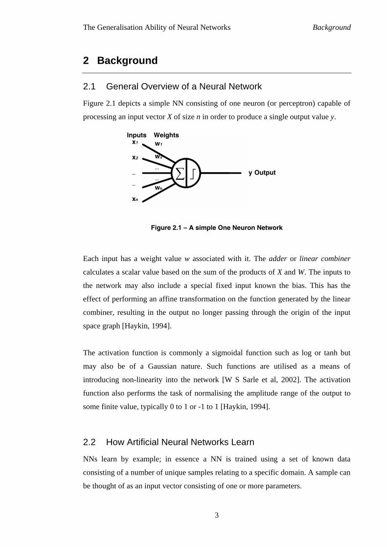
Figure 2.1 depicts a simple NN consisting of one neuron (or perceptron) capable of
processing an input vector X of size n in order to produce a single output value y.
x1
x2
...
...
xn
∑
s
t
Figure 2.1 – A simple One Neu
Each input has a weight value w associated with
calculates a scalar value based on the sum of the p
the network may also include a special fixed inp
effect of performing an affine transformation on th
combiner, resulting in the output no longer passin
space graph [Haykin, 1994].
The activation function is commonly a sigmoidal
may also be of a Gaussian nature. Such funct
introducing non-linearity into the network [W S
function also performs the task of normalising the
some finite value, typically 0 to 1 or -1 to 1 [Hayki
2.2 How Artificial Neural Networks Lea
NNs learn by example; in essence a NN is tra
consisting of a number of unique samples relating t
be thought of as an input vector consisting of one o
3
y Outpu
Inputs Weight
w1p3
w2
…
…
wn
ron Network
it. The adder or linear combiner
roducts of X and W. The inputs to
ut known the bias. This has the
e function generated by the linear
g through the origin of the input
function such as log or tanh but
ions are utilised as a means of
Sarle et al, 2002]. The activation
amplitude range of the output to
n, 1994].
rn
ined using a set of known data
o a specific domain. A sample can
r more parameters.

The Generalisation Ability of Neural Networks Background
Each input vector is presented to the NN and an output vector is generated. The value
of the output vector is then compared to the actual answer, and an error value is
calculated based on the difference between the two answers. This value is then used
to adjust the weights of the NN. There are many different means of deciding when
training should be stopped, these include, stopping once the error falls below a
specific threshold or once a given number of training iterations has been reached (see
section 2.8.3).
Expert systems rely on the developer clearly defining rules or functions that are used
to map input values to their respective output values. NNs on the other hand, employ
a black-box approach to the mapping of inputs to outputs [Sarkar, 1996]. Although
the weights of a network may be viewed, they are generally far too complex to be
translated into values of any real significance to a developer or user.
2.3 Early Developments
McCulloch and Pitt [1943] developed a simple neuron model capable of computing
logic functions. The McCulloch-Pitt neuron was based on the knowledge of
biological neural networks at that time. As a result, the model used a threshold
activation function resulting in all or nothing activity. It also assumed that the state of
a neuron remained static for the life of the network [Young, 2003].
Work done by psychologist Hebb [1949] shed new light on how humans learn. He
discovered that neurons that were fired frequently became stronger and therefore
familiarity reinforced pathways within the brain resulting in learning occurring. The
infrequent use of particular pathways within the brain also resulted in weakening of
the neurons resulting in memory loss.
In the late 1950s Rosenblatt [1958] applied Hebb’s principles of learning to the
McCulloch-Pitt model resulting in adjustable weights being added to the input
connections; this model was known as the perceptron. Initially the connection
weights were set to random values, the network was presented with a problem and an
answer generated in the form of a binary value. If the perceptron generated an answer
4
The Generalisation Ability of Neural Networks Background
that was in error, the weights were adjusted by some constant factor. This resulted in
two basic rules: 1) if the output was one instead of zero the values of the weights
were decreased 2) if the output was zero instead of one the values of the weights
were increased [Young, 2003].
2.4 Single-Layer NNs
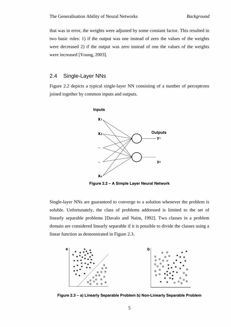
Figure 2.2 depicts a typical single-layer NN consisting of a number of perceptrons
joined together by common inputs and outputs.
F
Single-layer NNs are
soluble. Unfortunately
linearly separable pro
domain are considered
linear function as dem
a
Figure 2.3 – a) Line
Inputs
igure 2.2 – A Simple Layer Neur
guaranteed to converge to a so
, the class of problems addr
blems [Davalo and Naim, 199
linearly separable if it is possi
onstrated in Figure 2.3.
arly Separable Problem b) Non-
5
Outputs
x1
x2
...
...
xn
al
lut
ess
2]
ble
Lin
y1
y2
Network
ion whenever the problem is
ed is limited to the set of
. Two classes in a problem
to divide the classes using a
b
early Separable Problem
The Generalisation Ability of Neural Networks Background
Minksy and Papert [1968] highlighted the problem of linear separability in their
famous paper Perceptrons, which demonstrated that Rosenblatt’s perceptron was
incapable of representing the XOR function.
Minsky and Papert also (incorrectly) conjectured that this problem existed in NNs
with multiple layers which resulted in research in this area coming close to a
complete standstill [Davalo and Naim, 1992].
2.5 The Multi-Layer Perceptron (MLP)
Rumelhart and McClelland [1986] introduced back-propagation (BP) to the world in
their book Parallel Distributed Programming. Dayhoff [1990] states that the concept
of BP was first presented by Werbos [1974], and then independently re-invented by
Parker [1982]1.
BP makes it possible to propagate the error value backwards through the network
that generated it. This algorithm is also not limited to a single layer of adjustable
weights resulting in the development of successful MLPs.
MLPs consist of multiple layers of neurons connected together to perform parallel
computation on an input vector. They are the most popular type of NN architecture
and many concepts which apply to MLPs also apply to other neural network types.
[Swingler, 1996]. Contrary to Minsky and Papert’s claims MLPs are also able to
learn functions capable of classifying non-linearly separable input spaces.
2.6 Finding the Global Minimum in a MLP
BP is a gradient descent algorithm, meaning that it continues to train whilst the error
rate of the network is decreasing. Ideally this method will result in the NNs training
process being stopped when the global minimum has been found. However because
the error surface of the problem space is not known a priori it is possible that the
1 Literature on the history of MLPs varies and contrary to Dayhoff’s statement it may actually be true
that invented the BP algorithm or a similar variation.
6
The Generalisation Ability of Neural Networks Background
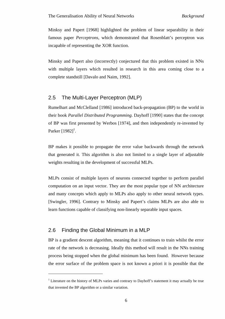
network can stop training at some local minima see Figure 2.4. It is possible that the
local minimum that the network has trained to is a point vastly removed from the
global minimum and will therefore result in poor performance of the network.
Global Minimum
Figure 1.5
Possible start locations
Local Minimum
Figure 2.4 – Starting with different weights can help to overcome the likelihood of
converging on local minima.
Several techniques for reducing the likelihood of convergence to local minima have
been developed, these include shaking and multi-start.
Shaking involves adding noise to the input data in an effort to shake the network
enough to avoid the BP algorithm settling at some local minima.
Multistart exploits the fact that NNs are initialized with random weights therefore
each time a network is initialised it starts in a different area of the input space. The
data is tested on the same network multiple times with different initial starting
weights. Each time the network is trained the connection weights are recorded and
after a sufficient2 number of restarts the network reporting the lowest error value is
deemed to be correct.
However Mitchell [1997] states that the occurrence of convergence to some local
minima may not be of great concern based on the following reasoning:
2 Generally a user specified number of times based on factors such as available time, computational
power, experience and problem space.
7
The Generalisation Ability of Neural Networks Background
“Consider that networks with large numbers of weights correspond to error surfaces
in high dimensional spaces (one dimension per weight). When gradient descent falls
into a local minimum with respect to one of these weights, it will not necessarily be
in a local minimum with respect to other weights. In fact, the more weights in the
network, the more dimensions that might provide escape routes for gradient descent
to fall away from local minimum with respect to this single weight.”
2.7 Generalisation Ability of NNs
2.7.1 Overview of Generalisation
The generalisation ability of NNs could be compared to that of a child learning the
difference between cars and trucks. Provided the child learns from examples that are
accurate about the differing features of cars and trucks they should be able to
correctly classify many vehicles as either one or the other.
Generalisation allows learning to take place using a finite set of examples. If it were
the case that the child needed to be shown one of every model of car and truck made
by man, it is likely that the problem space would grow faster than the child’s ability
to memorize each example. This feature is what distinguishes expert systems from
NNs as the former is generally a tightly constructed, finite set of facts only capable
of classifying problems previously solved by a human expert. NNs on the other hand
have the ability to make decisions using a loosely defined set of self taught rules
learnt using previous examples.
2.7.2 Generalisation Error
Consider again the child in the previous example seeing a truck, this time with a
canopy covering the trailer. Even at first glance the child will make associations with
the vehicle. They will use reasoning to deduce that the object is related to a car or
truck due to similar features and its location within the environment. The child may
then deduce that the vehicle looks like a truck with a lid similar to that of a lunch-box
lid, designed to stop the contents falling out.
8
The Generalisation Ability of Neural Networks Background
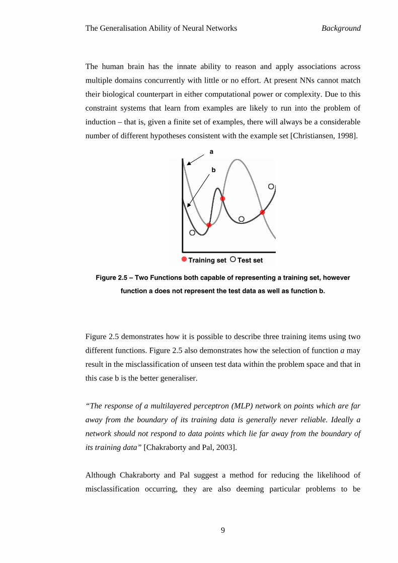
The human brain has the innate ability to reason and apply associations across
multiple domains concurrently with little or no effort. At present NNs cannot match
their biological counterpart in either computational power or complexity. Due to this
constraint systems that learn from examples are likely to run into the problem of
induction – that is, given a finite set of examples, there will always be a considerable
number of different hypotheses consistent with the example set [Christiansen, 1998].
b
t
Figure 2.5 – Two Functions
function a does not
Figure 2.5 demonstrates how i
different functions. Figure 2.5
result in the misclassification o
this case b is the better general
“The response of a multilayer
away from the boundary of it
network should not respond to
its training data” [Chakraborty
Although Chakraborty and P
misclassification occurring, t
Training set Test se
both ca
represe
t is pos
also de
f unsee
iser.
ed perc
s train
data p
and P
al sugg
hey a
a
pable of representing a training set, however
nt the test data as well as function b.
sible to describe three training items using two
monstrates how the selection of function a may
n test data within the problem space and that in
eptron (MLP) network on points which are far
ing data is generally never reliable. Ideally a
oints which lie far away from the boundary of
al, 2003].
est a method for reducing the likelihood of
re also deeming particular problems to be
9
The Generalisation Ability of Neural Networks Background
unclassifiable by the network and as a result human intervention or retraining of the
network would be required.
Schoner [1992] suggests that of the main factors that influence generalisation
performance in NNs two are of particular relevance. The first is the
representativeness of the training set to the problem space. If the training set does not
encapsulate the problem space, the presentation of new data will result in
unpredictable and unreliable output (section 2.10). The second is the size of the NN
i.e. is the network of a sufficient complexity to accurately model the function
representing the problem space (section 2.12).
2.8 Cross Validation Training Methods
The cross validation process attempts to withhold a portion of data from the training
process. Once the training process is complete the data that was withheld is used to
evaluate the performance of the network.
2.8.1 Holdout Cross Validation
The simplest method of training known as holdout cross-validation involves splitting
the available data into two sets; one for training, the other for testing [Schneider,
1997]. Once the NN has learnt the training set, the weights in the network are fixed
and the testing set is used to verify how well the network classifies on unseen data.
2.8.2 k-fold Cross Validation
k-fold cross validation is a variation on the holdout method that involves splitting the
data set into k approximately equal segments. One set is then left out for testing
whilst the other k-1 sets are used for training. This process is repeated k times with a
different k set held out for testing.
k-fold cross validation allows each sample in the data to be used for both training and
testing which can be advantageous when only small sets of data are available.
Another advantage of k-fold training is that k may be varied to suit the specific
10
The Generalisation Ability of Neural Networks Background
purpose of the network or data. The logical extreme of k-fold cross validation results
in k = n where n is the number of available samples in the data set. This is generally
known as leave-one-out cross validation.
2.8.3 Stopped Training
Stopped training is a method that was implemented in an effort to avoid overfitting
(section 2.11.1). The principle of stopped training is to employ the holdout cross
validation technique frequently to the network during training. Each time the testing
set is applied to the network an error value is recorded. Once the error value begins
to rise it is suggested that training stop as this is the point when generalisation has
reached its estimated maximum [Schoner, 1992].
Given the fact that the testing set has been used repeatedly during the training
lifecycle it is recommended that the initial set of data be broken into three sets;
training, testing and validation. The validation set is used to measure the
performance of the network once it has stopped.
2.9 Prior Knowledge
Prior knowledge (also known as hints) is a means by which additional information
not present in the sample data may be incorporated into the learning process. Hints
can be used as a means of constraining the induction process of the NN [Abu-
Mostafa, 1990; S C Suddarth Y L Kergosien, 1991].
F. M. Richardson et al [Date Unknown] produced work relating to the
implementation of prior knowledge as weights in the network. An incremental
approach was taken, whereby a NN was initially trained on two of four existing
patterns. Once training was complete the network weights were used as the initial
weights for the retraining of the two previous patterns incorporated with a third
‘new’ pattern. This process was then repeated with a fourth pattern added. The
results produced by this training method were found to be of significantly better
quality than those of a standard NN trained using all four patterns at once.
11
The Generalisation Ability of Neural Networks Background
2.10 Data Sets for Selection and Training
2.10.1 Selecting Appropriate Data
The human perception of patterns in a complex problem space can differ greatly to
that of the NN employed to classify the data. Therefore the selection of inappropriate
data is likely to result in poor generalisation. A good training set has the minimum
number of patterns representing all the possible problem characteristics; such a
training set supplies the network with all the necessary information to correctly
generalize over unknown patterns [Tamburini and Davoli, 1994]. However more
recently software such as the Weka suite of machine learning algorithms [Witten and
Frank, 2000] allow for a more accurate analysis of the patterns found in data sets.
Tamburini and Davoli [1994] state that when two samples x and y are similar
generalisation may benefit from the omittance of either x or y. Similar patterns
should have little effect on the function being learnt by the NN. Avoiding data
redundancy reduces the risk of x being in the training set and y in the test set. Such an
occurrence results in an trivial classification which is not really testing the
generalisation of the network [Abu-Mostafa, 1990].
Reducing the overall number of instances through the omittance of similar instances
may help to reduce the size of the data set being trained and in turn reduce training
times. However omitting instances that occur frequently within a domain may
actually reduce the overall performance of the NN due to fact that the network may
not be biased enough towards instances which naturally occur more frequently.
It is important to select samples across all classes within a given input space. The
more equally distributed the classes the more symmetric the error surface will be
[Duch and Kordos, 2004]. It is also important that classes within the data set do not
overlap as this will produce misclassification. If overlapping occurs the data will
suffer effects similar to that of overfitting [Chakraborty and Pal, 2003]. Overlapping
in this sense may be unavoidable due to the sheer nature of the data; however it may
be possible to reduce this effect by adjusting the architecture of the network.
12
The Generalisation Ability of Neural Networks Background
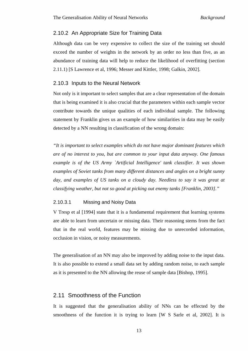
2.10.2 An Appropriate Size for Training Data
Although data can be very expensive to collect the size of the training set should
exceed the number of weights in the network by an order no less than five, as an
abundance of training data will help to reduce the likelihood of overfitting (section
2.11.1) [S Lawrence et al, 1996; Messer and Kittler, 1998; Galkin, 2002].
2.10.3 Inputs to the Neural Network
Not only is it important to select samples that are a clear representation of the domain
that is being examined it is also crucial that the parameters within each sample vector
contribute towards the unique qualities of each individual sample. The following
statement by Franklin gives us an example of how similarities in data may be easily
detected by a NN resulting in classification of the wrong domain:
“It is important to select examples which do not have major dominant features which
are of no interest to you, but are common to your input data anyway. One famous
example is of the US Army `Artificial Intelligence' tank classifier. It was shown
examples of Soviet tanks from many different distances and angles on a bright sunny
day, and examples of US tanks on a cloudy day. Needless to say it was great at
classifying weather, but not so good at picking out enemy tanks [Franklin, 2003].”
2.10.3.1 Missing and Noisy Data
V Tresp et al [1994] state that it is a fundamental requirement that learning systems
are able to learn from uncertain or missing data. Their reasoning stems from the fact
that in the real world, features may be missing due to unrecorded information,
occlusion in vision, or noisy measurements.
The generalisation of an NN may also be improved by adding noise to the input data.
It is also possible to extend a small data set by adding random noise, to each sample
as it is presented to the NN allowing the reuse of sample data [Bishop, 1995].
2.11 Smoothness of the Function
It is suggested that the generalisation ability of NNs can be effected by the
smoothness of the function it is trying to learn [W S Sarle et al, 2002]. It is
13
The Generalisation Ability of Neural Networks Background
considered important that when a small change is made to an input on the network it
reflects a small change in output. This is emphasised by Chakraborty and Pal [2003]
in their statement regarding the reliability of inputs located too far away from the
input space (see section 2.7.2).
Additionally in the case of limited training sets and limited topological complexities,
good generalisation performance can be obtained if the neural model of the problem
implies a smoothing operation in the available data. Smoothness constraints can be
introduced, in the case of MLPs, by constraining network complexity [Burrascano,
1992]
2.11.1 Underfitting and Overfitting
One of the most important issues that arise when training a NN is that of avoiding
underfitting and overfitting. If a NN’s architecture is insufficiently complex the
model will lack flexibility resulting in a high bias within the input space known also
as underfitting. Conversely if the architecture of the model is too complex the NN
will fit the data so tightly that any noise evident in the data will also be trained into
the network resulting in overfitting [Geman S et al, 1992]. This phenomenon results
in poor generalisation of new data due to the fact that the network has learned the
training data rather than the problem space.
2.12 Network Architecture
2.12.1 Neural Network Complexity
An MLP with two hidden layers can be used as universal function approximators
[Hornik, 1991; Hornik, 1993; Leshno, Lin et al., 1993; Bishop, 1995]. Therefore
applying the principle known as Occam’s Razor3 which states: of two solutions
known to sufficiently solve a problem the simpler of the two should be used, will
help to minimise the complexity of MLPs [Duch and Grabczewski, 1999; Aran and
3 Of two solutions known to sufficiently solve a problem the simpler of the two should be chosen.
14
The Generalisation Ability of Neural Networks Background
Alpaydin, 2003]. The optimum number of hidden units, however, can often only be
found by trial and error [Schoner, 1992].
Reducing the size of the network not only helps improve generalisation it also
increases the computational speed of the system. There is roughly a linear
relationship between the network size and computational speed.[Messer and Kittler,
1998]
2.12.2 Feed-Forward and Feedback Neural Networks
Feed-Forward (FF) and Feedback (FB) networks, also known as Recurrent
Networks, are the two most common types of NNs. A FF networks can be thought of
as a directed acyclic graph, where neurons within a MLP only transfer data to their
successors. FB networks on the other hand have connections to neighbour and
predecessor neurons within the network as well as successors. Therefore FB
networks can also be thought of as directed cyclic graphs. FB NNs are generally
more difficult to train than FF networks [Sarle, 1995].
2.12.3 Weight Initialization
In general, initializing the network with small weights allows them to be updated
smoothly thereby avoiding local minima. It is suggested to initialize and to train the
network many times with different sets of small initial weights [Schmidt, Raudys et
al., 1993] .
2.13 Improving Generalisation
Many factors within a NN affect generalisation of importance are network size, prior
knowledge, stopping at an optimal time during training, properties of the training set
and the initial weights [Sarkar, 1996; Atiya and Ji, 1997]. The method of training has
no effect on the error surface of the function generated by the NN [Duch and
Adamczak, 1998]. However, the selected training method is likely to affect the time
and computational power required to train a network and is therefore still a necessary
design consideration.
15
The Generalisation Ability of Neural Networks Methodology
3 Methodology
3.1 Data Set Selection and Preparation
3.1.1 Choosing Appropriate Data Sets
In order to test the effect of the size of a data set on the generalisation ability of a NN
it would be necessary to select a data set that was large enough to be separated into
subsets. The reasoning behind this decision was that comparing the test results of two
completely different data sets is likely to introduce the added complexity of
determining whether the data sets themselves are in fact suitably comparable.
Breaking the data set down into subsets at least ensures that there is maximum
compatibility within the data set itself.
3.1.2 Selection of Random Subsets.
The subsets were produced using a simple C++ program which generated a list of
unique random numbers between a specific range of values. The list was then used to
select the appropriate instances from an initial master file and place them into a new
file in the order of the random list. This process was also used to shuffle data sets
when 100% of the data was used, ensuring that the data sets were not ordered
arbitrarily due to the recording process used to collect the samples.
3.1.3 Unique Identifiers
Each instance within a given data set was assigned a unique ID number. Although
this was not initially deemed necessary it proved a useful means of visually
inspecting data sets to verify that two data sets were indeed significantly different
after random selection.
The assignment of the identifier became increasingly beneficial as it proved to be an
effective way of tracking particular instances within the data sets (see section 3.8 for
further details).
16
The Generalisation Ability of Neural Networks Methodology
3.1.4 Mushroom Data Set
The mushroom data set was sourced from the University of California Irvine’s (UCI)
Machine Learning Repository. It contains 22 discrete attributes and 2 classes (edible
and poisonous). The distribution for edible and poisonous classes is 4208 (51.8%)
and 3916 (48.2%) respectively for a total of 8214 instances. The only data missing
from the mushroom set is from the 11th attribute and of this a total of 11% of the
attribute values are missing.
The number of instances was ultimately the deciding factor in choosing this data set,
as even at a tenth of its original size it is comparable to many of the smaller data sets
available in the UCI’s repository.
The attribute values are represented alphabetically in the original data set and it has
therefore been necessary to convert them to numeric values. In order to do this the
following calculation is made where v = [a0 , a1 , …. , aN] represents a vector of the
values for a given attribute:
Nj
ja =
The net effect of this conversion is that the values assigned to v are normalised and
equally distributed with respect to the other values within each attribute. It is
important to note that this method has the effect of ordering the values within each
attribute and may result in loss of performance. However due to the networks ability
to classify to a considerably low error rate using this technique it is deemed that for
the purpose of this research this method is sufficient.
3.1.5 Functional Data Sets
It is not usually possible to determine the complexity of a function learned by a NN.
In order to perform these tests it was necessary to create a selection of artificial data
sets, capable of generating meaningful test results whilst still being comprehensible
enough to be comparable to each other. Graphis v2.34 was used to generate four 4 Graphis is produced by Kylebank Software www.kylebank.com.
17
The Generalisation Ability of Neural Networks Methodology
three-dimensional graphs of differing complexity. The values of each graph were
then normalised (to the range zero to one) and outputted to individual files. The x and
y co-ordinates of the graph are used as input values to a NN and the z co-ordinate is
treated as the desired output value from the NN. The resolution of each grid was 35 x
35 as this was determined to be a sufficient number to create enough instances per
data set for measurable results in a constrained amount of time.
3.2 Neural Network Program
The NN program used for training and testing was provided by Xu (2004). The
program consisted of a basic feed-forward back-propagation NN. The adjustment of
weights within the network was performed at the end of each iteration or epoch. As a
result the number of adjustments made to the each weight is equal to the number of
training epochs.
It would also have been feasible to make the weight adjustments after the
classification of each instance. Therefore increasing the number of weight
adjustments to be equal to the number of epochs multiplied by the number of
instances. Due to the vast amount of training required to provide sufficient results for
the key areas within this research it was decided that this would not be a necessary
adjustment. This would be revised if it was found that the NN was unable to train
sufficiently on any of the data it was presented with.
The program performed several output operations for reporting purposes; this
included the recording of the error rate during training after every ten epochs.
Another feature implemented after receiving the program was the generation of a log
file. This was implemented as a means of recording information such as the lowest
training error reached by the network, the epoch at which this was reached and other
general information such as the number of nodes in the input, hidden and output
layers of the particular NN that created the file.
18
The Generalisation Ability of Neural Networks Methodology
3.3 Training Process
10-fold cross validation was performed on each data set (or subset). Training of the
NN was halted when one of two conditions was met; 1) the error level had reached a
threshold of 10-7, 2) the number of training epochs had exceeded some given
threshold. This threshold was initially chosen because the original code for the NN
implemented this stopping condition. However it was often the case that an error this
low could not be reached, therefore it was often necessary to stop the network after a
specific number of epochs.
The reason for training down to such a low error rate stemmed from the need to
know exactly how well they had been classified. It would be entirely acceptable to
threshold the binary output produced when classifying the mushroom data set. For
example, an error rate lower than 0.2 is considered to be zero and an error rate higher
than 0.8 is considered to be one. However had the training and testing been
implemented using this method, the difference in the generalisation error between
individual tests that clearly exceeded the nominated thresholds would not be
measurable. Therefore the option that has been chosen is to compare the actual error
rates produced during testing as this is a better indication of the generalisation
performance.
On completion of training, the weights of the NN were saved to a file and an entry
appended to a log file which includes information relevant to the training process
such as the final error, lowest error and the epoch at which the lowest error was
reached.
During the training process the NN was re-started if it appeared to be converging to
some local minima. Re-starting was an automated process that allowed the NN to be
self-regulating and involved the re-generation of the initial weights in the network
with a new random seed. Re-generation was triggered when the following two
conditions were met simultaneously; 1) the error rate had not fallen below 3-3 and 2)
the difference between the previous epoch’s error and the current epochs error was
less than 5-6. These figures were settled upon after lengthy analysis of the error rate
during the networks training process. It was often the case that if the rate at which the
19
The Generalisation Ability of Neural Networks Methodology
error was dropping by fell below 5x10⁻⁶ before it reached an error rate of less than
3x10⁻³ the network would stall (perhaps due to it being caught in some local minima).
However when the network was restarted with a different set of initial weights, local
minima could often be avoided and the network would train to a much lower error
rate.
Due to the self-regulating nature of the training process it was possible that the last
error reached by the NN was not the lowest error reached during training. If this was
the case the information stored in the log file was used to re-train the network down
to the lowest error. Although this process resulted in a greater cost-of-training
overhead it ensured that the NN was not stopped prematurely. Often it was the case
that the lowest error (stopping condition 1) was reached after several restarts,
therefore stopping the NN at the first lowest error encountered without any further
re-generation of weights may result in a set of sub-optimal weights being generated.
In turn the testing phase would yield inconsistent results and ultimately result in any
conclusions made being inaccurate and misleading.
The number of epochs permitted before training was halted, varied between 30,000
and 100,000 depending on the size of the data. The NN appeared to converge in
fewer epochs on larger sets of data and the limits imposed on the training process
were deemed to be an adequate number of training iterations for the NN to converge
to an error level sufficiently close to the optimal error level. Determining the
appropriate limits involved initial training runs of up to 600,000 epochs. After these
runs had completed, the error levels were examined and limits were generated based
on the point at which continuing training failed to produce significant improvements
in the error levels. The analysis of error levels throughout training was possible due
because the program was tailored to output (to file) the current error level at every
tenth epoch.
3.4 Neural Network Architecture
The NN consisted of an input layer, one hidden layer and an output layer. Numerous
trials were conducted in order to determine the appropriate number of hidden nodes
within the NN. These trials included varying the initial weights and the number of
20
The Generalisation Ability of Neural Networks Methodology
hidden nodes within the network. The nodes themselves were implemented using a
sigmoid activation function.
Were training and testing of the mushroom data set was performed; eight hidden
nodes were determined to give the best performance across a range of training set
sizes5. The functional data sets performed well using only two hidden nodes, as these
data sets are comparatively smaller and less complex than the mushroom data set.
3.5 Training Data Size
In order to test how the size of training data effects generalisation it was obviously
going to be necessary to train the NN on data sets of different sizes. Although the
UCI provides access to many data sets of varying sizes suitable for performing such
tests it is possible that other differences such as the number of attributes and the
accuracy of the data may invalidate any size comparisons made between two data
sets.
For example the UCI’s Diabetes data set consists of 768 instances, approximately a
tenth of the size of the mushroom data set. If both data sets are used to train a NN it
is possible that the results may be different (i.e. one out-performs the other).
Although conclusions may be drawn regarding the reasons behind this, it is not safe
to assume that either data set’s performance is related to its size. This is because
although it is possible to reduce the mushroom data set down to a subset of 768
instances it is not possible to increase the diabetes data set in order to match the size
of the mushroom data set. There are also a number of reasons other than size that
might affect performance such as the number of attributes, accuracy of data and
whether the attributes are discrete or continuous.
Due to the fact that these problems were likely to arise it was decided that a data set
should be selected that was large enough to allow it to be reduced into subsets that
were relative to the size of other data sets within the UCI’s repository. Random
subsets were produced using 10%, 25%, 50% & 75% of the mushroom data set as
this was deemed to be an appropriate size for subset selection. Four selections of
5 See Section 3.5 for details regarding the actual training set sizes used.
21
The Generalisation Ability of Neural Networks Methodology
each size were created resulting in a total of sixteen subsets being generated. The
purpose of generating multiple subsets was to enable the result of testing to be
averaged in order to refine the accuracy of the test results produced. The choice of
only four subsets per test was made due to time constraints and it is likely that using
a larger number of subsets would produce more accurate results (see section 6.2 for
further details).
3.6 Inputs to the Network
The focus of this section is to examine the effects a NN’s inputs have on the
performance of generalisation. Once again the mushroom data set was used to
perform the training of the NN as it possesses a significantly large number of
attributes.
Initially it was decided that the process of testing the effect of the inputs on the NN
would involve re-creating the mushroom data set with different numbers of
attributes. The newly created data sets would then be used to train the NN and the
result of each test would be compared.
Section 3.4 describes the process involved in determining the appropriate size of the
NN. This process would therefore suggest that reducing the number of attributes
within the mushroom data set is likely to result in the architecture of the network
requiring modifications too. After some initial testing it was confirmed that this was
correct and that eight hidden nodes was not an appropriate number when the training
set had a reduced set of attributes, this led to the question; Are NNs of different
architectures comparable in their generalisation ability of a domain? In order to
answer this question it would be necessary to perform numerous tests involving the
size of the hidden layer in the NN and its affect on generalisation. Therefore it was
decided that this approach, although interesting, would not become part of the testing
within this thesis as it related to the architecture of the NN as much as it related to
the inputs themselves.
An alternative solution was devised in order to solve the architectural dilemma.
Rather than testing the effects the number of inputs has on the NN, the attributes
influence on the generalisation ability was to be tested instead. As a result the NN
22
The Generalisation Ability of Neural Networks Methodology
program was re-configured so that it was possible to ignore particular6 attribute’s
values and instead replace them with the value one.
To test the validity of this process a leave-one-out approach was taken using 10% of
the mushroom data set. This approach involved training the network 22 times on 21
active attributes, each time leaving a different attribute inactive. Due to time
constraints it was not possible to perform 10-fold cross-validation for each possible
combination of test as this would have required 220 training and testing session. For
the purposes of this experiment it was therefore necessary to produce a random
subset of 780 instances, the first 702 for training and the remaining 78 for testing7.
This proved to be successful8 based on the fact that the NN was able to train down to
an error rate of 10-7, suggesting that the NN was not being adversely affected by the
in-active parameters. Testing of the final weights generated by this process produced
an average error rate in the order of 10-4. This figure is comparative to those recorded
in previous testing session9, thereby indicating that this method showed significant
potential.
As mentioned previously time constraints governed the amount of training and
testing that could be achieved. Using every combination of active and in-active
attributes would result in training being performed in the order of 222 times. Now that
a method for testing the influence of the attributes on NN had been formalised a
heuristic was therefore needed to determine which combinations of attributes would
be tested.
On closer inspection of the error rates produced by the test data it was clear due to
the similarities of each result that no insight would be gained into the affects the in-
active parameters had on the NNs performance during this process. Another
approach would therefore have to be taken and as a result attention was turned to the
6 These are specified by the user at the beginning of training and testing. 7 The implications of this are discussed in section 6.2. 8 The results produced are comparative to those produced when all 22 parameters are active. 9 Section 4.3 outlines the results of testing all 22 attributes on 10% of the mushroom data set.
23
The Generalisation Ability of Neural Networks Methodology
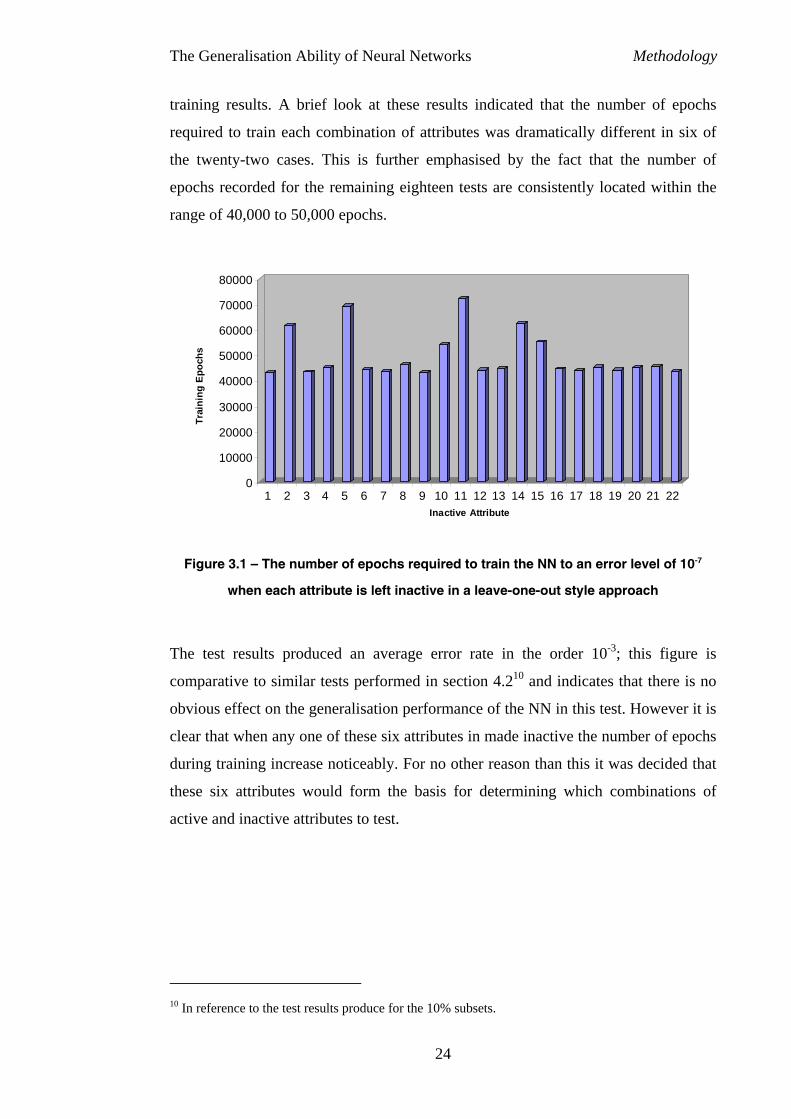
training results. A brief look at these results indicated that the number of epochs
required to train each combination of attributes was dramatically different in six of
the twenty-two cases. This is further emphasised by the fact that the number of
epochs recorded for the remaining eighteen tests are consistently located within the
range of 40,000 to 50,000 epochs.
0
10000
20000
30000
40000
50000
60000
70000
80000
Trai
ning
Epo
chs
1 2 3 4 5 6 7 8 9 10 11 12 13 14 15 16 17 18 19 20 21 22Inactive Attribute
Figure 3.1 – The number of epochs required to train the NN to an error level of 10-7
when each attribute is left inactive in a leave-one-out style approach
The test results produced an average error rate in the order 10-3; this figure is
comparative to similar tests performed in section 4.210 and indicates that there is no
obvious effect on the generalisation performance of the NN in this test. However it is
clear that when any one of these six attributes in made inactive the number of epochs
during training increase noticeably. For no other reason than this it was decided that
these six attributes would form the basis for determining which combinations of
active and inactive attributes to test.
10 In reference to the test results produce for the 10% subsets.
24
The Generalisation Ability of Neural Networks Methodology
r
01 02 03 04 05 06 07 08
6 0 1 0 0 1 0 0 0
10 0 1 0 0 1 0 1 0
14 0 1 1 0 1 0 1 1
18 1 1 1 0 1 1 1 1
22 1 1 1 1 1 1 1 1Att
rib
ute
Nu
mb
er
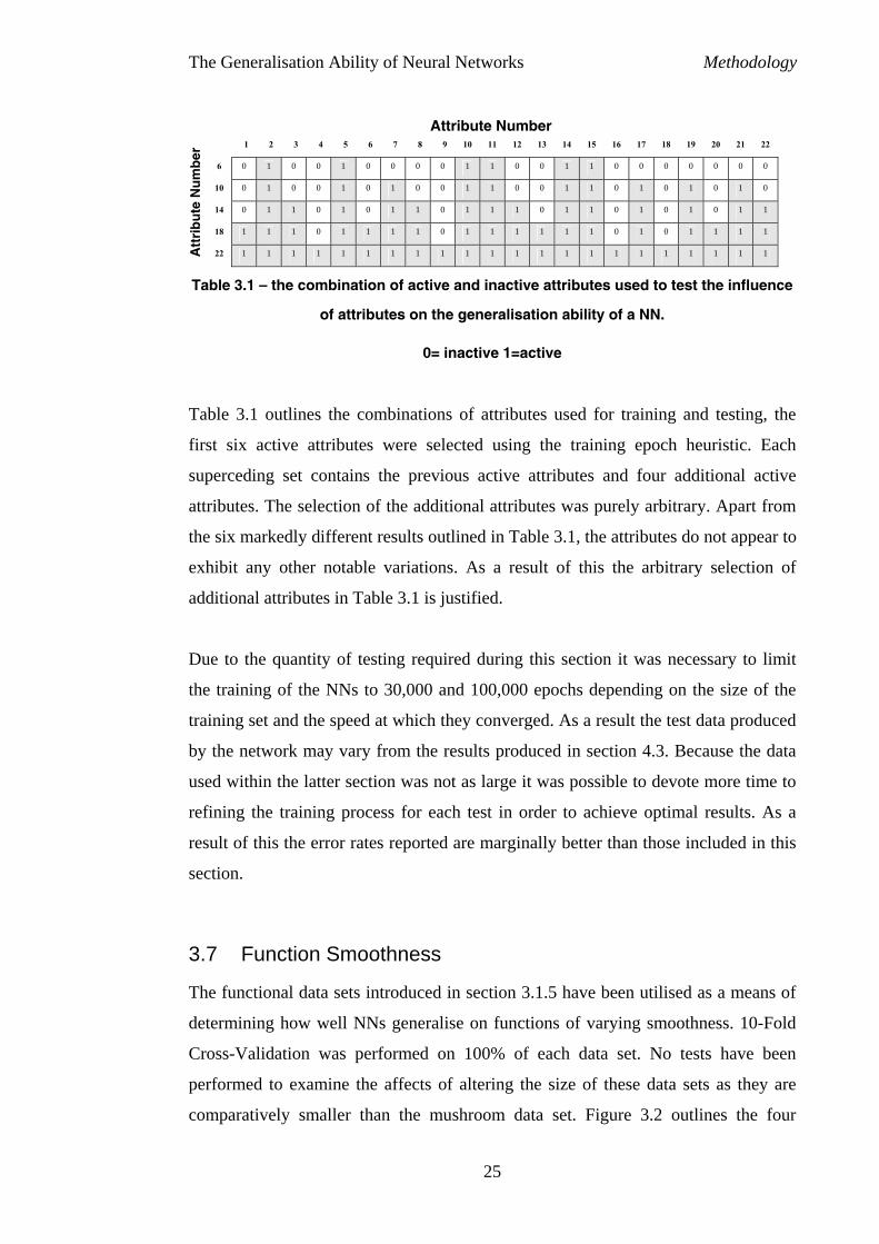
Table 3.1 – the combination of ac
of attributes on
Table 3.1 outlines the combinat
first six active attributes were
superceding set contains the pr
attributes. The selection of the a
the six markedly different results
exhibit any other notable variat
additional attributes in Table 3.1
Due to the quantity of testing re
the training of the NNs to 30,00
training set and the speed at whic
by the network may vary from t
used within the latter section wa
refining the training process for
result of this the error rates repo
section.
3.7 Function Smoothne
The functional data sets introduc
determining how well NNs gene
Cross-Validation was performe
performed to examine the affect
comparatively smaller than the
Attribute Numbe
09 10 11 12 13 14 15 16 17 18 19 20 21 220 1 1 0 0 1 1 0 0 0 0 0 0 0
0 1 1 0 0 1 1 0 1 0 1 0 1 0
0 1 1 1 0 1 1 0 1 0 1 0 1 1
0 1 1 1 1 1 1 0 1 0 1 1 1 1
1 1 1 1 1 1 1 1 1 1 1 1 1 1
tive and inactive attributes used to test the influence
the generalisation ability of a NN.
0= inactive 1=active
ions of attributes used for training and testing, the
selected using the training epoch heuristic. Each
evious active attributes and four additional active
dditional attributes was purely arbitrary. Apart from
outlined in Table 3.1, the attributes do not appear to
ions. As a result of this the arbitrary selection of
is justified.
quired during this section it was necessary to limit
0 and 100,000 epochs depending on the size of the
h they converged. As a result the test data produced
he results produced in section 4.3. Because the data
s not as large it was possible to devote more time to
each test in order to achieve optimal results. As a
rted are marginally better than those included in this
ss
ed in section 3.1.5 have been utilised as a means of
ralise on functions of varying smoothness. 10-Fold
d on 100% of each data set. No tests have been
s of altering the size of these data sets as they are
mushroom data set. Figure 3.2 outlines the four
25
The Generalisation Ability of Neural Networks Methodology
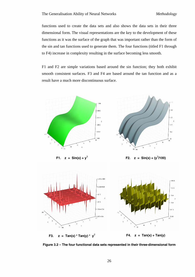
functions used to create the data sets and also shows the data sets in their three
dimensional form. The visual representations are the key to the development of these
functions as it was the surface of the graph that was important rather than the form of
the sin and tan functions used to generate them. The four functions (titled F1 through
to F4) increase in complexity resulting in the surface becoming less smooth.
F1 and F2 are simple variations based around the sin function; they both exhibit
smooth consistent surfaces. F3 and F4 are based around the tan function and as a
result have a much more discontinuous surface.
F1. z = Sin(x) + y3 F2. z = Sin(x) + (y3/100)
F3. z = Tan(x) * Tan(y) * y2 F4. z = Tan(x) + Tan(y)
Figure 3.2 – The four functional data sets represented in their three-dimensional form
26
The Generalisation Ability of Neural Networks Methodology
Each data set consisted of 1225 instances which were calculated using 35 x 35 unit
matrix of values ranging between -10 and 10. These values represented the values of
the x and y coordinates of the four data set functions, and were evenly distributed
across the specified range.
3.8 Prior Knowledge and the Selection of Training Data
The research contained within this section involves the combination of two of the
five original concepts chosen for improving generalisation; prior knowledge and
training set selection. This combining of concepts resulted followed a discussion
with Cameron-Jones [2004] regarding the use of prior knowledge for the purpose of
stacked generalisation [Wolpert, 1992], a hybrid approach to machine learning that
“is a general method of using a high-level model to combine lower-lever models to
achieve greater predictive accuracy” [Ting and Witten, 1997].
The stacked generalisation approach although valid, had already been successfully
implemented; it did however bring to the foreground the idea of re-using test results
produced by a classifier. As a result a method was produced that involved using the
test results produced by the NN to determine whether it was possible to identify
instances capable of improving the generalisation of the NN. The intention during
this process was not to build an entire training set, but instead to seed the training set
with selective instances capable of improving the overall performance of the
network.
The process of building a more robust training set was one of a top down approach
and began by assessing the results generated by the 10% subsets used in section 4.3
(testing the affects of the size of the training data on generalisation) (see Table 3.2).
27
The Generalisation Ability of Neural Networks Methodology
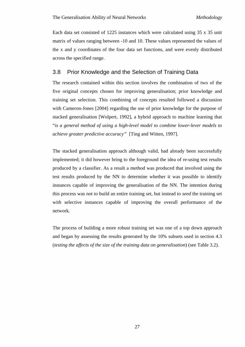
Test Data 1 Test Data 2 Test Data 3 Test Data 4 0.000002 0.000709 0.011404 0.000003 0.000023 0.000422 0.000147 0.000248 0.012147 0.042776 0.000863 0.000001 0.000074 0.000003 0.014354 0.000003 0.014160 0.009628 0.000001 0.000010 0.000003 0.020063 0.011466 0.014040 0.005499 0.000020 0.012837 0.035177 0.000001 0.013653 0.001405 0.000002 0.001538 0.000003 0.000002 0.028574 0.000006 0.008785 0.000004 0.000152
Table 3.2 – Results generation in section 4.3 using 10% of the mushroom data set
With no real certainty as to what was required to build a better training set it was
decided that only test sets that performed at a higher error rate than 10-4 would be
examined further. The shaded cells within Table 3.2 represent the selected test sets
and represent almost 50% of the results produced. This is similar to Quinlan’s
[1983] windowing approach whereby the selection of training instances for each
subsequent test is taken from the poorest results of the previous tests.
The poor performance exhibited by these particular data sets is likely to be associated
with the fact that the test sets contain values that are not sufficiently represented by
their respective training sets. The output files of the selected test sets (produced by
the NN) (section 3.2) during training were then examined in order to determine
which instances performed most poorly. In order to make this decision the difference
between the target and actual output was calculated for each instance within a test
set. If the difference was greater than 0.005 the ID number for the instance would be
outputted to a results file for later use. The choice for the difference threshold was
one of trial and error, with the final threshold producing 75 instances in total. This
level seemed appropriate as it was almost one entire fold of a data set derived from
10% of the mushroom data set. The distribution of the selected instances was
considerably even at 42% edible and 58% poisonous.
Two new data sets were then compiled; one consisting of the 75 selected instances
and the other consisting of the remaining 7715 mushroom instances. Four new
training sets of 10% were then randomly selected from the latter data set. Once
28

The Generalisation Ability of Neural Networks Methodology
created the first 75 instances in each set were replaced with the 75 selected instances.
Leaving them at the head of the data set rather than randomly distributing them
throughout the set meant they would be contained within the first fold of the cross
validation process making their affect on the NN easier to detect. With this
completed, training and testing were carried out as normal.
29
The Generalisation Ability of Neural Networks Results and Discussion
4 Results and Discussion
4.1 Function Smoothness
0.000
0.001
0.002
0.003
0.004
0.005
0.006
0.007
0.008
Ave
rage
Err
or R
ate
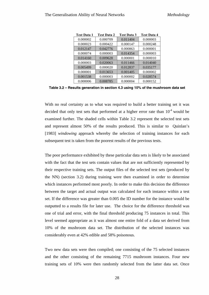
4
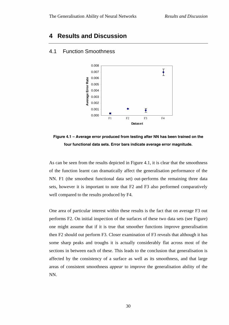
Figure 4.1 – Average error p
four functional data se
As can be seen from the resu
of the function learnt can dr
NN. F1 (the smoothest func
sets, however it is important
well compared to the results p
One area of particular interes
performs F2. On initial inspe
one might assume that if it
then F2 should out perform F
some sharp peaks and troug
sections in between each of t
affected by the consistency
areas of consistent smoothne
NN.
F1 F2 F3 F
Dataset
roduced from testing after NN has been trained on the
ts. Error bars indicate average error magnitude.
lts depicted in Figure 4.1, it is clear that the smoothness
amatically affect the generalisation performance of the
tional data set) out-performs the remaining three data
to note that F2 and F3 also performed comparatively
roduced by F4.
t within these results is the fact that on average F3 out
ction of the surfaces of these two data sets (see Figure)
is true that smoother functions improve generalisation
3. Closer examination of F3 reveals that although it has
hs it is actually considerably flat across most of the
hese. This leads to the conclusion that generalisation is
of a surface as well as its smoothness, and that large
ss appear to improve the generalisation ability of the
30
The Generalisation Ability of Neural Networks Results and Discussion
The error bars in Figure 4.1 suggest an alternative and somewhat contradictory
conclusion to the previous statement. It would seem that although the data set
appears to perform well it may the NN may be suffering from underfitting in such a
way that the overall average performance is quite misleading and may result in
serious interpretation.
Train Test
0.000694 0.0020630.000919 0.0000320.000923 0.0000010.000694 0.0020610.000922 0.0000070.000693 0.0020710.000694 0.0020600.000922 0.0000040.000919 0.0000310.000922 0.000006
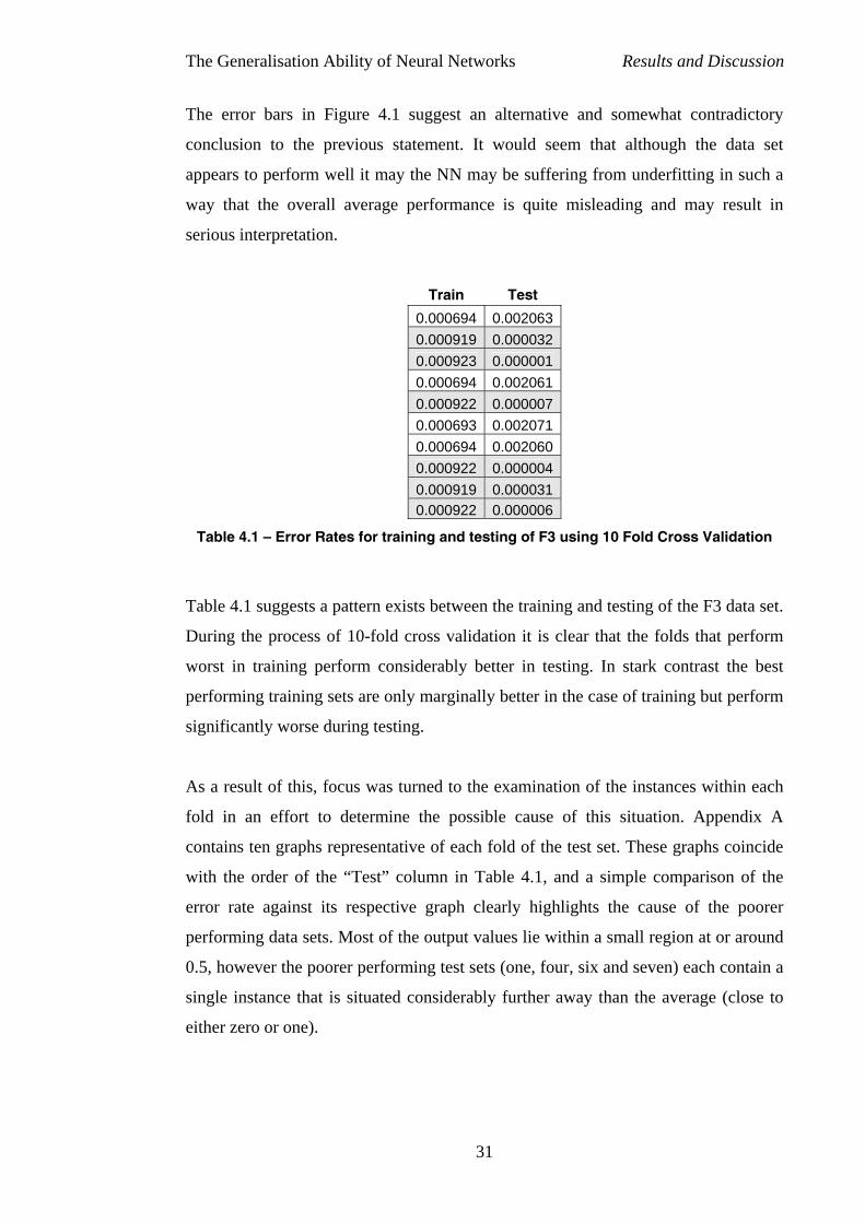
Table 4.1 – Error Rates for training and testing of F3 using 10 Fold Cross Validation
Table 4.1 suggests a pattern exists between the training and testing of the F3 data set.
During the process of 10-fold cross validation it is clear that the folds that perform
worst in training perform considerably better in testing. In stark contrast the best
performing training sets are only marginally better in the case of training but perform
significantly worse during testing.
As a result of this, focus was turned to the examination of the instances within each
fold in an effort to determine the possible cause of this situation. Appendix A
contains ten graphs representative of each fold of the test set. These graphs coincide
with the order of the “Test” column in Table 4.1, and a simple comparison of the
error rate against its respective graph clearly highlights the cause of the poorer
performing data sets. Most of the output values lie within a small region at or around
0.5, however the poorer performing test sets (one, four, six and seven) each contain a
single instance that is situated considerably further away than the average (close to
either zero or one).
31
The Generalisation Ability of Neural Networks Results and Discussion
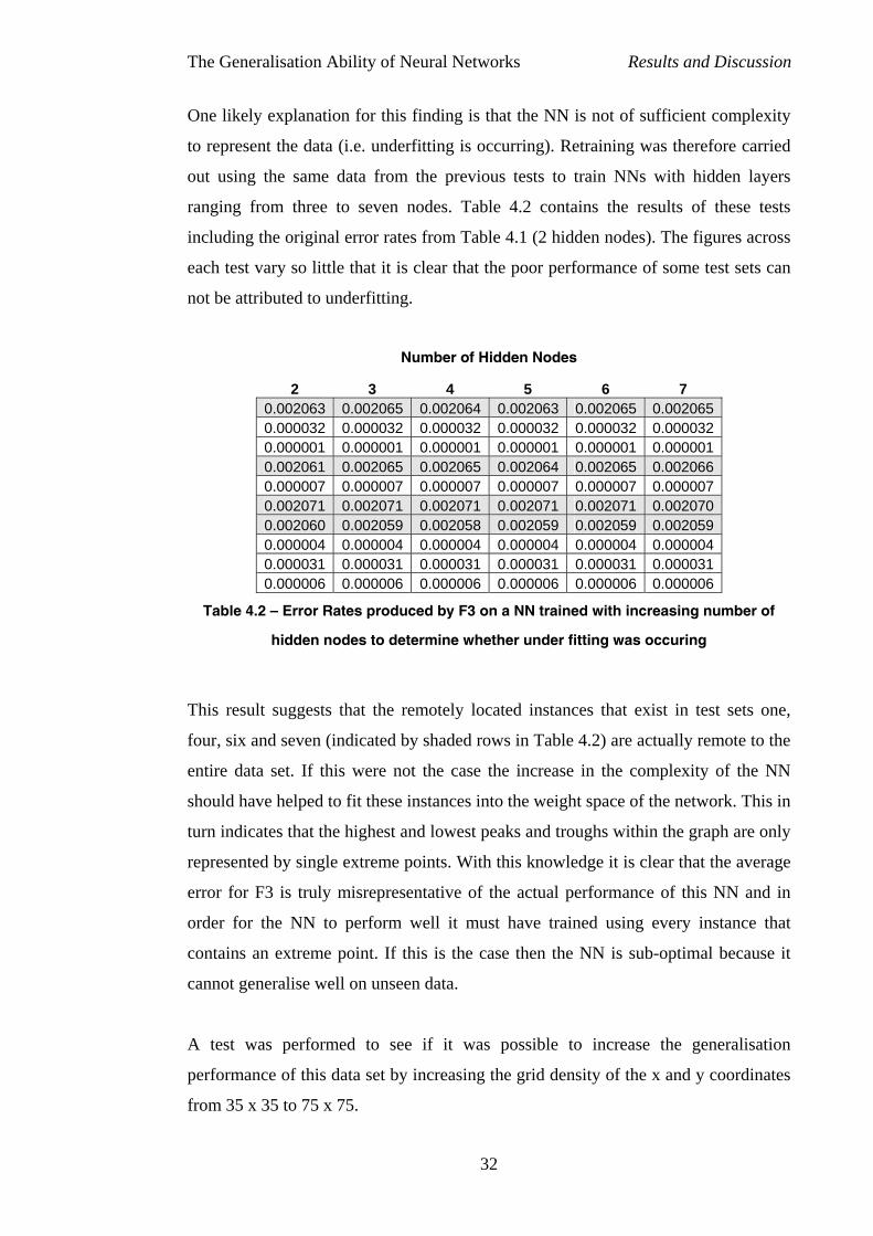
One likely explanation for this finding is that the NN is not of sufficient complexity
to represent the data (i.e. underfitting is occurring). Retraining was therefore carried
out using the same data from the previous tests to train NNs with hidden layers
ranging from three to seven nodes. Table 4.2 contains the results of these tests
including the original error rates from Table 4.1 (2 hidden nodes). The figures across
each test vary so little that it is clear that the poor performance of some test sets can
not be attributed to underfitting.
Number of Hidden Nodes
2 3 4 5 6 7 0.002063 0.002065 0.002064 0.002063 0.002065 0.002065 0.000032 0.000032 0.000032 0.000032 0.000032 0.000032 0.000001 0.000001 0.000001 0.000001 0.000001 0.000001 0.002061 0.002065 0.002065 0.002064 0.002065 0.002066 0.000007 0.000007 0.000007 0.000007 0.000007 0.000007 0.002071 0.002071 0.002071 0.002071 0.002071 0.002070 0.002060 0.002059 0.002058 0.002059 0.002059 0.002059 0.000004 0.000004 0.000004 0.000004 0.000004 0.000004 0.000031 0.000031 0.000031 0.000031 0.000031 0.000031 0.000006 0.000006 0.000006 0.000006 0.000006 0.000006
Table 4.2 – Error Rates produced by F3 on a NN trained with increasing number of
hidden nodes to determine whether under fitting was occuring
This result suggests that the remotely located instances that exist in test sets one,
four, six and seven (indicated by shaded rows in Table 4.2) are actually remote to the
entire data set. If this were not the case the increase in the complexity of the NN
should have helped to fit these instances into the weight space of the network. This in
turn indicates that the highest and lowest peaks and troughs within the graph are only
represented by single extreme points. With this knowledge it is clear that the average
error for F3 is truly misrepresentative of the actual performance of this NN and in
order for the NN to perform well it must have trained using every instance that
contains an extreme point. If this is the case then the NN is sub-optimal because it
cannot generalise well on unseen data.
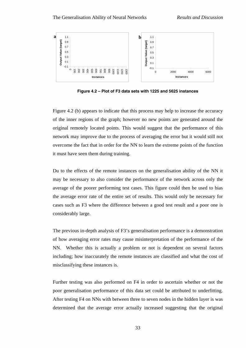
A test was performed to see if it was possible to increase the generalisation
performance of this data set by increasing the grid density of the x and y coordinates
from 35 x 35 to 75 x 75.
32
The Generalisation Ability of Neural Networks Results and Discussion
-0.1
0.1
0.3
0.5
0.7
0.9
1.1
0 100200
300400
500600
700800
9001000
11001200
1300
Instances
Out
put V
alue
(tar
get)
-0.1
0.1
0.3
0.5
0.7
0.9
1.1
0 2000 4000 6000
Instances
Out
put V
alue
(tar
get)
a b
Figure 4.2 – Plot of F3 data sets with 1225 and 5625 instances
Figure 4.2 (b) appears to indicate that this process may help to increase the accuracy
of the inner regions of the graph; however no new points are generated around the
original remotely located points. This would suggest that the performance of this
network may improve due to the process of averaging the error but it would still not
overcome the fact that in order for the NN to learn the extreme points of the function
it must have seen them during training.
Du to the effects of the remote instances on the generalisation ability of the NN it
may be necessary to also consider the performance of the network across only the
average of the poorer performing test cases. This figure could then be used to bias
the average error rate of the entire set of results. This would only be necessary for
cases such as F3 where the difference between a good test result and a poor one is
considerably large.
The previous in-depth analysis of F3’s generalisation performance is a demonstration
of how averaging error rates may cause misinterpretation of the performance of the
NN. Whether this is actually a problem or not is dependent on several factors
including; how inaccurately the remote instances are classified and what the cost of
misclassifying these instances is.
Further testing was also performed on F4 in order to ascertain whether or not the
poor generalisation performance of this data set could be attributed to underfitting.
After testing F4 on NNs with between three to seven nodes in the hidden layer is was
determined that the average error actually increased suggesting that the original
33
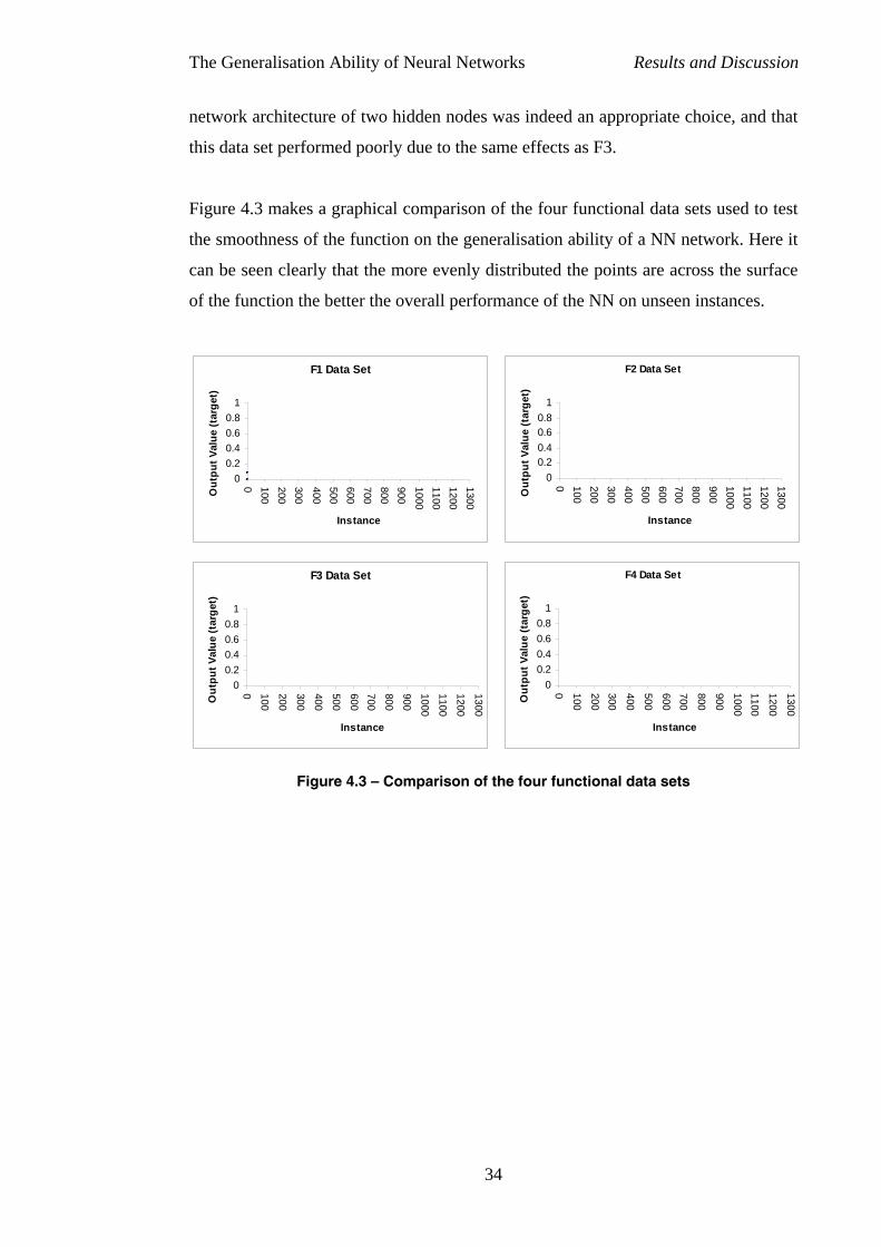
The Generalisation Ability of Neural Networks Results and Discussion
network architecture of two hidden nodes was indeed an appropriate choice, and that
this data set performed poorly due to the same effects as F3.
Figure 4.3 makes a graphical comparison of the four functional data sets used to test
the smoothness of the function on the generalisation ability of a NN network. Here it
can be seen clearly that the more evenly distributed the points are across the surface
of the function the better the overall performance of the NN on unseen instances.
F1 Data Set
00.20.40.60.8
1
0 100200300
400500600700800900
1000110012001300
Instance
Out
put V
alue
(tar
get)
F2 Data Set
00.20.40.60.8
1
0 1002003004005006007008009001000110012001300
InstanceO
utpu
t Val
ue (t
arge
t)
F3 Data Set
00.20.40.60.8
1
0 100
200
300
400
500
600700
800
900
1000
1100
1200
1300
Instance
Out
put V
alue
(tar
get)
F4 Data Set
00.20.40.60.8
1
0 100
200300
400
500
600700
800
900
10001100
1200
1300
Instance
Out
put V
alue
(tar
get)
Figure 4.3 – Comparison of the four functional data sets
34
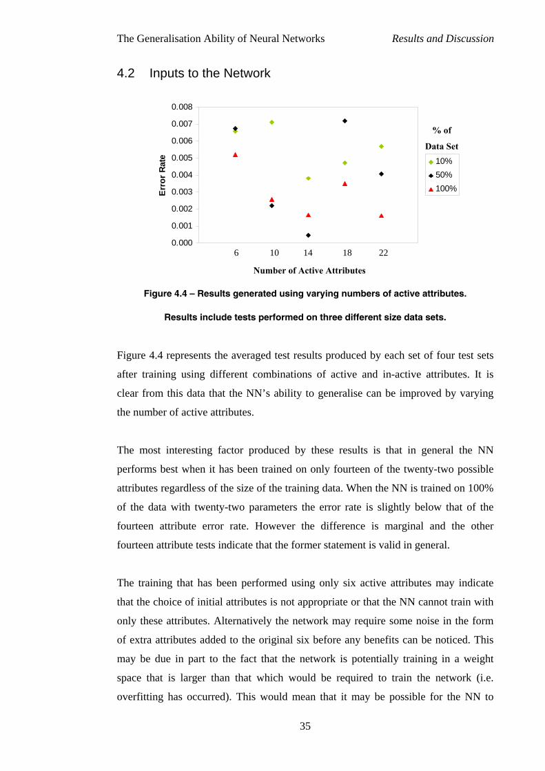
The Generalisation Ability of Neural Networks Results and Discussion
4.2 Inputs to the Network
0.000
0.001
0.002
0.003
0.004
0.005
0.006
0.007
0.008
Erro
r Rat
e 10%50%100%
% of
Data Set
2
Figure 4.4 – R
Results i
Figure 4.4 represen
after training using
clear from this data
the number of activ
The most interesti
performs best when
attributes regardles
of the data with tw
fourteen attribute
fourteen attribute te
The training that h
that the choice of in
only these attribute
of extra attributes a
may be due in par
space that is large
overfitting has occ
6 10 14 18 2
s
esults gen
nclude tes
ts the ave
different
that the N
e attribute
ng factor
it has be
s of the siz
enty-two
error rate.
sts indicat
as been p
itial attrib
s. Alterna
dded to th
t to the fa
r than tha
urred). Th
Active AttributesNumber of Active Attribute
erated using varying numbers of active attributes.
ts performed on three different size data sets.
raged test results produced by each set of four test sets
combinations of active and in-active attributes. It is
N’s ability to generalise can be improved by varying
s.
produced by these results is that in general the NN
en trained on only fourteen of the twenty-two possible
e of the training data. When the NN is trained on 100%
parameters the error rate is slightly below that of the
However the difference is marginal and the other
e that the former statement is valid in general.
erformed using only six active attributes may indicate
utes is not appropriate or that the NN cannot train with
tively the network may require some noise in the form
e original six before any benefits can be noticed. This
ct that the network is potentially training in a weight
t which would be required to train the network (i.e.
is would mean that it may be possible for the NN to
35
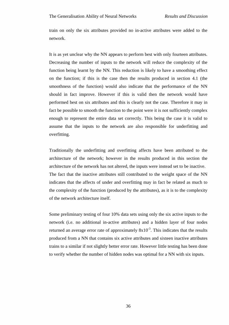
The Generalisation Ability of Neural Networks Results and Discussion
train on only the six attributes provided no in-active attributes were added to the
network.
It is as yet unclear why the NN appears to perform best with only fourteen attributes.
Decreasing the number of inputs to the network will reduce the complexity of the
function being learnt by the NN. This reduction is likely to have a smoothing effect
on the function; if this is the case then the results produced in section 4.1 (the
smoothness of the function) would also indicate that the performance of the NN
should in fact improve. However if this is valid then the network would have
performed best on six attributes and this is clearly not the case. Therefore it may in
fact be possible to smooth the function to the point were it is not sufficiently complex
enough to represent the entire data set correctly. This being the case it is valid to
assume that the inputs to the network are also responsible for underfitting and
overfitting.
Traditionally the underfitting and overfitting affects have been attributed to the
architecture of the network; however in the results produced in this section the
architecture of the network has not altered, the inputs were instead set to be inactive.
The fact that the inactive attributes still contributed to the weight space of the NN
indicates that the affects of under and overfitting may in fact be related as much to
the complexity of the function (produced by the attributes), as it is to the complexity
of the network architecture itself.
Some preliminary testing of four 10% data sets using only the six active inputs to the
network (i.e. no additional in-active attributes) and a hidden layer of four nodes
returned an average error rate of approximately 8x10⁻³. This indicates that the results
produced from a NN that contains six active attributes and sixteen inactive attributes
trains to a similar if not slightly better error rate. However little testing has been done
to verify whether the number of hidden nodes was optimal for a NN with six inputs.
36
The Generalisation Ability of Neural Networks Results and Discussion
4.3 Training Data Size
The results in Figure 4.5 represent the effect the size of the training set has on the
generalisation ability of the NN. It is clear from the result that as the size of the
training set increases so to does the accuracy of the NN. A discussion of several of
the likely reasons as to why this increase in accuracy might occur follows.
0.00
0.000001
0.000010
0.000100
0.001000
0.010000
0.100000
1.000000
Erro
r Rat
e
Figure 4.5 – Av
The first aspec
network archite
performed using
the smaller data
NN itself that w
As a result of
confirm whethe
NN with betwee
to the results of
same 10% data
results (see Figu
0000 10 25 50 75 100
Percentage of Data Set
erage error rate produced from testing of varying percentage sizes of
the mushroom data set
t that must be considered when evaluating these results is that the
cture was not altered during the training process (i.e. all tests were
a hidden layer of eight nodes). This gives rise to the possibility that
sets are suffering from overfitting. If this was the case then it is the
as performing poorly rather than the training data itself.
the obvious downward trend in Figure 4.5 it became necessary to
r or not overfitting was occurring. This was achieved by training the
n three and seven nodes in the hidden layer and comparing this result
the eight node network. The training process was performed on the
sets as the original training to ensure maximum compatibility of
re 4.6).
37
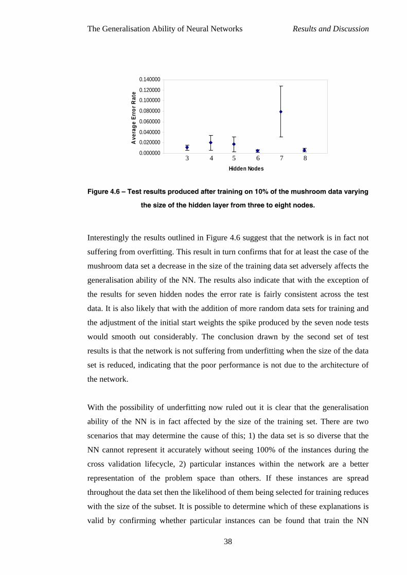
The Generalisation Ability of Neural Networks Results and Discussion
0.000000
0.020000
0.040000
0.060000
0.080000
0.100000
0.120000
0.140000
Hidden Nodes
Ave
rage
Err
or R
ate
3 4 5 6 7 8
Figure 4.6 – Test results produced after training on 10% of the mushroom data varying
the size of the hidden layer from three to eight nodes.
Interestingly the results outlined in Figure 4.6 suggest that the network is in fact not
suffering from overfitting. This result in turn confirms that for at least the case of the
mushroom data set a decrease in the size of the training data set adversely affects the
generalisation ability of the NN. The results also indicate that with the exception of
the results for seven hidden nodes the error rate is fairly consistent across the test
data. It is also likely that with the addition of more random data sets for training and
the adjustment of the initial start weights the spike produced by the seven node tests
would smooth out considerably. The conclusion drawn by the second set of test
results is that the network is not suffering from underfitting when the size of the data
set is reduced, indicating that the poor performance is not due to the architecture of
the network.
With the possibility of underfitting now ruled out it is clear that the generalisation
ability of the NN is in fact affected by the size of the training set. There are two
scenarios that may determine the cause of this; 1) the data set is so diverse that the
NN cannot represent it accurately without seeing 100% of the instances during the
cross validation lifecycle, 2) particular instances within the network are a better
representation of the problem space than others. If these instances are spread
throughout the data set then the likelihood of them being selected for training reduces
with the size of the subset. It is possible to determine which of these explanations is
valid by confirming whether particular instances can be found that train the NN
38
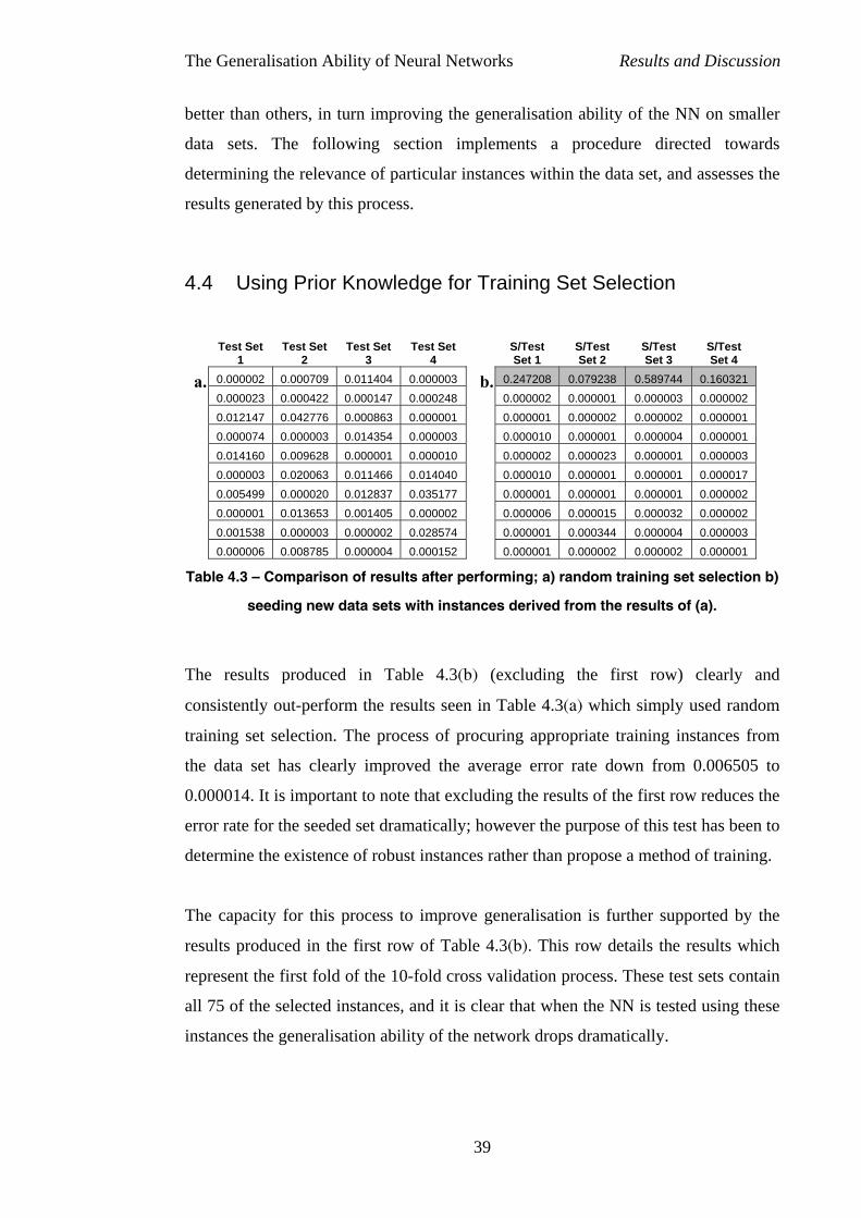
The Generalisation Ability of Neural Networks Results and Discussion
better than others, in turn improving the generalisation ability of the NN on smaller
data sets. The following section implements a procedure directed towards
determining the relevance of particular instances within the data set, and assesses the
results generated by this process.
4.4 Using Prior Knowledge for Training Set Selection
Test Set
1 Test Set
2 Test Set
3 Test Set
4 S/Test
Set 1 S/Test Set 2
S/Test Set 3
S/Test Set 4
0.000002 0.000709 0.011404 0.000003 0.247208 0.079238 0.589744 0.160321 0.000023 0.000422 0.000147 0.000248 0.012147 0.042776 0.000863 0.000001 0.000074 0.000003 0.014354 0.000003 0.014160 0.009628 0.000001 0.000010 0.000003 0.020063 0.011466 0.014040 0.005499 0.000020 0.012837 0.035177 0.000001 0.013653 0.001405 0.000002 0.001538 0.000003 0.000002 0.028574 0.000006 0.008785 0.000004 0.000152
.
Table 4.3 – Comparison of results after pe
seeding new data sets with insta
The results produced in Table 4.3(b
consistently out-perform the results seen
training set selection. The process of pr
the data set has clearly improved the a
0.000014. It is important to note that excl
error rate for the seeded set dramatically;
determine the existence of robust instance
The capacity for this process to improve
results produced in the first row of Tabl
represent the first fold of the 10-fold cros
all 75 of the selected instances, and it is
instances the generalisation ability of the
b
a. 0.000002 0.000001 0.000003 0.000002 0.000001 0.000002 0.000002 0.000001 0.000010 0.000001 0.000004 0.000001 0.000002 0.000023 0.000001 0.000003 0.000010 0.000001 0.000001 0.000017 0.000001 0.000001 0.000001 0.000002 0.000006 0.000015 0.000032 0.000002 0.000001 0.000344 0.000004 0.000003 0.000001 0.000002 0.000002 0.000001rforming; a) random training set selection b)
nces derived from the results of (a).
) (excluding the first row) clearly and
in Table 4.3(a) which simply used random
ocuring appropriate training instances from
verage error rate down from 0.006505 to
uding the results of the first row reduces the
however the purpose of this test has been to
s rather than propose a method of training.
generalisation is further supported by the
e 4.3(b). This row details the results which
s validation process. These test sets contain
clear that when the NN is tested using these
network drops dramatically.
39
The Generalisation Ability of Neural Networks Results and Discussion
One of many questions that arise from these results is; can the NN be trained using
only the selected instances? Preliminary testing indicates that performing inverse 10-
fold cross validation11 does not work using 10% of the data. However, after
introducing an extra one hundred random instances to the training data the network
performed quite well producing an error-rate in the order of 10-7. This same network
was also tested using approximately 7000 instances and produced results in the order
of 10-6. It is possible that the extra 100 instances simply helped reduce the effects of
over fitting by adding some noise to the data set in the form of weaker instances.
One drawback of this approach is that in order to produce a set of optimal instances it
is first necessary to train the NN on randomly selected data sets. As a result of this
the process devised in this section may not be appropriate on a larger scale. It has
served the purpose of proving that data sets contain instances of varying relevance. It
signifies that if it is possible to determine which training instances are best then the
generalisation ability of a NN can be improved when only small data sets are
available.
Time constraints have not allowed further testing to be carried out to confirm the
validity of these results. However it would seem that the 75 original instances
selected for the training process are a robust representation of the data set. Section
6.7 discusses key issues that require investigation within this particular domain.
11 One tenth of data used for training, Nine tenths for testing.
40
The Generalisation Ability of Neural Networks Conclusions
5 Conclusions
After extensive testing it is clear that smoothness of the function, inputs to the NN,
training data selection, and prior knowledge all affect the generalisation ability of
NNs.
The beginning of section 3.3 discusses the relationship between the error rate and the
actual accuracy of the network. It suggests that even when the error rate for the
mushroom data set is at its poorest, applying a threshold to the output will still
produce 100% accuracy. When this is related back to the results produced it is often
the case that even when the generalisation performance of the NN is at its worst it is
still considerably accurate. It is therefore important to re-iterate that the research
performed throughout this thesis has been on examining the affects the five key areas
have on the generalisation ability of NNs not merely whether it is possible to train a
network to classify to 100% accuracy.
It is also very important to note that although the network has at times performed at
100% accuracy the techniques used to achieve this may not work on other data sets.
Because of this the methodology and results provided within this document should
only serve as a platform for which further testing should be performed using different
data sets and increasing the number of tests performed (see section 6 for more
details).
5.1 Function Smoothness
The creation and testing of four artificial functional data sets has clearly
demonstrated that as the smoothness of the function decreases so too does the
generalisation ability of the NN. Moreover the network’s ability to generalise on
functions of a discontinuous nature is much lower than that of continuous functions.
Alternatively, the F3 data set also demonstrated that it may not be immediately
obvious that the NN network is performing badly. A misleadingly good error rate
41
The Generalisation Ability of Neural Networks Conclusions
was reported during testing due to the averaging process across the 10 folds of the
cross validation process. Which lead to F3’s results performing better than F2’s.
On closer inspection it was clear that this was due to fact that the F3 data set
contained a small number of important instances that were often not represented in
the test set. When this occurred, the NN performed very well, due mainly to the fact
that it was classifying instances on a relatively smooth plane. When these instances
did exist in the test set, the impact on the networks ability to generalise was severely
reduced.
The results produced by F3 and F4 were based on artificial data sets so that it was
possible to visually comprehend the smoothness of the function. It may be possible
to use these data sets and others like it to generate an algorithm capable of
determining how smooth the function being learned by a NN is. Algorithms such as
these could then be applied to the n-dimensional hyper-planes produced by real
world data sets; section 6.3 discusses this topic in detail.
5.2 Inputs to the Network
The tests related to the affect the inputs to a NN have on the generalisation ability of
the network, produced evidence suggesting that a larger number of attributes will not
necessarily perform better than a smaller number of attributes. It was seen in these
results that fourteen active attributes actually produced, on average, better results
than twenty-two active attributes.
The conclusion drawn by these results suggests that reducing the number of active
attributes has the affect of smoothing the function that is learnt by the NN. This in
turn is not unlike the traditional problem of underfitting and overfitting and that
altering the number of active attributes to the network has a similar affect to altering
the actual size of the network itself.
42
The Generalisation Ability of Neural Networks Conclusions
5.3 Training Data Size
The results produced in section 4.3 indicate that altering the size of the data set used
to train a NN has an obvious impact on the generalisation ability, and that the larger
the data set is the better the network performs. It was proposed that this occurred for
one of two reasons; 1) the network was suffering from overfitting when training on
small data sets or 2) or that the NN was really being affected by the size of the data.
After performing a set of comprehensive tests it was determined that the NN was in
fact not suffering from the affects of overfitting and that it was in fact the case that
the small size of the data sets was causing the network to perform poorly.
As a result of this finding it was decided that the NNs performance on small data sets
could be attributed to one of two possibilities: 1) the data set is so diverse that the
NN cannot represent it accurately without seeing 100% of the instances during the
cross validation lifecycle, 2) particular instances within the network are a better
representation of the problem space than others, and if these instances are spread
throughout the data set then the likelihood of them being selected for training is
proportionate to the size of the subset.
In order to find a solution to this problem it was necessary to first derive a means of
determining whether the data set did in fact possess training instances that produced
better results than other instances within the set. If it were the case that no particular
instances out-performed other instances then it would be necessary to increase the
size of the data set in order to improve generalisation. However if particular
instances could be singled out as being optimal, the NN could potentially be trained
on a small set of these optimal training instances.
In order to answer this question the prior knowledge was used as a method of
selecting an optimal training set and the results prove that it is in fact possible to
build a small training of set optimal instances capable of generalising well on large
test sets. A further discussion of these results is included in the following section and
also in section 4.4.
43
The Generalisation Ability of Neural Networks Conclusions
5.4 Using Prior Knowledge to Select Training Data
This section determines whether optimal instances existed within a data set by
analysing the results from section 4.3 and identifies instances where a particular fold
of the test set performed poorly. The output files for these test runs were then
examined to determine which instances within the data set performed the worst
during testing. These instances were then combined with a selection of random data
in an effort to produce a small yet highly optimal training set.
The results clearly demonstrated that it was in fact possible to identify instances of
optimal performance within a data set. However the process used to derive these
instances from the original data set required previous results produced by the NN,
resulting in an increase in the number of times the NN must be trained before a good
generaliser is produced.
The extra overhead required to implement this selection process is a potential
deterrent for its implementation in large scale problems however in proving that
optimal instances do in fact exist it provides a solid basis for further research into
finding faster methods of determining the optimal instances within a training set.
44

The Generalisation Ability of Neural Networks Further Work
6 Further Work
6.1 Retesting on Different Data Sets
The training and testing performed throughout this research was carried out on a
limited number of data sets. With the exception of the functional data sets used to
test the effects of the smoothness of the function on the generalisation ability, the
mushroom data set has been used for all training and testing.
The mushroom data set has proven to be useful due to its size and complexity
however even a brief look at the other data sets contained within the UCI’s
repository will highlight the fact that there are a vast number of differing types of
data sets. The differences include missing values, the number of attributes, the
number of instances and whether the output is nominal or continuous.
The shear vastness of these differences indicates that the work carried out within this
research should only serve as a benchmark and that the training and testing
performed on the mushroom data set should be tested on other data sets within the
UCI’s repository. Only then would it be possible to draw any conclusions about the
results produced throughout this research.
6.2 Retesting Using More Random Subsets
In addition to performing the tests outlined in the section 6.1 it will also be necessary
to increase the number of subsets selected from each data set to something much
larger. When random subsets were selected from the mushroom data set this was
capped at a maximum of four subsets per test due to time and equipment constraints.
As a result when only 10% of the data set was selected randomly, it is only possible
that at most 40% of the actual data set was selected. Because the subsets were
randomly selected from the entire data set each time, it is likely that this figure is
even lower as some instances will have undoubtedly been selected for more than one
of the four subsets.
45
The Generalisation Ability of Neural Networks Further Work
In determining the number of subsets to select it is proposed that the following
method be used; the number of subsets multiplied by the number of instances within
a given subset12 should be no less than one and a half times the total number of
instances within the original data set. Therefore in the case of the 10% subset
selection for the mushroom data no less than fifteen subsets should be randomly
selected for training and testing. As a result the subsets will better represent the
original data set and allow for a higher precision of results to be produced.
6.3 Determining the Smoothness of a Function
The results produced within section 4.1 clearly indicate that the smoothness of the
function being learned by a NN affects the generalisation ability of the network
during the testing of unseen data. The process used to determine this affect was to
create data sets of varying smoothness and analyse the results from each. The
dilemma of this process is that it is not possible to determine the smoothness of real
data sets due to their multi-dimensional nature.
This research should therefore be extended into a secondary stage whereby a means
of determining how discontinuous the function being learnt is, based on the changes
occurring within the weights of the network. This process would likely involve
monitoring the rate of change of individual weights within the network and may
result in calculating some measure during training that indicates how smooth the
function being learnt is.
6.3.1 Smoothing Discontinuous Functions
If a satisfactory method of determining the smoothness of the function is created then
it would be possible to transfer the testing over to real data sets. The results in section
4.2 suggest that it may in fact be possible to smooth the function generated by a data
set and therefore produce better generalisation. Having a means of measuring the
smoothness of an unknown function would allow this to be verified.
12 Each subset group should contain the same number of instances.
46
The Generalisation Ability of Neural Networks Further Work
Tests similar to those performed previously in section 3.6 could be re-run and the
smoothness of the function generated by the different combinations of active and
inactive inputs could be evaluated. If this testing produced results that confirm that
the smoothness of the function is altered by the inputs to the network then it is
possible to determine the optimal set of inputs to the network.
6.4 Determining Optimal Attributes
The results produced in section 4.2 indicate that some attributes are more suited to
training a neural network than others. However in order to ascertain which attributes
provide the best generalisation performance during testing it is necessary to try
arbitrary combinations of attributes, which inevitably consumes time and resources.
It is possible that a faster method for determining optimal attributes exists. The
analysis of optimal and sub-optimal attributes selected during the processes
described in section 3.6 could be carried out. The results of this analysis could then
be used to produce an algorithm that can be applied to the attributes in a data set in
order to select the optimal attributes for training. Therefore training of the NN would
only be done once a set of optimal attributes have been selected resulting in a
considerable reduction in costs.
6.5 Variations in Neural Network Architecture
Further testing should be performed to ascertain how deactivating the inputs to a NN
compares to actually removing the inputs. This would help to prove or disprove the
suggestions made in section 3.6 regarding whether or not the affects of underfitting
and overfitting could be reduced by selecting an optimal set of attributes from the
class rather than altering the size of the network.
6.6 Continuous and Discrete Attribute Performance
Most of the testing performed within this research was performed on the mushroom
data set, which contains twenty-two discrete attributes. It is therefore proposed that
testing of the processes in sections 3.5, 3.6 and 3.8 should therefore be carried out on
47
The Generalisation Ability of Neural Networks Further Work
data sets with only continuous attributes and also a mix of continuous and discrete
attributes.
6.7 Finding Optimal Instances
The results produced in section 4.4 clearly indicate that it is in fact possible to create
a small set of optimal instances capable of accurately classifying a larger set of test
data. The question that arises from these results is; what makes some instances better
than others?
Further work should therefore approach this topic in an effort to determine whether
this appears to occur simply because many of the instances are similar and therefore
have little affect on the training process. If this is the case, the direction taken from
this point should be towards finding a means of reducing a data set down to a set of
unique instances capable of out performing the entire data set. If not, work should be
carried out in order to determine what makes it possible that a small set of optimal
instances are capable of representing many other apparently unique instances.
6.7.1 The Number of Optimal Instances
In addition to the work mentioned above, testing should also be carried out to
determine what ratio of optimal instances is required to successfully train a NN. This
is an important aspect, as reducing the size of the training set has the positive affect
of increasing the size of the test set. If the NN can be tested on more instances and
still perform as well as traditional 10-fold cross validation techniques then the
network would be expected to be even more reliable than that of its 10-fold
counterpart.
6.8 Missing and Noisy Data
Aside from choosing to treat the missing values within the mushroom data set as
another possible value no testing has been performed with the intention of
determining the effects of missing or noisy data. The occurrence of these two factors
is common in real world data sets and should therefore be incorporated into further
testing.
48
The Generalisation Ability of Neural Networks References
7 References
Abu-Mostafa, Y. S. (1990). "Learning from hints in Neural Networks." Journal of Complexity 6: 192-198. Aran, O. and E. Alpaydin (2003). An Incremental Neural Network Construction Algorithm for Training Multilayer Perceptrons. International Conference of Artificial Neural Networks ICANN. Atiya, A. and C. Ji (1997). "How Initial Conditions Affect Generalization Performance in Large Networks." IEEE Transactions on Neural Networks 8(2): 448-451. Bishop, C. M. (1995). Neural networks for pattern recognition, Oxford University Press, NY. Bishop, C. M. (1995). "Training with Noise is Equivalent to Tikonov Regularization." Neural Computation 7(1): pp. 108-116. Burrascano, P. (1992). Network topology, traning set size, and generalization ability in MLP's project. Artificial Neural Networks, Brighton, Elsevier Science Publishers B.V. Cameron-Jones, M. (2004). Personal Communication. R. Fearn. University of Tasmania. Chakraborty, D. and N. R. Pal (2003). "A Novel Training Scheme for Multilayered Perceptrons to Realize Proper Generalization and Incremental Learning." IEEE Transactions on Neural Networks 14(1): pp. 1-14. Christiansen, M. H. (1998). Improving Learning and Generalization in Neural Networks through the Acquisition of Multiple Related Functions. Proceedings of the Fourth Neural Computation and Psychology Workshop: Connectionist Representations, London, Springer-Verlag. Davalo, E. and P. Naim (1992). Neural Networks, The Macmillan Press Ltd. Dayhoff, J. (1990). Neural Network Architectures - An Introduction, Thomas Nelson Australia. Duch, W. and R. Adamczak (1998). Statistical methods for consruction of neural networks. International Conference on Neural Information Processing, Kitakyushu, Japan. Duch, W. and K. Grabczewski (1999). Searching for optimal MLP. 4th Conference on Neural Networks and Their Applications, Zakopane, pp. 65-70.
49
The Generalisation Ability of Neural Networks References
Duch, W. and M. Kordos (2004). On Some Factors Influencing MLP Error Surface. 7th International Conference on Artificial Intelligence and Soft Computing, Zakopane, Poland, Lecture Notes in AI Vol. 3070; pp. 217-222. F. M. Richardson et al (Date Unknown). The Influence of Prior Knowledge and Related Experience on Generalisation Performance in Connectionist Networks. Franklin, D. (2003). Selection and Preparation of Training Data, http://ieee.uow.edu.au/~daniel/software/libneural/BPN_tutorial/BPN_English/BPN_English/node9.html. 2004. Galkin, I. (2002). Crash Introduction to Artificial Neural Networks, http://ulcar.uml.edu/~iag/CS/Intro-to-ANN.html. 2004. Geman S et al (1992). "Neural networks and the bias/variance dilemma." Neural Computation 4: 1-58. Haykin, S. (1994). Neural Networks - A Comprehensive Foundation, Maxwell Macmillan International. Hebb, D. (1949). The Organization of Behaviour: A Neuropsychological Theory, John Wiley &Sons. Hornik, K. (1991). "Approximation Capabailities of Multilayer Feedforward Networks." Neural Networks 4: 251-257. Hornik, K. (1993). "Some New Results on Neural Network Approximation." Neural Networks 6: 1069-1072. Leshno, M., V. Y. Lin, et al. (1993). "Multilayer Feedforward Network with Non-Polynomial Activation Function can Aproximate Any Function." Neural Networks 6: 861-867. McCulloch, W. S. and W. H. Pitt (1943). "A logical calculus of the ideas immanent in nervous activity, Bulletin of Mathematical Biophysics, 5: pp.115-133." Messer, M. and J. Kittler (1998). Choosing the Optimal Neural Network Size to Aid a Search through a Large Image Database, University of Surrey Guildford, Surrey. Minsky, M. and S. Papert (1968). Perceptrons: an Introduction to Computational Geometry., MIT Press. Mitchell, T. M. (1997). Machine Learning, McGraw Hill. Parker, D. (1982). Learning Logic, Invention Report. Stanford, CA, Stanford University: pp. 581-64. Quinlan, R. (1983). Learning Efficient Classification Procedures and their Application to Chess and Games. Machine Learning. An Artificial Intelligence Approach, pp. 463-482.
50
The Generalisation Ability of Neural Networks References
Rosenblatt, F. (1958). "The Perceptron: A Probabilistic Model for Information Storage and Organization in the Brain." Cornell Aeronautical Laboratory, Psychological Review 65(6): pp. 386-408. Rumelhart, D. E. and J. L. McClelland (1986). Parallel Distributed Processing: Explorations in the Microstructure of Cognition, Volumes 1 and 2. Cambridge, MA, MIT Press. S C Suddarth Y L Kergosien (1991). Rule-injection hints as a means of improving network performance and learning time. Proceedings of the Networks/EURIP Workshop 1990, Berlin, Springer-Verlag. S Lawrence et al (1996). "What Size Neural Network Gives Optimal Generalization? Convergence Properties of Backpropagation." Sarkar, D. (1996). "Randomness in Generalization Ability: A Source to Improve It." IEEE Transactions on Neural Networks 7(3): 676-685. Sarle, W. S. (1995). Stopped Training and Other Remedies for Overfitting. Proceedings of the 27th Symposium on the Interface of Computing Science and Statistics, Pittsburgh, PA, 27: pp. 352 - 360. Schmidt, W. F., S. Raudys, et al. (1993). Initialization, back-propagation and generalization of feed-forward classifiers. Proceedings of the IEEE International Conference on Neural Networks, ICNN-93. Schneider, J. (1997). Cross Validation, site viewed 9/5/2004, http://www-2.cs.cmu.edu/~schneide/tut5/node42.html. Schoner, W. (1992). Reaching the Generalization Maximum of Backpropagation Networks. Artificial Neural Networks, Brighton, Elsevier Science Publishers B.V. Swingler, K. (1996). Applying Neural Networks - A Practical Guide, Academic Press. Tamburini, F. and R. Davoli (1994). An Algorithmic method to build good training sets for neural-network classifiers. Bolgna, University of Bologna (Italy). Ting, K. M. and I. H. Witten (1997). Stacked Generalization: when does it work? International Joint Conference on Artificial Intelligence, Nagoya, Japan. V Tresp et al (1994). Training Neural Networks with Deficient Data. Advances in Nerual Information Processing Systems 6, San Mateo, CA, Morgan Kauffman. W S Sarle et al (2002). Neural Network FAQ, site viewed 31/3/2004, ftp://ftp.sas.com/pub/neural/FAQ.html. Werbos, P. J. (1974). Beyond regression: New tools for prediction and analysis in the behavioral sciences. Cambridge, MA, Harvard University.
51

The Generalisation Ability of Neural Networks References
Witten, I. H. and E. Frank (2000). Data Mining: Practical machine learning tools with Java implementations. San Francisco, CA, Morgan Kaufmann. Wolpert, D. (1992). "Stacked Generalization." Neural Networks 5: 241-259. Young, M. E. (2003). A Brief History of Connectionism and Information Processing. 2004: Lecture.
52
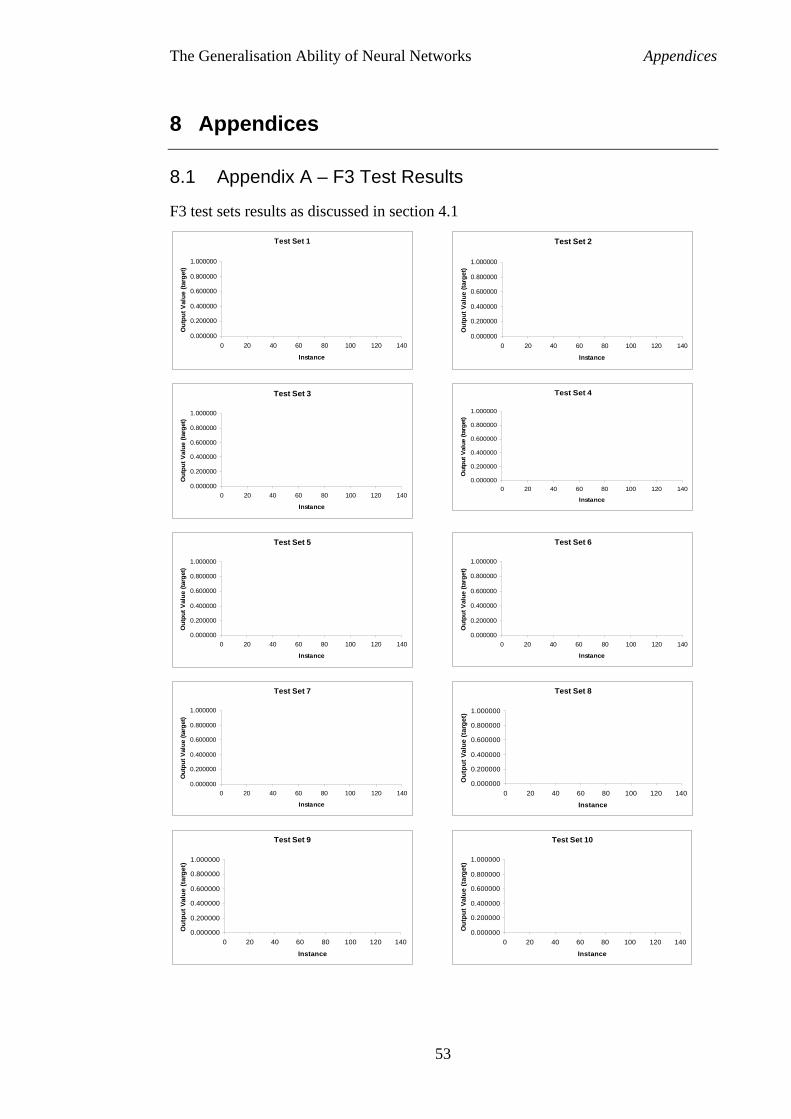
The Generalisation Ability of Neural Networks Appendices
8 Appendices
8.1 Appendix A – F3 Test Results
F3 test sets results as discussed in section 4.1
Test Set 1
0.000000
0.200000
0.400000
0.600000
0.800000
1.000000
0 20 40 60 80 100 120 140
Instance
Out
put V
alue
(tar
get)
Test Set 2
0.000000
0.200000
0.400000
0.600000
0.800000
1.000000
0 20 40 60 80 100 120 140
Instance
Out
put V
alue
(tar
get)
Test Set 3
0.000000
0.200000
0.400000
0.600000
0.800000
1.000000
0 20 40 60 80 100 120 140
Instance
Out
put V
alue
(tar
get)
Test Set 4
0.000000
0.200000
0.400000
0.600000
0.800000
1.000000
0 20 40 60 80 100 120 140
Instance
Out
put V
alue
(tar
get)
Test Set 5
0.000000
0.200000
0.400000
0.600000
0.800000
1.000000
0 20 40 60 80 100 120 140
Instance
Out
put V
alue
(tar
get)
Test Set 6
0.000000
0.200000
0.400000
0.600000
0.800000
1.000000
0 20 40 60 80 100 120 140
Instance
Out
put V
alue
(tar
get)
Test Set 7
0.000000
0.200000
0.400000
0.600000
0.800000
1.000000
0 20 40 60 80 100 120 140
Instance
Out
put V
alue
(tar
get)
Test Set 8
0.000000
0.200000
0.400000
0.600000
0.800000
1.000000
0 20 40 60 80 100 120 140
Instance
Out
put V
alue
(tar
get)
Test Set 9
0.000000
0.200000
0.400000
0.600000
0.800000
1.000000
0 20 40 60 80 100 120 140
Instance
Out
put V
alue
(tar
get)
Test Set 10
0.000000
0.200000
0.400000
0.600000
0.800000
1.000000
0 20 40 60 80 100 120 140
Instance
Out
put V
alue
(tar
get)
53

The Generalisation Ability of Neural Networks Appendices
8.2 Appendix B – Electronic Submission
train.c – The Neural Network training program, this program has undergone many
changes, however the key changes are commented.
test.c – A variation of train.c that does not include any weight adjustments and only
runs for one epoch.
weights.c – The program used to generate random initial weights
thesis.pdf – an electronic copy of this thesis
54