Embed Size (px)
Citation preview
The Gauss-Bonnet TheoremAn Introduction to Index Theory
Gianmarco Molino
SIGMA Seminar
1 Februrary, 2019
Gianmarco Molino (SIGMA Seminar) The Gauss-Bonnet Theorem 1 Februrary, 2019 1 / 23
Topological Manifolds
An n-dimensional topological manifold M is an abstract way ofrepresenting space:
Formally it is a set of points M, a collection of ‘open sets’ T , and aset of continuous bijections of neighborhoods of each point with openballs in Rn called charts.
Topological manifolds don’t really have a sense of ‘distance’; that’sthe key difference between the study of topology and geometry.
Gianmarco Molino (SIGMA Seminar) The Gauss-Bonnet Theorem 1 Februrary, 2019 2 / 23

Topological manifolds
Topological manifolds are considered equivalent (homeomorphic) ifthey can be ‘stretched’ to look like one another without being ‘cut’ or‘glued’.
A homeomorphism is a continuous bijection.
Any property that is invariant under homeomorphisms is considered atopological property.
Gianmarco Molino (SIGMA Seminar) The Gauss-Bonnet Theorem 1 Februrary, 2019 3 / 23
Euler Characteristic
It’s possible to decompose topological manifolds into ‘triangulations’.
In the context of surfaces, this will be a combination of vertices,edges, and faces; in higher dimensions we use higher dimensionalsimplices.
Given a triangulation, we define the constants
bi = #i-simplices
Gianmarco Molino (SIGMA Seminar) The Gauss-Bonnet Theorem 1 Februrary, 2019 4 / 23
Euler Characteristic
We then define the Euler Characteristic of a manifold M with a giventriangulation as
χ =n∑
i=0
(−1)ibi
The Euler characteristic can be shown to be independent of thetriangulation, and is thus a property of the manifold.
It’s moreover invariant under homeomorphism, and even more thanthat it’s invariant under homotopy equivalence.
Gianmarco Molino (SIGMA Seminar) The Gauss-Bonnet Theorem 1 Februrary, 2019 5 / 23
Riemannian Manifolds
We can add to topological manifolds more structure;
A topological manifold equipped with charts that preserve the smoothstructure of Rn are called smooth manifolds.
A smooth manifold equipped with a smoothly varying inner productg(·, ·) on its tangent bundle is called a Riemannian manifold.
Riemannian manifolds have well defined notions of distance andvolume, and can be naturally equipped with a notion of derivative(Levi-Civita connection).
Gianmarco Molino (SIGMA Seminar) The Gauss-Bonnet Theorem 1 Februrary, 2019 6 / 23

Surfaces and Gaussian Curvature
We’ll begin by only considering surfaces, that is Riemannian2-manifolds isometrically embedded in R3, and take an historicalperspective.
Given a smooth curveγ : [0, 1]→M
we can define its curvature
kγ(s) = |γ′′(s)|
This is an extrinsic definition; the derivatives are taken in R3 anddepend on the embedding of M.
Gianmarco Molino (SIGMA Seminar) The Gauss-Bonnet Theorem 1 Februrary, 2019 7 / 23
Surfaces and Gaussian Curvature
For each point x ∈M we consider the collection of all smooth curvespassing through x and define the ‘principal curvatures’
k1 = infγ
(kγ), k2 = supγ
(kγ)
Gauss defined the Gaussian curvature of a surface M to be
K = k1k2
and proved in his famous Theorema Egregium (1827) that it is anintrinisic property; that is it is independent of the embedding.
Gianmarco Molino (SIGMA Seminar) The Gauss-Bonnet Theorem 1 Februrary, 2019 8 / 23
Gauss-Bonnet Theorem
O. Bonnet (1848) showed that for a closed, compact surface M∫MK = 2πχ
This is remarkable, relating a global, topological quantity χ to a local,analytical property K .
Gianmarco Molino (SIGMA Seminar) The Gauss-Bonnet Theorem 1 Februrary, 2019 9 / 23
Proof of the Gauss-Bonnet Theorem
Consider first a triangular region R of a surface.
Using a parameterization (u, v) we can write the curvature in localcoordinates as∫
RK = −
∫∫π−1(R)
((Ev
2√EG
)v
+
(Gu
2√EG
)u
)dudv
Gianmarco Molino (SIGMA Seminar) The Gauss-Bonnet Theorem 1 Februrary, 2019 10 / 23
Proof of the Gauss-Bonnet Theorem
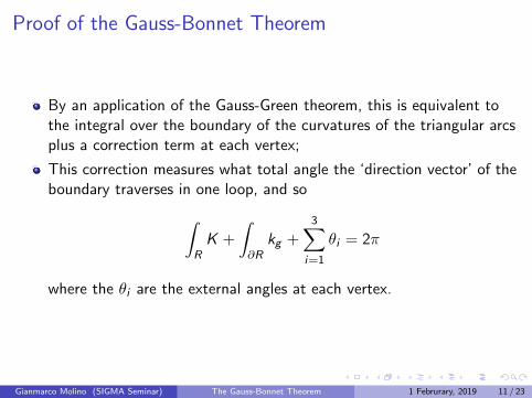
By an application of the Gauss-Green theorem, this is equivalent tothe integral over the boundary of the curvatures of the triangular arcsplus a correction term at each vertex;
This correction measures what total angle the ‘direction vector’ of theboundary traverses in one loop, and so∫
RK +
∫∂R
kg +3∑
i=1
θi = 2π
where the θi are the external angles at each vertex.
Gianmarco Molino (SIGMA Seminar) The Gauss-Bonnet Theorem 1 Februrary, 2019 11 / 23
Proof of the Gauss-Bonnet Theorem
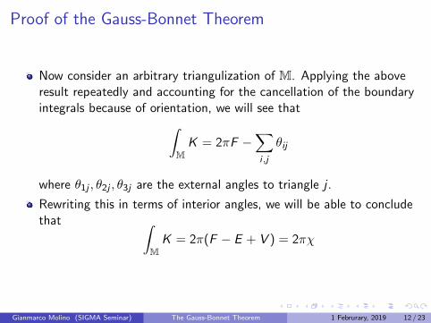
Now consider an arbitrary triangulization of M. Applying the aboveresult repeatedly and accounting for the cancellation of the boundaryintegrals because of orientation, we will see that∫
MK = 2πF −
∑i ,j
θij
where θ1j , θ2j , θ3j are the external angles to triangle j .
Rewriting this in terms of interior angles, we will be able to concludethat ∫
MK = 2π(F − E + V ) = 2πχ
Gianmarco Molino (SIGMA Seminar) The Gauss-Bonnet Theorem 1 Februrary, 2019 12 / 23
Chern-Gauss-Bonnet Theorem
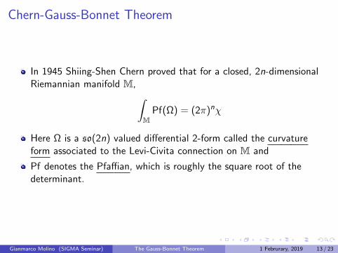
In 1945 Shiing-Shen Chern proved that for a closed, 2n-dimensionalRiemannian manifold M,∫
MPf(Ω) = (2π)nχ
Here Ω is a so(2n) valued differential 2-form called the curvatureform associated to the Levi-Civita connection on M and
Pf denotes the Pfaffian, which is roughly the square root of thedeterminant.
Gianmarco Molino (SIGMA Seminar) The Gauss-Bonnet Theorem 1 Februrary, 2019 13 / 23
Chern-Gauss-Bonnet Theorem
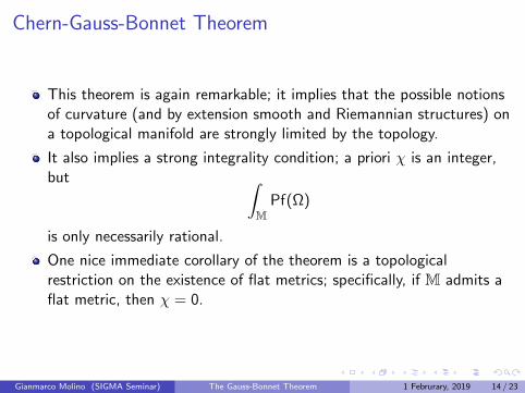
This theorem is again remarkable; it implies that the possible notionsof curvature (and by extension smooth and Riemannian structures) ona topological manifold are strongly limited by the topology.
It also implies a strong integrality condition; a priori χ is an integer,but ∫
MPf(Ω)
is only necessarily rational.
One nice immediate corollary of the theorem is a topologicalrestriction on the existence of flat metrics; specifically, if M admits aflat metric, then χ = 0.
Gianmarco Molino (SIGMA Seminar) The Gauss-Bonnet Theorem 1 Februrary, 2019 14 / 23
Heat kernel proof of the Chern-Gauss-Bonnet Theorem
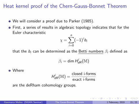
We will consider a proof due to Parker (1985).
First, a series of results in algebraic topology indicates that for theEuler characteristic
χ =n∑
i=0
(−1)ibi
that the bi can be determined as the Betti numbers βi defined as
βi = dimH idR(M)
Where
H idR(M) =
closed i-forms
exact i-forms
are the deRham cohomology groups.
Gianmarco Molino (SIGMA Seminar) The Gauss-Bonnet Theorem 1 Februrary, 2019 15 / 23
Heat kernel proof of the Chern-Gauss-Bonnet Theorem
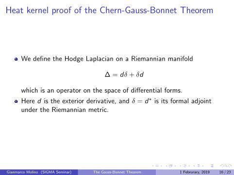
We define the Hodge Laplacian on a Riemannian manifold
∆ = dδ + δd
which is an operator on the space of differential forms.
Here d is the exterior derivative, and δ = d∗ is its formal adjointunder the Riemannian metric.
Gianmarco Molino (SIGMA Seminar) The Gauss-Bonnet Theorem 1 Februrary, 2019 16 / 23
Heat kernel proof of the Chern-Gauss-Bonnet Theorem
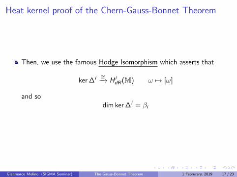
Then, we use the famous Hodge Isomorphism which asserts that
ker ∆i ∼=−→ H idR(M) ω 7→ [ω]
and sodim ker ∆i = βi
Gianmarco Molino (SIGMA Seminar) The Gauss-Bonnet Theorem 1 Februrary, 2019 17 / 23
Heat kernel proof of the Chern-Gauss-Bonnet Theorem
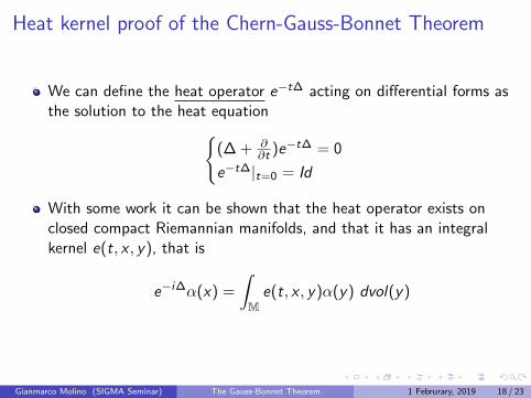
We can define the heat operator e−t∆ acting on differential forms asthe solution to the heat equation
(∆ + ∂∂t )e−t∆ = 0
e−t∆|t=0 = Id
With some work it can be shown that the heat operator exists onclosed compact Riemannian manifolds, and that it has an integralkernel e(t, x , y), that is
e−i∆α(x) =
∫Me(t, x , y)α(y) dvol(y)
Gianmarco Molino (SIGMA Seminar) The Gauss-Bonnet Theorem 1 Februrary, 2019 18 / 23
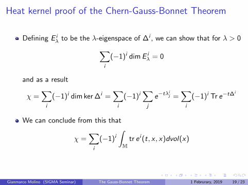
Heat kernel proof of the Chern-Gauss-Bonnet Theorem
Defining E iλ to be the λ-eigenspace of ∆i , we can show that for λ > 0∑
i
(−1)i dimE iλ = 0
and as a result
χ =∑i
(−1)i dim ker ∆i =∑i
(−1)i∑j
e−tλij =
∑i
(−1)i Tr e−t∆i
We can conclude from this that
χ =∑i
(−1)i∫M
tr e i (t, x , x)dvol(x)
Gianmarco Molino (SIGMA Seminar) The Gauss-Bonnet Theorem 1 Februrary, 2019 19 / 23
Heat kernel proof of the Chern-Gauss-Bonnet Theorem
Unfortunately, for most manifolds the computation of the heat kernelis impossible, but we can approximate it using a parametrix (anapproximation close to the diagonal).
Using this approximation and making repeated use of the fact that χis independent of t we will be able to conclude the theorem.
Gianmarco Molino (SIGMA Seminar) The Gauss-Bonnet Theorem 1 Februrary, 2019 20 / 23
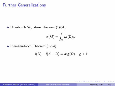
Further Generalizations
Hirzebruch Signature Theorem (1954)
σ(M) =
∫MLk(Ω)4k
Riemann-Roch Theorem (1954)
l(D)− l(K − D) = deg(D)− g + 1
Gianmarco Molino (SIGMA Seminar) The Gauss-Bonnet Theorem 1 Februrary, 2019 21 / 23
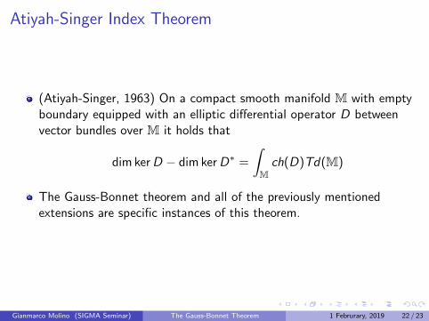
Atiyah-Singer Index Theorem
(Atiyah-Singer, 1963) On a compact smooth manifold M with emptyboundary equipped with an elliptic differential operator D betweenvector bundles over M it holds that
dim kerD − dim kerD∗ =
∫Mch(D)Td(M)
The Gauss-Bonnet theorem and all of the previously mentionedextensions are specific instances of this theorem.
Gianmarco Molino (SIGMA Seminar) The Gauss-Bonnet Theorem 1 Februrary, 2019 22 / 23
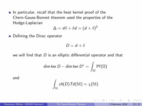
In particular, recall that the heat kernel proof of theChern-Gauss-Bonnet theorem used the properties of theHodge-Laplacian
∆ = dδ + δd = (d + δ)2
Defining the Dirac operator
D = d + δ
we will find that D is an elliptic differential operator and that
dim kerD − dim kerD∗ =
∫M
Pf(Ω)
and ∫Mch(D)Td(M) = χ(M)
Gianmarco Molino (SIGMA Seminar) The Gauss-Bonnet Theorem 1 Februrary, 2019 23 / 23


![DepartmentofMathematics …fold MCMC, Chern-Gauss-Bonnet theorem, Cauchy-Crofton formula, random matrices, real algebraic manifold volume bounds 1 arXiv:1503.03626v1 [math.PR] 12 Mar](https://img.pdfslide.us/doc/110x75/5e7e713e5147e4491976abd4/departmentofmathematics-fold-mcmc-chern-gauss-bonnet-theorem-cauchy-crofton-formula.jpg)


![The Gauss-Bonnet-Chern Theorem on Riemannian …v1ranick/papers/li4.pdfarXiv:1111.4972v4 [math.DG] 28 Nov 2011 The Gauss-Bonnet-Chern Theorem on Riemannian Manifolds Yin Li Abstract](https://img.pdfslide.us/doc/110x75/5e2db7623167111deb2e82ee/the-gauss-bonnet-chern-theorem-on-riemannian-v1ranickpapersli4pdf-arxiv11114972v4.jpg)