Embed Size (px)
Citation preview

The Fundamentals of Heavy TailsProperties, Emergence, & Identification
Jayakrishnan Nair, Adam Wierman, Bert Zwart

Why am I doing a tutorial on heavy tails?
Why are we writing a book on the topic?
Because heavy-tailed phenomena are everywhere!
Because we’re writing a book on the topic…

Why am I doing a tutorial on heavy tails?
Because we’re writing a book on the topic…
Why are we writing a book on the topic?
Because heavy-tailed phenomena are everywhere! BUT, they are extremely misunderstood.

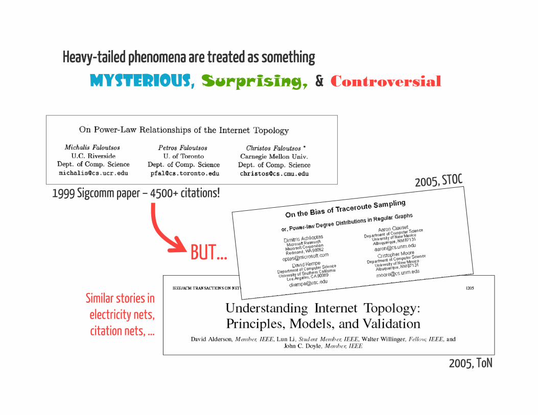
Heavy-tailed phenomena are treated as something
Mysterious, Surprising, & Controversial

Heavy-tailed phenomena are treated as something
Mysterious, Surprising, & Controversial
Our intuition is flawed because intro probability classes focus on light-tailed distributions
Simple, appealing statistical approaches have BIG problems

Heavy-tailed phenomena are treated as something
Mysterious, Surprising, & Controversial
BUT…
2005, ToN
Similar stories in electricity nets, citation nets, …

Heavy-tailed phenomena are treated as something
Mysterious, Surprising, & Controversial
1. Properties 2. Emergence
3. Identification
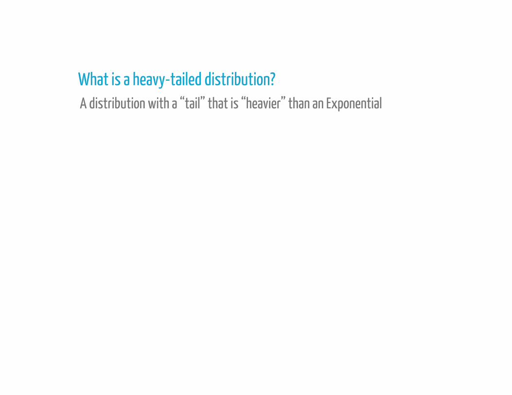
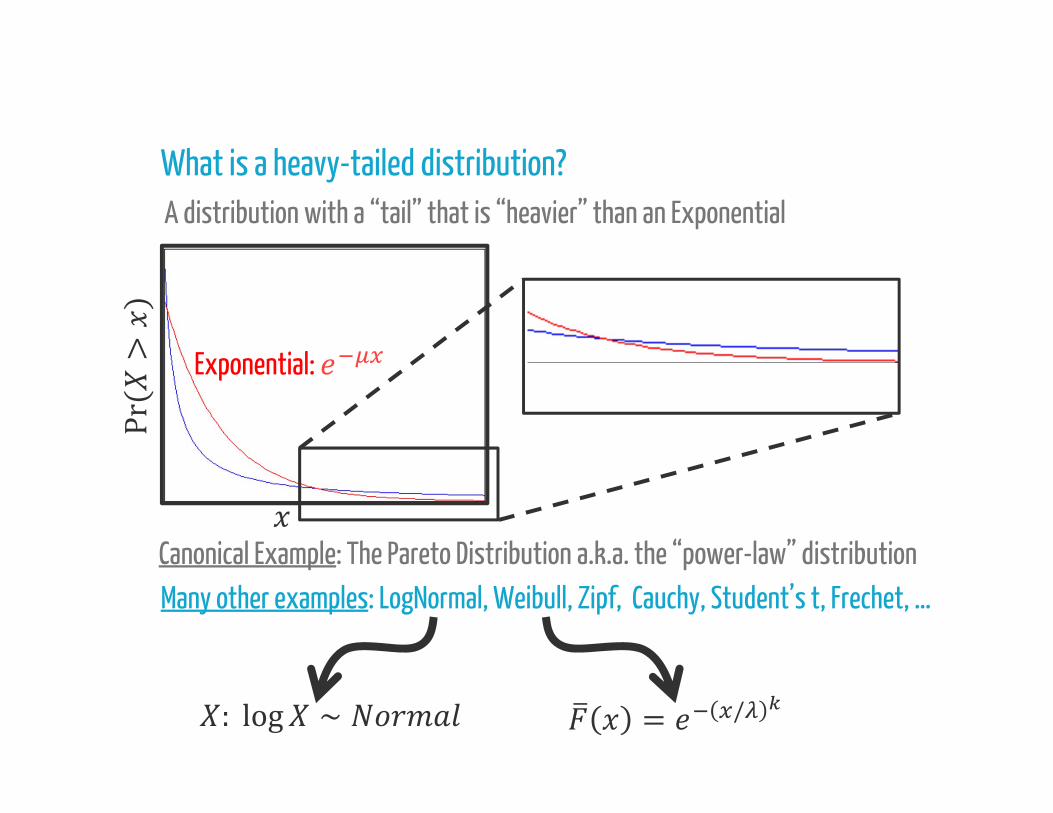
What is a heavy-tailed distribution? A distribution with a “tail” that is “heavier” than an Exponential

What is a heavy-tailed distribution? A distribution with a “tail” that is “heavier” than an Exponential
Exponential: Pr(>)

What is a heavy-tailed distribution?
Canonical Example: The Pareto Distribution a.k.a. the “power-law” distribution
A distribution with a “tail” that is “heavier” than an Exponential
Pr > = ( ) =density: ( ) = for ≥
Exponential: Pr(>)
What is a heavy-tailed distribution? A distribution with a “tail” that is “heavier” than an Exponential
Many other examples: LogNormal, Weibull, Zipf, Cauchy, Student’s t, Frechet, …
: log ∼ = /Canonical Example: The Pareto Distribution a.k.a. the “power-law” distribution
Exponential: Pr(>)

What is a heavy-tailed distribution? A distribution with a “tail” that is “heavier” than an Exponential
Many other examples: LogNormal, Weibull, Zipf, Cauchy, Student’s t, Frechet, …Canonical Example: The Pareto Distribution a.k.a. the “power-law” distribution
Many subclasses: Regularly varying, Subexponential, Long-tailed, Fat-tailed, …
Exponential: Pr(>)

Heavy-tailed distributions have many strange & beautiful properties
• The “Pareto principle”: 80% of the wealth owned by 20% of the population, etc.• Infinite variance or even infinite mean• Events that are much larger than the mean happen “frequently”….
These are driven by 3 “defining” properties1) Scale invariance2) The “catastrophe principle”3) The residual life ”blows up”

Scale invariance

Scale invarianceis scale invariant if there exists an and a such that = ( ) for all , such that ≥ .
“change of scale”

Scale invarianceis scale invariant if there exists an and a such that = ( ) for all , such that ≥ .
Example: Pareto distributions= = 1Theorem: A distribution is scale invariant if and only if it is Pareto.

Scale invarianceis scale invariant if there exists an and a such that = ( ) for all , such that ≥ .
is asymptotically scale invariant if there exists a continuous, finite such that lim→ ( ) = for all .
Asymptotic scale invariance

Example: Regularly varying distributionsis regularly varying if = ( ), where ( ) is slowly varying,
i.e., lim→ ( )( ) = 1 for all > 0.
Theorem: A distribution is asymptotically scale invariant iff it is regularly varying.
Asymptotic scale invarianceis asymptotically scale invariant if there exists a continuous, finite such that lim→ ( ) = for all .

Example: Regularly varying distributionsis regularly varying if = ( ), where ( ) is slowly varying,
i.e., lim→ ( )( ) = 1 for all > 0.
Regularly varying distributions are extremely useful. They basically behave like Pareto distributions with respect to the tail: “Karamata” theorems “Tauberian” theorems

Heavy-tailed distributions have many strange & beautiful properties
• The “Pareto principle”: 80% of the wealth owned by 20% of the population, etc.• Infinite variance or even infinite mean• Events that are much larger than the mean happen “frequently”….
These are driven by 3 “defining” properties1) Scale invariance2) The “catastrophe principle”3) The residual life ”blows up”
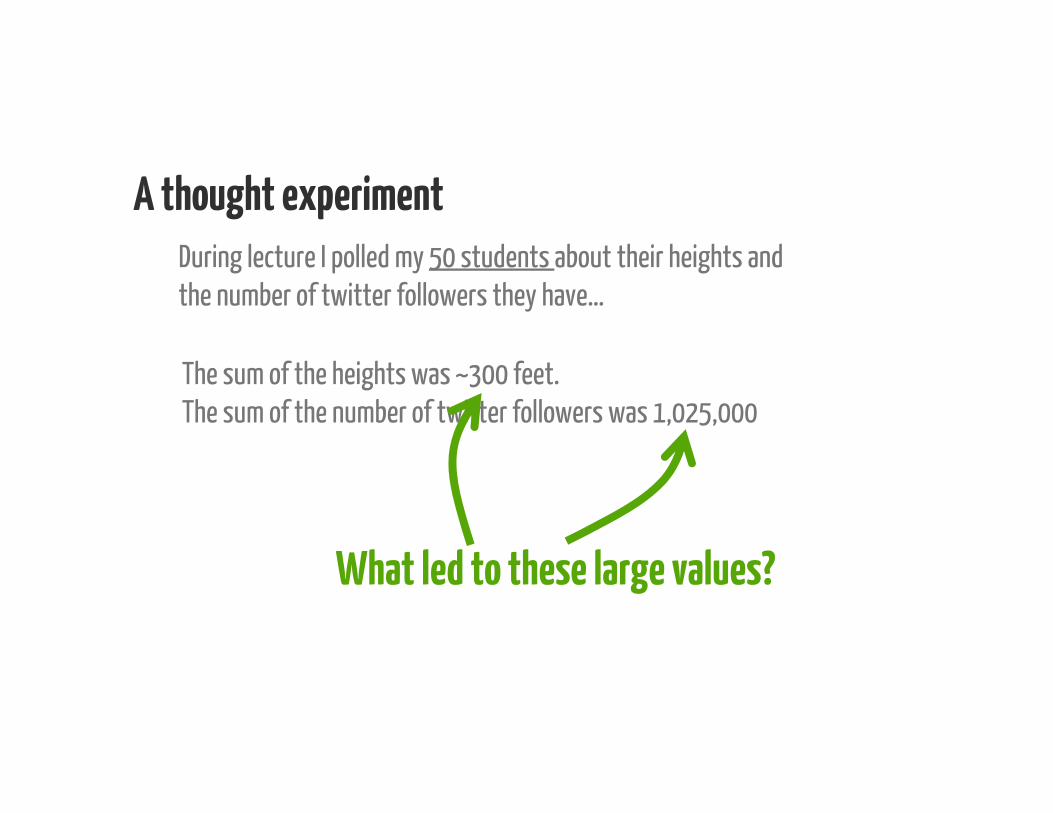
A thought experimentDuring lecture I polled my 50 students about their heights and the number of twitter followers they have…
The sum of the heights was ~300 feet.The sum of the number of twitter followers was 1,025,000
What led to these large values?
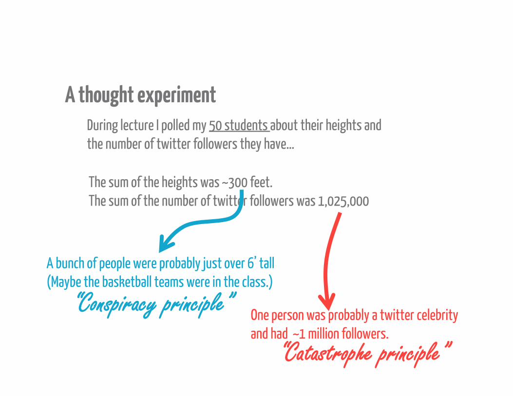
A thought experimentDuring lecture I polled my 50 students about their heights and the number of twitter followers they have…
The sum of the heights was ~300 feet.The sum of the number of twitter followers was 1,025,000
A bunch of people were probably just over 6’ tall(Maybe the basketball teams were in the class.)
One person was probably a twitter celebrity and had ~1 million followers.
“Catastrophe principle”
“Conspiracy principle”

ExampleConsider + i.i.d Weibull.Given + = , what is the marginal density of ?
Light-tailed Weibull
Heavy-tailed WeibullExponential
()
“Catastrophe principle”
“Conspiracy principle”
0

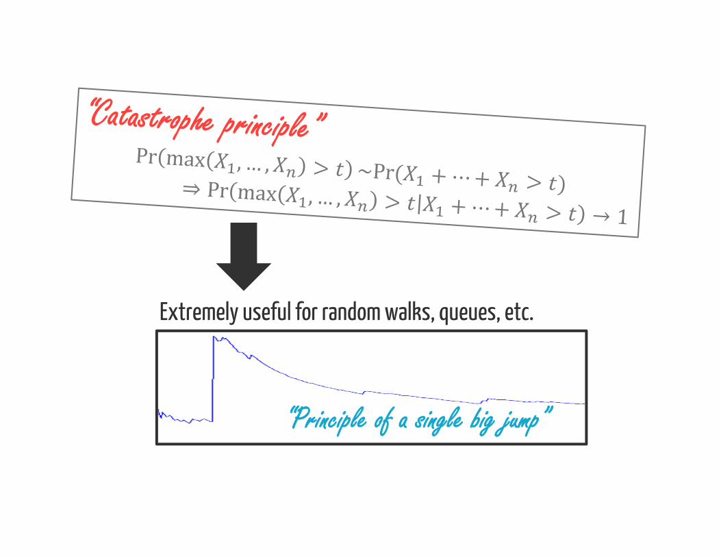
Extremely useful for random walks, queues, etc.
“Principle of a single big jump”
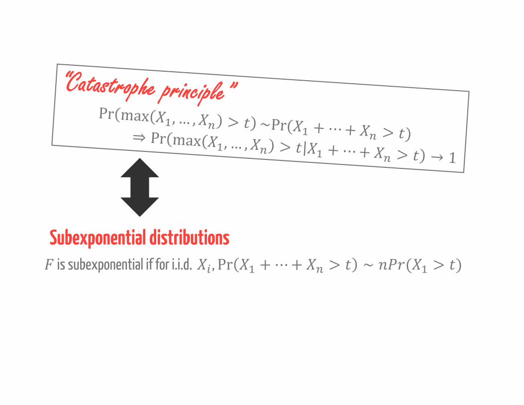
Subexponential distributionsis subexponential if for i.i.d. , Pr +⋯+ > ∼ ( > )

Subexponential distributionsis subexponential if for i.i.d. , Pr +⋯+ > ∼ ( > )
Pareto
Subexponential
Weibull
LogNormal
Regularly Varying
Heavy-tailed

Heavy-tailed distributions have many strange & beautiful properties
• The “Pareto principle”: 80% of the wealth owned by 20% of the population, etc.• Infinite variance or even infinite mean• Events that are much larger than the mean happen “frequently”….
These are driven by 3 “defining” properties1) Scale invariance2) The “catastrophe principle”3) The residual life ”blows up”

A thought experimentWhat happens to the expected remaining waiting time as we wait
…for a table at a restaurant?…for a bus?…for the response to an email?
residual life
If you don’t get it quickly, you never will…
The remaining wait drops as you wait
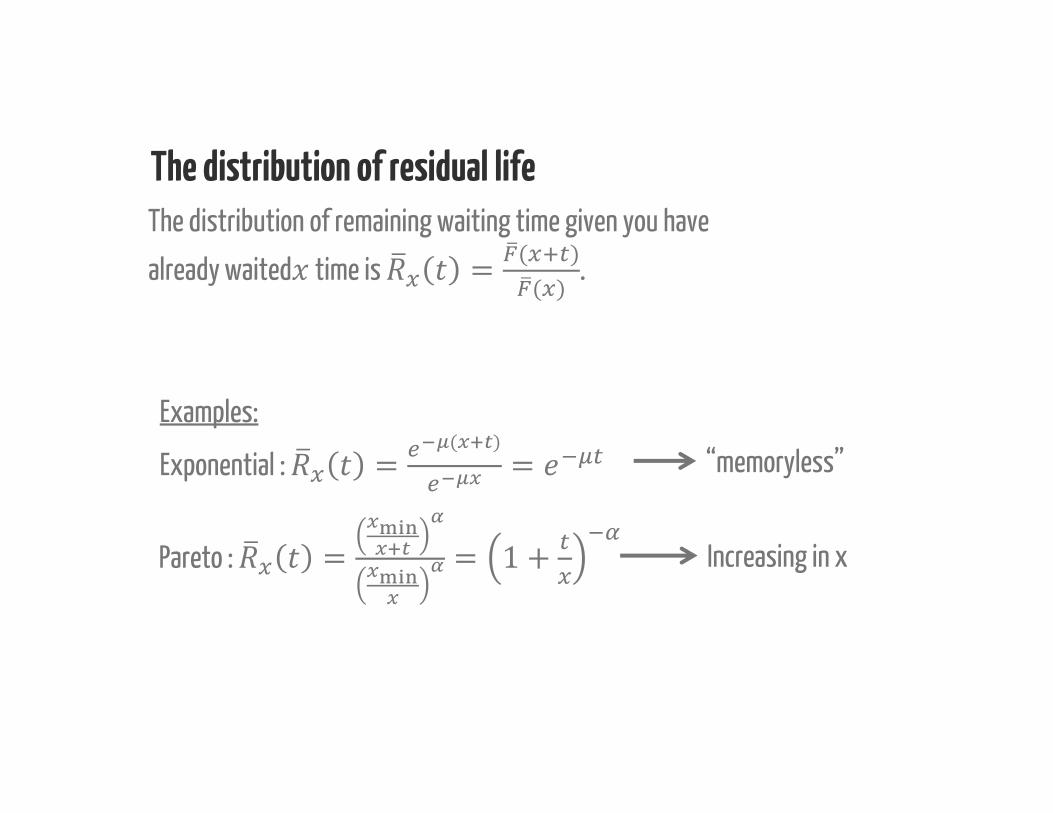
The distribution of residual lifeThe distribution of remaining waiting time given you have
already waited time is = ( )( ) .
Examples:
Exponential : = ( ) = “memoryless”
Pareto : = = 1 + Increasing in x

The distribution of residual lifeThe distribution of remaining waiting time given you have
already waited time is = ( )( ) .
Mean residual life
Hazard rate
= − > = ∫= = (0)
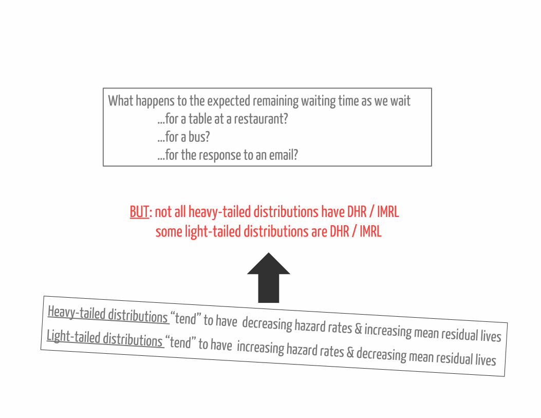
BUT: not all heavy-tailed distributions have DHR / IMRLsome light-tailed distributions are DHR / IMRL
What happens to the expected remaining waiting time as we wait…for a table at a restaurant?…for a bus?…for the response to an email?

BUT: not all heavy-tailed distributions have DHR / IMRLsome light-tailed distributions are DHR / IMRL
Long-tailed distributionsis long-tailed if lim→ = lim→ ( )( ) = 1 for all

Long-tailed distributions
Pareto
Subexponential
Weibull
LogNormal
Regularly Varying
Heavy-tailed
Long-tailed distributions
is long-tailed if lim→ = lim→ ( )( ) = 1 for all

Pareto
Subexponential
Weibull
LogNormal
Regularly Varying
Heavy-tailed
Long-tailed distributions
Difficult to work with in general
Pareto
Subexponential
Weibull
LogNormal
Regularly Varying
Heavy-tailed
Long-tailed distributions
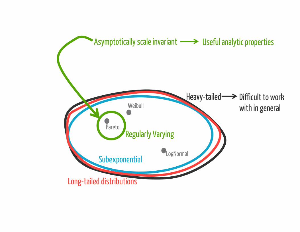
Asymptotically scale invariant Useful analytic properties
Difficult to work with in general

Pareto
Subexponential
Weibull
LogNormal
Regularly Varying
Heavy-tailed
Long-tailed distributions
Catastrophe principle Useful for studying random walks
Difficult to work with in general
Pareto
Subexponential
Weibull
LogNormal
Regularly Varying
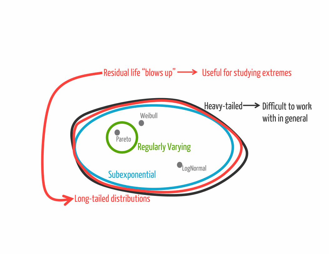
Heavy-tailed
Long-tailed distributions
Residual life “blows up” Useful for studying extremes
Difficult to work with in general

Heavy-tailed phenomena are treated as something
Mysterious, Surprising, & Controversial
1. Properties 2. Emergence
3. Identification
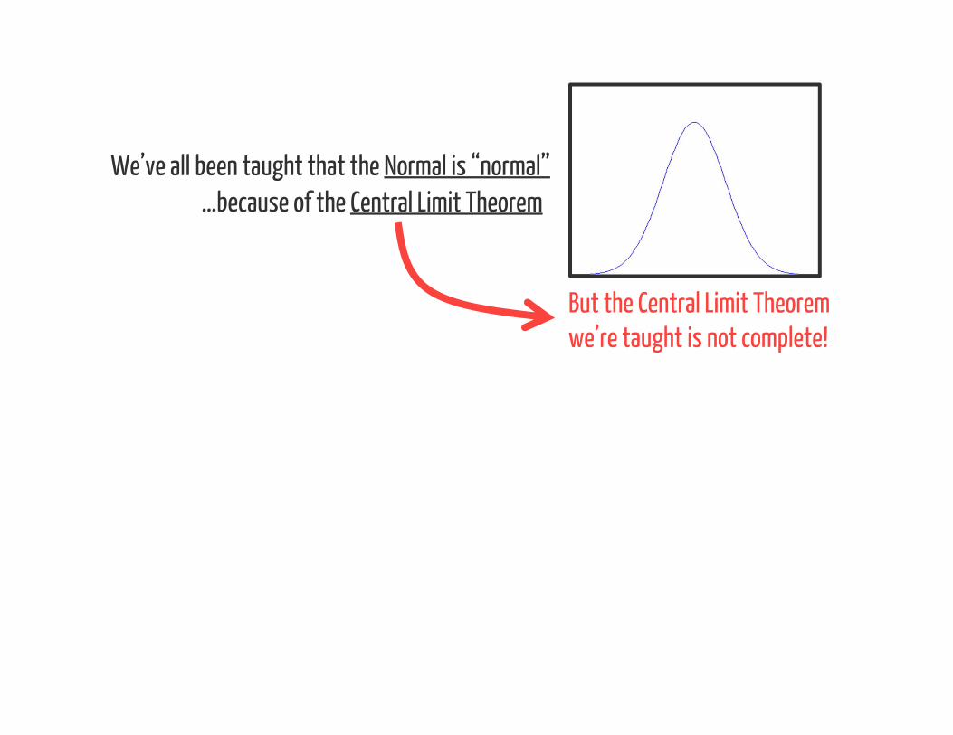
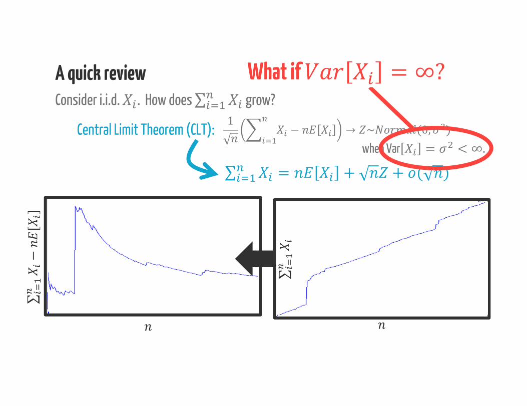
We’ve all been taught that the Normal is “normal”…because of the Central Limit Theorem
But the Central Limit Theorem we’re taught is not complete!
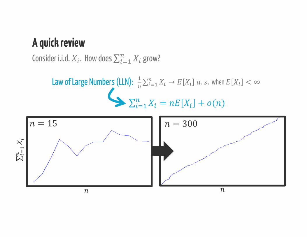
Law of Large Numbers (LLN): ∑ → . . when < ∞∑ = + ( )A quick reviewConsider i.i.d. . How does ∑ grow?
= 15 = 300
∑
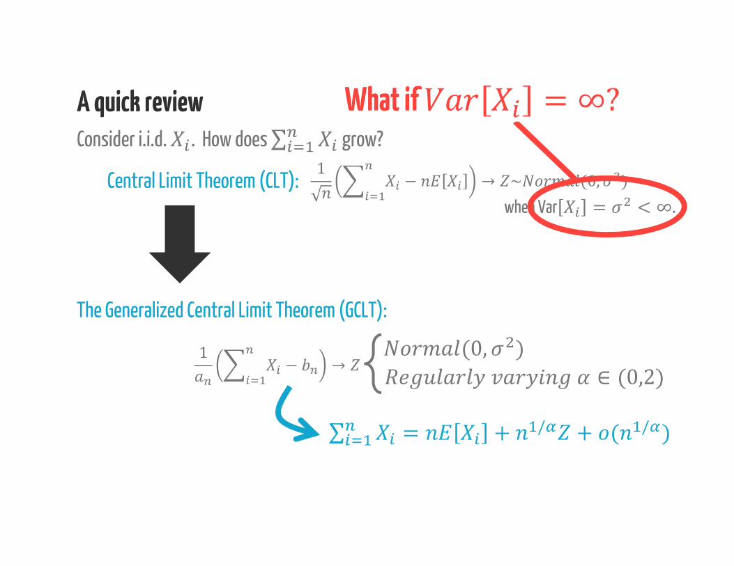
A quick reviewConsider i.i.d. . How does ∑ grow?
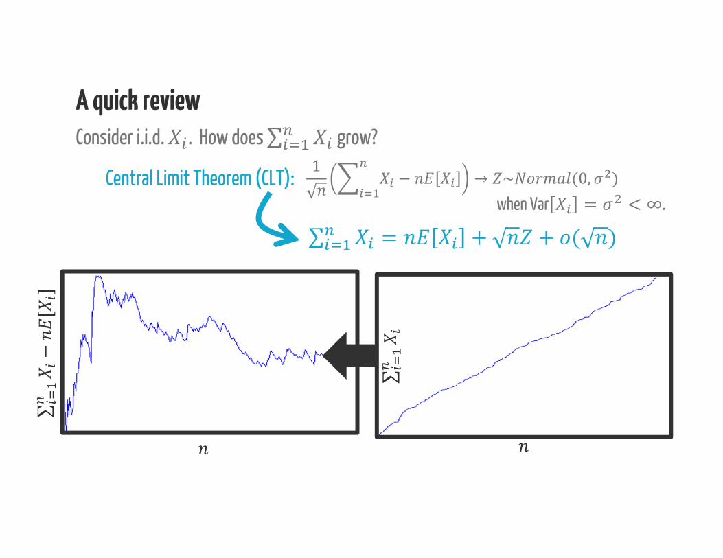
Central Limit Theorem (CLT):when Var = < ∞.1 − → ~ (0, )∑ = + + ( )
∑∑−[
]

A quick reviewConsider i.i.d. . How does ∑ grow?
Central Limit Theorem (CLT):when Var = < ∞.1 − → ~ (0, )∑ = + + ( )
Two key assumptions
∑∑−[
]
A quick reviewConsider i.i.d. . How does ∑ grow?
Central Limit Theorem (CLT):when Var = < ∞.1 − → ~ (0, )∑ = + + ( )
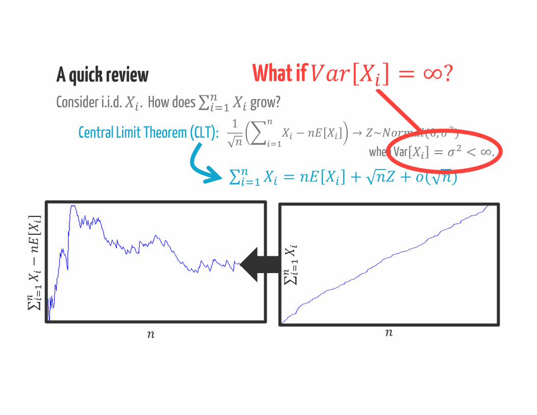
What if
∑∑−[
]
A quick reviewConsider i.i.d. . How does ∑ grow?
Central Limit Theorem (CLT):when Var = < ∞.1 − → ~ (0, )∑ = + + ( )= 300
What if
∑−[
]
∑
A quick reviewConsider i.i.d. . How does ∑ grow?
Central Limit Theorem (CLT):when Var = < ∞.1 − → ~ (0, )
What if
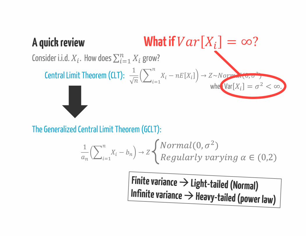
The Generalized Central Limit Theorem (GCLT):1 − → (0, ) ∈ (0,2)∑ = + / + ( / )
A quick reviewConsider i.i.d. . How does ∑ grow?
Central Limit Theorem (CLT):when Var = < ∞.1 − → ~ (0, )
What if
The Generalized Central Limit Theorem (GCLT):1 − → (0, ) ∈ (0,2)
Consider i.i.d. . How does ∑ grow?
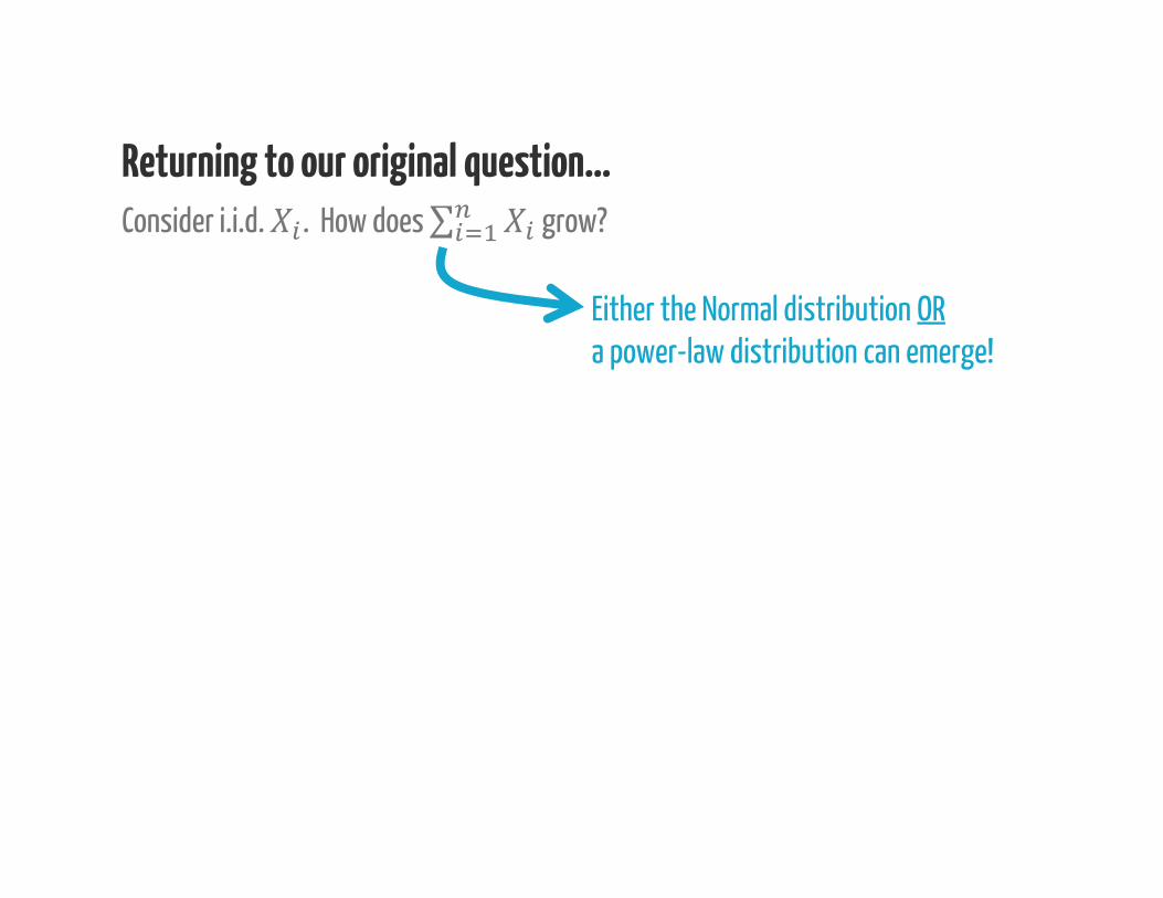
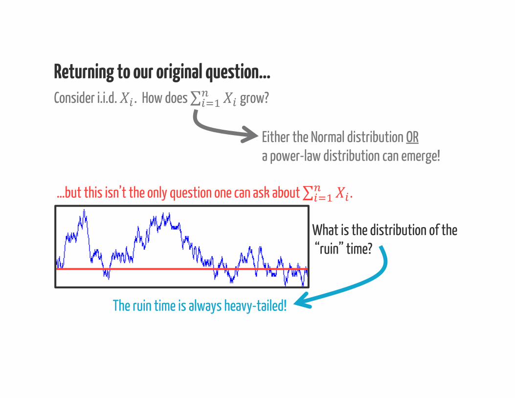
Returning to our original question…
Either the Normal distribution ORa power-law distribution can emerge!
Consider i.i.d. . How does ∑ grow?
Returning to our original question…
Either the Normal distribution ORa power-law distribution can emerge!
…but this isn’t the only question one can ask about ∑ .
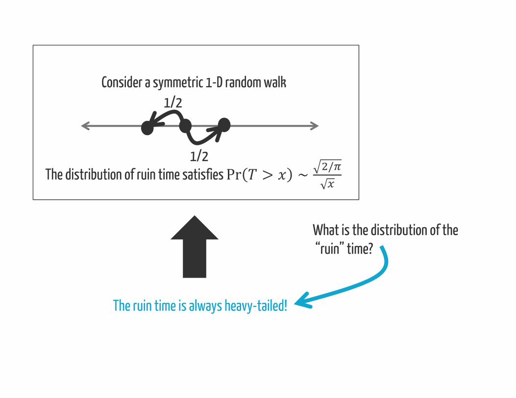
What is the distribution of the“ruin” time?
The ruin time is always heavy-tailed!
What is the distribution of the“ruin” time?
The ruin time is always heavy-tailed!
Consider a symmetric 1-D random walk
1/2
1/2
The distribution of ruin time satisfies Pr > ∼ /

We’ve all been taught that the Normal is “normal”…because of the Central Limit Theorem
Heavy-tails are more “normal” than the Normal!1. Additive Processes2. Multiplicative Processes3. Extremal Processes

A simple multiplicative process= ⋅ ⋅ … ⋅ ,where are i.i.d. and positive
Ex: incomes, populations, fragmentation, twitter popularity…
“Rich get richer”

Multiplicative processes almost always lead to heavy tails
An example:, ∼ ( )Pr ⋅ > ≥ Pr >=⇒ ⋅ is heavy-tailed!
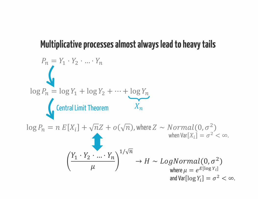
= ⋅ ⋅ … ⋅Multiplicative processes almost always lead to heavy tails
log = log + log +⋯+ logCentral Limit Theoremlog = + + ,where ∼ (0, )
when Var = < ∞.⋅ ⋅ … ⋅ / → ∼ (0, )where = [ ]and Var log = < ∞.
⋅ ⋅ … ⋅ / → ∼ (0, )where = [ ]and Var log = < ∞.
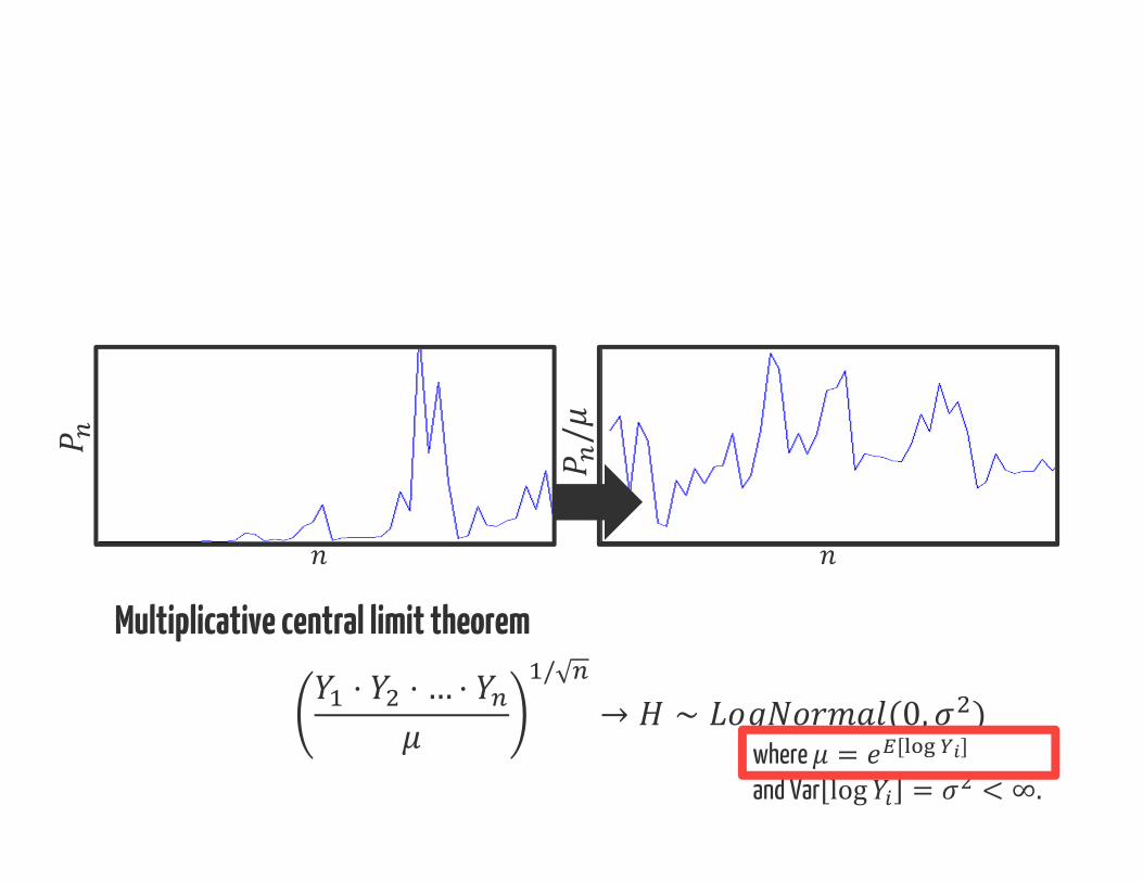
Multiplicative central limit theorem /
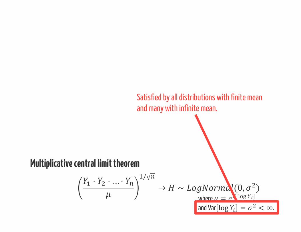
⋅ ⋅ … ⋅ / → ∼ (0, )where = [ ]and Var log = < ∞.
Satisfied by all distributions with finite mean and many with infinite mean.
Multiplicative central limit theorem

“Rich get richer”
LogNormals emergeHeavy-tails
A simple multiplicative process
Ex: incomes, populations, fragmentation, twitter popularity…
= ⋅ ⋅ … ⋅ ,where are i.i.d. and positive

A simple multiplicative process
Ex: incomes, populations, fragmentation, twitter popularity…
Multiplicative process with a lower barrier
Multiplicative process with noise= += min( , ) Distributions that are
approximately power-law emerge
= ⋅ ⋅ … ⋅ ,where are i.i.d. and positive
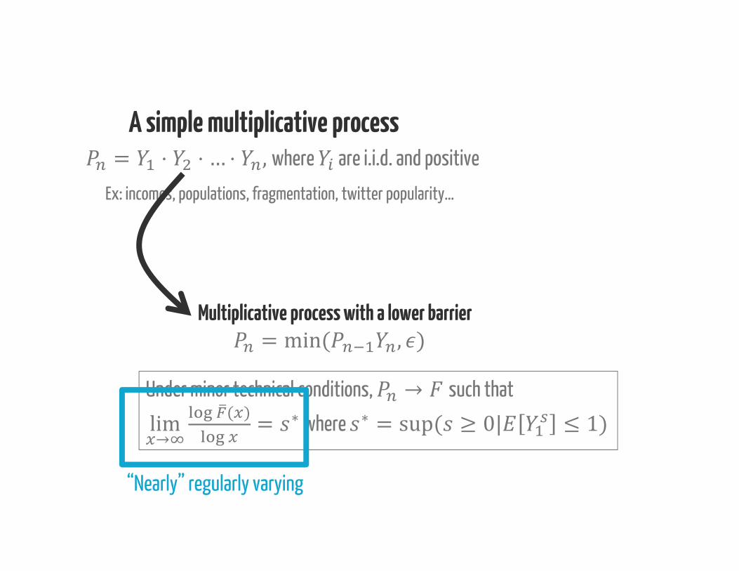
A simple multiplicative process
Ex: incomes, populations, fragmentation, twitter popularity…
Multiplicative process with a lower barrier= min( , )
= ⋅ ⋅ … ⋅ ,where are i.i.d. and positive
Under minor technical conditions, → such thatlim→ ( ) = ∗ where ∗ = sup( ≥ 0| ≤ 1)“Nearly” regularly varying

We’ve all been taught that the Normal is “normal”…because of the Central Limit Theorem
Heavy-tails are more “normal” than the Normal!1. Additive Processes2. Multiplicative Processes3. Extremal Processes
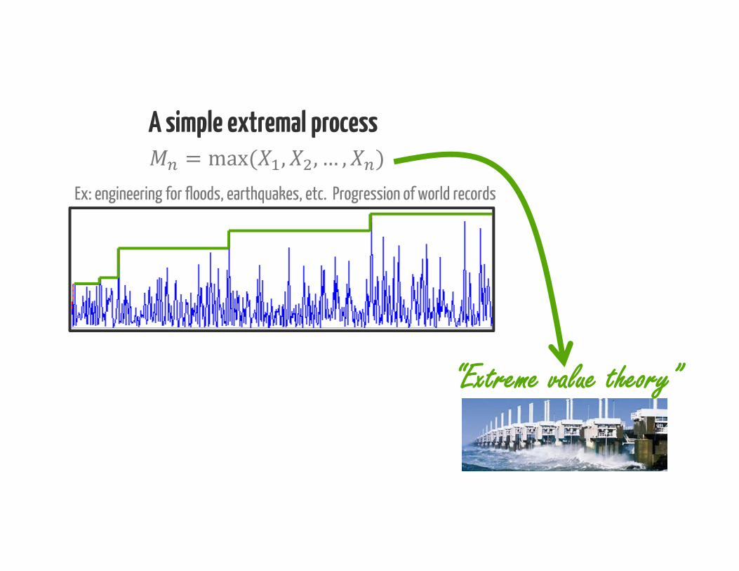
A simple extremal process= max( , , … , )Ex: engineering for floods, earthquakes, etc. Progression of world records
“Extreme value theory”
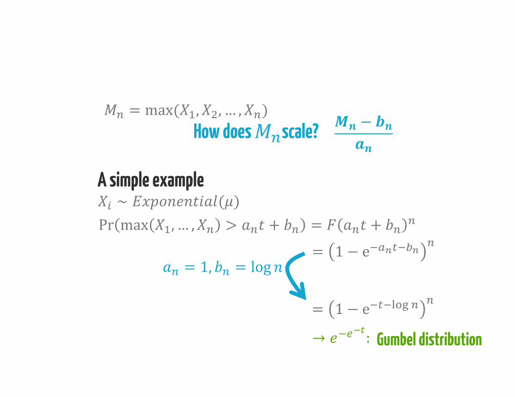
A simple example∼ ( )Pr max ,… , > + = +How does scale?
= 1 − e
= max( , , … , ) −
→ := 1 − e= 1, = logGumbel distribution
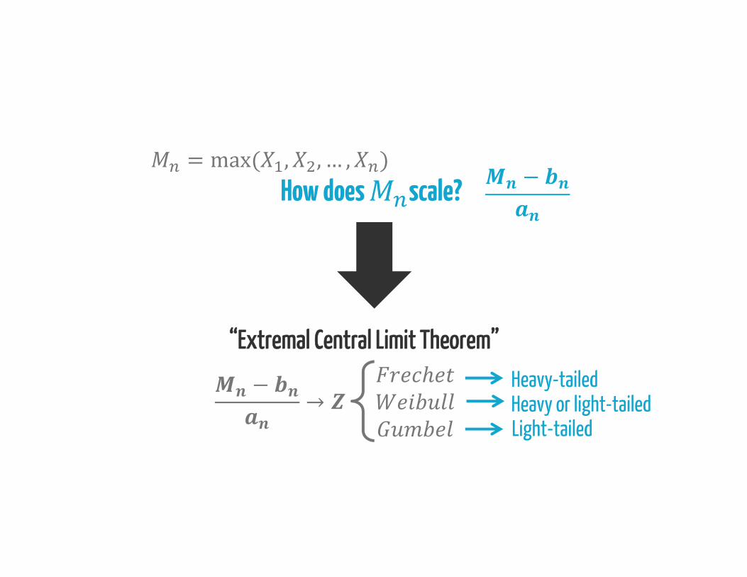
How does scale? = max( , , … , ) −
“Extremal Central Limit Theorem”− → Heavy-tailedHeavy or light-tailedLight-tailed
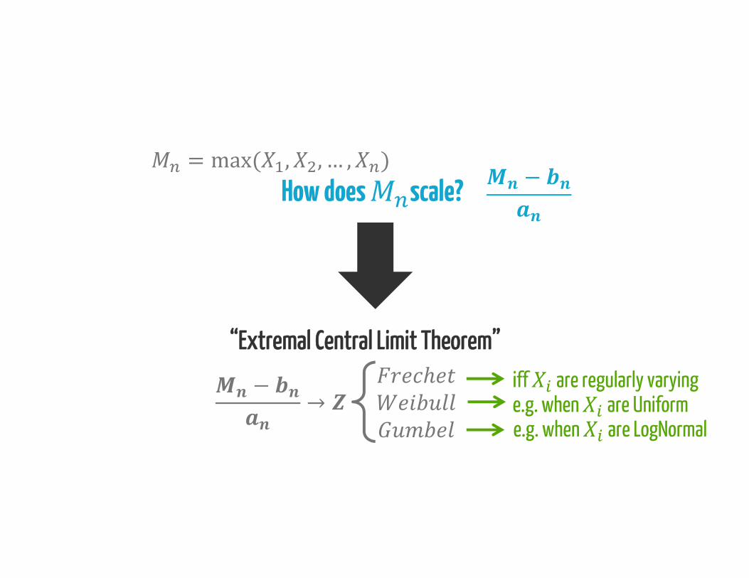
How does scale? = max( , , … , ) −
“Extremal Central Limit Theorem”iff are regularly varyinge.g. when are Uniforme.g. when are LogNormal
− →
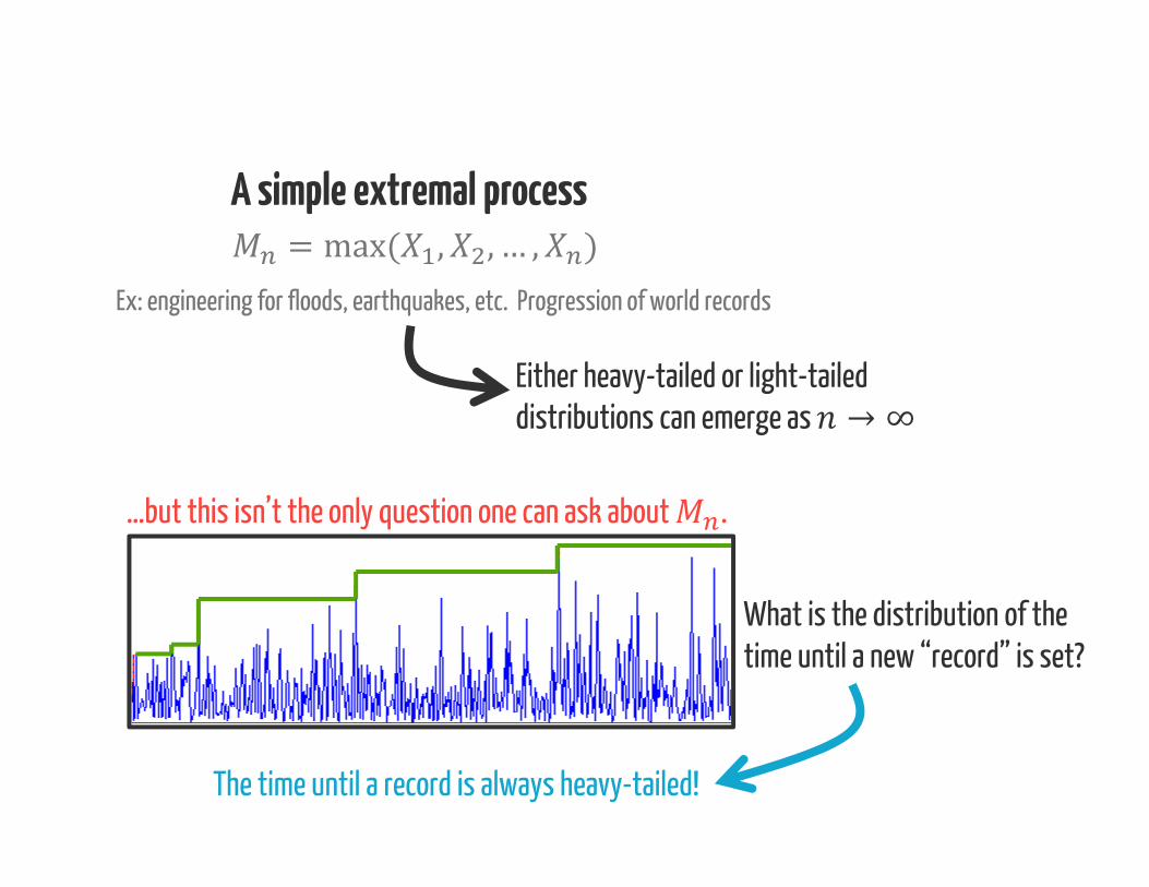
A simple extremal process= max( , , … , )Ex: engineering for floods, earthquakes, etc. Progression of world records
Either heavy-tailed or light-tailed distributions can emerge as → ∞
…but this isn’t the only question one can ask about .
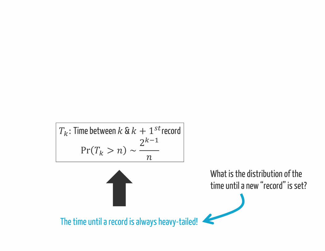
What is the distribution of thetime until a new “record” is set?
The time until a record is always heavy-tailed!
The time until a record is always heavy-tailed!
:Time between & + 1 recordPr > ∼ 2What is the distribution of thetime until a new “record” is set?

We’ve all been taught that the Normal is “normal”…because of the Central Limit Theorem
Heavy-tails are more “normal” than the Normal!1. Additive Processes2. Multiplicative Processes3. Extremal Processes

Heavy-tailed phenomena are treated as something
Mysterious, Surprising, & Controversial
1. Properties 2. Emergence
3. Identification
Heavy-tailed phenomena are treated as something
Mysterious, Surprising, & Controversial
1999 Sigcomm paper – 4500+ citations!
BUT…
2005, ToN
Similar stories in electricity nets, citation nets, …

A “typical” approach for identifying of heavy tails: Linear Regression
Heavy-tailedor light-tailed?
value
frequ
ency
“frequency plot”
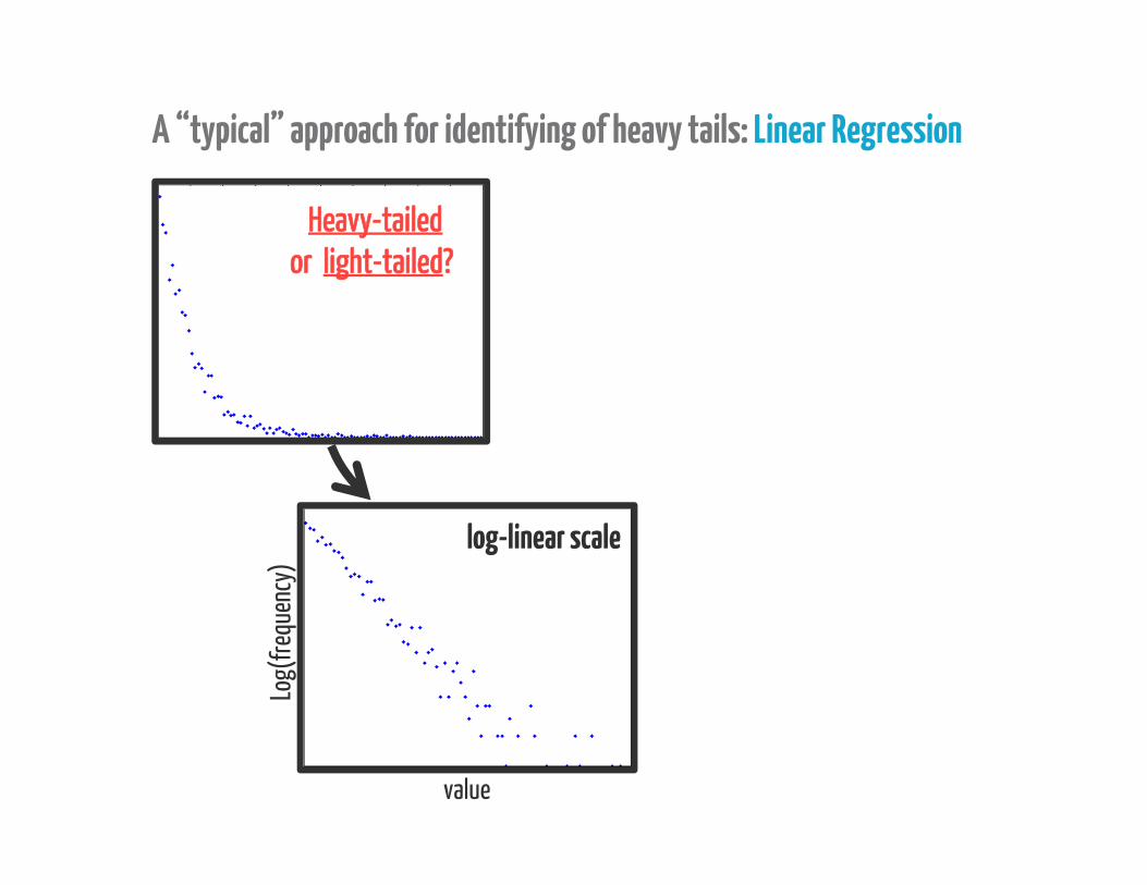
A “typical” approach for identifying of heavy tails: Linear Regression
Heavy-tailedor light-tailed?
log-linear scale
Log(
frequ
ency
)
value
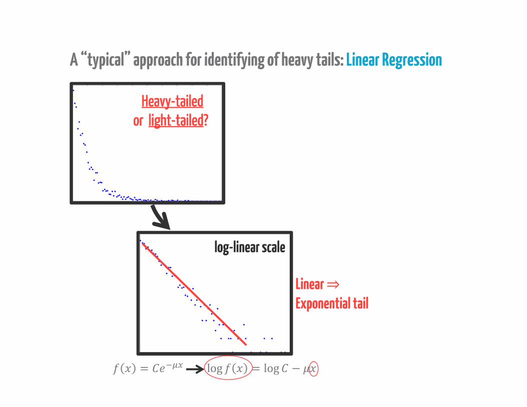
A “typical” approach for identifying of heavy tails: Linear Regression
Heavy-tailedor light-tailed?
= log = log −Linear ⇒Exponential tail
log-linear scale
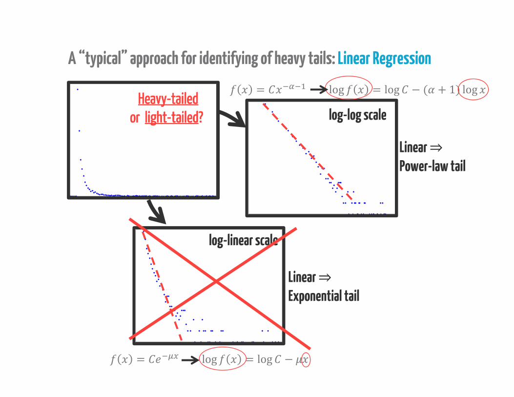
A “typical” approach for identifying of heavy tails: Linear Regression
Heavy-tailedor light-tailed? log-log scale
= log = log −Linear ⇒Exponential tail
log-linear scale
= log = log − ( + 1) logLinear ⇒Power-law tail
log-linear scale
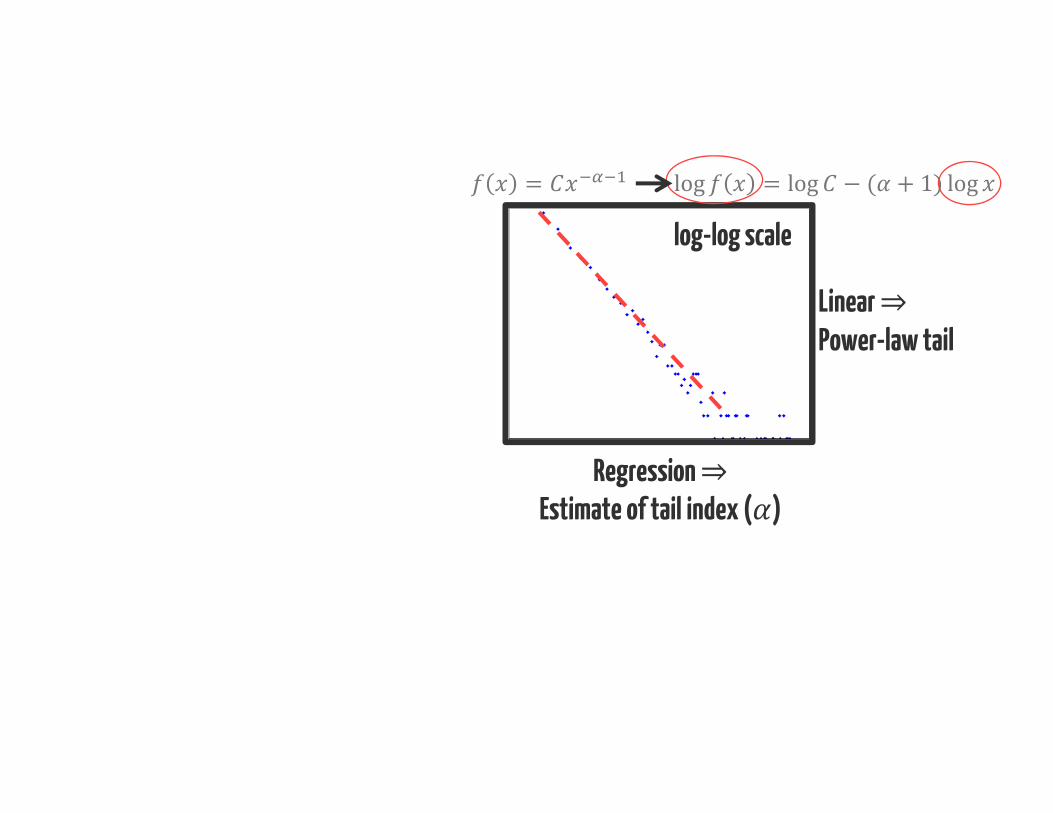
log-log scale
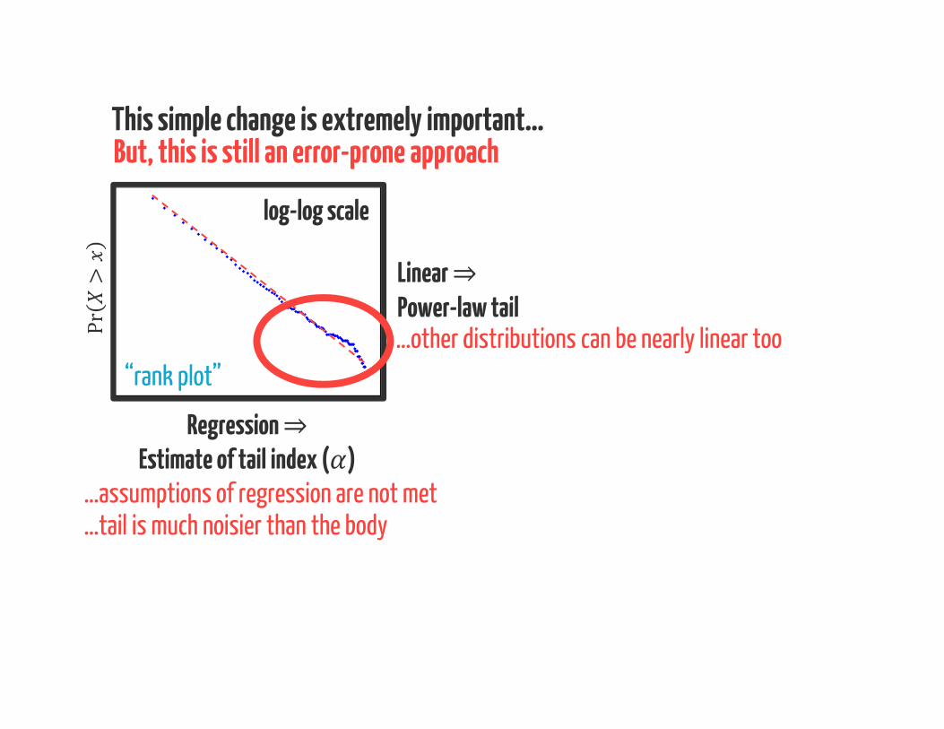
Regression ⇒Estimate of tail index ( )
= log = log − ( + 1) logLinear ⇒Power-law tail
log-log scale
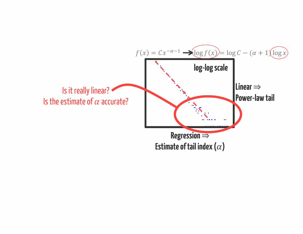
= log = log − ( + 1) logLinear ⇒Power-law tail
Regression ⇒Estimate of tail index ( )
Is it really linear?Is the estimate of accurate?
log-log scale
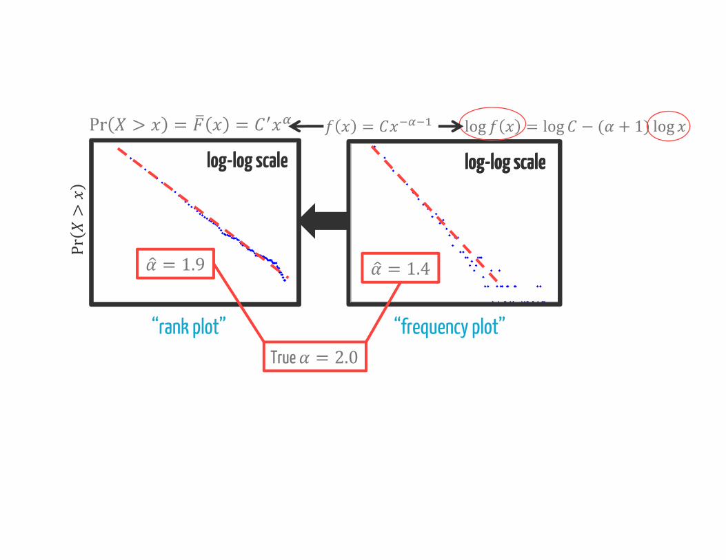
Pr>log-log scale log-log scalelog-log scale
Pr > = =
“rank plot”
= log = log − ( + 1) log
“frequency plot”
= 1.4= 1.9True = 2.0

This simple change is extremely important…
log-log scalelog-log scale log-log scalelog-log scale
“rank plot” “frequency plot”
Pr>
log-log scale
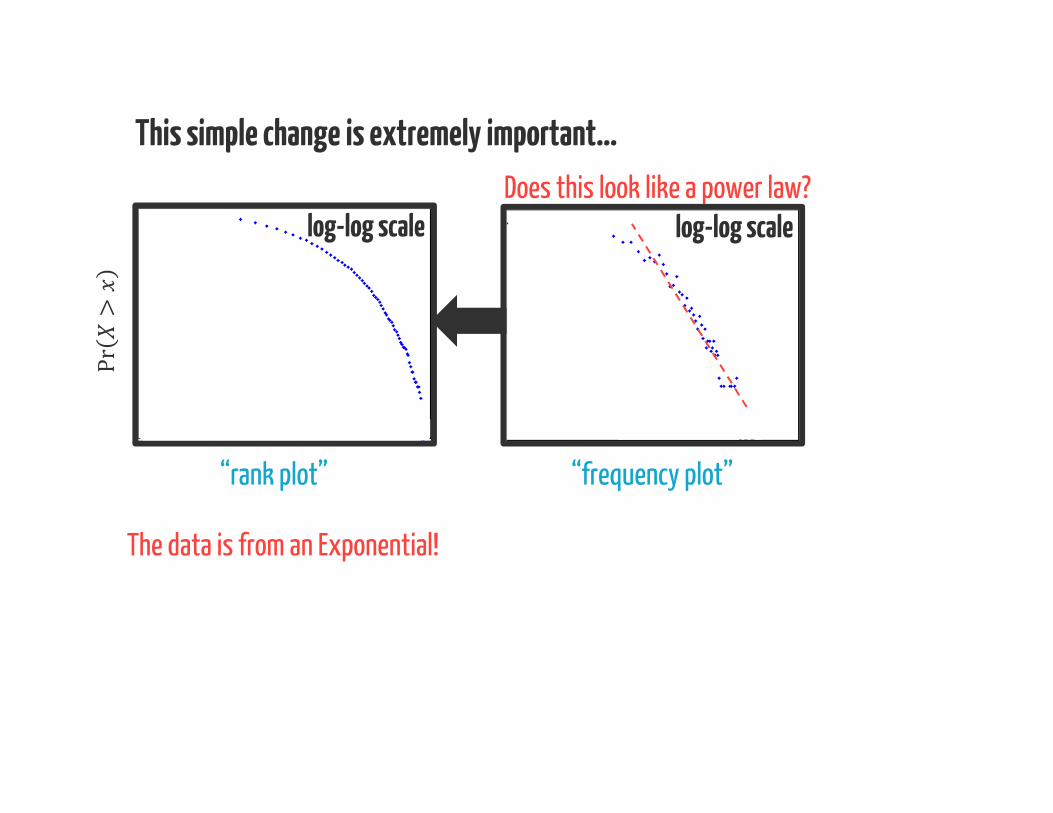
This simple change is extremely important…
“frequency plot”
The data is from an Exponential!
Does this look like a power law?log-log scale
“rank plot”
Pr>

log-log scale
“frequency plot”
Electricity grid degree distribution
= 3(from Science)
This mistake has happened A LOT!
“rank plot”
log-linear scale
Pr>

This mistake has happened A LOT!
log-log scale
“frequency plot”
WWW degree distribution
= 1.1(from Science)
“rank plot”
log-log scale
= 1.7Pr>

Linear ⇒Power-law tail
Regression ⇒Estimate of tail index ( )
But, this is still an error-prone approach
…other distributions can be nearly linear too
This simple change is extremely important…
log-log scale
Pr>log-log scale
“rank plot” …log-log scale log-log scale
WeibullLognormal
log-log scale
Pr>log-log scale
Regression ⇒Estimate of tail index ( )
…assumptions of regression are not met
But, this is still an error-prone approachThis simple change is extremely important…
…tail is much noisier than the body
Linear ⇒Power-law tail…other distributions can be nearly linear too
“rank plot”
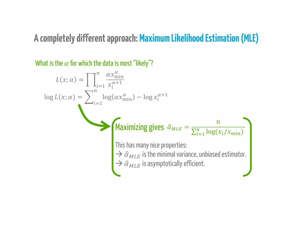
A completely different approach: Maximum Likelihood Estimation (MLE)
What is the for which the data is most “likely”?; =log ( ; ) = log − log= ∑ log( / )Maximizing gives
This has many nice properties: is the minimal variance, unbiased estimator. is asymptotically efficient.
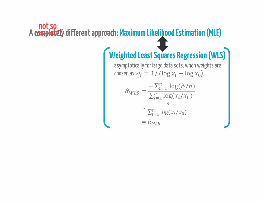
A completely different approach: Maximum Likelihood Estimation (MLE)not so
= −∑ log( ̂ / )∑ log( / )asymptotically for large data sets, when weights are chosen as = 1/ (log − log ).
∼ ∑ log( / )=
Weighted Least Squares Regression (WLS)
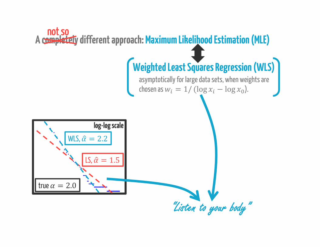
A completely different approach: Maximum Likelihood Estimation (MLE)not so
Weighted Least Squares Regression (WLS)
log-log scale
“Listen to your body”
asymptotically for large data sets, when weights are chosen as = 1/ (log − log ).
WLS, = 2.2LS, = 1.5
“rank plot”true = 2.0

A quick summary of where we are:
Suppose data comes from a power-law (Pareto) distribution = .
Then, we can identify this visually with a log-log plot, and we can estimate using either MLE or WLS.

log-log scale
“rank plot”
Suppose data comes from a power-law (Pareto) distribution = .
Then, we can identify this visually with a log-log plot, and we can estimate using either MLE or WLS.
What if the data is not exactly a power-law? What if only the tail is power-law?
But, where does the tail start?
Can we just use MLE/WLS on the “tail”?
Impossible to answer…

An exampleSuppose we have a mixture of power laws:
…but, suppose we use as our cutoff: 1 → ( ) + (1 − )( ) ≠
Suppose we have a mixture of power laws:= + 1 − <We want → as → ∞.

Identifying power-law distributions“Listen to your body”
Identifying power-law tails“Let the tail do the talking”
MLE/WLS
v.s.
Extreme value theory

Returning to our exampleSuppose we have a mixture of power laws:= + 1 − <We want → as → ∞.…but, suppose we use as our cutoff: 1 → ( ) + (1 − )( )
The bias disappears as → ∞ !
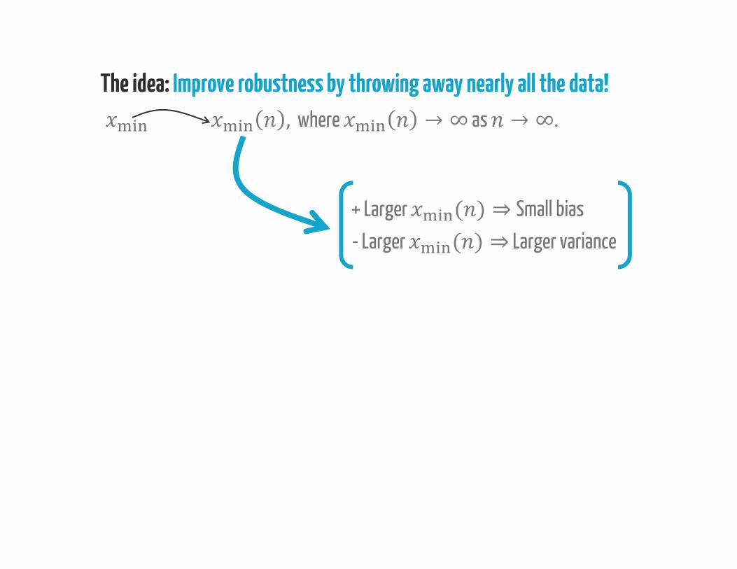
The idea: Improve robustness by throwing away nearly all the data!, where → ∞ as → ∞.
+ Larger ( ) ⇒Small bias- Larger ( ) ⇒ Larger variance

, where → ∞ as → ∞.
The Hill Estimator, = ∑ logwhere ( )is the th largest data point
Looks almost like the MLE, butuses order th order statistic
The idea: Improve robustness by throwing away nearly all the data!

The Hill Estimator
where ( )is the th largest data point …how do we choose ?
, → as → ∞ if / →0 & → ∞throw away nearly all the data,
but keep enough data for consistency
The idea: Improve robustness by throwing away nearly all the data!, where → ∞ as → ∞.
, = ∑ log Looks almost like the MLE, butuses order th order statistic

The Hill Estimator
where ( )is the th largest data point …how do we choose ?
, → as → ∞ if / →0 & → ∞Throw away everything except the outliers!
The idea: Improve robustness by throwing away nearly all the data!, where → ∞ as → ∞.
, = ∑ log Looks almost like the MLE, butuses order th order statistic

Choosing in practice: The Hill plot
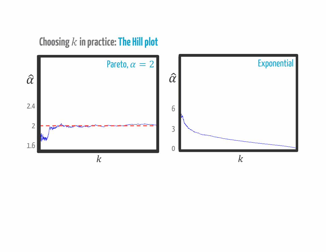
Choosing in practice: The Hill plot
2.4
2
1.6
Pareto, = 26
3
0
Exponential

Choosing in practice: The Hill plot
2.4
2
1.6
Pareto, = 22.5
2
1.5
1
Mixture, with Pareto-tail, = 2
log-log scale
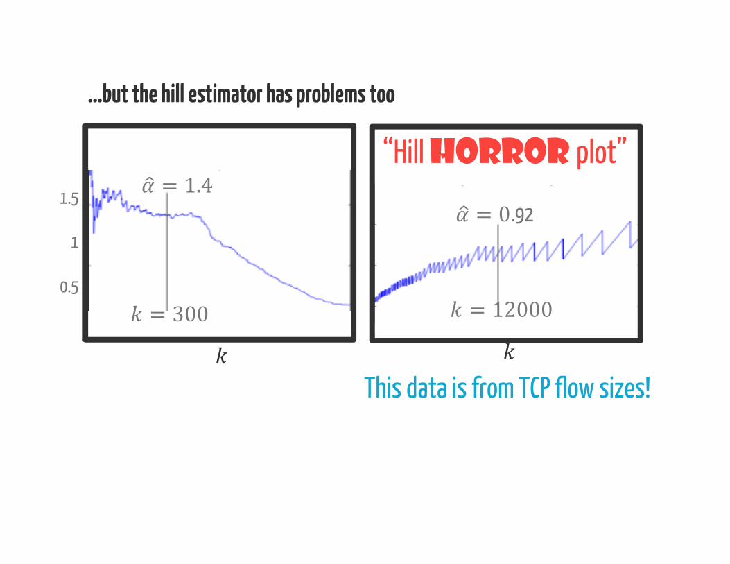
…but the hill estimator has problems too
1.5
1
0.5 = 300= 1.4
This data is from TCP flow sizes!
= 12000= 0.92
“Hill horror plot”

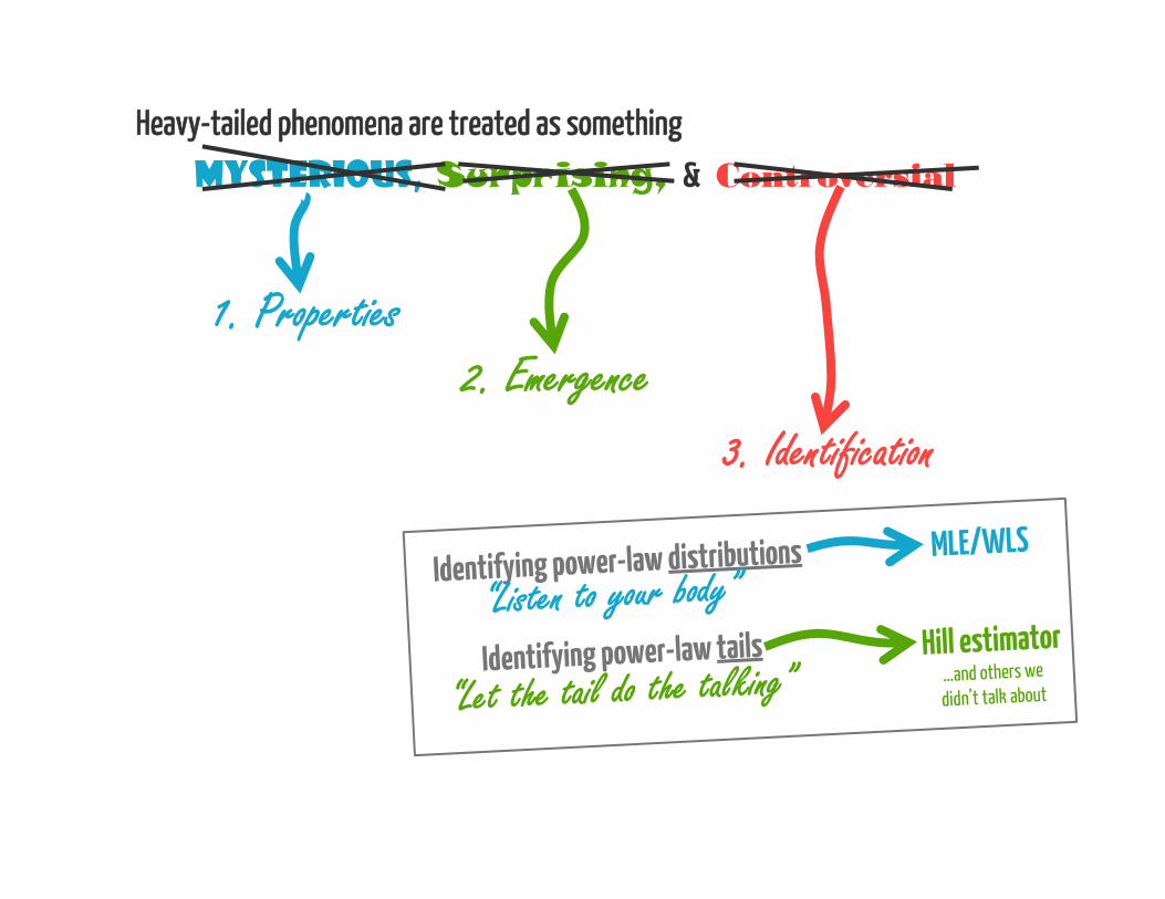
Identifying power-law distributions“Listen to your body”
Identifying power-law tails“Let the tail do the talking”
MLE/WLS
Hill estimator
It’s dangerous to rely on any one technique!(see our forthcoming book for other approaches)

Heavy-tailed phenomena are treated as something
Mysterious, Surprising, & Controversial
1. Properties 2. Emergence
3. Identification

Heavy-tailed phenomena are treated as something
Mysterious, Surprising, & Controversial
1. Properties 2. Emergence
3. Identification Pareto
Subexponential
Weibull
LogNormal
Regularly Varying
Heavy-tailed
Long-tailed distributions

Heavy-tailed phenomena are treated as something
Mysterious, Surprising, & Controversial
1. Properties 2. Emergence
3. Identification
Heavy-tailed phenomena are treated as something
Mysterious, Surprising, & Controversial
1. Properties 2. Emergence
3. Identification

The Fundamentals of Heavy TailsProperties, Emergence, & Identification
Jayakrishnan Nair, Adam Wierman, Bert Zwart


![Extremal shot noises, heavy tails and max-stable random fieldscdombry.perso.math.cnrs.fr/[D14].pdf · 2014-01-08 · Extremal shot noises, heavy tails and max-stable random fields](https://img.pdfslide.us/doc/110x75/5e9539bfdce8084e3c72d0ce/extremal-shot-noises-heavy-tails-and-max-stable-random-d14pdf-2014-01-08.jpg)