Models with Long Range Dependence and Heavy Tailsrobotics.eecs.berkeley.edu/~wlr/ADCN-slides/review1010/Anantharam.pdfModels with Long Range Dependence and Heavy Tails Vivek S. Borkar1

Models with Long Range Dependence and Heavy Tails

Vivek S. Borkar1 Venkat Anantharam2 Barlas Oguz3

1School of Technology and Computer Science,Tata Institute of Fundamental Research,

Homi Bhabha Road, Mumbai 400005, India.

2,3Department of Electrical Engineering and Computer SciencesUniversity of California, Berkeley

Berkeley, California

October 14, 2010

Outline

Stochastic Approximation with ’bad’ noise

LRD Markov Chain theorem with examples

(Berkeley) LRD Models Oct 2010 2 / 69

Stochastic Approximation with ’bad’ Noise

Venkat Anantharam, Vivek Borkar

Stochastic Approximation

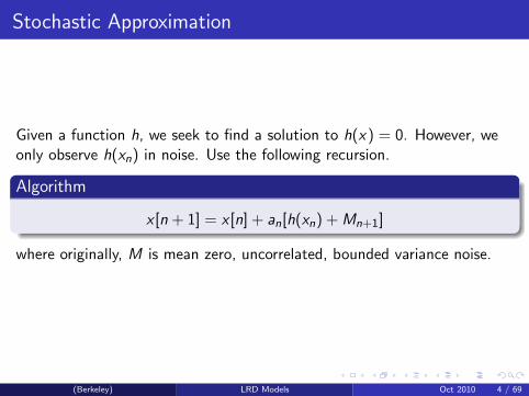
Given a function h, we seek to find a solution to h(x ) = 0. However, weonly observe h(xn) in noise. Use the following recursion.

Algorithm

x [n + 1] = x [n] + an[h(xn) + Mn+1]

where originally, M is mean zero, uncorrelated, bounded variance noise.


Stochastic Approximation

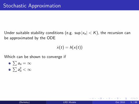
Under suitable stability conditions (e.g. sup |xn| < K ), the recursion canbe approximated by the ODE

x(t) = h(x(t))

Which can be shown to converge if∑an =∞∑a2n <∞


ROBBINS-MONRO SCHEME (1951)

to solve h(x) = 0 given noisy measurements of h(·) : Rd → Rd :

xn+1 = xn + a(n)[h(xn) + Mn+1], n ≥ 0.

||h(x)− h(y)|| ≤ L||x − y || ∀x , yE [Mn+1|xi ,Mi , i ≤ n] = 0 ∀n. (’martingale difference’)

E [||Mn+1||2|xi ,Mi , i ≤ n] ≤ K (1 + ||xn||2) ∀n.a(n) > 0,

∑n a(n) =∞,

∑n a(n)2 <∞.


The o.d.e. approach:

(Derevitskii - Fradkov - Ljung)Consider the iteration as a noisy discretization of the o.d.e. (ordinarydifferential equation)

x(t) = h(x(t))

with step-sizes {a(n)}. If

xns track x(t) in a suitable sense, and

x(t)→ H := {x : h(x) = 0},then we can expect xn → H a.s.


Example 1. Gradient schemes

Here h(x) = −5 F (x). As an example, consider N users share an ergodicMarkov channel with stationary distribution ν.Aim: Minimize average power subject to a minimum rate constraint.

A = {unit coordinate vectors in RN} (i-th vector ≈ choice of i-thuser for the slot).

p2(y |x) = conditional distribution of the user given channel state,

p1(q|y , x) = conditional distribution of this users power consumption.


Problem:

min

∫ν(dx)

∑y∈A

∫ ∞0

p1(dq|y , x)p2(y |x)q

subject to ∫ν(dx)

∑y∈A

∫ ∞0

p1(dq|y , x) log(1 + qyixi ) ≥ Ci ∀i .

Central idea: Use the Lagrange multiplier formulation in order to cast theconstrained optimization problem as an unconstrained min-max (=max-min) problem, do the minimization over both the users and powerexplicitly as above, and the maximization over Lagrange multipliers bystochastic approximation. The foregoing theory ensures desiredasymptotics (also veried by simulation experiments).


Solution

The optimal solution is to select user

k = arg mini

((λi −

1

xi)+ − λi [log(1 + (λi −

1

xi)+xi )− Ci ]

),

who will transmit power

q∗ = (λk −1

xk)+,

λi being the Lagrange multiplier associated with the i-th constraint.{λi} can be learnt adaptively by the stochastic gradient scheme

λi (n + 1) = Γ(λi (n)− a(n)yi (n)[log(1 + (λi −1

xi)+xi (n))− Ci ]), ∀i .

Here yi (n) = I{αi ≤ αj , j 6= i} for

αi = q∗i − λi (n)[log(1 + (λi −1

xi (n))+xi (n))− Ci ], 1 ≤ i ≤ N,

and Γ is projection to [0, L] for a large L.(Berkeley) LRD Models Oct 2010 10 / 69

Example 2. Fixed point iterations

Here, h(x) = F (x)− x , F a contraction w.r.t. a suitable norm.

Aim: Find its unique fixed point x given by x = F (x ). (≈ globallyasymptotically stable equilibrium for the o.d.e. x(t) = F (x(t))− x(t).This can be extended to nonexpansive maps in some cases.)

Application to Dynamic Programming: Queue process {Xn} given byXn+1 = Xn − un + Wn+1, where {Wn} ≈ i.i.d. packet arrival process withlaw µ and un ∈ [0, xn] ≈ the number of packets transmitted at time n.

Constrained Markov decision process: Minimize

¯limn→∞1

n

n−1∑m=0

c(Xm, um) s.t. ¯limn→∞1

n

n−1∑m=0

ci (Xm, um) ≤ Ci , ∀i ,


Fixed point iterations

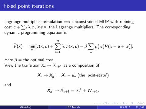
Lagrange multiplier formulation =⇒ unconstrained MDP with runningcost c +

∑i λici , λ

′i s ≈ the Lagrange multipliers. The corresponding

dynamic programming equation is

V (x) = minu

[c(x , u) +N∑i=1

λici (x , u)− β∑w

µ(w)V (x − u + w)].

Here β = the optimal cost.View the transition Xn → Xn+1 as a composition of

Xn → X+n = Xn − un (the ’post-state’)

andX+n → Xn+1 = X+

n + Wn+1.


...

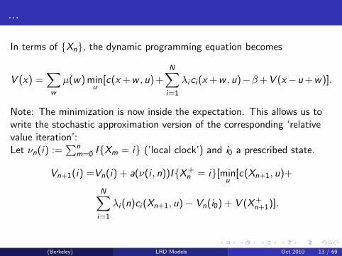
In terms of {Xn}, the dynamic programming equation becomes

V (x) =∑w

µ(w) minu

[c(x +w , u) +N∑i=1

λici (x +w , u)−β+V (x−u+w)].

Note: The minimization is now inside the expectation. This allows us towrite the stochastic approximation version of the corresponding ‘relativevalue iteration’:Let νn(i) :=

∑nm=0 I{Xm = i} (’local clock’) and i0 a prescribed state.

Vn+1(i) =Vn(i) + a(ν(i , n))I{X+n = i}[min

u[c(Xn+1, u)+

N∑i=1

λi (n)ci (Xn+1, u)− Vn(i0) + V (X+n+1)].


...

The Lagrange multipliers are updated on a slower timescale by thestochastic ascent:

λi (n + 1) = λi (n) + b(n)[ci (Xn, un)− Ci ] ∀i .

The convergence can be proved by using the two timescale analysis above.That the slow component performs the correct gradient ascent is aconsequence of the generalized envelope theorem from mathematicaleconomics.


Back to Robbins-Monro: Idea of proof:

1. Let t(0) = 0, t(n) =∑n

m=0 a(m). Then t(m) ↑ ∞.

2. Let x(t(n)) = xn with linear interpolation on [t(n), t(n + 1)](piecewise linear interpolation).

3. For s ≥ 0, let x s(t) = h(x s(t)), x s(s) = x(s).

Then if P(supn ||xn|| <∞) = 1 (i.e., iterates remain bounded withprobability one), then for T > 0,

lims↑∞

maxt∈[s,s+T ]

||x(t)− x s(t)|| = 0 w.p. 1.


Idea of proof

To prove this, use Gronwall inequality to obtain:

maxt∈[s,s+T ]

||x(t)−x s(t)|| ≤ (error due to discretization) + (error due to noise)

a(n)→ 0 =⇒ error due to discretization→ 0.

The martingale∑

n a(n)Mn+1 converges with prob. 1

=⇒ the ’tail’∑

m≥n a(m)Mm+1 goes to zero w.p. 1

=⇒ error due to noise → 0.


...

Need ’stability’: supn ||xn|| <∞ with prob. 1.

Test for stability:Let h∞(x) := lim0<a↑∞

h(ax)a .

If the origin is the globally asyptotically stable equilibrium forx(t) = h∞(x(t)), then supn ||xn|| <∞ with prob. 1.


...

martingale dierence noise {Mn}:E [Mn+1|xm,Mm,m ≤ n] = 0 =⇒ ’uncorrelated’

E [||Mn+1||2|xm,Mm,m ≤ n] ≤ K (1 + ||xn||2) =⇒ light (conditional)tails

=⇒ GOOD NOISE. In practice, noise can get BAD (long rangecorrelations) or even outright UGLY (heavy tails).

MIKOSCH, RESNICK, ROOTZEN, AND STEGEMAN characterize theregimes when one can expect these (Annals of Applied Probability, 2002)


Applications

Many DSP applications, including adaptive filtering

Network control

Adaptive routing

Service time control in queuing networks

In network applications, we wish to run control algorithms based on thevalues of the flows. However, these might not be directly observed, mightbe available as noisy estimates.It has been observed empirically that queues and flows in large computernetworks exhibit heavy tailed distributions or long range dependence.


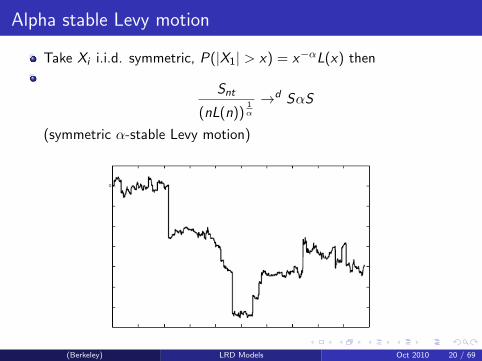
Alpha stable Levy motion

Take Xi i.i.d. symmetric, P(|X1| > x) = x−αL(x) then

Snt

(nL(n))1α

→d SαS

(symmetric α-stable Levy motion)


Alpha-stable Levy Motion properties

stationary, α-stable, i.i.d. increments.

Distribution of Snt√n→∞ (long range dependence)

Var(St) =∞Self-similarity: Snt =d n

1αSt

Samorodnitsky, Taqqu. “Stable Non-Gaussian Random Processes:Stochastic models with infinite variance”


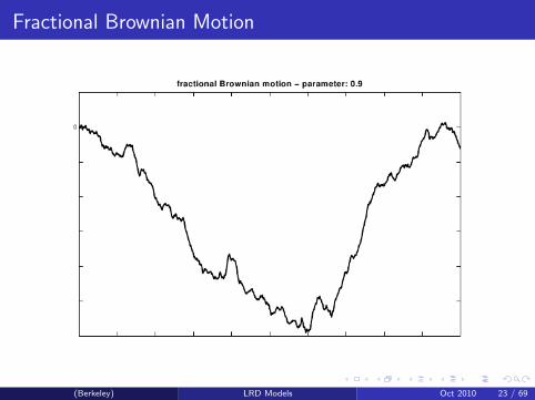
Fractional Brownian Motion

Fractional Brownian Motion is the unique Gaussian H-sssi process.

cov(BH(t1),BH(t2)) = 12{|t1|

2H + |t2|2H + |t1 − t2|2H}var(BH(1))

H-sssi

fBM limit

Let cov(X1,Xn) = n−αL(n) regularly varying. And {Xi} zero-meanGaussion.Then, Snt

nH→d BH(t), where H = (1− α

2 ).


Fractional Brownian Motion


Stochastic approximation with ’bad’ noise

Consider a stochastic approximation scheme in Rd of the type

xn+1 = xn + a(n)[h(xn) + Mn+1 + R(n)Bn+1 + D(n)Sn+1 + ξn+1],

where

Mn+1 for n ≥ 0 is the martingale difference noise as before,

Bn+1 := B(n + 1)− B(n), where B(t), t ≥ 0, is a d-dimensionalfractional Brownian motion with Hurst parameter ν ∈ (0, 1),

Sn+1 := S(n + 1)− S(n), where S(t), t ≥ 0, is a symmetric α-stableprocess with 1 < α < 2,

{ξn} is an ’error’ process satisfying supn ||ξn|| ≤ K0 <∞ a.s. andξ → 0 a.s.,


Stochastic approximation with ’bad’ noise

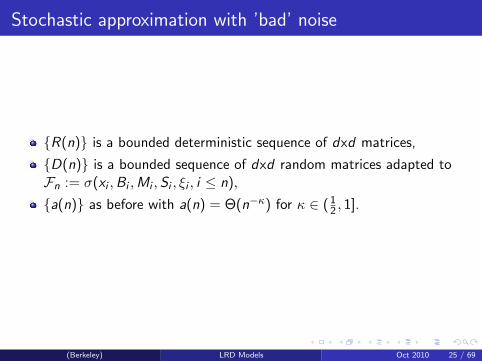
{R(n)} is a bounded deterministic sequence of dxd matrices,

{D(n)} is a bounded sequence of dxd random matrices adapted toFn := σ(xi ,Bi ,Mi , Si , ξi , i ≤ n),

{a(n)} as before with a(n) = Θ(n−κ) for κ ∈ (12 , 1].


Main theorem

Suppose that the o.d.e. x(t) = h(x(t)) has x∗ as the unique globallyasymptotically stable equilibrium and in addition, the following stabilitycondition holds:

for some ξ, 1 ≤ ξ ≤ α,supn

E [||xn||ξ] <∞.

Then for 1 < ξ′ < ξE [||xn − x∗||ξ′ ]→ 0.

(Key steps of the proof follow.)


Proof

Recall that

E [||B(t)− B(s)||2] = C |t − s|2ν , t ≥ s ≥ 0,

and for I := the identity matrix,

E [(B(t)− B(s))(B(u)− B(ν))]

=C

2

(|t − v |2ν + |s − u|2ν − |t − u|2ν − |s − v |2ν

)I ,

Then for mr (n) := min{n′ ≥ n :∑n′

i=n a(i) ≥ r} and γ := 2κ(1− ν) forν < 1

2 , := κ for ν ≥ 12 ,

E

||mt(n)∑ms(n)

a(i)R(i)B(i + 1)||2 ≤ C

nγ.


Ferniques inequality for Gaussian processes:

For p ≥ 2,K := 5√2π2 p2, γ :=

√1 + 4 log p and

φ(h) := maxs,t∈[0,1],|s−t|≤h

E [(Xt − Xs)2]12 ,

the following holds

P

(maxt∈[0,1]

|Xt | ≥[

maxx∈[0,1]

E [X 2t ]

12 + (2 +

√(2))

∫ ∞1

φ(hp−y2)dy

]x

)≤ KΨ(x).


...

Combining, these lead to: for prescribed T > 0 and

m(n) ≥ min{m ≥ n :m∑j=n

a(j) ≥ T},

we have,

E

∑n≤N≤m(n)

||N∑i=n

a(i)R(i)Bi+1||2→ 0.


Joulins inequality

P

(sup

n≤j≤m(n)||

j∑i=n

a(i)D(i)Si+1|| ≥ x

)

≤C (∑m(n)

i=n a(i)α2−1α

+1)αα+1

xα

for

x > C (

m(n)∑i=n

a(i)α2−1α

+1)αα+1 .

(A. Joulin, On maximal inequalities for stable stochastic integrals,Potential Analysis 26 (2007), pp. 57-78.) =⇒ for 0 < ξ′ < ξ,

E

∑n≤N≤m(n)

||N∑i=n

a(i)D(i)Si+1||ξ′

→ 0.


...

As before, Gronwall inequality =⇒

(Deviation from o.d.e. in ξ′th mean on an interval of length T ) ≤

(discretization error)+ (error due to martingale difference noise)+ (error due to long range dependent noise)+ (error due to heavy-tailed noise)+ (error due to {ξn})=⇒ convergence in ξ′th mean


Other results:

1. The stability test applies!

2. Concentration result for constant stepsize algorithms

3. Extension to general attractors, Markov noise, asynchronous schemes.


Markov Models with Long Range Dependence:A theorem with examples

Barlas Oguz, Venkat Anantharam

Outline

Source coding

An example from financial time series

A queuing example

TCP example


Entropy rate

Let (Xn) be a discrete-time X -valued ergodic process, X finite.

p(x1, . . . , xn) denotes P(X1 = x1, . . . ,Xn = xn).

limn

1

nE [− log p(X1, . . . ,Xn)] =: η exists,

and is called the entropy rate of the process.The logarithm is to base 2.

Write X n1 for (X1, . . . ,Xn).

In fact:η = E [− log p(X1|X 0

−∞)] .

The ergodic theorem implies:

1

n

n∑k=1

− log p(Xk |X k−1−∞ )→ η a.s.


Data compression

Let {0, 1}∗ denote the set of binary strings of finite length.

Consider a prefix-free mapping:

X n → {0, 1}∗ .

This means that no image is the prefix of any other image.

The image of xn1 is called the codeword for xn1 .

Let Ln(xn1 ) denote the length of the codeword for xn1 .

We have Kraft’s inequality:

E [2−Ln(Xn1 )] ≤ 1 .


Kraft’s inequality

Proof of Kraft’s inequality, E [2−Ln(Xn1 )] ≤ 1.


Barron’s lemma

Let {c(n)} be positive constants with∑

2−c(n) <∞.

Barron’s lemma says we have:

Ln(X n1 ) ≥ − log p(X n

1 |X 0−∞)− c(n), eventually, a.s.

A consequence, from the ergodic theorem, is that:

lim infn

Ln(X n1 )

n≥ η a.s.

This may be called a first order converse source coding theorem.


Proof of Barron’s lemma

P(Ln(X n1 ) < − log p(X n

1 |X 0−∞)− c(n)|X 0

−∞)

=∑xn1

p(xn1 |X 0−∞)1(p(xn1 |X 0

−∞) < 2−Ln(xn1 )−c(n))

≤∑xn1

2−Ln(xn1 )−c(n)1(p(xn1 |X 0

−∞) < 2−Ln(xn1 )−c(n))

≤ 2−c(n)∑xn1

2−Ln(xn1 )

≤ 2−c(n) .


Second order source coding theorems

By Barron’s lemma, we have:

Ln(X n1 )− n η ≥

[n∑

k=1

− log p(Xk |X k−1−∞ )− n η

]− c(n)

eventually a.s. for any sequence of positive constants with∑

2−c(n) <∞.

Thus, if (Xn) is a sufficiently fast mixing process (e.g. a finite-order Markovchain), then

lim infn

Lbntc − ntη

n1/2≥Wt

where Wt is a scaled Brownian motion.

This is the second order converse source coding theorem of Kontoyiannis,1997.

For finite-order Markov chains, or if one has sufficiently strong mixing for

maxx1

E | log p(x1|X 0−n+1)− log p(x1|X 0

−∞)| ,

a matching second order direct source coding theorem holds for mostreasonable codes, e.g. Shannon codes, Huffman codes or Lempel-Ziv codes.


Aim of this talk

We are motivated by the empirical observation of long-rangedependence in variable bit rate video traffic, starting with Garrett andWillinger, 1994 and Beran, Sherman, Taqqu, and Willinger, 1995.

We ask:What happens when (Xn) is a long-range dependent process?Specifically:Can we find a codec to make (Ln) short-range dependent?

Loosely speaking, we propose the answer: No.

More precisely, we prove a theorem about long-range-dependentrenewal processes that says: No.


Long-range-dependent renewal processes

Known facts from Daley, 1999

Let (Xn) be a renewal process with interarrival times having thedistribution of T . Then, for 1 < p < 2, the following statements areequivalent:

i T has moment index p.

ii (Xn) has Hurst index H = 12(3− p).

Here, the moment index of T is defined by:

p = sup{κ ≥ 1 : E [Tκ] <∞} ,

and a stationary ergodic process (Zn) with E [Z 20 ] <∞ is said to have

Hurst index H if:

H = inf{h : limsupnvar(

∑nk=1 Zk)

n2h<∞} .


Main theorem

Let ρn denote − log p(Xn|X n−1−∞ ).

We show that E [ρ2n] <∞ and that (ρn) has the same Hurst index as(Xn).By Barron’s lemma, this, in principle, gives second-order conversesource coding theorems for long-range-dependent renewal processes.

Main theorem

Let (Xn) be a renewal process with interarrival times having thedistribution of T . Then, for 1 < p < 2, the following statements areequivalent:

i T has moment index p.ii (Xn) has Hurst index H = 1

2(3− p).iii (ρn) has Hurst index H = 1

2(3− p).


The question of interest for Markov chains

For a countable state stationary ergodic Markov chain, if any returntime has infinite variance, then all return times have the samemoment index (Carpio & Daley, 2007).

For such a chain, we say it has Hurst index H if a (any) return timehas moment index corresponding to Hurst index H.

Our question is of the type:When does an instantaneous function of such a Markov chain havethe same Hurst index as the chain?

An example for which this fails (Carpio & Daley 2007):Let M3

n = (M1n ,M

2n) ∈ S1xS2. where (M1

n) has Hurst index12 < H < 1, while (M2

n) has return times with finite variance. Then(M3

n) will inherit the Hurst index of (M1n). However, instantaneous

functions of Mn3 that only depend on M2

n will produce processes withHurst index 1

2 .


The relevant facts from Carpio & Daley

Carpio & Daley, 2007

var(ρ0 + . . .+ ρn)− (n + 1)var(ρ0)

2R(n)11 /π1

=∑i

∑j

ρ(i)ρ(j)πiπjR(n)ij /πj

R(n)11 /π1

πi denotes the stationarydistribution of state i

Q(n)ij :=

∑nr=1(p

(r)ij − πj)

R(n)ij :=

∑nr=1Q

(r)ij

Q(n)ij →∞

R(n)ij

n →∞R

(n)ij /πj

R(n)11 /π1

→ 1

limnvar(ρ0+...+ρn)

2R(n)11 /π1

?=∑

i

∑j ρ(i)ρ(j)πiπj


One theorem

Let

(condition 1)

limn→∞

1

Q(n)11 /π1

n∑r=1

∑i ,j

πi (ρ(i)− c)(ρ(j)− c)1p(r)ij = 0

for some constant c , and(condition 2)

limL→∞

limn→∞

1

Q(n)11 /π1

n∑r=1

∑i ,j

πi |ρ(i)ρ(j)|1(|ρ(i)|, |ρ(j)| > L)1p(r)ij = 0

Then,

limn→∞

var(∑n

r=1 ρi )

R(n)11 /π1

= (µ− c)2

Moreover, if c 6= µ, then Hρ = H.(Berkeley) LRD Models Oct 2010 46 / 69

One theorem

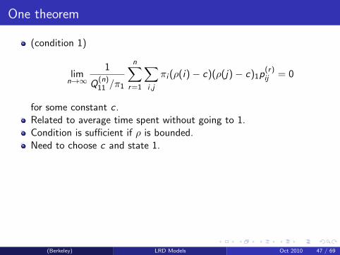
(condition 1)

limn→∞

1

Q(n)11 /π1

n∑r=1

∑i ,j

πi (ρ(i)− c)(ρ(j)− c)1p(r)ij = 0

for some constant c .Related to average time spent without going to 1.Condition is sufficient if ρ is bounded.Need to choose c and state 1.


One theorem

(condition 2)

limL→∞

limn→∞

1

Q(n)11 /π1

n∑r=1

∑i ,j

πi |ρ(i)ρ(j)|1(|ρ(i)|, |ρ(j)| > L)1p(r)ij = 0

Needed when ρ is not bounded.Implied by

1

Q(n)11 /π1

∑i ,j

πi |ρ(i)− c ||ρ(j)− c |n∑

r=1

1p(r)ij → 0


One theorem

limn→∞

var(∑n

r=1 ρi )

R(n)11 /π1

= (µ− c)2

Moreover, if c 6= µ, then Hρ = H.

H is calculated from the moment index of the return time distribution.


Useful lemma

Let {Ak}, 1 ≤ k ≤ K , be a finite partition of the state space N.(condition 1) Let

limn→∞

1

Q(n)11

∑i∈Ak ,j∈Al

|ρ(i)− µ|πi |ρ(j)− µ|n∑

r=1

1p(r)ij → 0 ∀k 6= l

And suppose π∞Ak:= limn→∞

∑i∈Ak

πi∑n

r=1 1p(r)ij∑

i πi∑n

r=1 1p(r)ij

exists ∀k.

Then the lemma says, we can treat each subset separately.


Useful lemma

If there exists constants ck , 1 ≤ k ≤ K such that

(condition 2)

limn→∞

1

Q(n)11 /π1

n∑r=1

∑i ,j∈Ak

πi (ρ(i)− ck)(ρ(j)− ck)1p(r)ij = 0 ∀k

for constants (ck), and(condition 3)

limL→∞

limn→∞

1

Q(n)11 /π1

n∑r=1

∑i ,j∈Ak

πi |ρ(i)ρ(j)|1(|ρ(i)|, |ρ(j)| > L)1p(r)ij = 0 ∀k

Then,

limn→∞

var(∑n

r=1 ρi )

R(n)11 /π1

=K∑

k=1

π∞Ak(µ− ck)2

Moreover, if π∞Ak(ck − µ) 6= 0, then Hρ = H.


Applying the theorem to a renewal process

ρ(0) = − logP(T = 1).

ρ(2k − 1) = − logP(T > k |T ≥k).

ρ(2k) = − logP(T = k + 1|T ≥k + 1).

π(2k) = P(T=k+1)E [T ] ,

k = 0, 1, 2, . . ..

π(2k − 1) = P(T≥k+1)E [T ] ,

k = 1, 2, . . ..

We can show that∑

i π(i)ρ(i)2 <∞.


Applying the theorem to a renewal process

Consider the basic renewal process (Xn) with P(T > k) = k−αL(k).1 < α < 2, where L(k) is slowly varying.

Then ρ(i)→ 0 when moving through the odd states

However, ρ(i)→∞ when moving through the even states.

1pij = 0 in this case, so the condition holds.


Financial time series

rn = log PnPn−1

, is called the log returns, where Pn is the price of someasset.

rn is well modeled by a Martingale difference process, due to theefficient market hypothesis.

The absolute returns |rn|d have been empirically shown to exhibitlong memory.


Mandelbrot’s model for wheat prices

Can a simple model account forthis observation?

Mandelbrot’s model for wheatprices

Weather has runs ofgood/neutral/bad days.

Good/bad period is followed byneutral period (and visa versa)

The ‘fundamental price’, Xn,increases by 1 on good days,decreases by 1 on bad days,unaltered on neutral days.



Distribution of length of eachperiod f (T > t) = t−α

Market calculatesXn = limt→∞ E [Xn+t |X n−1

−∞ ].

By construction Xn is aMartingale.



Xn changes as follows: increasesby α

α−1 for every good day,

Decreases by αα−1 for every bad

day.

The first neutral following tgood days decreases Xn by t

α−1 .

The first neutral following t baddays increases Xn by t

α−1 .

The price is unchanged for thefollowing neutral days.


The Markov chain

The weather can be modeled asa MC.

The differences in fundamentalprice is a function of this chain(Good = ‘1’, Bad=‘-1’,Neutral=‘0’)


The Markov chain

For the Market price returns(rn), we need to also knowwhere we jumped from.

rn takes values ± αα−1 , 0,±

tα−1 ,

where t the in number of dayspreceding the jump.

What is the Hurst index of |rn|d?


Queuing example

X1 i.i.d. with heavy tails.

X2 i.i.d. with light tails (or a SRD Markov process)

Server has unit capacity


LRD behavior under LQF

Let M1,M2 be MCs representingthe two sources.

(M1(n),M2(n),Q1(n),Q2(n)) isa MC (under any queue lengthbased scheduling).

Busy-idle function 1(Q1(n) = 0)is LRD.

Is 1(Q2(n) = 0) LRD under LQF?


TCP example

Let rs(n) be the rate under TCP.

rl(n) is the traffic across critical link (in the absense of rs).

Packets are dropped whenever rs + rl > Cl .


TCP example

rs incremented when there is nodrop (upto rmax). rs halvedwhen there is a drop.

Assume rl is modeled by LRDMarkov chain.

(rs , rl) is a Markov chain.

What is the Hurst index of rs?


Solution: financial time series

State 1 (red).



State 1 (red).

c1 = 0, c2 = αα−1 , c3 = 0

In groups 1,2, ρ− ck = 0. Ingroup 3, 1pij = 0. (all returnsare through state 1).

Therefore the condition

limn→∞

1

Q(n)11 /π1

n∑r=1

∑i ,j∈Ak

πi |(ρ(i)− ck)(ρ(j)− ck)|1p(r)ij = 0 ∀k

is satisfied.



We get

limn→∞

var(∑n

r=1 ρi )

R(n)11 /π1

=2

3(µ− α

α− 1)2 +

1

3µ2 > 0

for any d for which |rn|d has finite variance. (d < α/2)

|rn|d has Hurst index H = 12(3− α).


Solution: LQF scheduling

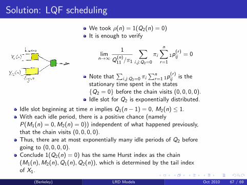
We took ρ(n) = 1(Q2(n) = 0)It is enough to verify

limn→∞

1

Q(n)11 /π1

∑i ,j :Q2=0

πi

n∑r=1

1p(r)ij = 0

Note that∑

i ,j :Q2=0 πi∑n

r=1 1p(r)ij is the

stationary time spent in the states{Q2 = 0} before the chain visits (0, 0, 0, 0).Idle slot for Q2 is exponentially distributed.

Idle slot beginning at time n implies Q1(n − 1) = 0, M2(n) ≤ 1.With each idle period, there is a positive chance (namelyP(M1(n) = 0,M2(n) = 0)) independent of what happened previously,that the chain visits (0, 0, 0, 0).Thus, there are at most exponentially many idle periods of Q2 beforegoing to (0, 0, 0, 0).Conclude 1(Q2(n) = 0) has the same Hurst index as the chain(M1(n),M2(n),Q1(n),Q2(n)), which is determined by the tail indexof X1.


Solution: TCP

A simple (unrealistic) model for rl : on-off process (on = Cl , off=0)with heavy tailed intervals.

Divide state space into two: A1 = {rl = 0},A2 = {rl = Cl}ρ = rs .

Choose c1 = rmax , c2 = 0.

On A1, rs = rmax after a finite number of states.

Similarly on A2, rs = 0 after a finite number of states.


Solution: TCP

Therefore the condition

limn→∞

1

Q(n)11 /π1

n∑r=1

∑i ,j∈Ak

πi |(ρ(i)− ck)(ρ(j)− ck)|1p(r)ij = 0 ∀k

is satisfied.

Remains to check the condition for the lemma.

rs inherits the Hurst index of rl .


Documents

Models with Long Range Dependence and Heavy Tailsrobotics.eecs.berkeley.edu/~wlr/ADCN-slides/review1010/Anantharam.pdfModels with Long Range Dependence and Heavy Tails Vivek S. Borkar1