Embed Size (px)
Citation preview
HAL Id: ensl-00356709https://hal-ens-lyon.archives-ouvertes.fr/ensl-00356709v3
Submitted on 27 May 2010
HAL is a multi-disciplinary open accessarchive for the deposit and dissemination of sci-entific research documents, whether they are pub-lished or not. The documents may come fromteaching and research institutions in France orabroad, or from public or private research centers.
L’archive ouverte pluridisciplinaire HAL, estdestinée au dépôt et à la diffusion de documentsscientifiques de niveau recherche, publiés ou non,émanant des établissements d’enseignement et derecherche français ou étrangers, des laboratoirespublics ou privés.
The functions erf and erfc computed with arbitraryprecision and explicit error bounds
Sylvain Chevillard
To cite this version:Sylvain Chevillard. The functions erf and erfc computed with arbitrary precision and explicit errorbounds. Information and Computation, Elsevier, 2012, 216, pp.72 – 95. �ensl-00356709v3�
Laboratoire de l’Informatique du Parallélisme
École Normale Supérieure de Lyon
Unité Mixte de Recherche CNRS-INRIA-ENS LYON-UCBL no 5668
The functions erf and erfc computed with
arbitrary precision
Sylvain ChevillardJanuary 2009 -May 2010
Research Report No RR2009-04
École Normale Supérieure de Lyon46 Allée d’Italie, 69364 Lyon Cedex 07, France
Téléphone : +33(0)4.72.72.80.37Télécopieur : +33(0)4.72.72.80.80
Adresse électronique : [email protected]
ENSDE LYON
The functions erf and erfc computed with arbitrary precision
Sylvain Chevillard
January 2009 - May 2010
Abstract
The error function erf is a special function. It is widely used in statisticalcomputations for instance, where it is also known as the standard normalcumulative probability. The complementary error function is defined aserfc(x) = 1− erf(x).In this paper, the computation of erf(x) and erfc(x) in arbitrary precisionis detailed: our algorithms take as input a target precision t′ and deliverapproximate values of erf(x) or erfc(x) with a relative error guaranteedto be bounded by 2−t
′
.We study three different algorithms for evaluating erf and erfc. Thesealgorithms are completely detailed. In particular, the determinationof the order of truncation, the analysis of roundoff errors and the wayof choosing the working precision are presented. The scheme used forimplementing erf and erfc and the proofs are expressed in a generalsetting, so they can directly be reused for the implementation of otherfunctions.We have implemented the three algorithms and studied experimentallywhat is the best algorithm to use in function of the point x and thetarget precision t′.
Keywords: Error function, complementary error function, erf, erfc, floating-pointarithmetic, arbitrary precision, multiple precision.
Resume
La fonction d’erreur erf est une fonction speciale. Elle est courammentutilisee en statistiques par exemple. La fonction d’erreur complementaireest definie comme erfc(x) = erf(x)− 1.Dans cet article, nous detaillons l’evaluation de erf(x) et erfc(x) en preci-sion arbitraire : nos algorithmes prennent en entree une precision cible t′
et fournissent en retour une valeur approchee de erf(x) ou erfc(x) avecune erreur relative bornee par 2−t
′
.Nous etudions trois algorithmes differents pour evaluer erf et erfc. Ces al-gorithmes sont expliques en details. En particulier, nous decrivons com-ment determiner l’ordre de troncature, comment analyser les erreursd’arrondi et comment choisir la precision intermediaire de travail. Leschema employe pour l’implantation de erf et erfc est explique en destermes generaux et peut donc etre directement reutilise pour l’implan-tation d’autres fonctions.Nous avons implemente les trois algorithmes ; nous concluons par uneetude experimentale qui montre quel algorithme est le plus rapide enfonction du point x et de la precision cible t′.
Mots-cles: fonctions d’erreur, erf, erfc, arithmetique flottante, precision arbitraire,multiprecision
2
erf and erfc in arbitrary precision 1
1 Introduction
The error function, generally denoted by erf is defined as
erf : x 7→ 2√π
∫ x
0e−v
2
dv.
Sometimes it is called the probability integral [12], in which case, erf denotes the integral itselfwithout the normalization factor 2/
√π. The complementary error function denoted by erfc is
defined as erfc = 1− erf. These two functions are defined and analytic on the whole complexplane. Nevertheless we will consider them only on the real line herein.
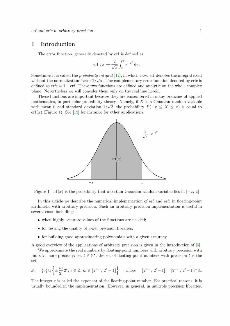
These functions are important because they are encountered in many branches of appliedmathematics, in particular probability theory. Namely, if X is a Gaussian random variablewith mean 0 and standard deviation 1/
√2, the probability P (−x ≤ X ≤ x) is equal to
erf(x) (Figure 1). See [12] for instance for other applications.
Figure 1: erf(x) is the probability that a certain Gaussian random variable lies in [−x, x]
In this article we describe the numerical implementation of erf and erfc in floating-pointarithmetic with arbitrary precision. Such an arbitrary precision implementation is useful inseveral cases including:
❼ when highly accurate values of the functions are needed;
❼ for testing the quality of lower precision libraries;
❼ for building good approximating polynomials with a given accuracy.
A good overview of the applications of arbitrary precision is given in the introduction of [5].We approximate the real numbers by floating-point numbers with arbitrary precision with
radix 2; more precisely: let t ∈ N⋆, the set of floating-point numbers with precision t is theset
Ft = {0}∪{± m
2t2e, e ∈ Z, m ∈ J2t−1, 2t − 1K
}where J2t−1, 2t−1K = [2t−1, 2t−1]∩Z.
The integer e is called the exponent of the floating-point number. For practical reasons, it isusually bounded in the implementation. However, in general, in multiple precision libraries,
2 S. Chevillard
its range is extremely large (typically e ∈ [−232; 232]) and may be considered as practicallyalmost unbounded. We will assume in this paper that e is unbounded. The number m/2t
is called the mantissa and is more conveniently written as 0.1b2 . . . bt where b2, . . . , bt arethe bits of its binary representation. The mantissa lies in the interval [1/2, 1): this is theconvention used by the MPFR library and we will adopt it here. Note that the IEEE-754standard takes another convention and suppose that the mantissa lies in [1, 2).
Our goal is the following: given t′ in N⋆ and x a floating-point number, compute a valuey approximating erf(x) with a relative error less than 2−t
′
. More formally, we would like tocompute y such that
∃δ ∈ R, y = erf(x)(1 + δ) where |δ| ≤ 2−t′
.
Arbitrary precision floating-point arithmetic is already implemented in several softwaretools and libraries. Let us cite Brent’s historical Fortran MP package [4], Bailey’s Arprec C++library [2], the MPFR library [9], and the famous Mathematica and Maple tools. MPFR providescorrect rounding of the functions: four rounding-modes are provided (rounding upwards,downwards, towards zeros, and to the nearest) and the returned value y is the rounding ofthe exact value erf(x) to the target precision t′. Other libraries and tools usually only ensurethat the relative error between y and the exact value is O(2−t
′
).
Our implementation guarantees that the final relative error be smaller than 2−t′
. This isstronger than O(2−t
′
), since the error is explicitly bounded.
Since we provide an explicit bound on the error, our implementation can also be used toprovide correct rounding, through an algorithm called Ziv’s onion strategy [15]: in order toobtain the correct rounding in precision t′, a first approximate value is computed with a fewguard bits (for instance 10 bits). Hence | erf(x) − y| ≤ 2−t
′−10 erf(x). Most of the time, itsuffices to round y to t′ bits in order to obtain the correct rounding of erf(x). But in rare cases,this is not true and another value y must be computed with more guard bits. The precisionis increased until the correct rounding can be decided. This is the strategy used by MPFR
for instance. Providing correct rounding does not cost more in average than guaranteeing anerror smaller than 2−t
′
: the average complexity of Ziv’ strategy is the complexity of the firststep, i.e. when only 10 guard bits are used.
For our implementation, we use classical formulas for approximating erf and erfc and weevaluate them with a summation technique proposed by Smith [14] in 1989. As we alreadymentioned, some implementations of erf and erfc are already available. However:
❼ None of them uses Smith’s technique. This technique allows us to have the most efficientcurrently available implementation.
❼ In general they use only one approximating method. In this article, we study threedifferent approximating formulas and show how to heuristically choose the most efficientone, depending on the target precision and the evaluation point.
❼ Most of the available implementations do not guarantee an explicit error bound. TheMPFR library actually does give an explicit error bound. However, only few details aregiven on the implementation of functions in MPFR. The only documentation on MPFR isgiven by [9] and by the file algorithm.pdf provided with the library. In general, thereis no more than one or two paragraphs of documentation per function.
erf and erfc in arbitrary precision 3
❼ More generally, to our best knowledge, there does not exist any reference article de-scribing in detail how to implement a function in arbitrary precision, with guaranteederror bounds. In this article, we explicitly explain how to choose the truncation rankof each formula, how to perform the roundoff analysis and how to choose the workingprecision used for the intermediate computations. Through the detailed example of thefunctions erf and erfc, this article gives a general scheme that can be followed for theimplementation of other functions.
Our implementation is written in C and built on top of MPFR. It is distributed under the LGPLand it is available with this research report at http://prunel.ccsd.cnrs.fr/ensl-00356709/.
The outline of the paper is as follows: Section 2 begins with a general overview of thescheme used to evaluate functions in arbitrary precision by means of series. The sectioncontinues with a general discussion about erf and erfc and the ways of computing them witharbitrary precision. In particular, the algorithm used for the evaluation of the series is detailed.Section 3 is devoted to some reminders on classical techniques required for performing theroundoff analysis. In Section 4 the algorithms are completely described and the roundoffanalysis is detailed. However, for the sake of clarity, proofs are omitted in that section. Theyare all given in an appendix at the end of the article. Section 5 gives experimental results.In particular, it gives timings comparing our implementation with MPFR and Maple. It alsoexperimentally shows what is the best approximating method, depending on the evaluationpoint and the target precision. Finally, Section 6 is devoted to the conclusion and presentsfuture works.
2 General overview of the algorithms
2.1 General scheme used for the evaluation in arbitrary precision
In order to evaluate a function f in arbitrary precision, it is necessary to have approxi-mating formulas that can provide values arbitrarily close to the exact value f(x). We referto [5] for a general overview of the classical techniques in this domain. In the following, weshall restrict to the case when a power series or an asymptotic series is used.
Let us assume for instance that f(x) =∑+∞n=0 an x
n. Two important questions must beaddressed:
❼ In practice, only a finite number N of terms are summed (so the truncation rank isN − 1). We must choose N in such a way that the approximation error be smallenough.
❼ Floating-point arithmetic is used when evaluating the sum. This implies that roundingerrors affect the final result. In order to keep this evaluation error small enough, theworking precision should be carefully chosen.
In particular, it is important to distinguish the target precision (i.e. the value t′ such thatwe eventually want to return an approximate value y satisfying |y − f(x)| ≤ 2−t
′ |f(x)|) andthe working precision (i.e. the precision used to perform the computations). In the following,we will always denote by t the working precision.
We adopt the following strategy for the implementation of f :
1. Find a rough overestimation N − 1 of the truncation rank.
4 S. Chevillard
2. Rigorously bound the roundoff errors. This allows us to choose a suitable workingprecision.
3. Evaluate the series. An on-the-fly criterion allows us to stop the evaluation as soon aspossible. So, in practice, the finally used truncation rank N⋆ − 1 is near-optimal.
A few remarks are necessary to understand this strategy. First, we remark that theroundoff errors depend on several things: the series used (the values an may be more orless complicated to evaluate), the evaluation scheme used to evaluate the series, and thenumber of operations performed. This is why we need to have an overestimation N − 1 ofthe truncation rank before we choose the working precision. However, this estimation doesnot need to be very accurate, since (as we will see) only the logarithm of N matters for theroundoff errors. Of course, in practice we do not want to perform more operations than whatis strictly necessary: this is why we use an on-the-fly stopping criterion at step 3.
We want that the final absolute error be smaller than 2−t′ |f(x)|. In practice, we cut this
error into two equal parts: we choose the truncation rank and the working precision in such away that both the approximation error and the evaluation error be smaller than 2−t
′−1 |f(x)|.The overall error is bounded by the sum of both errors, which gives the desired bound.
Since we want to ensure that the value N be an overestimation, it must be determinedwith care. It is generally possible to bound the remainder of order N , in function of x: i.e.we usually explicitly know a function εN such that
∀x,∣∣∣∣∣f(x)−
N−1∑
n=0
ai xi
∣∣∣∣∣ ≤ εN (x).
Hence it suffices to choose N such that εN (x) ≤ 2−t′−1 |f(x)|. The problem is that we do not
know |f(x)| yet. Thus, for finding N we must address two problems:
❼ Find an easily computable underestimation g(x) of |f(x)|.
❼ Find N such that we are sure that εN (x) ≤ 2−t′−1 g(x). This implies inverting the
function N 7→ εN (x).
The scheme that we just described is general and can be used for the implementation ofother functions. Let us sum up the questions that must be addressed:
1. Find one (or several) series∑+∞n=0 an x
n approximating f(x). It can also be an asymptoticdevelopment.
2. Choose an algorithm for the evaluation of this series.
3. Perform a roundoff analysis of this algorithm. This gives an error bound that dependson the truncation rank.
4. Find a good underestimation g(x) of |f(x)|.
5. Find a good bound εN (x) of the remainder of the series, and invert the relation εN (x) ≤2−t
′−1 g(x) in function of N .
Provided that these questions find an answer, our technique applies. In the following, we willanswer these questions in the case when f = erf or f = erfc. More precisely:
erf and erfc in arbitrary precision 5
❼ We give three approximating series for erf and erfc in the next Section 2.2.
❼ We describe evaluation algorithms in Section 2.3. These algorithms are not specific to erfor erfc and can be reused in other contexts. The actual algorithms used for evaluatingerf and erfc are described in Section 4 and more precisely in Figures Algorithm 3,Algorithm 4 and Algorithm 5.
❼ We show how to perform a roundoff analysis in Section 3. Again, this section is generaland can be reused in other contexts. The specific roundoff analyses of our implementa-tion are given in Propositions 4, 6 and 8.
❼ We give explicit underestimations of | erf(x)| and | erfc(x)| in the appendix in Lemma 9.
❼ We give explicit bounds for the remainder of the series that we use for the implemen-tation of erf and erfc and show how to invert them. This gives us a rough but rigorousoverestimation of the necessary truncation rank for each approximation formula. Theseresults are summed up in Recipes 1, 3 and 5.
❼ Finally, we use our roundoff analyses together with the estimations of the truncationranks, in order to choose a suitable working precision t for each approximation formula.These results are summed up in Recipes 2, 4 and 6.
2.2 Approximation formulas for erf and erfc
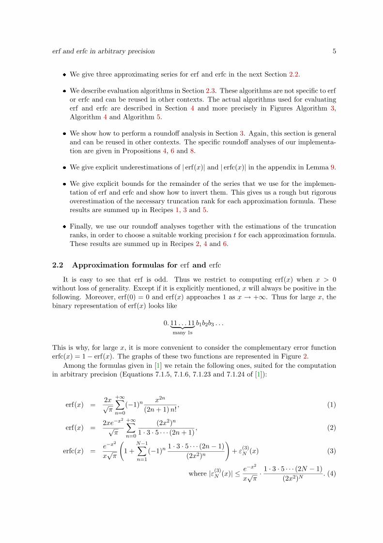
It is easy to see that erf is odd. Thus we restrict to computing erf(x) when x > 0without loss of generality. Except if it is explicitly mentioned, x will always be positive in thefollowing. Moreover, erf(0) = 0 and erf(x) approaches 1 as x → +∞. Thus for large x, thebinary representation of erf(x) looks like
0. 11 . . . 11︸ ︷︷ ︸many 1s
b1b2b3 . . .
This is why, for large x, it is more convenient to consider the complementary error functionerfc(x) = 1− erf(x). The graphs of these two functions are represented in Figure 2.
Among the formulas given in [1] we retain the following ones, suited for the computationin arbitrary precision (Equations 7.1.5, 7.1.6, 7.1.23 and 7.1.24 of [1]):
erf(x) =2x√π
+∞∑
n=0
(−1)nx2n
(2n+ 1)n!, (1)
erf(x) =2xe−x
2
√π
+∞∑
n=0
(2x2)n
1 · 3 · 5 · · · (2n+ 1), (2)
erfc(x) =e−x
2
x√π
(1 +
N−1∑
n=1
(−1)n1 · 3 · 5 · · · (2n− 1)
(2x2)n
)+ ε
(3)N (x) (3)
where |ε(3)N (x)| ≤ e
−x2
x√π· 1 · 3 · 5 · · · (2N − 1)
(2x2)N. (4)
6 S. Chevillard
(a) Graph of erf (b) Graph of erfc
Figure 2: Graphs of the functions erf and erfc
These formula can also be rewritten, with a more compact form, using the symbol 1F1 ofhypergeometric functions:
1F1(a, b; x) =+∞∑
i=0
a (a+ 1) . . . (a+ n− 1)xn
b (b+ 1) . . . (b+ n− 1) (n!).
So, we have
erf(x) =2x√π
1F1
(1
2,
3
2; −x2
)(1′ )
and erf(x) =2xe−x
2
√π
1F1
(1,
3
2; x2
). (2′ )
Equation (1) is mostly interesting for small values of x. The series is alternating and theremainder is thus bounded by the first neglected term. The ratio between two consecutiveterms is, roughly speaking, x2/n. Thus, if x < 1, both x2 and n contribute to reducethe magnitude of the term and the convergence is really fast. For larger values of x, theconvergence is slower since only the division by n ensures that the term decreases. Though,the main problem with large arguments is not the speed of the convergence.
The main drawback of (1) for large arguments comes from the fact that the series isalternating: the sum is henceforth ill-conditioned and accuracy is lost during the evaluation.This is due to a phenomenon usually called catastrophic cancellation [8].
Definition 1 (Cancellation). Let a and b be two numbers. When subtracting b from a, wesay that there is a cancellation of bits when the leading bits of a and b cancel out. In this case,only the last (few) bits of a and b contribute to the result. Thus, the accuracy of the resultcan be much smaller than the accuracy of a and b.
Due to this cancellation phenomenon, the computations must be performed with a preci-sion much higher than the target precision. We will quantify this phenomenon in Section 4.2:as we will see, as x increases, the use of Equation (1) quickly becomes impractical.
Equation (2) does not exhibit cancellations. Its evaluation does not require much moreprecision than the target precision. However, the convergence is a bit slower. Besides, it
erf and erfc in arbitrary precision 7
requires to compute e−x2
(the complexity of computing it is somewhat the same as computingerf itself).
Equation (3) gives a very efficient way of evaluating erfc and erf for large arguments.
However ε(3)N (x) cannot be made arbitrarily small by increasing N (there is an optimal value
reached when N = ⌊x2 + 1/2⌋). If erfc(x) is to be computed with a bigger precision, one hasto switch back to Equation (1) or (2).
2.3 Evaluation scheme
2.3.1 Particular form of the sums
The three sums described above exhibit the same general structure: they are polynomialsor series (in the variable x2, 2x2 or 1/(2x2)) with coefficients given by a simple recurrenceinvolving multiplications or divisions by integers. More formally, they can all be written as
S(y) = α0 + α0α1 y + . . .+ α0α1 · · ·αN−1 yN−1. (5)
Namely, we have
❼ in the case of Equation (1), y = −x2, α0 =2x√π
and for i ≥ 1, αi =2i− 1
(2i+ 1) i;
❼ in the case of Equation (2), y = 2x2, α0 =2xe−x
2
√π
and for i ≥ 1, αi =1
2i+ 1;
❼ in the case of Equation (3), y =−1
2x2, α0 =
e−x2
x√π
and αi = 2i− 1.
It is important to remark that the values αi are integers (or inverse of integers) that fitin a 32-bit or 64-bit machine integer. The multiplication (or division) of a t-bit floating-point number by a machine integer can be performed [4] in time O(t). This should becompared with the multiplication of two t-bit floating-point numbers which is performed intime O(t log(t) log(log(t))) asymptotically (and which is only quadratic for small precisions).Additions and subtractions of two t-bit floating-point numbers are also done in time O(t).
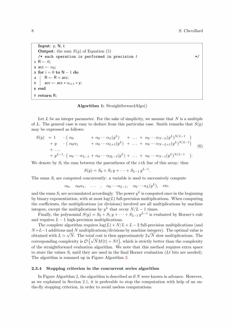
2.3.2 Straightforward algorithm
A natural way of evaluating the sum (5) is to successively compute the terms of the sum,while accumulating them in a variable (see Algorithm 1).
With this algorithm the following operations are performed: N additions, N multiplica-tions by the small integers αi+1, and N full-precision multiplications by y. The total cost ofthe algorithm is henceforth dominated by the full-precision multiplications: the complexity isO(N M(t)) where M(t) denotes the cost of a full-precision multiplication in precision t.
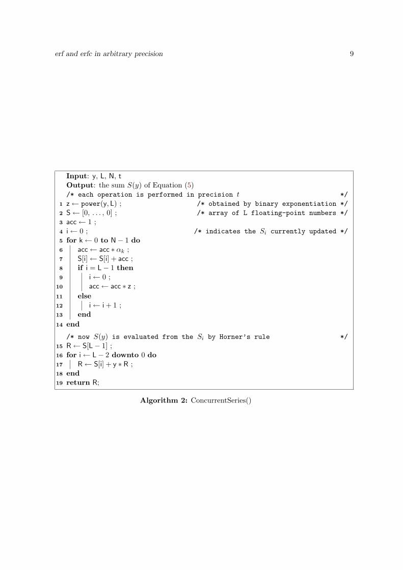
2.3.3 Concurrent Series Algorithm
We may take advantage of the particular structure of the sum (5), using a techniquedescribed by Smith [14] as a concurrent series summation (after an idea of Paterson andStockmeyer [13]).
8 S. Chevillard
Input: y, N, t
Output: the sum S(y) of Equation (5)/* each operation is performed in precision t */
R← 0;1
acc← α0;2
for i = 0 to N− 1 do3
R← R + acc;4
acc← acc ∗ αi+1 ∗ y;5
end6
return R;7
Algorithm 1: StraightforwardAlgo()
Let L be an integer parameter. For the sake of simplicity, we assume that N is a multipleof L. The general case is easy to deduce from this particular case. Smith remarks that S(y)may be expressed as follows:
S(y) = 1 ·(α0 + α0 · · ·αL(yL) + . . . + α0 · · ·αN−L(yL)N/L−1
)
+ y ·(α0α1 + α0 · · ·αL+1(yL) + . . . + α0 · · ·αN−L+1(yL)N/L−1
)
+ . . .
+ yL−1·(α0 · · ·αL−1 + α0 · · ·α2L−1(yL) + . . . + α0 · · ·αN−1(yL)N/L−1
).
(6)
We denote by Si the sum between the parentheses of the i-th line of this array: thus
S(y) = S0 + S1 y + · · ·+ SL−1 yL−1.
The sums Si are computed concurrently: a variable is used to successively compute
α0, α0α1, . . . , α0 · · ·αL−1, α0 · · ·αL(yL), etc.
and the sums Si are accumulated accordingly. The power yL is computed once in the beginningby binary exponentiation, with at most log(L) full-precision multiplications. When computingthe coefficients, the multiplications (or divisions) involved are all multiplications by machineintegers, except the multiplications by yL that occur N/L− 1 times.
Finally, the polynomial S(y) = S0 + S1 y + · · ·+ SL−1 yL−1 is evaluated by Horner’s rule
and requires L− 1 high-precision multiplications.The complete algorithm requires log(L) +N/L+L− 2 full-precision multiplications (and
N+L−1 additions andN multiplications/divisions by machine integers). The optimal value isobtained with L ≃
√N . The total cost is then approximately 2
√N slow multiplications. The
corresponding complexity is O(√NM(t) +Nt
), which is strictly better than the complexity
of the straightforward evaluation algorithm. We note that this method requires extra spaceto store the values Si until they are used in the final Horner evaluation (Lt bits are needed).The algorithm is summed up in Figure Algorithm 2.
2.3.4 Stopping criterion in the concurrent series algorithm
In Figure Algorithm 2, the algorithm is described as ifN were known in advance. However,as we explained in Section 2.1, it is preferable to stop the computation with help of an on-the-fly stopping criterion, in order to avoid useless computations.
erf and erfc in arbitrary precision 9
Input: y, L, N, t
Output: the sum S(y) of Equation (5)/* each operation is performed in precision t */
z← power(y, L) ; /* obtained by binary exponentiation */1
S← [0, . . . , 0] ; /* array of L floating-point numbers */2
acc← 1 ;3
i← 0 ; /* indicates the Si currently updated */4
for k← 0 to N− 1 do5
acc← acc ∗ αk ;6
S[i]← S[i] + acc ;7
if i = L− 1 then8
i← 0 ;9
acc← acc ∗ z ;10
else11
i← i + 1 ;12
end13
end14
/* now S(y) is evaluated from the Si by Horner’s rule */
R← S[L− 1] ;15
for i← L− 2 downto 0 do16
R← S[i] + y ∗ R ;17
end18
return R;19
Algorithm 2: ConcurrentSeries()
10 S. Chevillard
In Figure Algorithm 2, the terms of Equation (6) are computed successively beginningby the first column (from top to bottom), following by the second column (from top tobottom), etc. The variable k denotes the term currently being computed, while the variablei represents the corresponding line. The variable acc is used to store the current term: justafter the line 6 of the algorithm was performed, (acc ·yi) is an approximation to the k-th termof the polynomial S(y).
This means that N does not really need to be known in advance: a test of the formsum the terms until finding one whose absolute value is smaller than a given bound can beused. Of course, (acc · yi) is only an approximation of the actual coefficient. If we are notcareful enough, we might underestimate the absolute value and stop the summation too soon.Hence, the rounding mode should be chosen carefully when updating acc, in order to be sureto always get an overestimation of the absolute value.
3 Error analysis
Since the operations in Algorithm 2 are performed with floating-point arithmetic, they arenot exact and roundoff errors must be taken into account. We have to carefully choose theprecision t that is used for the computations in order to keep the roundoff errors small enough.Techniques make it possible to bound such roundoff errors rigorously. In his book [10], Highamexplains in great details what should be known in this domain. We recall a few facts here,without proofs; see [10] for details.
Definition 2. If x ∈ R, we denote by ⋄(x) a rounding of x (i.e. x itself if x is a floating-pointnumber and one of the two floating-point numbers enclosing x otherwise).
If t denotes the current precision, the quantity u = 21−t is called the unit roundoff.We will use the convenient notation∗ z = z 〈k〉 meaning that
∃δ1, . . . , δk ∈ R, s1, . . . , sk ∈ {−1, 1}, such that z = zk∏
i=1
(1 + δi)si with |δi| ≤ u.
This notation corresponds to the accumulation of k successive relative errors. The follow-ing proposition justifies it:
Proposition 1. For any x ∈ R, there exists δ ∈ R, |δ| ≤ u such that ⋄(x) = x (1 + δ).
We now recall a few rules for manipulating error counter.
Rule 1. If k′ ≥ k and if we can write z = z 〈k〉, we can also write z = z 〈k′〉.
Rule 2. If we can write x = x 〈k1〉 〈k2〉 then we can write x = x 〈k1 + k2〉.
Rule 3. If ⊕ denotes the correctly rounded addition, the following holds:
∀(x, y) ∈ R2, x⊕ y = ⋄(x+ y) = (x+ y)(1 + δ) for a given |δ| ≤ u.
Hence we can write x⊕ y = (x+ y) 〈1〉.The same holds for the other correctly rounded operations ⊖, ⊗, ⊘, etc.
∗According to Higham [10], this notation has been introduced by G. W. Stewart under the name of relative
error counter.
erf and erfc in arbitrary precision 11
Rule 4. If we can write z = (x + y) 〈k〉 then we can also write z = x 〈k〉 + y 〈k〉. Note thatthe reciprocal is false in general.
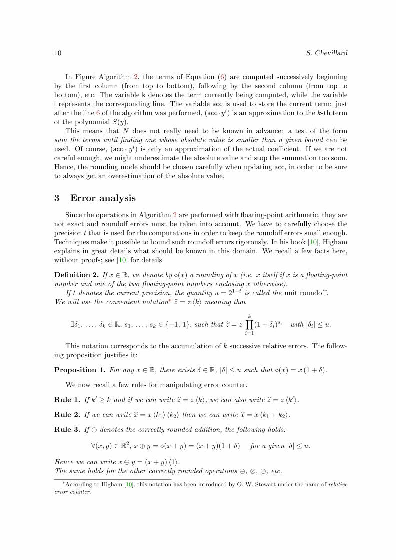
Let us do a complete analysis on a simple example. Consider a, b, c, d, e f six floating-point numbers. We want to compute S = a b + c d e + f . In practice, we may compute forinstance S = ((a⊗b)⊕((c⊗d)⊗e))⊕f . We can analyze the roundoff errors with the followingsimple arguments:
S =((a⊗ b) ⊕ ((c⊗ d)⊗ e)
)⊕ f
=((ab) 〈1〉 ⊕ (cde) 〈2〉
)⊕ f (Rule 3 applied to ⊗ and Rule 2)
=((ab) 〈2〉 ⊕ (cde) 〈2〉
)⊕ f (Rule 1)
=((ab) 〈2〉 + (cde) 〈2〉
)〈1〉 ⊕ f (Rule 3 applied to ⊕ )
=((ab) 〈3〉 + (cde) 〈3〉
)⊕ f (Rule 4 and Rule 2)
= (ab) 〈4〉 + (cde) 〈4〉 + f 〈4〉 (Rules 3, 4, 2 and 1).
We now need a proposition to bound the error corresponding to a given value of theerror counter:
Proposition 2. Let z ∈ R and let z be a floating-point number. We suppose that k ∈ N
satisfies ku < 1 and that we can write z = z 〈k〉. Then
∃θk ∈ R, such that z = z(1 + θk) with |θk| ≤ γk =ku
1− ku.
In particular, as soon as ku ≤ 1/2, γk ≤ 2ku.
Using this proposition, we can write S = (a b)(1 + θ4) + (c d e)(1 + θ′4) + f(1 + θ′′4). Finally,we get ∣∣∣S − S
∣∣∣ ≤ γ4 (|a b|+ |c d e|+ |f |) .
Note the importance of S = |a b|+ |c d e|+ |f |. If the terms of the sum are all non-negative,S = S and the relative error for the computation of the sum is bounded by γ4. If some termsare negative, the relative error is bounded by γ4S/S. The ratio S/S may be extremely large:this quantifies the phenomenon of cancellation, when terms of the sum cancel out while theerrors accumulate.
4 Practical implementation
4.1 General scheme
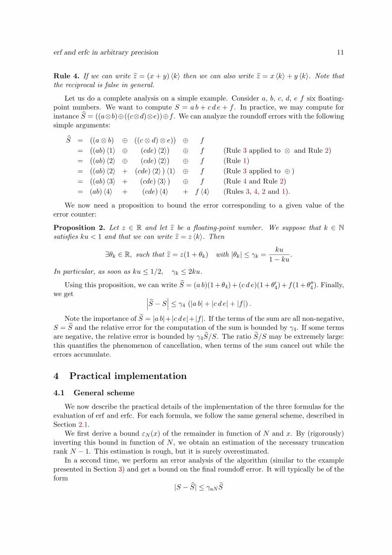
We now describe the practical details of the implementation of the three formulas for theevaluation of erf and erfc. For each formula, we follow the same general scheme, described inSection 2.1.
We first derive a bound εN (x) of the remainder in function of N and x. By (rigorously)inverting this bound in function of N , we obtain an estimation of the necessary truncationrank N − 1. This estimation is rough, but it is surely overestimated.
In a second time, we perform an error analysis of the algorithm (similar to the examplepresented in Section 3) and get a bound on the final roundoff error. It will typically be of theform
|S − S| ≤ γaN S
12 S. Chevillard
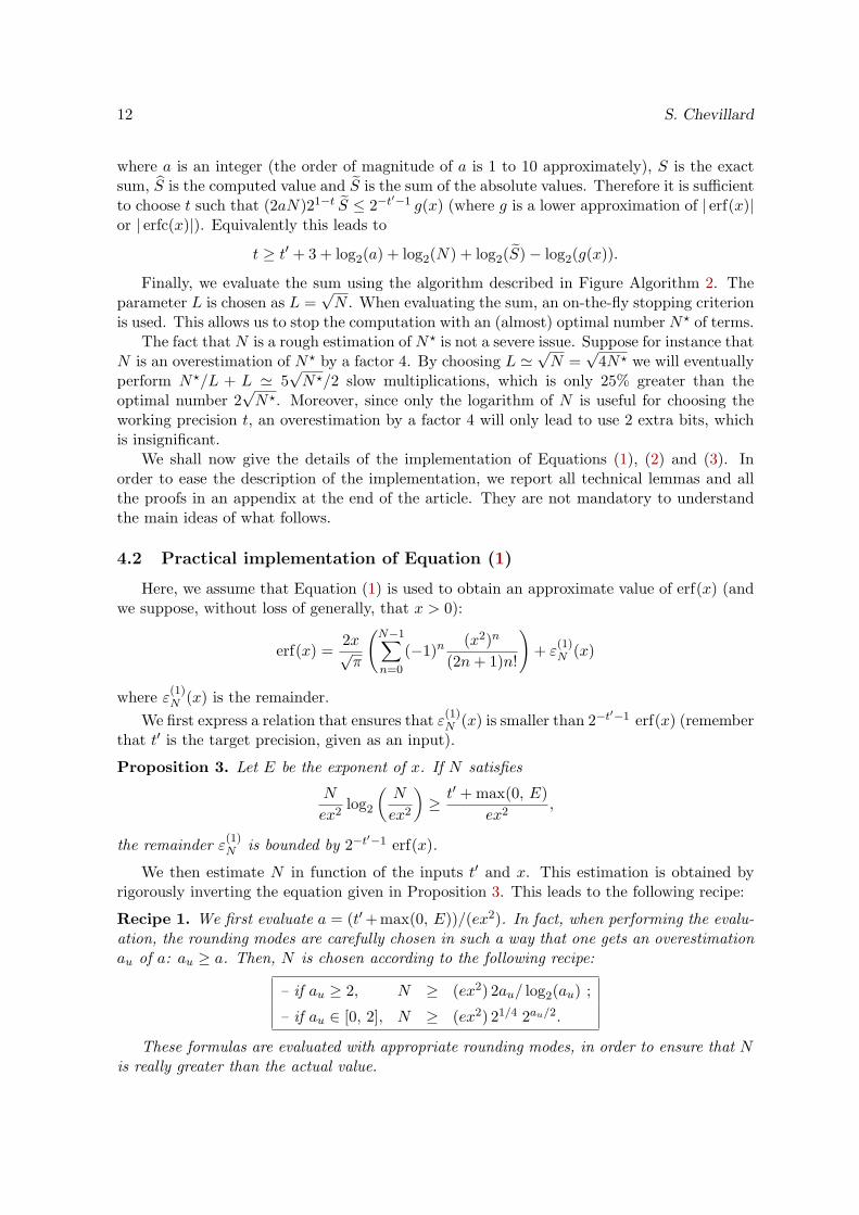
where a is an integer (the order of magnitude of a is 1 to 10 approximately), S is the exactsum, S is the computed value and S is the sum of the absolute values. Therefore it is sufficientto choose t such that (2aN)21−t S ≤ 2−t
′−1 g(x) (where g is a lower approximation of | erf(x)|or | erfc(x)|). Equivalently this leads to
t ≥ t′ + 3 + log2(a) + log2(N) + log2(S)− log2(g(x)).
Finally, we evaluate the sum using the algorithm described in Figure Algorithm 2. Theparameter L is chosen as L =
√N . When evaluating the sum, an on-the-fly stopping criterion
is used. This allows us to stop the computation with an (almost) optimal number N⋆ of terms.The fact that N is a rough estimation of N⋆ is not a severe issue. Suppose for instance that
N is an overestimation of N⋆ by a factor 4. By choosing L ≃√N =
√4N⋆ we will eventually
perform N⋆/L + L ≃ 5√N⋆/2 slow multiplications, which is only 25% greater than the
optimal number 2√N⋆. Moreover, since only the logarithm of N is useful for choosing the
working precision t, an overestimation by a factor 4 will only lead to use 2 extra bits, whichis insignificant.
We shall now give the details of the implementation of Equations (1), (2) and (3). Inorder to ease the description of the implementation, we report all technical lemmas and allthe proofs in an appendix at the end of the article. They are not mandatory to understandthe main ideas of what follows.
4.2 Practical implementation of Equation (1)
Here, we assume that Equation (1) is used to obtain an approximate value of erf(x) (andwe suppose, without loss of generally, that x > 0):
erf(x) =2x√π
(N−1∑
n=0
(−1)n(x2)n
(2n+ 1)n!
)+ ε
(1)N (x)
where ε(1)N (x) is the remainder.
We first express a relation that ensures that ε(1)N (x) is smaller than 2−t
′−1 erf(x) (rememberthat t′ is the target precision, given as an input).
Proposition 3. Let E be the exponent of x. If N satisfies
N
ex2log2
(N
ex2
)≥ t′ + max(0, E)
ex2,
the remainder ε(1)N is bounded by 2−t
′−1 erf(x).
We then estimate N in function of the inputs t′ and x. This estimation is obtained byrigorously inverting the equation given in Proposition 3. This leads to the following recipe:
Recipe 1. We first evaluate a = (t′+ max(0, E))/(ex2). In fact, when performing the evalu-ation, the rounding modes are carefully chosen in such a way that one gets an overestimationau of a: au ≥ a. Then, N is chosen according to the following recipe:
– if au ≥ 2, N ≥ (ex2) 2au/ log2(au) ;
– if au ∈ [0, 2], N ≥ (ex2) 21/4 2au/2.
These formulas are evaluated with appropriate rounding modes, in order to ensure that Nis really greater than the actual value.
erf and erfc in arbitrary precision 13
Once an overestimation N − 1 of the truncation rank is known, we need to choose aworking precision t. This precision depends on the errors that will be accumulated during theevaluation. So, we first sketch the details of the evaluation.
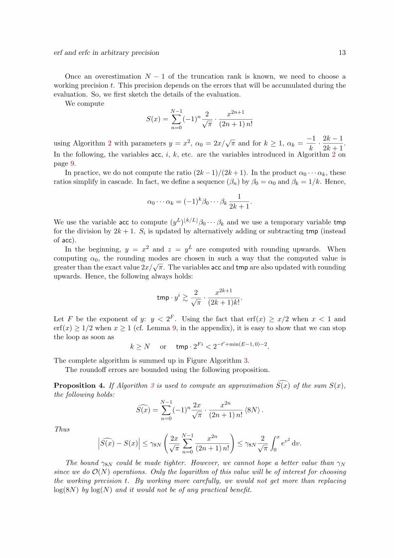
We compute
S(x) =N−1∑
n=0
(−1)n2√π· x2n+1
(2n+ 1)n!
using Algorithm 2 with parameters y = x2, α0 = 2x/√π and for k ≥ 1, αk =
−1
k· 2k − 1
2k + 1.
In the following, the variables acc, i, k, etc. are the variables introduced in Algorithm 2 onpage 9.
In practice, we do not compute the ratio (2k−1)/(2k+ 1). In the product α0 · · ·αk, theseratios simplify in cascade. In fact, we define a sequence (βn) by β0 = α0 and βk = 1/k. Hence,
α0 · · ·αk = (−1)kβ0 · · ·βk1
2k + 1.
We use the variable acc to compute (yL)⌊k/L⌋β0 · · ·βk and we use a temporary variable tmp
for the division by 2k + 1. Si is updated by alternatively adding or subtracting tmp (insteadof acc).
In the beginning, y = x2 and z = yL are computed with rounding upwards. Whencomputing α0, the rounding modes are chosen in such a way that the computed value isgreater than the exact value 2x/
√π. The variables acc and tmp are also updated with rounding
upwards. Hence, the following always holds:
tmp · yi & 2√π· x
2k+1
(2k + 1)k!.
Let F be the exponent of y: y < 2F . Using the fact that erf(x) ≥ x/2 when x < 1 anderf(x) ≥ 1/2 when x ≥ 1 (cf. Lemma 9, in the appendix), it is easy to show that we can stopthe loop as soon as
k ≥ N or tmp · 2Fi < 2−t′+min(E−1, 0)−2.
The complete algorithm is summed up in Figure Algorithm 3.
The roundoff errors are bounded using the following proposition.
Proposition 4. If Algorithm 3 is used to compute an approximation S(x) of the sum S(x),the following holds:
S(x) =N−1∑
n=0
(−1)n2x√π· x2n
(2n+ 1)n!〈8N〉 .
Thus∣∣∣S(x)− S(x)
∣∣∣ ≤ γ8N(
2x√π
N−1∑
n=0
x2n
(2n+ 1)n!
)≤ γ8N
2√π
∫ x
0ev
2
dv.
The bound γ8N could be made tighter. However, we cannot hope a better value than γNsince we do O(N) operations. Only the logarithm of this value will be of interest for choosingthe working precision t. By working more carefully, we would not get more than replacinglog(8N) by log(N) and it would not be of any practical benefit.
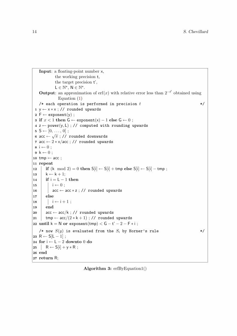
14 S. Chevillard
Input: a floating-point number x,the working precision t,the target precision t’,L ∈ N⋆, N ∈ N⋆.
Output: an approximation of erf(x) with relative error less than 2−t′
obtained usingEquation (1)
/* each operation is performed in precision t */
y← x ∗ x ; // rounded upwards1
F← exponent(y) ;2
if x < 1 then G← exponent(x)− 1 else G← 0 ;3
z← power(y, L) ; // computed with rounding upwards4
S← [0, . . . , 0] ;5
acc← √π ; // rounded downwards6
acc← 2 ∗ x/acc ; // rounded upwards7
i← 0 ;8
k← 0 ;9
tmp← acc ;10
repeat11
if (k mod 2) = 0 then S[i]← S[i] + tmp else S[i]← S[i]− tmp ;12
k← k + 1;13
if i = L− 1 then14
i← 0 ;15
acc← acc ∗ z ; // rounded upwards16
else17
i← i + 1 ;18
end19
acc← acc/k ; // rounded upwards20
tmp← acc/(2 ∗ k + 1) ; // rounded upwards21
until k = N or exponent(tmp) < G− t’− 2− F ∗ i ;22
/* now S(y) is evaluated from the Si by Horner’s rule */
R← S[L− 1] ;23
for i← L− 2 downto 0 do24
R← S[i] + y ∗ R ;25
end26
return R;27
Algorithm 3: erfByEquation1()
erf and erfc in arbitrary precision 15
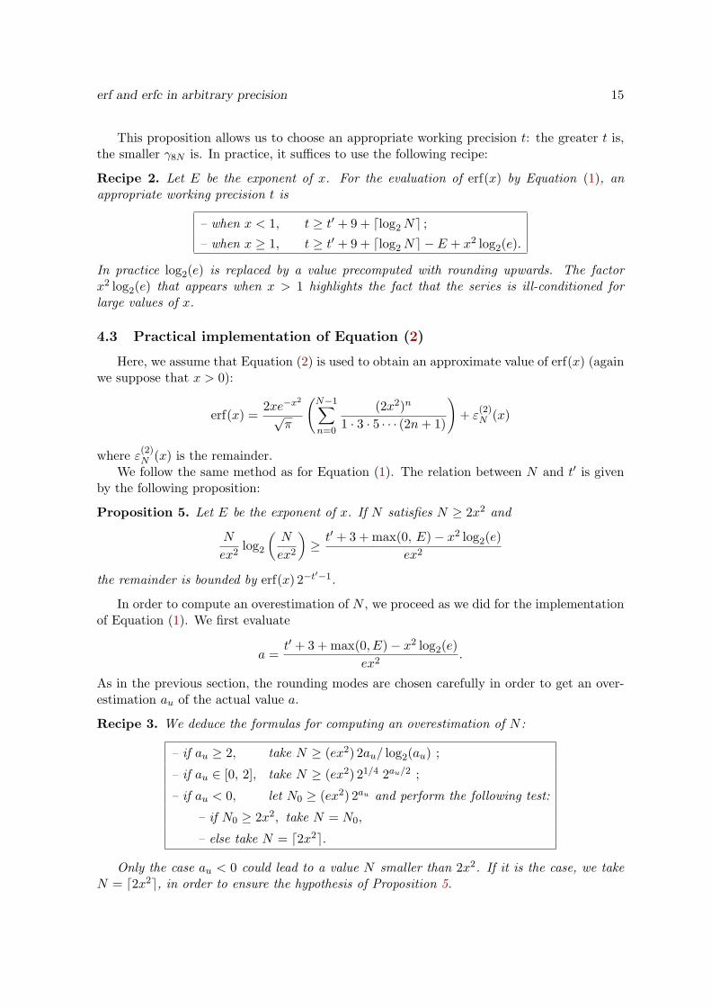
This proposition allows us to choose an appropriate working precision t: the greater t is,the smaller γ8N is. In practice, it suffices to use the following recipe:
Recipe 2. Let E be the exponent of x. For the evaluation of erf(x) by Equation (1), anappropriate working precision t is
– when x < 1, t ≥ t′ + 9 + ⌈log2N⌉ ;
– when x ≥ 1, t ≥ t′ + 9 + ⌈log2N⌉ − E + x2 log2(e).
In practice log2(e) is replaced by a value precomputed with rounding upwards. The factorx2 log2(e) that appears when x > 1 highlights the fact that the series is ill-conditioned forlarge values of x.
4.3 Practical implementation of Equation (2)
Here, we assume that Equation (2) is used to obtain an approximate value of erf(x) (againwe suppose that x > 0):
erf(x) =2xe−x
2
√π
(N−1∑
n=0
(2x2)n
1 · 3 · 5 · · · (2n+ 1)
)+ ε
(2)N (x)
where ε(2)N (x) is the remainder.
We follow the same method as for Equation (1). The relation between N and t′ is givenby the following proposition:
Proposition 5. Let E be the exponent of x. If N satisfies N ≥ 2x2 and
N
ex2log2
(N
ex2
)≥ t′ + 3 + max(0, E)− x2 log2(e)
ex2
the remainder is bounded by erf(x) 2−t′−1.
In order to compute an overestimation of N , we proceed as we did for the implementationof Equation (1). We first evaluate
a =t′ + 3 + max(0, E)− x2 log2(e)
ex2.
As in the previous section, the rounding modes are chosen carefully in order to get an over-estimation au of the actual value a.
Recipe 3. We deduce the formulas for computing an overestimation of N :
– if au ≥ 2, take N ≥ (ex2) 2au/ log2(au) ;
– if au ∈ [0, 2], take N ≥ (ex2) 21/4 2au/2 ;
– if au < 0, let N0 ≥ (ex2) 2au and perform the following test:
– if N0 ≥ 2x2, take N = N0,
– else take N = ⌈2x2⌉.
Only the case au < 0 could lead to a value N smaller than 2x2. If it is the case, we takeN = ⌈2x2⌉, in order to ensure the hypothesis of Proposition 5.
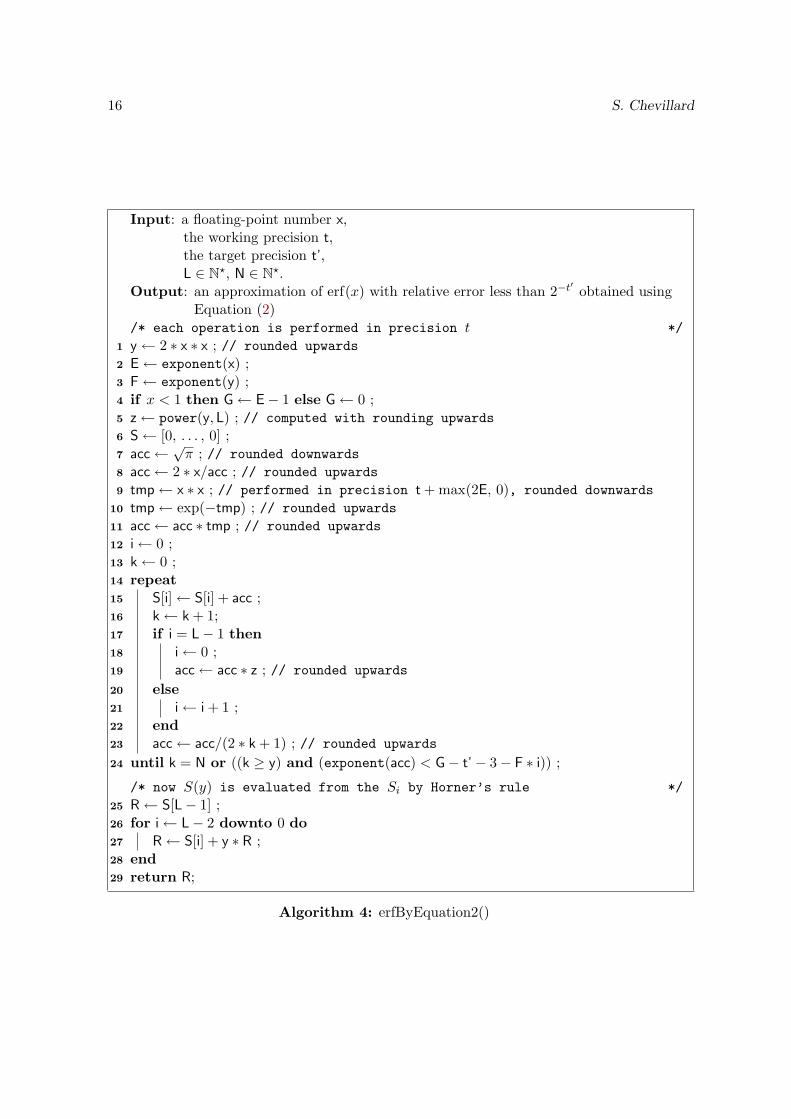
16 S. Chevillard
Input: a floating-point number x,the working precision t,the target precision t’,L ∈ N⋆, N ∈ N⋆.
Output: an approximation of erf(x) with relative error less than 2−t′
obtained usingEquation (2)
/* each operation is performed in precision t */
y← 2 ∗ x ∗ x ; // rounded upwards1
E← exponent(x) ;2
F← exponent(y) ;3
if x < 1 then G← E− 1 else G← 0 ;4
z← power(y, L) ; // computed with rounding upwards5
S← [0, . . . , 0] ;6
acc← √π ; // rounded downwards7
acc← 2 ∗ x/acc ; // rounded upwards8
tmp← x ∗ x ; // performed in precision t + max(2E, 0), rounded downwards9
tmp← exp(−tmp) ; // rounded upwards10
acc← acc ∗ tmp ; // rounded upwards11
i← 0 ;12
k← 0 ;13
repeat14
S[i]← S[i] + acc ;15
k← k + 1;16
if i = L− 1 then17
i← 0 ;18
acc← acc ∗ z ; // rounded upwards19
else20
i← i + 1 ;21
end22
acc← acc/(2 ∗ k + 1) ; // rounded upwards23
until k = N or ((k ≥ y) and (exponent(acc) < G− t’− 3− F ∗ i)) ;24
/* now S(y) is evaluated from the Si by Horner’s rule */
R← S[L− 1] ;25
for i← L− 2 downto 0 do26
R← S[i] + y ∗ R ;27
end28
return R;29
Algorithm 4: erfByEquation2()
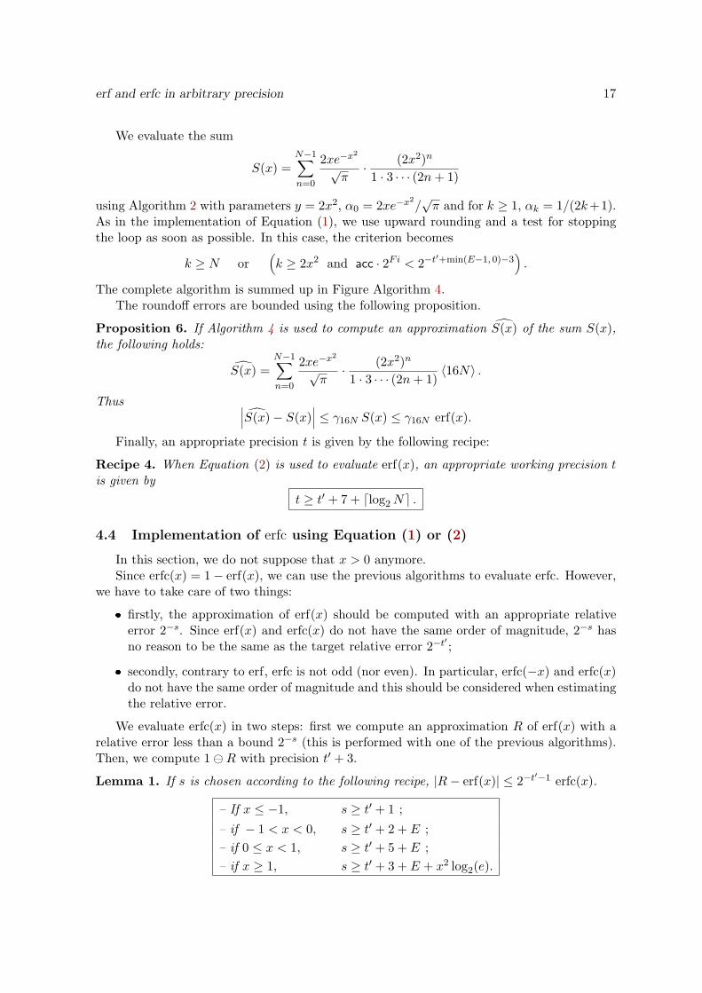
erf and erfc in arbitrary precision 17
We evaluate the sum
S(x) =N−1∑
n=0
2xe−x2
√π· (2x2)n
1 · 3 · · · (2n+ 1)
using Algorithm 2 with parameters y = 2x2, α0 = 2xe−x2
/√π and for k ≥ 1, αk = 1/(2k+1).
As in the implementation of Equation (1), we use upward rounding and a test for stoppingthe loop as soon as possible. In this case, the criterion becomes
k ≥ N or(k ≥ 2x2 and acc · 2Fi < 2−t
′+min(E−1, 0)−3).
The complete algorithm is summed up in Figure Algorithm 4.The roundoff errors are bounded using the following proposition.
Proposition 6. If Algorithm 4 is used to compute an approximation S(x) of the sum S(x),the following holds:
S(x) =N−1∑
n=0
2xe−x2
√π· (2x2)n
1 · 3 · · · (2n+ 1)〈16N〉 .
Thus ∣∣∣S(x)− S(x)∣∣∣ ≤ γ16N S(x) ≤ γ16N erf(x).
Finally, an appropriate precision t is given by the following recipe:
Recipe 4. When Equation (2) is used to evaluate erf(x), an appropriate working precision tis given by
t ≥ t′ + 7 + ⌈log2N⌉ .
4.4 Implementation of erfc using Equation (1) or (2)
In this section, we do not suppose that x > 0 anymore.Since erfc(x) = 1− erf(x), we can use the previous algorithms to evaluate erfc. However,
we have to take care of two things:
❼ firstly, the approximation of erf(x) should be computed with an appropriate relativeerror 2−s. Since erf(x) and erfc(x) do not have the same order of magnitude, 2−s hasno reason to be the same as the target relative error 2−t
′
;
❼ secondly, contrary to erf, erfc is not odd (nor even). In particular, erfc(−x) and erfc(x)do not have the same order of magnitude and this should be considered when estimatingthe relative error.
We evaluate erfc(x) in two steps: first we compute an approximation R of erf(x) with arelative error less than a bound 2−s (this is performed with one of the previous algorithms).Then, we compute 1⊖R with precision t′ + 3.
Lemma 1. If s is chosen according to the following recipe, |R− erf(x)| ≤ 2−t′−1 erfc(x).
– If x ≤ −1, s ≥ t′ + 1 ;
– if − 1 < x < 0, s ≥ t′ + 2 + E ;
– if 0 ≤ x < 1, s ≥ t′ + 5 + E ;
– if x ≥ 1, s ≥ t′ + 3 + E + x2 log2(e).
18 S. Chevillard
As a consequence of the lemma,
|(1−R)− erfc(x)| ≤ 2−t′−1 erfc(x).
It follows that |(1−R)| ≤ 2 erfc(x). Now, since (1⊖R) = (1−R) 〈1〉,∣∣(1⊖R)− (1−R)
∣∣ ≤ |(1−R)| 21−(t′+3) ≤ 2−t′−1 erfc(x).
Finally∣∣(1 ⊖ R) − erfc(x)
∣∣ ≤∣∣(1 ⊖ R) − (1 − R)
∣∣ +∣∣(1 − R) − erfc(x)
∣∣ ≤ 2−t′
erfc(x) which
proves that (1⊖R) is an approximation of erfc(x) with a relative error bounded by 2−t′
.Important remark: in the case when −1 < x < 0 and when t′ + 2 + E ≤ 1, it is actuallynot necessary to perform any computation: in this case, 1 is an approximation to erfc(x) witha relative error less than 2−t
′
. More precisely, we have |x| ≤ 2E ≤ 2−t′−1, so
|1− erfc(x)| = | erf(x)| = | erf(|x|)|.
We can bound | erf(|x|)| by 2x (see Lemma 9 in Appendix). Moreover, since x < 0, erfc(x) > 1.So we have |1− erfc(x)| ≤ 2−t
′
erfc(x).The same remark holds in the case when 0 < x < 1 and t′ + 5 + E ≤ 1.
4.5 Practical implementation of Equation (3)
We now show how to use Equation (3) for obtaining an approximate value of erfc(x) (wesuppose again that x > 0):
erfc(x) =e−x
2
x√π
(1 +
N−1∑
n=1
(−1)n1 · 3 · 5 · · · (2n− 1)
(2x2)n
)+ ε
(3)N (x)
where ε(3)N (x) is the remainder, bounded thanks to Inequality (4).
The particularity of this formula comes from the fact that the remainder cannot be madearbitrarily small. In fact, x being given, the bound (4) is first decreasing until it reaches anoptimal value with N = ⌊x2 + 1/2⌋. For larger values of N , it increases. Hence, given atarget relative error 2−t
′
, it may be possible that no value of N is satisfying. In this case,Equation (3) cannot be used. We note in particular that this formula is useless for 0 < x < 1.Until the end of this section, we will suppose that x ≥ 1.
Conversely, when the relative error can be achieved, we can choose any value of N betweentwo values Nmin and Nmax. Obviously, we are interested in the smallest one.
Proposition 7. If N satisfies
N
ex2log2
(N
ex2
)≤ −t
′ − 3
ex2
the remainder is bounded by erfc(x) 2−t′−1.
Using this proposition, it is possible to compute an overestimation N of Nmin. However,it is possible that this estimation N could be even greater than Nmax. In order to avoidthis possibility, let us remark two things: firstly, we never need to consider values N greaterthan x2 (since we know the bound given by Equation (4) is minimal for N = ⌊x2 − 1/2⌋)and, secondly, given a candidate value N , it is always possible to check if the inequality ofProposition (7) holds.
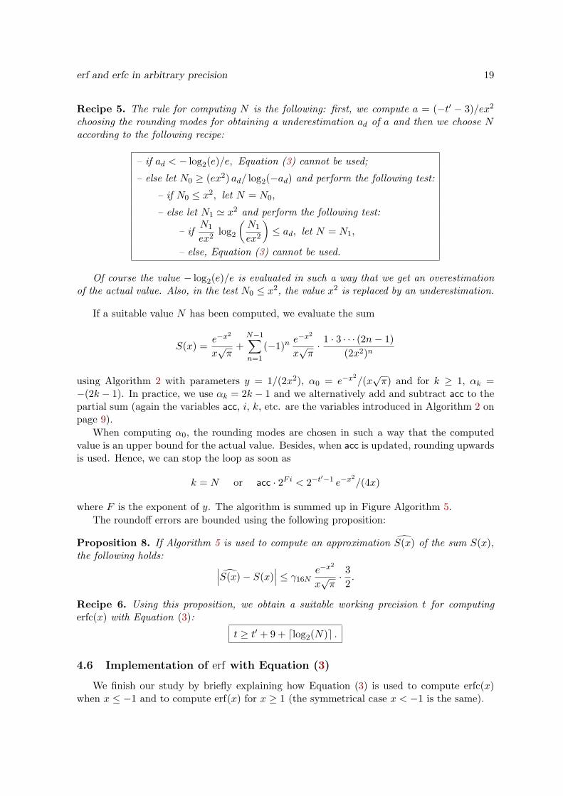
erf and erfc in arbitrary precision 19
Recipe 5. The rule for computing N is the following: first, we compute a = (−t′ − 3)/ex2
choosing the rounding modes for obtaining a underestimation ad of a and then we choose Naccording to the following recipe:
– if ad < − log2(e)/e, Equation (3) cannot be used;
– else let N0 ≥ (ex2) ad/ log2(−ad) and perform the following test:
– if N0 ≤ x2, let N = N0,
– else let N1 ≃ x2 and perform the following test:
– ifN1
ex2log2
(N1
ex2
)≤ ad, let N = N1,
– else, Equation (3) cannot be used.
Of course the value − log2(e)/e is evaluated in such a way that we get an overestimationof the actual value. Also, in the test N0 ≤ x2, the value x2 is replaced by an underestimation.
If a suitable value N has been computed, we evaluate the sum
S(x) =e−x
2
x√π
+N−1∑
n=1
(−1)ne−x
2
x√π· 1 · 3 · · · (2n− 1)
(2x2)n
using Algorithm 2 with parameters y = 1/(2x2), α0 = e−x2
/(x√π) and for k ≥ 1, αk =
−(2k − 1). In practice, we use αk = 2k − 1 and we alternatively add and subtract acc to thepartial sum (again the variables acc, i, k, etc. are the variables introduced in Algorithm 2 onpage 9).
When computing α0, the rounding modes are chosen in such a way that the computedvalue is an upper bound for the actual value. Besides, when acc is updated, rounding upwardsis used. Hence, we can stop the loop as soon as
k = N or acc · 2Fi < 2−t′−1 e−x
2
/(4x)
where F is the exponent of y. The algorithm is summed up in Figure Algorithm 5.
The roundoff errors are bounded using the following proposition:
Proposition 8. If Algorithm 5 is used to compute an approximation S(x) of the sum S(x),the following holds:
∣∣∣S(x)− S(x)∣∣∣ ≤ γ16N
e−x2
x√π· 3
2.
Recipe 6. Using this proposition, we obtain a suitable working precision t for computingerfc(x) with Equation (3):
t ≥ t′ + 9 + ⌈log2(N)⌉ .
4.6 Implementation of erf with Equation (3)
We finish our study by briefly explaining how Equation (3) is used to compute erfc(x)when x ≤ −1 and to compute erf(x) for x ≥ 1 (the symmetrical case x < −1 is the same).
20 S. Chevillard
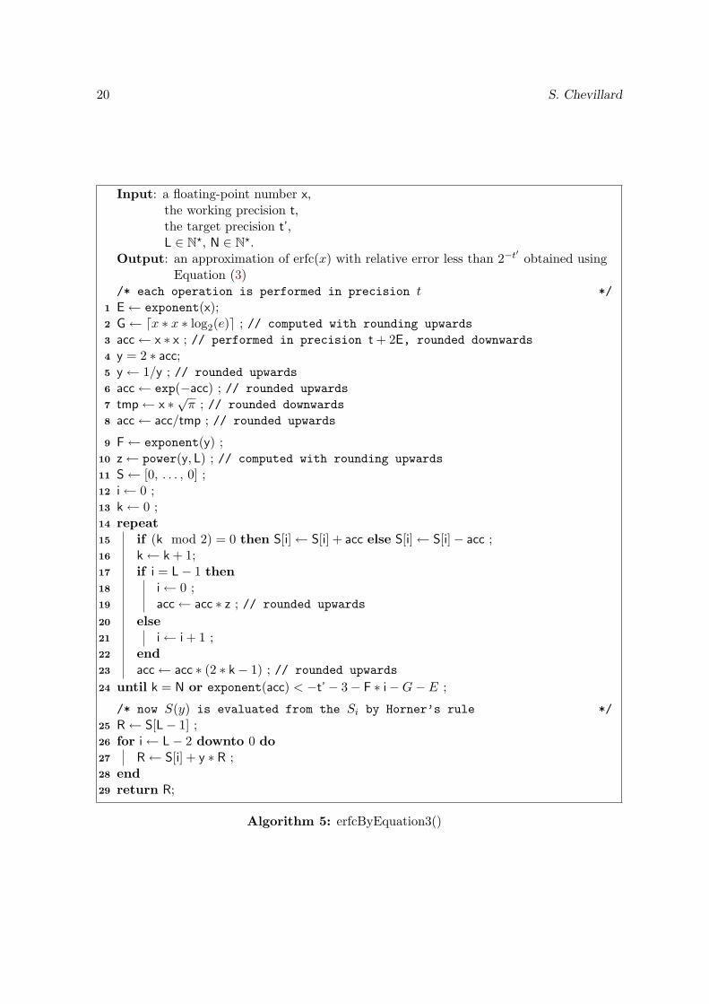
Input: a floating-point number x,the working precision t,the target precision t’,L ∈ N⋆, N ∈ N⋆.
Output: an approximation of erfc(x) with relative error less than 2−t′
obtained usingEquation (3)
/* each operation is performed in precision t */
E← exponent(x);1
G← ⌈x ∗ x ∗ log2(e)⌉ ; // computed with rounding upwards2
acc← x ∗ x ; // performed in precision t + 2E, rounded downwards3
y = 2 ∗ acc;4
y← 1/y ; // rounded upwards5
acc← exp(−acc) ; // rounded upwards6
tmp← x ∗ √π ; // rounded downwards7
acc← acc/tmp ; // rounded upwards8
F← exponent(y) ;9
z← power(y, L) ; // computed with rounding upwards10
S← [0, . . . , 0] ;11
i← 0 ;12
k← 0 ;13
repeat14
if (k mod 2) = 0 then S[i]← S[i] + acc else S[i]← S[i]− acc ;15
k← k + 1;16
if i = L− 1 then17
i← 0 ;18
acc← acc ∗ z ; // rounded upwards19
else20
i← i + 1 ;21
end22
acc← acc ∗ (2 ∗ k− 1) ; // rounded upwards23
until k = N or exponent(acc) < −t’− 3− F ∗ i−G− E ;24
/* now S(y) is evaluated from the Si by Horner’s rule */
R← S[L− 1] ;25
for i← L− 2 downto 0 do26
R← S[i] + y ∗ R ;27
end28
return R;29
Algorithm 5: erfcByEquation3()
erf and erfc in arbitrary precision 21
Note that erfc(x) = 1 − erf(x) = 1 + erf(−x) = 2 − erfc(−x). When x ≤ −1, we obtainerfc(x) by computing an approximation R of erfc(−x) with a relative error smaller than anappropriate bound 2−s and computing 2⊖R in precision t′ + 3.
The same way, since erf(x) = 1−erfc(x), we obtain erf(x) by computing an approximationR of erfc(x) with a relative error smaller than an appropriate bound 2−s and computing 1⊖Rin precision t′ + 3.
The appropriate values for s are given in the two following lemmas.
Lemma 2. If x ≥ 1, the inequality |R− erfc(x)| ≤ 2−t′−1 erfc(−x) holds when s is chosen
according to the following recipe:
s ≥ t′ + 2− E − x2 log2(e).
Remark that whenever t′ + 2 − E − x2 log2(e) ≤ 1, it is not necessary to compute anapproximation of erfc(x) and to perform the subtraction: 2 can be directly returned as aresult. Indeed, t′ + 2− E − x2 log2(e) ≤ 1 implies that e−x
2
/x ≤ 2−t′
and hence
erfc(x) ≤ 2−t′ ≤ 2−t
′
erfc(−x).
Since erfc(x) = 2− erfc(−x), it means that 2 is an approximation of erfc(−x) with a relativeerror less than 2−t
′
.
Lemma 3. If x ≥ 1 the inequality |R− erfc(x)| ≤ 2−t′−1 erf(x) holds when s is chosen
according to the following recipe:
s ≥ t′ + 3− E − x2 log2(e).
The same remark holds: if t′+ 3−E−x2 log2(e) ≤ 1, the value 1 can be directly returnedas an approximation of erf(x) with a relative error less than 2−t
′
.
5 Experimental results
We have given all the details necessary for implementing each of the three equations (1), (2),and (3). They can be used for obtaining approximate values of either erf(x) or erfc(x). Wealso gave estimations of the order of truncation N − 1 and of the working precision t. In eachcase O(
√N) multiplications at precision t and O(N) additions and multiplications/divisions
by small integers are needed for evaluating the sum. Hence, for each equation, the binarycomplexity of the algorithm is O(
√N M(t) +Nt) where M(t) denotes the binary complexity
of a product of two numbers of precision t.However, quite different behaviors are hidden behind this complexity. Indeed, the inputs
of our algorithms are the point x and the target precision t′. Hence, N and t are functions ofx and t′. As can be seen in previous sections, these functions highly depend on the equationused to evaluate erf(x) or erfc(x).
5.1 Choosing the best equation
Of course, given an input couple (x, t′), we would like to automatically choose the equationto be used, in order to minimize the computation time. For this purpose, we need to comparethe complexity of the three equations. It seems quite hard to theoretically perform such acomparison:
22 S. Chevillard
❼ firstly, the estimations of N and t are different for each equation. They depend on xand t′ in a complicated way. Besides, they are defined piecewise, which implies thatthere are many cases to study;
❼ secondly, comparing the three methods requires to set some assumptions on the imple-mentation of the underlying arithmetic (e.g. complexity of the multiplication; complex-ity of the evaluation of exp).
Usually, the multiplication between two numbers of precision t is performed differentlywhether t is large or not: see [9, Section 2.4] for an overview of what is used in MPFR.Three different algorithms are used in MPFR, and each one depends on the underlying integermultiplication. The GMP library, used to perform the integer multiplications, uses at least fourdifferent algorithms depending on the sizes of the input data. Hence, the effective complexityM(t) is very hard to accurately estimate.
In MPFR, the evaluation of exp(x) is performed by three different algorithms, dependingon the required precision t (see [9, end of Section 2.5] for a brief overview).
❼ A naive evaluation of the series is used when t is smaller than a parameter t0;
❼ the concurrent series technique of Smith is used when t lies between t0 and a secondthreshold t1;
❼ finally, if t ≥ t1, a binary splitting method [3] is used.
The values t0 and t1 have been tuned (and are thus different) for each architecture.This shows that choosing the best equation between the three equations proposed in
this paper is a matter of practice and not of theoretical study. We implemented the threealgorithms in C, using MPFR for the floating-point arithmetic. Our code is distributed underthe LGPL and freely available at http://prunel.ccsd.cnrs.fr/ensl-00356709/.
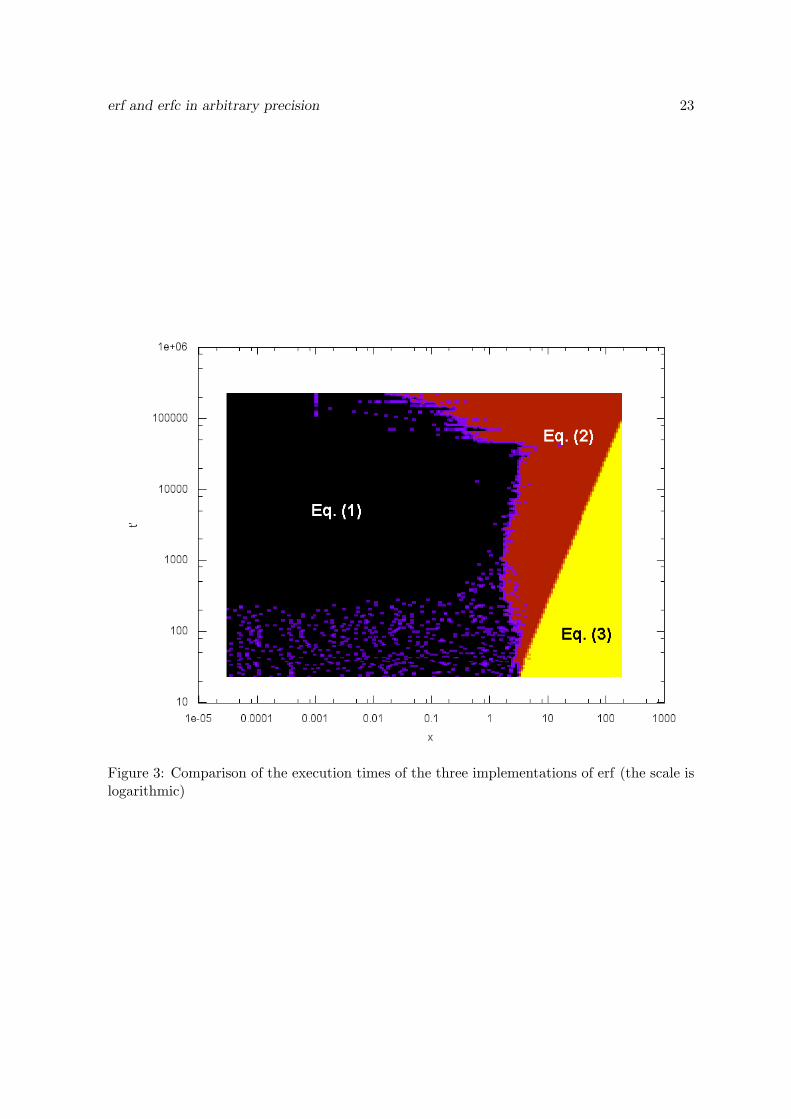
In order to experimentally see which equation is the best for each couple (x, t′), we ranthe three implementations for a large range of values x and t′. For each couple, we comparedthe execution time of each implementation when evaluating erf(x). The experimental resultsare summed up in Figure 3. The colors indicate which implementation is the fastest. Theexperiments were performed on a 32-bit 3.00 GHz Intel Pentium D with 2.00 GB of RAMrunning Linux 2.6.26 and MPFR 2.3.1 and gcc 4.3.3. The thresholds used by MPFR for thisarchitecture are t0 = 528 and t1 = 47 120.
The boundary between Equations (1) and (2) seems to exhibit three phases, dependingon t′. These phases approximately match the thresholds used by MPFR for the implementationof exp. Since Equation (2) relies on the evaluation of exp(−x2) whereas Equation (1) does not,this is probably not a coincidence and we just see the impact of the evaluation of exp(−x2)on the whole computation time.
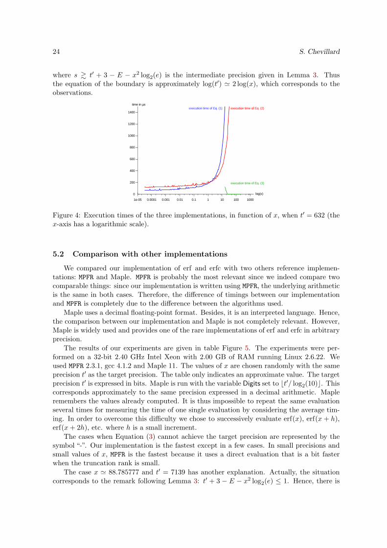
The boundary between Equations (2) and (3) is more regular. In fact, we experimentallyobserve that as soon as Equation (3) is usable, it is more interesting than the other equations.Figure 4 shows the timings for t′ = 632 in function of x. This is a typical situation: for smallvalues of x, Equation (3) cannot achieve the target precision; but for x ≃ 15, it becomes usableand is immediately five times faster than the others. Hence, the domain where Equation (3)should be used is given by the points where the inequality of Proposition 7 has a solution, i.e.if and only if
−s− 3
ex2≥ − log2(e)
e,
erf and erfc in arbitrary precision 23
Figure 3: Comparison of the execution times of the three implementations of erf (the scale islogarithmic)
24 S. Chevillard
where s & t′ + 3 − E − x2 log2(e) is the intermediate precision given in Lemma 3. Thusthe equation of the boundary is approximately log(t′) ≃ 2 log(x), which corresponds to theobservations.
Figure 4: Execution times of the three implementations, in function of x, when t′ = 632 (thex-axis has a logarithmic scale).
5.2 Comparison with other implementations
We compared our implementation of erf and erfc with two others reference implemen-tations: MPFR and Maple. MPFR is probably the most relevant since we indeed compare twocomparable things: since our implementation is written using MPFR, the underlying arithmeticis the same in both cases. Therefore, the difference of timings between our implementationand MPFR is completely due to the difference between the algorithms used.
Maple uses a decimal floating-point format. Besides, it is an interpreted language. Hence,the comparison between our implementation and Maple is not completely relevant. However,Maple is widely used and provides one of the rare implementations of erf and erfc in arbitraryprecision.
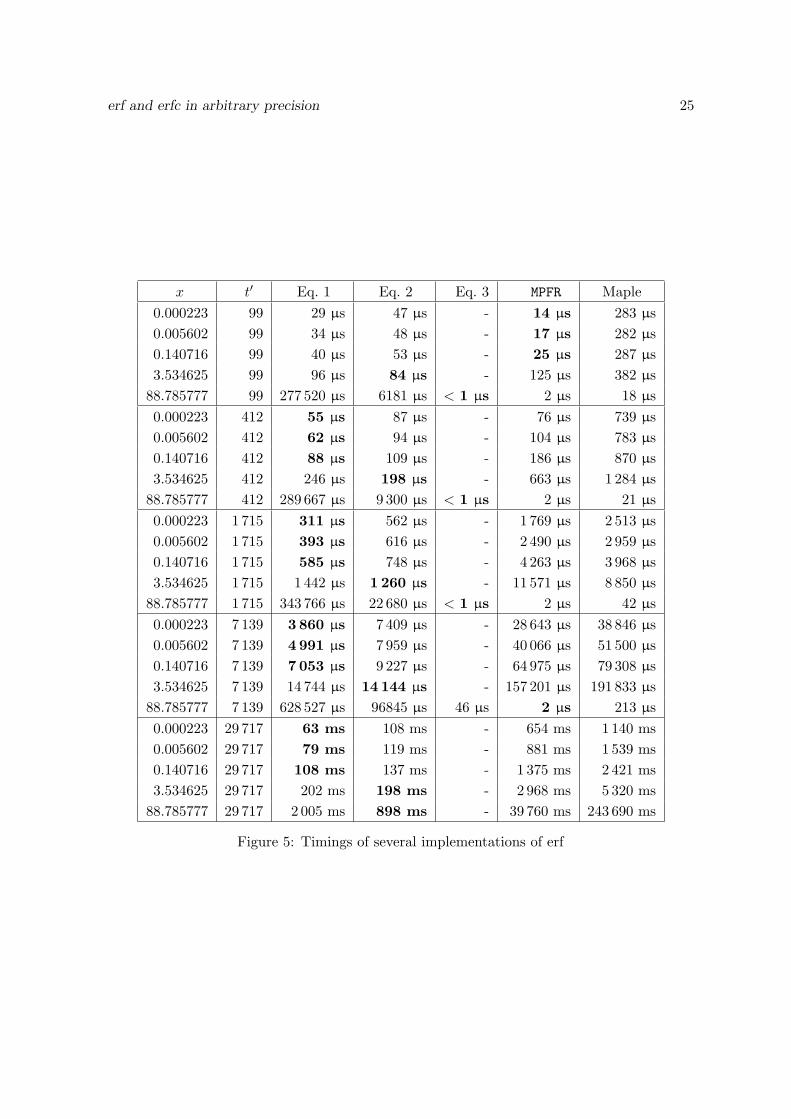
The results of our experiments are given in table Figure 5. The experiments were per-formed on a 32-bit 2.40 GHz Intel Xeon with 2.00 GB of RAM running Linux 2.6.22. Weused MPFR 2.3.1, gcc 4.1.2 and Maple 11. The values of x are chosen randomly with the sameprecision t′ as the target precision. The table only indicates an approximate value. The targetprecision t′ is expressed in bits. Maple is run with the variable Digits set to ⌊t′/ log2(10)⌋. Thiscorresponds approximately to the same precision expressed in a decimal arithmetic. Mapleremembers the values already computed. It is thus impossible to repeat the same evaluationseveral times for measuring the time of one single evaluation by considering the average tim-ing. In order to overcome this difficulty we chose to successively evaluate erf(x), erf(x + h),erf(x+ 2h), etc. where h is a small increment.
The cases when Equation (3) cannot achieve the target precision are represented by thesymbol “-”. Our implementation is the fastest except in a few cases. In small precisions andsmall values of x, MPFR is the fastest because it uses a direct evaluation that is a bit fasterwhen the truncation rank is small.
The case x ≃ 88.785777 and t′ = 7139 has another explanation. Actually, the situationcorresponds to the remark following Lemma 3: t′ + 3 − E − x2 log2(e) ≤ 1. Hence, there is
erf and erfc in arbitrary precision 25
x t′ Eq. 1 Eq. 2 Eq. 3 MPFR Maple
0.000223 99 29 µs 47 µs - 14 µs 283 µs
0.005602 99 34 µs 48 µs - 17 µs 282 µs
0.140716 99 40 µs 53 µs - 25 µs 287 µs
3.534625 99 96 µs 84 µs - 125 µs 382 µs
88.785777 99 277 520 µs 6181 µs < 1 µs 2 µs 18 µs
0.000223 412 55 µs 87 µs - 76 µs 739 µs
0.005602 412 62 µs 94 µs - 104 µs 783 µs
0.140716 412 88 µs 109 µs - 186 µs 870 µs
3.534625 412 246 µs 198 µs - 663 µs 1 284 µs
88.785777 412 289 667 µs 9 300 µs < 1 µs 2 µs 21 µs
0.000223 1 715 311 µs 562 µs - 1 769 µs 2 513 µs
0.005602 1 715 393 µs 616 µs - 2 490 µs 2 959 µs
0.140716 1 715 585 µs 748 µs - 4 263 µs 3 968 µs
3.534625 1 715 1 442 µs 1 260 µs - 11 571 µs 8 850 µs
88.785777 1 715 343 766 µs 22 680 µs < 1 µs 2 µs 42 µs
0.000223 7 139 3 860 µs 7 409 µs - 28 643 µs 38 846 µs
0.005602 7 139 4 991 µs 7 959 µs - 40 066 µs 51 500 µs
0.140716 7 139 7 053 µs 9 227 µs - 64 975 µs 79 308 µs
3.534625 7 139 14 744 µs 14 144 µs - 157 201 µs 191 833 µs
88.785777 7 139 628 527 µs 96845 µs 46 µs 2 µs 213 µs
0.000223 29 717 63 ms 108 ms - 654 ms 1 140 ms
0.005602 29 717 79 ms 119 ms - 881 ms 1 539 ms
0.140716 29 717 108 ms 137 ms - 1 375 ms 2 421 ms
3.534625 29 717 202 ms 198 ms - 2 968 ms 5 320 ms
88.785777 29 717 2 005 ms 898 ms - 39 760 ms 243 690 ms
Figure 5: Timings of several implementations of erf
26 S. Chevillard
nothing to compute and 1 can be returned immediately. In our implementation t′ + 3−E −x2 log2(e) is computed using MPFR in small precision. This takes 46 µs. MPFR performs thesame kind of test but using hardware arithmetic. This explains that it can give an answerin 2 µs.
6 Conclusion and perspectives
We proposed three algorithms for efficiently evaluating the functions erf and erfc in ar-bitrary precision. These algorithms are based on three different summation formulas whosecoefficients have the same general recursive structure. For evaluating the sum, we take advan-tage of this structure by using an algorithm due to Smith that makes it possible to evaluatethe sum with the binary complexity O(Nt + M(t)
√N) (this should be compared to the
complexity O(N M(t)) of the straightforward evaluation algorithm).
We gave closed formulas for upper-bounding the truncation rank N−1 and we completelystudied the effects of roundoff errors in the summation. We derived from this study closedformulas for the required working precision.
An interesting feature of our work comes from the fact that the errors are rigorouslybounded (and not only roughly estimated): to our best knowledge, the MPFR library is the onlyother library providing implementations with such guaranteed bounds. However, there was nocomplete documentation explaining how to write such an implementation. The general schemeexposed in this article can be used for the implementation of other functions: we completelydetailed the proofs and the algorithms in order to allow one to reproduce the same steps whenimplementing other functions. Examples of functions that could be implemented using thisscheme include Fresnel integrals, Exponential integrals or Airy functions when x ≥ 0. Thescheme would require slight modifications for other functions such as Airy functions whenx < 0 or Bessel functions because these functions have several zeros. Due to these zeros, itis not possible to find an underestimation g (as required in our general scheme in page 4).Nevertheless, even for such vanishing functions, the techniques used for the error analysis andthe evaluation algorithm remain valid and can be reused.
We implemented the three algorithms in C and compared the efficiency of the three meth-ods in practice. This shows that the asymptotic expansion is the best method to use, as soonas it can achieve the target accuracy. Whenever the asymptotic expansion cannot be used,one must choose between the two others equations. The domain where it is interesting touse one rather than the other depends on the underlying arithmetic. In practice, well-chosenthresholds must be chosen for each architecture. We also compared our implementation withthe implementation of erf provided in MPFR and Maple. Our implementation is almost al-ways the fastest one. It represents a considerable improvement for intermediate and largeprecisions.
However, a few remarks could lead to further improvements of our implementation. Firstly,we must remark that our analysis is based on the hypothesis that no underflow or overflowoccurs during the evaluation. This assumption is reasonable since the range of exponentsavailable in MPFR is really wide and can often be considered as almost unbounded in practice.However, in order to be completely rigorous, we should take this possibility into account forreally guaranteeing the quality of the final result.
As shown (see Figure 4 on page 24) the formula given by Equation (3) is much moreefficient than the others whenever it can be used. Thus it is interesting to extend the domain
erf and erfc in arbitrary precision 27
where this formula can be used. Such an extension can be obtained the following way: letx be a point such that Equation (3) does not provide enough accuracy at this point. Wesuppose further that x can be written as x = x0− h where h > 0 is fairly small and where x0
is in the domain where Equation (3) is useful. Hence, an approximate value of erf(x) can becomputed with a Taylor development of erf with center x0:
erf(x) = erf(x0) ++∞∑
i=1
ai(−h)i where ai =erf(i)(x0)
i!.
Since h is fairly small, only a few terms of this series are necessary for obtaining a goodapproximation. The coefficients ai have all the same form pi(x0)e−x
2
0 where pi is a polynomialof degree 2i−2 satisfying a simple recurrence formula. The coefficients ai are henceforth easilycomputable. The value erf(x0) is efficiently computed using Equation (3) (we remark thatthe value e−x
2
0 is already computed during this computation, and does need to be recomputedwhen evaluating the coefficients ai).
In other words, though the asymptotic expansion can not be used to directly evaluateerf(x) with the required accuracy, it can be used to evaluate erf(x0). From the latter, thevalue erf(x) is easily recovered by analytic continuation. This continuation is easy to computebecause the coefficients ai satisfy a simple recurrence. In fact, this is true for a large class offunctions, called holonomic functions (or D-finite functions). A function is called holonomicwhen it is solution of a linear differential equation with polynomial coefficients. For instance,erf is a solution of the equation
d2y
dx2+ 2x
dy
dx= 0.
When a holonomic function is analytical at point x0, the coefficients of its series at x0 satisfya recurrence.
D. V. Chudnovsky and G. V. Chudnovsky proposed [6] a quasi-linear algorithm (withbinary complexity O(M(t) log(t)3)) for evaluating holonomic functions with a precision of tbits. This algorithm is called the bit-burst algorithm and is based on two ideas:
1. When x0 is a rational number p/q where p and q are small integers, it is possible toefficiently sum N terms of the Taylor series of a holonomic function using a techniquecalled binary splitting.
2. For a generic value x, the idea of analytic continuation is recursively used: x is writtenx = x0 + h where x0 = p/q. This leads to the evaluation of f(x0) (by binary splitting)and the evaluation of a series in h. The coefficients of this series only depend on f(x0)(and possibly the first derivatives of f at x0). The evaluation of this series uses thesame technique recursively: h is decomposed as h = h0 + h′ with h0 = p′/q′, etc.
Brent already proposed in 1976 an algorithm based on the binary splitting for evaluatingthe exponential function [3]. In fact, the bit-burst algorithm is a generalization of this algo-rithm to any holonomic function. However, in practice, the constant hidden behind the “O”is not negligible and the algorithm is only interesting for fairly high precisions. Nevertheless,it is an improvement that we plan to implement.
Another remark concerns the practical efficiency of the methods exposed in this articlewhen the precision becomes very high. Both Smith’s algorithm and the bit-burst algorithmrequire extra space for storing intermediate results. It can be a problem for very high preci-sions, if it implies that the memory be swapped on the hard disk. In this case, it would be
28 S. Chevillard
more interesting to use a straightforward algorithm: e.g. compute iteratively the coefficientsof the sum and accumulate the result on the fly. This is slower in theory but it does notrequire extra memory. Hence, in practice, it could be worth using it.
Finally, the functions erf and erfc could be evaluated by other means than series. Forinstance, these functions have nice continued fractions developments. Such developmentscould be used for the evaluation in arbitrary precision. This is a promising technique that wedid not study yet.
Acknowledgment
The author is very grateful to Nicolas Brisebarre, Olivier Robert and Bruno Salvy fortheir very fruitful comments and advice. Their help considerably increased the quality of thepresent article.
References
[1] M. Abramowitz and I. A. Stegun. Handbook of Mathematical Functions. Dover, 1965.
[2] D. H. Bailey, Y. Hida, X. S. Li, and B. Thompson. Arprec: An arbitrary precisioncomputation package. Software and documentation available at http://crd.lbl.gov/
~dhbailey/mpdist/.
[3] R. P. Brent. The Complexity of Multiple-Precision Arithmetic. The Complexity ofComputational Problem Solving, pages 126–165, 1976.
[4] R. P. Brent. A fortran multiple-precision arithmetic package. ACM Transactions onMathematical Software (TOMS), 4(1):57–70, March 1978.
[5] R. P. Brent. Unrestricted algorithms for elementary and special functions. In S. Laving-ton, editor, Information Processing 80: Proceedings of IFIP Congress 80, pages 613–619.North-Holland, October 1980.
[6] D. V. Chudnovsky and G. V. Chudnovsky. Computer Algebra in the Service of Math-ematical Physics and Number Theory. In D. V. Chudnovsky and R. D. Jenks, editors,Computers in Mathematics, volume 125 of Lecture notes in pure and applied mathematics,pages 109–232. Dekker, 1990.
[7] R. M. Corless, G. H. Gonnet, D. E. G. Hare, D. J. Jeffrey, and D. E. Knuth. On theLambert W function. Advances in Computational Mathematics, 5(4):329–359, 1996.
[8] G. E. Forsythe. Pitfalls in computation, or why a math book isn’t enough. AmericanMathematical Monthly, 77(9):931–956, 1970.
[9] L. Fousse, G. Hanrot, V. Lefevre, P. Pelissier, and P. Zimmermann. MPFR: A multiple-precision binary floating-point library with correct rounding. ACM Transactions onMathematical Software (TOMS), 33(2), 2007.
[10] N. J. Higham. Accuracy and Stability of Numerical Algorithms. SIAM, second edition,2002.
erf and erfc in arbitrary precision 29
[11] A. Hoorfar and M. Hassani. Inequalities on the Lambert W function and hyperpowerfunction. Journal of Inequalities in Pure and Applied Mathematics, 9(2):1–5, 2008.
[12] N. N. Lebedev. Special Functions & Their Applications. Prentice-Hall, 1965.
[13] M. S. Paterson and L. J. Stockmeyer. On the number of nonscalar multiplications nec-essary to evaluate polynomials. SIAM Journal on Computing, 2(1):60–66, 1973.
[14] D. M. Smith. Efficient multiple-precision evaluation of elementary functions. Mathemat-ics of Computation, 52(185):131–134, 1989.
[15] A. Ziv. Fast evaluation of elementary mathematical functions with correctly roundedlast bit. ACM Transactions on Mathematical Software (TOMS), 17(3):410–423, 1991.
30 S. Chevillard
Appendix: technical results
General purpose lemmas
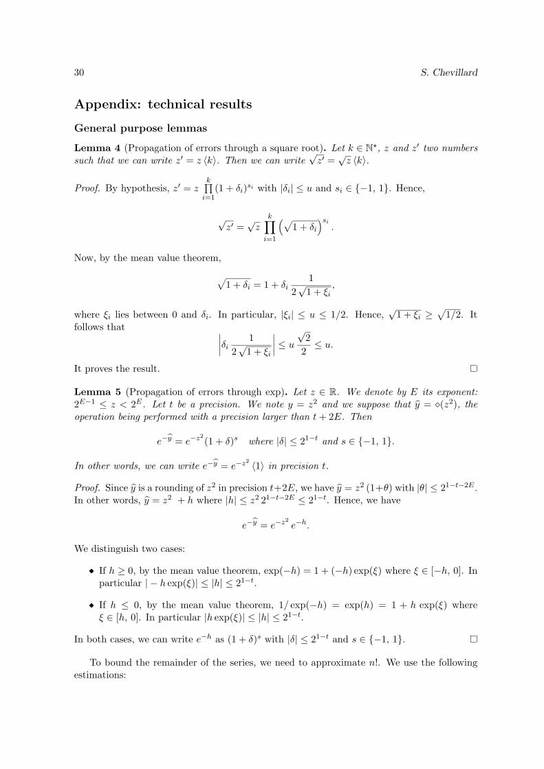
Lemma 4 (Propagation of errors through a square root). Let k ∈ N⋆, z and z′ two numberssuch that we can write z′ = z 〈k〉. Then we can write
√z′ =
√z 〈k〉.
Proof. By hypothesis, z′ = zk∏i=1
(1 + δi)si with |δi| ≤ u and si ∈ {−1, 1}. Hence,
√z′ =
√zk∏
i=1
(√1 + δi
)si.
Now, by the mean value theorem,
√1 + δi = 1 + δi
1
2√
1 + ξi,
where ξi lies between 0 and δi. In particular, |ξi| ≤ u ≤ 1/2. Hence,√
1 + ξi ≥√
1/2. Itfollows that ∣∣∣∣δi
1
2√
1 + ξi
∣∣∣∣ ≤ u√
2
2≤ u.
It proves the result.
Lemma 5 (Propagation of errors through exp). Let z ∈ R. We denote by E its exponent:2E−1 ≤ z < 2E. Let t be a precision. We note y = z2 and we suppose that y = ⋄(z2), theoperation being performed with a precision larger than t+ 2E. Then
e−y = e−z2
(1 + δ)s where |δ| ≤ 21−t and s ∈ {−1, 1}.
In other words, we can write e−y = e−z2 〈1〉 in precision t.
Proof. Since y is a rounding of z2 in precision t+2E, we have y = z2 (1+θ) with |θ| ≤ 21−t−2E .In other words, y = z2 + h where |h| ≤ z2 21−t−2E ≤ 21−t. Hence, we have
e−y = e−z2
e−h.
We distinguish two cases:
❼ If h ≥ 0, by the mean value theorem, exp(−h) = 1 + (−h) exp(ξ) where ξ ∈ [−h, 0]. Inparticular | − h exp(ξ)| ≤ |h| ≤ 21−t.
❼ If h ≤ 0, by the mean value theorem, 1/ exp(−h) = exp(h) = 1 + h exp(ξ) whereξ ∈ [h, 0]. In particular |h exp(ξ)| ≤ |h| ≤ 21−t.
In both cases, we can write e−h as (1 + δ)s with |δ| ≤ 21−t and s ∈ {−1, 1}.
To bound the remainder of the series, we need to approximate n!. We use the followingestimations:
erf and erfc in arbitrary precision 31
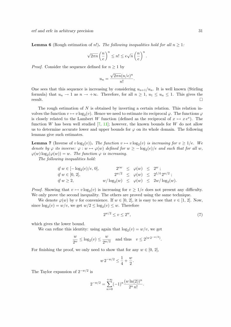
Lemma 6 (Rough estimation of n!). The following inequalities hold for all n ≥ 1:
√2πn
(n
e
)n≤ n! ≤ e
√n
(n
e
)n.
Proof. Consider the sequence defined for n ≥ 1 by
un =
√2πn(n/e)n
n!.
One sees that this sequence is increasing by considering un+1/un. It is well known (Stirlingformula) that un → 1 as n → +∞. Therefore, for all n ≥ 1, u1 ≤ un ≤ 1. This gives theresult.
The rough estimation of N is obtained by inverting a certain relation. This relation in-volves the function v 7→ v log2(v). Hence we need to estimate its reciprocal ϕ. The functions ϕis closely related to the Lambert W function (defined as the reciprocal of x 7→ x ex). Thefunction W has been well studied [7, 11]; however, the known bounds for W do not allowus to determine accurate lower and upper bounds for ϕ on its whole domain. The followinglemmas give such estimates.
Lemma 7 (Inverse of v log2(v)). The function v 7→ v log2(v) is increasing for v ≥ 1/e. Wedenote by ϕ its inverse: ϕ : w 7→ ϕ(w) defined for w ≥ − log2(e)/e and such that for all w,ϕ(w) log2(ϕ(w)) = w. The function ϕ is increasing.
The following inequalities hold:
if w ∈ [− log2(e)/e, 0], 2ew ≤ ϕ(w) ≤ 2w ;
if w ∈ [0, 2], 2w/2 ≤ ϕ(w) ≤ 21/4 2w/2 ;
if w ≥ 2, w/ log2(w) ≤ ϕ(w) ≤ 2w/ log2(w).
Proof. Showing that v 7→ v log2(v) is increasing for v ≥ 1/e does not present any difficulty.We only prove the second inequality. The others are proved using the same technique.
We denote ϕ(w) by v for convenience. If w ∈ [0, 2], it is easy to see that v ∈ [1, 2]. Now,since log2(v) = w/v, we get w/2 ≤ log2(v) ≤ w. Therefore
2w/2 ≤ v ≤ 2w, (7)
which gives the lower bound.We can refine this identity: using again that log2(v) = w/v, we get
w
2w≤ log2(v) ≤ w
2w/2and thus v ≤ 2(w 2−w/2).
For finishing the proof, we only need to show that for any w ∈ [0, 2],
w 2−w/2 ≤ 1
4+w
2.
The Taylor expansion of 2−w/2 is
2−w/2 =+∞∑
n=0
(−1)n(w ln(2))n
2n n!.
32 S. Chevillard
The series is alternating with a decreasing general term when w ∈ [0, 2]. Hence
2−w/2 ≤ 1− w ln(2)
2+w2 ln(2)2
8.
From this inequality, we deduce
w 2−w/2 − w2≤ w
(1
2− w ln(2)
2+w2 ln(2)2
8
).
Studying the variations of the right-hand term of this inequality, we get
w 2−w/2 − w2≤ 4
27 ln(2)≃ 0.2137 · · · ≤ 1/4.
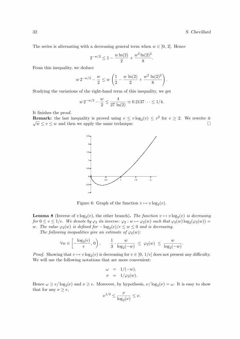
It finishes the proof.Remark: the last inequality is proved using v ≤ v log2(v) ≤ v2 for v ≥ 2. We rewrite it√w ≤ v ≤ w and then we apply the same technique.
Figure 6: Graph of the function v 7→ v log2(v).
Lemma 8 (Inverse of v log2(v), the other branch). The function v 7→ v log2(v) is decreasingfor 0 ≤ v ≤ 1/e. We denote by ϕ2 its inverse: ϕ2 : w 7→ ϕ2(w) such that ϕ2(w) log2(ϕ2(w)) =w. The value ϕ2(w) is defined for − log2(e)/e ≤ w ≤ 0 and is decreasing.
The following inequalities give an estimate of ϕ2(w):
∀w ∈[− log2(e)
e, 0
),
1
3· w
log2(−w)≤ ϕ2(w) ≤ w
log2(−w).
Proof. Showing that v 7→ v log2(v) is decreasing for v ∈ [0, 1/e] does not present any difficulty.We will use the following notations that are more convenient:
ω = 1/(−w),
ν = 1/ϕ2(w).
Hence ω ≥ e/ log2(e) and ν ≥ e. Moreover, by hypothesis, ν/ log2(ν) = ω. It is easy to showthat for any ν ≥ e,
ν1/3 ≤ ν
log2(ν)≤ ν.
erf and erfc in arbitrary precision 33
Therefore, ω ≤ ν ≤ ω3 and thus log2(ω) ≤ log2(ν) ≤ 3 log2(ω). We conclude by usingν = ω log2(ν).
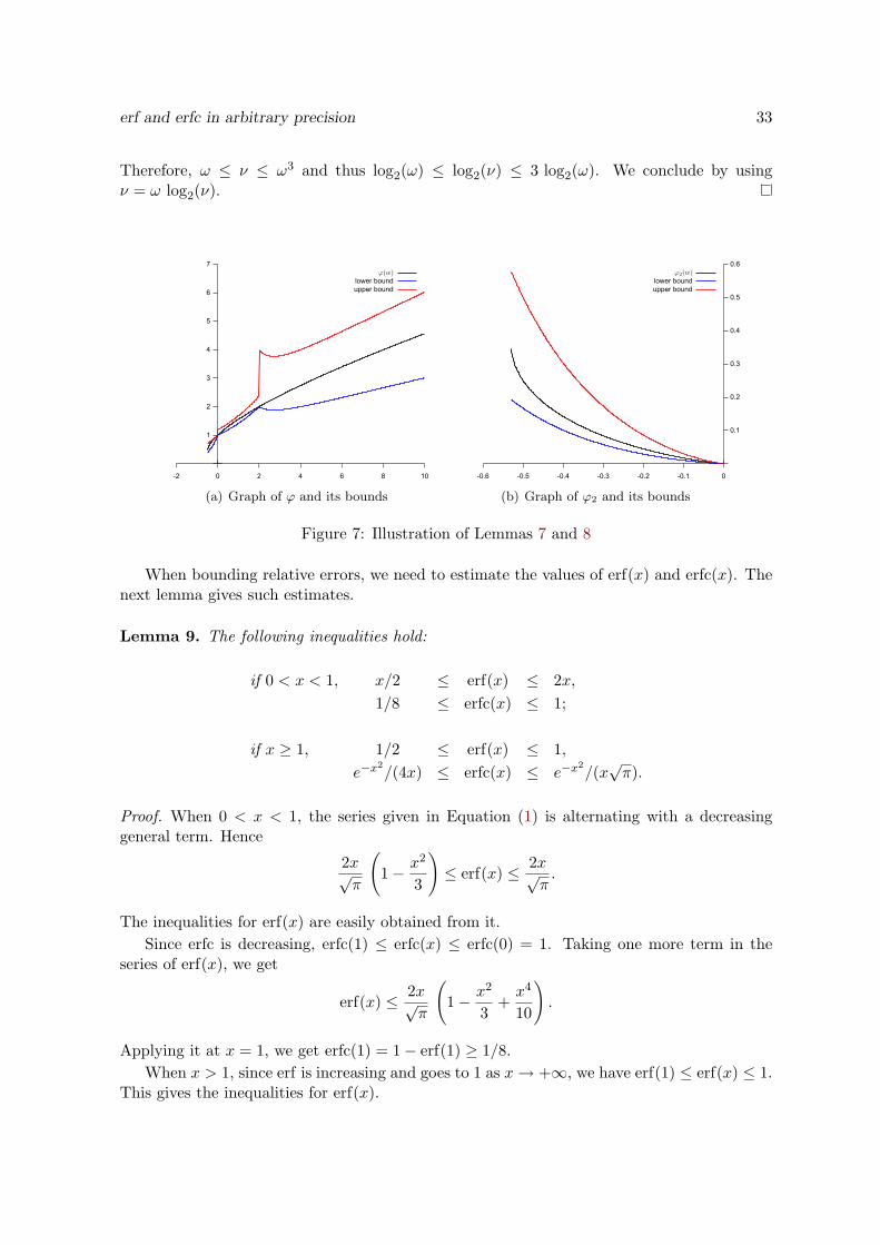
(a) Graph of ϕ and its bounds (b) Graph of ϕ2 and its bounds
Figure 7: Illustration of Lemmas 7 and 8
When bounding relative errors, we need to estimate the values of erf(x) and erfc(x). Thenext lemma gives such estimates.
Lemma 9. The following inequalities hold:
if 0 < x < 1, x/2 ≤ erf(x) ≤ 2x,
1/8 ≤ erfc(x) ≤ 1;
if x ≥ 1, 1/2 ≤ erf(x) ≤ 1,
e−x2
/(4x) ≤ erfc(x) ≤ e−x2
/(x√π).
Proof. When 0 < x < 1, the series given in Equation (1) is alternating with a decreasinggeneral term. Hence
2x√π
(1− x
2
3
)≤ erf(x) ≤ 2x√
π.
The inequalities for erf(x) are easily obtained from it.
Since erfc is decreasing, erfc(1) ≤ erfc(x) ≤ erfc(0) = 1. Taking one more term in theseries of erf(x), we get
erf(x) ≤ 2x√π
(1− x
2
3+x4
10
).
Applying it at x = 1, we get erfc(1) = 1− erf(1) ≥ 1/8.
When x > 1, since erf is increasing and goes to 1 as x→ +∞, we have erf(1) ≤ erf(x) ≤ 1.This gives the inequalities for erf(x).
34 S. Chevillard
We now prove the last two inequalities of the lemma. By definition,
erfc(x) =2√π
∫ +∞
xe−v
2
dv
=2√π
∫ +∞
x
−2v e−v2
−2vdv
=2√π
(e−x
2
2x−∫ +∞
x
e−v2
2v2dv
).
This gives the upper bound. For the lower bound, we use the change of variable v ← v + x:
∫ +∞
x
e−v2
2v2dv =
∫ +∞
0
e−x2−2vx−v2
2(v + x)2dv.
Since (v + x)2 ≥ x2 and −v2 ≤ 0,
∫ +∞
0
e−x2−2vx−v2
2(v + x)2dv ≤ e
−x2
2x2
∫ +∞
0e−2vx dv =
e−x2
4x3.
Therefore,
erfc(x) ≥ e−x2
x√π
(1− 1
2x2
)
≥ e−x2
x 2√π
since x ≥ 1.
We conclude by remarking that 2√π ≃ 3.544 ≤ 4.
Results related to the implementation of Equation (1)
Proposition 3. Let E be the exponent of x. If N satisfies
N
ex2log2
(N
ex2
)≥ t′ + max(0, E)
ex2,
the remainder ε(1)N is bounded by 2−t
′−1 erf(x).
Proof. Remark first that for N ≥ 1,
2√π· 1
(2N + 1)√
2πN≤ 1
4. (8)
We distinguish the cases when x < 1 and when x ≥ 1:
❼ if x < 1, E ≤ 0 and erf(x) is greater than x/2. The hypothesis becomes (ex2/N)N ≤ 2−t′
and thusx2N+1
2
(e
N
)N≤ 2−t
′
erf(x). (9)
erf and erfc in arbitrary precision 35
❼ if x ≥ 1, E > 0 and erf(x) is greater than 1/2. The hypothesis becomes (ex2/N)N ≤2−t
′−E and thusx2N
2
(e
N
)N≤ 2−t
′−E erf(x).
Since x < 2E we obtain Inequality (9) again.
From Inequalities (8) and (9) we deduce that
2√π· x
2N+1
2N + 1
(e
N
)N 1√2πN
≤ 2−t′−1 erf(x).
Using Lemma 6, we get
2√π· x2N+1
(2N + 1)N !≤ 2−t
′−1 erf(x).
Remark that the left term of the inequality is the absolute value of the general term ofthe series. Since it is smaller than 2−t
′−1 erf(x), it is in particular smaller than 1/2. Since theseries is alternating, we can bound the remainder by the absolute value of the first neglectedterm as soon as the term decreases in absolute value.
In our case, the absolute value of the general term may begin by increasing before de-creasing. But when it increases, it is always greater than 1. Therefore, since here it is smaller
than 1/2, we are in the decreasing phase and we can write ε(1)N (x) ≤ 2−t
′−1 erf(x).
Recipe 1. We first evaluate a = (t′+ max(0, E))/(ex2). In fact, when performing the evalu-ation, the rounding modes are carefully chosen in such a way that one gets an overestimationau of a: au ≥ a. Then, N is chosen according to the following recipe:
– if au ≥ 2, N ≥ (ex2) 2au/ log2(au) ;
– if au ∈ [0, 2], N ≥ (ex2) 21/4 2au/2.
These formulas are evaluated with appropriate rounding modes, in order to ensure that Nis really greater than the actual value.
Proof. Proposition 3 gives a sufficient condition on N that ensures that ε(1)N is bounded by
2−t′−1 erf(x). We reason by sufficient conditions:
❼ from Proposition 3, it suffices that
N
ex2log2
(N
ex2
)≥ a ;
❼ hence, it suffices thatN
ex2log2
(N
ex2
)≥ au ;
❼ this inequality can be inverted with help of function ϕ (defined in Lemma 7). Namely,we have N/(ex2) ≥ ϕ(au);
❼ for obtaining this inequality, it suffices that N/(ex2) be greater than an upper boundof ϕ(au). Such an upper bound is given by Lemma 7. The recipe follows.
36 S. Chevillard
Proposition 4. If Algorithm 3 is used to compute an approximation S(x) of the sum S(x),the following holds:
S(x) =N−1∑
n=0
(−1)n2x√π· x2n
(2n+ 1)n!〈8N〉 .
Thus∣∣∣S(x)− S(x)
∣∣∣ ≤ γ8N(
2x√π
N−1∑
n=0
x2n
(2n+ 1)n!
)≤ γ8N
2√π
∫ x
0ev
2
dv.
The bound γ8N could be made tighter. However, we cannot hope a better value than γNsince we do O(N) operations. Only the logarithm of this value will be of interest for choosingthe working precision t. By working more carefully, we would not get more than replacinglog(8N) by log(N) and it would not be of any practical benefit.
Proof. To prove this result, we use the same techniques as those presented in the example ofSection 3. The main arguments are the following.
❼ Line 1 of the algorithm leads to one error;
❼ Line 4 is obtained by binary exponentiation: by counting the number of multiplications,it is easy to show that z = z 〈2L− 1〉;
❼ Line 6 involves an approximation of π (π = π 〈1〉) and a square root. Using Lemma 4we get acc = ⋄(
√π) = ⋄(√π 〈1〉) =
√π 〈2〉;
❼ Line 7 involves a division (the multiplication by 2 is exact);
❼ acc is updated at lines 16 and 20 of the algorithm. At line 16, it accumulates 2L errors(2L − 1 due to z and one due to the multiplication itself). At line 20, it accumulatesone error. It is hence easy to show that we can always write
acc = acc 〈 3︸︷︷︸initialization
+ N︸︷︷︸line 20 occurs at most N times
+ 2L⌊N/L⌋︸ ︷︷ ︸line 16 occurs at most ⌊N/L⌋ times
〉.
We simplify it in acc = acc 〈3 + 3N〉;
❼ We can always write tmp = tmp 〈4 + 3N〉 since tmp is obtained from acc by one division(2k + 1 is computed exactly in integer arithmetic);
❼ Eventually, S[i] is obtained by less than N additions using variable tmp which allowsto write
Si = tmpi 〈4N + 4〉+ tmpi+L 〈4N + 4〉+ · · ·+ tmpi+N−L 〈4N + 4〉
where tmpk denotes the value of variable tmp at step k of the algorithm;
❼ The evaluation by Horner’s rule at line 25 accumulates 3 more errors per step (one comesfrom the fact that y = x2 〈1〉, one comes from the multiplication and one comes fromthe addition). Therefore, during the complete loop, 3(L−1) errors are accumulated perterm of the sum. We bound it by 3N − 3 and finally get the result with 〈7N + 1〉. Webound it by 〈8N〉.
erf and erfc in arbitrary precision 37
The value(∫ x
0 ev2
dv)
quantifies the catastrophic cancellations that appear when Equa-
tion (1) is used for evaluating erf(x). The following lemma allows us to bound it.
Lemma 10. The following inequalities hold:
if 0 < x < 1, x ≤∫ x
0ev
2
dv ≤ 2x;
if x ≥ 1,1
e2· ex2
x≤
∫ x
0ev
2
dv ≤ ex2
x.
Proof. For the first inequality, the lower bound is obtained by replacing ev2
by 1 in the integral.The upper bound is obtained by replacing ev
2
by e0.552
on [0, 0.55] and by e on [0.55, 1].For the second inequality, the upper bound is obtained by replacing ev
2
by evx in theintegral. The lower bound is obtained by considering the integral restricted to the interval[x− 1/x, x].
Recipe 2. Let E be the exponent of x. For the evaluation of erf(x) by Equation (1), anappropriate working precision t is
– when x < 1, t ≥ t′ + 9 + ⌈log2N⌉ ;
– when x ≥ 1, t ≥ t′ + 9 + ⌈log2N⌉ − E + x2 log2(e).
In practice log2(e) is replaced by a value precomputed with rounding upwards. The factorx2 log2(e) that appears when x > 1 highlights the fact that the series is ill-conditioned forlarge values of x.
Proof. We show the result for the first inequality. The second one is obtained the same way.We suppose that 0 < x < 1 and t ≥ t′ + 9 + ⌈log2N⌉. Thus
2−t+8N ≤ 2−t′−1.
Using the fact that γ8N ≤ 16Nu (Proposition 2), we get
2γ8N (2x) ≤ 2−t′−1 x
2.
We conclude by using (x/2) ≤ erf(x) (Lemma 9), (2/√π) ≤ 2 and
∫ x
0ev
2
dv ≤ 2x (Lemma 10).
Results related to the implementation of Equation (2)
The first thing we need is a way of bounding the remainder. This is achieved by thefollowing lemma:
Lemma 11. If N ≥ 2x2, the following inequality holds:
ε(2)N (x) ≤ 2
2xe−x2
√π· (2x2)n
1 · 3 · · · (2N + 1).
38 S. Chevillard
Proof. By definition,
ε(2)N (x) =
2xe−x2
√π
+∞∑
n=N
(2x2)n
1 · 3 · · · (2n+ 1)
=2xe−x
2
√π· (2x2)N
1 · 3 · · · (2N + 1)
(1 +
2x2
2N + 3+
(2x2)2
(2N + 3)(2N + 5)+ · · ·
).
We bound it by the geometric series with a common ratio of (2x2)/(2N + 3) and a first termequal to 1:
ε(2)N (x) ≤ 2xe−x
2
√π· (2x2)N
1 · 3 · · · (2N + 1)
(1 +
2x2
2N + 3+
(2x2)2
(2N + 3)(2N + 3)+ · · ·
)
Since N ≥ 2x2, (2x2)/(2N + 3) ≤ 1/2 and the sum of the series is bounded by 2.
Proposition 5. Let E be the exponent of x. If N satisfies N ≥ 2x2 and
N
ex2log2
(N
ex2
)≥ t′ + 3 + max(0, E)− x2 log2(e)
ex2
the remainder is bounded by erf(x) 2−t′−1.
Proof. We use the same kind of arguments as for Proposition 3. The product 1 ·3 · · · (2N +1)is equal to (2N + 1)!/(2N N !). This lets us write
∣∣∣ε(2)N (x)
∣∣∣ ≤ 4xe−x
2
√π· (2x2)N N ! 2N
(2N + 1)!≤ 4xe−x
2
√π· (2x2)N N ! 2N
(2N)!.
We conclude using Lemmas 6 and 9.
Recipe 3. We deduce the formulas for computing an overestimation of N :
– if au ≥ 2, take N ≥ (ex2) 2au/ log2(au) ;
– if au ∈ [0, 2], take N ≥ (ex2) 21/4 2au/2 ;
– if au < 0, let N0 ≥ (ex2) 2au and perform the following test:
– if N0 ≥ 2x2, take N = N0,
– else take N = ⌈2x2⌉.
Only the case au < 0 could lead to a value N smaller than 2x2. If it is the case, we takeN = ⌈2x2⌉, in order to ensure the hypothesis of Proposition 5.
Proof. The proof is similar to the proof of Recipe 1.
Proposition 6. If Algorithm 4 is used to compute an approximation S(x) of the sum S(x),the following holds:
S(x) =N−1∑
n=0
2xe−x2
√π· (2x2)n
1 · 3 · · · (2n+ 1)〈16N〉 .
Thus ∣∣∣S(x)− S(x)∣∣∣ ≤ γ16N S(x) ≤ γ16N erf(x).
erf and erfc in arbitrary precision 39
Proof. In fact, using the same techniques as in Proposition 4, one proves that
S(x) =N−1∑
n=0
2xe−x2
√π· (2x2)n
1 · 3 · · · (2n+ 1)〈7N + 3〉 .
We bound it by 〈16N〉 because it is more convenient to use powers of 2.Note that at line 9 of the algorithm, x2 is computed in precision t + max(2E, 0). Using
Lemma 5, it allows for writing α0 = α0 〈6〉.
Results related to the evaluation of erfc(x) by Equations (1) and (2)
Lemma 1. If s is chosen according to the following recipe, |R− erf(x)| ≤ 2−t′−1 erfc(x).
– If x ≤ −1, s ≥ t′ + 1 ;
– if − 1 < x < 0, s ≥ t′ + 2 + E ;
– if 0 ≤ x < 1, s ≥ t′ + 5 + E ;
– if x ≥ 1, s ≥ t′ + 3 + E + x2 log2(e).
Proof.First case.
We suppose x ≤ −1 and s ≥ t′ + 1. From the hypotheses we get
∣∣R− erf(x)∣∣ ≤ 2−s | erf(x)| ≤ 2−t
′−1 | erf(x)|.
Since x < 0, erfc(x) ≥ 1. Moreover, | erf(x)| ≤ 1. This gives the result.
Second case.
We suppose −1 < x < 0 and s ≥ t′ + 2 + E. From the hypotheses we get
∣∣R− erf(x)∣∣ ≤ 2−s | erf(x)| ≤ 2−t
′−1 2−E−1 | erf(x)|.
Since x < 0, erfc(x) ≥ 1. Moreover, | erf(x)| = erf(|x|) ≤ 2|x| ≤ 2E+1. This gives the result.
Third case.
It is the same as the second case but using erfc(x) ≥ 1/8.
Fourth case.
Here x ≥ 1 and s ≥ t′ + 3 + E + x2 log2(e). Hence
∣∣R− erf(x)∣∣ ≤ 2−s erf(x) ≤ 2−t
′−1 2−E−2 e−x2 | erf(x)|.
Since x ≥ 1, erf(x) ≤ 1 and erfc(x) ≥ e−x2
/(4x) ≥ e−x2
/(4 2E). This gives the result.
Results related to the implementation of Equation (3)
Lemma 12. The following inequality holds for any x ≥ 1:
|ε(3)N (x)| ≤ e
−x2
x
(N
ex2
)N.
40 S. Chevillard
Proof. The result is obtained from the bound given in Equation (4). The product 1·3 · · · (2N−1) is equal to (2N)!/(2N N !). We conclude using the bounds given in Lemma 6.
Proposition 7. If N satisfies
N
ex2log2
(N
ex2
)≤ −t
′ − 3
ex2
the remainder is bounded by erfc(x) 2−t′−1.
Proof. We use the previous lemma and the inequality erfc(x) ≥ e−x2
/(4x) given in Lemma 9.
Recipe 5. The rule for computing N is the following: first, we compute a = (−t′ − 3)/ex2
choosing the rounding modes for obtaining a underestimation ad of a and then we choose Naccording to the following recipe:
– if ad < − log2(e)/e, Equation (3) cannot be used;
– else let N0 ≥ (ex2) ad/ log2(−ad) and perform the following test:
– if N0 ≤ x2, let N = N0,
– else let N1 ≃ x2 and perform the following test:
– ifN1
ex2log2
(N1
ex2
)≤ ad, let N = N1,
– else, Equation (3) cannot be used.
Of course the value − log2(e)/e is evaluated in such a way that we get an overestimationof the actual value. Also, in the test N0 ≤ x2, the value x2 is replaced by an underestimation.
Proof. It is the same technique as in the proof of Recipe 1. Lemma 8 is used to invert theequation of Proposition 7.
Proposition 8. If Algorithm 5 is used to compute an approximation S(x) of the sum S(x),the following holds:
∣∣∣S(x)− S(x)∣∣∣ ≤ γ16N
e−x2
x√π· 3
2.
Proof. In this algorithm, y = y 〈2〉, hence the binary exponentiation leads to
z = z 〈3L− 1〉 .
Using the same technique as in the proof of Proposition 4, we get the bound
S(x) =e−x
2
x√π〈8N + 3〉+
N−1∑
n=1
(−1)ne−x
2
x√π· 1 · 3 · · · (2n− 1)
(2x2)n〈8N + 3〉 .
We bound 〈8N + 3〉 by 〈16N〉 and thus obtain
∣∣∣S(x)− S(x)∣∣∣ ≤ γ16N
e−x2
x√π
(1 +
N−1∑
n=1
1 · 3 · · · (2n− 1)
(2x2)n
).
erf and erfc in arbitrary precision 41
We now prove that
1 +N−1∑
n=1
1 · 3 · · · (2n− 1)
(2x2)n≤ 3
2for N ≤ ⌊x2 + 1/2⌋.
Since N ≤ ⌊x2 + 1/2⌋, N ≤ x2 + 1. Moreover, the general term is decreasing. Hence, we canwrite
N−1∑
n=1
1 · 3 · · · (2n− 1)
(2x2)n≤ (N − 1)
1
2x2≤ 1
2.
Results related to the implementation of erf(x) by Equation (3)
Lemma 2. If x ≥ 1, the inequality |R− erfc(x)| ≤ 2−t′−1 erfc(−x) holds when s is chosen
according to the following recipe:
s ≥ t′ + 2− E − x2 log2(e).
Proof. Since s ≥ t′+ 2−E− x2 log2(e), we have 2−s ≤ 2−t′−1 2E−1 ex
2
. Moreover, we alwayshave 2E−1 ≤ x and by Lemma 9
erfc(x) ≤ e−x2
x√π≤ e−x2
x.
By definition, |R − erfc(x)| ≤ 2−s erfc(x), thus |R − erfc(x)| ≤ 2−t′−1. We conclude by
remarking that erfc(−x) ≥ 1 since x ≥ 0.
Lemma 3. If x ≥ 1 the inequality |R− erfc(x)| ≤ 2−t′−1 erf(x) holds when s is chosen
according to the following recipe:
s ≥ t′ + 3− E − x2 log2(e).
Proof. We proceed the same way as in the previous proof. Hence we get
|R− erfc(x)| ≤ 2−t′−1 1
2.
Since x ≥ 1, Lemma 9 indicates that erf(x) ≥ 1/2, which concludes the proof.