1

The First Carrier Phase Tracking and PositioningResults with Starlink LEO Satellite Signals

Joe Khalife,Member, IEEE, Mohammad Neinavaie,Student Member, IEEE,and Zaher M. Kassas,Senior Member, IEEE

Abstract—This letter shows the first carrier phase trackingand positioning results with Starlink’s low Earth orbit (LE O)satellite signals. An adaptive Kalman filter (KF)-based algorithmfor tracking the beat carrier phase from the unknown Starlinksignals is proposed. Experimental results show carrier phasetracking of six Starlink satellites and a horizontal positioningerror of 7.7 m.

Index Terms—signals of opportunity, carrier phase positioning,low Earth orbit, Starlink.

I. I NTRODUCTION

Low Earth orbit (LEO) broadband communication satellitesignals have been considered as possible reliable sources fornavigation by various theoretical and experimental studies[1]–[4]. With SpaceX having launched more than a thousandspace vehicles (SVs) into LEO, a renaissance in LEO-basednavigation has started. Signals from LEO SVs are receivedwith higher power compared to medium Earth orbit (MEO)where GNSS SVs reside. Moreover, LEO SVs are moreabundant than GNSS SVs to make up for the reduced footprint,and their signals are spatially and spectrally diverse.

Opportunistic navigation frameworks with LEO SV signalshave drawn attention recently as they do not require additional,costly services or infrastructure from the broadband provider[5]. One major requirement in such frameworks is the abilityto draw navigation observables from these LEO SV signalsof opportunity. However, broadband providers do not usuallydisclose the transmitted signal structure to protect theirintel-lectual property. As such, one would have to dissect LEO SVsignals to draw navigation observables. A cognitive approachto tracking the Doppler frequency of unknown terrestrialsignals was proposed in [6]. This method cannot be adoptedhere as it does not account for the very-high Doppler dueLEO SV dynamics and requires knowledge of the period ofthe beacon within the transmitted signal, which is unknown inthe case of Starlink LEO SVs. This letter develops a carrierphase tracking algorithm for Starlink signals without priorknowledge of their structure.

This work was supported in part by the Office of Naval Research(ONR)under Grant N00014-19-1-2511; in part by the National Science Founda-tion (NSF) under Grant 1929965; and in part by the U.S. Department ofTransportation (USDOT) under Grant 69A3552047138 for the CARMENUniversity Transportation Center (UTC).

J. Khalife and M. Neinavaie are with the Department of Mechani-cal and Aerospace Engineering at the University of California, Irvine(UCI), USA. Z. M. Kassas is with Department of Mechanical andAerospace Engineering at UCI and holds a joint appointment at TheOhio State University, U.S.A. Address: 27 E Peltason Dr, Irvine, CA92697, USA (email:khalifej@uci.edu, mneinava@uci.edu, andzkassas@ieee.org). Corresponding author: Z. Kassas.

Recent efforts in carrier synchronization showed the ben-efit of using Kalman filter (KF)-based tracking loops overtraditional Costas-based phase-locked loops (PLLs) [7]–[10].These adaptive methods either (i) update the process noisecovariance using the residuals or (ii) update the measurementnoise covariance using the carrier-to-noise ratio. However,high fluctuations in the process noise covariance may causethe filter to diverge [10]. Moreover, the carrier-to-noise ratiocannot be reliably estimated when the signal structure isunknown, as is the case with Starlink signals.

This letter makes the following contributions. First, the Star-link signals are analyzed and a model suitable for carrier phasetracking is developed. Second, an adaptive KF-based trackingloop is developed where the measurement noise is updatedbased on a heuristic of the residuals. Third, a demonstrationof the first carrier phase tracking and positioning results withreal Starlink signals is presented, showing a horizontal positionerror of 7.7 m with six Starlink SVs.

II. RECEIVED SIGNAL MODEL

In this letter, all signals are represented as complex signals(both in-phase and quadrature baseband components).

A. Starlink Downlink Signals

Little is known about Starlink downlink signals or theirair interface in general, except for the channel frequenciesand bandwidths. One cannot readily design a receiver to trackStarlink signals with the aforementioned information onlyasa deeper understanding of the signals is needed. Software-defined radios (SDRs) come in handy in such situations, sincethey allow one to sample bands of the radio frequency spec-trum. However, there are two main challenges for samplingStarlink signals: (i) the signals are transmitted in Ku/Ka-bands, which is beyond the carrier frequencies that mostcommercial SDRs can support, and (ii) the downlink channelbandwidths can be up to 240 MHz, which also surpasses thecapabilities of current commercial SDRs. The first challengecan be resolved by using a mixer/downconverter between theantenna and the SDR. However, the sampling bandwidth canonly be as high as the SDR allows. In general, opportunisticnavigation frameworks do not require much information fromthe communication/navigation source (e.g., decoding telemetryor ephemeris data or synchronizing to a certain preamble).Therefore, the aim of the receiver is to exploit enough of thedownlink signal to be able produce raw navigation observables(e.g., Doppler and carrier phase). Fortunately, a look at theFFT of the downlink signal at 11.325 GHz carrier frequency

Preprint of article accepted for publication in IEEE Transactions on Aerospace and Electronic Systems

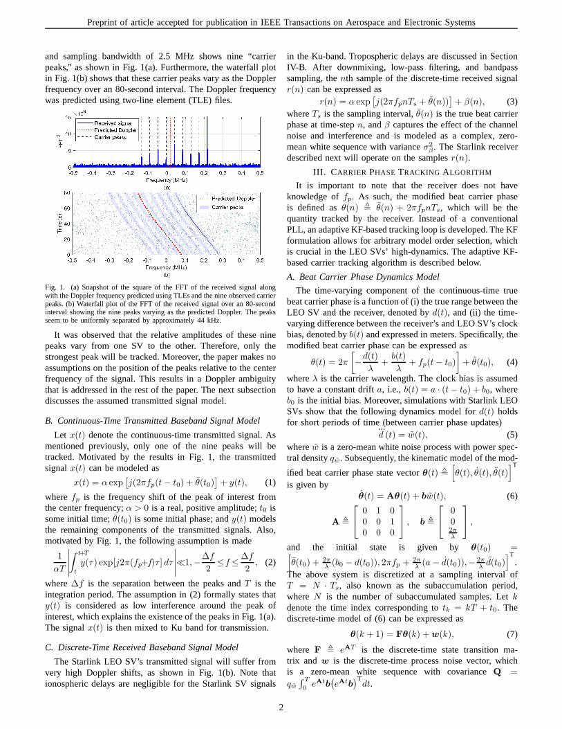
and sampling bandwidth of 2.5 MHz shows nine “carrierpeaks,” as shown in Fig. 1(a). Furthermore, the waterfall plotin Fig. 1(b) shows that these carrier peaks vary as the Dopplerfrequency over an 80-second interval. The Doppler frequencywas predicted using two-line element (TLE) files.

Fig. 1. (a) Snapshot of the square of the FFT of the received signal alongwith the Doppler frequency predicted using TLEs and the nineobserved carrierpeaks. (b) Waterfall plot of the FFT of the received signal over an 80-secondinterval showing the nine peaks varying as the predicted Doppler. The peaksseem to be uniformly separated by approximately 44 kHz.

It was observed that the relative amplitudes of these ninepeaks vary from one SV to the other. Therefore, only thestrongest peak will be tracked. Moreover, the paper makes noassumptions on the position of the peaks relative to the centerfrequency of the signal. This results in a Doppler ambiguitythat is addressed in the rest of the paper. The next subsectiondiscusses the assumed transmitted signal model.

B. Continuous-Time Transmitted Baseband Signal Model

Let x(t) denote the continuous-time transmitted signal. Asmentioned previously, only one of the nine peaks will betracked. Motivated by the results in Fig. 1, the transmittedsignalx(t) can be modeled as

x(t) = α exp[

j(2πfp(t− t0) + θ(t0)]

+ y(t), (1)

wherefp is the frequency shift of the peak of interest fromthe center frequency;α > 0 is a real, positive amplitude;t0 issome initial time;θ(t0) is some initial phase; andy(t) modelsthe remaining components of the transmitted signals. Also,motivated by Fig. 1, the following assumption is made

1

αT

∣

∣

∣

∣

∣

∫ t+T

t

y(τ) exp[j2π(fp+f)τ ] dτ

∣

∣

∣

∣

∣

≪1,−∆f

2≤f≤

∆f

2, (2)

where∆f is the separation between the peaks andT is theintegration period. The assumption in (2) formally states thaty(t) is considered as low interference around the peak ofinterest, which explains the existence of the peaks in Fig. 1(a).The signalx(t) is then mixed to Ku band for transmission.

C. Discrete-Time Received Baseband Signal Model

The Starlink LEO SV’s transmitted signal will suffer fromvery high Doppler shifts, as shown in Fig. 1(b). Note thationospheric delays are negligible for the Starlink SV signals

in the Ku-band. Tropospheric delays are discussed in SectionIV-B. After downmixing, low-pass filtering, and bandpasssampling, thenth sample of the discrete-time received signalr(n) can be expressed as

r(n) = α exp[

j(2πfpnTs + θ(n))]

+ β(n), (3)whereTs is the sampling interval,θ(n) is the true beat carrierphase at time-stepn, andβ captures the effect of the channelnoise and interference and is modeled as a complex, zero-mean white sequence with varianceσ2

β . The Starlink receiverdescribed next will operate on the samplesr(n).

III. C ARRIER PHASE TRACKING ALGORITHM

It is important to note that the receiver does not haveknowledge offp. As such, the modified beat carrier phaseis defined asθ(n) , θ(n) + 2πfpnTs, which will be thequantity tracked by the receiver. Instead of a conventionalPLL, an adaptive KF-based tracking loop is developed. The KFformulation allows for arbitrary model order selection, whichis crucial in the LEO SVs’ high-dynamics. The adaptive KF-based carrier tracking algorithm is described below.

A. Beat Carrier Phase Dynamics Model

The time-varying component of the continuous-time truebeat carrier phase is a function of (i) the true range betweentheLEO SV and the receiver, denoted byd(t), and (ii) the time-varying difference between the receiver’s and LEO SV’s clockbias, denoted byb(t) and expressed in meters. Specifically, themodified beat carrier phase can be expressed as

θ(t) = 2π

[

−d(t)

λ+

b(t)

λ+ fp(t− t0)

]

+ θ(t0), (4)

whereλ is the carrier wavelength. The clock bias is assumedto have a constant drifta, i.e., b(t) = a · (t− t0) + b0, whereb0 is the initial bias. Moreover, simulations with Starlink LEOSVs show that the following dynamics model ford(t) holdsfor short periods of time (between carrier phase updates)...

d (t) = w(t), (5)wherew is a zero-mean white noise process with power spec-tral densityqw. Subsequently, the kinematic model of the mod-

ified beat carrier phase state vectorθ(t) ,[

θ(t), θ(t), θ(t)]T

is given byθ(t) = Aθ(t) + bw(t), (6)

A ,

0 1 00 0 10 0 0

, b ,

002πλ

,

and the initial state is given by θ(t0) =[

θ(t0) +2πλ(b0 − d(t0)), 2πfp +

2πλ(a− d(t0)),−

2πλd(t0)

]T

.The above system is discretized at a sampling interval ofT = N · Ts, also known as the subaccumulation period,whereN is the number of subaccumulated samples. Letk

denote the time index corresponding totk = kT + t0. Thediscrete-time model of (6) can be expressed as

θ(k + 1) = Fθ(k) +w(k), (7)

where F , eAT is the discrete-time state transition ma-trix and w is the discrete-time process noise vector, whichis a zero-mean white sequence with covarianceQ =

qw∫ T

0eAtb

(

eAtb)T

dt.

2

Preprint of article accepted for publication in IEEE Transactions on Aerospace and Electronic Systems

B. Adaptive KF-Based Carrier Tracking

The adaptive KF-based tracking algorithm operates in asimilar fashion to Costas loops, except that the loop filter isreplaced with a KF, where the measurement noise variance isvaried adaptively. Letθ(k|l) denote the KF estimate ofθ(k)given all the measurements up to time-stepl ≤ k, andP(k|l)denote the corresponding estimation error covariance. Theinitial estimate and its corresponding covariance are denotedby θ(0|0) and P(0|0), respectively, and are calculated asdiscussed in Section III-B4. The KF-based tracking algorithmsteps are discussed next.

1) KF Time Update: The standard KF time update equa-tions are preformed to yieldx(k + 1|k) andP(k + 1|k).

2) KF Measurement Update: The KF measurement updatestep is similar to a Costas loop: a carrier wipe-off is firstperformed, followed by an accumulation and discriminationstep. The wipe-off and accumulation are performed as

s(k + 1) =1

N

N−1∑

n=0

r(n+ kN) exp[

−jθ(k + n|k)]

, (8)

where θ(k + n|k) = θ(k|k) +ˆθ(k|k)nTs + 1

2

ˆθ(k|k)(nTs)

2,which is obtained by propagating the initial conditionθ(k|k)by nTs using the dynamics in (6). Since the tracked signal in(3) is dataless, anatan2 discriminator can be used to obtainan estimate of the carrier phase error according to

ν(k + 1) , atan2 (ℑ{s(k + 1)} ,ℜ{s(k + 1)})

= θ(k + 1)− θ(k + 1|k) + v(k + 1), (9)

whereℜ{·} and ℑ{·} denote the real and imaginary parts,respectively, andv(k + 1) is the measurement noise, whichis modeled as a zero-mean, white Gaussian sequence withvarianceσ2

v(k + 1). Since the measurement noise varianceis not known, an estimateσ2

v(k + 1) is used instead in theKF. This estimate is updated adaptively according to the nextsubsection. It is important to note thatν(k + 1) is the KFinnovation and gives a direct measure of the modified beatcarrier phase. Hence, the standard KF measurement updateequations are performed usingν(k + 1), σ2

v(k + 1), and themeasurement matrixH , [1 0 0].

3) Measurement Noise Variance Estimate Update: As thesignal quality fluctuates, it is important to match the measure-ment noise variance to the actual noise statistics. This cannotbe done readily as the channel between the LEO SV and thereceiver is highly dynamic and unknown. Instead, a heuristicmodel is used to updateσ2

v(k) over time, and is given by

σ2v(k + 1) = γσ2

v(k) + (1 − γ)u(k), (10)

where 0 < γ < 1 is a “forgetting” factor (close to one)[11] and u(k) , 1

Kv

∑k

m=k−Kv+1 ν2(m), whereKv is the

number of samples used to estimate the measurement noisevariance. The heuristic model in (10) adapts to the quality ofthe measurements while filtering out abrupt changes in thephase error variance.

4) KF Initialization: The steps above assumed that aninitial estimate and corresponding covariance are available.The initial estimate can be readily obtained from the data.Since a PLL cannot resolve the true initial carrier phase, the

initial estimate θ(0|0) is set to zero with zero uncertainty.This initial ambiguity is accounted for in the navigation filter.Initial estimates of the first and second derivatives ofθ canbe obtained by performing a search over the Doppler and theDoppler rate to maximize the FFT of the received signal. Thesearch yields the Doppler and Doppler rate estimates denoted

by fD(0) and ˆfD(0), respectively. Next, let∆fD and∆fD

denote the sizes of the Doppler and Doppler rate search bins,respectively. It is assumed that the initial Doppler and Dopplerrate errors are uniformly distributed within one bin, and theirinitial probability density functions (pdfs) are bounded byGaussian pdfs with zero-mean and standard deviations∆fD

6

and ∆fD6

, respectively. As such,∆fD and∆fD represent the±3σ intervals of the Gaussian pdfs. The KF is initialized as

θ(0|0) =[

0, 2πfD(0), 2πˆfD(0)

]T

(11)

P(0|0) = diag

[

0,4π2

36∆f2

D,4π2

36∆f2

D

]

. (12)

IV. EXPERIMENTAL RESULTS

This section provides the first results for carrier phasetracking and positioning with Starlink signals. To this end, astationary National Instrument (NI) universal software radioperipheral (USRP) 2945R was equipped with a consumer-grade Ku antenna and low-noise block downconverter (LNB)to receive Starlink signals in the Ku-band. The samplingbandwidth was set to 2.5 MHz and the carrier frequency wasset to 11.325 GHz, which is one of the Starlink downlinkfrequencies. The samples of the Ku signal were stored foroff-line processing. The tracking results are presented next.

A. Carrier Phase Tracking Results

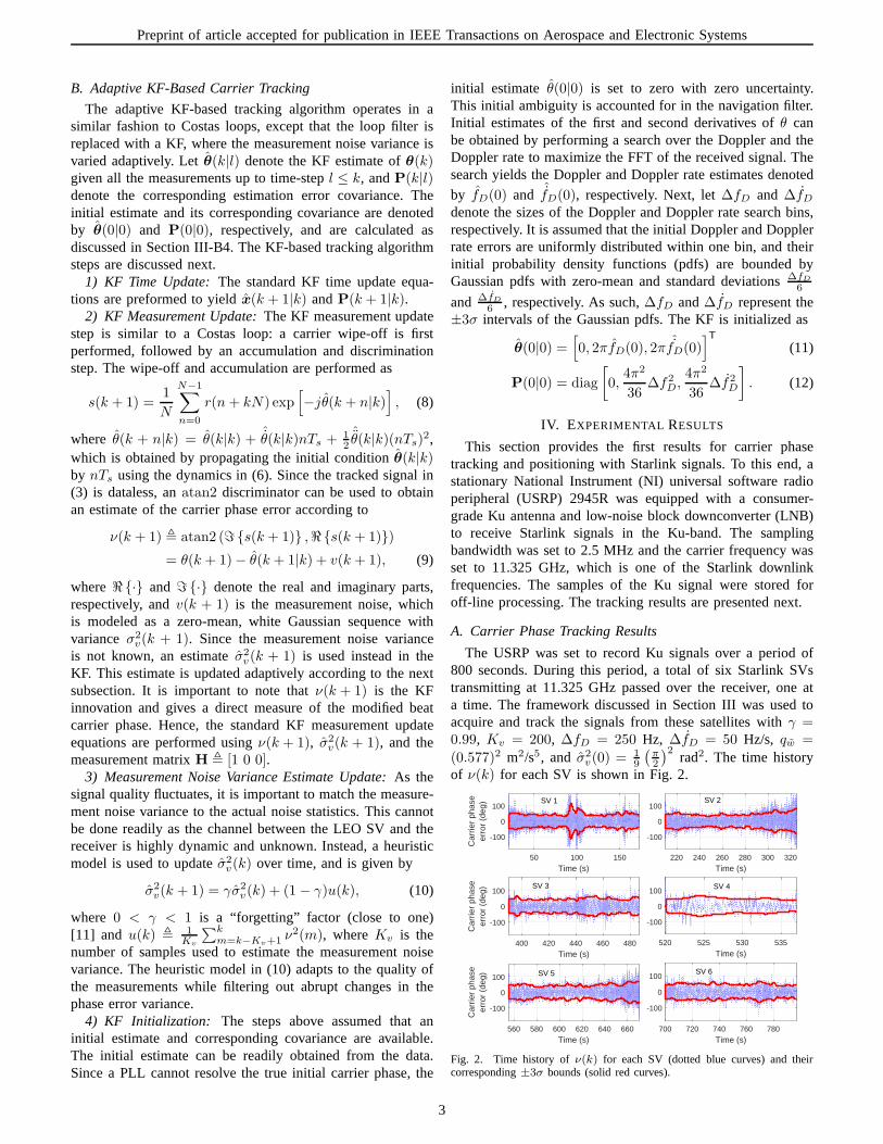
The USRP was set to record Ku signals over a period of800 seconds. During this period, a total of six Starlink SVstransmitting at 11.325 GHz passed over the receiver, one ata time. The framework discussed in Section III was used toacquire and track the signals from these satellites withγ =0.99, Kv = 200, ∆fD = 250 Hz, ∆fD = 50 Hz/s, qw =

(0.577)2 m2/s5, and σ2v(0) = 1

9

(

π2

)2rad2. The time history

of ν(k) for each SV is shown in Fig. 2.

50 100 150

Time (s)

-100

0

100

Car

rier

phas

eer

ror

(deg

)

220 240 260 280 300 320

Time (s)

-100

0

100

400 420 440 460 480

Time (s)

-100

0

100

Car

rier

phas

eer

ror

(deg

)

520 525 530 535

Time (s)

-100

0

100

560 580 600 620 640 660

Time (s)

-100

0

100

Car

rier

phas

eer

ror

(deg

)

700 720 740 760 780

Time (s)

-100

0

100

SV 1 SV 2

SV 3 SV 4

SV 5 SV 6

Fig. 2. Time history ofν(k) for each SV (dotted blue curves) and theircorresponding±3σ bounds (solid red curves).

3

Preprint of article accepted for publication in IEEE Transactions on Aerospace and Electronic Systems

B. Position Solution

Next, carrier phase observables are formed from the trackedmodified beat carrier phases by (i) downsampling by a factorD = 10 to avoid large time-correlations in the carrier phaseobservables and (ii) multiplying by the wavelength to expressthe carrier observable in meters. Leti ∈ {1, 2, 3, 4, 5, 6}denote the SV index. The carrier phase observable to theithSV at time-stepκ = k ·D, expressed in meters, is modeled as

zi(κ)=‖rr−rSVi(κ)‖2+ai κDT+bi+c Ttropo,i(κ)+vzi(κ),

(13)whererr andrSVi

(κ) are the receiver’s andith Starlink SVthree-dimensional (3–D) position vectors expressed in an East-North-Up (ENU) frame centered at the receiver’s true position;ai and bi are the coefficients of the first-order polynomialmodeling the errors due to the initial carrier phase, clockbias, and unknown frequency shiftfp; c is the speed oflight, Ttropo,i(κ) is the tropospheric delay for theith SV; andvzi(κ) is the measurement noise, which is modeled as a zero-mean, white Gaussian random variable with varianceσ2

i (κ).The value ofσ2

i (κ) is nothing but the first diagonal elementof P(κ|κ), expressed in m2. Tropospheric delay estimatesTtropo,i(κ) are obtained using the Hopfield model [12] andsubtracted fromzi(κ) yielding the corrected measurementzi(κ) , zi(κ)− Ttropo,i(κ). Next, define the parameter vector

x ,[

rrT, a1, b1, . . . , a6, b6

]T

. (14)

Let z , [z1(0), z1(1), . . . , z1(K1), . . . , z6(0), z6(1), . . . ,z6(K6)]

T, where Ki denoted the total numberof measurements from theith SV, and let vz ,

[vz1(0), vz1(1), . . . , vz1(K1), . . . , vz6(0), vz6(1), . . . , vz6(K6)]T,

which is a zero-mean Gaussian random vector with a diagonalcovarianceR whose diagonal elements are given byσ2

i (κ).Then, one can readily write the measurement equation

z = g(x) + vz, (15)

whereg(x) is a vector-valued function that maps the param-eter x to the carrier phase observables according to (13).Next, a weighted nonlinear least-squares (WNLS) estimatorwith weight matrixR−1 is solved to obtain an estimate ofx.The SV positions were obtained from TLE files and simplifiedgeneral perturbation 4 (SGP4) software. It is important to notethat the TLE epoch time was adjusted for each SV to accountfor ephemeris errors. This was achieved by minimizing therange residuals for each SV.

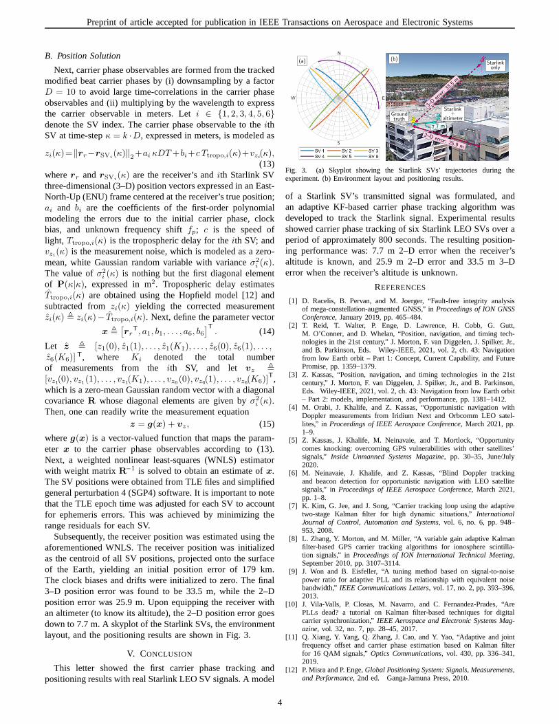
Subsequently, the receiver position was estimated using theaforementioned WNLS. The receiver position was initializedas the centroid of all SV positions, projected onto the surfaceof the Earth, yielding an initial position error of 179 km.The clock biases and drifts were initialized to zero. The final3–D position error was found to be 33.5 m, while the 2–Dposition error was 25.9 m. Upon equipping the receiver withan altimeter (to know its altitude), the 2–D position error goesdown to 7.7 m. A skyplot of the Starlink SVs, the environmentlayout, and the positioning results are shown in Fig. 3.

V. CONCLUSION

This letter showed the first carrier phase tracking andpositioning results with real Starlink LEO SV signals. A model

Starlinkonly

Groundtruth

Starlink+

altimeter

(a) (b)N

S

W E

NE

7.7 m

3{Derror:33.5m

2{D error: 25.9 m

Fig. 3. (a) Skyplot showing the Starlink SVs’ trajectories during theexperiment. (b) Environment layout and positioning results.

of a Starlink SV’s transmitted signal was formulated, andan adaptive KF-based carrier phase tracking algorithm wasdeveloped to track the Starlink signal. Experimental resultsshowed carrier phase tracking of six Starlink LEO SVs over aperiod of approximately 800 seconds. The resulting position-ing performance was: 7.7 m 2–D error when the receiver’saltitude is known, and 25.9 m 2–D error and 33.5 m 3–Derror when the receiver’s altitude is unknown.

REFERENCES

[1] D. Racelis, B. Pervan, and M. Joerger, “Fault-free integrity analysisof mega-constellation-augmented GNSS,” inProceedings of ION GNSSConference, January 2019, pp. 465–484.

[2] T. Reid, T. Walter, P. Enge, D. Lawrence, H. Cobb, G. Gutt,M. O’Conner, and D. Whelan, “Position, navigation, and timing tech-nologies in the 21st century,” J. Morton, F. van Diggelen, J.Spilker, Jr.,and B. Parkinson, Eds. Wiley-IEEE, 2021, vol. 2, ch. 43: Navigationfrom low Earth orbit – Part 1: Concept, Current Capability, and FuturePromise, pp. 1359–1379.

[3] Z. Kassas, “Position, navigation, and timing technologies in the 21stcentury,” J. Morton, F. van Diggelen, J. Spilker, Jr., and B.Parkinson,Eds. Wiley-IEEE, 2021, vol. 2, ch. 43: Navigation from low Earth orbit– Part 2: models, implementation, and performance, pp. 1381–1412.

[4] M. Orabi, J. Khalife, and Z. Kassas, “Opportunistic navigation withDoppler measurements from Iridium Next and Orbcomm LEO satel-lites,” in Proceedings of IEEE Aerospace Conference, March 2021, pp.1–9.

[5] Z. Kassas, J. Khalife, M. Neinavaie, and T. Mortlock, “Opportunitycomes knocking: overcoming GPS vulnerabilities with othersatellites’signals,” Inside Unmanned Systems Magazine, pp. 30–35, June/July2020.

[6] M. Neinavaie, J. Khalife, and Z. Kassas, “Blind Doppler trackingand beacon detection for opportunistic navigation with LEOsatellitesignals,” in Proceedings of IEEE Aerospace Conference, March 2021,pp. 1–8.

[7] K. Kim, G. Jee, and J. Song, “Carrier tracking loop using the adaptivetwo-stage Kalman filter for high dynamic situations,”InternationalJournal of Control, Automation and Systems, vol. 6, no. 6, pp. 948–953, 2008.

[8] L. Zhang, Y. Morton, and M. Miller, “A variable gain adaptive Kalmanfilter-based GPS carrier tracking algorithms for ionosphere scintilla-tion signals,” inProceedings of ION International Technical Meeting,September 2010, pp. 3107–3114.

[9] J. Won and B. Eisfeller, “A tuning method based on signal-to-noisepower ratio for adaptive PLL and its relationship with equivalent noisebandwidth,”IEEE Communications Letters, vol. 17, no. 2, pp. 393–396,2013.

[10] J. Vila-Valls, P. Closas, M. Navarro, and C. Fernandez-Prades, “ArePLLs dead? a tutorial on Kalman filter-based techniques for digitalcarrier synchronization,”IEEE Aerospace and Electronic Systems Mag-azine, vol. 32, no. 7, pp. 28–45, 2017.

[11] Q. Xiang, Y. Yang, Q. Zhang, J. Cao, and Y. Yao, “Adaptiveand jointfrequency offset and carrier phase estimation based on Kalman filterfor 16 QAM signals,”Optics Communications, vol. 430, pp. 336–341,2019.

[12] P. Misra and P. Enge,Global Positioning System: Signals, Measurements,and Performance, 2nd ed. Ganga-Jamuna Press, 2010.

4