Embed Size (px)
Citation preview

Master ThesisMathematical Modeling and SimulationThesis no: 2008 - 6May 2008
Mathematical Modelling of The GlobalPositioning System Tracking Signals
Mounchili Mama
School of EngineeringBlekinge Institute of TechnologySE - 371 79 KarlskronaSweden

This thesis is submitted to the School of Engineering at Blekinge Instituteof Technology in partial fulfillment of the requirements for the degree ofMaster of Science in Mathematical Modeling and Simulation. The thesis is15 credit (15 ECTS ) equivalent to ten weeks of full time studies.
Contact Information
Author : Mounchili MamaE-mail : [email protected]
University advisor : Assistant Professor - Claes JogréusDepartment of Mathematical ScienceEmail : [email protected]
School of EngineeringBlekinge Institute of TechnologySE - 371 79 KarlskronaSweden
Internet : http://www.bth.se/tek/master
Sincere thanks to my Parents andSiblings who always stood by me whenever needed, without whom I couldn’tbe a complete person. Finally to my wife Fatimatou Zahra embellishing mylife, by caring so much about me. I love you Zahra.
Abstract
Recently, there has been increasing interest within the potential user com-munity of Global Positioning System (GPS) for high precision navigationproblems such as aircraft non precision approach, river and harbor navi-gation, real-time or kinematic surveying. In view of more and more GPSapplications, the reliability of GPS is at this issue.
The Global Positioning System (GPS) is a space-based radio navigationsystem that provides consistent positioning, navigation, and timing servicesto civilian users on a continuous worldwide basis. The GPS system receiverprovides exact location and time information for an unlimited number ofusers in all weather, day and night, anywhere in the world.
The work in this thesis will mainly focuss on how to model a Mathematicalexpression for tracking GPS Signal using Phase Locked Loop filter receiver.Mathematical formulation of the filter are of two types: the first orderand the second order loops are tested successively in order to find out acompromised on which one best provide a zero steady state error that willlikely minimize noise bandwidth to tracks frequency modulated signal andreturns the phase comparator characteristic to the null point. Then theZ-transform is used to build a phase-locked loop in software for digitizeddata. Finally, a Numerical Methods approach is developed using eitherMATLAB or Mathematica containing the package for Gaussian eliminationto provide the exact location or the tracking of a GPS in the space for agiven a coarse/acquisition (C/A) code.
i

Acknowledgements
I would like to express my sincere thanks to my supervisor Assistant Pro-fessor - Claes Jogréus for his constructive comments as well as useful advicethroughout the thesis work.
iii
Contents
Contents iv
List of Figures vi
1 Introduction 11.1 Introduction . . . . . . . . . . . . . . . . . . . . . . . . . . . 11.2 GPS Overview . . . . . . . . . . . . . . . . . . . . . . . . . . 11.3 Motivation . . . . . . . . . . . . . . . . . . . . . . . . . . . . 21.4 Scope and Objective . . . . . . . . . . . . . . . . . . . . . . 31.5 Thesis Structure . . . . . . . . . . . . . . . . . . . . . . . . . 3
2 Modeling of GPS Tracking Signals 52.1 GPS Signal Structure . . . . . . . . . . . . . . . . . . . . . . 52.2 Basic Phase-Locked Loops . . . . . . . . . . . . . . . . . . . 7
2.2.1 First-Order Phase-Locked Loop . . . . . . . . . . . . 92.2.2 Second-Order Phase-Locked Loop . . . . . . . . . . . 10
2.3 Z-Transform of Continuous Systems . . . . . . . . . . . . . . 122.4 Carrier and Code Tracking . . . . . . . . . . . . . . . . . . . 132.5 GPS Tarcking Loop Signals . . . . . . . . . . . . . . . . . . 152.6 Conclusion . . . . . . . . . . . . . . . . . . . . . . . . . . . . 16
3 Numerical Method of GPS Tracking Signal 173.1 Introduction . . . . . . . . . . . . . . . . . . . . . . . . . . . 173.2 Numerical Expression of The Coordinates . . . . . . . . . . 183.3 Numerical Solution Using Mathematica . . . . . . . . . . . . 20
4 Global Position Systems Applications 234.1 Introduction . . . . . . . . . . . . . . . . . . . . . . . . . . . 234.2 GPS for The Utilities Industry . . . . . . . . . . . . . . . . . 23
iv

v
4.3 GPS for Civil Engineering Applications . . . . . . . . . . . . 254.4 GPS for Land Seismic Surveying . . . . . . . . . . . . . . . 254.5 GPS for Marine Seismic Surveying . . . . . . . . . . . . . . 274.6 GPS for Vehicle Navigation . . . . . . . . . . . . . . . . . . 294.7 GPS for Transit Systems . . . . . . . . . . . . . . . . . . . 30
Bibliography 33
A GPS Source Code for Data Acquisition 37
List of Figures
1.1 GPS segments . . . . . . . . . . . . . . . . . . . . . . . . . . . . 2
2.1 Architecture of Software-based GPS Receiver . . . . . . . . . . . 62.2 Schematic showing the generation of L1 band GPS signal. The
equation is the mathematical representation of C/A code in L1band . . . . . . . . . . . . . . . . . . . . . . . . . . . . . . . . . 6
2.3 A basic Phase-Locked Loop . . . . . . . . . . . . . . . . . . . . . 82.4 Loop Filter . . . . . . . . . . . . . . . . . . . . . . . . . . . . . 122.5 Code and carrier tracking loops. . . . . . . . . . . . . . . . . . . 14
3.1 Basic idea of GPS positioning . . . . . . . . . . . . . . . . . . . 183.2 Satellite and Observer in the Global Positioning System . . . . . 19
4.1 GPS for utility mapping . . . . . . . . . . . . . . . . . . . . . . 244.2 GPS for construction applications . . . . . . . . . . . . . . . . . 264.3 GPS for land seismic surveying . . . . . . . . . . . . . . . . . . 274.4 GPS for marine seismic surveying . . . . . . . . . . . . . . . . 284.5 GPS for vehicle navigation . . . . . . . . . . . . . . . . . . . . . 294.6 GPS for transit systems . . . . . . . . . . . . . . . . . . . . . . 31
vi

Chapter 1
Introduction
1.1 Introduction
The Global Positioning System (GPS) is a satellite-based navigation system[1], that was developed by the U.S. Department of Defense (DoD) in theearly 1970s. Primarily, GPS was developed as a military system to fulfillU.S. military needs. However, it was later made available to civilians, andis now a dual-use system that can be accessed by both military and civilianusers [2]. GPS provides continuous positioning and timing information,anywhere in the world under any weather conditions. Because it serves anunlimited number of users as well as being used for security reasons, GPSis a one-way-ranging (passive) system [4]. That is, users can only receivethe satellite signals.
1.2 GPS Overview
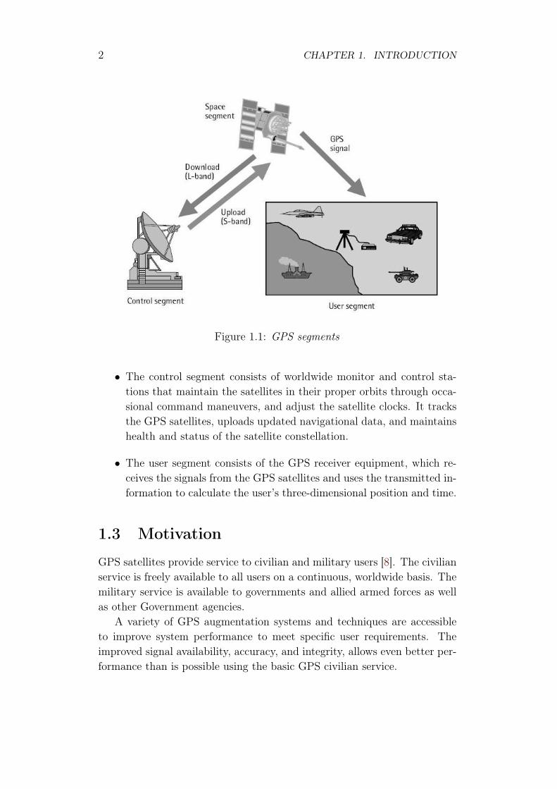
The GPS is made up of three parts: satellites orbiting the Earth; control andmonitoring stations on Earth; and the GPS receivers owned by users. GPSsatellites broadcast signals from space that are picked up and identified byGPS receivers. Each GPS receiver then provides three-dimensional location(latitude, longitude, and altitude) plus the time. Furthermore GPS consistof three segments as shown in Figure 1.1: the space segment, the controlsegment and the user segment.
• The space segment consists of a nominal constellation of 24 operatingsatellites that transmit one-way signals that give the current GPSsatellite position and time.
1
2 CHAPTER 1. INTRODUCTION
Figure 1.1: GPS segments
• The control segment consists of worldwide monitor and control sta-tions that maintain the satellites in their proper orbits through occa-sional command maneuvers, and adjust the satellite clocks. It tracksthe GPS satellites, uploads updated navigational data, and maintainshealth and status of the satellite constellation.
• The user segment consists of the GPS receiver equipment, which re-ceives the signals from the GPS satellites and uses the transmitted in-formation to calculate the user’s three-dimensional position and time.
1.3 Motivation
GPS satellites provide service to civilian and military users [8]. The civilianservice is freely available to all users on a continuous, worldwide basis. Themilitary service is available to governments and allied armed forces as wellas other Government agencies.
A variety of GPS augmentation systems and techniques are accessibleto improve system performance to meet specific user requirements. Theimproved signal availability, accuracy, and integrity, allows even better per-formance than is possible using the basic GPS civilian service.
1.4. SCOPE AND OBJECTIVE 3
The outstanding performance of GPS over many years has earned theconfidence of millions of civil users worldwide. It has proven its dependabil-ity in the past and promises to be of benefit to users, all over the world, farinto the future.
1.4 Scope and Objective
The goal of this thesis work is primarily to formulate some mathematicalmodels that best describe phase locked loop necessary to determine approx-imatively the GPS tracking signal. Then the next step will be to make atransform from continuous to discrete systems to build a phase-locked loopin software for digitized data, the continuous system must be changed intoa discrete system. Numerical method such as the Gaussian Eliminationmethod will be use to simulation on mathematica package the exact posi-tion of a GPS signal receiver in the three dimension space. Finally someGPS applications area will be discussed.
1.5 Thesis Structure
Chapter 1 of the book introduces the GPS system and its components.Chapter 2 examines the mathematical modeling or formulation of GPStracking signal structure, coupled with the GPS modernization, and thekey types of the GPS measurements. Another simple way to determinethe GPS signal is developed using Gaussian Elimination method packageof Mathematical, is presented in Chapter 3. The GPS applications in thevarious fields are given in Chapter 4, which covers the other satellite nav-igation systems developed or proposed in different parts of the world thatfit with different purpose.

Chapter 2
Modeling of GPS Tracking Signals
The main objective in this chapter is to determine how GPS signal canbe processed by using acquisition and tracking algorithms to extract thenavigation information bits from the raw data. The navigation data bitsprovide all the necessary information to compute the pseudo-range betweenthe receiver and the visible satellites.
2.1 GPS Signal Structure
Generally the GPS has two bands, L1 and L2. Where L1 band has coarse /acquisition (C/A) code, P-code and navigation data and L2 band has onlyP-code. The P-code is encrypted with an encryption code and is namedY-code. While the C/A code is a succession of zeros and ones and is uniquefor every satellite. The code is relied on Gold Codes. Two strings of goldcodes with different phase tapings are considered to generate unique C/Acode for each satellite. The C/A code is also called pseudorandom number(PRN) code. PRN code or number is attributed to every satellite dependingon which PRN code is attributed to a particular satellite. If PRN (C/A)code of 1 is assigned to a satellite, in that case this satellite is named asPRN-1. The particularities of C/A codes are that they have the best cross-correlation feature. The cross-correlation among any two codes is muchlower than auto-correlation of each one of the codes. The frequency of theC/A code is 1.023 MHz. P-code is also a sequence of zeros and ones and isgenerated using a set of Gold Codes. P-code has a frequency of 10.23 MHz.
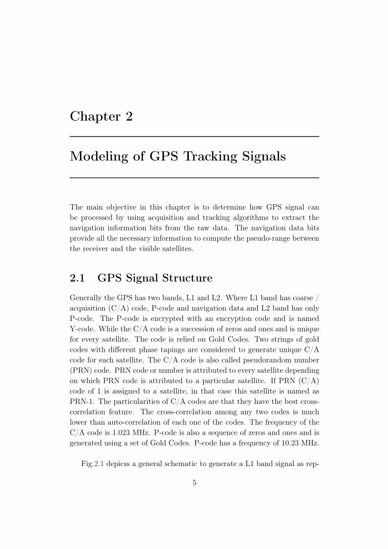
Fig.2.1 depicss a general schematic to generate a L1 band signal as rep-
5
6 CHAPTER 2. MODELING OF GPS TRACKING SIGNALS
Figure 2.1: Architecture of Software-based GPS Receiver
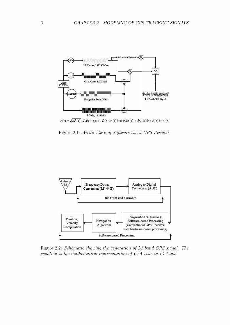
Figure 2.2: Schematic showing the generation of L1 band GPS signal. Theequation is the mathematical representation of C/A code in L1 band
2.2. BASIC PHASE-LOCKED LOOPS 7
resented by the equation shown in the figure for C/A code. In conventionalhardware-based GPS receiver, the lower three blocks in Fig.2.2 are imple-mented in an IC chip and hence the user cannot access the algorithmsbuilt inside the chips. In software-based receiver, these blocks are fullyimplemented using high level programming languages granting the user acomplete control over the algorithms. Hence the main difference betweenthe software-based GPS receiver and a conventional hardware receiver.
2.2 Basic Phase-Locked Loops
During the tracking process, the center frequency of the narrow-band filteris fixed, while a locally generated signal follows the frequency of the inputsignal. Moreover the phases of both signals are compared through a phasecomparator of which passes through a narrow-band filter. Given that thetracking circuit posses narrow bandwidth, the sensitivity is fairly high incomparison with the acquisition method.
In the case of phase shifts in the carrier due to the C/A code, as in a GPSsignal, the code has to be stripped off first. The tracking process will followthe signal and acquire the information of the navigation data. In case aGPS receiver is stationary, the desired frequency variation is very slow dueto satellite motion. Given this condition, the frequency variation of thelocally generated signal is also slow; consequently, the update rate of thetracking loop can be low. Therefore, to track a GPS signal two trackingloops are needed: a loop to track the carrier frequency referred as carrierloop and the other one to track the C/A code known as the code loop.
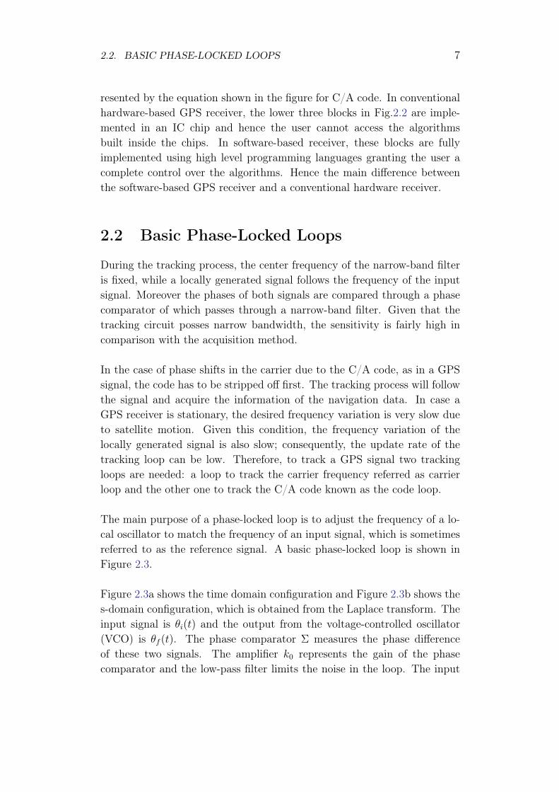
The main purpose of a phase-locked loop is to adjust the frequency of a lo-cal oscillator to match the frequency of an input signal, which is sometimesreferred to as the reference signal. A basic phase-locked loop is shown inFigure 2.3.
Figure 2.3a shows the time domain configuration and Figure 2.3b shows thes-domain configuration, which is obtained from the Laplace transform. Theinput signal is θi(t) and the output from the voltage-controlled oscillator(VCO) is θf (t). The phase comparator Σ measures the phase differenceof these two signals. The amplifier k0 represents the gain of the phasecomparator and the low-pass filter limits the noise in the loop. The input
8 CHAPTER 2. MODELING OF GPS TRACKING SIGNALS
Figure 2.3: A basic Phase-Locked Loop
voltage Vo to the VCO controls its output frequency, which can be expressedas:
ω2(t) = ω0 + k1u(t) (2.1)
where ω0 is the center angular frequency of the VCO, k1 is the gain ofthe VCO, and u(t) is a unit step function, which is defined as [6]:
u(t) =
{0 for t < 0
1 for t > 0(2.2)
The phase angle of the VCO can be obtained by integrating Equation (2.1)as: ∫ t
0
ω2(t)dt = ω0t+ θf (t) = ω0t+
∫ t
0
k1u(t)dt
Where:
θf (t) =
∫ t
0
k1u(t)dt (2.3)
The Laplace transform [7] of θf (t) is:
θf (s) =k1
s(2.4)
We can obtain from the Figure 2.1b the following equations:
Vc(s) = k0ε(s) = k0[θi(s)− θf (s)] (2.5)
V0(s) = Vc(s)F (s) (2.6)
θf (s) = V0(s)k1
s(2.7)
Hence result the following:
ε(t) = θi(s)− θf (s) =Vc(s)
k0
=V0(s)
k0F (s)=
sθf (s)
k0k1F (s)or
2.2. BASIC PHASE-LOCKED LOOPS 9
θi(s) = θf (s)
(1 +
s
k0k1F (s)
)(2.8)
Where ε(s) is the error function. The transfer function H(s) of the loop isdefined as:
H(s) ≡ θf (s)
θi(s)=
k0k1F (s)
s+ k0k1F (s)(2.9)
The error transfer function can be defined as:
He(s) =ε(s)
θi(s)=θi(s)− θf (s)
θi(s)= 1−H(s) =
s
s+ k0k1F (s)(2.10)
The equivalent noise bandwidth is defined as:
Bn =
∫ ∞0
|H(jω)|2df (2.11)
Where ω is the angular frequency and is related to the frequency f byω = 2πf
In order to study the properties of the phase-locked loops, two types ofinput signals are usually studied. The first type is a unit step function as:
θi(t) = u(t) or θi(s) =1
s(2.12)
The second type is a frequency-modulated signal
θi(t) = ∆ω(t) or θi(s) =∆ω
s2(2.13)
2.2.1 First-Order Phase-Locked Loop
A first-order phase-locked loop implies that the denominator of the transferfunction H(s) is a first-order function of s [6]. The order of the phase-lockedloop depends on the order of the filter in the loop. The expression of thefilter function in the case of the first order phase-locked loop, is:
F (s) = 1 (2.14)
Hence the simplest expression of phase-locked loop. In the case of a unitstep function input, the equivalent transfer function from Equation (2.9)becomes:
10 CHAPTER 2. MODELING OF GPS TRACKING SIGNALS
H(s) =k0k1
s+ k0k1
(2.15)
Then the noise bandwidth can be expressed as:
Bn =
∫ ∞0
(k0k1)2
ω2 + (k0k1)2df =
(k0k1)2
2π
∫ ∞0
dω
ω2 + (k0k1)2
Bn =(k0k1)
2
2πk0k1
tan−1
(ω
k0k1
)∞0
=k0k1
4(2.16)
Given the input signal θi(s) = 1/s, the error function can be found fromEquation (2.10) as:
ε(s) = θi(s)He(s)1
s+ k0k1
(2.17)
The steady-state error can be found from the final value theorem [7] of theLaplace transform as follow:
limt→∞
y(t) = lims→0
sY (s) (2.18)
It follows from this relation, the final value of ε(t) can be found as:
limt→∞
ε(t) = lims→0
sε(s) = lims→0
s
s+ k0k1
= 0 (2.19)
Given the input signal θi(s) = ∆ω/s2, the error function becomes:
ε(s) = θi(s)He(s)∆ω
s
1
s+ k0k1
(2.20)
Then the steady state error becomes:
limt→0
ε(t) = lims→0
sε(s) = lims→0
∆ω
s+ k0k1
=∆ω
k0k1
(2.21)
It results that the steady-state phase error is not equal to zero. Thereforefor a large value of k0k1 makes the error small. However, from Equation(2.15) the 3 dB bandwidth occurs at s = k0k1. Thus a small value of ε(t)also means large bandwidth, that is likely to contain more noise.
2.2.2 Second-Order Phase-Locked Loop
In the case of a second-order phase-locked loop means the denominator ofthe transfer function H(s) is a second-order function of s. One of the filters
2.2. BASIC PHASE-LOCKED LOOPS 11
to make such a second-order phase-locked loop is
F (s) =sτ2 + 1
sτ1(2.22)
Replacing this relation into Equation (2.9), the transfer function becomes:
H(s) =k0k1τ2sτ1
+ k0k1τ1
s2 k0k1τ2sτ1
+ k0k1τ1
≡ 2ζωns+ ω2n
s2 + 2ζωns+ ω2n
(2.23)
where ωn is the natural frequency, which can be expressed as:
ωn =
√k0k1
τ1(2.24)
and ζ the damping factor which can be determined as follow:
2ζωn =k0k1τ2τ1
or ζ =ωnτ2
2(2.25)
Therefore the noise bandwidth can be found as:
Bn =
∫ ∞0
|H(jω)|2df =ωn2π
∫ ∞0
1 +(
2ζ ωωn
)2
[1−
(ωωn
)2]2
+(
2ζ ωωn
)2dw
or
=ωn2π
∫ ∞0
1 + 4ζ2(ωωn
)2
(ωωn
)4
+ 2(2ζ2 − 1)(ωωn
)2
+ 1dw =
ωn2
(ζ +
1
4ζ
)(2.26)
This integration can be found in the appendix of [6]. Therefore the errortransfer function can be obtained from Equation (2.10) as:
He(s) = 1−H(s) =s2
s2 + 2ζωns+ ω2n
(2.27)
And whenever θi(s) = 1/s, the error function becomes:
ε(s) =s2
s2 + 2ζωns+ ω2n
(2.28)
At steady state the error is given by:
limt→∞
ε(t) = lims→0
sε(s) = 0 (2.29)
12 CHAPTER 2. MODELING OF GPS TRACKING SIGNALS
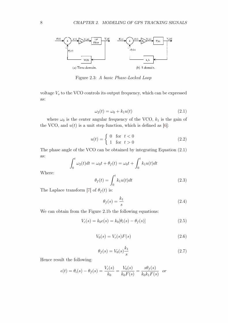
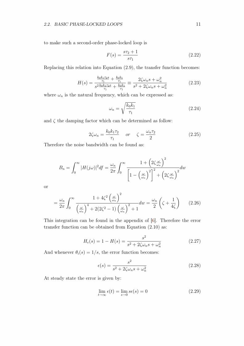
Figure 2.4: Loop Filter
Unlike the first-order loop, the steady-state error is zero for the frequencymodulated signal. Meaning that, the second-order loop tracks a frequency-modulated signal and returns the phase comparator characteristic to thenull point. Therefore, the conventional phase-locked loop in a GPS receiveris usually a second-order one.
2.3 Z-Transform of Continuous Systems
In order to build a phase-locked loop in software for digitized data, thecontinuous system must be changed into a discrete system. The transferfrom the continuous s-domain into the discrete z-domain is through bilineartransform as:
s =2
ts
1− z−1
1 + z−1(2.30)
where ts is the sampling interval. Substituting this relation in Equation(2.22) the filter is transformed to:
F (z) = C1 +C2
1− z−1=
(C1 + C2)− C1z−1
1− z−1(2.31)
where:
C1 =2τ2 − ts
2τ1and C2 =
tsτ1
(2.32)
This filter is shown in Figure 2.4. The VCO in the phase-locked loop isreplaced by a direct digital frequency synthesizer and its transfer functionN(z) can be used to replace the result in Equation (2.7) with:
2.4. CARRIER AND CODE TRACKING 13
N(z) =θf (z)
V0(z)≡ k1z
−1
1− z−1(2.33)
Using the same approach as Equation (2.8), the transfer function H(z) canbe written as:
H(z) =θf (z)
θi(z)=
k0F (z)N(z)
1 + k0F (z)N(z)(2.34)
The substituting the results of Equations (2.33) and (2.35) into the aboveequation, yields:
H(z) =k0k1(C1 + C2)z
−1 − k0k1C1z−2
1 + [k0k1(C1 + C2)− 2]z−1 + (1− k0k1C1)z−2(2.35)
By using the bilinear transform in Equation (2.32) to Equation (2.23), theresult can be written as:
H(z) =[4ζωn + (ωnts)
2] + 2(ωnts)2z−1 + [(ωnts)
2 − rζωnts]z−2
[4 + 4ζωn + (ωnts)2] + [2(ωnts)2 − 8]z−1 + [4− 4ζωn + (ωnts)2]z−2
(2.36)By equating the denominator polynomials in the above two equations, C1
and C2 can be determined as:
C1 =1
k0k1
8ζωnts4 + 4ζωnts + (ωnts)2
C2 =1
k0k1
4ζωnts4 + 4ζωnts + (ωnts)2
(2.37)
The filter here is implemented in digital format and the result can be used forphase-locked loop designs, but it is not the part of this thesis scope since weare only concerned with mathematical expression. Where the desired noisebandwidth signal from the Equation (2.26) can is expressed as:
Bn =ωn2
(ζ +
1
4ζ
)
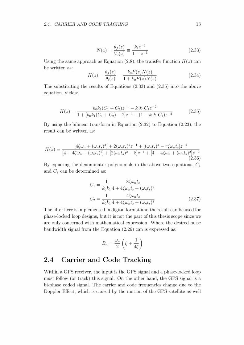
2.4 Carrier and Code Tracking
Within a GPS receiver, the input is the GPS signal and a phase-locked loopmust follow (or track) this signal. On the other hand, the GPS signal is abi-phase coded signal. The carrier and code frequencies change due to theDoppler Effect, which is caused by the motion of the GPS satellite as well

14 CHAPTER 2. MODELING OF GPS TRACKING SIGNALS
Figure 2.5: Code and carrier tracking loops.
as from the motion of the GPS receiver. In order to track the GPS signal,the C/A code information have to be removed. Consequently, it requirestwo phase-locked loops to track a GPS signal. One loop is to track the C/A code and the other one is to track the carrier frequency. These two loopsmust be coupled together are depicted in Figure 3.3.
In Figure 2.3, the C/A code loop generates three outputs: an earlycode, a late code, and a prompt code. The prompt code is applied to thedigitized input signal and strips the C/A code from the input signal. Strip-ping the C/A code means to multiply the C/A code to the input signalwith the proper phase. The output will be a continuous wave (cw) signalwith phase transition caused only by the navigation data. This signal isapplied to the input of the carrier loop. The output from the carrier loopis a cw with the carrier frequency of the input signal. This signal is usedto strip the carrier from the digitized input signal, which means using thissignal to multiply the input signal. The output is a signal with only a C/Acode and no carrier frequency, which is applied to the input of the code loop.
Every output passes through a moving average filter and the output ofthe filter is squared. The two squared outputs are compared to generate a
2.5. GPS TARCKING LOOP SIGNALS 15
control signal to adjust the rate of the locally generated C/A code to matchthe C/A code of the input signal. The locally generated C/A code is theprompt C/A code and this signal is used to strip the C/A code from thedigitized input signal.
The carrier frequency loop receives a cw signal phase modulated onlyby the navigation data as the C/A code is stripped off from the input sig-nal. The acquisition program determines the initial value of the carrierfrequency. The voltage-controlled oscillator (VCO) generates a carrier fre-quency with respect to the value obtained from the acquisition program.This signal is divided into two paths: a direct path and the other one witha 90-degree phase shift. These two signals are correlated with the inputsignal. The outputs of the correlators are filtered and their phases are com-pared against each other through an arctangent comparator.
The arctangent process is insensitive to the phase transition caused bythe navigation data and it can be considered as one type of a Costas loop.A Costas loop is a phase-locked loop, which is insensitive to phase transi-tion. The output of the comparator is filtered again and generates a controlsignal. This control signal is used to tune the oscillator to generate a carrierfrequency to follow the input cw signal. This carrier frequency is also usedto strip the carrier from the input signal.
2.5 GPS Tarcking Loop Signals
The input data to the tracking loop are collected from satellites. Severalconstants have to be determined such as the noise bandwidth, the gain fac-tors of the phase detector, and the VCO (or the digital frequency synthe-sizer). These constants are determined through trial and error or guessingand are by no means optimized. This tracking program is applied only onlimited data length. Although it generates acceptable results, further studymight be needed if it is used in a software GPS receiver designed to tracklong records of data. The following steps can be applied to both the codeloop and the carrier loop:
1. Set the bandwidths and the gain of the code and carrier loops. Theloop gain includes the gains of the phase detector and the VCO. Thebandwidth of the code loop is narrower than the carrier loop becauseit tracks the signal for a longer period of time. Select the noise band-
16 CHAPTER 2. MODELING OF GPS TRACKING SIGNALS
width of the code loop to be 1 Hz and the carrier loop to be 20 Hz.This is one set of several probable selections that the tracking programcan run.
2. Choose the damping factor in Equation (2.25) to be ζ = .707. The ζvalue is often assumed near about its optimum [9].
3. The natural frequency can be found from Equation (2.26).
4. Select the code loop gain (k0k1) to be 50 and the carrier loop gain tobe 4π100. These values are also one set of several possible selections.The constants C1 and C2 of the filter can be found from Equation(2.39).
The above four steps provide the necessary information for the two loops.Once the constants of the loops are known, the phase of the code loop andthe phase of the carrier frequency can be adjusted to follow the input signals.
2.6 Conclusion
Hence the completed the algorithms for acquisition and tracking. The goalof these algorithms has to be tested on various data sets in different envi-ronment using different type of antenna including left hand and right handpolarized antenna. I have found that, it is necessary to tune the parametersof the tracking algorithm and threshold values of acquisition either dynam-ically or based on some rule for successful acquisition and tracking of GPSsignal in standard environment. In some cases, we have found that trackingcould not be done for satellites though acquisition is perfect. In this case,a change of parameter values of the Phase Lock Loop manually makes thetracking successful. This type of manual setting shall be automated in thefuture. The future work consists of extracting the navigation message fromthe tracking output and to compute the position of the receiver. It is alsonecessary to make the processing as fast as possible.
Chapter 3
Numerical Method of GPS TrackingSignal
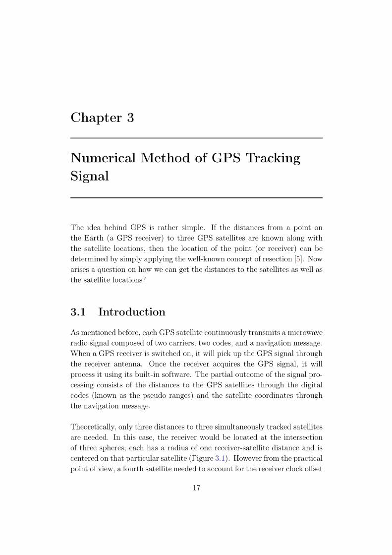
The idea behind GPS is rather simple. If the distances from a point onthe Earth (a GPS receiver) to three GPS satellites are known along withthe satellite locations, then the location of the point (or receiver) can bedetermined by simply applying the well-known concept of resection [5]. Nowarises a question on how we can get the distances to the satellites as well asthe satellite locations?
3.1 Introduction
As mentioned before, each GPS satellite continuously transmits a microwaveradio signal composed of two carriers, two codes, and a navigation message.When a GPS receiver is switched on, it will pick up the GPS signal throughthe receiver antenna. Once the receiver acquires the GPS signal, it willprocess it using its built-in software. The partial outcome of the signal pro-cessing consists of the distances to the GPS satellites through the digitalcodes (known as the pseudo ranges) and the satellite coordinates throughthe navigation message.
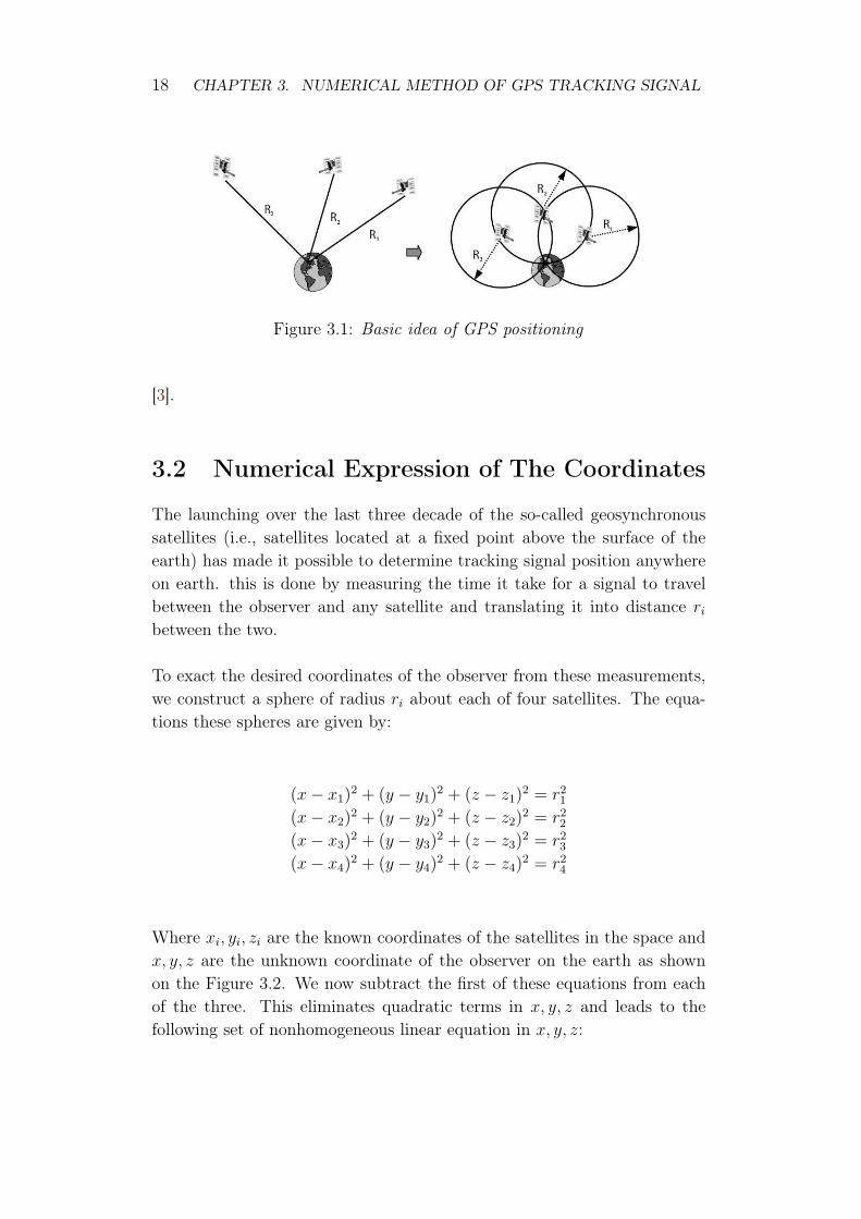
Theoretically, only three distances to three simultaneously tracked satellitesare needed. In this case, the receiver would be located at the intersectionof three spheres; each has a radius of one receiver-satellite distance and iscentered on that particular satellite (Figure 3.1). However from the practicalpoint of view, a fourth satellite needed to account for the receiver clock offset
17
18 CHAPTER 3. NUMERICAL METHOD OF GPS TRACKING SIGNAL
Figure 3.1: Basic idea of GPS positioning
[3].
3.2 Numerical Expression of The Coordinates
The launching over the last three decade of the so-called geosynchronoussatellites (i.e., satellites located at a fixed point above the surface of theearth) has made it possible to determine tracking signal position anywhereon earth. this is done by measuring the time it take for a signal to travelbetween the observer and any satellite and translating it into distance ribetween the two.
To exact the desired coordinates of the observer from these measurements,we construct a sphere of radius ri about each of four satellites. The equa-tions these spheres are given by:
(x− x1)2 + (y − y1)
2 + (z − z1)2 = r2
1
(x− x2)2 + (y − y2)
2 + (z − z2)2 = r2
2
(x− x3)2 + (y − y3)
2 + (z − z3)2 = r2
3
(x− x4)2 + (y − y4)
2 + (z − z4)2 = r2
4
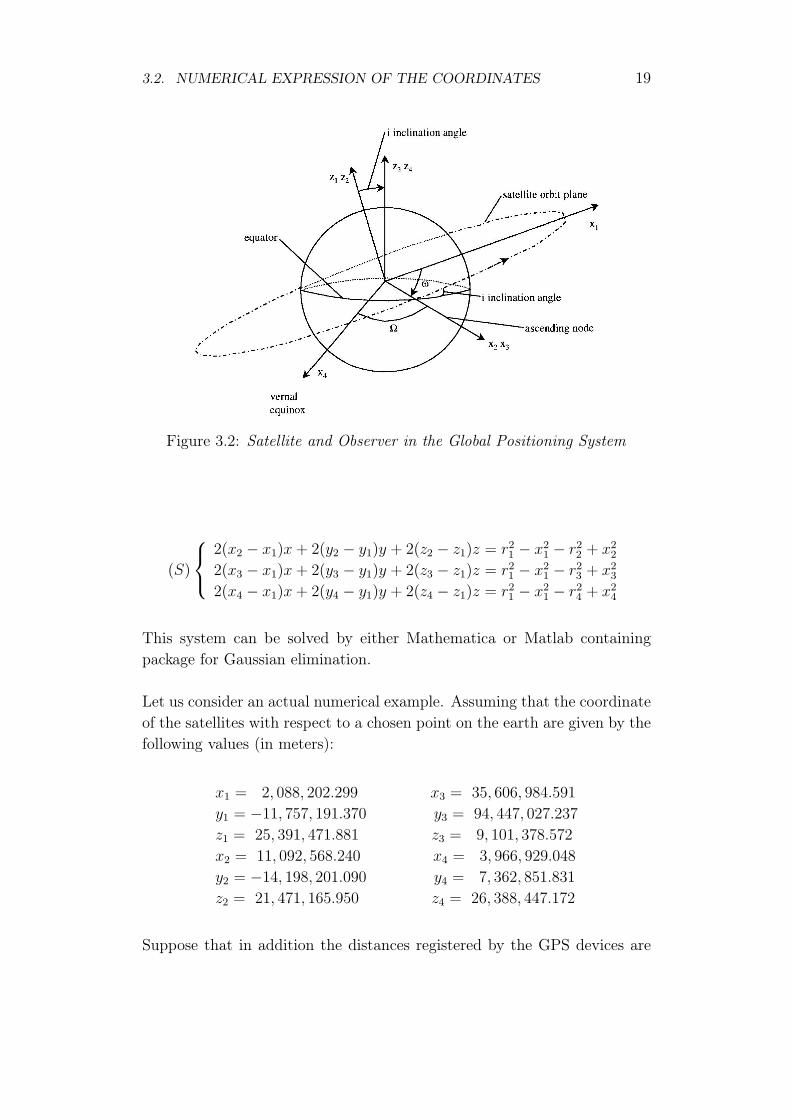
Where xi, yi, zi are the known coordinates of the satellites in the space andx, y, z are the unknown coordinate of the observer on the earth as shownon the Figure 3.2. We now subtract the first of these equations from eachof the three. This eliminates quadratic terms in x, y, z and leads to thefollowing set of nonhomogeneous linear equation in x, y, z:
3.2. NUMERICAL EXPRESSION OF THE COORDINATES 19
Figure 3.2: Satellite and Observer in the Global Positioning System
(S)
2(x2 − x1)x+ 2(y2 − y1)y + 2(z2 − z1)z = r2
1 − x21 − r2
2 + x22
2(x3 − x1)x+ 2(y3 − y1)y + 2(z3 − z1)z = r21 − x2
1 − r23 + x2
3
2(x4 − x1)x+ 2(y4 − y1)y + 2(z4 − z1)z = r21 − x2
1 − r24 + x2
4
This system can be solved by either Mathematica or Matlab containingpackage for Gaussian elimination.
Let us consider an actual numerical example. Assuming that the coordinateof the satellites with respect to a chosen point on the earth are given by thefollowing values (in meters):
x1 = 2, 088, 202.299 x3 = 35, 606, 984.591
y1 = −11, 757, 191.370 y3 = 94, 447, 027.237
z1 = 25, 391, 471.881 z3 = 9, 101, 378.572
x2 = 11, 092, 568.240 x4 = 3, 966, 929.048
y2 = −14, 198, 201.090 y4 = 7, 362, 851.831
z2 = 21, 471, 165.950 z4 = 26, 388, 447.172
Suppose that in addition the distances registered by the GPS devices are
20 CHAPTER 3. NUMERICAL METHOD OF GPS TRACKING SIGNAL
given by:r1 = 23, 204, 698.51
r2 = 21, 585, 835, 37
r3 = 31, 364, 260.01
r4 = 24, 966, 798.73
Using the Gaussian Elimination to solve the system (S), the following resultsare obtained:
x = −3.0168 ∗ 106m
y = 7231.03m
z = −3.13188 ∗ 107m
These are the coordinates of the observer with respect to a fixed knownorigin on earth. Hence we have here the application of simple expressionsdrawn from the analytical geometry of sphere and the elementary use ofGaussian elimination to arrive at the solution of a problem of some so-phistication. The practical implementation of the GPS had to await thedeployment of geosynchronous satellite and the hardware needed to pro-duce compact GPS devices, which can now be installed in automobiles.
It is worth mentioning here that three equation (i.e., the use of only threesatellites in our case given that many can be involved) would have been suffi-cient to calculate the coordinates x, y, z of the observer. In practice problemwhen many satellites come into play. Hence the need to develop computeralgorithm that could be used to solve the problem in such situation.
3.3 Numerical Solution Using Mathematica
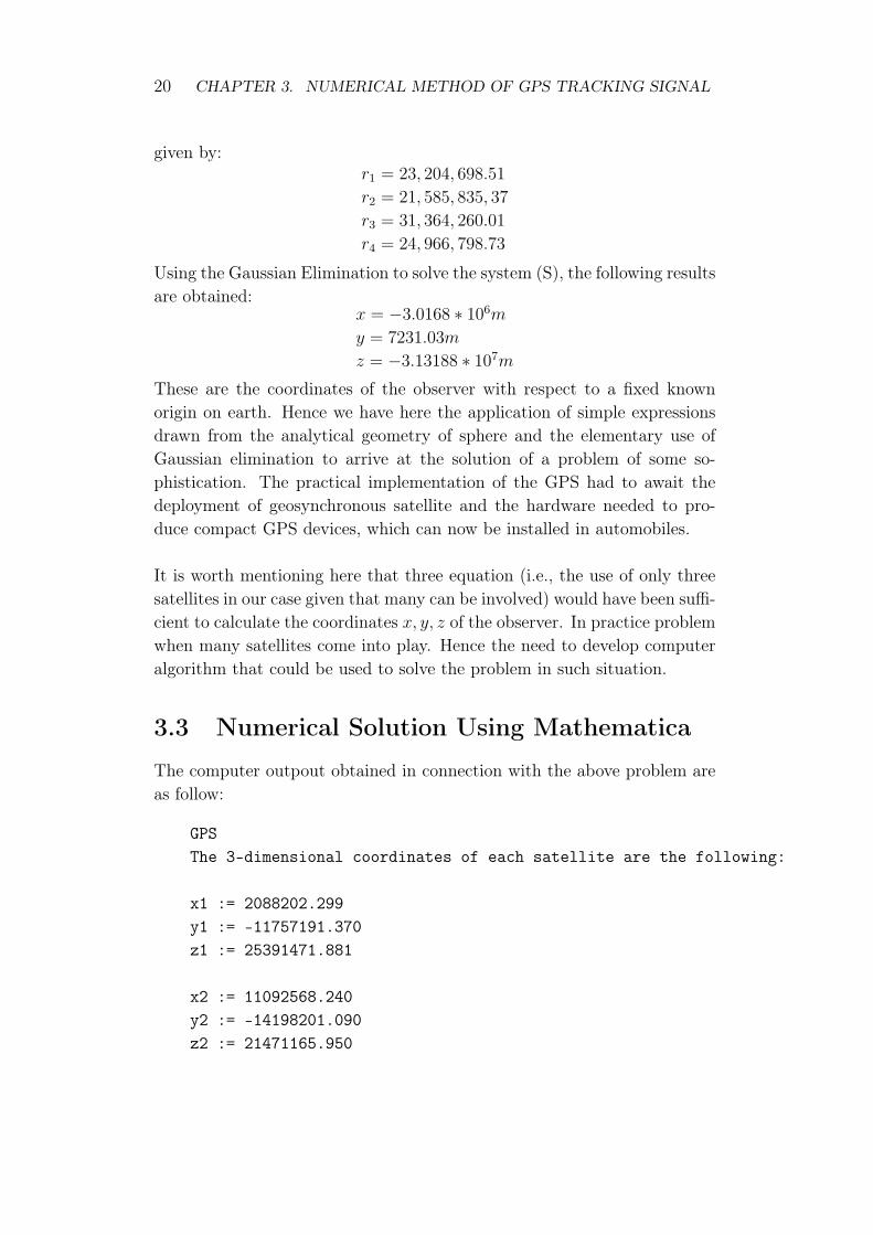
The computer outpout obtained in connection with the above problem areas follow:
GPSThe 3-dimensional coordinates of each satellite are the following:
x1 := 2088202.299y1 := -11757191.370z1 := 25391471.881
x2 := 11092568.240y2 := -14198201.090z2 := 21471165.950
3.3. NUMERICAL SOLUTION USING MATHEMATICA 21
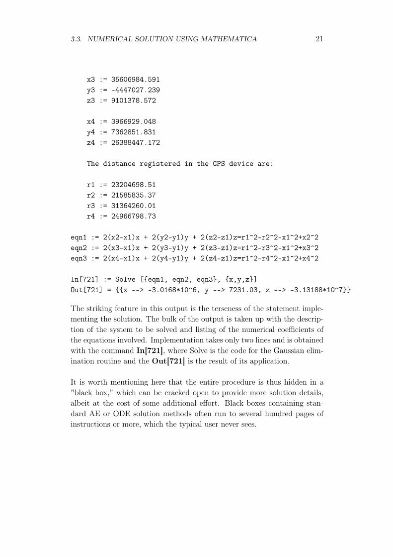
x3 := 35606984.591y3 := -4447027.239z3 := 9101378.572
x4 := 3966929.048y4 := 7362851.831z4 := 26388447.172
The distance registered in the GPS device are:
r1 := 23204698.51r2 := 21585835.37r3 := 31364260.01r4 := 24966798.73
eqn1 := 2(x2-x1)x + 2(y2-y1)y + 2(z2-z1)z=r1^2-r2^2-x1^2+x2^2eqn2 := 2(x3-x1)x + 2(y3-y1)y + 2(z3-z1)z=r1^2-r3^2-x1^2+x3^2eqn3 := 2(x4-x1)x + 2(y4-y1)y + 2(z4-z1)z=r1^2-r4^2-x1^2+x4^2
In[721] := Solve [{eqn1, eqn2, eqn3}, {x,y,z}]Out[721] = {{x --> -3.0168*10^6, y --> 7231.03, z --> -3.13188*10^7}}
The striking feature in this output is the terseness of the statement imple-menting the solution. The bulk of the output is taken up with the descrip-tion of the system to be solved and listing of the numerical coefficients ofthe equations involved. Implementation takes only two lines and is obtainedwith the command In[721], where Solve is the code for the Gaussian elim-ination routine and the Out[721] is the result of its application.
It is worth mentioning here that the entire procedure is thus hidden in a"black box," which can be cracked open to provide more solution details,albeit at the cost of some additional effort. Black boxes containing stan-dard AE or ODE solution methods often run to several hundred pages ofinstructions or more, which the typical user never sees.


Chapter 4
Global Position Systems Applications
GPS has found his way into many applications, mainly as result of its ac-curacy, global availability, and cost-effectiveness.
4.1 Introduction
GPS has been available for civil and military use for more than two decades.That period of time has witnessed the creation of numerous new GPS ap-plications. Because it provides high-accuracy positioning in a cost effectivemanner, GPS has found its way into many industrial applications, replacingconventional methods in most cases. For example, with GPS, machineriescan be automatically guided and controlled. This is especially useful inhazardous areas, where human lives are endangered. Even some species ofbirds are benefiting from GPS technology, as they are being monitored withGPS during their immigration season. This way, help can be presented asneeded. This chapter describes how GPS is being used in land, marine, andairborne applications.
4.2 GPS for The Utilities Industry
Accurate and up-to-date maps of utilities are essential for utility companies.The availability of such maps helps electric, gas, and water utility compa-nies to plan, build, and maintain their assets.
The GPS/GIS system provides a cost-effective, efficient, and accuratetool for creating utility maps. With the help of GPS, locations of features
23
24 CHAPTER 4. GLOBAL POSITION SYSTEMS APPLICATIONS
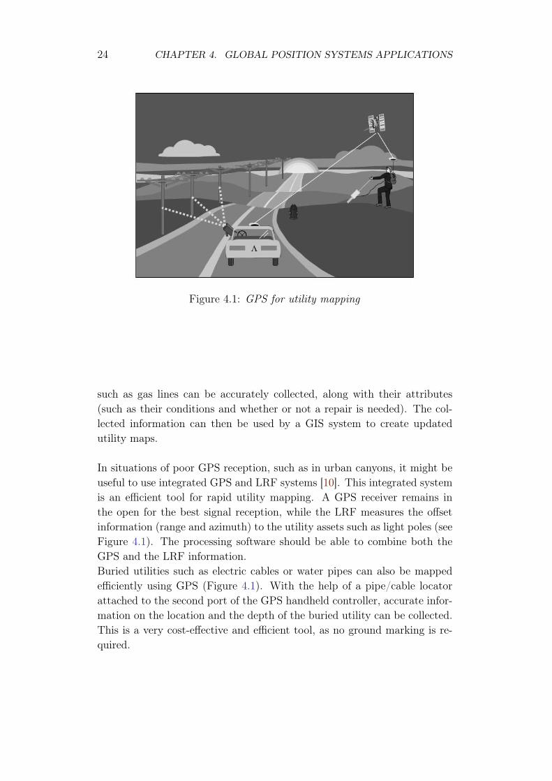
Figure 4.1: GPS for utility mapping
such as gas lines can be accurately collected, along with their attributes(such as their conditions and whether or not a repair is needed). The col-lected information can then be used by a GIS system to create updatedutility maps.
In situations of poor GPS reception, such as in urban canyons, it might beuseful to use integrated GPS and LRF systems [10]. This integrated systemis an efficient tool for rapid utility mapping. A GPS receiver remains inthe open for the best signal reception, while the LRF measures the offsetinformation (range and azimuth) to the utility assets such as light poles (seeFigure 4.1). The processing software should be able to combine both theGPS and the LRF information.Buried utilities such as electric cables or water pipes can also be mappedefficiently using GPS (Figure 4.1). With the help of a pipe/cable locatorattached to the second port of the GPS handheld controller, accurate infor-mation on the location and the depth of the buried utility can be collected.This is a very cost-effective and efficient tool, as no ground marking is re-quired.
4.3. GPS FOR CIVIL ENGINEERING APPLICATIONS 25
4.3 GPS for Civil Engineering Applications
Civil engineering works are often done in a complex and unfriendly envi-ronment, making it difficult for personnel to operate efficiently. The abilityof GPS to provide real-time submeter- and centimeter-level accuracy in acost-effective manner has significantly changed the civil engineering indus-try. Construction firms are using GPS in many applications such as roadconstruction, Earth moving, and fleet management.
In road construction and Earth moving, GPS, combined with wireless com-munication and computer systems, is installed onboard the Earthmovingmachine [11]. Designed surface information, in a digital format, is uploadedinto the system. With the help of the computer display and the real-timeGPS position information, the operator can view whether the correct gradehas been reached (see Figure 4.2). In situations in which millimeter-levelelevation is needed, GPS can be integrated with rotated beam lasers [12].
The same technology (i.e.) combined GPS, wireless communications,and computers) is also used for foundation works (e.g., pile positioning)and precise structural placement (e.g., prefabricated bridge sections andcoastal structures). In these applications, the operators are guided throughthe onboard computer displays, eliminating the need for conventional meth-ods [13].
GPS is also used to track the location and usage of equipment at differ-ent sites. By sending this information to a central location, GPS enablescontractors to deploy their equipment more efficiently. Moreover, vehicleoperators can be efficiently guided to their destinations
4.4 GPS for Land Seismic Surveying
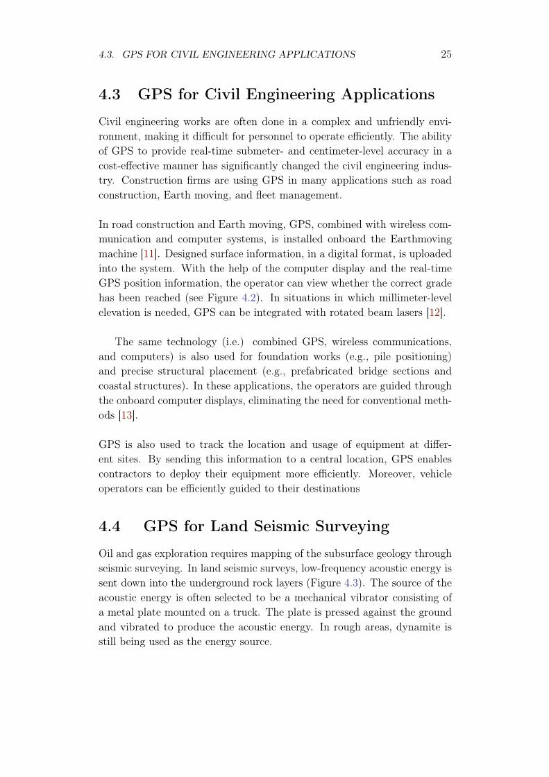
Oil and gas exploration requires mapping of the subsurface geology throughseismic surveying. In land seismic surveys, low-frequency acoustic energy issent down into the underground rock layers (Figure 4.3). The source of theacoustic energy is often selected to be a mechanical vibrator consisting ofa metal plate mounted on a truck. The plate is pressed against the groundand vibrated to produce the acoustic energy. In rough areas, dynamite isstill being used as the energy source.

26 CHAPTER 4. GLOBAL POSITION SYSTEMS APPLICATIONS
Figure 4.2: GPS for construction applications
As the acoustic energy (signal) crosses the various underground rocklayers, it is affected by the physical properties of the rocks. Portions of thesignal are reflected back to the surface by the various layers. The reflectedenergy can be detected by special seismic devices called geophones, whichare laid out al known distances from the energy Source along the survey line(Figure 4.3). Upon detecting .seismic energy, geophones output electricalsignals that are proportional to the intensity of the reflected energy [14].The electrical signals are then recorded on magnetic tapes for geophysicalanalysis and interpretation.
It is clear that unless the positions of the energy source and the geophonesare known with sufficient accuracy, the very expensive seismic data becomesuseless. GPS is used to provide the positioning information in a standard
4.5. GPS FOR MARINE SEISMIC SURVEYING 27
Figure 4.3: GPS for land seismic surveying
or a user-defined coordinate system. Integrated GPS/GLONASS (GlobalNavigation Satellite System) and GPS/digital barometer systems have beenused successfully in situations of poor GPS signal reception [15]. With thehelp of GPS, the environmental impacts (e.g., the need to cut trees) as wellas the operating cost of seismic surveys have been reduced significantly.
4.5 GPS for Marine Seismic Surveying
Marine seismic surveying is similar in principle to land seismic surveying.That is, a low-frequency acoustic energy is sent down into the subsurfacerock layers, and is reflected back to the surface to reveal information about
28 CHAPTER 4. GLOBAL POSITION SYSTEMS APPLICATIONS
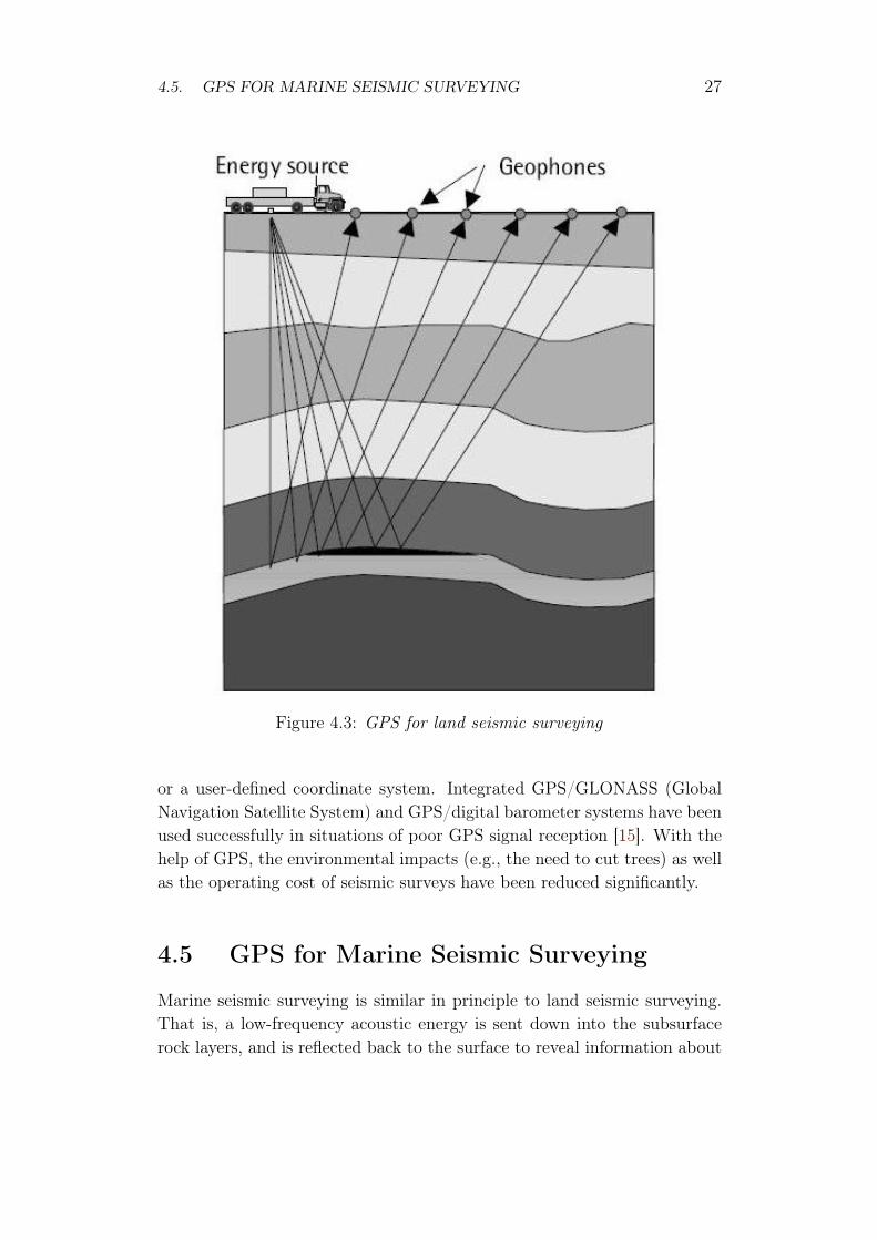
Figure 4.4: GPS for marine seismic surveying
the composition of subsurface rocks (Figure 4.4).
Different methods are used iJ1 marine seismic surveys depending on thewater depth. In deep waters, seismic vessels tow seismic cables, knownas streamers, which contain devices called hydrophones used for detectingreflected energy. A single vessel will normally tow four to eight parallelstreamers; each has a length of several kilometers [14]. The low-frequencyacoustic energy is generated using a number of air guns towed behind thevessel at about 6m below the surface. In shallow waters, both the landand the marine methods are used. Ocean bottom cable (OBC) survey is arelatively new technology that has been used recently for water depth of upto about 200m. In this method, hydrophones and geophones are combinedin a single receiver to avoid water column reverberation (Figure 4.4).
To obtain meaningful results, the positions of the energy source and thehydrophones must be known with sufficient accuracy. This can be eas-ily achieved, at lower cost, with GPS. As the operation of marine seismicsurveys is very expensive, the issue of quality control (QC) is essential. Tomaintain QC, the seismic industry has suggested the use of two independentpositioning systems, with GPS being the primary one [14].
4.6. GPS FOR VEHICLE NAVIGATION 29
Figure 4.5: GPS for vehicle navigation
4.6 GPS for Vehicle Navigation
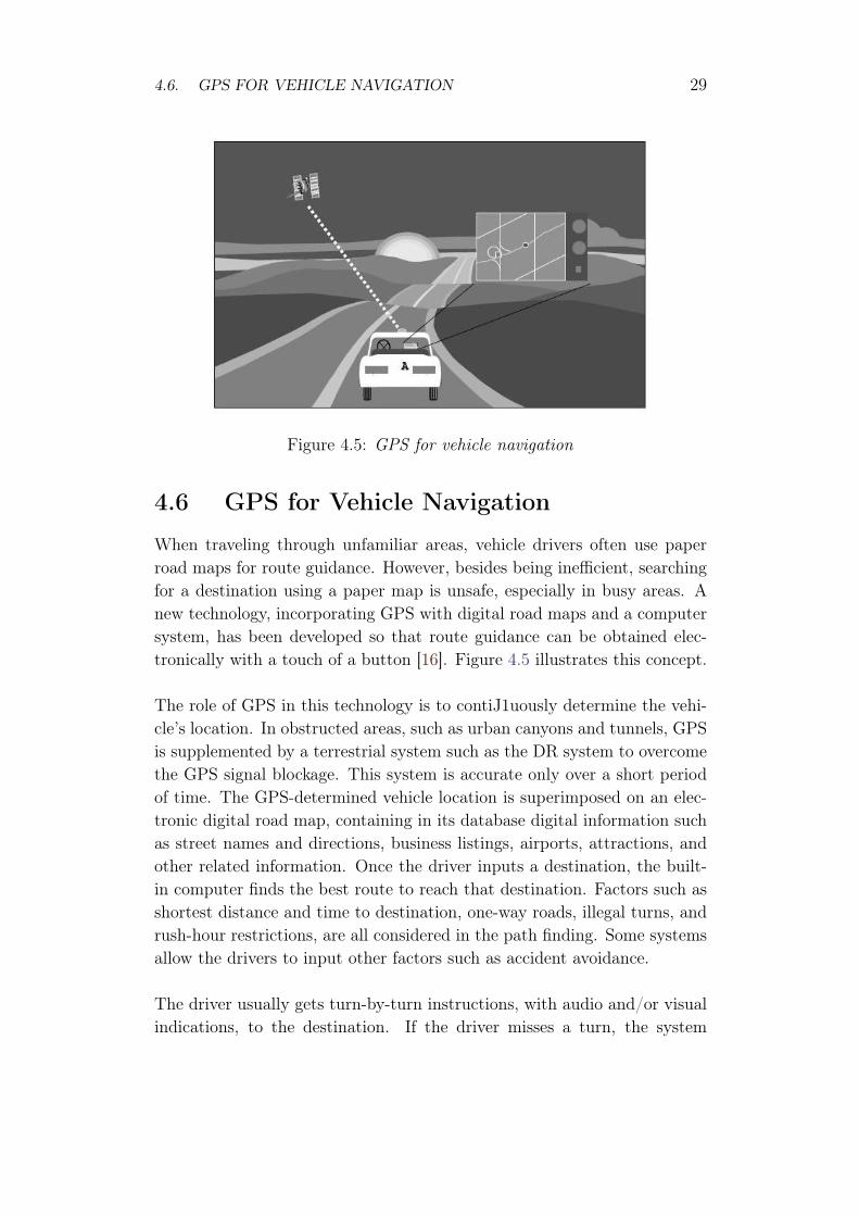
When traveling through unfamiliar areas, vehicle drivers often use paperroad maps for route guidance. However, besides being inefficient, searchingfor a destination using a paper map is unsafe, especially in busy areas. Anew technology, incorporating GPS with digital road maps and a computersystem, has been developed so that route guidance can be obtained elec-tronically with a touch of a button [16]. Figure 4.5 illustrates this concept.
The role of GPS in this technology is to contiJ1uously determine the vehi-cle’s location. In obstructed areas, such as urban canyons and tunnels, GPSis supplemented by a terrestrial system such as the DR system to overcomethe GPS signal blockage. This system is accurate only over a short periodof time. The GPS-determined vehicle location is superimposed on an elec-tronic digital road map, containing in its database digital information suchas street names and directions, business listings, airports, attractions, andother related information. Once the driver inputs a destination, the built-in computer finds the best route to reach that destination. Factors such asshortest distance and time to destination, one-way roads, illegal turns, andrush-hour restrictions, are all considered in the path finding. Some systemsallow the drivers to input other factors such as accident avoidance.
The driver usually gets turn-by-turn instructions, with audio and/or visualindications, to the destination. If the driver misses a turn, the system
30 CHAPTER 4. GLOBAL POSITION SYSTEMS APPLICATIONS
displays a warning message and finds an alternative best route based on thecurrent location of the vehicle. Some manufacturers add cellular systemsto provide weather and traffic information and to locate the vehicles incase of emergency. Recent advances in wireless communication technologyeven make it possible for drivers to remotely access the Internet from theirvehicles [17].
4.7 GPS for Transit Systems
Transit system authorities in many countries are faced with a challengingtrend of fiscal constraints, which limits their capabilities to expand exist-ing services and to increase ridership. Until recently, transit systems usedold technologies such as odometer/compass sensors and signposts for posi-tion determination [18]. odometers are sensors that measure the number ofrotation counts generated by the vehicle’s wheels, which are then used toestimate the distance traveled by the vehicle. With the help of a compass,the vehicle’s direction of travel can be determined at any time. Combiningthe measurements from the odometer and the compass, the vehicle’s posi-tion can be determined with respect to an initial (known) position.
Unfortunately, both the odometer and the compass drift over time, whichcauses significant error in the estimated position. Signposts, in contrast,are radio beacon transmitters that are placed at known locations along thebus routes [19]. Each beacon transmits a low-power microwave signal, whichis detected by a receiver on the bus, to account for the odometer’s drift error.
Unfortunately, this system has a number of limitations, including its inca-pability of knowing the exact location of a vehicle in between two signposts.In addition, it is not possible to track a vehicle that goes off-route as a resultof, for example, a road closure [18].
To overcome the limitations of these systems, transit authorities are inte-grating a low-cost autonomous GPS system with one or more of these con-ventional systems. GPS helps in controlling the drift of the conventionalsystems through frequent calibration. In addition, the vehicle’s position canbe obtained reliably with GPS if the vehicle goes off-route. However, sincesome of the GPS signals will be obstructed in areas with high-rise buildings,such as downtown areas, the vehicle’s position may be obtained with the
4.7. GPS FOR TRANSIT SYSTEMS 31
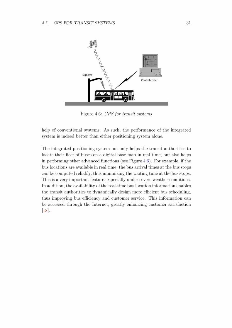
Figure 4.6: GPS for transit systems
help of conventional systems. As such, the performance of the integratedsystem is indeed better than either positioning system alone.
The integrated positioning system not only helps the transit authorities tolocate their fleet of buses on a digital base map in real time, but also helpsin performing other advanced functions (see Figure 4.6). For example, if thebus locations are available in real time, the bus arrival times at the bus stopscan be computed reliably, thus minimizing the waiting time at the bus stops.This is a very important feature, especially under severe weather conditions.In addition, the availability of the real-time bus location information enablesthe transit authorities to dynamically design more efficient bus scheduling,thus improving bus efficiency and customer service. This information canbe accessed through the Internet, greatly enhancing customer satisfaction[18].

Bibliography
[1] Dinesh M., Yongcheol S., Ryosuke S., Technical Repport of IEICE. “GPSSignal Acquisition and Tracking”. The Institute of Electronics, Informationand Communication Engineers. [cited at p. 1]
[2] FRP, U.S. “Federal Radionavigation Plan”, 1999. [cited at p. 1]
[3] Kaplan, E. “Understanding GPS: Principles and Application”, Norwood MA:Artech House 1990. [cited at p. 18]
[4] Langley, R.B, “Why is The GPS signal so Complex?”, GPS World, Vol. 1,No. 3 May/June 1990, pp. 56–59. [cited at p. 1]
[5] Langley, R.B, “The mathematic of GPS”, GPS World, Vol. 2, No. 7July/August 1991, pp. 45–50. [cited at p. 17]
[6] Peyton Z., Peebles, JR. Tata eds. 2001. “Probability, Random Variables andRandom Signal principles”. Tata McGraw-Hill Publishing Company Limited.New Delhi. [cited at p. 8, 9, 11]
[7] Nail H. Ibragimov. eds. 2006. “A Practical Course in Differential Equa-tions and Mathematical Modelling”. ALGA Publication, Blekinge Instituteof Technology. [cited at p. 8, 10]
[8] Institute of Navigation. “Global Positioning System monographs”. Washing-ton, DC: The Institute of Navigation. [cited at p. 2]
[9] Global Positioning System “Standard Positioning Service Specification”, 2ndEdition, June2, 1995. [cited at p. 16]
[10] Laser Technology Inc., “Survey Laser for Forestery”,Powerpoint Presentation,access July 18, 2001, www.lasertech.com/download.html. [cited at p. 24]
[11] Smith, B. S., “GPS Grade Control for Construction”, Smith, B. S., "GPSGrade Control for Construction," Proc. ION GPS 2000, 13th Intl. Techni-
33
34 BIBLIOGRAPHY
cal Meeting, Satellite Division, Institute of Navigation, Salt Lake City, UT,September 19-22, 2000, pp. 1034–1037. [cited at p. 25]
[12] Elfick, M., et al., “Elementary Surveying”, 8th Edition, Newy York: Harper-Collins, 1994. [cited at p. 25]
[13] El-Rabbany, A.,A. Chrzanowski, and M. Santos, “GPS Application in CivilEngineering ”, Ontario Land Surveyor Quaterly 2001, pp. 6–8. [cited at p. 25]
[14] Jensen, M.H “Quality Control for Differential GPS on Offshore Oil andGaz Exploration”, GPS World, Vol. 3, No. 8 September 1992, pp. 36–48.[cited at p. 26, 28]
[15] McLintock, D.,G. Deren and E. Krakwisky “Environment Sensitive: DGPSand Barometry for Seismic Survey ”, GPS World, Vol. 3, No. 8 February1994, pp. 20-26. [cited at p. 27]
[16] Zhao, Y., “Vehicle Location and Navigation Systems”, Nonvood, MA: ArtechHouse, 1997. [cited at p. 29]
[17] Hada, H., et al., “The Internet, Cars, and DGPS: Bringing Mobile Sensorsand Global Correction Services On Line,” GPS World, Vol. 11, No.5, May2000, pp. 38–43. [cited at p. 30]
[18] El-Rabbany, A., A. Shabby, and S. Zolfaghari, “Real-Time Bus Location,Passenger Information and Scheduling for Public Transportation,” Presentedat GPS meeting, GOEIDE 2000 Conference, Calgary, Alberta, Canada, May24–26, 2000. [cited at p. 30, 31]
[19] Drane, C., and C. Rizos, “Positionillg Systems in Intelligent TransportationSystems”, Norwood, MA: Artech House, 1998. [cited at p. 30]

Appendices
35

Appendix A
GPS Source Code for Data Acquisition
37
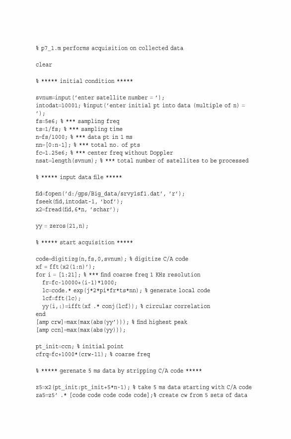
% p7 1.m performs acquisition on collected data
clear
% ***** initial condition *****
svnumcinput(’enter satellite number c ’);intodatc10001; %input(’enter initial pt into data (multiple of n) c’);fsc5e6; % *** sampling freqtsc1/fs; % *** sampling timencfs/1000; % *** data pt in 1 msnnc[0:n-1]; % *** total no. of ptsfcc1.25e6; % *** center freq without Dopplernsatclength(svnum); % *** total number of satellites to be processed
% ***** input data file *****
fidcfopen(’d:/gps/Big data/srvy1sf1.dat’, ’r’);fseek(fid,intodat-1, ’bof’);x2cfread(fid,6*n, ’schar’);
yy c zeros(21,n);
% ***** start acquisition *****
codecdigitizg(n,fs,0,svnum); % digitize C/A codexf c fft(x2(1:n)’);for i c [1:21]; % *** find coarse freq 1 KHz resolutionfrcfc-10000+(i-1)*1000;lcccode.* exp(j*2*pi*fr*ts*nn); % generate local codelcfcfft(lc);yy(i,:)cifft(xf .* conj(lcf)); % circular correlation
end[amp crw]cmax(max(abs(yy’))); % find highest peak[amp ccn]cmax(max(abs(yy)));
pt initcccn; % initial pointcfrqcfc+1000*(crw-11); % coarse freq
% ***** gerenate 5 ms data by stripping C/A code *****
z5cx2(pt init:pt init+5*n-1); % take 5 ms data starting with C/A codeza5cz5’ .* [code code code code code];% create cw from 5 sets of data
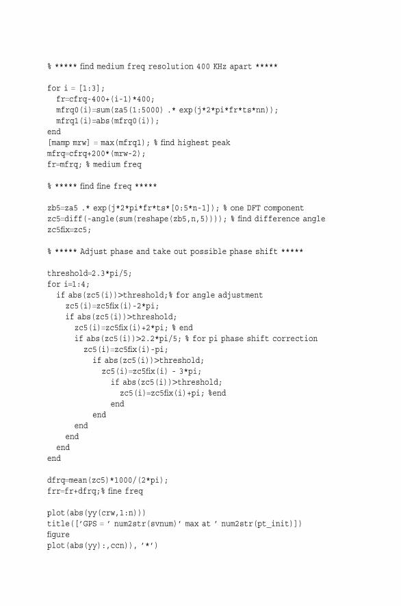
% ***** find medium freq resolution 400 KHz apart *****
for i c [1:3];frccfrq-400+(i-1)*400;mfrq0(i)csum(za5(1:5000) .* exp(j*2*pi*fr*ts*nn));mfrq1(i)cabs(mfrq0(i));
end[mamp mrw] c max(mfrq1); % find highest peakmfrqccfrq+200*(mrw-2);frcmfrq; % medium freq
% ***** find fine freq *****
zb5cza5 .* exp(j*2*pi*fr*ts*[0:5*n-1]); % one DFT componentzc5cdiff(-angle(sum(reshape(zb5,n,5)))); % find difference anglezc5fixczc5;
% ***** Adjust phase and take out possible phase shift *****
thresholdc2.3*pi/5;for ic1:4;if abs(zc5(i))>threshold;% for angle adjustmentzc5(i)czc5fix(i)-2*pi;if abs(zc5(i))>threshold;zc5(i)czc5fix(i)+2*pi; % endif abs(zc5(i))>2.2*pi/5; % for pi phase shift correctionzc5(i)czc5fix(i)-pi;
if abs(zc5(i))>threshold;zc5(i)czc5fix(i) - 3*pi;
if abs(zc5(i))>threshold;zc5(i)czc5fix(i)+pi; %end
endend
endend
endend
dfrqcmean(zc5)*1000/(2*pi);frrcfr+dfrq;% fine freq
plot(abs(yy(crw,1:n)))title([’GPS c ’ num2str(svnum)’ max at ’ num2str(pt init)])figureplot(abs(yy):,ccn)), ’*’)
% title([’GPS c ’ num2str(svnum) ’ Freq c ’ num2str(frr)])formatpt initformat long efrr
% digitizg.m This prog generates the C/A code and digitizes itfunction code2 c digitizg(n,fs,offset,svnum);
% code - gold code% n - number of samples% fs - sample frequency in Hz;% offset - delay time in seconds must be less than 1/fs cannot shiftleft% svnum - satellite number;
gold rate c 1.023e6; %gold code clock rate in Hz.tsc1/fs;tcc1/gold rate;
cmd1 c codegen(svnum); % generate C/A codecode inccdm1;
% ***** creating 16 C/A code for digitizing *****
code a c [code in code in code in code in];code ac[code a code a];code ac[code a code a];
% ***** digitizing *****
b c [1:n];c c ceil((ts*b+offset)/tc);code c code a(c);
% ***** adjusting first data point *****
if offset>c0;code2c[code(1) code(1:n-1)];
elsecode2c[code(n) code(1:n-1)];
end

function [ca used]ccodegen(svnum);
% ca used : a vector containing the desired output sequence% the g2s vector holds the appropriate shift of the g2 code to generate% the C/A code (ex. for SV#19 - use a G2 shift of g2s(19)c471)% svnum: Satellite number
gs2 c [5;6;7;8;17;18;139;140;141;251;252;254;255;256;257;258;469;470;471; ... 472;473;474;509;512;513;514;515;516;859;860;861;862];
g2shiftcg2s(svnum,1);
% ***** Generate G1 code *****
% load shift registerreg c -1*ones(1,10);
for i c 1:1023,g1(i) c reg(10);save1 c reg(3)*reg(10);reg(1,2:10) c reg(1:1:9);reg(1) c save1;
end,
% ***** Generate G2 code *****% load shift register
reg c -1*ones(1,10);for i c 1:1023,
g2(i) c reg(10);save2 c reg(2)*reg(3)*reg(6)*reg(8)*reg(9)*reg(10);reg(1,2:10) c reg(1:1:9);reg(1) c save2;
end
% ***** Shift G2 code *****g2tmp(1,1:g2shift)cg2(1,1023-g2shift+1:1023);g2tmp(1,g2shift+1:1023)cg2(1,1:1023-g2shift);g2 c g2tmp;
% ***** Form single sample C/A code by multiplying G1 and G2
ss ca c g1.*g2;ca usedc-ss ca;