Embed Size (px)
Citation preview
The Finite Element Method for the Analysis ofNon-Linear and Dynamic Systems
Prof. Dr. Eleni Chatzi
Lecture 1 - 17 September, 2015
Institute of Structural Engineering Method of Finite Elements II 1
Course Information
InstructorProf. Dr. Eleni Chatzi, email: [email protected] Hours: HIL E14.3, Wednesday 10:00-12:00 or by email
AssistantAdrian Egger, HIL E13.1, email: [email protected]
Course WebsiteLecture Notes and Homeworks will be posted at:http://www.chatzi.ibk.ethz.ch/education/method-of-finite-elements-ii.html
Suggested Reading
“Nonlinear Finite Elements for Continua and Structures”, by T.Belytschko, W. K. Liu, and B. Moran, John Wiley and Sons, 2000
“The Finite Element Method: Linear Static and Dynamic FiniteElement Analysis”, by T. J. R. Hughes, Dover Publications, 2000
Lecture Notes by Carlos A. FelippaNonlinear Finite Element Methods (ASEN 6107): http://www.
colorado.edu/engineering/CAS/courses.d/NFEM.d/Home.html
Institute of Structural Engineering Method of Finite Elements II 2
Course Outline
Review of the Finite Element method - Introduction toNon-Linear Analysis
Non-Linear Finite Elements in solids and Structural Mechanics- Overview of Solution Methods- Continuum Mechanics & Finite Deformations- Lagrangian Formulation
- Structural Elements
Dynamic Finite Element Calculations- Integration Methods
- Mode Superposition
Eigenvalue Problems
Special Topics- The Scaled Boundary Element & Extended Finite Element methods
Institute of Structural Engineering Method of Finite Elements II 3

Grading Policy
Performance Evaluation - Homeworks (100%)
Homework
Homeworks are due in class within 3 weeks after assignment
Computer Assignments may be done using any coding language(MATLAB, Fortran, C, MAPLE) - example code will beprovided in MATLAB
Commercial software such as ABAQUS and SAP will also beused for certain Assignments
Homework Sessions will be pre-announced and it is advised to bringa laptop along for those sessions
Help us Structure the Course!Participate in our online survey:http://goo.gl/forms/ws0ASBLXiY
Institute of Structural Engineering Method of Finite Elements II 4
Lecture #1: Structure
Let us review the Linear Finite Element Method
Strong vs. Weak Formulation
The Finite Element (FE) formulation
The Iso-Parametric Mapping
Structural Finite Elements
The Bar Element
The Beam Element
Example
The Axially Loaded Bar
Institute of Structural Engineering Method of Finite Elements II 5
Review of the Finite Element Method (FEM)
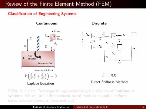
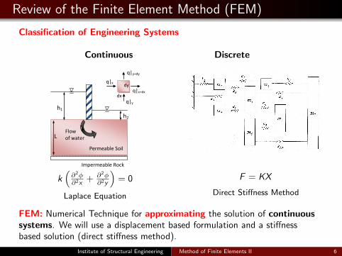
Classification of Engineering Systems
Continuous Discrete
h2
h1
Permeable Soil
Flow of water
L
Impermeable Rock
dx
dy
q|y
q|x+dx
q|y+dy
q|x
k(∂2φ∂2x + ∂2φ
∂2y
)= 0
Laplace Equation
F = KX
Direct Stiffness Method
FEM: Numerical Technique for approximating the solution of continuoussystems. We will use a displacement based formulation and a stiffnessbased solution (direct stiffness method).
Institute of Structural Engineering Method of Finite Elements II 6
Review of the Finite Element Method (FEM)
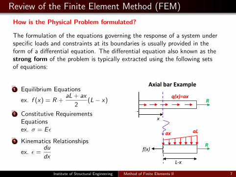
How is the Physical Problem formulated?
The formulation of the equations governing the response of a system underspecific loads and constraints at its boundaries is usually provided in theform of a differential equation. The differential equation also known as thestrong form of the problem is typically extracted using the following setsof equations:
1 Equilibrium Equations
ex. f (x) = R +aL + ax
2(L− x)
2 Constitutive RequirementsEquationsex. σ = Eε
3 Kinematics Relationships
ex. ε =du
dx
x
R q(x)=ax
aL
R
ax
L-x
Axial bar Example
f(x)
Institute of Structural Engineering Method of Finite Elements II 7
Review of the Finite Element Method (FEM)
How is the Physical Problem formulated?
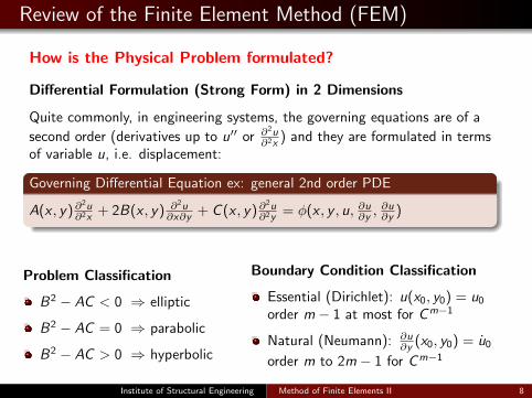
Differential Formulation (Strong Form) in 2 Dimensions
Quite commonly, in engineering systems, the governing equations are of a
second order (derivatives up to u′′ or ∂2u∂2x ) and they are formulated in terms
of variable u, i.e. displacement:
Governing Differential Equation ex: general 2nd order PDE
A(x , y)∂2u∂2x + 2B(x , y) ∂2u
∂x∂y + C (x , y)∂2u∂2y = φ(x , y , u, ∂u∂y ,
∂u∂y )
Problem Classification
B2 − AC < 0 ⇒ elliptic
B2 − AC = 0 ⇒ parabolic
B2 − AC > 0 ⇒ hyperbolic
Boundary Condition Classification
Essential (Dirichlet): u(x0, y0) = u0
order m − 1 at most for Cm−1
Natural (Neumann): ∂u∂y (x0, y0) = u0
order m to 2m − 1 for Cm−1
Institute of Structural Engineering Method of Finite Elements II 8
Review of the Finite Element Method (FEM)
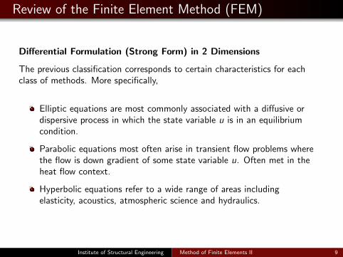
Differential Formulation (Strong Form) in 2 Dimensions
The previous classification corresponds to certain characteristics for eachclass of methods. More specifically,
Elliptic equations are most commonly associated with a diffusive ordispersive process in which the state variable u is in an equilibriumcondition.
Parabolic equations most often arise in transient flow problems wherethe flow is down gradient of some state variable u. Often met in theheat flow context.
Hyperbolic equations refer to a wide range of areas includingelasticity, acoustics, atmospheric science and hydraulics.
Institute of Structural Engineering Method of Finite Elements II 9
Strong Form - 1D FEM
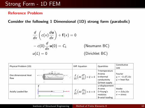
Reference Problem
Consider the following 1 Dimensional (1D) strong form (parabolic)
d
dx
(c(x)
du
dx
)+ f(x) = 0
− c(0)d
dxu(0) = C1 (Neumann BC)
u(L) = 0 (Dirichlet BC)
Physical Problem (1D) Diff. Equation Quantities Constitutive Law
One dimensional Heat flow
𝑑𝑑𝑥
𝐴𝑘𝑑𝑇𝑑𝑥
+ 𝑄 = 0
T=temperature A=area k=thermal conductivity Q=heat supply
Fourier 𝑞 = −𝑘 𝑑𝑇/𝑑𝑥 𝑞 = heat flux
Axially Loaded Bar
𝑑𝑑𝑥
𝐴𝐸𝑑𝑢𝑑𝑥
+ 𝑏 = 0
u=displacement A=area E=Young’s modulus B=axial loading
Hooke 𝜎 = 𝐸𝑑𝑢/𝑑𝑥 𝜎 = stress
Institute of Structural Engineering Method of Finite Elements II 10
Weak Form - 1D FEM
Approximating the Strong Form
The strong form requires strong continuity on the dependent fieldvariables (usually displacements). Whatever functions define thesevariables have to be differentiable up to the order of the PDE thatexist in the strong form of the system equations. Obtaining theexact solution for a strong form of the system equation is a quitedifficult task for practical engineering problems.
The finite difference method can be used to solve the systemequations of the strong form and obtain an approximate solution.However, this method usually works well for problems with simpleand regular geometry and boundary conditions.
Alternatively we can use the finite element method on a weakform of the system. This weak form is usually obtained throughenergy principles which is why it is also known as variational form.
Institute of Structural Engineering Method of Finite Elements II 11
Weak Form - 1D FEM
From Strong Form to Weak form
Three are the approaches commonly used to go from strong to weakform:
Principle of Virtual Work
Principle of Minimum Potential Energy
Methods of weighted residuals (Galerkin, Collocation, LeastSquares methods, etc)
Visit our Course page on Linear FEM for further details:http://www.chatzi.ibk.ethz.ch/education/
method-of-finite-elements-i.html
Institute of Structural Engineering Method of Finite Elements II 12
Weak Form - 1D FEM
From Strong Form to Weak form - Approach #1
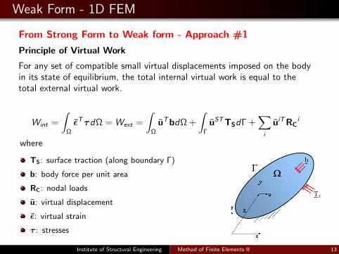
Principle of Virtual Work
For any set of compatible small virtual displacements imposed on the bodyin its state of equilibrium, the total internal virtual work is equal to thetotal external virtual work.
Wint =
∫Ω
εTτdΩ = Wext =
∫Ω
uTbdΩ +
∫Γ
uSTTSdΓ +∑i
uiTRCi
where
TS: surface traction (along boundary Γ)
b: body force per unit area
RC: nodal loads
u: virtual displacement
ε: virtual strain
τ : stresses
Institute of Structural Engineering Method of Finite Elements II 13
Weak Form - 1D FEM
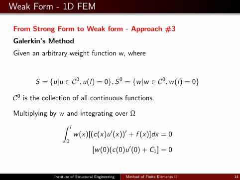
From Strong Form to Weak form - Approach #3
Galerkin’s Method
Given an arbitrary weight function w, where
S = u|u ∈ C0, u(l) = 0,S0 = w |w ∈ C0,w(l) = 0
C0 is the collection of all continuous functions.
Multiplying by w and integrating over Ω∫ l
0w(x)[(c(x)u′(x))′ + f (x)]dx = 0
[w(0)(c(0)u′(0) + C1] = 0
Institute of Structural Engineering Method of Finite Elements II 14
Weak Form - 1D FEM
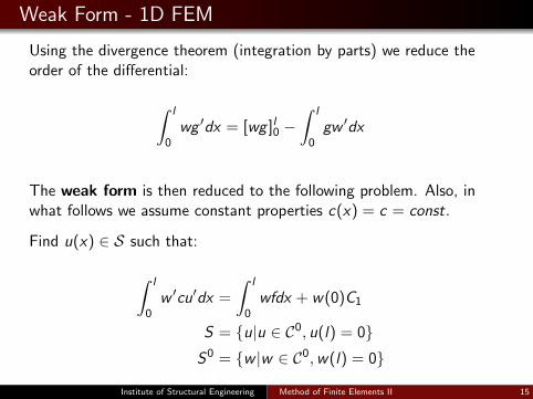
Using the divergence theorem (integration by parts) we reduce theorder of the differential:
∫ l
0wg ′dx = [wg ]l0 −
∫ l
0gw ′dx
The weak form is then reduced to the following problem. Also, inwhat follows we assume constant properties c(x) = c = const.
Find u(x) ∈ S such that:
∫ l
0w ′cu′dx =
∫ l
0wfdx + w(0)C1
S = u|u ∈ C0, u(l) = 0S0 = w |w ∈ C0,w(l) = 0
Institute of Structural Engineering Method of Finite Elements II 15
Weak Form
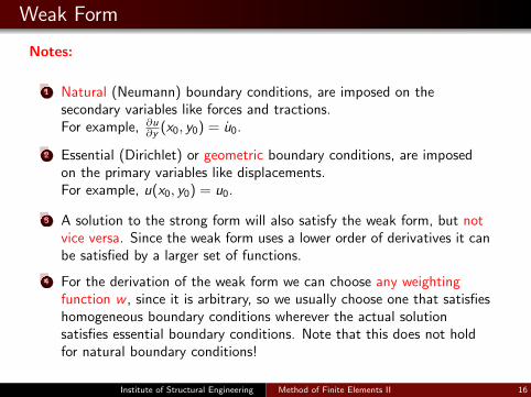
Notes:
1 Natural (Neumann) boundary conditions, are imposed on thesecondary variables like forces and tractions.For example, ∂u
∂y (x0, y0) = u0.
2 Essential (Dirichlet) or geometric boundary conditions, are imposedon the primary variables like displacements.For example, u(x0, y0) = u0.
3 A solution to the strong form will also satisfy the weak form, but notvice versa. Since the weak form uses a lower order of derivatives it canbe satisfied by a larger set of functions.
4 For the derivation of the weak form we can choose any weightingfunction w , since it is arbitrary, so we usually choose one that satisfieshomogeneous boundary conditions wherever the actual solutionsatisfies essential boundary conditions. Note that this does not holdfor natural boundary conditions!
Institute of Structural Engineering Method of Finite Elements II 16
FE formulation: Discretization
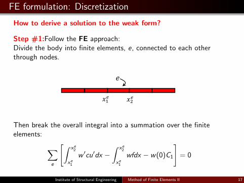
How to derive a solution to the weak form?
Step #1:Follow the FE approach:Divide the body into finite elements, e, connected to each otherthrough nodes.
𝑥1𝑒 𝑥2𝑒
𝑒
Then break the overall integral into a summation over the finiteelements:
∑e
[∫ xe2
xe1
w ′cu′dx −∫ xe2
xe1
wfdx − w(0)C1
]= 0
Institute of Structural Engineering Method of Finite Elements II 17
1D FE formulation: Galerkin’s Method
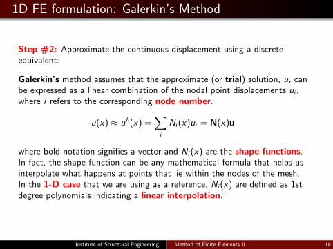
Step #2: Approximate the continuous displacement using a discreteequivalent:
Galerkin’s method assumes that the approximate (or trial) solution, u, canbe expressed as a linear combination of the nodal point displacements ui ,where i refers to the corresponding node number.
u(x) ≈ uh(x) =∑i
Ni (x)ui = N(x)u
where bold notation signifies a vector and Ni (x) are the shape functions.In fact, the shape function can be any mathematical formula that helps usinterpolate what happens at points that lie within the nodes of the mesh.In the 1-D case that we are using as a reference, Ni (x) are defined as 1stdegree polynomials indicating a linear interpolation.
Institute of Structural Engineering Method of Finite Elements II 18
1D FE formulation: Galerkin’s Method
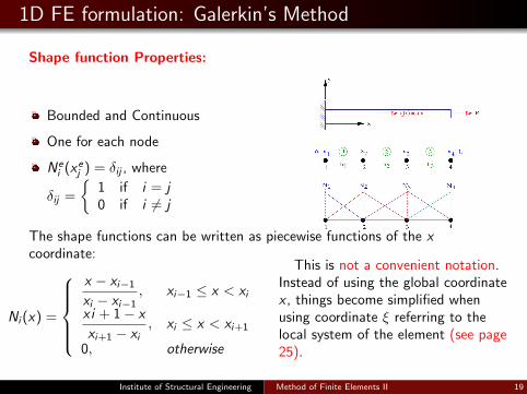
Shape function Properties:
Bounded and Continuous
One for each node
Nei (xej ) = δij , where
δij =
1 if i = j0 if i 6= j
The shape functions can be written as piecewise functions of the xcoordinate:
Ni (x) =
x − xi−1
xi − xi−1, xi−1 ≤ x < xi
xi + 1− x
xi+1 − xi, xi ≤ x < xi+1
0, otherwise
This is not a convenient notation.Instead of using the global coordinatex , things become simplified whenusing coordinate ξ referring to thelocal system of the element (see page25).
Institute of Structural Engineering Method of Finite Elements II 19
1D FE formulation: Galerkin’s Method
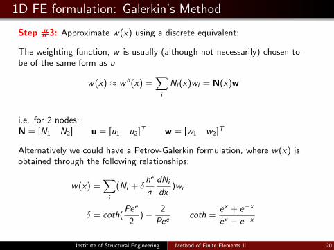
Step #3: Approximate w(x) using a discrete equivalent:
The weighting function, w is usually (although not necessarily) chosen tobe of the same form as u
w(x) ≈ wh(x) =∑i
Ni (x)wi = N(x)w
i.e. for 2 nodes:N = [N1 N2] u = [u1 u2]T w = [w1 w2]T
Alternatively we could have a Petrov-Galerkin formulation, where w(x) isobtained through the following relationships:
w(x) =∑i
(Ni + δhe
σ
dNi
dx)wi
δ = coth(Pee
2)− 2
Peecoth =
ex + e−x
ex − e−x
Institute of Structural Engineering Method of Finite Elements II 20
1D FE formulation: Galerkin’s Method
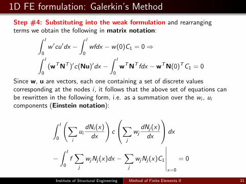
Step #4: Substituting into the weak formulation and rearrangingterms we obtain the following in matrix notation:∫ l
0
w ′cu′dx −∫ l
0
wfdx − w(0)C1 = 0⇒∫ l
0
(wTNT )′c(Nu)′dx −∫ l
0
wTNT fdx −wTN(0)TC1 = 0
Since w, u are vectors, each one containing a set of discrete valuescorresponding at the nodes i , it follows that the above set of equations canbe rewritten in the following form, i.e. as a summation over the wi , uicomponents (Einstein notation):
∫ l
0
(∑i
uidNi (x)
dx
)c
∑j
wjdNj(x)
dx
dx
−∫ l
0
f∑j
wjNj(x)dx −∑j
wjNj(x)C1
∣∣∣∣∣∣x=0
= 0
Institute of Structural Engineering Method of Finite Elements II 21
1D FE formulation: Galerkin’s Method
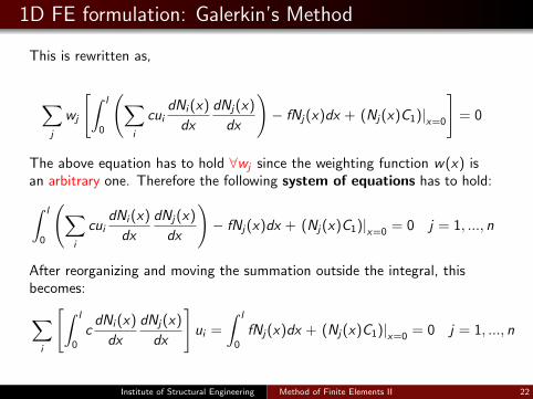
This is rewritten as,
∑j
wj
[∫ l
0
(∑i
cuidNi (x)
dx
dNj(x)
dx
)− fNj(x)dx + (Nj(x)C1)|x=0
]= 0
The above equation has to hold ∀wj since the weighting function w(x) isan arbitrary one. Therefore the following system of equations has to hold:∫ l
0
(∑i
cuidNi (x)
dx
dNj(x)
dx
)− fNj(x)dx + (Nj(x)C1)|x=0 = 0 j = 1, ..., n
After reorganizing and moving the summation outside the integral, thisbecomes:
∑i
[∫ l
0
cdNi (x)
dx
dNj(x)
dx
]ui =
∫ l
0
fNj(x)dx + (Nj(x)C1)|x=0 = 0 j = 1, ..., n
Institute of Structural Engineering Method of Finite Elements II 22
1D FE formulation: Galerkin’s Method
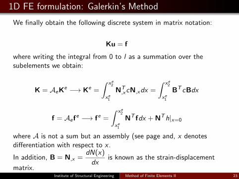
We finally obtain the following discrete system in matrix notation:
Ku = f
where writing the integral from 0 to l as a summation over thesubelements we obtain:
K = AeKe −→ Ke =
∫ xe2
xe1
NT,xcN,xdx =
∫ xe2
xe1
BT cBdx
f = Aefe −→ fe =
∫ xe2
xe1
NT fdx + NTh|x=0
where A is not a sum but an assembly (see page and, x denotesdifferentiation with respect to x .
In addition, B = N,x =dN(x)
dxis known as the strain-displacement
matrix.Institute of Structural Engineering Method of Finite Elements II 23
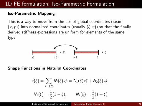
1D FE formulation: Iso-Parametric Formulation
Iso-Parametric Mapping
This is a way to move from the use of global coordinates (i.e.in(x , y)) into normalized coordinates (usually (ξ, η)) so that the finallyderived stiffness expressions are uniform for elements of the sametype.
𝑥1𝑒 𝑥2𝑒 −1 1
𝑥 𝜉
Shape Functions in Natural Coordinates
x(ξ) =∑i=1,2
Ni (ξ)xei = N1(ξ)xe1 + N2(ξ)xe2
N1(ξ) =1
2(1− ξ), N2(ξ) =
1
2(1 + ξ)
Institute of Structural Engineering Method of Finite Elements II 24
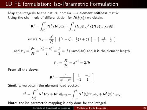
1D FE formulation: Iso-Parametric Formulation
Map the integrals to the natural domain −→ element stiffness matrix.Using the chain rule of differentiation for N(ξ(x)) we obtain:
Ke =
∫ xe2
xe1
NT,xcN,xdx =
∫ 1
−1
(N,ξξ,x)T c(N,ξξ,x)x,ξdξ
where N,ξ =d
dξ
[12(1− ξ) 1
2(1 + ξ)
]=[ −1
212
]and x,ξ =
dx
dξ=
xe2 − xe
1
2=
h
2= J (Jacobian) and h is the element length
ξ,x =dξ
dx= J−1 = 2/h
From all the above,
Ke =c
xe2 − xe
1
[1 −1−1 1
]Similary, we obtain the element load vector:
fe =
∫ xe2
xe1
NT fdx + NTh|x=0 =
∫ 1
−1
NT (ξ)fx,ξdξ + NT(x)h|x=0
Note: the iso-parametric mapping is only done for the integral.
Institute of Structural Engineering Method of Finite Elements II 25
The Beam Element
Discussion & LimitationsWhat are some of the main Assumptions & Simplifications wehave performed so far in the Linear Theory?
What do you imagine are the added problems beyond thisrealm?
Institute of Structural Engineering Method of Finite Elements II 26
The Beam Element
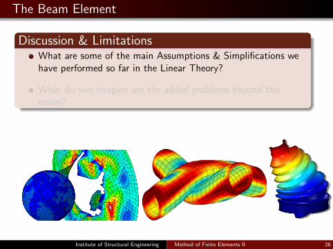
Discussion & LimitationsWhat are some of the main Assumptions & Simplifications wehave performed so far in the Linear Theory?
What do you imagine are the added problems beyond thisrealm?
Institute of Structural Engineering Method of Finite Elements II 26
The Beam Element
Discussion & LimitationsWhat are some of the main Assumptions & Simplifications wehave performed so far in the Linear Theory?
What do you imagine are the added problems beyond thisrealm?
Institute of Structural Engineering Method of Finite Elements II 26
The Beam Element
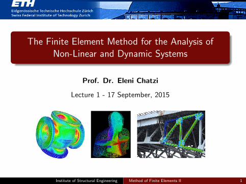
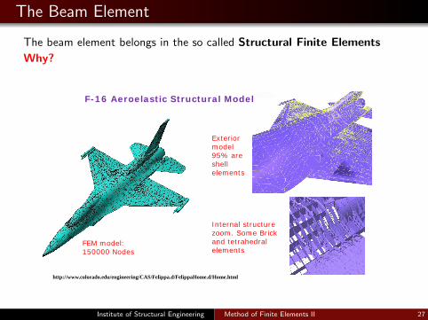
The beam element belongs in the so called Structural Finite Elements
Why?
http://www.colorado.edu/engineering/CAS/Felippa.d/FelippaHome.d/Home.html
FEM model:150000 Nodes
F-16 Aeroelastic Structural Model
Exterior model95% are shell elements
Internal structure zoom. Some Brick and tetrahedralelements
Institute of Structural Engineering Method of Finite Elements II 27
Beam Elements
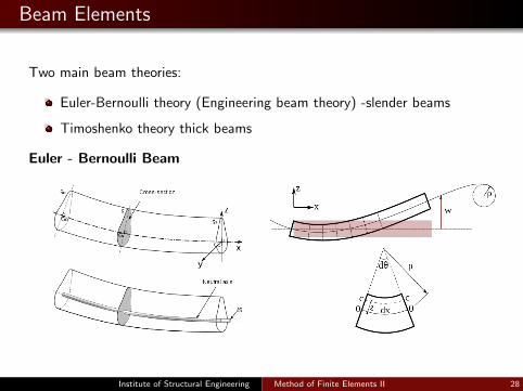
Two main beam theories:
Euler-Bernoulli theory (Engineering beam theory) -slender beams
Timoshenko theory thick beams
Euler - Bernoulli Beam
Institute of Structural Engineering Method of Finite Elements II 28
Beam Elements
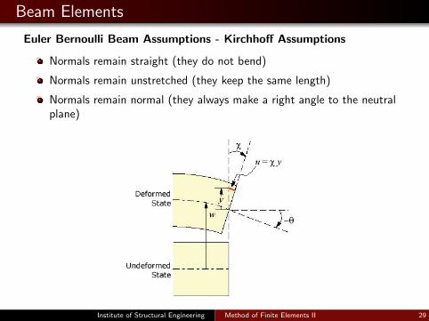
Euler Bernoulli Beam Assumptions - Kirchhoff Assumptions
Normals remain straight (they do not bend)
Normals remain unstretched (they keep the same length)
Normals remain normal (they always make a right angle to the neutralplane)
Institute of Structural Engineering Method of Finite Elements II 29
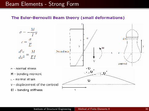
Beam Elements - Strong Form
υ υ
υ
Institute of Structural Engineering Method of Finite Elements II 30
Beam Elements - Strong Form
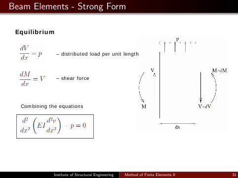
Equilibrium
– distributed load per unit length
– shear force
Combining the equations
Institute of Structural Engineering Method of Finite Elements II 31
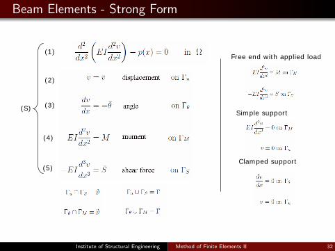
Beam Elements - Strong Form
(S)
Free end with applied load
Simple support
Clamped support
(1)
(2)
(4)
(5)
(3)
Institute of Structural Engineering Method of Finite Elements II 32
Cheat Sheet
Basic Formulas-Shape Functions
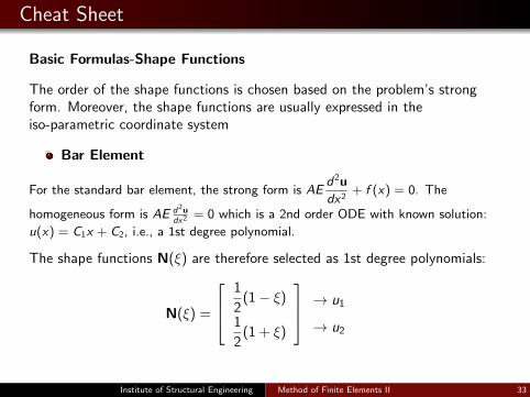
The order of the shape functions is chosen based on the problem’s strongform. Moreover, the shape functions are usually expressed in theiso-parametric coordinate system
Bar Element
For the standard bar element, the strong form is AEd2u
dx2+ f (x) = 0. The
homogeneous form is AE d2udx2 = 0 which is a 2nd order ODE with known solution:
u(x) = C1x + C2, i.e., a 1st degree polynomial.
The shape functions N(ξ) are therefore selected as 1st degree polynomials:
N(ξ) =
1
2(1− ξ)
1
2(1 + ξ)
→ u1
→ u2
Institute of Structural Engineering Method of Finite Elements II 33
Cheat Sheet
Basic Formulas-Shape Functions
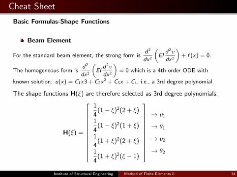
Beam Element
For the standard beam element, the strong form isd2
dx2
(EI
d2υ
dx2
)+ f (x) = 0.
The homogeneous form isd2
dx2
(EI
d2υ
dx2
)= 0 which is a 4th order ODE with
known solution: u(x) = C1x3 + C2x2 + C3x + C4, i.e., a 3rd degree polynomial.
The shape functions H(ξ) are therefore selected as 3rd degree polynomials:
H(ξ) =
1
4(1− ξ)2(2 + ξ)
1
4(1− ξ)2(1 + ξ)
1
4(1 + ξ)2(2 + ξ)
1
4(1 + ξ)2(ξ − 1)
→ u1
→ θ1
→ u2
→ θ2
Institute of Structural Engineering Method of Finite Elements II 34
Cheat Sheet
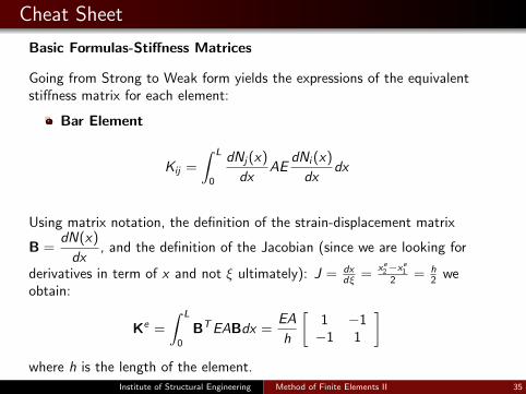
Basic Formulas-Stiffness Matrices
Going from Strong to Weak form yields the expressions of the equivalentstiffness matrix for each element:
Bar Element
Kij =
∫ L
0
dNj(x)
dxAE
dNi (x)
dxdx
Using matrix notation, the definition of the strain-displacement matrix
B =dN(x)
dx, and the definition of the Jacobian (since we are looking for
derivatives in term of x and not ξ ultimately): J = dxdξ =
xe2−x
e1
2 = h2 we
obtain:
Ke =
∫ L
0
BTEABdx =EA
h
[1 −1−1 1
]where h is the length of the element.
Institute of Structural Engineering Method of Finite Elements II 35
Cheat Sheet
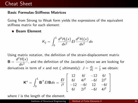
Basic Formulas-Stiffness Matrices
Going from Strong to Weak form yields the expressions of the equivalentstiffness matrix for each element:
Beam Element
Kij =
∫ L
0
d2Hj(x)
dx2EI
d2Hi (x)
dx2dx
Using matrix notation, the definition of the strain-displacement matrix
B =d2H(x)
dx2, and the definition of the Jacobian (since we are looking for
derivatives in term of x and not ξ ultimately): J = dxdξ = l
2 we obtain:
Ke =
∫ L
0
BTEIBdx =EI
l3
12 6l −12 6l6l 4l2 −6l 2l2
−12 −6l 12 −6l6l 2l2 −6l 4l2
where l is the length of the element.
Institute of Structural Engineering Method of Finite Elements II 36
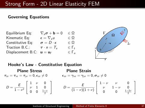
Strong Form - 2D Linear Elasticity FEM
Governing Equations
Equilibrium Eq: ∇sσ + b = 0 ∈ ΩKinematic Eq: ε = ∇su ∈ ΩConstitutive Eq: σ = D · ε ∈ ΩTraction B.C.: τ · n = Ts ∈ Γt
Displacement B.C: u = uΓ ∈ Γu
Hooke’s Law - Constitutive Equation
Plane Stressτzz = τxz = τyz = 0, εzz 6= 0
D =E
1− ν2
1 ν 0ν 1 00 0 1−ν
2
Plane Strain
εzz = γxz = γyz = 0,σzz 6= 0
D =E
(1− ν)(1 + ν)
1− ν ν 0ν 1− ν 00 0 1−2ν
2
Institute of Structural Engineering Method of Finite Elements II 37
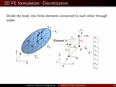
2D FE formulation: Discretization
Divide the body into finite elements connected to each other throughnodes
Institute of Structural Engineering Method of Finite Elements II 38
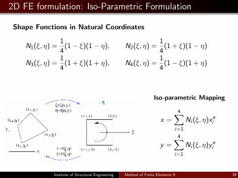
2D FE formulation: Iso-Parametric Formulation
Shape Functions in Natural Coordinates
N1(ξ, η) =1
4(1− ξ)(1− η), N2(ξ, η) =
1
4(1 + ξ)(1− η)
N3(ξ, η) =1
4(1 + ξ)(1 + η), N4(ξ, η) =
1
4(1− ξ)(1 + η)
Iso-parametric Mapping
x =4∑
i=1
Ni (ξ, η)xei
y =4∑
i=1
Ni (ξ, η)y ei
Institute of Structural Engineering Method of Finite Elements II 39
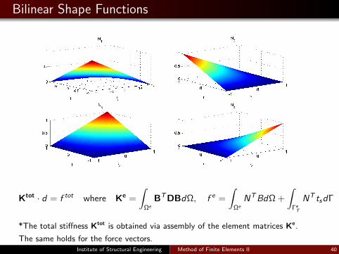
Bilinear Shape Functions
Ktot · d = f tot where Ke =
∫Ωe
BTDBdΩ, f e =
∫Ωe
NTBdΩ +
∫ΓeT
NT tsdΓ
*The total stiffness Ktot is obtained via assembly of the element matrices Ke.
The same holds for the force vectors.Institute of Structural Engineering Method of Finite Elements II 40
Axially Loaded Bar Example
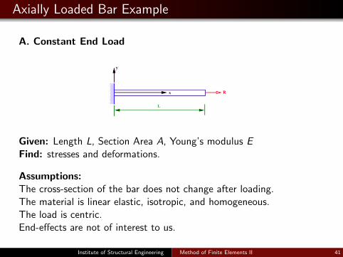
A. Constant End Load
Given: Length L, Section Area A, Young’s modulus EFind: stresses and deformations.
Assumptions:The cross-section of the bar does not change after loading.The material is linear elastic, isotropic, and homogeneous.The load is centric.End-effects are not of interest to us.
Institute of Structural Engineering Method of Finite Elements II 41
Axially Loaded Bar Example
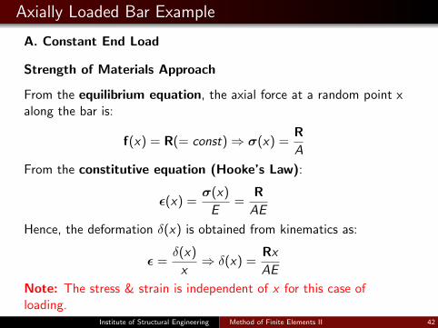
A. Constant End Load
Strength of Materials Approach
From the equilibrium equation, the axial force at a random point xalong the bar is:
f(x) = R(= const)⇒ σ(x) =R
A
From the constitutive equation (Hooke’s Law):
ε(x) =σ(x)
E=
R
AE
Hence, the deformation δ(x) is obtained from kinematics as:
ε =δ(x)
x⇒ δ(x) =
Rx
AE
Note: The stress & strain is independent of x for this case ofloading.
Institute of Structural Engineering Method of Finite Elements II 42
Axially Loaded Bar Example
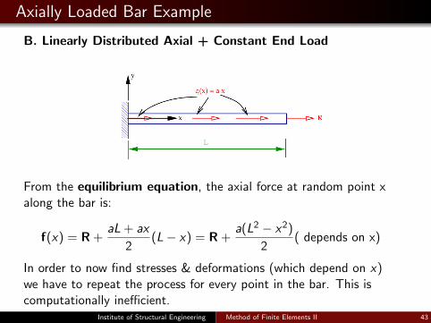
B. Linearly Distributed Axial + Constant End Load
From the equilibrium equation, the axial force at random point xalong the bar is:
f(x) = R +aL + ax
2(L− x) = R +
a(L2 − x2)
2( depends on x)
In order to now find stresses & deformations (which depend on x)we have to repeat the process for every point in the bar. This iscomputationally inefficient.
Institute of Structural Engineering Method of Finite Elements II 43
Axially Loaded Bar Example
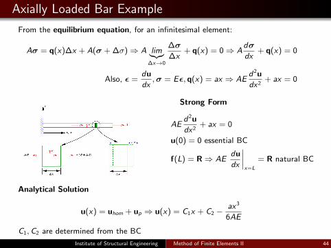
From the equilibrium equation, for an infinitesimal element:
Aσ = q(x)∆x + A(σ + ∆σ)⇒ A lim︸︷︷︸∆x→0
∆σ
∆x+ q(x) = 0⇒ A
dσ
dx+ q(x) = 0
Also, ε =du
dx,σ = Eε, q(x) = ax ⇒ AE
d2u
dx2+ ax = 0
Strong Form
AEd2u
dx2+ ax = 0
u(0) = 0 essential BC
f(L) = R⇒ AEdu
dx
∣∣∣∣x=L
= R natural BC
Analytical Solution
u(x) = uhom + up ⇒ u(x) = C1x + C2 −ax3
6AE
C1,C2 are determined from the BC
Institute of Structural Engineering Method of Finite Elements II 44
Axially Loaded Bar Example
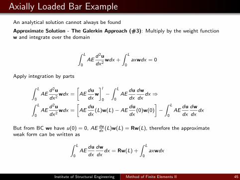
An analytical solution cannot always be found
Approximate Solution - The Galerkin Approach (#3): Multiply by the weight functionw and integrate over the domain
∫ L
0AE
d2u
dx2wdx +
∫ L
0axwdx = 0
Apply integration by parts
∫ L
0AE
d2u
dx2wdx =
[AE
du
dxw
]l0
−∫ L
0AE
du
dx
dw
dxdx ⇒∫ L
0AE
d2u
dx2wdx =
[AE
du
dx(L)w(L)− AE
du
dx(0)w(0)
]−∫ L
0AE
du
dx
dw
dxdx
But from BC we have u(0) = 0, AE dudx
(L)w(L) = Rw(L), therefore the approximateweak form can be written as∫ L
0AE
du
dx
dw
dxdx = Rw(L) +
∫ L
0axwdx
Institute of Structural Engineering Method of Finite Elements II 45
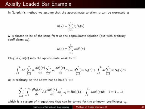
Axially Loaded Bar Example
In Galerkin’s method we assume that the approximate solution, u can be expressed as
u(x) =n∑
j=1
ujNj (x)
w is chosen to be of the same form as the approximate solution (but with arbitrarycoefficients wi ),
w(x) =n∑
i=1
wiNi (x)
Plug u(x),w(x) into the approximate weak form:
∫ L
0AE
n∑j=1
ujdNj (x)
dx
n∑i=1
widNi (x)
dxdx = R
n∑i=1
wiNi (L) +
∫ L
0ax
n∑i=1
wiNi (x)dx
wi is arbitrary, so the above has to hold ∀ wi :
n∑j=1
[∫ L
0
dNj (x)
dxAE
dNi (x)
dxdx
]uj = RNi (L) +
∫ L
0axNi (x)dx i = 1 . . . n
which is a system of n equations that can be solved for the unknown coefficients uj .
Institute of Structural Engineering Method of Finite Elements II 46
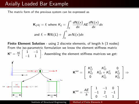
Axially Loaded Bar Example
The matrix form of the previous system can be expressed as
Kijuj = fi where Kij =
∫ L
0
dNj(x)
dxAE
dNi (x)
dxdx
and fi = RNi (L) +
∫ L
0
axNi (x)dx
Finite Element Solution - using 2 discrete elements, of length h (3 nodes)From the iso-parametric formulation we know the element stiffness matrix
Ke = AEh
[1 −1−1 1
]. Assembling the element stiffness matrices we get:
Ktot =
K e11 K 1
12 0K 1
12 K 122 + K 2
11 K 212
0 K 212 K 2
22
⇒
Ktot =AE
h
1 −1 0−1 2 −10 −1 1
Institute of Structural Engineering Method of Finite Elements II 47
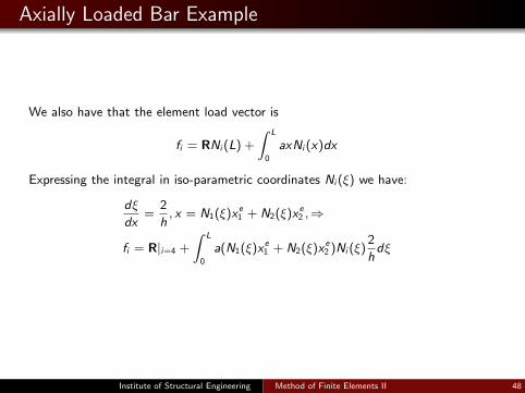
Axially Loaded Bar Example
We also have that the element load vector is
fi = RNi (L) +
∫ L
0
axNi (x)dx
Expressing the integral in iso-parametric coordinates Ni (ξ) we have:
dξ
dx=
2
h, x = N1(ξ)xe
1 + N2(ξ)xe2 ,⇒
fi = R|i=4 +
∫ L
0
a(N1(ξ)xe1 + N2(ξ)xe
2 )Ni (ξ)2
hdξ
Institute of Structural Engineering Method of Finite Elements II 48
Axially Loaded Bar Example
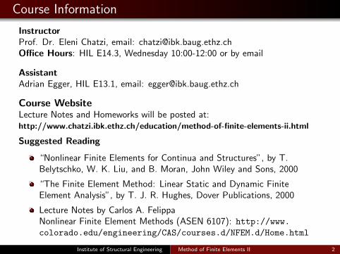
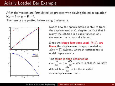
After the vectors are formulated we proceed with solving the main equationKu = f ⇒ u = K−1f.The results are plotted below using 3 elements:
Notice how the approximation is able to trackthe displacement u(x), despite the fact that inreality the solution is a cubic function of x(remember the analytical solution).
Since the shape functions used, Ni (x), arelinear the displacement is approximated as:u(x) =
∑i Ni (x)ui , where ui corresponds to
nodal displacements.
The strain is then obtained as
ε =du
dx⇒ ε =
dN
dxui where in slide 25 we have
defined B =dN
dxto be the so-called
strain-displacement matrix.
Institute of Structural Engineering Method of Finite Elements II 49