The federal funds market, excess reserves, and

unconventional monetary policy

by

Jochen H. F. GÜNTNER*)

Working Paper No. 1312 September 2013

DDEEPPAARRTTMMEENNTT OOFF EECCOONNOOMMIICCSS

JJOOHHAANNNNEESS KKEEPPLLEERR UUNNIIVVEERRSSIITTYY OOFF

LLIINNZZ

Johannes Kepler University of Linz Department of Economics

Altenberger Strasse 69 A-4040 Linz - Auhof, Austria

www.econ.jku.at

jochen.guentner@jku.at phone +43 (0)70 2468 -8360, -9679 (fax)

The federal funds market, excess reserves, and unconventional

monetary policy✯

Jochen H. F. Guntner❸

Johannes Kepler University Linz

First version: November 9, 2011

This version: September 16, 2013

Abstract

Following the bankruptcy of Lehman Brothers, interbank borrowing and lending dropped,

whereas reserve holdings of depository institutions skyrocketed, as the Fed injected liquidity

into the U.S. banking sector. This paper introduces bank liquidity risk and limited market

participation into a real business cycle model with ex ante identical financial intermediaries

and shows, in an analytically tractable way, how interbank trade and excess reserves emerge

in general equilibrium. Investigating the role of the federal funds market and unconventional

monetary policy for the propagation of aggregate real and financial shocks, I find that federal

funds market participation is irrelevant in response to standard supply and demand shocks,

whereas it matters for “uncertainty shocks”, i.e. mean-preserving spreads in the cross-section

of liquidity risk. Liquidity injections by the central bank can absorb the effects of financial

shocks on the real economy, although excess reserves might increase and federal funds might

be crowded out, as a side effect.

Keywords: Excess reserves; Federal funds market; Financial frictions; Liquidity risk; Unconventional monetary

policy

JEL Classification: C61; E32; E51; E52

✯I would like to thank Elena Afanasyeva, Rudiger Bachmann, Benjamin Born, Dirk Bethmann, Christiane Clemens,Christopher House, Johannes Pfeifer, Johann Scharler, Ajay Shenoy, and Henning Weber for helpful comments. Part of theresearch on this topic was conducted while the author visited the University of Michigan, Ann Arbor. Financial supportby the German Academic Exchange Service (DAAD) is gratefully acknowledged.

❸Jochen Guntner is Assistant Professor at the Department of Economics, Johannes Kepler University Linz. Address:Altenberger Strasse 69, 4040 Linz-Auhof, Austria. E-mail: jochen.guentner@jku.at, telephone: +43 732 2468-8360, fax:+43 732 2468-9679.

1 Introduction

Following the bankruptcy of Lehman Brothers, the Federal Reserve injected substantial amounts

of liquidity into the U.S. banking sector in order to contain tensions in the federal funds market.

As a result, the reserve holdings of depository institutions skyrocketed. Pundits have taken this

as a signal of ineffectiveness of the Fed’s liquidity facilities in promoting the supply of credit to

the economy (compare Keister and McAndrews, 2009). Figure 1 illustrates that excess reserves

used to play only a negligible role on the balance sheets of financial intermediaries throughout

the post-war period, averaging less than 0.05% of total deposits before September 2008.1 After

Lehman, excess reserves increased from virtually zero to almost 20%, whereas interbank lending,

i.e. federal funds and reverse repurchase agreements of U.S. commercial banks with other banks,

dropped from 5.5% to less than 1.5% as a fraction of total deposits.2

< Include Figure 1 about here >Identifying federal funds transactions based on Fedwire data, Ashcraft et al. (2011) document a

dramatic increase in bank liquidity risk in August 2007, due to looming intraday payments for

asset-backed commercial paper liquidity lines, whereas concerns about increased counterparty

risk in interbank transactions were largely irrelevant until October 2008. Likewise, Afonso and

Lagos (2012) show that the average number of daily trades and counterparties dropped from

above 860 to about 240 and from 4.5 to 3, respectively, whereas average loan size doubled during

the financial crisis of 2007–2009. Hence, the drop in the total volume of federal funds since 2008

was driven by a reduction in trade frequency rather than in trade size.

The aim of this paper is to show, in an analytically tractable way, how interbank lending and

excess reserves can emerge in general equilibrium. For this purpose, I introduce liquidity risk

in the spirit of Rochet and Tirole (1996) and Holmstrom and Tirole (1998) and limited federal

funds market participation in an otherwise frictionless real business cycle (RBC) model with

financial intermediation. The model can thus capture the prevalence of interbank credit before

as well as the rise in reserves during the “Great Recession” and is used to investigate the role of

the federal funds market and unconventional monetary policy for the propagation of aggregate

real and financial shocks.

In the model, interbank borrowing and lending arises from idiosyncratic uncertainty of ex ante

identical financial intermediaries. Building on Dib (2010), banks extend commercial loans to

1Aggregate excess reserves are defined as total minus required reserves of all depository institutions. All dataare from the Board of Governors of the Federal Reserve and seasonally adjusted.

2Throughout the paper, I use the terms “federal funds” and “interbank loans” interchangeably, when referringto unsecured short-term credit between financial intermediaries.

1

goods-producing firms according to a Leontief technology, i.e., they must simultaneously fulfill

a non-negativity constraint on liquidity and a minimum capital requirement, as in the Basel

accords. Deposits are stochastic at the bank level and realize only after a bank has chosen its

desired volume of loans and bank capital. Each individual bank is thus subject to liquidity risk

and an occasionally binding liquidity constraint. Institutions with low (high) deposit realizations

relative to their bank capital stock can engage in interbank borrowing (lending). Whether a

given bank participates in the federal funds market is exogenous, however. I abstract from

pro-cyclical balance sheet constraints in financial intermediation. Hence, my model represents

a complement rather than a substitute for the well-known “financial accelerator”.

Extending the approach in Wen (2011), I aggregate the occasionally binding liquidity constraints

of individual banks by assuming a suitable distribution function of their idiosyncratic deposit

realizations. The model can thus capture microeconomic uncertainty at the bank level even in

a loglinear approximation around the steady state.

With full participation in the federal funds market, interbank borrowing and lending provides

perfect insurance against liquidity risk. Accordingly, the banking sector is “self-sufficient” in the

sense of Holmstrom and Tirole (1998), attaining an optimal equilibrium allocation of liquidity.

Limited participation induces banks to hold excess reserves, raises the interest rate spread in

financial intermediation, and impairs thus steady-state real economic activity through a credit

cost channel (compare Kiyotaki and Moore, 2008).

Given a symmetric distribution function of deposit realizations and an exogenous, in particular

acyclical, participation in the federal funds market, the latter is irrelevant for the propagation

of conventional supply and demand shocks. On the contrary, the federal funds market is crucial

for attenuating “uncertainty shocks”, i.e. changes in the variance of banks’ deposit realizations.

An exogenous decrease in participation triggers a simultaneous increase in excess reserves and

an economic recession.

Unconventional monetary policy, modeled here as a liquidity injection by the central bank, can

reduce banks’ liquidity risk and stabilize real economic activity in response to financial shocks.

Depending on its implementation, however, it might lead to an even more pronounced increase

in excess reserves and a crowding out of interbank credit.

My work is most closely related to Gertler and Kiyotaki (2011). In their model, a continuum of

financial intermediaries is located on a continuum of islands. Each period, a fraction of firms is

randomly assigned the possibility to invest (compare also Kiyotaki and Moore, 2008). Financial

intermediaries can only lend to firms on the same island but to intermediaries on all islands.

Asymmetric information implies endogenous borrowing constraints both in the “retail” market

2

for deposits and the “wholesale” market for interbank credit.

Assuming a normal distribution of the stochastic deposit realizations (see, e.g., Frost, 1971),

idiosyncratic uncertainty in my model is, at the same time, less complex and more general than

in Gertler and Kiyotaki (2011). (i) Aggregate interbank credit, excess reserves, and commercial

loans have an analytical solution. (ii) The functional form assumption facilitates uncertainty

shocks, i.e. mean-preserving spreads in the distribution of liquidity shocks (see also Williamson,

1987). (iii) Given the focus on bank reserves and the federal funds market, in the present paper,

“unconventional monetary policy” refers to the Fed’s liquidity facilities rather than the direct

intermediation of credit by the central bank, as in Gertler and Karadi (2011).

The model in this paper bridges a gap in the literature on business cycles and financial frictions.

Excess reserves cannot be captured in a deterministic framework, where profit-maximizing banks

hold zero reserves except for legal requirements. When subject to uncertain in- and outflows of

liquidity, however, it is rational for individual banks to insure against negative liquidity shocks

by holding precautionary reserves. In the presence of protection against liquidity risk, in turn,

reserves become irrelevant (compare Poole, 1968). Numerous microeconomic contributions show

that a frictionless interbank market provides perfect insurance by pooling independent liquidity

risks (see, e.g., Bhattacharya and Fulghieri, 1994; Freixas et al., 2000).

Until recently, financial frictions in macroeconomics were mostly confined to the limited access of

firms to external finance, arising from asymmetric information between financial intermediaries

and ultimate borrowers (see, e.g., Williamson, 1987; Bernanke and Gertler, 1989).3 However, the

financial crisis of 2007–2009 originated from frictions within the banking sector, before spreading

to the real economy (compare Brunnermeier, 2009, and Woodford, 2010). Nevertheless, only a

small strand of the macroeconomic literature considers the effects of changes in credit conditions

that are unrelated to borrower characteristics, as in Cook (1999), Gertler and Kiyotaki (2011),

and Gertler and Karadi (2011).

Few macroeconomic models are able to generate excess reserves. If so, reserves are assumed to

be an input into a neoclassical production function for transaction services (see, e.g., Chari et al.,

1995; Christiano et al., 2010).4 Interbank borrowing and lending merely occurs between banks

that differ in their structural parameters, as in Dib (2010) and Gerali et al. (2010). While some

authors refer to these transactions as “federal funds”, financial intermediation is effectively split

3An extensive literature documents the quantitative importance of the financial accelerator in accounting forbusiness cycle fluctuations, both theoretically (see, e.g., Carlstrom and Fuerst, 1997; Bernanke et al., 1999) andempirically (see, e.g., Christensen and Dib, 2008).

4Chari et al. (1995) acknowledge that, dropping the production function for demand deposits, the nonegativityconstraint on excess reserves would hold with strict equality. In Christiano et al. (2010), reserves are explicitlyincluded into the production of liquidity services “as a reduced form way to capture the precautionary motive ofa bank concerned about [...] unexpected withdrawals”.

3

up into the collection of deposits and the provision of loans. Different rates of time preference

of depository and lending institutions thus facilitate a one-way stream of interbank credit from

patient to impatient, i.e. “between” ex ante heterogeneous financial intermediaries.

The rest of the paper is organized as follows. Section 2 describes the model’s timing and agents,

derives their individual decision rules and the aggregate equilibrium conditions. The calibration

of parameters and benchmark steady-state values are presented in section 3. Sections 4 and 5

illustrate the dynamic implications of federal funds trade and unconventional monetary policy,

respectively. Finally, I relate the model’s theoretical predictions to the response of the Fed to

the recent financial crisis and discuss the implications for monetary policy. Section 6 concludes.

2 The Model

The model is set up in infinite discrete time and comprises five types of economic agents: A

representative worker household, a representative banker household, a representative capital

goods producer, a representative entrepreneur and final goods producer, and a decentralized

banking sector.

The worker household enters each period with a predetermined level of bank deposits, supplies

homogeneous labor services and receives shareholder dividends from the final goods-producing

firm. Household income is either consumed or saved for subsequent periods in terms of bank

deposits, which yield a riskless real rate of return.

The banker household does not work, derives utility from consumption, and accumulates bank

capital, which is then provided to financial intermediaries. As in Dib (2010), bank capital or

equity pays a state-contingent real rate of return (dividend). I abstract from agency problems

between households and financial intermediaries.

The banking sector provides financial intermediation between lenders and borrowers by con-

verting household deposits into loans to entrepreneurs. Ultimate savers cannot lend directly

to ultimate borrowers at a single common interest rate – a feature of many pre-crisis models

criticized by Woodford (2010). Banks must satisfy a stylized minimum capital requirement

mimicking Basel II in order to lend to non-financial corporations. When choosing an optimal

level of bank capital, each bank knows the value of aggregate household deposits but does not

know its idiosyncratic deposit realization. Once the bank-specific liquidity shocks have occurred,

financial institutions might borrow or lend in an interbank market.5

5The liquidity shocks could equivalently be modeled in terms of stochastic deposit in- and outflows. Sinceone bank’s outflow is usually another bank’s inflow (compare Kaufman and Lombda, 1980), the correspondingprobability distribution would reasonably be mean zero. More generally, the uncertainty in this model shouldbe thought of as short-term funding uncertainty. Another possibility would be to introduce uncertainty aboutbanks’ investment opportunities, i.e. on the asset side, as in Gertler and Karadi (2011).

4

Entrepreneurs cannot accumulate own net worth and rely on external finance in order to acquire

the capital stock in advance of production. When the physical capital stock becomes productive

in the subsequent period, the representative entrepreneur hires labor services from the worker

household. After production, the depreciated capital is sold back to capital goods producers

and the bank loan is repaid. Any profits or losses are distributed to the firm’s shareholders –

the worker household. The representative capital goods producer recycles the predetermined

depreciated capital stock and invests, before selling the new productive capital to entrepreneurs.

2.1 The Banking Sector

A unit-mass continuum of ex-ante identical banks is indexed on the interval [0,1]. Banks enter

each period with zero assets and zero liabilities. Similar to Dib (2010), banks use a common

Leontief production function for providing loans. On the one hand, each bank i must satisfy

a stylized capital requirement by holding bank capital zt(i). On the other hand, lending to

entrepreneurs is bounded above by the bank’s disposable liquidity:

lt(i) =min{κzt(i), dt(i) + bt(i) + zt(i)} , (1)

where κ denotes the maximum admissible bank loans per unit of bank capital, i.e. the inverse of

the minimum bank capital ratio specified in the Basel II accord. Each period, bank i is subject

to a stochastic deposit realization, dt(i), that is i.i.d. across banks and through time. bt(i)denotes federal funds borrowing or lending of bank i.

The strict complementarity between the arguments in the Leontief production function should

not be taken literally, but serves as a modeling device to approximate the timing of liquidity

shocks in a three-period agency model (see, e.g., Rochet and Tirole, 1996). Suppose, e.g., that

the market for bank capital opens before the market for deposits, or that intermediaries are

subject to stochastic deposit in- and outflows throughout the period. As a consequence, banks

must commit to one input in (1) without knowing the quantity of the other input.

After zt(i) has been chosen, the idiosyncratic deposit shocks occur and each bank learns its

dt(i). Following a high (low) deposit realization relative to its stock of capital, bank i can lend

(borrow) in an interbank market, which facilitates the reallocation of liquidity between financial

intermediaries – a crucial characteristic of the U.S. federal funds market (see, e.g., Keister and

McAndrews, 2009; Afonso and Lagos, 2012). In the model, bt(i) represents uncollateralized

short-term borrowing (if bt(i) > 0) and lending (if bt(i) < 0) between financial intermediaries.

For these reasons, the terms “interbank market” and “federal funds market” are used inter-

changeably in this paper. The maximum disposable funds bank i can lend to entrepreneurs

5

thus amount to dt(i) + bt(i) + zt(i).At this point, I deliberately omit alternative ways of raising liquidity, after individual uncertainty

is resolved, such as the discount window, for example. Saunders and Urich (1988), Peristiani

(1998), and Furfine (2001) provide empirical evidence that banks are reluctant to borrow from

the discount window in “normal” times, fearing that the Federal Reserve and other financial

institutions might interpret this as a signal of poor liquidity management or financial distress.

Ennis and Weinberg (2013) study a theoretical model of the stigma attached to discount window

borrowing.

Suppose that bank i expects a volume Etdt(i) of deposits in period t, whereas its actual realiza-

tion, dt(i), deviates from this expectation with known exogenous variance, σ2t .

6 The uncertainty

in my model is thus purely idiosyncratic. In contrast to Holmstrom and Tirole (1998), I omit

the case, where all banks experience the same liquidity shock.7 Based on the incomplete infor-

mation about its available liquidity, bank i chooses an optimal level of zt(i) in order to maximize

expected profits in period t + 1,

Etπbt+1(i) ∶= (1 + rL

t )Etlt(i) + (1 + rRt )Etrrt(i) − (1 + rD

t )Etdt(i)−(1 + rB

t )Etbt(i) − (1 +EtrZt+1) zt(i), (2)

subject to the balance sheet identity,

lt(i) + rrt(i) ≡ dt(i) + bt(i) + zt(i), (3)

and a nonnegativity constraint on its liquid reserves,

rrt(i) ≥ 0. (4)

In (2), rLt , rR

t , rDt , and rB

t denote the real rates of return on bank loans, liquid reserves,

bank deposits, and federal funds, respectively, while rZt denotes the state-contingent return

on equity. As in Ashcraft et al. (2011), banks are not required to hold reserves. In practice,

required reserves correspond to a constant fraction of deposits and contributed very little to the

recent increase in total reserve balances.

6For concreteness, I assume that the probability distribution of dt(i) is sufficiently described by its first andsecond moment.

7In the data, there is no evidence of an aggregate run on banks by depositors. For the same reason, Ido not introduce an agency problem between financial intermediaries and depositors, as in Gertler and Karadi(2011). Due to the fact that the Leontief technology allows for “partial liquidation” of investment projects atthe individual bank level, the consequences of aggregate uncertainty would be less dramatic than in Rochet andTirole (1996) and Holmstrom and Tirole (1998), where negative excess liquidity leads to a termination of projectsand the productive sector’s ex post value goes to zero.

6

Substituting for Etrrt(i) from (3), expected profits of bank i simplify to

Etπbt+1(i) ∶= (rL

t − rRt )Etlt(i) − (rD

t − rRt )Etdt − (rB

t − rRt )Etbt(i) − (rZ

t − rRt )zt(i).

Note that I abstract from the issue of default in any of the banks’ assets or liabilities. It

is straightforward to account for the failure of bank loans to entrepreneurs by introducing a

productivity shock that represents the fraction of non-defaulting loans in equation (1). An

exogenous reduction in its cross-sectional expectation would then induce banks to raise rLt ,

whereas the conclusions in the present paper would not be affected.

2.2 The Household Sector

2.2.1 Workers

The infinitely-lived representative worker derives positive utility from consumption, Cwt , of the

final good and negative utility from hours spent working in goods production, Nt. Labor services

are rewarded with a real wage rate of wt. Consumption can be transferred across periods by

means of bank deposits, Dt, which yield a riskless rate of return rDt . Note that Dt ≡ ∫ 1

0 dt(i)di

and that Dt is a decision variable of the representative worker household, whereas the fraction

of deposits transferred to bank i is stochastic.

The worker chooses {Cwt ,Nt,Dt} to maximize expected discounted lifetime utility,

Et

∞∑ν=0

(βw)ν {ζt+ν lnCwt+ν − a

N1+γt+ν

1 + γ} , (5)

subject to the budget constraint in period t,

Cwt +Dt ≤ wtNt + (1 + rD

t−1)Dt−1 + πet , (6)

where πet are dividend payments received from goods producers. βw denotes the worker’s sub-

jective discount factor, γ the inverse Frisch elasticity of labor supply, and a a scaling parameter.

ln (ζt) = ρζ ln (ζt−1) + εζt is an autocorrelated consumption preference shock.

The corresponding first order conditions (FOCs) with respect to Cwt , Nt, and Dt are:

Cwt ∶ λw

t Cwt = ζt, (7)

Nt ∶ λwt wt = a (Nt)γ , (8)

Dt ∶ λwt = βwEtλ

wt+1 (1 + rD

t ) , (9)

where λwt is the Lagrange multiplier of the budget constraint. Equations (6), (7), (8), and (9)

represent the worker household’s equilibrium conditions.

7

2.2.2 Bankers

The infinitely-lived representative banker has zero labor endowment, derives utility from con-

sumption of the final good, Cbt , and accumulates bank capital, Zt. Household income arises from

the state-contingent return (dividend) rZt on bank capital as well as from any residual profits in

the banking sector. Note that Zt ≡ ∫ 10 zt(i)di and that the fraction of bank capital received by

bank i, zt(i), is assumed to be non-stochastic in order to keep financial intermediation tractable.

The banker chooses {Cbt , Zt} to maximize expected discounted lifetime utility,

Et

∞∑ν=0

(βb)ν {ζt+ν lnCbt+ν} , (10)

subject to the budget constraint in period t,

Cbt +Zt ≤ (1 + rZ

t )Zt−1 + πbt , (11)

where πbt denotes aggregate banking sector profits, and βb is the banker’s subjective discount

factor. The remaining parameters in the utility function and the consumption preference shock

are identical to those in (5). In the absence of inflation, the real stock of bank capital does not

depreciate over time, when used by banks.

The banker household’s FOCs with respect to Cbt and Zt are:

Cbt ∶ λb

tCbt = ζt, (12)

Zt ∶ λbt = βbEt [λb

t+1 (1 + rZt+1)] , (13)

where λbt is the Lagrange multiplier of the corresponding budget constraint. Equations (11),

(12), and (13) represent the banker’s equilibrium conditions.

The main motivation for modeling a separate banker household is to have some leeway in

the calibration of interest rates. Comparing equations (9) and (13), it is obvious that the

simultaneous accumulation of deposits and bank capital by a single worker-banker household

implies identical interest rates on Dt and Zt in equilibrium, up to first order. Setting βb < βw

facilitates a quantitatively relevant spread between the interest rates on deposits and bank

loans.8 Alternatively, I could assume that a strictly positive share of loans defaults in the

aggregate and that banks demand a risk premium on lt(i).8Note that my qualitative results do not depend on the assumption of a less patient banker household and

would persist for βb = βw. Alternatively, one could assume that financial intermediaries can divert a fraction ofbank capital, as in Dib (2010), effectively introducing default on bank capital.

8

2.3 The Production Sector

2.3.1 Capital Goods

After production in period t, a representative capital goods producer buys the depreciated

capital stock, (1− δ)Kt−1, and chooses optimal investment activity, It, to maximize the present

value of expected future discounted profits in terms of the worker’s utility,

Et

∞∑ν=0

(βw)ν λwt+ν {qt+ν [(1 − δ)Kt−1+ν + It+ν] − It+ν − qt+ν(1 − δ)Kt−1+ν}= Et

∞∑ν=0

(βw)ν λwt+ν {qt+νIt+ν − It+ν} , (14)

subject to the equation of motion of the aggregate capital stock:

Kt = (1 − δ)Kt−1 + It. (15)

The equality in (14) results from the assumption that the capital goods producer acquires

the depreciated and sells the new capital stock at the same real price of capital, qt+ν . As a

consequence, she never realizes any capital gains or losses. Perfect competition implies zero

profits in the capital goods-producing sector in each state of the economy.

The FOC with respect to investment and the equation of motion of the aggregate capital

stock determine the capital market equilibrium. In the absence of investment adjustment costs,

qt = 1,∀t.2.3.2 Final Goods

Entrepreneurs combine capital and labor services to produce a homogeneous final output good

according to the following Cobb-Douglas production function:

Yt = AtKαt−1N

1−αt , (16)

where ln (At) = ρA ln (At−1) + εAt represents a transitory total factor productivity (TFP) shock.

Note that the capital stock bought at the end of a period becomes productive in the subsequent

period, only. E.g., Kt−1 is predetermined in period t production.

The representative entrepreneur cannot accumulate own net worth and relies on external finance

in order to acquire the physical capital stock in advance of production. Similar to Gertler and

Kiyotaki (2011) and Gertler and Karadi (2011), there is no agency problem between the financial

intermediary and the firm. Accordingly, the real amount borrowed, Lt−1, equals the quantity

of productive capital in period t − 1:

Lt−1 =Kt−1. (17)

9

The entrepreneur chooses Kt−1 in period t − 1 and Nt in period t in order to maximize the

present value of expected future discounted profits in terms of the worker household’s utility,

Et

∞∑ν=0

(βw)ν λwt+ν {Yt+ν + (1 − δ)Kt−1+ν −wt+νNt+ν − (1 + rt−1+ν)Lt−1+ν} , (18)

where rLt is the real interest rate on a bank loan obtained at the end of period t.

Profit maximization requires that, up to first order, the expected real marginal return on the

capital stock used in production in t + 1 equals the real marginal cost per unit of Kt:

Et [rkt+1 + (1 − δ)] = 1 + rt, (19)

where rKt denotes the marginal product of capital, i.e.,

rKt Kt−1 = αYt. (20)

The FOC with respect to labor input in period-t production is given by

wtNt = (1 − α)Yt. (21)

2.4 Equilibrium in the Federal Funds Market

Recall that the banking sector has unit mass. Hence, expected deposits of each individual

bank, Etdt(i), equal aggregate deposits Dt and, similarly, zt(i) = Zt ∀i. The assumption of

homogeneous banks yields the following proposition.

Proposition 1 If banks are ex ante identical and share a common information set when making

their decisions, then each bank i expects the same Etdt(i) =Dt ≡ ∫ 10 dt(i)di and chooses the same

zt(i) = Zt ≡ ∫ 10 zt(i)di.

The proof of Proposition 1 corresponds to a straightforward symmetry argument. All banks

solve an identical optimization problem under idiosyncratic uncertainty.

Suppose further that, after the stochastic deposit inflows, bank i may access the federal funds

market with an exogenous probability ξt a la Calvo (1983), regardless of its dt(i).9 Ignoring

transaction costs, interbank borrowing and lending is strictly preferable to “financial autarky”

at any interest rate rBt ∈ (rR

t , rLt ), i.e., interest payments on reserve balances set a lower bound

to the federal funds rate (compare Ennis and Keister, 2008; Keister and McAndrews, 2009;

Bech and Klee, 2011).10

9Limited market participation can arise from private information about idiosyncratic liquidity shocks, as inHellwig (1994) and von Thadden (1997), or from an agency problem along the lines of Gertler and Kiyotaki(2011), which allows banks to divert interbank credit and prevents perfect liquidity insurance. Although asym-metric access to the interbank market, i.e. ξt conditional on dt(i), seems more realistic, symmetry is a commonassumption (see Gertler and Kiyotaki, 2011).

10In reality, banks in need of liquidity can borrow from the Fed through the discount window. The interestrate interval is therefore bounded above by min {rL

t , rDW

t }, where rDW

t is the cost associated with borrowing at

10

If ξt = 0, each bank i is stuck with its bank capital Zt and its deposit realization dt(i). Its

lending to entrepreneurs is thus bounded above by the minimum of its leveraged capital and

loanable funds, i.e. lt(i) = min{κZt, dt(i) +Zt}, while its excess liquidity amounts to rrt(i) =max{dt(i) − (κ − 1)Zt,0}.If ξt = 1, the federal funds market allows banks with a high deposit realization to lend excess

liquidity and banks with a low realization to narrow their liquidity gap, effectively reallocating

funds to their most productive use (compare Keister and McAndrews, 2009). While actual lend-

ing to entrepreneurs derives from the Leontief technology in (1), bank-specific excess liquidity

amounts to a smaller residual than in isolation:

rrt(i) =max{dt(i) + bt(i) − (κ − 1)Zt,0} . (22)

Now consider bank i immediately after its idiosyncratic deposit realization:

Case 1: If dt(i) ≤ (κ − 1)Zt, the bank is a potential borrower in the federal funds market. For

rBt ∈ (rR

t , rLt ), it will demand exactly the amount of federal funds necessary to close its liquidity

gap, (κ − 1)Zt − dt(i). As a consequence, the rationing argument in lending to entrepreneurs is

bank i’s disposable liquidity, lt(i) = dt(i) + bt(i) +Zt, with

bt(i) =⎧⎪⎪⎪⎨⎪⎪⎪⎩(κ − 1)Zt − dt(i) ≥ 0 with probability ξt

0 with probability 1 − ξt

(23)

Case 2: If dt(i) > (κ − 1)Zt, bank i is a potential lender in the federal funds market and will

offer exactly its excess liquidity, dt(i)− (κ− 1)Zt, as long as the federal funds rate is within the

boundaries set by the interest paid on reserve balances and the rate earned on loans. In this

case, the minimum capital requirement represents the rationing argument in the bank’s Leontief

loan production function, i.e. lt(i) = κZt, and

bt(i) =⎧⎪⎪⎪⎨⎪⎪⎪⎩(κ − 1)Zt − dt(i) < 0 with probability ξt

0 with probability 1 − ξt

(24)

Note that, at a federal funds rate rBt < rR

t , it is profitable – even for a potential lender – to

borrow in the federal funds market and hold the proceeds as reserves in order to make a riskless

profit. The increased demand for federal funds should raise their price, i.e. the federal funds

rate, until rBt ≥ rR

t is satisfied again.

the discount window, including possible stigma effects. Bech and Klee (2011) develop a model of a segmentedinterbank market to explain the phenomenon that the effective federal funds rate has been below the interestrate paid on reserve balances in the U.S. since October 2008.

11

Similarly, rBt > rL

t implies that lending in the federal funds market is more profitable than

making loans to entrepreneurs. Even under the assumption that the banking sector as a whole

is a price taker in the market for bank loans and that Lt ≡ ∫ 10 lt(i)di has no effect on rL

t , the

increased supply of federal funds should depress the corresponding interest rate until rBt ≤ rL

t .

2.4.1 Federal Funds Market Clearing

Building on Wen (2011), who investigates input and output inventory dynamics using a Pareto

distribution, I assume a suitable functional form for the probability distribution of the stochas-

tic deposit realizations, dt(i). This facilitates aggregating the kinked equilibrium conditions of

individual banks for the banking sector as a whole.

Denote by f(dt(i)) and F (dt(i)) the probability density function (pdf ) and the cumulative dis-

tribution function (cdf ), respectively, of bank i’s stochastic deposit realization and suppose that

dt(i) is drawn from a time-varying normal distribution with mean Dt and standard deviation

σt, i.e. dt(i) ∼ N (Dt, σ2t ). For a continuum of financial firms, F (x) denotes both the ex ante

probability that the deposit realization of a given bank is below x and the ex post fraction of

banks with dt(i) ≤ x.

Federal funds market clearing requires that the supply of liquidity by potential lenders with

access to the interbank market equals the demand by potential borrowers. From (23) and (24),

it is straightforward to derive aggregate interbank borrowing and lending as the conditional ex-

pectation of bt(i) for the continuum of banks left and right of the cutoff, (κ−1)Zt, respectively.

Under the distributional assumptions for dt(i), aggregate demand for federal funds equals

Et [bt(i)∣dt(i) ≤ (κ − 1)Zt] = ξt {[(κ − 1)Zt −Dt]F ((κ − 1)Zt) + σ2t f((κ − 1)Zt)} ≥ 0, (25)

while aggregate supply of federal funds by banks with a high deposit realization equals

Et [bt(i)∣dt(i) > (κ − 1)Zt] = ξt {[(κ − 1)Zt −Dt] [1 − F ((κ − 1)Zt)] − σ2t f((κ − 1)Zt)} ≤ 0. (26)

The expressions in (25) and (26) yield the federal funds market clearing condition,

ξt {[(κ − 1)Zt −Dt]F ((κ − 1)Zt) + σ2t f((κ − 1)Zt)}

= ξt {[Dt − (κ − 1)Zt] [1 − F ((κ − 1)Zt)] + σ2t f((κ − 1)Zt)} , (27)

which implies the following important proposition.

Proposition 2 Assuming a symmetric probability distribution for the stochastic deposit real-

izations and symmetric access to the federal funds market, (κ − 1)Zt = Dt is necessary and

sufficient for an equilibrium in the federal funds market in period t.

12

Proof. See Appendix A. ∎The federal funds market clears, if and only if banks choose the effective level of bank capital,

κZt, in accordance with expected disposable funds (Dt + Zt), before idiosyncratic uncertainty

is resolved.

Note that the equilibrium condition in (27) is independent of the federal funds rate, rBt . The

symmetry assumptions in Proposition 2 imply that the federal funds rate is indeterminate, while

rBt ∈ (rR

t , rLt ). In order to pin down rB

t uniquely, further assumptions would be necessary.11

From (2), rBt matters for the distribution of profits across individual banks, whereas the total

volume of interbank borrowing and lending is fully determined by the f(dt(i)) and ξt. Since

the ex-post nonzero profits or losses of individual banks, πbt(i), are settled through the banker

household, the exact federal funds rate is irrelevant for the interest rate spread in financial

intermediation. Each bank i starts the subsequent period with zero net worth.12

This simplifying assumption also implies that, in normal times, monetary policy merely guar-

antees a federal funds rate satisfying rBt ∈ (rR

t , rLt ). A monetary extension of the model readily

accommodates a Taylor-type interest rate rule, where the central bank sets, e.g., rRt or the

interest rate on bank deposits, rDt ∈ (rR

t , rLt ).

2.4.2 Aggregate Lending and Excess Reserves

Given the distributional assumption about dt(i), we can furthermore aggregate the actual lend-

ing to entrepreneurs by individual banks. Recall that, for banks with a low deposit realization

relative to the predetermined amount of bank capital, lt(i) = dt(i) + bt(i) + Zt, whereas banks

with a high deposit realization lend lt(i) = κZt.

Corollary 1 Ex ante expected lending to entrepreneurs by each individual bank i and ex post

lending to entrepreneurs by the banking sector as a whole, Lt, are both given by

Etlt(i) = Lt = κZt − (1 − ξt) {[(κ − 1)Zt −Dt]F ((κ − 1)Zt) + σ2t f((κ − 1)Zt)} . (28)

Proof. See Appendix A. ∎Note from (28) that, in general, the total volume of loans, Lt, differs from the maximum volume

of loans facilitated by effective bank capital, κZt, implying Corollary 2.

Corollary 2 With idiosyncratic uncertainty about banks’ stochastic deposit realizations, aggre-

gate lending to entrepreneurs by the banking sector as a whole is bounded above by both arguments

11Bech and Klee (2011) model bilateral federal funds rates as bargaining outcomes between potential lendersand potential borrowers, reflecting their alternative options and respective bargaining power.

12In Gertler and Kiyotaki (2011), banks carry non-zero net worth across periods. In order to eliminatedifferences in net worth and ex ante expected rates of return between investing and non-investing islands, theyallow for arbitrage at the beginning of each period, temporarily breaking market segmentation.

13

of the Leontief loan production technology in (1), i.e.

Lt ≤min{κZt,Dt +Zt} , (29)

which holds with equality if and only if ξt = 1.

Proof. The proof follows directly from Proposition 2 (κZt =Dt +Zt) and Corollary 1:

Lt = κZt − (1 − ξt)σ2t f((κ − 1)Zt) = κZt − (1 − ξt)σ2

t f(Dt). ∎If ξt < 1, idiosyncratic deposit shocks cause an inefficient distribution of liquidity across banks.

Note that the financial frictions in this model are literally due to limited market participation.13

The federal funds market pools liquidity and helps to prevent a wasteful accumulation of deposits

in unconstrained financial intermediaries. Only if all banks have access to the federal funds

market, liquid reserves are fully drawn down and the maximum leverage ratio is exhausted,

while κt ≡ Lt

Zt≤ κ in general. In line with Holmstrom and Tirole (1998), ξt = 1 attains an

optimal reallocation of loanable funds.

Equation (22) implies that banks with a high deposit realization and no access to the federal

funds market end up holding liquidity. This corresponds to the excess reserves of bank i, in

the model. Although this treatment of excess reserves might seem somewhat unconventional, it

reflects the precautionary motive of banks. In the presence of positive opportunity costs, excess

reserves will be zero, unless liquidity shocks and frictions in the interbank market coincide, i.e.

σt > 0 and ξt < 1 (see, e.g., Ennis and Keister, 2008; Ashcraft et al., 2011; Ennis and Wolman,

2012). As pointed out by Kaufman and Lombra (1980), the observed level of excess reserves is

the result of stochastic deposit in- and outflows rather than the result of a desire of banks to

hold excess reserves. Finally, i.i.d. liquidity shocks and the Calvo probability of access to the

interbank market imply that the realizations of rrt(i) are also i.i.d. across banks and through

time. This is consistent with the empirical finding of substantial fluctuations in bank-specific

reserve balances from quarter to quarter (see Ennis and Wolman, 2012).

Aggregate excess reserves in the banking sector correspond to the conditional expectation of

(22) with a probability weight of (1 − ξt), i.e.

Etrrt(i) = Rt = (1 − ξt) {[(κ − 1)Zt −Dt] [1 − F ((κ − 1)Zt)] + σ2t f((κ − 1)Zt)} (30)

or, equivalently, Rt =Dt +Zt −Lt.

Corollary 3 If the federal funds market is in equilibrium, then aggregate excess reserves in the

banking sector are bounded below by 0 and bounded above by σ2t f((κ − 1)Zt).

13With a continuum of banks, ξt < 1 can also be interpreted as a restriction on the size of individual interbankloans in the presence of private information, as in Bhattacharya and Fulghieri (1994).

14

Proof. The proof follows immediately from equation (30) and Proposition 2:

Rt = (1 − ξt)σ2t f((κ − 1)Zt) = (1 − ξt)σ2

t f(Dt). ∎In the model, the total quantity of reserves is determined by the distribution of liquidity and the

interbank market friction, ξt. This implies that the demand curve for reserves is vertical, while

changes in demand are accommodated by the Fed, and seems to contradict the perception that

the total level of reserves in the banking system is determined almost exclusively by the central

bank (compare Keister and McAndrews, 2009). On the one hand, this reflects the reduced-form

approach to modeling liquidity shocks and the exogenous probability of access to the federal

funds market, and should hence be taken with a grain of salt. On the other hand, the European

Central Bank (ECB) provided unlimited credit at the policy rate through its fixed-rate tender

with full allotment (FRFA), starting in October 2008, thus effectively abandoning the control

of aggregate reserves outstanding. In section 5, I show how large reserve balances can arise as

a byproduct of unconventional monetary policy in the model, whereas Rt is (close to) zero in

normal times (see, e.g., Keister and McAndrews, 2009; Ennis and Wolman, 2012).

The banking sector is closed by assuming free entry into financial intermediation. Thus, expected

profits of individual banks and realized profits of the banking sector as a whole equal zero.

2.4.3 The Role of σt vs. ξt

At this point, it seems advisable to highlight the difference between the two time-varying param-

eters that determine the model’s financial friction. The standard deviation of individual banks’

stochastic deposit realizations, σt, represents the degree of idiosyncratic uncertainty in financial

intermediation. While rBt ∈ (rR

t , rLt ), “liquidity insurance” through the federal funds market is

strictly preferable to retaining excess reserves or bank capital. Accordingly, σt determines the

average bank’s demand for interbank borrowing and lending and, for a banking sector of mass

one, the aggregate demand for federal funds transactions.

For a given level of idiosyncratic uncertainty, ξt is the ex ante probability that bank i enters

the federal funds market, conditional on rBt ∈ (rR

t , rLt ). With a unit mass continuum of financial

intermediaries, ξt also equals the ex post fraction of banks with access to interbank borrowing

and lending. It determines thus the fraction of excess liquidity that banks with a high deposit

realization lend to banks with a low realization and is best understood as a measure of supply

in the federal funds market.

In short, σt determines the aggregate volume of excess liquidity, while ξt determines how this

is split between federal funds and excess reserves. Using the terminology of Afonso and Lagos

(2012), σt and ξt reflect the intensive margin and the extensive margin of interbank borrowing

15

and lending.

Figure C.1 in Appendix C illustrates the implications of ξt for aggregate lending to entrepreneurs

in terms of f(dt(i)). Consider panel (a) first. If ξt = 1, interbank borrowing and lending provides

perfect insurance against idiosyncratic deposit shocks. Each bank i attains the optimal level of

liquidity, dt(i) + bt(i) = (κ − 1)Zt, regardless of its realization dt(i). Corollary 1 implies that

Lt =Dt +Zt = κZt, in this case, while Rt =Dt +Zt −Lt = 0.

Consider now panel (b). If ξt < 1, only a fraction of all banks has access to the interbank market.

Accordingly, dt(i)+bt(i) ≠ (κ−1)Zt for some banks i, due to bt(i) = 0. For a unit-mass continuum

of banks, ξt can equivalently be interpreted as the share of each bank’s ∣dt(i)−(κ−1)Zt∣ that is

offset by borrowing or lending in the federal funds market (compare Bhattacharya and Fulghieri,

1994). In aggregate, this corresponds to the shaded area in panel (b), while aggregate excess

reserves correspond to the non-shaded area below f(dt(i)) right of the cutoff (κ− 1)Zt. In this

case, Lt <Dt +Zt = κZt and Rt > 0.

3 Calibration and Steady State

The model presented above is highly stylized in many dimensions. As it is therefore impossible

to match the empirical counterparts of all variables, the following calibration focuses on the

banking sector and, in particular, on aggregate excess reserves and the federal funds market.

3.1 Parameter Values

As far as possible, I choose standard parameter values in line with the RBC literature. The

worker household’s inverse Frisch elasticity of labor supply, γ, is set equal to 1. The weight of

labor in the utility function, a, is calibrated in order to obtain a steady-state employment equal

to 1/3 of the total time endowment.

Note that bankers are assumed to be less patient than workers. Their subjective discount factor,

βb, is set to .94, whereas βw = .995 for the worker household, implying a quarterly rate of time

preference of 6.4% and .5%, respectively. By setting the quarterly depreciation rate of physical

capital, δ, to .025 and the elasticity of final output with respect to capital, α, to 1/3, the capital-

and goods-producing sectors in my model are entirely standard.

I now turn to the calibration of the banking sector. In equation (1), κ represents the maximum

ratio of bank loans to bank capital. With regard to the Basel accords, I set κ to 12.5, implying a

minimum ratio of bank capital to entrepreneurial loans of 8%. In the presence of excess reserves,

1κt= Zt

Ltwill be higher than this regulatory minimum. Note also that this implies an aggregate

debt-to-equity ratio, Dt

Zt, of (κ − 1) = 11.5, in equilibrium.

16

Recall that σt and ξt denote the exogenous standard deviation of stochastic deposit realizations

and the Calvo probability of access to the federal funds market. In the benchmark calibration,

the corresponding stationary values, σ∗ and ξ∗, are set to 1, targeting the situation before the

crisis, when interbank lending was positive and excess reserves were virtually equal to zero.

< Include Table 1 about here >The dynamics of the general equilibrium model are driven by four stochastic processes. I assume

that innovations to goods production technology, consumer preferences, the variance of deposit

realizations, and participation in the federal funds market follow a first-order autoregressive

process in logs, i.e., ln(xt) = ρx ln(xt−1) + εxt , where ρx = .95 for x = A, ζ, σ, ξ. For convenience,

Table 1 summarizes the parameters determining the steady state.

3.2 Stationary Equilibrium

Abstracting from aggregate shocks, it is straightforward to solve for the stationary equilibrium.

Note that banks are subject to idiosyncratic uncertainty about their deposit realizations, even

in the absence of aggregate risk.

< Include Table 2 about here >The above calibration implies an annualized capital-output-ratio of 2.4. Consumption of the

worker and banker households account for 71.1 and 4.9%, respectively, while capital investment

accounts for the remaining 24% of total output.

Due to the fact that entrepreneurs require bank loans for purchasing the physical capital stock,

the aggregate loan-to-output ratio is identical to the capital-output ratio. Note that L∗ =D∗ + Z∗, if and only if all banks have access to the federal funds market, i.e. ξ∗ = 1, as in the

benchmark case. Hence, banks can perfectly insure against liquidity shocks by borrowing and

lending amongst each other.

A steady-state value of interbank borrowing, B∗∣dt(i)≤(κ−1)Z∗ , equal to 4.4% of aggregate deposits

and the absence of excess reserves in the steady state (R∗ = 0) were targeted by setting σ∗ = ξ∗ =1 in the benchmark calibration. These values are understood to be only suggestive. By setting

the maximum leverage ratio, κ, to 12.5, I ensure that the equity-to-loans ratio, Z∗

L∗matches the

minimum capital requirement of 8% stipulated in the Basel accords.

The quarterly interest rate on bank deposits, rD∗, is pinned down by the subjective time discount

rate of workers and invariant to the rest of the calibration. Similarly, bankers’ subjective time

discount rate determines the steady-state return on bank capital, rZ∗ = .0638. Free entry into

financial intermediation implies that banks make zero profit, on average, whereas each bank

17

i makes zero profit, if and only if ξ∗ = 1. In general, microeconomic uncertainty implies that

individual banks realize losses or gains, which are netted through the banker household at the

end of each period. Given the steady-state values of the other variables in equation (2), the

free-entry condition also determines the loan interest rate, rL∗ = .0097.

The user cost of capital comprises the loan rate and the quarterly depreciation rate. Assuming

perfect competition, this will be equal to the marginal product of capital, i.e. rK∗ = .0347 in

the benchmark steady state.

A ceteris paribus14 increase in the standard deviation of deposit realizations, σ∗, implies a higher

steady-state volume of federal funds, without affecting R∗ = 0. A ceteris paribus decrease in ξ∗

reduces banks’ participation in the interbank market and raises their holdings of excess reserves,

instead. As a consequence, the equity-to-loans ratio rises, signalling higher costs of financial

intermediation, which are passed on to entrepreneurs through an increase in the interest rate on

bank loans, rL∗. Accordingly, a decrease in ξ∗ impairs the efficiency of the banking sector. Note

that the debt-to-equity ratio, D∗

Z∗= 11.5, will not be affected. The set of steady-state values

obtained for the benchmark parameter calibration is summarized in Table 2.

4 Shocks to Financial Intermediation

This section discusses the implications of idiosyncratic uncertainty in financial intermediation

for the propagation of two novel shocks inherent in the banking sector. For the dynamic analysis,

the model is loglinearized around the non-stochastic steady state (see Appendix B) and impulse

response functions are computed for ξ∗ = 1, .5, and 0. While most variables’ steady state values

are broadly insensitive to ξ∗, B∗ and R∗ are equal to (σ∗)2f((κ − 1)Z∗) and 0 for ξ∗ = 1 and

vice versa for ξ∗ = 0, respectively. For ξ∗ = .5, half of all banks borrow or lend in the interbank

market. The liquidity risk (σ∗)2f((κ − 1)Z∗) is therefore split equally between federal funds

and excess reserves. For ease of interpretation, the impulse response functions of federal funds

and excess reserves are in terms of deviations from steady state as a fraction of steady-state

deposits, D∗.

The propagation of standard supply and demand shocks will not be discussed here, in detail.

Nevertheless, two comments are in order. First, the impulse responses of real variables to an

innovation in total factor productivity (TFP) and household preferences, respectively, are in line

with those obtained from a textbook RBC model. Second, ξ∗ is irrelevant for the propagation

of standard supply and demand shocks. In response to a positive TFP shock, e.g., the banking

sector’s aggregate balance sheet expands to accommodate higher loan demand by entrepreneurs.

14In particular, maintaining ξ∗ = 1 and thus unrestricted access to the federal funds market.

18

The assumption that σt follows an exogenous process implies that the uncertainty faced by each

bank i is independent of the size of its balance sheet. Accordingly, an expansion corresponds to

a rightward shift of f(dt(i)), or a variance-preserving increase in the mean. Similarly, a positive

preference shock induces a contraction of banks’ balance sheets and a leftward shift of f(dt(i)).The corresponding impulse response functions are available from the author.

4.1 Uncertainty Shocks

Borrowing from the terminology in Bloom (2009), I use the term “uncertainty shock” to describe

an exogenous change in the standard deviation of banks’ idiosyncratic deposit realizations. This

is adequate, as changes in σt represent second-order shocks, i.e. innovations in the variance of

dt(i) for a constant mean. Assuming a symmetric probability distribution, liquidity risk in this

model is inherently microeconomic, and should not be confounded with the growing literature

on macroeconomic volatility shocks (see, e.g., Fernandez-Villaverde et al., 2011).15

Figure 2 plots the impulse response functions to an unexpected transitory 10% increase in the

standard deviation of dt(i), i.e., σt jumps from 1 to 1.1. While this corresponds to a moderate

increase in the variance of dt(i) by 21%, the reported impulse responses are scalable by changing

the size of the shock, given the model’s loglinear approximation around the steady state.

< Include Figure 2 about here >Recall that the capital stock is acquired and installed one period in advance of production.

Therefore, shocks to financial intermediation affect the firm’s capacity with a lag of one quarter.

A temporary increase in σt implies that, on average, banks experience larger deviations from

Etdt(i) and have thus a stronger need for federal funds transactions. Otherwise, they end up

holding larger excess reserves.

Intuitively, this kind of uncertainty shock should not affect real economic activity, if access to

the federal funds market is complete. Figure 2 illustrates that, by borrowing from and lending

to each other, banks can perfectly insure against idiosyncratic uncertainty, regardless of σt, as

long as ξ∗ = 1. The volume of interbank borrowing and lending increases by .43% of steady-state

deposits, before converging back to its steady state, whereas none of the other variables deviates

from its stationary equilibrium.16 Thus, a frictionless federal funds market completely absorbs

uncertainty shocks.

15The deviations of all banks’ stochastic deposit realizations from the mean of the distribution average out,in each period. I assume that there is no uncertainty about the aggregate level of deposits, Dt.

16Note that a percentage deviation i. t. o. steady-state deposits, i.e. Bt−B∗

D∗, of .43% corresponds to a percentage

deviation from steady-state interbank borrowing, Bt−B∗

B∗= Bt−B

∗

D∗⋅ D

∗

B∗= .43 ⋅ 1

.0432, of 10%.

19

Consider now ξ∗ = .5, where bank’s liquidity risk is split equally between federal funds and excess

reserves, in the steady state. Even though both bank capital and deposits increase in response

to the σt-shock, aggregate lending to entrepreneurs decreases. The wedge between Dt +Zt and

Lt corresponds to the increase in excess reserves. Both Bt and Rt increase, if access to the

federal funds market is limited. While interbank borrowing and lending is costless, however,

higher reserves induce resource costs, which are passed on to entrepreneurs through the interest

rate on bank loans. The spread in financial intermediation increases, as the latter rises by more

than the interest rate on deposits.

From equation (19), an increase in the loan rate, rLt , must be offset by an equivalent increase in

the expected marginal product of the physical capital stock. With TFP unchanged, this implies

a reduction in Kt, which becomes productive as of period t+1. Accordingly, capital investment

drops, on impact, before recovering in the second quarter after the shock. Initially, the worker

household raises its labor supply, as the higher interest rate on bank deposits induces higher

savings, less consumption, and thus an increase in the marginal utility of consumption. The

additional labor input temporarily sustains the original output level.17

Once the downsized capital stock becomes productive, the economy enters into a recession. The

decrease in Kt reduces the marginal productivity of labor, both Nt and wt drop below their

steady-state values, and output falls short of its stationary equilibrium value by about 8 basis

points, before slowly recovering along with the capital stock and employment.

If ξ∗ = 0, the federal funds market is inoperative. As a consequence, banks with a high deposit

realization, dt(i) > (κ − 1)zt(i), maintain excess reserves, while banks with a low realization,

dt(i) < (κ − 1)zt(i), lack the liquidity to exhaust the minimum capital requirement and end up

withzt(i)lt(i)> 8%. The same frictions discussed in detail for ξ∗ = .5 occur to an extreme degree, in

this case. To be precise, the impulse responses to an uncertainty shock in terms of the deviations

from steady state are twice as large for ξ∗ = 0.

In terms of the model, the period before Lehman Brothers can be interpreted as a period of

pure uncertainty shocks, while 0 < ξt < 1. Ashcraft et al. (2011) find that both aggregate excess

reserves and aggregate federal funds transactions increased in August 2007, consistent with the

conditional comovement of Bt and Rt in the model.18

A frictionless interbank market allows banks to perfectly insure against idiosyncratic uncertainty

17Recall that the economy’s aggregate resource constraint deviates from the standard Yt = Ct + It. Instead,in this model, Yt = Cw

t + Cb

t + It + (Zt − Zt−1) + (Rt −Rt−1), i.e., changes in the stock of bank capital, Zt, or inaggregate excess reserves, Rt, absorb or release real resources, corresponding to a saving or storage technology.In the steady state, the resource constraint boils down to Y ∗ = C∗ + I∗, where C∗ = Cw∗ +Cb∗.

18Ashcraft et al. (2011) argue that, in response to the increase in liquidity risk, “constrained banks”, whichare not able to borrow in the federal funds market, could increase their holdings of precautionary excess reserves,whereas banks with the ability to borrow could tap the federal funds market as needed, i.e. σt ↑ for ξt = ξ∗ < 1.

20

as well as σt-shocks. The lower ξ∗, the larger is the share of all banks with either excess reserves

or excess bank capital. This impairs the efficiency of financial intermediation in the steady state

and, more importantly, the banking sector’s ability to absorb the effects of uncertainty shocks

on real economic activity.

4.2 Financial Friction Shocks

Consider now a temporary exogenous change in the fraction of financial institutions participating

in the federal funds market. Events of this kind are called “illiquidity waves” in Brunnermeier

(2009) or “liquidity crises” in Gertler and Kiyotaki (2011). Recall that idiosyncratic uncertainty

(σt > 0) induces a demand for liquidity insurance, whereas 0 ≤ ξt ≤ 1 determines the relative

prevalence of federal funds and excess reserves.

ξt captures all factors which might keep an individual bank away from the interbank market.

The model does not distinguish between voluntary autarky of potential lenders, e.g. due to

risk considerations or alternative lending opportunities, and involuntary exclusion of potential

borrowers from the market, e.g. due to selection. One interpretation for the exogenous change

in ξt is the deterioration of banks’ balance sheets following the bankruptcy of Lehman Brothers.

The resulting increase in the perceived or actual counterparty risk of interbank credit motivates

the voluntary absence of potential lenders and thus the above symmetry assumption.

Figure 3 depicts the impulse response functions of selected variables to a financial friction shock.

ξt drops by .1 before following an autoregressive process back to ξ∗, i.e., ten percent of the unit

mass of banks do not participate in the federal funds market, temporarily.19 As a consequence,

a larger fraction of banks ends up holding either excess reserves or excess capital, after realizing

an imbalance between dt(i) and (κ − 1)Zt.

< Include Figure 3 about here >In response to the shock, aggregate interbank borrowing drops by .43% of steady-state deposits,

whereas aggregate excess reserves increase by the same amount. Comparing impulse responses

with those in Figure 2, financial friction and uncertainty shocks have similar qualitative effects,

except for Bt and Rt, which deviate from their steady-state values in opposite directions.

The increase in excess reserves raises the spread between the interest rates on bank loans and

deposits. Higher costs of financial intermediation require an offsetting increase in the expected

marginal product of capital, i.e. a reduction in Kt, and thus a pronounced disinvestment in the

19Note that ξt is in percentage point rather than in % deviations from steady state in order to avoid an effectof ξ∗ on the size of the shock. Admissible values for ξt are from the interval [0,1]. Accordingly, impulse responsesfor ξ∗ = 0 are skipped in Figure 3, as a further deterioration of access to the federal funds market is impossible,in this case.

21

period of the shock. While the initial capital stock is still in use, production can only adjust

through employment. As in section 4.1, the higher interest rate on deposits induces the worker

household to save more, consume less, and expand its labor supply, which depresses the real

wage and sustains output, initially.

Once the downsized capital stock becomes productive, the economy enters into a recession.

Output and employment follow the same qualitative and quantitative patterns as in response

to a 10%-increase in σt for ξ∗ = 0. Now, however, the impulse responses are independent of ξ∗.

For a given liquidity risk, what matters is the change in the financial friction, i.e. the share of

banks that is “driven out of the federal funds market”, rather than its steady-state level.

In this model, uncertainty and financial friction shocks are distinguishable only by the responses

of federal funds and excess reserves. Both σt and ξt affect the spread in financial intermediation

and thus real economic activity in the same way. The impulse responses to a financial friction

shock are independent of ξ∗, as long as the steady-state participation in the federal funds market

is irrelevant for the size of the innovation.

The empirical findings in Afonso and Lagos (2012) suggest that the period after October 2008

corresponds to a period of coinciding uncertainty and financial friction shocks. Although average

trade size increased, which suggests a positive σt-shock, aggregate federal funds market volume

decreased and excess reserves rose dramatically, suggesting a negative ξt-shock. While the model

predicts that both shocks raise Rt, if ξt < 1, the overall impact on Bt is ambiguous.

5 Unconventional Monetary Policy

In the previous analysis, monetary policy is assumed to merely guarantee that the interest rate

on federal funds satisfies rBt ∈ (rR

t , rLt ).20 Central bank policy in “normal” times is commonly

described as implementing the desired monetary stance by targeting the federal funds rate. As

illustrated in Figure 1, the benchmark calibration (ξ∗ = 1) is consistent with the situation until

mid-2007, when excess reserves were virtually equal to zero. A monetary extension of the model

would readily accommodate a Taylor-type interest rate rule, where the central bank sets, e.g.,

rRt or the interest rate on bank deposits, rD

t ∈ (rRt , rL

t ).Since the beginning of the financial crisis in 2007, however, the U.S. Board of Governors of the

Federal Reserve System has introduced various non-standard measures to secure the liquidity of

financial intermediaries and to prevent a collapse of the banking sector. These measures can be

categorized as direct lending to non-financial firms, equity injections into banks, and liquidity

20Recall that the continuum of banks is owned by a representative banker household and that their individualprofits and losses net out each period. As a consequence, the distribution of profits between borrowers and lendersin the federal funds market is irrelevant for the general equilibrium.

22

facilities (see, e.g., Gertler and Kiyotaki, 2011). Due to the focus of the current paper on excess

reserves and the federal funds market, this section analyzes the theoretical implications of the

Fed’s liquidity facilities – in particular its interest payments on reserve balances and its lending

programs.

5.1 Interest on Reserve Balances

On October 6, 2008, the Fed announced that it would start paying interest on required and

excess reserve balances in order to “[...] give the Federal Reserve greater scope to use its lending

programs to address conditions in credit markets while also maintaining the federal funds rate

close to the target established by the Federal Open Market Committee”21

In the present model, interest payments on reserves correspond to a temporary or permanent

exogenous increase in rRt . Neglecting general equilibrium effects, it is straightforward to partially

differentiate equation (2) with respect to rRt :

∂Etπbt+1(i)

∂rRt

= Etrrt(i) ≥ 0.

Ceteris paribus, interest payments on excess reserves by the central bank are equivalent to a

banking-sector subsidy.

The assumption of free entry into financial intermediation implies that Etπbt+1(i) ≡ 0. Again

neglecting general equilibrium effects, we can solve (2) for rLt and take the partial derivative

with respect to rRt :

∂rLt

∂rRt

= −Etrrt(i)Etlt(i) ≤ 0.

Ceteris paribus, rLt is a weakly decreasing function of rR

t , if we assume free entry into banking.

The subsidy is passed on to the real economy, as banks demand a lower interest rate on their

loans to entrepreneurs. As a consequence, in the presence of financial frictions, interest payments

on reserve balances lower the cost of financial intermediation to the goods-producing sector.

5.2 Central Bank Lending

The previous analysis shows that the coincidence of bank liquidity risk and limited federal funds

market participation entails financial frictions. Both an increase in σt (for ξt < 1) and a decrease

in ξt (for σt > 1) imply higher excess reserves and thus higher costs of financial intermediation,

which are reflected in a larger spread between the interest rates on bank deposits and bank loans.

Unprecedented levels of liquidity and counterparty risk coincided in the interbank market during

21See the press release ( http://www.federalreserve.gov/newsevents/press/monetary/20081006a.htm). Furtherinstitutional details are discussed, e.g., in Bech and Klee (2011).

23

the financial crisis of 2007–2009 and, in particular, after the bankruptcy of Lehman Brothers

(see, e.g., Brunnermeier, 2009; Wu, 2011), warranting thus unconventional monetary policy.

< Include Figure 4 about here >Figure 4 illustrates how the increase in total reserve balances held at Federal Reserve Banks can

be attributed to the Fed’s lending and asset purchase programs (compare Ennis and Wolman,

2012, Figure 2). The former comprised direct lending to banks through the discount window,

the newly created Term Auction Facility (TAF)22, and central bank liquidity swaps. Between

December 2007 and October 2008, the Fed largely sterilized the reserves added through lending

facilities by selling securities in the open market. Following the bankruptcy of Lehman Brothers,

sterilization was no longer sustainable and reserves were left to rise. As illustrated in the upper

panel of Figure 1, virtually all of this increase raised excess reserves. At the peak of the crisis,

during the fourth quarter of 2008, reserve balances added through central bank credit amounted

to 18.6% of total bank deposits. For this reason, I will focus on the Fed’s lending programs,

when analyzing the implications of unconventional monetary policy, in this model.

Similar to Dib (2010), I assume that, in times of distress, the central bank can inject liquidity

directly into the banking sector. In reality, discount window and TAF loans were collateralized.

Since there is no role for a fiscal authority, I refrain from introducing government bonds, which

could serve as collateral. Note that the absence of default or agency problems between financial

intermediaries and their creditors implies that this is not a strong assumption.

Instead, bank i pays a real interest rate rXt on central bank credit xt(i) between period t−1 and

t. The corresponding central bank revenue, rXt Xt, where Xt ≡ ∫ 1

0 xt(i)di, net of possible interest

payments on reserve balances, rRt Rt, equals an efficiency cost of unconventional monetary policy,

which is assumed to be a deadweight loss to the economy.

The rest of the section compares the stabilizing effects of liquidity injections, implemented in two

different ways. Injections are assumed to take place after banks have received their Calvo signal

but before the federal funds market opens. Adjusting equations (1)–(3), it is straightforward to

see that, while Rt ≈Xt, the efficiency cost is fully determined by the exogenous spread between

the policy interest rates on central bank credit and reserve balances, rXt − rR

t .

Suppose that the central bank observes the idiosyncratic deposit realization of each bank i and

whether bank i participates in the federal funds market. Hence, it directs funds to institutions

22On December 12, 2007, the Federal Reserve, the ECB, and other central banks announced “mea-sures designed to address elevated pressures in short-term funding markets” (see the press release onhttp://www.federalreserve.gov/newsevents/press/monetary/20071212a.htm). In the U.S., the TAF was createdas a stigma-free alternative to the discount window (see also Ashcraft et al., 2011). Under the TAF, the Fedconducted biweekly auctions of term funds to all depository institutions eligible to borrow under the primarycredit program. After the last auction in March 2010, the remaining outstanding loans ran off as scheduled.

24

with dt(i) < (κ − 1)Zt and bt(i) = 0, exclusively. In the following, I will refer to this policy as a

“targeted liquidity injection”.

Now suppose that the central bank does not know whether bank i is liquidity-constrained, i.e.,

it observes neither the bank’s deposit realization nor the bank’s Calvo signal. As a consequence,

it injects liquidity into all banks, regardless of their individual dt(i) and bt(i). Similar to Gertler

and Karadi (2011), I assume that the central bank’s liquidity injection responds to fluctuations

in the costs of financial intermediation, according to the feedback rule

Xt = φ [(rLt − rD

t ) − (rL − rD)]D, (31)

where φ ≥ 0 denotes the feedback parameter, rL − rD the steady-state spread, and X = 0, in the

steady state. For simplicity, this policy will be called a “broad liquidity injection” below.23

During the financial crisis, the Fed repeatedly cut the interest rate on primary discount window

credit from 6.25% in July 2007 to .5% in December 2008 and started paying interest on reserve

balances from October 2008 onwards. The implied spread between the “discount rate” and the

interest rate paid on excess reserves equaled 100 bps p.a. during October 15–29, 60 bps p.a.

from October 29 to November 5, and 25 bps p.a. between November 2008 and February 2010.

Focusing on the final quarter of 2008, I set the policy spread, rXt − rR

t , to 50 bps p.a., while the

feedback parameter φ is set to a suggestive value of 800.24 Table 3 summarizes the parameter

values associated with the efficiency cost of central bank credit and the feedback rule in (31).

5.2.1 The Response to an Uncertainty Shock

Figures 5 and 6 plot the impulse response functions to an uncertainty shock, which raises the

variance of dt(i), with unconventional monetary policy.25 For ease of comparison, the vertical

axis is scaled identically in both figures. The size of the disturbance is the same as in Figure 2.

< Include Figure 5 about here >Consider first the case of a targeted liquidity injection, i.e., the central bank responds to the

shock by lending to banks with a low deposit realization (dt(i) < (κ−1)Zt) and no access to the

federal funds market. Figure 5 illustrates that a targeted intervention comes close to stabilizing

the interest rate spread in financial intermediation, rLt − rD

t , and mitigates thus the effect of the

uncertainty shock on the real economy.

23It is straightforward to show analytically how targeted and broad liquidity injections by the central bankaffect the aggregate volumes of federal funds, lending to entrepreneurs, and excess reserves in the banking sector.All derivations are available from the author upon request.

24Recall that the efficiency cost of unconventional monetary policy is determined by the spread rather thanby rX

t and rR

t , separately. Unless we are interested in the effects of rR

t > 0, in isolation, it is therefore equivalentto set rR

t = 0, i.e. rX

t − rR

t = rX

t > 0.25For computational reasons, impulse responses are plotted for ξ∗ = .9, .5, and .1.

25

The extent to which the spread is stabilized depends on the steady-state federal funds market

participation, ξ∗. Uncertainty shocks raise the variability of dt(i) around Dt and thus the desired

aggregate volume of interbank borrowing and lending. If a large fraction of banks participates

in the federal funds market (ξ∗ = .9), the disturbance primarily leads to a higher aggregate

volume of interbank lending. Only a small share of financial institutions is liquidity-constrained

and qualifies thus for central bank credit. At the same time, the fraction of banks with excess

liquidity that cannot lend in the federal funds market is relatively small.

As ξ∗ decreases, an growing share of all institutions qualifies for a targeted liquidity injection.

Accordingly, the shock implies a less pronounced increase in Bt but a more pronounced increase

in Rt, calling for a higher aggregate injection by the central bank.

Due to the efficiency cost of unconventional monetary policy, a smaller liquidity injection comes

closer to stabilizing rLt −rD

t and real economic activity. Accordingly, targeted central bank credit

represents an imperfect substitute for the federal funds market. Note that, with zero efficiency

costs, the central bank could fully stabilize the spread in financial intermediation. Trivially, no

policy intervention is required, if ξ∗ = 1.

< Include Figure 6 about here >Consider now the case of a broad liquidity injection, i.e., the central bank lends to all banks

regardless of their idiosyncratic deposit realization and Calvo signal. Figure 6 illustrates that

the broad intervention is less successful in stabilizing the spread in financial intermediation

and thus real economic activity, due to the fact that central bank lending to all banks involves

efficiency costs, whether they are constrained or not.

Note that there are two opposing effects of ξ∗. On the one hand, a lower ξ∗ implies that a larger

fraction of banks is liquidity-constrained and would therefore benefit from a policy intervention.

On the other hand, the “efficiency” of broad relative to targeted liquidity injections increases,

as a smaller fraction of Xt goes to unconstrained banks, which do not satisfy the criteria for a

targeted injection.26

Regardless of ξ∗, a broad intervention implies an approximate one-for-one increase in excess

reserves. First, half of the injection hits banks with a high deposit realization (dt(i) > (κ−1)Zt).For a fraction (1−ξt) of the latter, Xt only raises the amount of excess liquidity, as they cannot

lend in the federal funds market. Second, a fraction ξt goes to institutions that would otherwise

clear their imbalances amongst each other in the federal funds market, crowding out interbank

borrowing and lending. Absent efficiency costs, the central bank could fully stabilize the spread

26For ξ∗ = 0, a broad liquidity injection is half as efficient as a targeted liquidity injection. For ξ∗ → 1, therelative efficiency goes to 0.

26

in financial intermediation by injecting sufficient liquidity into all banks. As a consequence,

aggregate excess reserves would increase one-for-one with Xt, while interbank borrowing and

lending would remain equal to its steady-state value.

A targeted injection only provides liquidity to banks that have experienced an unexpectedly low

deposit realization and cannot borrow in the federal funds market. It just restores the liquidity

distribution left of the cutoff, before the shock, whereas a broad injection does not discriminate.

Figure C.3(a) illustrates that the latter shifts f (dt(i) +Zt +Xt) to the right, thus raising excess

reserves and crowding out federal funds. The bold black line indicates the effect of interbank

borrowing on the distribution of liquidity after the unconventional monetary policy intervention.

5.2.2 The Response to a Financial Friction Shock

Figures 7 and 8 plot the impulse response functions to a financial friction shock, which reduces

the probability that any bank i participates in the federal funds market, with unconventional

monetary policy. For ease of comparison, the scale of the vertical axis is the same across figures.

The size of the disturbance is the same as in Figure 3, i.e., ξt drops by .1, following an AR(1)

process afterwards.

< Include Figure 7 about here >Figure 7 illustrates that a targeted liquidity injection comes close to offsetting the effects of a

financial friction shock. Due to the fact that the shock is in percentage points rather than in

percent of ξ∗, the injection is independent of the steady-state participation in the federal funds

market. Comparing impulse responses with those in Figure 3, the intervention does not generate

excess reserves beyond those due to the exogenous disturbance, as funds are exclusively directed

to liquidity-constrained banks. In terms of f (dt(i) +Zt +Xt), the central bank literally “refills”

the darker shaded area left of the cutoff in Figure C.2(b), which was lost due to the ξt-shock.

< Include Figure 8 about here >Figure 8 illustrates the case of a broad liquidity injection. Note that, although the size of the

shock is the same as in Figure 7, the size of the intervention and its effect on Bt and Rt varies

substantially. This is due to the fact that the “efficiency” of broad relative to targeted liquidity

injections depends on the federal funds market participation.

The closer ξt is to 1, the smaller is the fraction .5 (1 − ξt) of institutions qualifying for a targeted

liquidity injection, and the larger is thus the fraction 1− .5 (1 − ξt) of Xt going to unconstrained

banks. For ξ∗ = .5, e.g., a broad injection must be four times larger than a targeted injection, as

a quarter of all banks is liquidity-constrained. For ξ∗ = .9, the former must be 20 times the size

27

of the latter, as only 5% of all banks are liquidity-constraint. As a consequence, broad liquidity

injections entail a sizeable accumulation of excess reserves in the banking sector.27 Moreover,

a multiple of interbank borrowing and lending is crowded out, relative to the shock itself.

The assumption of efficiency costs in central bank lending implies that the spread in financial

intermediation cannot be fully stabilized. Accordingly, the impact of a financial friction shock

on real economic activity is larger than in Figure 7, if monetary policy follows the feedback rule

in equation (31). Absent efficiency costs, the central bank could fully stabilize rLt − rD

t around

its steady-state value by injecting liquidity into all banks. As a consequence, aggregate excess

reserves would increase one-for-one with Xt, while federal funds transactions would temporarily

be crowded out almost completely, given the size of the ξt-shock.

The dark shaded area in Figure C.3(b) indicates the effect of a broad liquidity injection on the

probability density function of bank-specific liquidity. f (dt(i) +Zt +Xt) shifts to the right in

order to compensate for the medium shaded area left of the cutoff. The bold black line illustrates

the scope for interbank borrowing after the central bank’s intervention. Note that the slope

of f [dt(i) + bt(i) +Zt +Xt∣ξ = .4] is flatter than the slope of f [dt(i) + bt(i) +Zt∣ξ = .5], because

the broad injection moves all banks with dt(i) < (κ − 1)Zt closer to the cutoff.

Although Gertler and Kiyotaki (2011) focus on direct credit intermediation by the central bank,

there are two interesting parallels between their results and mine. First, an increase in central

bank lending crowds out private credit on non-investing islands one-for-one in the same way that

central bank liquidity injections crowd out federal funds. Second, a given level of intermediation

is therefore more effective in relaxing financial constraints, when targeted to investing islands.

5.3 The Model and the Financial Crisis of 2007–2009

The theoretical analysis in sections 4 and 5 suggests that both uncertainty and financial friction

shocks can trigger a recession, while liquidity injections by the monetary authority provide an

imperfect substitute for interbank credit. The effectiveness of policy interventions in response to

σt- and ξt-shocks depends on the efficiency cost of central bank credit, (rXt −rR

t )Xt. Accordingly,

the central bank can “enhance” the intervention by lowering the discount rate, rXt , or by paying

interest on excess reserves, rRt . This captures a good deal of the measures taken by the Fed after

the start of the crisis in August 2007 and, in particular, after the failure of Lehman Brothers

in September 2008. The creation of the TAF in order to alleviate the stigma of borrowing at

the discount window can be interpreted as an attempt to lower the perceived cost of liquidity

assistance even further.

27Recall that the increase in excess reserves is due to (i) the shock itself, (ii) .5 (1 − ξt) of the injection goingto banks with excess liquidity, beforehand, and (iii) ξt going to banks with access to the federal funds market.

28

Why are there hardly any excess reserves before the failure of Lehman Brothers? According to

the model, in the presence of positive opportunity costs, Rt = 0 while ξt = 1, and the federal

funds market reallocates liquidity between financial intermediaries. The unprecedented increase

of excess reserves in October 2008 coincided with tensions in the interbank market, a drop in

the federal funds rate, and interest on reserve balances. This simultaneously raised the benefit

and reduced the opportunity cost of holding excess reserve (compare Ennis and Wolman, 2012).

Figure 4 shows that, while the opportunity cost was positive, the Fed sterilized the increase in

reserves through open market sales in order to keep the federal funds rate close to the target rate.

As short-term interest rates approached zero in late 2008, the Fed suspended the sterilization

of excess reserves added through its lending facilities.

Do large excess reserves imply that unconventional monetary policy has been ineffective? Keister

and McAndrews (2009) argue that the quantity of reserves reflects the size of the Fed’s initiatives

rather than its effectiveness. Similarly, excess reserves in the model are a by-product and rise

almost one-for-one with central bank credit. Without unconventional monetary policy, i.e. at a

positive opportunity cost, excess reserves signal financial frictions and banks’ reluctance to lend

in the interbank market (see, e.g., Ashcraft et al., 2011). At a zero opportunity cost, however,

banks are indifferent between holding excess reserves and lending in the federal funds market.

In fact, this has been the case since November 2008, when the target band and the effective

federal funds rate fell short of the interest rate paid on reserve balances, and excess reserves

ceased to indicate a misallocation of liquidity. Wu (2011) provides empirical evidence that the

TAF significantly lowered banks’ liquidity concerns. Carpenter et al. (2013), in turn, find that

this reduction in liquidity risk attenuated the drop in C&I bank loans after the bankruptcy of

Lehman Brothers by up to 23%.28

Why are banks still holding large reserve balances? Although the opportunity cost of excess

reserves, rBt − rR

t , has been zero or negative, the net cost of central bank credit, rXt − rR

t , has

been strictly positive throughout the crisis. Does this mean that banks are loosing money on a

substantial fraction of assets? Figure 4 shows that the high current level of reserves is due to the

Fed’s asset purchase programs rather than its lending programs, which started to wind down in

early 2009. The former imply a different cost-benefit calculation than the latter. In particular,

the 3-month treasury bill rate has been below 25 bps, the interest rate paid on reserve balances,

since October 2008. Accordingly, the net cost of holding excess reserves added through the

Fed’s asset purchase programs might even be negative.

28Evidence on the effectiveness of the Fed’s liquidity facilities before October 2008 is rather mixed. McAndrewset al. (2008) and Wu (2008) find that the overall effect of the TAF on the Libor-OIS spread amounted to about 57and 31–44 bps, respectively, whereas Taylor and Williams (2009) find no evidence that the TAF relieved strainsin the money market during the early stages of the financial crisis.

29

If the lending programs entailed efficiency costs to the banking sector, as assumed in the model,

why didn’t the Fed use its asset purchase programs to provide liquidity at the peak of the crisis,

instead? There are several advantages of the former over the latter. First, a broader range of

banks could use the Fed’s lending programs, whereas asset transactions were conducted with a

limited number of counterparties. Second, the cost of central bank credit served as an incentive

device to promote targeted rather than broad lending. Third, exit from lending programs was

automatic, by construction, whereas exit from asset purchase programs could put asset prices

under renewed pressure. Hence, there was no need “to drain reserves” added through central

bank credit or “to shore up the federal funds rate” using the rate paid on reserve balances

(compare Bech and Klee, 2011), in order to contain inflationary pressure.

6 Conclusion

While the RBC model in this paper lacks many features of contemporary dynamic stochastic

general equilibrium models, such as real and nominal rigidities or an explicit role for conventional

monetary policy, it provides an unadulterated insight into how financial frictions can affect real

economic activity and trigger a recession (compare Gertler and Kiyotaki, 2011).

I find that acyclical limited federal funds market participation is irrelevant for the propagation of

standard supply and demand shocks, as the aggregate bank balance sheet expands or contracts

without an impact on the cost of financial intermediation. Yet, interbank borrowing and lending

attenuates “uncertainty shocks”, i.e. changes in the variance of bank-specific deposit realizations.

In terms of impulse responses, an exogenous reduction in federal funds market participation has

very similar dynamic implications, except for the conditional comovement of excess reserves and

interbank credit.

Unconventional monetary policy, modeled here as a liquidity injection into the banking sector

subject to efficiency costs, represents an imperfect substitute for the federal funds market, which

can attenuate the adverse effects of financial shocks. Although the central bank’s intervention

might amplify the accumulation of excess reserves and crowd out federal funds, if implemented

“agnostically”, the level of reserves does not reflect its effectiveness in promoting the supply of

credit to the real economy.

Prior empirical research indicates that bank liquidity risk increased dramatically in August 2007,

due to potential intraday payments for asset-backed commercial paper liquidity lines, whereas

frictions in the federal funds market became important only in September 2008. After Lehman

Brothers, federal funds transactions thus decreased on the extensive margin and increased on the

intensive margin (see, e.g., Ashcraft et al., 2011; Afonso and Lagos, 2012). The Fed’s liquidity

30

facilities, in particular the newly created TAF, reduced banks’ liquidity risk and attenuated the

effects of the financial crisis on the U.S. economy, while also contributing to the striking patterns

in Figure 1. The theoretical model presented in this paper contributes to our understanding of

the empirical findings by unifying bank liquidity risk, limited federal funds market participation,

and unconventional monetary policy in an analytical tractable framework.

There are several directions for future research. First, the current model assumes that firms and

banks never default on their loans and that federal funds market participation is exogenous.

Assuming that firms, banks, or both are subject to endogenous balance sheet constraints, as

in Bernanke et al. (1999) and Gertler and Kiyotaki (2011), respectively, would add realism at

the cost of tractability. Second, deposit realizations in the model are i.i.d. over time. Although

this assumption is consistent with the non-persistence of bank-level reserve balances in the data

(see Ennis and Wolman, 2012), allowing for state heterogeneity between banks might challenge

Proposition 1 and affect the model’s aggregate dynamics. Finally, the theoretical predictions in

this paper ask for a thorough empirical investigation based on U.S. bank-level data along the

lines of Afonso and Lagos (2012) and Ennis and Wolman (2012).

31

Appendix A Proofs

Proof of Proposition 2. Market clearing in the federal funds market corresponds to

Et [bt(i)∣dt(i) ≤ (κ − 1)Zt] +Et [bt(i)∣dt(i) > (κ − 1)Zt] != 0. (A.1)

I.e., for a banking sector of unit mass, the conditional expectation of interbank borrowing left

of the cutoff, κZt, must equal the negative of the conditional expectation of interbank lending

right of the cutoff.

Recall that f(dt(i)) and F (dt(i)) denote the pdf and cdf of bank i’s stochastic deposit realiza-

tion in period t and dt(i) ∼ N (Dt, σ2t ). Derive first equation (25) from Case 1 :

Et [bt(i)∣dt(i) ≤ (κ − 1)Zt] = ∫ (κ−1)Zt

−∞bt(i)dF (dt(i))

= ξt∫(κ−1)Zt

−∞[(κ − 1)Zt − dt(i)]dF (dt(i))

= ξt∫(κ−1)Zt

−∞[(κ − 1)Zt − dt(i)]f(dt(i)) ⋅ d(dt(i))

= ξt {(κ − 1)ZtF ((κ − 1)Zt) − 1

σ√

2π∫(κ−1)Zt

−∞[dt(i) −Dt]

⋅ exp{−[dt(i) −Dt]22σ2

}d(dt(i)) −DtF ((κ − 1)Zt)}

= ξt

⎧⎪⎪⎨⎪⎪⎩[(κ − 1)Zt −Dt]F ((κ − 1)Zt) + σ√2π[exp{−[dt(i) −Dt]2

2σ2}](κ−1)Zt

−∞

⎫⎪⎪⎬⎪⎪⎭= ξt {[(κ − 1)Zt −Dt]F ((κ − 1)Zt) + σ2

t f((κ − 1)Zt)}Similarly, derive next equation (26) from Case 2 :

Et [bt(i)∣dt(i) > (κ − 1)Zt] = ∫ ∞

(κ−1)Zt

bt(i)dF (dt(i))= ξt∫

∞

(κ−1)Zt

[(κ − 1)Zt − dt(i)]dF (dt(i))= ξt∫

∞

(κ−1)Zt

[(κ − 1)Zt − dt(i)] f(dt(i)) ⋅ d(dt(i))= ξt {(κ − 1)Zt [1 − F ((κ − 1)Zt)] − 1

σ√

2π∫∞

(κ−1)Zt

[dt(i) −Dt]⋅ exp{−[dt(i) −Dt]2

2σ2}d(dt(i)) −Dt [1 − F ((κ − 1)Zt)]}

= ξt

⎧⎪⎪⎨⎪⎪⎩[(κ − 1)Zt −Dt] [1 − F ((κ − 1)Zt)] + σ√2π[exp{−[dt(i) −Dt]2

2σ2}]∞

(κ−1)Zt

⎫⎪⎪⎬⎪⎪⎭= ξt {[(κ − 1)Zt −Dt] [1 − F ((κ − 1)Zt)] − σ2

t f((κ − 1)Zt)}The above results can be inserted into the market clearing condition (A.1) to obtain the equiv-

alent of equation (27):

32

ξt {[(κ − 1)Zt −Dt]F ((κ − 1)Zt) + σ2t f((κ − 1)Zt)}

+ξt {[(κ − 1)Zt −Dt] [1 − F ((κ − 1)Zt)] − σ2t f((κ − 1)Zt)} = 0

⇔ [(κ − 1)Zt −Dt]F ((κ − 1)Zt) + σ2t f((κ − 1)Zt)

+ [(κ − 1)Zt −Dt] [1 − F ((κ − 1)Zt)] − σ2t f((κ − 1)Zt) = 0

⇔ [(κ − 1)Zt −Dt] [F ((κ − 1)Zt) + 1 − F ((κ − 1)Zt)] = 0

⇔ (κ − 1)Zt −Dt = 0 (A.2)

Thus, for a symmetric probability distribution and a Calvo signal orthogonal to dt(i), a neces-

sary and sufficient condition for interbank market clearing is (κ − 1)Zt =Dt. ∎

Proof of Corollary 1. Note first that a banking sector of unit mass implies Etlt(i) = Lt. From

Case 1 and Case 2,

lt(i) =⎧⎪⎪⎪⎨⎪⎪⎪⎩

dt(i) + bt(i) +Zt if dt(i) ≤ (κ − 1)Zt

κZt if dt(i) > (κ − 1)Zt

(A.3)

and furthermore from Case 1,

lt(i) =⎧⎪⎪⎪⎪⎪⎪⎪⎨⎪⎪⎪⎪⎪⎪⎪⎩

κZt w. prob. ξt

dt(i) +Zt w. prob. (1 − ξt)⎫⎪⎪⎪⎬⎪⎪⎪⎭

if dt(i) ≤ (κ − 1)Zt

κZt w. prob. 1 if dt(i) > (κ − 1)Zt

(A.4)

Applying the probability weights of the three possible cases in (A.4), we can derive the ex ante

expected lending to entrepreneurs by bank i as

Etlt(i) = ξt∫(κ−1)Zt

−∞κZtdF (dt(i)) + (1 − ξt)∫ (κ−1)Zt

−∞[dt(i) +Zt]dF (dt(i))

+∫ ∞

(κ−1)Zt

κZtdF (dt(i))= ξtκZtF ((κ − 1)Zt) + (1 − ξt){ 1

σ√

2π∫(κ−1)Zt

−∞[dt(i) −Dt] ⋅ exp{−[dt(i) −Dt]2

2σ2}d(dt(i))

+DtF ((κ − 1)Zt)} + (1 − ξt)ZtF ((κ − 1)Zt) + κZt [1 − F ((κ − 1)Zt)]= ξt(κ − 1)ZtF ((κ − 1)Zt) + (1 − ξt)

⎧⎪⎪⎨⎪⎪⎩σ√2π[exp{−[dt(i) −Dt]2

2σ2}](κ−1)Zt

−∞

+DtF ((κ − 1)Zt)⎫⎪⎪⎬⎪⎪⎭

+κZt − (κ − 1)ZtF ((κ − 1)Zt)= κZt − (1 − ξt)(κ − 1)ZtF ((κ − 1)Zt) + (1 − ξt)DtF ((κ − 1)Zt) − σ2

t f((κ − 1)Zt)(1 − ξt)= κZt − (1 − ξt) {[(κ − 1)Zt −Dt]F ((κ − 1)Zt) + σ2

t f((κ − 1)Zt)} . ∎

33

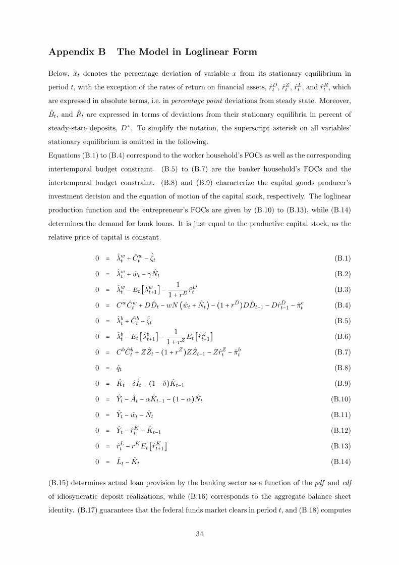
Appendix B The Model in Loglinear Form

Below, xt denotes the percentage deviation of variable x from its stationary equilibrium in

period t, with the exception of the rates of return on financial assets, rDt , rZ

t , rLt , and rR

t , which

are expressed in absolute terms, i.e. in percentage point deviations from steady state. Moreover,

Bt, and Rt are expressed in terms of deviations from their stationary equilibria in percent of

steady-state deposits, D∗. To simplify the notation, the superscript asterisk on all variables’

stationary equilibrium is omitted in the following.

Equations (B.1) to (B.4) correspond to the worker household’s FOCs as well as the corresponding

intertemporal budget constraint. (B.5) to (B.7) are the banker household’s FOCs and the

intertemporal budget constraint. (B.8) and (B.9) characterize the capital goods producer’s

investment decision and the equation of motion of the capital stock, respectively. The loglinear

production function and the entrepreneur’s FOCs are given by (B.10) to (B.13), while (B.14)

determines the demand for bank loans. It is just equal to the productive capital stock, as the

relative price of capital is constant.

0 = λwt + Cw

t − ζt (B.1)

0 = λwt + wt − γNt (B.2)

0 = λwt −Et [λw

t+1] − 1

1 + rDrDt (B.3)

0 = CwCwt +DDt −wN (wt + Nt) − (1 + rD)DDt−1 −DrD

t−1 − πet (B.4)

0 = λbt + Cb

t − ζt (B.5)

0 = λbt −Et [λb

t+1] − 1

1 + rZEt [rZ

t+1] (B.6)

0 = CbCbt +ZZt − (1 + rZ)ZZt−1 −ZrZ

t − πbt (B.7)

0 = qt (B.8)

0 = Kt − δIt − (1 − δ)Kt−1 (B.9)

0 = Yt − At − αKt−1 − (1 − α)Nt (B.10)

0 = Yt − wt − Nt (B.11)

0 = Yt − rKt − Kt−1 (B.12)

0 = rLt − rKEt [rK

t+1] (B.13)

0 = Lt − Kt (B.14)

(B.15) determines actual loan provision by the banking sector as a function of the pdf and cdf

of idiosyncratic deposit realizations, while (B.16) corresponds to the aggregate balance sheet

identity. (B.17) guarantees that the federal funds market clears in period t, and (B.18) computes

34

the aggregate level of interbank borrowing (≡ interbank lending). (B.19) and (B.20) are the

loglinearized profit functions of goods-producing firms and banks, respectively, while (B.21)

reflects the free-entry condition into financial intermediation. Recall that free entry implies

that both expected individual and realized aggregate profits in the banking sector are driven

down to zero.

0 = LLt − κZZt + (1 − ξ) {F ((κ − 1)Z) [(κ − 1)ZZt −DDt] + σ2f((κ − 1)Z)σt}−{[(κ − 1)Z −D]F ((κ − 1)Z) + σ2f((κ − 1)Z)} ξt (B.15)

0 = DRt +LLt −DDt −ZZt (B.16)

0 = (κ − 1)ZZt −DDt (B.17)

0 = DBt − {[(κ − 1)Z −D]F ((κ − 1)Z) + σ2f((κ − 1)Z)} ξt

−ξ {F ((κ − 1)Z) [(κ − 1)ZZt −DDt] + σ2f((κ − 1)Z)} σt (B.18)

0 = πet − Y Yt − q(1 − δ)K (qt + Kt−1) +wN (wt + Nt)+(1 + r)qK (qt−1 + Kt−1) + qKrL

t−1 (B.19)

0 = Etπbt+1 − (rL − rR)LLt −L(rL

t − rRt ) + (rD − rR)DDt +D(rD

t − rRt )

+(rZ − rR)ZZt +Z(EtrZt+1 − rR

t ) (B.20)

0 = πbt (B.21)

With unconventional monetary policy, equations (B.15), (B.16), (B.18), and (B.20) are adjusted

accordingly. Moreover, (B.22) is the loglinear version of the feedback rule used for broad liquidity

injections.29

0 = X − φ (rLt − rD

t ) (B.22)

29Recall that excess reserves Rt, interbank borrowing Bt, and central bank liquidity injections Xt are expressedin terms of percent deviations from steady-state deposits D.

35

Appendix C Probability Density Functions

6 7 8 9 10 11 12 13 140

0.05

0.1

0.15

0.2

0.25

0.3

0.35

0.4

Lt=κZ

t

dt(i)+Z

t

f(d

t(i)+

Zt)

(a) Complete access to the federal funds market

6 7 8 9 10 11 12 13 140

0.05

0.1

0.15

0.2

0.25

0.3

0.35

0.4

Lt

κZt

dt(i)+Z

t

f(d

t(i)+

Zt)

(b) Incomplete access to the federal funds market

Figure C.1: Effect of interbank borrowing & lending on aggregate bank loans to entrepreneurs

6 7 8 9 10 11 12 13 140

0.05

0.1

0.15

0.2

0.25

0.3

0.35

0.4

dt(i)+Z

t

f(d

t(i)+

Zt)

Lt

κZt

(a) Uncertainty shock (σt = 1→ 1.1) for ξt = .5

6 7 8 9 10 11 12 13 140

0.05

0.1

0.15

0.2

0.25

0.3

0.35

0.4

Lt

κZt

dt(i)+Z

t

f(d

t(i)+

Zt)

(b) Financial friction shock (ξt = .5→ .4) for σt = 1

Figure C.2: Effect of shocks to financial intermediation on aggregate volume of federal funds

6 7 8 9 10 11 12 13 140

0.05

0.1

0.15

0.2

0.25

0.3

0.35

0.4

Lt

κZt

dt(i)+Z

t+X

t

f(d

t(i)+

Zt+

Xt)

(a) Uncertainty shock (σt = 1→ 1.1) for ξt = .5

6 7 8 9 10 11 12 13 140

0.05

0.1

0.15

0.2

0.25

0.3

0.35

0.4

Lt

κZt

dt(i)+Z

t+X

t

f(d

t(i)+

Zt+

Xt)

(b) Financial friction shock (ξt = .5→ .4) for σt = 1

Figure C.3: Effect of broad central bank liquidity injections in response to financial shocks

36

References

Afonso, G., Lagos, R., 2012. An Empirical Study of Trade Dynamics in the Fed Funds Market.

Federal Reserve Bank of New York Staff Report 550.

Ashcraft, A., McAndrews, J., Skeie, D., 2011. Precautionary reserves and the interbank market.

Journal of Money, Credit, and Banking, Supplement to 43, 311–348.

Bech, M. L., Klee, E., 2011. The mechanics of graceful exit: Interest on reserves and segmenta-

tion in the federal funds market. Journal of Monetary Economics 58 (5), 415–431.

Bernanke, B. S., Gertler, M., 1989. Agency Costs, Net Worth, and Business Fluctuations.

American Economic Review 79 (1), 14–31.

Bernanke, B. S., Gertler, M., Gilchrist, S., 1999. The Financial Accelerator in a Quantitative

Business Cycle Framework. In: Taylor, J. B., Woodford, M. (Eds.), Handbook of Macroeco-

nomics. Elsevier, Amsterdam: North-Holland, pp. 1341–1393.

Bhattacharya, S., Fulghieri, P., 1994. Uncertain liquidity and interbank contracting. Economics

Letters 44 (3), 287–294.

Bloom, N., 2009. The impact of uncertainty shocks. Econometrica 77 (3), 623–685.

Brunnermeier, M. K., 2009. Deciphering the Liquidity and Credit Crunch 2007-2008. Journal

of Economic Perspectives 23 (1), 77–100.

Calvo, G. A., 1983. Staggered prices in a utility-maximizing framework. Journal of Monetary

Economics 12 (3), 383–398.

Carlstrom, C. T., Fuerst, T. S., 1997. Agency Costs, Net Worth, and Business Fluctuations: A

Computable General Equilibrium Analysis. American Economic Review 87 (5), 893–910.

Carpenter, S., Demiralp, S., Eisenschmidt, J., 2013. The Effectiveness of the Non-Standard

Policy Measures during the Financial Crises: The Experiences of the Federal Reserve and the

European Central Bank. ECB Working Paper Series 1562.

Chari, V. V., Christiano, L. J., Eichenbaum, M., 1995. Inside Money, Outside Money, and

Short-Term Interest Rates. Journal of Money, Credit and Banking 27 (4), 1354–1386.

Christensen, I., Dib, A., 2008. The financial accelerator in an estimated New Keynesian model.

Review of Economic Dynamics 11 (1), 155–178.

Christiano, L. J., Motto, R., Rostagno, M., 2010. Financial Factors in Economic Fluctuations.

ECB Working Paper Series 1192.

Cook, D., 1999. The liquidity effect and money demand. Journal of Monetary Economics 43 (2),

377–390.

Dib, A., 2010. Banks, Credit Market Frictions, and Business Cycles. Bank of Canada Working

Paper 2010-24.

37

Ennis, H. M., Keister, T., 2008. Understanding Monetary Policy Implementation. Federal Re-

serve Bank of Richmond Economic Quarterly 94 (3), 235–263.

Ennis, H. M., Weinberg, J. A., 2013. Over-the-counter loans, adverse selection, and stigma in

the interbank market. Forthcoming in: Review of Economic Dynamics.

Ennis, H. M., Wolman, A. L., 2012. Large Excess Reserves in the U.S.: A View from the

Cross-Section of Banks. Federal Reserve Bank of Richmond Working Paper No. 12-05.

Fernandez-Villaverde, J., Guerron-Quintana, P. A., Rubio-Ramırez, J., Uribe, M., 2011. Risk

matters: the real effects of volatility shocks. American Economic Review 101 (6), 2530–2561.

Freixas, X., Parigi, B. M., Rochet, J.-C., 2000. Systemic Risk, Interbank Relations, and Liquid-

ity Provision by the Central Bank. Journal of Money, Credit, and Banking 32 (3), 611–638.

Frost, P. A., 1971. Banks’ Demand for Excess Reserves. Journal of Political Economy 79 (4),

805–825.

Furfine, C. H., 2001. The reluctance to borrow from the Fed. Economics Letters 72 (2), 209–213.

Gerali, A., Neri, S., Sessa, L., Signoretti, F. M., 2010. Credit and Banking in a DSGE Model

of the Euro Area. Journal of Money, Credit and Banking, Supplement to 42, 107–141.

Gertler, M., Karadi, P., 2011. A model of unconventional monetary policy. Journal of Monetary

Economics 58 (1), 17–34.

Gertler, M., Kiyotaki, N., 2011. Financial Intermediation and Credit Policy in Business Cycle

Analysis. In: Friedman, B. M., Woodford, M. (Eds.), Handbook of Monetary Economics.

Elsevier, Amsterdam: North-Holland, pp. 547–599.

Hellwig, M. F., 1994. Liquidity provision, banking, and the allocation of interest rate risk.

European Economic Review 38 (7), 1363–1389.

Holmstrom, B., Tirole, J., 1998. Private and Public Supply of Liquidity. Journal of Political

Economy 106 (1), 1–40.

Kaufman, H. M., Lombra, R. E., 1980. The Demand for Excess Reserves, Liability Management,

and the Money Supply Process. Economic Inquiry 18 (4), 555–566.

Keister, T., McAndrews, J., 2009. Why are banks holding so many excess reserves? Federal

Reserve Bank of New York Staff Report 380.

Kiyotaki, N., Moore, J., 2008. Liquidity, Business Cycles, and Monetary Policy. Society for

Economic Dynamics 2008 Meeting Papers 35.

McAndrews, J., Sarkar, A., Wang, Z., 2008. The Effect of the Term Auction Facility on the

London Inter-Bank Offered Rate. Federal Reserve Bank of New York Staff Report 335.

Peristiani, S., 1998. The Growing Reluctance to Borrow at the Discount Window: An Empirical

Investigation. The Review of Economics and Statistics 80 (4), 611–620.

38

Poole, W., 1968. Commercial Bank Reserve Management in a Stochastic Model: Implications

for Monetary Policy. Journal of Finance 23 (5), 769–791.

Rochet, J.-C., Tirole, J., 1996. Interbank Lending and Systemic Risk. Journal of Money, Credit

and Banking 28 (4), 733–762.

Saunders, A., Urich, T., 1988. The Effects of Shifts in Monetary Policy and Reserve Accounting

Regimes on Bank Reserve Management Behavior in the Federal Funds Market. Journal of

Banking and Finance 12 (4), 523–535.

Taylor, J. B., Williams, J. C., 2009. A Black Swan in the Money Market. American Economic

Journal: Macroeconomics 1 (1), 58–83.

von Thadden, E.-L., 1997. The term-structure of investment and the banks’ insurance function.

European Economic Review 41 (7), 1355–1374.

Wen, Y., 2011. Input and Output Inventory Dynamics. American Economic Journal: Macroe-

conomics 3 (4), 181–212.

Williamson, S. D., 1987. Financial Intermediation, Business Failures, and Real Business Cycles.

Journal of Political Economy 95 (6), 1196–1216.

Woodford, M., 2010. Financial Intermediation and Macroeconomic Analysis. Journal of Eco-

nomic Perspectives 24 (4), 21–44.

Wu, T., 2008. On the effectiveness of the Federal Reserve’s new liquidity facilities. Federal

Reserve Bank of Dallas Working Paper Series 0808.

Wu, T., 2011. The U.S. Money Market and the Term Auction Facility in the Financial Crisis

of 2007-2009. The Review of Economics and Statistics 93 (2), 617–631.

39

Tables

Table 1: Calibration of parameters for the stationary and dynamic simulation of quarterly data

Benchmark Parameter Values

α βw βb γ δ κ N∗ rR∗ ξ∗ σ∗

1/3 .995 .94 1 .025 12.5 1/3 0 1 1

Table 2: Steady-state values corresponding to the benchmark parameter calibration in Table 1

Steady-State Values

K∗/4Y ∗ Cw∗/Y ∗ Cb∗/Y ∗ I∗/Y ∗ Z∗/L∗ Z∗/D∗ B∗/D∗ R∗/D∗2.400 .7110 .0490 .2400 .0800 .0870 .0437 0

D∗/4Y ∗ L∗/4Y ∗ rD∗ rL∗ rK∗ rZ∗ πe∗ πb∗

2.208 2.400 .0050 .0097 .0347 .0638 0 0

Table 3: Calibration of parameters for unconventional monetary policy interventions

Monetary Policy Parameter Values

φ rX∗ rR∗

800 .00125 0

40

Figures

1980 1985 1990 1995 2000 2005 20100

5

10

15

20

% o

f deposits

Bankruptcy of

Lehman Brothers

Total reserves minus required reserves (all depository institutions, weekly data)

1980 1985 1990 1995 2000 2005 2010

2

4

6

8

% o

f deposits

Federal Funds and Reverse RP with banks (all commercial banks, weekly data)

Figure 1: Excess reserves and federal funds transactions of banks in the U.S. as a fraction of totaldeposits; weekly data from January 1975 to December 2011

41

0 20 40−0.2

−0.1

0

0.1

0.2Output Y

0 20 40−20

−15

−10

−5

0

Investment I

0 20 40−0.1

−0.05

0Worker Consumption C

w

0 20 400

0.005

0.01

0.015

0.02Banker Consumption C

b

0 20 40−0.1

−0.05

0

0.05

0.1Employment N

0 20 40

−0.1

−0.05

0Real Wage w

0 20 400

0.005

0.01

0.015

0.02Household Deposits D

0 20 40−0.5

−0.4

−0.3

−0.2

−0.1

Bank Loans L

0 20 400

0.1

0.2

0.3

0.4

Federal Funds B

0 20 400

0.1

0.2

0.3

0.4

Bank Reserves R

0 20 400

1

2

3

4

5x 10

−3 Spread rL − r

D

0 20 400

5

10

Uncertainty Shock σ

ξ*= 1

ξ*= .5

ξ*=0

Figure 2: Selected impulse responses to a shock in the variance of deposit realizations

Vertical axes: Deviations from steady state in % (percentage points for rL and rD; as a fraction of steady-statedeposits for B and R); Horizontal axes: Quarters after the exogenous shock

0 20 40−0.2

−0.1

0

0.1

0.2Output Y

0 20 40−20

−15

−10

−5

0

Investment I

0 20 40−0.1

−0.05

0Worker Consumption C

w

0 20 400

0.005

0.01

0.015

0.02Banker Consumption C

b

0 20 40−0.1

−0.05

0

0.05

0.1Employment N

0 20 40

−0.1

−0.05

0Real Wage w

0 20 400

0.005

0.01

0.015

0.02Household Deposits D

0 20 40−0.5

−0.4

−0.3

−0.2

−0.1

Bank Loans L

0 20 40−0.5

−0.4

−0.3

−0.2

−0.1

Federal Funds B

0 20 400

0.1

0.2

0.3

0.4

Bank Reserves R

0 20 400

1

2

3

4

5x 10

−3 Spread rL − r

D

0 20 40−10

−5

0

Financial Friction Shock ξ

ξ*= 1

ξ*= .5

Figure 3: Selected impulse responses to an increase in the federal funds market friction

Vertical axes: Deviations from steady state in % (percentage points for rL and rD; as a fraction of steady-statedeposits for B and R); Horizontal axes: Quarters after the exogenous shock

42

2007 2007.5 2008 2008.5 2009 2009.5 2010 2010.5 2011 2011.5 2012−15

−10

−5

0

5

10

15

20

25

% o

f deposits

Sources of reserve balances (weekly data)

Announcement

of TAF creation

Bankruptcy of

Lehman Brothers

Total reserve balances with FRBs

Reserves added through Fed lending facilities

Reserves added through asset purchase programs

Figure 4: Sources of reserve balances in the U.S. as a fraction of total deposits; weekly data fromJanuary 2007 to December 2012 (compare Ennis and Wolman, 2012, Figure 2)

Notes: Reserves added through Fed’s lending facilities sum “term auction credit”, “central bank liquidity swaps”,and “loans”, while Reserves added through asset purchases equal “total factors supplying reserve balances” less“total factors, other than reserve balances, absorbing reserve funds” and reserves added through lending facilities.All time series are downloaded from the H.4.1 Statistical Release of the Board of Governors of the Federal Reserveand expressed as a fraction of total deposits.

0 20 40−0.01

−0.005

0Output Y

0 20 40−1

−0.5

0Investment I

ξ*= .9

ξ*= .5

ξ*= .1

0 20 40−0.01

−0.005

0

0.005

0.01Worker Consumption C

w

0 20 40−20

−15

−10

−5

0

x 10−3Banker Consumption C

b

0 20 40−5

0

5x 10

−3 Employment N

0 20 40−0.02

−0.015

−0.01

−0.005

0Household Deposits D

0 20 40−0.02

−0.015

−0.01

−0.005

0Bank Loans L

0 20 400

0.5

1

1.5

2x 10

−3 Spread rL − r

D

0 20 400

0.5

1Federal Funds B

0 20 400

0.5

1Bank Reserves R

0 20 400

0.5

1C.b. injection X

0 20 400

5

10

Uncertainty Shock σ

Figure 5: Selected impulse responses to an uncertainty shock with targeted liquidity injection

Vertical axes: Deviations from steady state in % (percentage points for rL and rD; as a fraction of steady-statedeposits for B and R); Horizontal axes: Quarters after the exogenous shock

43

0 20 40−0.01

−0.005

0Output Y

0 20 40−1

−0.5

0Investment I

0 20 40−0.01

−0.005

0

0.005

0.01Worker Consumption C

w

0 20 40−20

−15

−10

−5

0

x 10−3Banker Consumption C

b

0 20 40−5

0

5x 10

−3 Employment N

0 20 40−0.02

−0.015

−0.01

−0.005

0Household Deposits D

0 20 40−0.02

−0.015

−0.01

−0.005

0Bank Loans L

0 20 400

0.5

1

1.5

2x 10

−3 Spread rL − r

D

0 20 400

0.5

1Federal Funds B

0 20 400

0.5

1Bank Reserves R

0 20 400

0.5

1C.b. injection X

0 20 400

5

10

Uncertainty Shock σ

ξ*= .9

ξ*= .5

ξ*= .1

Figure 6: Selected impulse responses to an uncertainty shock with broad liquidity injection

Vertical axes: Deviations from steady state in % (percentage points for rL and rD; as a fraction of steady-statedeposits for B and R); Horizontal axes: Quarters after the exogenous shock

0 20 40−0.1

−0.05

0Output Y

0 20 40−10

−5

0Investment I

ξ*= .9

ξ*= .5

ξ*= .1

0 20 40−0.1

−0.05

0

0.05

0.1Worker Consumption C

w

0 20 40−0.2

−0.15

−0.1

−0.05

0

Banker Consumption Cb

0 20 40−0.05

0

0.05Employment N

0 20 40−0.2

−0.15

−0.1

−0.05

0Household Deposits D

0 20 40−0.2

−0.15

−0.1

−0.05

0Bank Loans L

0 20 400

0.005

0.01Spread r

L − r

D

0 20 40−4

−3

−2

−1

0Federal Funds B

0 20 400

5

10Bank Reserves R

0 20 400

5

10C.b. injection X

0 20 40−10

−5

0

Financial Friction Shock ξ

Figure 7: Selected impulse responses to a financial friction shock with targeted liquidity injection

Vertical axes: Deviations from steady state in % (percentage points for rL and rD; as a fraction of steady-statedeposits for B and R); Horizontal axes: Quarters after the exogenous shock

44

0 20 40−0.1

−0.05

0Output Y

0 20 40−10

−5

0Investment I

0 20 40−0.1

−0.05

0

0.05

0.1Worker Consumption C

w

0 20 40−0.2

−0.15

−0.1

−0.05

0

Banker Consumption Cb

0 20 40−0.05

0

0.05Employment N

0 20 40−0.2

−0.15

−0.1

−0.05

0Household Deposits D

0 20 40−0.2

−0.15

−0.1

−0.05

0Bank Loans L

0 20 400

0.005

0.01Spread r

L − r

D

0 20 40−4

−3

−2

−1

0Federal Funds B

0 20 400

5

10Bank Reserves R

0 20 400

5

10C.b. injection X

0 20 40−10

−5

0

Financial Friction Shock ξ

ξ*= .9

ξ*= .5

ξ*= .1

Figure 8: Selected impulse responses to a financial friction shock with broad liquidity injection

Vertical axes: Deviations from steady state in % (percentage points for rL and rD; as a fraction of steady-statedeposits for B and R); Horizontal axes: Quarters after the exogenous shock

45