Embed Size (px)
Citation preview
THE EZNSS CFD CODETHEORETICAL AND USER’S MANUAL
Revision 330
ISCFDC Report 2015-06
Prepared by
Yuval Levy and Daniella Raveh
ISCFDC LTD
COPYRIGHT c⃝ October 2015
by
The authors and the Israeli CFD Center
i
Contents
Abstract . . . . . . . . . . . . . . . . . . . . . . . . . . . . . . . . . . . . . x
1 Introduction 1
2 Computational Methods 3
2.1 Introduction . . . . . . . . . . . . . . . . . . . . . . . . . . . . . . . . 3
2.2 Governing Equations . . . . . . . . . . . . . . . . . . . . . . . . . . . 3
2.2.1 Normalizing the Continuity Equation . . . . . . . . . . . . . . 5
2.2.2 Normalizing the Momentum Equation . . . . . . . . . . . . . 7
2.2.2.1 Turbulent Viscosity Coefficient . . . . . . . . . . . . 8
2.2.3 Normalizing the Energy Equation . . . . . . . . . . . . . . . . 9
2.2.3.1 Turbulent Heat Conduction Coefficient . . . . . . . . 10
2.2.4 Equation of State . . . . . . . . . . . . . . . . . . . . . . . . . 11
2.2.5 Constitutive Relations . . . . . . . . . . . . . . . . . . . . . . 12
2.2.6 Real Gas Effects . . . . . . . . . . . . . . . . . . . . . . . . . 13
2.2.7 Normalized Set of Equation . . . . . . . . . . . . . . . . . . . 14
2.3 General Curvilinear Coordinates . . . . . . . . . . . . . . . . . . . . . 14
2.4 Implicit Numerical Methods . . . . . . . . . . . . . . . . . . . . . . . 18
2.5 Beam and Warming Algorithm . . . . . . . . . . . . . . . . . . . . . 19
2.6 Flux Vector Splitting . . . . . . . . . . . . . . . . . . . . . . . . . . . 21
2.6.1 Steger Warming Flux Splitting . . . . . . . . . . . . . . . . . 23
2.6.2 F3D Algorithm . . . . . . . . . . . . . . . . . . . . . . . . . . 23
2.7 Flux Difference Splitting . . . . . . . . . . . . . . . . . . . . . . . . . 24
2.7.1 HLLC . . . . . . . . . . . . . . . . . . . . . . . . . . . . . . . 25
Israeli Computational Fluid Dynamics Center LTD
ii
2.7.2 AUSM . . . . . . . . . . . . . . . . . . . . . . . . . . . . . . . 27
2.7.3 MAPS . . . . . . . . . . . . . . . . . . . . . . . . . . . . . . . 29
2.8 Dual Time Step Formulation . . . . . . . . . . . . . . . . . . . . . . . 31
2.9 Turbulence Models . . . . . . . . . . . . . . . . . . . . . . . . . . . . 33
2.9.1 Baldwin-Lomax Turbulence Model . . . . . . . . . . . . . . . 34
2.9.2 Degani-Schiff Modification . . . . . . . . . . . . . . . . . . . . 36
2.9.3 Goldberg One-Equation Model . . . . . . . . . . . . . . . . . 37
2.9.4 Spalart-Allmaras Turbulence Model . . . . . . . . . . . . . . . 40
2.9.5 Unified Hybrid RANS/LES k − ω-TNT Turbulence Model . . 41
2.9.6 Reynolds Stress Models . . . . . . . . . . . . . . . . . . . . . . 44
3 Computational Mesh Topology 45
3.1 Introduction . . . . . . . . . . . . . . . . . . . . . . . . . . . . . . . . 45
3.2 Chimera . . . . . . . . . . . . . . . . . . . . . . . . . . . . . . . . . . 46
3.2.1 Hole Cutting . . . . . . . . . . . . . . . . . . . . . . . . . . . 46
3.2.1.1 Multi Zone Bodies . . . . . . . . . . . . . . . . . . . 46
3.2.1.2 Variable Thickness and Selective Hole Cutting . . . . 47
3.2.2 Virtual Body Hole Cutting . . . . . . . . . . . . . . . . . . . . 47
3.2.3 Fail Safe Mechanism for Interpolations Searches . . . . . . . . 48
3.3 Patched Grids . . . . . . . . . . . . . . . . . . . . . . . . . . . . . . . 49
3.4 Single Mesh Topology . . . . . . . . . . . . . . . . . . . . . . . . . . 49
3.4.1 Examples . . . . . . . . . . . . . . . . . . . . . . . . . . . . . 50
3.4.2 Grid Generation . . . . . . . . . . . . . . . . . . . . . . . . . . 54
3.5 Elliptic Collar Grids . . . . . . . . . . . . . . . . . . . . . . . . . . . 54
3.5.1 Introduction . . . . . . . . . . . . . . . . . . . . . . . . . . . . 54
3.5.2 Fuselage Surface . . . . . . . . . . . . . . . . . . . . . . . . . 55
3.5.3 Intersection Between a Line and a Discrete Surface . . . . . . 56
3.5.4 Wing Surface . . . . . . . . . . . . . . . . . . . . . . . . . . . 57
3.5.5 Volume Boundaries . . . . . . . . . . . . . . . . . . . . . . . . 57
3.5.6 Grid Generation . . . . . . . . . . . . . . . . . . . . . . . . . . 57
3.5.7 Force and Moment Calculations . . . . . . . . . . . . . . . . . 58
Israeli Computational Fluid Dynamics Center LTD
iii
3.6 Hyperbolic Collar Grids . . . . . . . . . . . . . . . . . . . . . . . . . 58
4 Boundary Conditions 60
4.1 Introduction . . . . . . . . . . . . . . . . . . . . . . . . . . . . . . . . 60
4.2 Wall Boundary Conditions . . . . . . . . . . . . . . . . . . . . . . . . 60
4.3 Inflow, Outflow, and Extrapolations . . . . . . . . . . . . . . . . . . . 61
4.3.1 Characteristic-like Inflow Outflow . . . . . . . . . . . . . . . . 61
4.4 Periodic Boundary Conditions . . . . . . . . . . . . . . . . . . . . . . 62
4.5 Cut Conditions in I Direction . . . . . . . . . . . . . . . . . . . . . . 62
4.6 Axis Conditions . . . . . . . . . . . . . . . . . . . . . . . . . . . . . . 62
4.7 Symmetry Conditions . . . . . . . . . . . . . . . . . . . . . . . . . . . 62
4.8 Free Stream Conditions . . . . . . . . . . . . . . . . . . . . . . . . . . 63
4.9 Inlet Conditions . . . . . . . . . . . . . . . . . . . . . . . . . . . . . . 63
4.10 Zonal Boundary Conditions . . . . . . . . . . . . . . . . . . . . . . . 63
5 Six Degrees of Freedom Simulation 64
5.1 Translational Equation of Motion . . . . . . . . . . . . . . . . . . . . 64
5.2 Rotational Equation of Motion . . . . . . . . . . . . . . . . . . . . . 65
5.2.1 Quaternions . . . . . . . . . . . . . . . . . . . . . . . . . . . . 67
5.3 Store Location Update . . . . . . . . . . . . . . . . . . . . . . . . . . 67
6 Static and Dynamic Aeroelasticity 69
6.1 Static Aeroelasticity . . . . . . . . . . . . . . . . . . . . . . . . . . . 70
6.2 Equations of Motion for Uncoupled Aeroelastic Motion . . . . . . . . 71
6.2.1 Numerical Scheme . . . . . . . . . . . . . . . . . . . . . . . . 71
6.2.2 Solution Method . . . . . . . . . . . . . . . . . . . . . . . . . 72
6.3 Mesh Deformations using the TFI Approach . . . . . . . . . . . . . . 72
6.3.1 Face Deformations . . . . . . . . . . . . . . . . . . . . . . . . 73
6.3.2 Volume Deformations . . . . . . . . . . . . . . . . . . . . . . . 75
7 Parallelization 77
7.1 Introduction . . . . . . . . . . . . . . . . . . . . . . . . . . . . . . . . 77
Israeli Computational Fluid Dynamics Center LTD
iv
7.2 Single-Level Parallelism . . . . . . . . . . . . . . . . . . . . . . . . . 78
7.3 Multi-Level Parallelism . . . . . . . . . . . . . . . . . . . . . . . . . . 80
8 Summary 83
A Jacobian Matrices 84
A.1 Inviscid Flux Vectors Jacobian Matrices . . . . . . . . . . . . . . . . 84
A.2 Jacobian Matrix of the Viscous Flux Vector . . . . . . . . . . . . . . 85
B Jacobian Matrices Eigensystems 87
B.1 Eigenvectors . . . . . . . . . . . . . . . . . . . . . . . . . . . . . . . . 87
B.2 Eigenvalues . . . . . . . . . . . . . . . . . . . . . . . . . . . . . . . . 88
C Input Files 89
C.1 Input File Names and Types . . . . . . . . . . . . . . . . . . . . . . . 89
C.2 Main Input File eznss.i.defaults . . . . . . . . . . . . . . . . . . . . . 89
C.3 Array Input File eznssa.i . . . . . . . . . . . . . . . . . . . . . . . . . 107
C.4 Collar Grid Generation Input File cgg.i . . . . . . . . . . . . . . . . . 124
C.5 Six Degrees of Freedom Motion Simulation Input File 6dof.i . . . . . 126
C.6 Virtual Body File Inputs eznssvb.i . . . . . . . . . . . . . . . . . . . 133
C.7 Elliptic Collar Grid Update File Inputs ecgu.i . . . . . . . . . . . . . 136
C.8 Spline Inputs in File spline.i . . . . . . . . . . . . . . . . . . . . . . . 137
C.9 Flap Inputs in File flap.i . . . . . . . . . . . . . . . . . . . . . . . . . 141
C.10 Rotor Inputs in File rotor.i . . . . . . . . . . . . . . . . . . . . . . . 143
D Data Files 145
D.1 Rationale . . . . . . . . . . . . . . . . . . . . . . . . . . . . . . . . . 145
D.2 Input Data Files . . . . . . . . . . . . . . . . . . . . . . . . . . . . . 145
D.3 Output Data Files . . . . . . . . . . . . . . . . . . . . . . . . . . . . 146
D.4 Files with Specific Designation . . . . . . . . . . . . . . . . . . . . . . 147
D.5 Aeroelasticity Input Output Files . . . . . . . . . . . . . . . . . . . . 147
D.5.1 Input Files . . . . . . . . . . . . . . . . . . . . . . . . . . . . . 147
D.5.2 Output Files . . . . . . . . . . . . . . . . . . . . . . . . . . . . 149
Israeli Computational Fluid Dynamics Center LTD
v
D.6 Six Degrees of Freedom Motion Simulation Input Files . . . . . . . . 151
D.7 Non-Standard Atmosphere Input File . . . . . . . . . . . . . . . . . . 154
D.8 Specific Heat Polynomial Coefficients Input File . . . . . . . . . . . . 155
D.9 Inlet Mass Flow Rate Control Input File . . . . . . . . . . . . . . . . 155
D.10 Jet Input Files . . . . . . . . . . . . . . . . . . . . . . . . . . . . . . 156
D.11 Discrete Force Input Files . . . . . . . . . . . . . . . . . . . . . . . . 157
D.12 Sectional Force and Moment Output . . . . . . . . . . . . . . . . . . 158
E Test Cases 159
E.1 Flow Solver . . . . . . . . . . . . . . . . . . . . . . . . . . . . . . . . 159
E.1.1 RAE 2822 Super Critical Airfoil . . . . . . . . . . . . . . . . . 159
E.1.2 NACA 4412 Airfoil . . . . . . . . . . . . . . . . . . . . . . . . 164
E.1.3 Onera M6 Transonic Wing . . . . . . . . . . . . . . . . . . . . 169
E.2 Aeroelasticity Module . . . . . . . . . . . . . . . . . . . . . . . . . . 172
E.2.1 Basic Wing-Fuselage-Tail Test-Case - The PHDP . . . . . . . 172
E.2.2 Multi-block Wing . . . . . . . . . . . . . . . . . . . . . . . . . 176
E.2.3 Constrained Deformations - Wing-tip Missile . . . . . . . . . . 179
E.2.4 Flaps . . . . . . . . . . . . . . . . . . . . . . . . . . . . . . . . 180
E.2.5 Prescribed Sinusoidal Flap Motion . . . . . . . . . . . . . . . 183
Bibliography 191
Israeli Computational Fluid Dynamics Center LTD
vi
List of Figures
2.1 Wave structure of the HLLC Riemann solver . . . . . . . . . . . . . . 26
3.1 Chimera computational mesh (with virtual body hole cutting) about
a multi-element airfoil . . . . . . . . . . . . . . . . . . . . . . . . . . 48
3.2 C-O grid topology . . . . . . . . . . . . . . . . . . . . . . . . . . . . . 51
3.3 C-H grid topology . . . . . . . . . . . . . . . . . . . . . . . . . . . . . 51
3.4 C-C grid topology . . . . . . . . . . . . . . . . . . . . . . . . . . . . . 52
3.5 C-O grid topology for wings . . . . . . . . . . . . . . . . . . . . . . . 53
3.6 Two zone grid topology for wings . . . . . . . . . . . . . . . . . . . . 53
3.7 C grid topology . . . . . . . . . . . . . . . . . . . . . . . . . . . . . . 55
3.8 C type hyperbolic collar grid . . . . . . . . . . . . . . . . . . . . . . . 59
6.1 Computational space . . . . . . . . . . . . . . . . . . . . . . . . . . . 74
D.1 Polynomial input file format (polyforce.in) . . . . . . . . . . . . . . . 152
D.2 Force file input file format (forcefile 101.in) . . . . . . . . . . . . . . 153
D.3 Fractional input file format (fracforce.in) . . . . . . . . . . . . . . . . 154
D.4 An example of a typical input file (density.dat) . . . . . . . . . . . . 157
D.5 Discrete force input file format (discreteforcefile [100 + force number].in)157
D.6 File format for (surface force list.dat) . . . . . . . . . . . . . . . . . . 158
E.1 RAE 2822 computational mesh . . . . . . . . . . . . . . . . . . . . . 160
E.2 Pressure coefficient . . . . . . . . . . . . . . . . . . . . . . . . . . . . 160
E.3 Flow conditions for the RAE 2822 case 9 . . . . . . . . . . . . . . . . 161
E.4 Time step, method, and restart info for the RAE 2822 case 9 . . . . . 162
Israeli Computational Fluid Dynamics Center LTD
vii
E.5 Turbulence model input (k − ω-TNT) for the RAE 2822 case 9 . . . . 163
E.6 Turbulence model input (RSM-MCL) for the RAE 2822 case 9 . . . . 163
E.7 NACA 4412 computational mesh . . . . . . . . . . . . . . . . . . . . 164
E.8 Stream-wise velocity at the stationx
C= 0.953 . . . . . . . . . . . . . 165
E.9 Convergence time history . . . . . . . . . . . . . . . . . . . . . . . . . 166
E.10 Flow conditions for the NACA 4412 case . . . . . . . . . . . . . . . . 166
E.11 Time step and spatial accuracy for the NACA 4412 case . . . . . . . 167
E.12 Method for the NACA 4412 case (HLLC) . . . . . . . . . . . . . . . . 167
E.13 Method for the NACA 4412 case (Steger-Warming . . . . . . . . . . . 167
E.14 Restart info for the NACA 4412 case . . . . . . . . . . . . . . . . . . 168
E.15 Turbulence model input for the NACA 4412 case . . . . . . . . . . . 168
E.16 Onera M6 computational mesh, color coded surface pressure, and tur-
bulent viscosity contour lines . . . . . . . . . . . . . . . . . . . . . . . 169
E.17 Time step and method for the Onera M6 case . . . . . . . . . . . . . 170
E.18 Turbulence model input (k − ω-TNT) for the Onera M6 case . . . . . 170
E.19 Pressure coefficient aty
b/2= 0.9 . . . . . . . . . . . . . . . . . . . . . 171
E.20 Sample grid file grid s 101.dat . . . . . . . . . . . . . . . . . . . . . . 173
E.21 Sample modes file mode s 101.dat . . . . . . . . . . . . . . . . . . . . 174
E.22 Elastic related inputs in the main input file eznss.i.defaults . . . . . . 174
E.23 Spline related inputs in the main input file eznss.i.defaults . . . . . . 175
E.24 First entries in input file spline.i . . . . . . . . . . . . . . . . . . . . . 175
E.25 Structural grid of the PHDP wing . . . . . . . . . . . . . . . . . . . . 176
E.26 First elastic mode shape mapped to the surface grid . . . . . . . . . . 177
E.27 Aerodynamic surface grid of the MB wing . . . . . . . . . . . . . . . 177
E.28 Structural grid of the MB wing . . . . . . . . . . . . . . . . . . . . . 178
E.29 First entries in input file spline.i . . . . . . . . . . . . . . . . . . . . . 178
E.30 First elastic mode shape mapped to the MB surface grids . . . . . . . 179
E.31 Wing-tip Missile Test-case - Before and After Elastic Deformatiom . . 180
E.32 Defining the wing-tip missile sub-domain - main input file . . . . . . 180
E.33 Defining the wing-tip missile sub-domain - array input file . . . . . . 181
E.34 Defining the attachment point in input file spline.i . . . . . . . . . . 181
Israeli Computational Fluid Dynamics Center LTD
viii
E.35 Defining the number of flaps in the main input file . . . . . . . . . . . 181
E.36 Flap input file . . . . . . . . . . . . . . . . . . . . . . . . . . . . . . . 182
E.37 Surface mesh of PHDP wing with deflected trailing-edge flap . . . . . 183
E.38 Defining elastic and flap inputs in the main input file for the case of
flap prescribed sinusoidal motion . . . . . . . . . . . . . . . . . . . . 185
E.39 Flap input file for the case of flap prescribed sinusoidal motion . . . . 186
Israeli Computational Fluid Dynamics Center LTD

ix
List of Tables
2.1 List of dimensionless variables . . . . . . . . . . . . . . . . . . . . . . 6
2.2 Turbulence length scales . . . . . . . . . . . . . . . . . . . . . . . . . 44
Israeli Computational Fluid Dynamics Center LTD
x
Abstract
This theoretical manual describes the algorithms, methods, and input and output
files of the EZNSS code. The current revision of the code, revision 262, contains a
flow solver, a Chimera suite, an elliptic collar grid generator, a six degrees of freedom
motion simulation module, an aeroelasticity module, and a spline suite to support the
aeroelasticity module. The flow solver contains a central differencing method (Beam
and Warming), a flux vector splitting method (Steger-Warming), a partially flux
vector splitting method (F3D), and three flux difference splitting methods (HLLC,
AUSM+up, and MAPS). It has explicit and implicit time marching, with our without
dual-time-stepping, and with or without Runge-Kutta (3rd and 5th order). The flow
solver has 6 RANS turbulence models, the algebraic Baldwin-Lomax, its Degani-Schiff
variant, the Rt by Goldberg, the Spalart-Allmaras turbulence model, the k−ω-TNT,and the k − ω-SST. The k − ω-TNT model contains flags that turns it into various
types of a hybrid model, named the XLES, the DDES, and the X−DDES models.
The solver also has three Reynolds Stress models, the JH model, the stress omega
model, and the MCL model (although included in the production version of the
code, Reynolds stress models are not fully tested yet, use with care). The Chimera
suite contains virtual body hole cutting and fail safe mechanisms for interpolations.
The aeroelasticity module is based on the Karpel-Raveh modal approach, and the
spline suite is due to Dr. Daniella Raveh. The code is fully parallel, using multi-level
parallelism for the flow solver.
Israeli Computational Fluid Dynamics Center LTD
1
Chapter 1
Introduction
The EZNSS code is a multi-zone Euler/Navier-Stokes flow solver. The EZNSS code
is capable of simulating complex, time-accurate flows about dynamically deforming
geometries. This includes relative motion between surfaces as well as deformations
caused due to aeroelastic effects. The code contains a number of implicit algorithms
and a number of turbulence models. The code handles complex geometries using
patched grids or the Chimera overset grid topology [1]. The code automatically
handles various grid topologies such as C-C, C-H, and C-O grid topologies. When the
grid topology is identified, the appropriate boundary conditions are set. To provide
higher flexibility, the user may override the boundary conditions using the input file.
The code is written using Fortran 77 and Fortran 90. The use of Fortran 90 allows
to use dynamic memory allocation. The program is parallelized using OpenMP and
multi-level parallelism and may be run on any shared memory parallel computer
with relative ease. Version 2.5.2 of the code contains the dual-time step capability,
aeroelastic capabilities, six degrees of freedom motion simulation, and real gas effects.
The report is arranged in the following manner: Chapter 2 contains a description
of the governing equations, numerical algorithms, and the turbulence models that are
used in the code. Chapter 3 describes the supported mesh topologies, with examples.
Chapter 4 contains a brief description of the boundary conditions. Chapter 5 entails
the six degrees of freedom simulation module while Chapter 6 entails the aeroelasticity
module. Parallelization is described in Chapter 7.
Israeli Computational Fluid Dynamics Center LTD

Introduction 2
The appendices provide additional information as follows: Appendices A and B
include details of the Jacobians. Appendices C and D include detailed descriptions
of the input and data files, along with some usage guidance.
Israeli Computational Fluid Dynamics Center LTD
3
Chapter 2
Computational Methods
2.1 Introduction
Computer simulations are generally based upon the numerical solution of the model
equations in a discretized mode. The accuracy of the computations depends mainly
on the physical modeling, the numerical algorithm, and the quality of the computa-
tional mesh. This chapter contains a description of the governing equations for high
Reynolds number fluid flow, the numerical algorithms that are used in the solution
of the Euler or the Navier-Stokes equations, the boundary conditions associated with
them, and turbulence models that are used to model the Reynolds stress tensor. The
Reynolds stress tensor may be modeled by adopting the Boussinesq approximation
or by using Reynolds stress models.
2.2 Governing Equations
The equations governing fluid flow are derived from the laws of conservation of mass,
momentum, and energy. The set of five partial differential equations is known as the
Navier-Stokes equations and can be represented in a conservation-law form that is
convenient for numerical simulations, namely
∂Q
∂t+∂ (E − Ev)
∂x+∂ (F − Fv)
∂y+∂ (G−Gv)
∂z= 0 (2.1)
Israeli Computational Fluid Dynamics Center LTD
Computational Methods 4
where Q is the vector of conserved mass, momentum, and energy
Q =
ρ
ρu
ρv
ρw
e
(2.2)
The inviscid flux vectors, E, F , and G, are
E =
ρu
ρu2 + p
ρuv
ρuw
u (e+ p)
, F =
ρv
ρuv
ρv2 + p
ρvw
v (e+ p)
, G =
ρw
ρuw
ρvw
ρw2 + p
w (e+ p)
(2.3)
and the viscous flux vectors, Ev, Fv, and Gv, are
Ev =
0
τxx
τyx
τzx
βx
, Fv =
0
τxy
τyy
τzy
βy
, Gv =
0
τxz
τyz
τzz
βz
(2.4)
Israeli Computational Fluid Dynamics Center LTD
Computational Methods 5
whereτxx = λ
(∂u∂x
+ ∂v∂y
+ ∂w∂z
)+ 2µ∂u
∂x
τyy = λ(
∂u∂x
+ ∂v∂y
+ ∂w∂z
)+ 2µ∂v
∂y
τzz = λ(
∂u∂x
+ ∂v∂y
+ ∂w∂z
)+ 2µ∂w
∂z
τxy = τyx = µ(
∂u∂y
+ ∂v∂x
)τxz = τzx = µ
(∂u∂z
+ ∂w∂x
)τyz = τzy = µ
(∂v∂z
+ ∂w∂y
)βx = uτxx + vτxy + wτxz + κ∂T
∂x
βy = uτyx + vτyy + wτyz + κ∂T∂y
βz = uτzx + vτzy + wτzz + κ∂T∂z
(2.5)
where T is the temperature. Stokes hypothesis, λ = −23µ, is typically used to further
simplify Equation (2.5).
For computational purposes these equations are made dimensionless. [2] Charac-
teristic values of all the variables can be formed from six basic reference quantities: a
reference length, L, e.g. the chord of a wing or the diameter of a body of revolution;
a reference velocity, a∞, the speed of sound of the undisturbed flow; reference density
and temperature, characteristic of the undisturbed flow, ρ∞ and T∞, respectively;
and similarly, reference values for the coefficients of viscosity and thermal conduc-
tivity, µ∞ and κ∞, characteristic of the undisturbed flow. In addition, for real gas
effects, there is a need to define a reference value for specific heat capacity in constant
pressure cp, cp∞ .
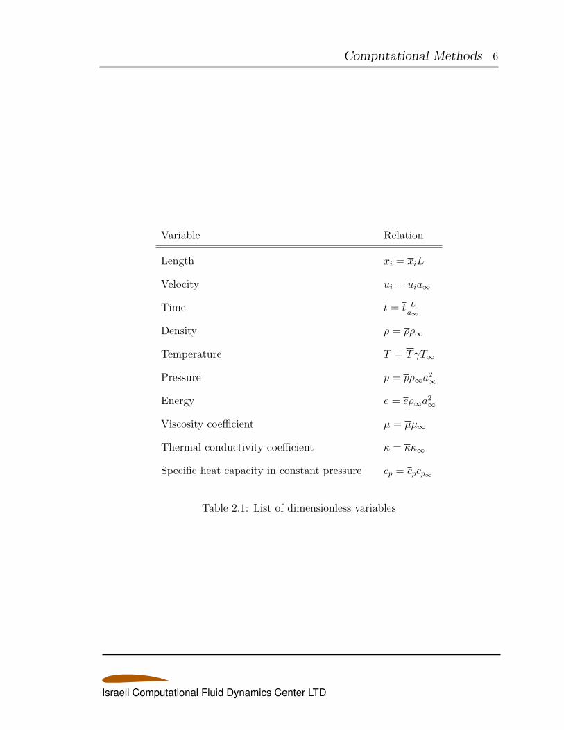
The other reference values are derived from the basic ones. Thus time t is nor-
malized by L/a∞ and the pressure p and the energy e are normalized by ρa2∞. The
temperature T is normalized by the reference value γ∞T∞. Table 2.1 contains a list
of normalization relations. These relations assist in normalizing the equations.
2.2.1 Normalizing the Continuity Equation
The continuity equation in Cartesian coordinates is given by:
∂ρ
∂t+∂ρu
∂x+∂ρv
∂y+∂ρw
∂z= 0 (2.6)
Israeli Computational Fluid Dynamics Center LTD
Computational Methods 6
Variable Relation
Length xi = xiL
Velocity ui = uia∞
Time t = t La∞
Density ρ = ρρ∞
Temperature T = TγT∞
Pressure p = pρ∞a2∞
Energy e = eρ∞a2∞
Viscosity coefficient µ = µµ∞
Thermal conductivity coefficient κ = κκ∞
Specific heat capacity in constant pressure cp = cpcp∞
Table 2.1: List of dimensionless variables
Israeli Computational Fluid Dynamics Center LTD
Computational Methods 7
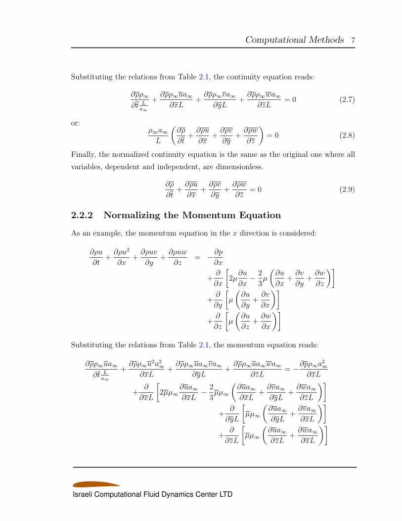
Substituting the relations from Table 2.1, the continuity equation reads:
∂ρρ∞
∂t La∞
+∂ρρ∞ua∞∂xL
+∂ρρ∞va∞∂yL
+∂ρρ∞wa∞
∂zL= 0 (2.7)
or:ρ∞a∞L
(∂ρ
∂t+∂ρu
∂x+∂ρv
∂y+∂ρw
∂z
)= 0 (2.8)
Finally, the normalized continuity equation is the same as the original one where all
variables, dependent and independent, are dimensionless.
∂ρ
∂t+∂ρu
∂x+∂ρv
∂y+∂ρw
∂z= 0 (2.9)
2.2.2 Normalizing the Momentum Equation
As an example, the momentum equation in the x direction is considered:
∂ρu
∂t+∂ρu2
∂x+∂ρuv
∂y+∂ρuw
∂z= −∂p
∂x
+∂
∂x
[2µ∂u
∂x− 2
3µ
(∂u
∂x+∂v
∂y+∂w
∂z
)]+∂
∂y
[µ
(∂u
∂y+∂v
∂x
)]+∂
∂z
[µ
(∂u
∂z+∂w
∂x
)]Substituting the relations from Table 2.1, the momentum equation reads:
∂ρρ∞ua∞
∂t La∞
+∂ρρ∞u
2a2∞∂xL
+∂ρρ∞ua∞va∞
∂yL+∂ρρ∞ua∞wa∞
∂zL= −∂pρ∞a
2∞
∂xL
+∂
∂xL
[2µµ∞
∂ua∞∂xL
− 2
3µµ∞
(∂ua∞∂xL
+∂va∞∂yL
+∂wa∞∂zL
)]+
∂
∂yL
[µµ∞
(∂ua∞∂yL
+∂va∞∂xL
)]+
∂
∂zL
[µµ∞
(∂ua∞∂zL
+∂wa∞∂xL
)]
Israeli Computational Fluid Dynamics Center LTD
Computational Methods 8
Multiplying both sides of the equation withL
ρ∞a2∞results in:
∂ρu
∂t+∂ρu2
∂x+∂ρuv
∂y+∂ρuw
∂z= −∂p
∂x+
µ∞
ρ∞a∞L×
∂
∂x
[2µ∂u
∂x− 2
3µ
(∂u
∂x+∂v
∂y+∂w
∂z
)]+∂
∂y
[µ
(∂u
∂y+∂v
∂x
)]+∂
∂z
[µ
(∂u
∂z+∂w
∂x
)]
Realizing that the termµ∞
ρ∞a∞Lequals
M
Rewhere Re =
ρ∞u∞L
µ∞results in:
∂ρu
∂t+∂ρu2
∂x+∂ρuv
∂y+∂ρuw
∂z= −∂p
∂x+M
Re×
∂
∂x
[2µ∂u
∂x− 2
3µ
(∂u
∂x+∂v
∂y+∂w
∂z
)]+∂
∂y
[µ
(∂u
∂y+∂v
∂x
)]+∂
∂z
[µ
(∂u
∂z+∂w
∂x
)]2.2.2.1 Turbulent Viscosity Coefficient
In turbulent flows the viscosity coefficient is composed of the molecular viscosity
coefficient, µl, and the turbulent viscosity coefficient, µt such that:
µ = µl + µt (2.10)
with the dimensionless viscosity coefficient being:
µ = µl + µt (2.11)
The molecular viscosity coefficient is evaluated using Sutherland’s Law while the
turbulent viscosity coefficient is obtained through the solution of the turbulence model
Israeli Computational Fluid Dynamics Center LTD
Computational Methods 9
equations.
2.2.3 Normalizing the Energy Equation
In Cartesian coordinates, the energy equation reads:
∂e
∂t+∂ (eu+ p)
∂x+∂ (ev + p)
∂y+∂ (ew + p)
∂z=
∂
∂x
(uτxx + vτxy + wτxz + κ
∂T
∂x
)∂
∂y
(uτyx + vτyy + wτyz + κ
∂T
∂y
)∂
∂z
(uτzx + vτzy + wτzz + κ
∂T
∂z
)(2.12)
Based on the normalization conducted for the momentum equation, the shear stresses’
dimensionless form is:
τij =µ∞a∞L
τ ij (2.13)
Substituting the relations from Table 2.1, the energy equation reads:
∂eρ∞a2∞
∂t La∞
+∂ (eρ∞a
2∞ua∞ + pρ∞a
2∞)
∂xL+
∂ (eρ∞a2∞va∞ + pρ∞a
2∞)
∂yL+∂ (eρ∞a
2∞wa∞ + pρ∞a
2∞)
∂zL=
∂
∂xL
(ua∞
µ∞a∞L
τxx + va∞µ∞a∞L
τxy + wa∞µ∞a∞L
τxz + κκ∞∂TγT∞∂xL
)∂
∂yL
(ua∞
µ∞a∞L
τ yx + va∞µ∞a∞L
τ yy + wa∞µ∞a∞L
τ yz + κκ∞∂TγT∞∂yL
)∂
∂zL
(ua∞
µ∞a∞L
τ zx + va∞µ∞a∞L
τ zy + wa∞µ∞a∞L
τ zz + κκ∞∂TγT∞∂zL
)(2.14)
Israeli Computational Fluid Dynamics Center LTD
Computational Methods 10
Multiplying both sides of the equation withL
ρ∞a3∞results in:
∂e
∂t+∂ (eu+ p)
∂x+∂ (ev + p)
∂y+∂ (ew + p)
∂z=
µ∞
ρ∞a∞L×[
∂
∂x
(uτxx + vτxy + wτxz +
κ∞γT∞a2∞µ∞
κ∂T
∂x
)∂
∂y
(uτ yx + vτ yy + wτ yz +
κ∞γT∞a2∞µ∞
κ∂T
∂y
)∂
∂z
(uτ zx + vτ zy + wτ zz +
κ∞γT∞a2∞µ∞
κ∂T
∂z
)](2.15)
As with the momentum equation, the termµ∞
ρ∞a∞L=
M
Re. Realizing that a2∞ =
γRT∞, the termκ∞γT∞a2∞µ∞
becomesκ∞Rµ∞
. The dimensionless energy equation then
becomes:
∂e
∂t+∂ (eu+ p)
∂x+∂ (ev + p)
∂y+∂ (ew + p)
∂z=M
Re×[
∂
∂x
(uτxx + vτxy + wτxz +
κ∞Rµ∞
κ∂T
∂x
)∂
∂y
(uτ yx + vτ yy + wτ yz +
κ∞Rµ∞
κ∂T
∂y
)∂
∂z
(uτ zx + vτ zy + wτ zz +
κ∞Rµ∞
κ∂T
∂z
)](2.16)
2.2.3.1 Turbulent Heat Conduction Coefficient
In turbulent flows the heat conduction coefficient is composed of the thermal heat
conduction coefficient, κl, and the turbulent heat conduction coefficient, κt such that:
κ = κl + κt (2.17)
with the dimensionless conductivity coefficient being:
κ = κl + κt (2.18)
Israeli Computational Fluid Dynamics Center LTD
Computational Methods 11
The thermal heat conduction coefficient is evaluated using a relation that is similar
to the Sutherland Law while the turbulent heat conduction coefficient is evaluated
based on the turbulent viscosity coefficient, µt and the turbulent Prandtl number:
Prt =µtcpκt
(2.19)
The turbulent Prandtl number itself may be assumed constant (Prt ≈ 0.9) or it can be
evaluated using empirical relations. Hence, the turbulent heat conduction coefficient
may be evaluated using:
κt =µtcpPrt
(2.20)
When using dimensionless form, one has to evaluate κt as follows:
Prt =µtµ∞cpcp∞κtκ∞
=µ∞cp∞κ∞
µtcpκt
(2.21)
or:
Prt = Pr∞µtcpκt
(2.22)
and therefore:
κt = Pr∞µtcpPrt
(2.23)
2.2.4 Equation of State
To close the system of fluid dynamics equations it is necessary to establish relations
between the thermodynamics variables, p, ρ, T , and eI . For most problems in gas
dynamics, it is possible to assume a perfect gas. This assumption is also adopted in
the EZNSS code. Hence, in Equations (2.3) and (2.5), the pressure and temperature
are obtained from the equation of state for a perfect gas
p = ρRT = ρ (γ − 1) eI (2.24)
where R is the gas constant (R = 287.0 for air), eI is the internal energy of the gas,
and γ is the ratio of specific heats (cp/cv). In terms of the flow variables, the pressure
Israeli Computational Fluid Dynamics Center LTD
Computational Methods 12
and temperature are calculated using:
p = (γ − 1)
[e− 1
2ρ(u2 + v2 + w2
)]T =
γ − 1
R
[e
ρ− 1
2
(u2 + v2 + w2
)](2.25)
Following the normalization process that is described in the previous sections, the
equation of state is normalized as follows:
pρ∞a2∞ = ρρ∞RTγT∞ (2.26)
Once again, realizing that a2∞ = γRT∞, the normalized equation of state becomes:
p = ρT (2.27)
and the normalized pressure and temperature are evaluated using:
p = (γ − 1)
[e− 1
2ρ(u2 + v2 + w2
)]T =
p
ρ(2.28)
2.2.5 Constitutive Relations
In addition to the equation of state, it is also necessary to establish relations for the
coefficients of viscosity, µ, and thermal conductivity, κ. The EZNSS code utilizes the
Sutherland Formulae to evaluate the coefficients as follows:
µ = 1.458× 10⁻⁶ T32
T + 110.4
κ = 2.495× 10⁻³ T32
T + 194(2.29)
Israeli Computational Fluid Dynamics Center LTD
Computational Methods 13
Using the normalization definitions from Table 2.1, the normalized Sutherland For-
mulae become:
µ =
(1 +
110.4
T∞
) (γT) 3
2
γT + 110.4T∞
κ =
(1 +
194
T∞
) (γT) 3
2
γT + 194T∞
(2.30)
2.2.6 Real Gas Effects
For high speed flows, air no longer behaves as a calorically perfect gas. The simplest
model is to account for the changes in specific heats by using polynomial relations.
The following model uses two polynomials, one for temperatures bellow T = 1000K
and one for temperatures above T = 1000K. Both polynomials take the form:
cpR
= a0 + a1T + a2T2 + a3T
3 + a4T4 (2.31)
The default polynomial coefficients are given by:
a0 = 3.56839620E + 00
a1 = −6.78729429E − 04
a2 = 1.55371476E − 06
a3 = −3.29937060E − 12
a4 = −4.66395387E − 13 (2.32)
for temperatures bellow T = 1000K and
a0 = 3.08792717E + 00
a1 = 1.24597184E − 03
a2 = −4.23718945E − 07
a3 = 6.74774789E − 11
a4 = −3.97076972E − 15 (2.33)
Israeli Computational Fluid Dynamics Center LTD
Computational Methods 14
for temperatures above T = 1000K. Once cp is calculated, the ratio of specific heats
may be evaluated using:
γ =cp
cp −R(2.34)
The default polynomial coefficients may be changed using a user input file as described
in Appendix D.8.
2.2.7 Normalized Set of Equation
The normalization process results in a set of dimensionless equations that is similar
to the dimensional ones with two exceptions. The factor M/Re appears in front of
the viscous terms, where Re is the Reynolds number
Re =ρ∞u∞L
µ∞(2.35)
Also, the term κ in Eq. (2.5) becomes κ∞Rµ∞
κ. The rest of the variables appear in the
same way with the addition of a bar and the set of normalized equations takes the
form∂Q
∂t+∂E
∂x+∂F
∂y+∂G
∂z=M
Re
(∂Ev
∂x+∂F v
∂y+∂Gv
∂z
)(2.36)
Note: From here on the bars above all variables are omitted and a normalized physical
domain with normalized flow variables is assumed.
2.3 General Curvilinear Coordinates
The Cartesian form of the equations is not suitable for handling complex body geome-
tries. For example, application of the boundary conditions are not compatible with
the Cartesian form. To enhance compatibility the physical domain is transformed
into a computational one by introducing a coordinate transformation.[2–4] In general
Israeli Computational Fluid Dynamics Center LTD
Computational Methods 15
terms, this transformation takes the form
τ = t
ξ = ξ (x, y, z, t)
η = η (x, y, z, t)
ζ = ζ (x, y, z, t)
(2.37)
The transformation brings the body surface f (x, y, z) = 0 onto one computational
plane (in the current formulation ζ = 1). Therefore the coordinate ζ extends radially
from the body surface and the other two coordinates, ξ and η lie on the surface normal
to ζ. The computational domain is equi-spaced (usually chosen to be δξ = δη = δζ =
1, for convenience), so the differencing is simplified. To apply the transformation to
the model equations the chain rule is used∂∂t∂∂x∂∂y
∂∂z
=
1 ξt ηt ζt
0 ξx ηx ζx
0 ξy ηy ζy
0 ξz ηz ζz
∂∂τ∂∂ξ
∂∂η
∂∂ζ
(2.38)
The Jacobian of the transformation J is given by the determinant
J−1 = ∂(t,x,y,z)∂(τ,ξ,η,ζ)
=
∣∣∣∣∣∣∣∣∣∣1 xτ yτ zτ
0 xξ yξ zξ
0 xη yη zη
0 xζ yζ zζ
∣∣∣∣∣∣∣∣∣∣J−1 = xξ (yηzζ − yζzη)− yξ (xηzζ − xζzη) + zξ (xηyζ − xζyη) (2.39)
Israeli Computational Fluid Dynamics Center LTD
Computational Methods 16
The metrics of the transformation are given by
ξt = −xτξx − yτξy − zτξz
ξx = J (yηzζ − zηyζ)
ξy = −J (xηzζ − xζzη)
ξz = J (xηyζ − xζyη)
ηt = −xτηx − yτηy − zτηz
ηx = −J (yξzζ − yζzξ)
ηy = J (xξzζ − xζzξ)
ηz = −J (xηyζ − xζyη)
ζt = −xτζx − yτζy − zτζz
ζx = J (yξzη − yηzξ)
ζy = −J (xξzη − xηzξ)
ζz = J (xξyη − xηyξ)
(2.40)
Applying the coordinate transformation results in a new set of equations that main-
tains the conservation-law form of the original equations. Equation (2.36) becomes
∂Q
∂τ+∂E
∂ξ+∂F
∂η+∂G
∂ζ=
1
Re
(∂Ev
∂ξ+∂Fv
∂η+∂Gv
∂ζ
)(2.41)
whereQ = 1
JQ
E = 1J
(Qξt + Eξx + Fξy +Gξz)
F = 1J
(Qηt + Eηx + Fηy +Gηz)
G = 1J
(Qζt + Eζx + Fζy +Gζz)
Ev = 1J
(Evξx + Fvξy +Gvξz)
Fv = 1J
(Evηx + Fvηy +Gvηz)
Gv = 1J
(Evζx + Fvζy +Gvζz)
(2.42)
Alternatively, the new dependent variables, the inviscid flux vectors, and the viscous
flux vectors can be expressed in terms of the original dependent variables and metrics
Israeli Computational Fluid Dynamics Center LTD
Computational Methods 17
as
Q =1
J
ρ
ρu
ρv
ρw
e
E =
1
J
ρU
ρuU + ξxp
ρvU + ξyp
ρwU + ξzp
(e+ p)U − ξtp
F =1
J
ρV
ρuV + ηxp
ρvV + ηyp
ρwV + ηzp
(e+ p)V − ηtp
G =
1
J
ρW
ρuW + ζxp
ρvW + ζyp
ρwW + ζzp
(e+ p)W − ζtp
(2.43)
Ev =1
ReJ
0
ξxτxx + ξyτxy + ξzτxz
ξxτyx + ξyτyy + ξzτyz
ξxτzx + ξyτzy + ξzτzz
ξxβx + ξyβy + ξzβz
Fv =1
ReJ
0
ηxτxx + ηyτxy + ηzτxz
ηxτyx + ηyτyy + ηzτyz
ηxτzx + ηyτzy + ηzτzz
ηxβx + ηyβy + ηzβz
Gv =1
ReJ
0
ζxτxx + ζyτxy + ζzτxz
ζxτyx + ζyτyy + ζzτyz
ζxτzx + ζyτzy + ζzτzz
ζxβx + ζyβy + ζzβz
(2.44)
Israeli Computational Fluid Dynamics Center LTD

Computational Methods 18
where U , V , and W are the contravariant velocities and are given by the relationU − ξt
V − ηt
W − ζt
=
ξx ξy ξz
ηx ηy ηz
ζx ζy ζz
u
v
w
(2.45)
Each element containing derivatives with respect to the original independent variables
t, x, y, z has to be expanded according to the chain rule so that the final form of
the equations includes only derivatives with respect to the transformed independent
variables τ , ξ, η, and ζ.
2.4 Implicit Numerical Methods
The fine grid spacing required to resolve the normal viscous terms close to the body
surface rules out the use of explicit methods. In explicit time-marching schemes
the maximum time step is proportional to the minimum grid spacing. As a result
the time-step limit imposed by stability is very small. In contrast, even though the
operation count per time step is high, it is more efficient to use implicit methods. The
development of a non-iterative implicit algorithm for the solution of the Navier-Stokes
equations requires a time linearization of the nonlinear vectors. The linearization
procedure is simple since the equations are written in conservation-law form. It is
done by utilizing local Taylor series expansions of the vectors E, F , and G about
Q [5, 6]
En+1 = En + An(Qn+1 − Qn
)+O
(∆t2)
F n+1 = F n + Bn(Qn+1 − Qn
)+O
(∆t2)
Gn+1 = Gn + Cn(Qn+1 − Qn
)+O
(∆t2) (2.46)
where A, B, and C are the Jacobian matrices. The superscript n denotes evaluation
at the nth time step where t = n∆t. The elements of A, B, and C, are given in
Appendix A.
A similar Taylor series expansion of the viscous flux vectors results in the viscous
Israeli Computational Fluid Dynamics Center LTD
Computational Methods 19
Jacobian matrices, Av, Bv, and Cv. However, the viscous Jacobians contain mixed
derivatives and therefore the block tridiagonal form of the linear systems is spoiled.
In first order, the mixed derivatives can be neglected with no loss of accuracy and
simpler matrices, that are in fact based on the thin-layer approximation [7] can be
used. The new matrices, denoted by Aξv, B
ηv , and C
ζv , contain derivatives only in the
direction denoted by the superscript. The elements of Aξv, B
ηv , and C
ζv are also given
in Appendix A.
Applying the first-order Euler implicit formula to Eq.(2.36) and incorporating the
linearizations results in a linear system with first-order time accuracyI + h
[∂
∂ξA+
∂
∂ηB +
∂
∂ζC − 1
Re
(∂
∂ξAξ
v +∂
∂ηBη
v +∂
∂ζCζ
v
)]n
∆Qn =
−∆t
[∂E
∂ξ+∂F
∂η+∂G
∂ζ− 1
Re
(∂Ev
∂ξ+∂Fv
∂η+∂Gv
∂ζ+
)]n+O
(∆t2)
(2.47)
where I is the identity matrix, h = ∆t, ∆Qn = Qn+1 − Qn, and ∂/∂ξ, ∂/∂η, and
∂/∂ζ are approximated by finite differencing.
2.5 Beam and Warming Algorithm
The linear system, formed after replacing the spatial derivatives in Eq. (2.47) with
central finite difference approximations, is a block hepta-diagonal matrix with nonad-
jacent diagonals. A direct solution of this system requires inversion of a block matrix
of the size of the computational mesh. Because of the large band of the system, the
direct inversion process is a very costly one and calls for a simplification. Approxi-
mate factorization of the left-hand-side operator reduces the inversion to a sequence
of one-dimensional inversions, without altering the formal accuracy of Eq. (2.47) [5].
If central differencing is used to approximate the spatial operators, the resulting
one-dimensional operators are block tridiagonal matrices. Beam and Warming [5]
developed a factored algorithm applicable to the Euler gasdynamic equations in two
dimensions. They later included the viscous flux terms and applied the scheme to the
two-dimensional compressible Navier-Stokes equations [6]. The following form of the
Israeli Computational Fluid Dynamics Center LTD
Computational Methods 20
algorithm is its extension to three dimensions.(I + hδξA− hRe−1δξA
ξv
)n (I + hδηB − hRe−1δηB
ηv
)n(I + hδζC − hRe−1δζC
ζv
)n∆Qn = Rn (2.48)
where Rn is
Rn = −∆t[δξE + δηF + δζG−Re−1
(δξEv + δηFv + δζGv
)]n(2.49)
The above formulation applies to both Euler implicit first-order and trapezoidal
second-order time accuracy as follows: setting the quantity h equal to ∆t yields
the first-order-accurate Euler implicit form, while setting h equal to ∆t/2 yields the
second-order-accurate trapezoidal form. The δ operators denote central differencing
and the δ operators denote a midpoint operator used in order to preserve the block
tridiagonal form. The numerical scheme then has second-order spatial accuracy and
either first- or second-order time accuracy.
The procedure of advancing the solution from time-step n to time-step n + 1
requires a series of three one-dimensional block-tridiagonal inversions(I + hδξA− hRe−1δξA
ξv
)n∆Q1 = Rn(
I + hδηB − hRe−1δηBηv
)n∆Q2 = ∆Q1(
I + hδζC − hRe−1δζCζv
)n∆Qn = ∆Q2
Qn+1 = Qn +∆Qn (2.50)
Each inversion process is set up in a way that takes advantage of the pipelining capa-
bility of supercomputers. Although the inversion is in itself recursive, the factorized
scheme can be optimized by performing concurrent multiple line inversions, further
reducing the computation time per time step.
Israeli Computational Fluid Dynamics Center LTD
Computational Methods 21
2.6 Flux Vector Splitting
Finite difference schemes that are based on centered spatial difference operators are
simultaneously stable for both the positive and the negative characteristic speeds as-
sociated with the convective flux vectors. The Beam andWarming algorithm is a good
example. It is constructed from Eq. (2.47) by using central differences to approximate
all of the spatial derivatives. Although the scheme is unstable in three dimensions,
the instability is a weak one and can be controlled by numerical dissipation that is
added to damp the growth of high-frequency waves and nonlinear instabilities. On
the other hand, one-sided difference operators lead to schemes that are stable only
for equations with single-signed eigenvalues. However, these schemes have better
dissipative and dispersive properties. One-sided difference operators also lead to a
lower-banded matrix than the block-tridiagonal matrix that is usually formed with
central differencing, and therefore lead to an easier inversion. The gasdynamic equa-
tions have characteristic speeds (eigenvalues) of mixed signs in subsonic flow regimes;
therefore the use of one-sided spatial-difference operators (upwind schemes) requires
splitting the flux terms.
Upwinding requires that the flux vector, (for example E in Eq. (2.47), and its
Jacobian matrix (in this case A) be split into sub-vectors and sub-matrices associated
with its positive and negative eigenvalues. This can be done by realizing that the
Jacobian matrices A, B, and C have a complete set of eigenvalues and eigenvectors
and therefore can be written as
A = TξΛξT−1ξ , B = TηΛηT
−1η , C = TζΛζT
−1ζ (2.51)
The eigenvalues Λξ, Λη, and Λζ and the eigenvectors Tξ, Tη, and Tζ are given in
Appendix B.
Using the result of Eq. (2.51) and the fact that E is a homogeneous function of
degree one in Q, Steger and Warming [8] rewrote E as
E = TξΛξT−1ξ Q (2.52)
Israeli Computational Fluid Dynamics Center LTD
Computational Methods 22
where the diagonal elements of the matrix Λξ are given by Eq. (B.2). Any eigenvalue
λl, l = 1 . . . 5 can be rewritten as
λl = λ+l + λ−l (2.53)
where
λ+l =λl + |λl|
2, λ−l =
λl − |λl|2
(2.54)
Using this formula one can rewrite the diagonal matrix Λξ
Λξ = Λ+ξ + Λ−
ξ (2.55)
where Λ+ξ has the diagonal elements λ+l and Λ−
ξ has the diagonal elements λ−l . Thus
Eq. (2.52) can be rewritten as
E = Tξ
(Λ+
ξ + Λ−ξ
)T−1ξ Q
E =(A+ + A−
)Q
E =(E+ + E−
)(2.56)
with
A = A+ + A−, A+ = TξΛ+ξ T
−1ξ , A− = TξΛ
−ξ T
−1ξ
E+ = A+Q, E− = A−Q
Israeli Computational Fluid Dynamics Center LTD
Computational Methods 23
2.6.1 Steger Warming Flux Splitting
Using the flux vector splitting as described above, the following three-factored algo-
rithm has been devised by Steger and Warming. [8](I + hδbξA
+ + hδfξ A− − hRe−1δξA
ξv
)n(I + hδbηB
+ + hδfη B− − hRe−1δηB
ηv
)n(2.57)(
I + hδbζC+ + hδfζ C
− − hRe−1δζCζv
)n∆Qn = Rn (2.58)
where
Rn = −∆t[δbξE
+ + δfξ E− + δbηF
+ + δfη F− + δbζG
+ + δfζ G− −Re−1
(δξEv + δηFv + δζGv
)]n(2.59)
Here h = ∆t or ∆t/2 for first- or second-order time accuracy, δb is a backward-
difference operator and δf is a forward-difference operator. This scheme is also ap-
proximately factored, based on the same principles that led to the Beam and Warming
algorithm, in order to obtain a block-tridiagonal linear system. The procedure for
advancing the solution using the Steger Warming algorithm is similar to the proce-
dure used in the Beam and Warming algorithm. Both algorithms have three factors,
one for each coordinate direction. This provides the means to devise a method that
combines the two types of differencing is different directions. The EZNSS code con-
tains the capability to choose either central or upwind differencing in each coordinate
separately.
2.6.2 F3D Algorithm
Steger et al [9] proposed another alternative to using central differencing or flux vector
splitting in all directions. By splitting and upwind-differencing the convective flux
vector in the streamwise direction, while maintaining a central difference operator for
Israeli Computational Fluid Dynamics Center LTD
Computational Methods 24
the crossflow fluxes, a two-factored, partially flux-split algorithm is formed[I + hδbξA
+ + hδζC − hRe−1δζCζv
]n[I + hδfξ A
− + hδηB − hRe−1δζBηv
]n∆Qn = Rn (2.60)
where
Rn = −∆t[δbξE
+ + δfξ E− + δηF + δζG−Re−1
(δξEv + δηFv + δζGv
)]n(2.61)
This scheme is also approximately factored in order to obtain a block-tridiagonal
linear system. The procedure for advancing the solution using the two-factor method
is as follows: [I + hδbξA
+ + hδζC − hRe−1δζCζv
]n∆Q1 = Rn[
I + hδfξ A− + hδηB − hRe−1δζB
ηv
]n∆Qn = ∆Q1
Qn+1 = Qn +∆Qn (2.62)
Due to the upwinding, the first step is solved by a forward sweep, from ξ = ξmin to
ξ = ξmax, followed by a backward sweep, from ξ = ξmax to ξ = ξmin for the second
step.
The two-factored algorithm has better stability properties and was found to be
unconditionally stable when applied to a linear model wave equation [10]. It also has
better dissipative and dispersive properties due to the flux splitting in the streamwise
direction. Numerical dissipation terms are still needed in the crossflow directions,
however, since central-difference operators are used there to approximate the spatial
derivatives.
2.7 Flux Difference Splitting
An exact solution of the Riemann problem is computationally expensive and therefore
approximate Riemann solvers are commonly used. Flux difference splitting utilizes
Israeli Computational Fluid Dynamics Center LTD
Computational Methods 25
the solution of the approximate Riemann problem to evaluate the fluxes at cell faces.
In what follows, the three FDS methods that are used in EZNSS are described in
detail.
2.7.1 HLLC
The concept of average-state approximations was introduced by Harten, Lax and van-
Leer [11] in 1983. The Harten, Lax and van-Leer (HLL) scheme is attractive because
of its robustness, conceptual simplicity, and ease of coding, but it has the serious
flaw of a diffusive contact surface. This is mainly because the HLL solver reduces
the exact Riemann problem to two pressure waves and therefore neglects the contact
surface. Toro et al [12] discussed this limitation, and proposed a modified three wave
solver, named HLLC, where the contact is explicitly present. This HLLC schemes is
found to have the following properties: 1) exact preservation of isolated contact and
shear waves, 2) positivity preserving of scalar quantity, and 3) enforcement of the
entropy condition. The resulting scheme greatly improves contact resolution and has
been successfully used to compute compressible viscous and turbulent flows [13].
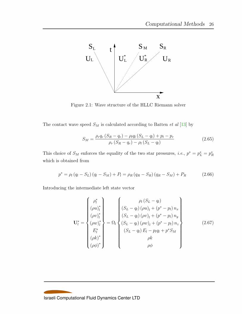
The HLLC Riemann solver as proposed by Batten et al [13] is implemented in
the EZNSS code. The HLLC scheme assumes two intermediate states, U∗L and U∗
R
within the region bounded by the left moving wave, SL, and the right moving wave,
SR (the subscripts L and R denote the left and right states of the Riemann solver,
respectively). The states U∗L and U∗
R are split by the contact wave, which moves with
the velocity SM (see Figure 2.1).
The wave speeds SL and SR are computed according to Einfeldt et al [14] as
follows:
SL =Min[λl, λRoel ] (2.63)
SR =Max[λm, λRoem ] (2.64)
where λl is the smallest eigenvalue and λm is the largest eigenvalue. Similarly, λRoel and
λRoem are the smallest and largest eigenvalues of the Roe matrix [15], respectively. The
normal velocity to the interface is denoted by q and is defined as q = unx+vny+wnz.
Israeli Computational Fluid Dynamics Center LTD
Computational Methods 26
x
M
UR* UR
tUL
*UL
LS S SR
Figure 2.1: Wave structure of the HLLC Riemann solver
The contact wave speed SM is calculated according to Batten et al [13] by
SM =ρrqr (SR − qr)− ρlql (SL − ql) + pl − pr
ρr (SR − qr)− ρl (SL − ql)(2.65)
This choice of SM enforces the equality of the two star pressures, i.e., p∗ = p∗L = p∗R
which is obtained from
p∗ = ρl (ql − SL) (ql − SM) + Pl = ρR (qR − SR) (qR − SM) + PR (2.66)
Introducing the intermediate left state vector
U∗l =
ρ∗l
(ρu)∗l
(ρv)∗l
(ρw)∗l
E∗l
(ρk)∗
(ρϕ)∗
= Ωl
ρl (SL − ql)
(SL − ql) (ρu)l + (p∗ − pl)nx
(SL − ql) (ρv)l + (p∗ − pl)ny
(SL − ql) (ρw)l + (p∗ − pl)nz
(SL − ql)El − plql + p∗SM
ρk
ρϕ
(2.67)
Israeli Computational Fluid Dynamics Center LTD
Computational Methods 27
where Ωl ≡ (SL − Sm)−1. The left state flux vector becomes
F∗l ≡ F (U∗
l ) = U∗l SM +
0
p∗nx
p∗ny
p∗nz
p∗SM
0
0
(2.68)
and the corresponding intermediate right state vector and flux vector are obtained
from Eqs. (2.67), (2.68) by simultaneously interchanging the subscripts l → r and
L→ R. Finally, the numerical HLLC flux is defined as follow
Fc (Ul,Ur) =
Fc (Ul) if SL > 0
Fc (U∗l ) if SL ≤ 0 < SM
Fc (U∗r) if SM ≤ 0 ≤ SR
Fc (Ur) if SR < 0
(2.69)
where Fc (Ul) (or Fc (Ur)) is the left (right) supersonic flux vector.
2.7.2 AUSM
The advection upstream splitting method (AUSM) was first introduced in the year
1993 by Liou and Steffen [16]. The development of the AUSM was motivated by
the desire to combine the efficiency of flux vector splitting methods (FVS) and the
accuracy of flux differencing splitting methods (FDS). The key idea behind AUSM
schemes is the the fact that the inviscid flux vector consists of two physically distinct
parts, namely the convective terms and the pressure terms. The convective terms can
therefore be considered as passive scalar quantities convected by a suitably defined
velocity. On the other hand, the pressure flux terms are governed by the acoustics
wave speeds.
Although AUSM schemes enjoy a demonstrated improvement in accuracy, effi-
Israeli Computational Fluid Dynamics Center LTD
Computational Methods 28
ciency and robustness over existing schemes, the have been found to have deficiencies
in some cases. In the year 1996, Liou improved the original AUSM, termed now
the AUSM+ [17]. Among the improvement features of the original AUSM scheme
are the following properties: (1) exact resolution of a one-dimensional contact wave
and shock discontinuities, (2) positivity preserving of scalar quantities, (3) free of
“carbuncle phenomenon”.
In the year 2006, Liou introduced a sequel scheme to the AUSM+ called the
AUSM+ − up [18] extended for all speed flows. The AUSM+ − up is implemented
in the EZNSS code and it is given as follows:
Fc (Ul,Ur) = p1/2 + m1/2
ψl if m1/2 > 0
ψr otherwise
(2.70)
where the mass flux, m1/2 is defined as follows:
m1/2 = a1/2M1/2
ρl if M1/2 > 0
ρr otherwise
(2.71)
and the pressure flux, p1/2 is given as
p1/2 = P+(5)(Ml)pl+P−
(5)(Mr)pr−KuP+(5)(Ml)P−
(5)(Mr)(ρl+ρr)(faa1/2)(qr− ql) (2.72)
with q as the normal velocity to the interface and Ku is a constant that equals
0.75. The remaining functions are given below. The left/right Mach number at the
interface, Ml/r, is defined as follows:
Ml/r =ql/ra1/2
(2.73)
where a1/2 is the speed of sound at the interface and it may be calculated by a simple
average of al and ar. Next, the Mach number at the interface, M1/2 is calculated as
follows:
M2=q2l + q2r2a1/2
(2.74)
Israeli Computational Fluid Dynamics Center LTD
Computational Methods 29
M2o = min(1,max(M
2,M2
∞) (2.75)
fa(Mo) =Mo(2−Mo) (2.76)
M1/2 = M+(4)(Ml) +M−
(4)(Mr)−Kp
famax(1− σM
2, 0)
pr − plρ1/2a
21/2
, ρ1/2 = (ρl + ρr)/2
(2.77)
with the constants Kp = 0.25 and σ = 1.0. The split Mach numbers M+/−m are
polynomial functions of degree m (=1,2,4), given as follows:
M±1 =
1
2(M ± |M |) (2.78)
M±2 = ±1
4(M ± 1)2 (2.79)
M±(4)(M) =
M±
(1) if |M | > 0
M±(2)(1∓ 16βM∓
(2)) otherwise
(2.80)
with the constant β = 1/8. Finally the pressure polynomials are given as:
P±(5)(M) =
1
MM±
(1) if |M | ≥ 1
M±(2)[(±2−M)∓ 16αMM∓
(2)) otherwise
(2.81)
with the function α =3
16(−4 + 5f 2
a ).
2.7.3 MAPS
The Mach number-based advection pressure splitting scheme (MAPS) was devel-
oped by Cord-Christian Rossow [19]. The MAPS scheme employs elements of the
LDFSS [20] and of the CUSP [21] formulations and uses the left and right Mach
number at an interface to establish the flux function. Using the left and right Mach
numbers, and almost completely avoiding the need of an intermediate state, leads to
a very simple scheme, which despite its simplicity rivals the common, most advanced
high-resolution/high -accuracy schemes such as the AUSM and LDFSS schemes.
Israeli Computational Fluid Dynamics Center LTD
Computational Methods 30
Similar to the AUSM (and the LDFSS) scheme the MAPS scheme splits the
convective flux-density vector into and advective contribution and into a contribution
associated with the pressure. The convective flux vector then may be given as
F = Fad + Fp (2.82)
where the the advective flux, Fad, is given by
Fad =1
4(ql+qr)(ϕl+ϕr)−
1
4(ϕl+ϕr)β
Mcav[Mrsign(Mr)−Mlsign(Ml)]−1
2cavmax(|Ml|, |Mr|)(ϕr−ϕl)
(2.83)
where ϕ is the vector of advected quantities defined as
ϕ = [ρ, ρu, ρv, ρw, ρH]T (2.84)
and ϕn is the normal ϕ at an interface. The Mach number of the interface normal
velocity, denoted by M, is evaluated as
M =q
cav(2.85)
and cav is the averaged speed of sound at the interface evaluated by
cav =1
2(cl + cr) (2.86)
The function βM is given by
βM = max(0, 2Mp − 1) (2.87)
Mp = min[max(|Ml|, |Mr|), 1] (2.88)
The contribution of the pressure at an interface is determined via
Fp =1
2(pl + pr)−
1
2βp[prsign(Mr)− plsign(Ml)] (2.89)
Israeli Computational Fluid Dynamics Center LTD
Computational Methods 31
where
p = [0, p · nx, p · ny, p · nz, 0] (2.90)
and the blending function βp is defined as
βp = max(0, 2Mm − 1) (2.91)
Mm = min[min(|Ml|, |Mr|), 1] (2.92)
The MAPS scheme can be easily extended to all speed flows and more details can be
found in Ref [22]. The extended MAPS for all speed flow is the one that is actually
implemented in the EZNSS code.
2.8 Dual Time Step Formulation
To further increase the time accuracy and to decrease the time step, a dual-time step
procedure may be added. Following the addition of the dual time-step term and using
backward differences in time, a general second-order scheme (in time and space) takes
the following form:
Qk+1 − Qk
∆τ+
3Qk+1 − 4Qn + Qn−1
2∆t+∂Ek+1
∂ξ+∂F k+1
∂η+∂Gk+1
∂ζ=
1
Re
(∂Ek+1
v
∂ξ+∂F k+1
v
∂η+∂Gk+1
v
∂ζ
)(2.93)
The super-script n denotes the time step while the super-script k denotes the sub-
iteration step that arises from the dual time-step formulation. The time step is
denoted by ∆t and the sub-iteration time-step is denoted by ∆τ . The sub-iteration
time-step is set based on the CFL number and on the convergence rate of the sub-
iterations.
Following the linearization in time of the inviscid and viscous fluxes, Eq. (2.93)
Israeli Computational Fluid Dynamics Center LTD
Computational Methods 32
takes the form:I + h
[∂
∂ξA+
∂
∂ηB +
∂
∂ζC − 1
Re
(∂
∂ξAξ
v +∂
∂ηBη
v +∂
∂ζCζ
v
)]k∆Qk =
−h
[3Qk − 4Qn + Qn−1
2∆t+∂Ek
∂ξ+∂F k
∂η+∂Gk
∂ζ− 1
Re
(∂Ek
v
∂ξ+∂F k
v
∂η+∂Gk
v
∂ζ+
)]+O
(∆t2)(2.94)
where I is the identity matrix, h = 2∆τ∆t3∆τ+2∆t
, ∆Qk = Qk+1 − Qk, and ∂/∂ξ, ∂/∂η,
and ∂/∂ζ are approximated by finite differencing. The matrices A, B, and C, are
the inviscid Jacobian matrices while the matrices Aξv, B
ηv , and C
ζv are approximated
viscous Jacobian matrices that contain derivatives only in the direction denoted by
the super-script. The approximation in evaluating the viscous Jacobian matrices is
required to guarantee the block-tridiagonal pattern of the factored schemes. Never-
theless, thanks to the dual-time formulation, the time accuracy is not hampered by
using the approximations. The specific numerical scheme is set by the fashion in which
the spatial partial derivatives are approximated. When using the Beam and Warming
scheme all derivatives are evaluated by central differences. In this cases, additional
explicit and implicit smoothing terms are added to damp high frequency oscillations.
When using the Steger-Warming flux-vector splitting, up-winding is employed for all
partial derivatives.
The sub-iteration is considered converged if the residual that is based on ∆Qk has
dropped three orders in magnitude. This usually happens within 6-8 sub-iterations.
At that point, ∆Qk → 0 and therefore Qk+1 → Qk → Qn+1. The right hand side of
Eq. (2.94) also approaches zero and can be rewritten as (dropping the O(∆t2)term):
3Qn+1 − 4Qn + Qn−1
2∆t+∂En+1
∂ξ+∂F n+1
∂η+∂Gn+1
∂ζ=
1
Re
(∂En+1
v
∂ξ+∂F n+1
v
∂η+∂Gn+1
v
∂ζ
)(2.95)
Having evaluated the partial derivatives using finite differences, Eq. (2.95) is the
Israeli Computational Fluid Dynamics Center LTD
Computational Methods 33
second-order finite difference form of Eq. (2.41). This equation is satisfied at every
grid point for each time step.
The importance of the dual time formulation is increased when conducting store
separation simulations. Since the geometry changes require that the suite of Chimera
routines for hole cutting and interpolation point search is invoked for each time step,
using a regular time-accurate simulation, with a much smaller time step, becomes
inefficient. The dual time step formulation allows the use of much larger time steps
and therefore the overhead of the Chimera routines and other routines, such as metric
coefficients calculations, is greatly reduced. This is true, even when a rather large
number of sub-iterations is required for each time step to converge.
2.9 Turbulence Models
The unsteady Navier-Stokes equations are generally considered to govern turbulent
flows in the continuum flow regime. However, turbulent flow cannot be numerically
simulated as easy as laminar flow. To resolve a turbulent flow by direct numerical
simulation (DNS) requires that all relevant length scales be properly resolved. Such
requirements place great demands on the computer resources, a fact that renders
the possibility of conducting DNS analysis about complete aircraft configurations
infeasible.
A practical approach to simulating turbulent flow is to solve the time-averaged
Navier-Stokes equations. These equations are know as the “Reynolds averaged Navier-
Stokes” (RANS) equations. The averaging of the equations of motion gives rise to
new terms that are called the Reynolds stresses. To solve the averaged equations
the Reynolds stress tensor must be related to the flow variables through turbulence
models. The models are used to “close” the system through an additional set of as-
sumptions. The models are classified based on the number of additional partial differ-
ential equations that must be solved. The EZNSS code currently provides the choice
between zero equations, i.e. an algebraic model (two variants), two one-equation tur-
bulence models, two two-equation models, and three Reynolds stress models (RSM
are still in their beta phase). It also provide the means to conduct detached eddy
Israeli Computational Fluid Dynamics Center LTD
Computational Methods 34
simulations (DES) using hybrid models.
2.9.1 Baldwin-Lomax Turbulence Model
The Baldwin-Lomax algebraic turbulent model was developed originally by Baldwin
and Lomax [7] for a flat-plate boundary layer, based on the two-layer model reported
by Cebeci et al [23], and was later modified by Degani and Schiff [24] to be applicable
to flow fields containing crossflow separation. The modified model has been used
successfully to simulate subsonic as well as supersonic flows [24–26].
On the basis of the algebraic model, the coefficients of viscosity µ and thermal
conductivity κ are replaced by the relations
µ = µl + µt
κ = κl +cpµt
Prt(2.96)
The turbulent eddy viscosity coefficient µt is computed using the Baldwin-Lomax
algebraic eddy-viscosity model [7] as follows,
µt =
(µt)inner , y ≤ yc
(µt)outer , y > yc(2.97)
where y is the normal distance from the body surface and yc is the smallest value of y
for which values from the formula for the inner region are equal to values from that for
the outer region. The formula for µt in the inner region is given by the Prandtl-Van
Driest formulation,
(µt)inner = ρl2 |ω| (2.98)
where l, the length scale, is
l = ky[1− e−(y
+/A+)]
(2.99)
The quantity |ω| is the magnitude of the local vorticity vector, A+ is a constant, and
Israeli Computational Fluid Dynamics Center LTD
Computational Methods 35
y+ is the normal law-of-the-wall coordinate defined by
y+ =
√ρwτw
µw
y (2.100)
where ρw is the mass density at the body surface, τw is the wall shear stress, and
µw is the viscosity coefficient at the wall. In the outer region, for attached boundary
layers the turbulent viscosity coefficient is given by
(µt)outer = KCcpρFwakeFkleb (y) (2.101)
where K (the Clauser constant) and Ccp are constants, and
Fwake = ymaxFmax (2.102)
In Eq. (2.102), Fmax is the maximum value of F (y)
F (y) = |ω| y[1− e−(y
+/A+)]
(2.103)
and ymax is the value of y where Fmax is obtained. The function Fkleb (y) is the
Klebanoff intermittency factor given by
Fkleb (y) =
[1 + 5.5
(Ckleby
ymax
)6]−1
(2.104)
The constants appearing in Eqs. (2.96-2.104) were determined by Baldwin and Lo-
max [7]
Prt = 0.9 k = 0.4
K = 0.0168 A+ = 26
Ccp = 1.6 Ckleb = 0.3
Israeli Computational Fluid Dynamics Center LTD
Computational Methods 36
2.9.2 Degani-Schiff Modification
The turbulence model described up to this point was developed for two-dimensional
boundary-layer flows. Degani and Schiff extended it to simulate three-dimensional
flows having crossflow separation on the basis of a similar behavior of turbulent bound-
ary layers developed near surfaces of slender bodies of revolution at high angle of
attack [24]. A close examination of a typical flow structure about an inclined body
of revolution would reveal why the extension of the model to three-dimensional flows
can be justified with the modifications proposed by Degani and Schiff.
The major difficulty that Degani and Schiff encountered in applying the Baldwin-
Lomax model to flows with crossflow separation was the evaluation of the length
scale ymax for the separated regions. The quantity ymax is found by searching for
the maximum value of the function F (y) [Eq. (2.103)] along rays perpendicular to
the body. On the windward side, where the boundary layer is still attached, the
function F (y) contains only one distinct maximum. On the leeward side of the body
the profile of the function F (y) may have more than one maximum. The attached
boundary layer creates a peak similar to the one created by the attached boundary
layer on the windward side. In addition, the vortical structure causes the function
F (y) to have more peaks due to the local maxima of |ω|. The peaks associated with
the vortical structure are greater than the one associated with the attached boundary
layer and, therefore, one of these will be picked as the reference for the evaluation of
the length scale, ymax, and, in turn, Fmax and (µt)outer.
The modifications proposed by Degani and Schiff were directed at choosing the
“right” peak of the profiles of F (y). The procedure that was adopted included a
command that if the value of F (y) dropped to 90% of the maximum value found
along a certain ray, the search would be stopped and that local maximum would be
picked for calculating the reference length and Fmax for that circumferential angle.
This procedure ensures that the first peak, the one associated with the boundary layer,
will be chosen, but does not solve the problem at all circumferential angles. At a region
of secondary separation or one close to a primary separation line, the boundary layer
does not produce a clear maximum because of a merger of the maximum associated
with the boundary layer and the maximum associated with the overlying vortex.
Israeli Computational Fluid Dynamics Center LTD
Computational Methods 37
So the criterion chosen to detect the maximum associated with the boundary layer
fails. In order to resolve this problem, another parameter was introduced: the cutoff
distance. With the exception of the ray on the windward plane of symmetry, where
the flow is attached and a simple search is sufficient to detect the lone maximum, the
cutoff distance was chosen to be
ycutoff = cymax (ϕ = 0) (2.105)
The search from that point on is done only up to the cutoff distance. If a maximum
is not encountered prior to reaching the cutoff distance, the search is stopped and
Fmax and ymax are taken to be those found on the previous ray. The cutoff distance
parameter, the constant c in Eq. (2.105), is chosen empirically, based on a great
number of numerical experiments.
The boundary conditions applied in the calculations are chosen to simulate vis-
cous flows. The wall boundary conditions, applied at ζ = 1, enforce zero slip and
adiabatic wall conditions. The contravariant velocities U , V , W are all set to zero,
and a zeroth-order normal pressure gradient condition is applied. The inflow bound-
ary condition, applied at ζ = ζmax, enforces free-stream conditions, while the exit
boundary condition, applied at ξ = ξmax, is a simple zeroth-order zero-axial-gradient
extrapolation condition. A periodic boundary condition is applied at η = ηmax, al-
lowing the flow to become asymmetric if warranted by the flow physics. Application
of the periodic boundary condition results in a system of periodic equations for the
circumferential factor. Computationally, the solution of the periodic set is very ex-
pensive but it is necessary in order to capture asymmetric flow solutions as well as
symmetric solutions.
2.9.3 Goldberg One-Equation Model
This one-equation turbulence model was developed by Goldberg. [27, 28] The model,
called the Rt model, consists of a transport equation for the undamped eddy viscos-
ity (denoted by R). The equation contains a convection term, a diffusion term, a
Israeli Computational Fluid Dynamics Center LTD
Computational Methods 38
production term, and a destruction term. The equation has the following form:
ρDR
Dt=
∂
∂xi
[(µ+
µt
σR
)∂R
∂xj
]+ C1ρ (RPk)
0.5 − (C3f3 − C2) ρD (2.106)
The production term, denoted by Pk, has the form
Pk = νt
[(∂Ui
∂xj+∂Uj
∂xi
)∂Ui
∂xj− 2
3
(∂Uk
∂xk
)2]
(2.107)
where νt is the kinematic eddy viscosity µt
ρ. The destruction term, denoted by D , has
the form
D =
∂R∂xj
∂R∂xj, ∂Q
∂xj
∂R∂xj
> 0
0, otherwise(2.108)
where Q is the velocity magnitude, Q = (U2 + V 2 +W 2)12 . The equation is subjected
to the following boundary conditions: R = 0 at solid walls and R∞ ≤ ν∞ at free
stream (and initial conditions).
The eddie viscosity field is given by:
µt = fµρR (2.109)
where
fµ =tanh (αχ2)
tanh (βχ2)(2.110)
and
χ =ρR
µ(2.111)
The model constants and damping function f3 are derived from asymptotic arguments
at walls and limit flow regions such as pipe centerline and the logarithmic overlap of
flat plate, pipe, and channel flows. The form of the closure parameters are given as
Israeli Computational Fluid Dynamics Center LTD
Computational Methods 39
follows:
f3 = 1 +2α
3βC3χ
C1 = χ2
(C3 − C2 −
1
σR
)C2 = − 5α
3βσR
C3 = C2 +3
2σR(2.112)
where
σR = 0.8
α = 0.07
β = 0.2 (2.113)
Three important features characterize the Rt model. First, the model is topology
free since it does not involve wall distance and therefore, the model can be used
to calculate the eddy viscosity in boundary layers as well as in shear layers. This
allows to model the turbulent flow about an airfoil and the turbulent wake behind
it using the same model. Second, The model is capable of modeling the laminar
sub-layer as the well as the turbulent boundary layer. And third, the evolution of
the undamped eddy viscosity is such that transition from laminar to turbulent flow
occurs without any additional triggers. These three important features provide an
advantage compared to commonly used models that usually require a priori setting
of various parameters. For example, the transition point for the Spalart-Allmaras
model or the laminar sub-layer thickness for the cubic κ− ϵ model. Other models use
various methods to decide whether transition to turbulence has occurred.
The fact that the transition occurs naturally provides the means of calculating
highly complicated turbulent flows, such as flows that include transition to turbulence.
Moreover, it is possible to simulate flows that include laminar separation that is
followed by a reattachment of the flow and after a transition to turbulence, a turbulent
Israeli Computational Fluid Dynamics Center LTD
Computational Methods 40
separation. Such a flow is typical to the high angle of attack flow about airfoils. The
fact that the model is topology free allows to study the wake and, in turn, the effects
of the wake on the airfoil. Moreover, it provides the means for simulating the flows
about multi-element airfoils.
The model is implemented in a segregated manner, that is the flow is advanced
one time step and then the undamped eddy viscosity is advanced using an implicit
formulation of the transport equation. Great care has to be taken in generating an
appropriate mesh. Note, even with a carefully generated computational mesh, it is
extremely difficult to obtain a stable solution of the flow about airfoils at high angles
of attack. In contrast, the model has been successfully used to simulated high angle
of attack flows about slender bodies of revolution.
2.9.4 Spalart-Allmaras Turbulence Model
The curvilinear coordinate system formulation of the SA model is given as follows:
∂q
∂τ+∂f
∂ξ+∂g
∂η+∂h
∂ζ=∂fv∂ξ
+∂gv∂η
+∂hv∂ζ
+Sν
J(2.114)
where q = ρν/J is the solution vector. The fluid density is denoted by ρ while ν is
the undamped eddy viscosity. The terms f , g, and h represent the rotated inviscid
fluxes:
f =1
JρνU, g =
1
JρνV, h =
1
JρνW (2.115)
where U , V , andW are the contravariant velocities. The terms fv, gv, and hv represent
the rotated viscous fluxes. For the sake of convenience, the viscous fluxes are split
into diffusion (denoted by the d superscript) and anti-diffusion (denoted by the ad
superscript) and are defined as
fv =(fv)d
+(fv)ad, gv =
(gv)d
+(fv)ad, hv =
(hv)d
+(hv)ad
(2.116)
Israeli Computational Fluid Dynamics Center LTD
Computational Methods 41
where
(fv)d
=1 + Cb2
σJ
∂(µν∇ν · ∂Θ
∂x
)∂ξ
,(fv)ad
= −Cb2ρν
σJ
∂(∇ν · ∂Θ
∂x
)∂ξ
(2.117)
(gv)d
=1 + Cb2
σJ
∂(µν∇ν · ∂Θ
∂y
)∂η
,(gv)ad
= −Cb2ρν
σJ
∂(∇ν · ∂Θ
∂y
)∂η
(2.118)
(hv)d
=1 + Cb2
σJ
∂(µν∇ν · ∂Θ
∂z
)∂ζ
,(hv)ad
= −Cb2ρν
σJ
∂(∇ν · ∂Θ
∂z
)∂ζ
(2.119)
and Θ = [ξ, η, ζ], ∇ = [ ∂∂ξ, ∂∂η, ∂∂ζ], µν = (µ+ ρν). The source term is denoted as Sν
and is given by:
Sν = Cb1Sρν −1
ρCω1fω
(ρν
yn
)2
(2.120)
where yn denotes the wall distance. The remaining constants, σ, Cb1, Cω1, Cb2 and
the functions S, fω may be found in the original publications [29, 30]
2.9.5 Unified Hybrid RANS/LES k−ω-TNT Turbulence Model
The TNT turbulence model has two clear advantages over other two-equation tur-
bulence models: it uses a topology-free approach, and it is insensitive to the specific
turbulence dissipation rate free-stream boundary condition. Three hybrid RANS/LES
turbulence models are utilized in the current work, all of them use the TNT model
as the base model. The first hybrid model is termed the X-LES model. Developed
by Kok et al [31], it consists of a composite formulation incorporating both RANS
and LES equations; it uses a clearly defined sub grid scale (SGS) model in the LES
mode. Namely, in the LES mode, the two-equation turbulence model degenerates into
one equation of the turbulence kinetic energy of the SGS model. The second hybrid
model is the delayed DES model (DDES) originally developed by Spalart et al [32].
The DDES preserves the RANS mode in the boundary layer region, even when the
grid cell scale is lower than that of the boundary layer thickness, thus avoiding a too
early switch of the model from the RANS to the LES mode. The third model that
Israeli Computational Fluid Dynamics Center LTD
Computational Methods 42
is proposed in the current work is the X-DDES. This model adopted the approach
of the X-LES model, namely that the model degenerates into one equation of the
turbulence kinetic energy of the SGS model. A general, unified formulation of the
hybrid turbulence models is given by:
∂q
∂τ+∂f
∂ξ+∂g
∂η+∂h
∂ζ=∂fv∂ξ
+∂gv∂η
+∂hv∂ζ
+S
J(2.121)
where q = [ρk, ρω]T /J is the solution vector. The fluid density is denoted by ρ while
k is the turbulence kinetic energy and ω denotes the specific turbulence dissipation
rate. The terms f , g, and h represent the inviscid rotated fluxes:
f =1
J[ρkU, ρωU ]T g =
1
J[ρkV, ρωV ]T h =
1
J[ρkW, ρωW ]T (2.122)
where U , V , andW are the contravariant velocities. The terms fv, gv, and hv represent
the rotated viscous fluxes:
(fv)=
1
J
∂(µk∇k · ∂Θ
∂x
)∂ξ
,∂(µω∇ω · ∂Θ
∂x
)∂ξ
T
(2.123)
(gv)=
1
J
∂(µk∇k · ∂Θ
∂y
)∂η
,∂(µω∇ω · ∂Θ
∂y
)∂η
T
(2.124)
(hv)=
1
J
∂(µk∇k · ∂Θ
∂z
)∂ζ
,∂(µω∇ω · ∂Θ
∂z
)∂ζ
T
(2.125)
with Θ = [ξ, η, ζ], ∇ = [ ∂∂ξ, ∂∂η, ∂∂ζ], µk = (µ+ µt/σk), and µω = (µ+ µt/σω). The
source vector is given as:
S =
Pk − ρk1.5
lk
αωωkPk − βωρω
2 +max(E , 0)
(2.126)
Israeli Computational Fluid Dynamics Center LTD
Computational Methods 43
where E is the cross diffusion term, given as:
E = σdρ
ω
[∇k · ∂Θ
∂x∇ω · ∂Θ
∂x+ ∇k · ∂Θ
∂y∇ω · ∂Θ
∂y+ ∇k · ∂Θ
∂z∇ω · ∂Θ
∂z
](2.127)
The production term is denoted by Pk and it is based on the Boussinesq approx-
imation. The turbulent length scale is denoted by lk, given here by the blended
RANS-LES function as follows:
lk = lRANS − fd max (lRANS − lLES, 0) (2.128)
where fd is a blending function. The background RANS model length scale, lRANS,
is given as
lRANS =k1/2
βkω(2.129)
and lLES is the LES length-scale defined via the sub grid length scale, ∆:
lLES = CDES∆ (2.130)
The turbulent viscosity is defined as
µt = lνρk1/2 (2.131)
where the turbulence length scale is lν (given in Table 2.2). The remaining model
constants are σk = 1.5, σω = 2.0, σd = 0.5, βω = 0.075, βk = 0.09, αω = ββ∗ − σωκ2
√β∗ ,
with κ = 0.41. The appropriate length scales that distinguish each model are given
in Table 2.2
It should be noted that while the common approach to estimate the grid cell scale
as the largest dimension of the grid cell edges, ∆ = max(δξ,∆η,∆ζ) for the DES
calculations, in the present work, the ∆ for the X-LES model is calculated according
to Abe [33]. Furthermore, the scale ∆ that is used for the DDES and X-DDES models
is taken from Shur et al study [34].
Israeli Computational Fluid Dynamics Center LTD
Computational Methods 44
Model type fd lν ∆
RANS 0 k1/2
ω-
X-LES 1 min(
k1/2
ω, C1∆
) √δξδηδζ
min(δξ,δη ,δζ)
DDES fd = 1− tanh[(8rd)
3] k1/2
ωmin [max (cwd, cw∆m,∆mn)∆m]
X-DDES fd = 1− tanh[(8rd)
3] min(
k1/2
ω, C1∆
)min [max (cwd, cw∆m,∆mn)∆m]
rd =ν+νt[
κ2d2max
(√∂ui∂xj
∂ui∂xj
,10−10
)] , ∆m = max (δξ, δη, δζ), cw = 0.15, κ = 0.41,
d=wall distance, ∆mn = grid step size in the wall normal direction
Table 2.2: Turbulence length scales
2.9.6 Reynolds Stress Models
Three Reynolds stress models have been recently introduced into the code. Future
versions of the manual shall contain a detailed description of the models. Note that
the implementation is still under development. Hence, use with care.
Israeli Computational Fluid Dynamics Center LTD
45
Chapter 3
Computational Mesh Topology
3.1 Introduction
The grid generation process in itself presents one of the main obstacles in performing
numerical simulations. Using a structured mesh, as implemented in the EZNSS code,
there are two different approaches for mesh generation. The first is the patched grid
approach and the second is the over-set grid approach, known as Chimera [1].
In the patched grid approach, the physical domain is divided into zones that touch
each other and the computational mesh is generated for each zone separately. Two
types of patched grids are supported by the code, the first, a point to point patched
grid (with no overlap, but limited flexibility); and the second, with a small over-
lap between neighboring zones to allow the smooth transfer of information between
zones. This approach allows to generate a computational mesh for complex geome-
tries. However, in a case of a geometry change, the computational mesh associated
with the component that was changed and the neighboring meshes must be adjusted
or regenerated. In the case of minor changes to the geometry, adjustments to the
original mesh provide a satisfactory solution, whereas regeneration is required for
major geometry changes.
Israeli Computational Fluid Dynamics Center LTD
Computational Mesh Topology 46
3.2 Chimera
In the Chimera grid approach [1, 35], a separate computational mesh is generated
for each component, such as the fuselage or the wing of an aircraft, separately. An
outer mesh is generated so that it fully includes the meshes of all the components.
The domain decomposition in this approach is simplified and the number of zones
that are required is substantially lower. However, the generation of grids surrounding
each component is performed independently, and points of a certain mesh may be
located within the solid boundaries of the aircraft. Regions located within solid
boundaries are called “holes.” This is treated by excluding points that are in the holes
from the solution process, and using interpolations to update the edges of the holes.
The calculations to determine the holes and hole boundaries require a considerable
computational effort that, in a moving body simulations, has to be added to the
overall computational cost.
3.2.1 Hole Cutting
The Chimera grid topology provides large flexibility in generating a computational
mesh about about complex geometries. However, a typical fighter aircraft geometry,
especially when it is loaded with stores presents a great challenge for grid generation.
Another challenging geometry may that of extremely small geometries where the ratio
between grid cells and geometry size is small. Therefore, the Chimera procedure,
expecially the hole cutting procedure has been extended to allow a greater flexibility
level. The Chimera procedure tolerances have been added to the input file so that
they can be appropriately set for various geometry sizes.
3.2.1.1 Multi Zone Bodies
The ability to compose a certain component from several grid zones was introduced
to construct a computational mesh for highly complex geometries. This capability
requires a different hole cutting methodology and a different scheme for handling the
related interpolation boundaries. The hole cutting method is implemented by defining
a “box” about the “body” and by examininig each grid point of all the zones that
Israeli Computational Fluid Dynamics Center LTD
Computational Mesh Topology 47
are not a part of the “body.” A point that is found within the “box” is considered a
hole.
3.2.1.2 Variable Thickness and Selective Hole Cutting
Two other important features that extend the Chimera scheme felxibility are the
variable thickness and selective hole cutting capabilities. These two features are
rather simple. They are both composed of a matrix where an entry corresponds to a
certain zone with respect to another zone. The entries in the matrices define whether
hole cutting is carried on in each case and the thickness matrices define the hole
sizes. In addition, the selective hole cutting feature provides the means to increase
the Chimera scheme efficiency 6 degrees of freedom motion simulations. It allows to
turn off hole cutting (there is a flag for turning off interpolation stencil calculations)
for zones where the holes do not change with the motion.
3.2.2 Virtual Body Hole Cutting
It is well known that Chimera grids need to have sufficient overlap. In addition,
Chimera grids allow better performance if the regions of data transfer between zones
exhibit low gradients. This can be controlled by setting the size of the holes that each
geometry component cuts in neighboring components (see previous section). Still,
hole edges may still reside too close to the walls of other components. Increasing the
hole sizes may result in overlapping holes or in loss of sufficient overlap. Rogers et
al [36] have proposed an automatic procedure that creates a cutting surface (termed
there a “phantom surface”) that provides sufficient overlap in cetrain regions and
large holes elsewhere. The EZNSS code has a similar feature that is called the “virtual
body,” a body that is defined for the purpose of hole cutting only. Its primary use
is for three-dimensional complex geometries, e.g., the inlet of a fighter aircraft but
it can be used for other cases as well (as can be seen from the following example).
Figure 3.1 illustrates the use of virtual bodies. The figure contains a description of
a Chimera computational mesh about a multi-element airfoil. The virtual bodies,
whose boundaries are marked by a black line, allow to generate larger holes in certain
Israeli Computational Fluid Dynamics Center LTD
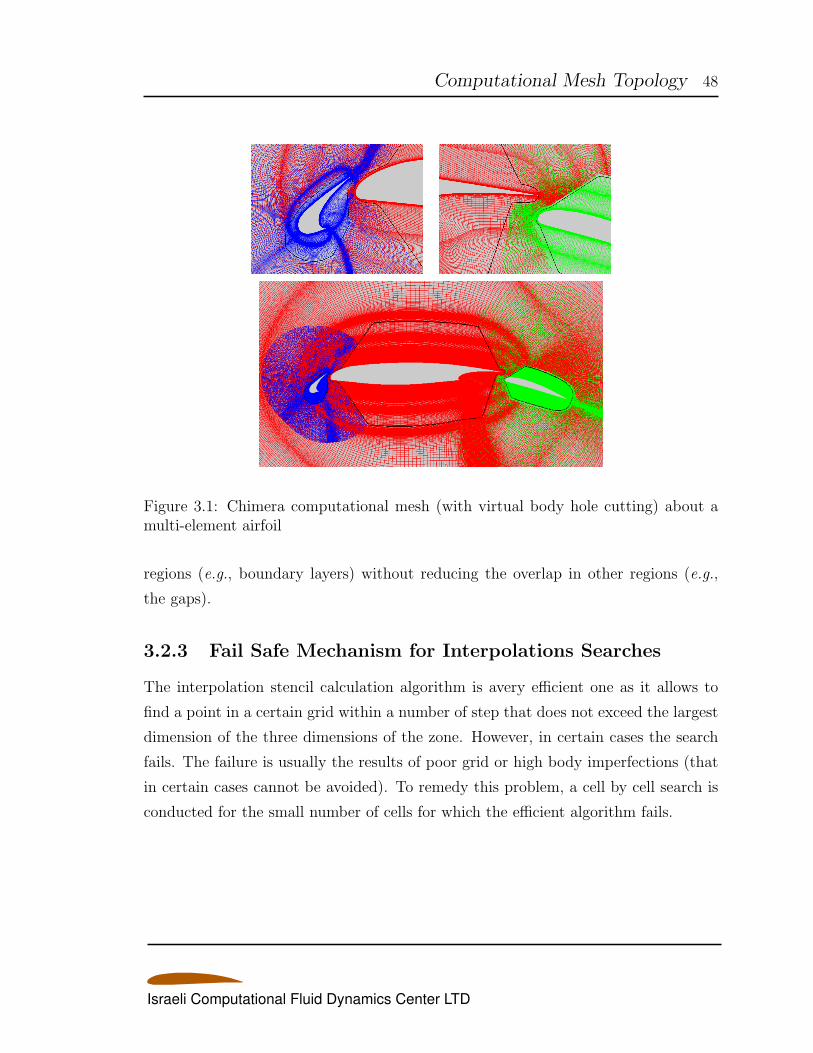
Computational Mesh Topology 48
Figure 3.1: Chimera computational mesh (with virtual body hole cutting) about amulti-element airfoil
regions (e.g., boundary layers) without reducing the overlap in other regions (e.g.,
the gaps).
3.2.3 Fail Safe Mechanism for Interpolations Searches
The interpolation stencil calculation algorithm is avery efficient one as it allows to
find a point in a certain grid within a number of step that does not exceed the largest
dimension of the three dimensions of the zone. However, in certain cases the search
fails. The failure is usually the results of poor grid or high body imperfections (that
in certain cases cannot be avoided). To remedy this problem, a cell by cell search is
conducted for the small number of cells for which the efficient algorithm fails.
Israeli Computational Fluid Dynamics Center LTD
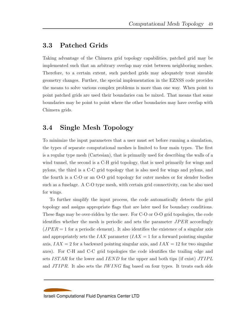
Computational Mesh Topology 49
3.3 Patched Grids
Taking advantage of the Chimera grid topology capabilities, patched grid may be
implemented such that an arbitrary overlap may exist between neighboring meshes.
Therefore, to a certain extent, such patched grids may adequately treat sizeable
geometry changes. Further, the special implementation in the EZNSS code provides
the means to solve various complex problems is more than one way. When point to
point patched grids are used their boundaries can be mixed. That means that some
boundaries may be point to point where the other boundaries may have overlap with
Chimera grids.
3.4 Single Mesh Topology
To minimize the input parameters that a user must set before running a simulation,
the types of separate computational meshes is limited to four main types. The first
is a regular type mesh (Cartesian), that is primarily used for describing the walls of a
wind tunnel, the second is a C-H grid topology, that is used primarily for wings and
pylons, the third is a C-C grid topology that is also used for wings and pylons, and
the fourth is a C-O or an O-O grid topology for outer meshes or for slender bodies
such as a fuselage. A C-O type mesh, with certain grid connectivity, can be also used
for wings.
To further simplify the input process, the code automatically detects the grid
topology and assigns appropriate flags that are later used for boundary conditions.
These flags may be over-ridden by the user. For C-O or O-O grid topologies, the code
identifies whether the mesh is periodic and sets the parameter JPER accordingly
(JPER = 1 for a periodic element). It also identifies the existence of a singular axis
and appropriately sets the IAX parameter (IAX = 1 for a forward pointing singular
axis, IAX = 2 for a backward pointing singular axis, and IAX = 12 for two singular
axes). For C-H and C-C grid topologies the code identifies the trailing edge and
sets ISTAR for the lower and IEND for the upper and both tips (if exist) JTIPL
and JTIPR. It also sets the IWING flag based on four types. It treats each side
Israeli Computational Fluid Dynamics Center LTD
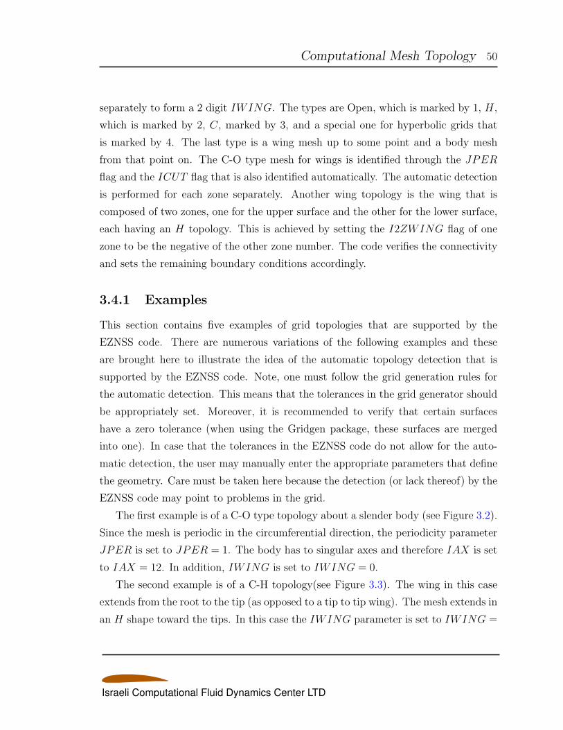
Computational Mesh Topology 50
separately to form a 2 digit IWING. The types are Open, which is marked by 1, H,
which is marked by 2, C, marked by 3, and a special one for hyperbolic grids that
is marked by 4. The last type is a wing mesh up to some point and a body mesh
from that point on. The C-O type mesh for wings is identified through the JPER
flag and the ICUT flag that is also identified automatically. The automatic detection
is performed for each zone separately. Another wing topology is the wing that is
composed of two zones, one for the upper surface and the other for the lower surface,
each having an H topology. This is achieved by setting the I2ZWING flag of one
zone to be the negative of the other zone number. The code verifies the connectivity
and sets the remaining boundary conditions accordingly.
3.4.1 Examples
This section contains five examples of grid topologies that are supported by the
EZNSS code. There are numerous variations of the following examples and these
are brought here to illustrate the idea of the automatic topology detection that is
supported by the EZNSS code. Note, one must follow the grid generation rules for
the automatic detection. This means that the tolerances in the grid generator should
be appropriately set. Moreover, it is recommended to verify that certain surfaces
have a zero tolerance (when using the Gridgen package, these surfaces are merged
into one). In case that the tolerances in the EZNSS code do not allow for the auto-
matic detection, the user may manually enter the appropriate parameters that define
the geometry. Care must be taken here because the detection (or lack thereof) by the
EZNSS code may point to problems in the grid.
The first example is of a C-O type topology about a slender body (see Figure 3.2).
Since the mesh is periodic in the circumferential direction, the periodicity parameter
JPER is set to JPER = 1. The body has to singular axes and therefore IAX is set
to IAX = 12. In addition, IWING is set to IWING = 0.
The second example is of a C-H topology(see Figure 3.3). The wing in this case
extends from the root to the tip (as opposed to a tip to tip wing). The mesh extends in
an H shape toward the tips. In this case the IWING parameter is set to IWING =
Israeli Computational Fluid Dynamics Center LTD
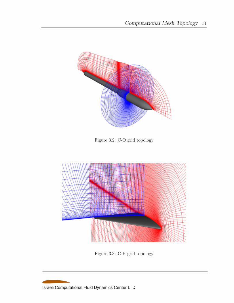
Computational Mesh Topology 51
Figure 3.2: C-O grid topology
Figure 3.3: C-H grid topology
Israeli Computational Fluid Dynamics Center LTD
Computational Mesh Topology 52
Figure 3.4: C-C grid topology
12. The IAX parameter and the JPER parameter are set to zero for this case.
The third example corresponds to a C-C type grid topology (see Figure 3.4). The
IWING parameter is set in this case to IWING = 13. In both wing cases above,
the digit “1” stand for an open tip, characteristic to wing that emanates from the
root. The digit “2” stands for the H type at the tip and the digit “3” stands for the
C type at the tip. As in the case of the C-H wing grid above, the parameters IAX
and JPER are set to zero.
The fourth and last example corresponds to the C-O type grid topology when
its used for wings (see Figure 3.5). The JPER parameter is set in this case to
JPER = 1 and the ICUT parameter is set to ICUT = 12. Depending on the
geometry, the ICUT parameter can be also set to “1” or “2.”
The fifth and last example is that of the two zone wing (see Figure 3.6). As
mentioned above it is set using the variable I2ZWING. Once verified, the program
automatically sets ISTART , IEND, JTIPL, and JTIPR.
Israeli Computational Fluid Dynamics Center LTD
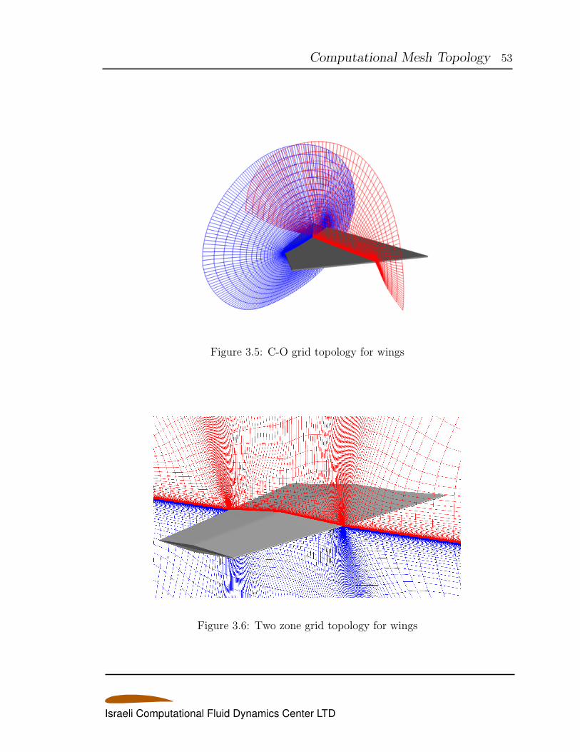
Computational Mesh Topology 53
Figure 3.5: C-O grid topology for wings
Figure 3.6: Two zone grid topology for wings
Israeli Computational Fluid Dynamics Center LTD
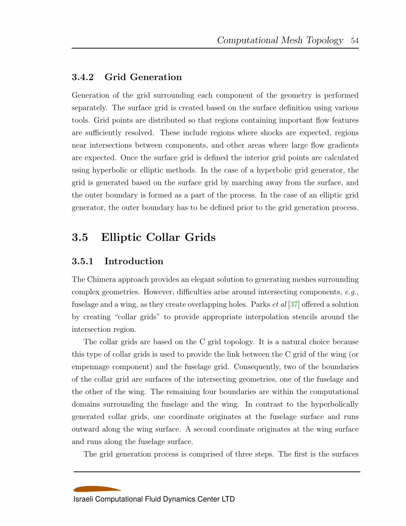
Computational Mesh Topology 54
3.4.2 Grid Generation
Generation of the grid surrounding each component of the geometry is performed
separately. The surface grid is created based on the surface definition using various
tools. Grid points are distributed so that regions containing important flow features
are sufficiently resolved. These include regions where shocks are expected, regions
near intersections between components, and other areas where large flow gradients
are expected. Once the surface grid is defined the interior grid points are calculated
using hyperbolic or elliptic methods. In the case of a hyperbolic grid generator, the
grid is generated based on the surface grid by marching away from the surface, and
the outer boundary is formed as a part of the process. In the case of an elliptic grid
generator, the outer boundary has to be defined prior to the grid generation process.
3.5 Elliptic Collar Grids
3.5.1 Introduction
The Chimera approach provides an elegant solution to generating meshes surrounding
complex geometries. However, difficulties arise around intersecting components, e.g.,
fuselage and a wing, as they create overlapping holes. Parks et al [37] offered a solution
by creating “collar grids” to provide appropriate interpolation stencils around the
intersection region.
The collar grids are based on the C grid topology. It is a natural choice because
this type of collar grids is used to provide the link between the C grid of the wing (or
empennage component) and the fuselage grid. Consequently, two of the boundaries
of the collar grid are surfaces of the intersecting geometries, one of the fuselage and
the other of the wing. The remaining four boundaries are within the computational
domains surrounding the fuselage and the wing. In contrast to the hyperbolically
generated collar grids, one coordinate originates at the fuselage surface and runs
outward along the wing surface. A second coordinate originates at the wing surface
and runs along the fuselage surface.
The grid generation process is comprised of three steps. The first is the surfaces
Israeli Computational Fluid Dynamics Center LTD
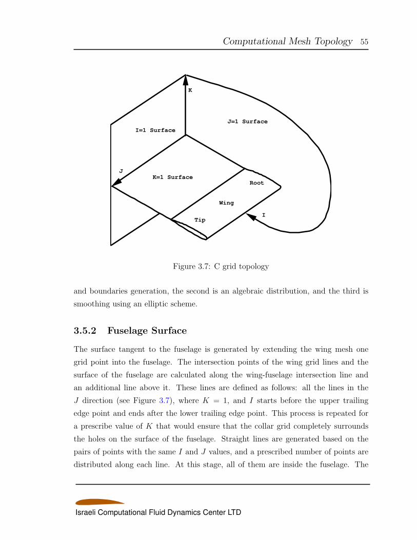
Computational Mesh Topology 55
K
J
Wing
J=1 Surface
K=1 Surface
I=1 Surface
Root
TipI
Figure 3.7: C grid topology
and boundaries generation, the second is an algebraic distribution, and the third is
smoothing using an elliptic scheme.
3.5.2 Fuselage Surface
The surface tangent to the fuselage is generated by extending the wing mesh one
grid point into the fuselage. The intersection points of the wing grid lines and the
surface of the fuselage are calculated along the wing-fuselage intersection line and
an additional line above it. These lines are defined as follows: all the lines in the
J direction (see Figure 3.7), where K = 1, and I starts before the upper trailing
edge point and ends after the lower trailing edge point. This process is repeated for
a prescribe value of K that would ensure that the collar grid completely surrounds
the holes on the surface of the fuselage. Straight lines are generated based on the
pairs of points with the same I and J values, and a prescribed number of points are
distributed along each line. At this stage, all of them are inside the fuselage. The
Israeli Computational Fluid Dynamics Center LTD
Computational Mesh Topology 56
points are then projected onto the surface of the fuselage. The projection process is
similar to finding the intersection between a line and a surface and is described below.
By choosing an exponential distribution function, the points on the defined surface
are clustered toward the wing-fuselage intersection.
3.5.3 Intersection Between a Line and a Discrete Surface
As was mentioned above, the fuselage surface is comprised of a series of grid points
that are the intersections between grid lines of the wing mesh and the surface of the
fuselage mesh. The intersection point can be easily found assuming both line and
surface are know analytical functions.
Let P1 = x1, y1, z1 and P2 = x2, y2, z2 be the points that define a line and
V1 and V2 be the position associated with P1 and P2 relative to zero, then the line
passing through the points is given by
Vl = tV1 + (1− t)V2 (3.1)
where −∞ < t < ∞. Let f(x, y, z) = 0 be the definition of a surface, then the
intersection between the line V and the surface f is given by f(V ) = 0. Depending
on the function f , the intersection point can be found analytically or numerically.
In our case, the fuselage is given by discrete points and therefore the intersection
point must be found numerically. An efficient method to locate the intersection point
is based on a bilinear interpolation within a cell of the fuselage mesh. Let P3, P4,
P5, and P6 be the point that define a surface cell and V3, V4, V5, and V6 be their
respective positions relative to zero, then a point in the cell is given by
Vc = s(rV3 + (1− r)V4) + (1− s)(rV5 + (1− r)V6) (3.2)
where 0 < r, s < 1.
If a line intersects a certain cell then Vl = Vc and 0 < r, s < 1. The parameters
r, s, and t can be found by the solution of the 3 × 3 system given by equations 3.1
and 3.2. If 0 < s < 1 the intersection point is between the points P1 and P2, and
Israeli Computational Fluid Dynamics Center LTD
Computational Mesh Topology 57
the intersection point is found by a linear interpolation, otherwise the point is found
through extrapolation. If r, or s are not between zero and one then the line does not
intersect the particular cell. The values of r, and s are then used to move to the next
cell and the system is solved until the intersection point is found.
3.5.4 Wing Surface
The surface tangent to the wing is generated following a similar process to that
used for generating the fuselage surface. The points that define the wing-fuselage
intersection are used together with points on the wing surface to generate the lines
that are inside or outside the wing, depending on the wing’s curvature. Points are
exponentially distributed on these lines and then projected onto the wing surface.
The surface is also extended in the ±I direction to cover the fuselage hole.
3.5.5 Volume Boundaries
The other four boundaries of the collar grid are generated based on the surface bound-
aries. The edges of two of the surfaces are normal to the fuselage and the wing surface,
respectively, and the other two are set so they smoothly close the volume covered by
the collar grid. It is achieved by using the same projection algorithms used for the
surface boundary generation.
3.5.6 Grid Generation
Once the boundaries are defined, internal points are computed through interpola-
tions based on the boundary values. The points are smoothed using an elliptic grid
generator based on the TTM algorithm [38]. The smoothing procedure is applied to
I = constant slices to ensure a smooth orthogonal mesh. Using the TTM algorithm
guarantees that in each I slice the coordinates are orthogonal and smooth. Control
functions are used to ensure a point distribution similar to that of the boundaries. The
whole process requires negligible amount of computer time since only a few iterations
are needed for convergence.
Israeli Computational Fluid Dynamics Center LTD
Computational Mesh Topology 58
The resulting collar grid is smooth and it maintains orthogonality everywhere it
is defined even in the region close to the intersection line. In addition, its points
are clustered toward the wing and the fuselage surfaces in a way that allows high
resolution of the intersection region.
3.5.7 Force and Moment Calculations
Collar grids maybe also used to calculate the force and moments of the surface grid
cells that are cut by the hole cutting procedure. A suite of routines allows to project
collar grid surfaces on to the appropriate body components and to set a special
hole array in the opposite manner. That way, a simple use of the force calculation
routines allow to add the contribution of the surfaces of the holes to the total forces
and moments.
3.6 Hyperbolic Collar Grids
In certain cases, it is beneficial to generate collar grids hyperbolically. In such cases,
the surface mesh is generated either by marching along the fuselage and wing surface
or, it is generated by the elliptic collar grid generator. A hyperbolic grid can have
either a C type topology or an O type topology. The latter is easy to generate and
handle but sometimes an O type mesh does not provide an adequate solution. On
the other hand, the C type topology for a hyperbolic collar grid dictates a somewhat
different grid topology at the fuselage side. This topology is marked by setting the
IWING parameter to “4” at the appropriate end of the wing. Figure 3.8 shows
a C type hyperbolic collar grid. The IWING parameter of this mesh is set to
IWING = 41.
Israeli Computational Fluid Dynamics Center LTD
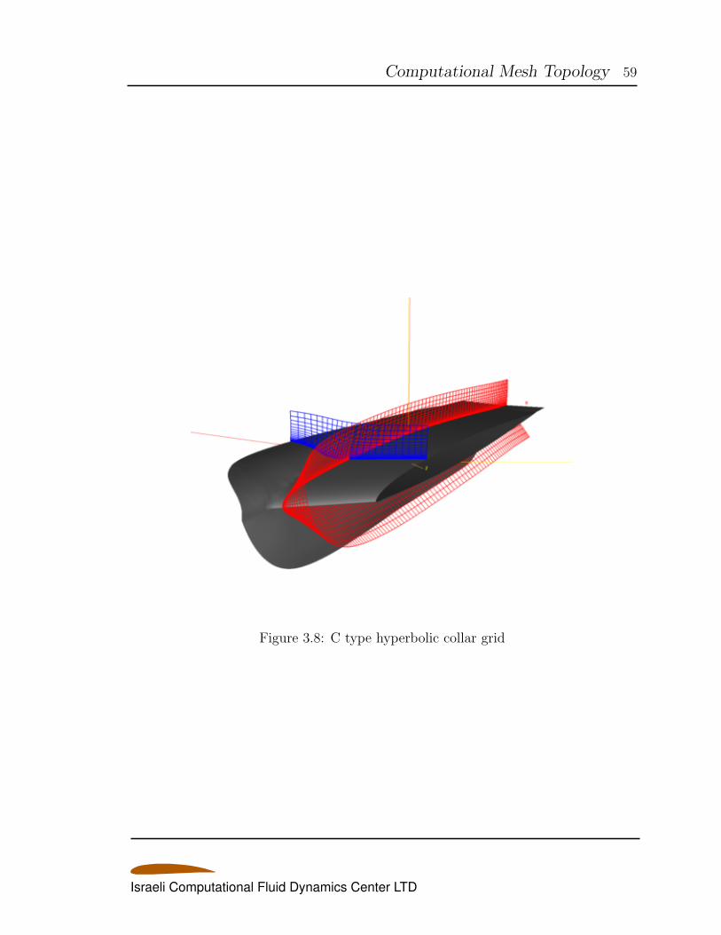
Computational Mesh Topology 59
Figure 3.8: C type hyperbolic collar grid
Israeli Computational Fluid Dynamics Center LTD
60
Chapter 4
Boundary Conditions
4.1 Introduction
Version 2.5 of the EZNSS code contains a wide variety of boundary conditions. The
boundary conditions are automatically set by the code, based on the identification of
the topology. The user may over-ride any of the boundary conditions using the input
file.
4.2 Wall Boundary Conditions
The boundary conditions applied in the inviscid, Euler equations simulations are set
to obtain a slip condition at all walls. All surfaces are assumed to be adiabatic and
the wall boundary conditions consist of an impermeable wall, with a zeroth-order zero
normal pressure gradient, and an adiabatic wall boundary condition (usually applied
at ζ = 1).
The boundary conditions applied in both laminar-flow and turbulent-flow calcu-
lations are identical and are chosen to simulate viscous flows. The wall boundary
conditions, applied at ζ = 1, enforce zero slip and adiabatic wall conditions. The
contravariant velocities U , V , W are all set to zero, and a zeroth-order zero normal
pressure gradient condition is applied.
The above conditions correspond to a non-accelerating geometry. When acceler-
Israeli Computational Fluid Dynamics Center LTD
Boundary Conditions 61
ation is apllied, to the whole geometry or parts of it, an additional term is added to
the pressure on the body, since the normal pressure gradient is not longer zero. In
such cases the pressure gradient is calculated as follows.
∂p
∂n= ρa · n (4.1)
where ρ is the fluid density, n is the normal to the geometry, and a is the acceleration.
4.3 Inflow, Outflow, and Extrapolations
The inflow boundary condition, applied at ζ = ζmax, enforces free-stream conditions,
while exit boundary conditions utilize a simple zeroth-order zero-gradient extrapola-
tion condition. In general, for all extrapolations, a zeroth-order scheme is used. This
includes the zero normal pressure gradient condition at walls.
4.3.1 Characteristic-like Inflow Outflow
To improve the inflow or boundary conditions, the characteristic relations that are
due-to Turkel have been added. For supersonic inflow, the flow quantities at the
inflow boundary (implemented in the I direction only) are set based on the current
values of the corresponding boundary. For subsonic incoming flows, the density and
velocity components are taken as the current values and the pressure is extrapolated
from the neighboring cell (zeroth order extrapolation). For supersonic outflow, all
variables are extrapolated using a zeroth order extrapolation while for subsonic flow
the outflow pressure is prescribed by the user and the density is based on the formula:
ρ1 = ρ2 +(pexit − p2)/a
22
)(4.2)
where the subscript 1 denotes the boundary and the subscript 2 denotes the neigh-
boring cell (a being the speed of sound).
The same scheme is also implemented for the K = Kmax. In that case the pro-
cedure is as follows. For each point, it is determined wether the flow is an inflow
Israeli Computational Fluid Dynamics Center LTD
Boundary Conditions 62
or outflow. Then it is determined whether it is supersonic or subsonic. And finally,
the appropriate boundary condition is applied (by setting the appropriate KOUT to
100).
4.4 Periodic Boundary Conditions
When a periodic boundary condition is required it is applied at η = ηmax, allowing
the flow to become asymmetric if warranted by the flow physics. Application of
the periodic boundary condition results in a system of periodic equations for the
respective factor. Computationally, the solution of the periodic set is very expensive
but it is necessary in order to capture asymmetric flow solutions as well as symmetric
solutions.
4.5 Cut Conditions in I Direction
The ICUT variable is used to set cut conditions in either Imin, Imax, or both. The
cut condition is employed using a simple interpolation between both sides of the cut
(taking the value from K = 2 for the interpolation.
4.6 Axis Conditions
Axis conditions can be employed at Imin or Imax, or at Kmin. The conditions in the
I direction are usually used for tips of slender bodies where the conditions in the K
direction are used for the center of tubes. The flow values at the axis are determined
by interpolation.
4.7 Symmetry Conditions
Symmetry conditions may be emplyoed in the I or J directions at each end or at
both ends. Symmetry is employed about the Y = 0 plane only and the grid must
Israeli Computational Fluid Dynamics Center LTD
Boundary Conditions 63
have a section on that plane to achieve the appropriate symmetry. For example, if
symmetry is employed at Jmin, the J = 2 section must be placed on the Y = 0 plane.
4.8 Free Stream Conditions
Free stream conditions may be employed on any boundary surface. In the current
version, nothing is set and therefore the free stream conditions remain the same. The
free stream flags may be used to turn off zonal boundary conditions on the appropriate
faces. Future versions may include the capability to change the free stream conditions
during restart.
4.9 Inlet Conditions
Inlet conditions are available in the I direction where the surface is primary aligned
with the X direction. The inlet conditions are implemented through charcteristic
relations.
4.10 Zonal Boundary Conditions
Zonal boundary conditions are handled in an automatic manner. The EZNSS code
includes a suite of routines to calculate inter grid communications. These routines
are invoked every time the configuration experiences a geometry change. All inner
boundaries (holes edges), and outer boundaries (usually at ζ = ζmax) are updated
using a tri-linear interpolation.
Israeli Computational Fluid Dynamics Center LTD
64
Chapter 5
Six Degrees of Freedom Simulation
The flow equations solved by the EZNSS code are written in an inertial coordinate
system (the computational meshes may move but the observer is set). Therefore,
the forces and moments that are calculated about bodies are forces and moments in
a Cartesian coordinate system, with its origin set in a predefined static position in
space. In the beginning of the flow simulations, it is usually attached to the aircraft
tip (or, in the case of a free stream simulation about a certain store to its tip). For
further simplification of the motion calculation, the aerodynamic forces and moments
are calculated about a reference point that is the store center of gravity. Since the
aerodynamic coefficients are given in a Cartesian coordinate system, the translational
equation of motion is formulated and solved in the Cartesian coordinate system.
Solving the rotational equation of motion in such coordinates is far more compli-
cated due to the need to recalculate the moment of inertia matrix with each rotation
of the body. It is then opted to solve the rotational equation of motion in body coor-
dinates. In what follows, the numerical solution procedure of the equation of linear
motion and of the rotational equation of motion is described.
5.1 Translational Equation of Motion
The translational equation of motion is obtained by applying Newton’s law of motion.
Since it is assumed that the mass of an aircraft or its stores remain constant, the law
Israeli Computational Fluid Dynamics Center LTD
Six Degrees of Freedom Simulation 65
takes the form:
∑F = m
dV
dt(5.1)
where∑F is the sum of forces (aerodynamic and other) acting on the body, m is
the mass of the store, and V is the velocity vector. The translational velocity of a
certain store at a time step n+ 1 is calculated using forward differences arriving at:
V n+1 = V n +∆t
m
(3
2
∑F n − 1
2
∑F n−1
)(5.2)
The motion increment is then evaluated using
∆X = ∆t
(V n+1 + V n
)2
(5.3)
The motion increment is applied at the center of gravity of the corresponding body.
In practice, this means that every grid point is translated by ∆X.
5.2 Rotational Equation of Motion
The rotational equation of motion is obtained by applying Newton’s second law for
angular motion. Once again, it is assumed that the geometry of a parent aircraft
and any of its stores remain constant and therefore, one may assume that the iner-
tia matrix remains unchanged as well. The rotational equation of motion in body
coordinates takes the form:
∑M = I
dΩ
dt+ Ω× H (5.4)
where∑M is the sum of moments, I is the moment of inertia matrix, Ω is the angular
velocity vector, and H is the angular momentum vector. The aerodynamic moments,
Israeli Computational Fluid Dynamics Center LTD
Six Degrees of Freedom Simulation 66
evaluated in Cartesian coordinates, are transformed into body coordinates using:
M1
M2
M3
=
cosψ cos θ sinψ cos θ − sin θ(cosψ sin θ sinϕ
− sinψ cosϕ
) (sinψ sin θ sinϕ
+cosψ cosϕ
)cos θ sinϕ(
cosψ sin θ cosϕ
+sinψ sinϕ
) (sinψ sin θ cosϕ
− cosψ sinϕ
)cos θ cosϕ
Mx
My
Mz
(5.5)
In addition to the above mentioned assumptions, it is further assumed that a
typical store has at least one symmetry plane. In its local coordinates, out of the
three off-diagonal terms, Ixz is allowed to be non-zero. The other two terms Ixy and
Iyz must be zero. In light of this simplification, the angular acceleration may be
calculated by: p
q
r
=
M1−(r+pq)Ixz−qr(Iz−Iy)
IxM2−(r2−p2)Ixz−pr(Ix−Iz)
IyM3−(p−qr)Ixz−pq(Iy−Ix)
Iz
(5.6)
where p, q, and r are the angular velocity components in body coordinates. The
angular velocity of a certain store at a time step n+1 is also calculated using forward
differences arriving at:pn+1
qn+1
rn+1
=
pn
qn
rn
+∆t
3
2
pn
qn
rn
− 1
2
pn−1
qn−1
rn−1
(5.7)
The angular velocities in Cartesian coordinates (ψ, θ, and ϕ) may be calculated using
the angular velocities in body coordinates (p, q, and r) by applying the following
transformation: ψ
θ
ϕ
=
q sinϕcos θ
+ r cosϕcos θ
q cosϕ− r sin θ
p+ q sinϕ tan θ + r cosϕ tan θ
(5.8)
Israeli Computational Fluid Dynamics Center LTD
Six Degrees of Freedom Simulation 67
5.2.1 Quaternions
Euler angles present the well-know pitch singularity. When the angle θ approaches
values of θ = ±90 attitude errots become noticeable. To resolve this difficulty,
quaternions have been introduced into the 6 degrees of freedom simulation. The
quaternion consists of four parameters: a scalar (q0), and a vector (q1,q2,q3). An
extra constraint is required, q20 + q21 + q22 + q23 = 1. This constraint can be easily
enforced through a normalization. Quaternion update is conducted through four first
order differential equations as follows:q0
q1
q2
q3
= −1
2
0 p q r
−p 0 −r q
−q r 0 −p−r −q p 0
q0
q1
q2
q3
(5.9)
Users may choose whether to use quaternions or Euler angles. When quaternions are
chosen the Euler angles are used just for presentation of the simulation results.
5.3 Store Location Update
Following the solution of the translational equation of motion and the rotational
equation of motion, the position and attitude of the store may be updated using the
relations:
xn+1cg = xncg +∆x
yn+1cg = yncg +∆y
zn+1cg = zncg +∆z
ψn+1 = ψn +∆t ψ
θn+1 = θn +∆t θ
ϕn+1 = ϕn +∆t ϕ (5.10)
Israeli Computational Fluid Dynamics Center LTD
Six Degrees of Freedom Simulation 68
where ψ, θ, ϕ, are evaluated using
ψ =ψn+1 + ψn
2
θ =θn+1 + θn
2
ϕ =ϕn+1 + ϕn
2(5.11)
The new grid location of a certain store is obtained by applying the above relations
to each grid point. The application of the rotation is conducted about the center of
gravity of the store.
Israeli Computational Fluid Dynamics Center LTD
69
Chapter 6
Static and Dynamic Aeroelasticity
Solution of the discrete aeroelastic equation of motion, for a structural large model,
can be computationally burdensome. As a result, there is a motivation to reduce
the size of the problem without sacrificing significant accuracy. One approach to
reduce the computational burden of FEM-based aeroelastic analysis is to represent
the structural displacements as a linear combination of a set of its modes of vibration,
as given by:
u =[ΦR ΦE
] ξR
ξE
(6.1)
In this case,[ΦR] represents the rigid-body modes, and [ΦE] represents a subset of
the elastic modes of vibration. Both [ΦR] and [ΦE], along with their corresponding
natural frequencies, ωi, are solutions to the eigenvalue problem of the free vibration
of the structure, which is given by:
([K]− ω2
i [M ])Φi = 0 (6.2)
By utilizing such a decomposition, the size of the aeroelastic problem reduces to the
number of modes picked up. Typically, a few tens of modes are sufficient to represent
displacements of a full aircraft configuration, which, in the FEM, may involve hundred
thousands degrees of freedom.
The EZNSS code utilizes a modal structural model for interfacing the flow solver
Israeli Computational Fluid Dynamics Center LTD
Static and Dynamic Aeroelasticity 70
and structural models, for calculating elastic shape deformations, and applying them
to the computational mesh. It utilizes two forms of aeroelastic displacements, a
simple rigid displacement of the whole mesh and a deformation that is based on
trans-finite interpolations. This chapter briefly describes the models for static and
dynamic aeroelasticity and the TFI approach.
6.1 Static Aeroelasticity
The modal approach to static aeroelasticity assumes that the elastic deformations of
the aircraft structure under external loads can be described as a linear combination
of a set of low-frequency elastic mode shapes [ϕE], typically 10 to 30, namely
uE = [ϕE]ξE (6.3)
where ξE is the generalized elastic displacement vector. The resulting static equi-
librium equation in generalized coordinates is:
[KE]ξE = FE (6.4)
where [KE] is the generalized stiffness matrix associated with [ϕE], and FE is the
associated generalized aerodynamic force vector. Orthogonality of the rigid-body and
elastic modes with respect to the structural mass and stiffness matrices implies that
[KE] is diagonal and that inertia relief effects in the right hand side of Eq. (6.4) are
taken care of automatically. The rigid-body counterpart of Eq. (6.4) is used below
in the maneuver trim process.
The generalized forces in Eq. (6.4) are obtained by
FE = [ϕA]T (FA − FC) (6.5)
where FA is the aerodynamic force vector at the aerodynamic surface grid points,
FC is the aerodynamic force vector associated with the reference aerodynamic
shape, and [ϕA] is the elastic modes matrix, expressed at the aerodynamic inter-
Israeli Computational Fluid Dynamics Center LTD
Static and Dynamic Aeroelasticity 71
face grid points as described below. It is assumed that the reference loads vector
FC has been defined in a previous aerodynamic analysis. This is the case when
the reference aerodynamic shape is the “cruise shape”, namely the shape designed
for best aerodynamic performance at nominal cruise conditions. The reference aero-
dynamic shape can also be defined as the “jig shape”, namely the unstressed shape,
for which FC = 0.
Using the modal approach, the modal stiffness matrix and the modes matrix are
the only structural data required for the maneuver load analysis. These matrices are
calculated by the finite element code, and are read in the CFD run as it starts, and
after each structural optimization run. Since the number of structural modes used
is typically small (in this work 15 structural modes were found to be conservatively
sufficient) very little structural data is required to be transferred.
6.2 Equations of Motion for Uncoupled Aeroelas-
tic Motion
The equations of motion corresponding to an uncoupled aeroelastic motion, given in
generalized coordinates as:
[Mii]ξ+[2ζMii
√Ωi
]ξ+ [MiiΩi] ξ = F (t) (6.6)
where M is the diagonal, generalized-mass matrix, Ωi are the eigenvalues, ζ is the
structural damping coefficient, ξ is the vector of generalized displacements, and F are
the aerodynamic generalized forces.
6.2.1 Numerical Scheme
Since the generalized mass matrix is diagonal, the modes are uncoupled and the time
integration of the differential equation can be performed for each mode separately.
Finite differences are used to evaluate the time derivatives of ξ. In addition, the
equations are put in delta form so that only the increments are taken into account.
Israeli Computational Fluid Dynamics Center LTD
Static and Dynamic Aeroelasticity 72
This results in the following set of equations:
∆ξi + 2ζ√
Ωi∆ξi + Ωi∆ξi =∆Fi
Mii
(6.7)
one equation for each mode.
6.2.2 Solution Method
Prior to numerically solving the modal equations of motion, the system is rewritten
in a state space formulation, as follows:
∆ξi = ∆ηi
∆ηi =∆Fi
Mii
− 2ζ√
Ωi∆ηi − Ωi∆ξi (6.8)
The system can now be integrated using a standard Runge-Kutta method. The
EZNSS code utilizes a 4th order Runge-Kutta scheme to advance the solution in time.
This formulation has been found very robust.
6.3 Mesh Deformations using the TFI Approach
The TFI approach utilized in the EZNSS code is an arc-length TFI. In this approach,
the grid coordinates are parameterized by the length of the coordinates in three
directions. In each direction, the parameterization results in an array whose values
extend between 0.0, at the beginning of the line and 1.0 at the end of the line. The
arrays for the I direction, the J direction and the K direction are marked by P ξ, P η,
and P ζ , respectively.
A volume grid in constrained by 6 faces. Each of the faces is constrained by 4
edges and each edge is constrained by to vertices. To deform a volume grid, the edge
deformations are set, then the face deformations and finally, the face deformations
are used as the input to the three-dimensional TFI procedure.
Israeli Computational Fluid Dynamics Center LTD
Static and Dynamic Aeroelasticity 73
6.3.1 Face Deformations
The typical computational mesh that is used in the CFD computations is a body-
fitted, curvilinear mesh transformed from the physical space into a Cartesian com-
putational space. This transformation is provided as a part of the input to the CFD
program (the mesh itself is already given in the Cartesian computational space). The
transformation brings the body surface onto one computational plane, referred to
here, as the K = 1 face. The next face is found at the opposite end of the com-
putational space and is called the K = Kdim face. The other faces are the I = 1
face, the I = Idim face, the J = 1 face, and the J = Jdim face. Depending on the
mesh topology, the body surface may fill up the whole K = 1 face or just a part of it.
For example, in the case of the C-H type topology that is used for wings, the body
surface extends only between the left and right wing tips and from the leading edge
and trailing edge. Figure 6.1 shows a schematic of the computational space and the
body surface. The deformations of the body surface grid points are obtained using
the modal approach. The rest of the K = 1 face are calculated based on the surface
grid points by imposing smooth grid lines throughout the surface.
Once the K = 1 face grid points deformations are set the rest of the face are
deformed as follows. The K = Kdim face deformations are set to be equal to the
K = 1 face. Then deformations at the edges connecting between the K = 1 face and
the K = Kdim face are calculated using a one-dimensional TFI. In the K direction
the one-dimensional TFI for the ∆X deformations takes the form:
∆Xi,j,k =(1− P ζ
i,j,k
)∆Xij1 + P ζ
i,j,k∆Xi,j,Kdim (6.9)
Next, the deformations of the other faces are calculated using a two-dimensional TFI.
The formula for the ∆X deformations on the I = Idim face takes the form:
∆X1,j,k = A1,j,k∆X1,j,1 +B1,j,k∆X1,j,Kdim
C1,j,k∆X1,1,k +D1,j,k∆X1,Jdim,k
−A1,j,kC1,j,k∆X1,1,1 −B1,j,kC1,j,k∆X1,1,Kdim
−A1,j,kD1,j,k∆X1,Jdim,1 −B1,j,kC1,j,k∆X1,Jdim,Kdim (6.10)
Israeli Computational Fluid Dynamics Center LTD
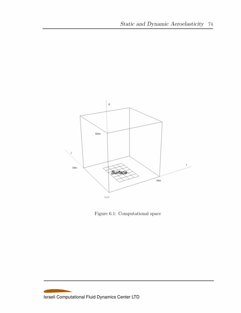
Static and Dynamic Aeroelasticity 74
Figure 6.1: Computational space
Israeli Computational Fluid Dynamics Center LTD
Static and Dynamic Aeroelasticity 75
The blending functions, A, B, C, and D are given by:
Ai,j,k = 1− ηi,j,k
Bi,j,k = ηi,j,k
Ci,j,k = 1− ξi,j,k
Di,j,k = ξi,j,k (6.11)
and
ξ =P η1,j,1 + P ζ
1,1,k
(P η1,j,Kdim − P η
1,j,1
)P1,j,k
η =P ζ1,1,k + P η
1,j,1
(P η1,Jdim,k − P η
1,1,k
)P1,j,k
P1,j,k = 1−(P η1,j,Kdim − P η
1,j,1
) (P ζ1,Jdim,k − P ζ
1,1,k
)(6.12)
6.3.2 Volume Deformations
The face deformations are used as the input to the three-dimensional TFI whose
formula is given by:
∆Xi,j,k = V 1 + V 2 + V 3− V 12− V 13− V 23 + V 123 (6.13)
Israeli Computational Fluid Dynamics Center LTD
Static and Dynamic Aeroelasticity 76
where
V 1 =(1− P ξ
i,j,k
)∆X1,j,k + P ξ
i,j,k∆XIdim,j,k
V 2 =(1− P η
i,j,k
)∆Xi,1,k + P η
i,j,k∆Xi,Jdim,k
V 3 =(1− P ζ
i,j,k
)∆Xi,j,1 + P ζ
i,j,k∆Xi,j,Kdim
V 12 =(1− P ξ
i,j,k
) (1− P η
i,j,k
)∆X1,1,k +
(1− P ξ
i,j,k
)P ηi,j,k∆X1,Jdim,k
+ P ξi,j,k
(1− P η
i,j,k
)∆XIdim,1,k + P ξ
i,j,kPηi,j,k∆XIdim,Jdim,k
V 13 =(1− P ξ
i,j,k
)(1− P ζ
i,j,k
)∆X1,j,1 +
(1− P ξ
i,j,k
)P ζi,j,k∆X1,j,Kdim
+ P ξi,j,k
(1− P ζ
i,j,k
)∆XIdim,j,1 + P ξ
i,j,kPζi,j,k∆XIdim,j,Kdim
V 23 =(1− P η
i,j,k
) (1− P ζ
i,j,k
)∆Xi,1,1 +
(1− P η
i,j,k
)P ζi,j,k∆Xi,1,Kdim
+ P ηi,j,k
(1− P ζ
i,j,k
)∆Xi,Jdim,1 + P η
i,j,kPζi,j,k∆Xi,Jdim,Kdim
V 123 =(1− P ξ
i,j,k
) (1− P η
i,j,k
) (1− P ζ
i,j,k
)∆X1,1,1
+(1− P ξ
i,j,k
) (1− P η
i,j,k
)P ζi,j,k∆X1,1,Kdim
+(1− P ξ
i,j,k
)P ηi,j,k
(1− P ζ
i,j,k
)∆X1,Jdim,1
+ P ξi,j,k
(1− P η
i,j,k
) (1− P ζ
i,j,k
)∆XIdim,1,1
+(1− P ξ
i,j,k
)P ηi,j,kP
ζi,j,k∆X1,Jdim,Kdim
+ P ξi,j,k
(1− P η
i,j,k
)P ζi,j,k∆XIdim,1,Kdim
+ P ξi,j,kP
ηi,j,k
(1− P ζ
i,j,k
)∆XIdim,Jdim,1
+ P ξi,j,kP
ηi,j,kP
ζi,j,k∆XIdim,Jdim,Kdim (6.14)
Following the volume mesh deformations calculation, the mesh is updated using a
simple addition using:
Xi,j,k = Xi,j,k +∆Xi,j,k
Yi,j,k = Xi,j,k +∆Yi,j,k
Zi,j,k = Xi,j,k +∆Zi,j,k (6.15)
Israeli Computational Fluid Dynamics Center LTD
77
Chapter 7
Parallelization
7.1 Introduction
Parallel computer architectures are an essential tool in simulating the flow about
complex aircraft configurations, especially when the flow is unsteady or when the
geometry changes. The ever growing computational meshes and the accompanying
vast amount of numerical operations require the use of parallel processing. Current
applications utilize shared and distributed memory architectures along with the ap-
propriate application program interface (API). The OpenMP API [39] was introduced
as an industry standard to support shared memory programs with simple directives.
Simple directives facilitate the loop level parallelism. The message passing interface
(MPI) [40] is an example of the support of distributed memory programming. An-
other example is the parallel virtual machine (PVM). [41] In contrast to the shared
memory architecture, distributed memory requires to hand-write pieces of code to
facilitate the parallel processing.
The OpenMP programming paradigm provides the means to easily introduce par-
allelism when developing new applications, or even when parallelizing an existing
code. OpenMP, however, is limited to the loop level and most compilers do not al-
low directive nesting and are thus limited to a single parallelism level. As a result,
scalability is limited and the efficiency rapidly degrades when using a large number
of processors. Moreover, even compilers that do allow the use of nested directives do
Israeli Computational Fluid Dynamics Center LTD
Parallelization 78
not automatically account for all the critical issues that arise when parallelizing an
existing code.
Scalability is mostly achieve by using application specific code and the MPI li-
braries. Besides being difficult, the use of MPI is error-prone. Furthermore, using
MPI usually requires to utilize domain decomposition methods. It is quite common
that the physical space is arbitrarily split to accommodate the parallelization. Com-
putational blocks that result from the decomposition procedure communicate with
each other using MPI to transfer data to and from the boundaries of the blocks.
When using explicit algorithms, the decomposition does not hinder the convergence
nor does it affect the development of the flow. In contrast, domain decomposition
may slow down the convergence of implicit algorithms. Furthermore, when simulating
unsteady flows, the decomposition may alter the solution behavior and accuracy.
The recent emergence of shared memory parallel architectures, such as the SGI
Altix Linux based servers, provide the means for significant scalability. However,
as mentioned above, when using single-level parallelism (with OpenMP directives),
the parallelization efficiency dramatically decreases when the number of processors
increases. In recent years, the growing interest in multi-level parallelism (MLP) re-
sulted in various strategies. From using system level calls (such as “fork” and “join”),
to hybrid approaches using MPI and OpenMP, to multiple levels of parallelism using
OpenMP only. [42] Reference [42] also includes a review of previous multi-level par-
allelism efforts. The current paper describes a new multi-level parallelism approach
that allows to use the OpenMP directives and to divide the loads between groups
of processors in such a way that the parallelization efficiency drop may be greatly
reduced. Moreover, the current approach provides the means to convert a single level
parallelism code to a multi-level parallelism code with minor changes to the original
code.
7.2 Single-Level Parallelism
Using single level OpenMP parallelism, one could either parallelize the code in the
zonal level or the loop level. Zonal level parallelism is limited since the largest number
Israeli Computational Fluid Dynamics Center LTD
Parallelization 79
of processors that may be used is the number of zones, namely one processor handles
one zone. Such a parallelization scheme is efficient only when the sizes of the zones
are similar. This rarely occurs. Moreover, quite often, the number of zones may be
small, especially when simulating simple geometries. For example, the simulation of
the flow about a wing or a simple slender body may require only one zone. And even
when the number of zones is large, a balanced load may be achieved only after several
zones are grouped together. Each group of zones is then handled by a certain single
processor.
Consequently, a scalable parallelization may be achieved only on the loop level.
Of course, one would like to parallelize the outer most loop or loops of the program,
loops that contain the bulk load of the solver. Each section of the right hand side,
namely, the inviscid section, the smoothing section (if applicable), the viscous sec-
tion, and the turbulence modeling section may be separately parallelized quite easily.
Parallelization of the left hand side, namely the inversion of the left hand side matrix,
is facilitated by the alternate direction nature of the approximate factorization (it is
in fact an ADI scheme). Following the factorization, the inversion of the matrix is re-
placed by a series of line inversions that are independent from each other. Therefore,
the parallelization of the left hand side is also easily carried out. All of the above is
conducted by a relatively small number of OpenMP directives.
The following example, taken directly from the EZNSS code, illustrates the ease
of parallelization using OpenMP directives. As explained above, the outer most loop
is parallelized to reduce the overhead and to avoid was is term as “granularity.” The
variables that are defined by the “PRIVATE” clause are multiplied during run time,
based on the number of processors that available for the specific task. The efficiency
of such parallelization depend on two factors. The first is the length of the outer
most loop with respect to the number of available processors. If the loop is short and
the number of processors does not evenly divide into the loop length, the efficiency
is expected to be low. The second factor is the amount of work that is conducted
in the inner most loop. A small amount of work, compared to the whole program,
would result in low efficiency. High efficiency may be achieved only when both factors
favorably affect the parallelization.
Israeli Computational Fluid Dynamics Center LTD
Parallelization 80
C$OMP PARALLEL DO PRIVATE(I,J,K,WA,A,B,C,WA0,WA1,WA2,WA3,WA4)
C$OMP& SHARED(MDIM,IDIM,JDIM,KDIM,IB,IE,IVIS)
DO K=KB,KE
DO J=JB,JE
DO I=IB,IE
....
Some work
....
END DO
END DO
END DO
C$OMP END PARALLEL DO
Consequently, as mentioned above, the efficiency of the loop level parallelism drops
when using a large number of processors. The reason is two-fold: first, certain proces-
sors have to access the memory that resides in another node that may be physically
further away; and second, the remainder of a loop may become significant. For ex-
ample, when a loop of the size of 50 is parallelized and 16 processors are used, 14 of
the processors may wait for the completion of the last 2.
7.3 Multi-Level Parallelism
The ideal solution would be to use zonal parallelization along with loop level par-
allelization. Such an ideal solution would utilize OpenMP directives. The choice of
OpenMP is due to its aforementioned simplicity. However, not all compilers support
the nesting of parallel constructs in OpenMP. Moreover, even the compilers that do
allow to have nested directives, do not always account for the appropriate duplication
of works arrays (through the “PRIVATE” directive). The recent version of the Intel
Fortran compiler allows the nesting of OpenMP directives and it is the one that is
used in the current work. [43]
The first part of the multi-level parallelization entails the grouping of the zones
into groups as prescribed by the user. This is the outer parallelization level. Splitting
Israeli Computational Fluid Dynamics Center LTD
Parallelization 81
into groups that would have an approximately balanced computational load may be
achieved by using a rather simple algorithm. The second part has already existed in
the code, namely the loop level parallelism. All that is left to do is to add a few more
directives to set the nested parallelism, to prescribe the number of groups, and to
prescribe the number of threads for each group (the total number of processors being
the number of groups times the number of threads).
As mentioned above, not all compilers fully account for the need to duplicate work
arrays and temporary variables. Since the number of total processors and the amount
of required memory space are known, one could allocated the appropriate amount of
memory and to set the memory for each group or thread as needed.
The following example illustrates the introduction of multi level parallelism into
the EZNSS code. The original single level code had a simple loop for solving the flow
in all the zones as follows:
! Zonal loop
DO N = 1, NZ
....
SOLVER
....
END DO
! End zonal loop
The flow solver part was parallelized exactly as described in the previous section.
As mentioned above, to achieve a balanced multi level parallelism, the zones have
to be grouped where each of the groups has a comparable computational load. In
the development process, it was found that the computational time per grid point
grows as the zone becomes larger. Therefore a weighing strategy was adopted as a
part of the grouping algorithm. The number of zones per each group is stored in an
appropriate array and another array stores the list of zones that belong to each groups.
The following code shows how the arrays are utilized to determine the appropriate
zone for each outer level. The SOLVER part remains parallelized as described above
as it comprises the inner parallelization level. The rest of the changes are OpenMP
Israeli Computational Fluid Dynamics Center LTD
Parallelization 82
calls and directives that are used to enable nested parallelism, to set the number of
threads for each level, and to actually parallelize the outer loop. The number of total
threads is of course MLPOUTER * MLPINNER.
! Start of multi level parallelism section
CALL OMP_SET_NESTED(.TRUE.)
! Outer parallelization level
CALL OMP_SET_NUM_THREADS(MLPOUTER)
!$OMP PARALLEL DO PRIVATE(NMLP,IMEM,N)
DO NMLP = 1, MLPOUTER
CALL OMP_SET_NUM_THREADS(MLPINNER)
DO IMEM = 1, IGRPSIZE(NMLP)
N = IGRPMEMS(NMLP,IMEM)
....
SOLVER
....
END DO
! End zonal loop
END DO
C$OMP END PARALLEL DO
!End group
Ideally, the above code should have been sufficient to accommodate the MLP scheme.
However, the Intel compiler, does not multiply work arrays twice. Fortunately, this
deficiency does not present a major obstacle. Since the user has to prescribe the
number of inner and outer threads, the total number of processors is known and
therefore the exact size of the work arrays is also known. These are allocated and
appropriately transferred to each of the groups. They are later multiplied by the
OpenMP directives of the inner parallelization level. Thus the SOLVER part remains
unchanged.
Israeli Computational Fluid Dynamics Center LTD
83
Chapter 8
Summary
This version of the manual is the first one that contains a user manual and a partial
test case description. This version of the code contains many of the long waited fea-
tures such as store separation from a pivot release point, a line Gauss-Seidel marching
scheme, Spalart-Allmaras and k− ω-SST turbulence model, and an embedded spline
capability. As the code is still being developed, with a long list of feature requests,
new versions with new features shall be available in the near future.
Israeli Computational Fluid Dynamics Center LTD
84
Appendix A
Jacobian Matrices
A.1 Inviscid Flux Vectors Jacobian Matrices
A, B, C =
kt kx ky kz 0
kxϕ2 − uθ kt + θ − kxγ2u kyu− γ1kxv kzu− γ1kxw kxγ1
kyϕ2 − vθ kxv − kyγ1u kt + θ − kyγ2v kzv − γ1kyw kyγ1
kzϕ2 − wθ kxw − kzγ1u kyw − kzγ1v kt + θ − kzγ2w kzγ1
θ(2ϕ2 − γeρ) kxβ − γ1uθ kyβ − γ1vθ kzβ − γ1wθ kt + γθ
(A.1)
where
ϕ2 = 0.5(γ − 1)(u2 + v2 + w2)
θ = kxu+ kyv + kzw
γ1 = γ − 1
γ2 = γ − 2
β =γe
ρ− ϕ2
with k = ξ to obtain A, k = η to obtain B, and k = ζ to obtain C.
Israeli Computational Fluid Dynamics Center LTD
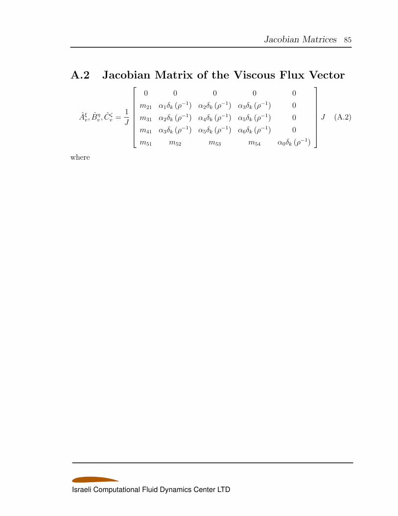
Jacobian Matrices 85
A.2 Jacobian Matrix of the Viscous Flux Vector
Aξv, B
ηv , C
ζv =
1
J
0 0 0 0 0
m21 α1δk (ρ−1) α2δk (ρ
−1) α3δk (ρ−1) 0
m31 α2δk (ρ−1) α4δk (ρ
−1) α5δk (ρ−1) 0
m41 α3δk (ρ−1) α5δk (ρ
−1) α6δk (ρ−1) 0
m51 m52 m53 m54 α0δk (ρ−1)
J (A.2)
where
Israeli Computational Fluid Dynamics Center LTD
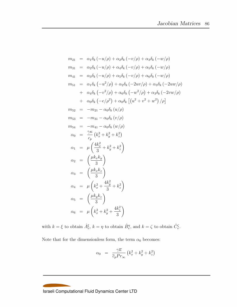
Jacobian Matrices 86
m21 = α1δk (−u/ρ) + α2δk (−v/ρ) + α3δk (−w/ρ)
m31 = α2δk (−u/ρ) + α4δk (−v/ρ) + α5δk (−w/ρ)
m41 = α3δk (−u/ρ) + α5δk (−v/ρ) + α6δk (−w/ρ)
m51 = α1δk(−u2/ρ
)+ α2δk (−2uv/ρ) + α3δk (−2uw/ρ)
+ α4δk(−v2/ρ
)+ α6δk
(−w2/ρ
)+ α3δk (−2vw/ρ)
+ α0δk(−e/ρ2
)+ α0δk
[(u2 + v2 + w2
)/ρ]
m52 = −m21 − α0δk (u/ρ)
m53 = −m31 − α0δk (v/ρ)
m54 = −m41 − α0δk (w/ρ)
α0 =γκ
cp
(k2x + k2y + k2z
)α1 = µ
(4k2x3
+ k2y + k2z
)α2 =
(µkxky3
)α3 =
(µkxkz3
)α4 = µ
(k2x +
4k2y3
+ k2z
)α5 =
(µkykz3
)α6 = µ
(k2x + k2y +
4k2z3
)
with k = ξ to obtain Aξv, k = η to obtain Bη
v , and k = ζ to obtain Cζv .
Note that for the dimensionless form, the term α0 becomes:
α0 =γκ
cpPr∞
(k2x + k2y + k2z
)
Israeli Computational Fluid Dynamics Center LTD
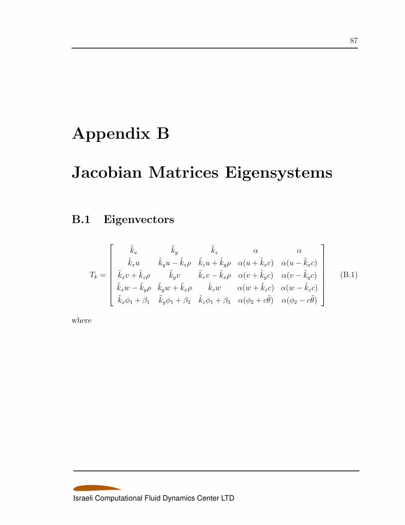
87
Appendix B
Jacobian Matrices Eigensystems
B.1 Eigenvectors
Tk =
kx ky kz α α
kxu kyu− kzρ kzu+ kyρ α(u+ kxc) α(u− kxc)
kxv + kzρ kyv kzv − kxρ α(v + kyc) α(v − kyc)
kxw − kyρ kyw + kxρ kzw α(w + kzc) α(w − kzc)
kxϕ1 + β1 kyϕ1 + β2 kzϕ1 + β3 α(ϕ2 + cθ) α(ϕ2 − cθ)
(B.1)
where
Israeli Computational Fluid Dynamics Center LTD
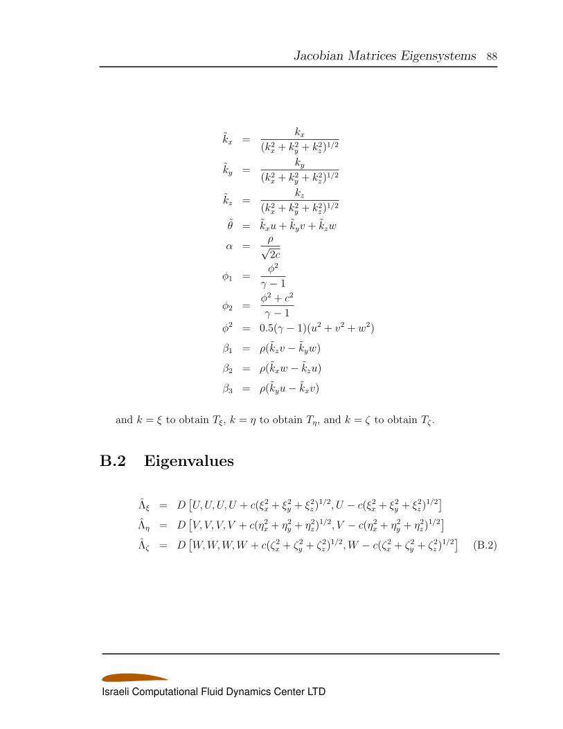
Jacobian Matrices Eigensystems 88
kx =kx
(k2x + k2y + k2z)1/2
ky =ky
(k2x + k2y + k2z)1/2
kz =kz
(k2x + k2y + k2z)1/2
θ = kxu+ kyv + kzw
α =ρ√2c
ϕ1 =ϕ2
γ − 1
ϕ2 =ϕ2 + c2
γ − 1
ϕ2 = 0.5(γ − 1)(u2 + v2 + w2)
β1 = ρ(kzv − kyw)
β2 = ρ(kxw − kzu)
β3 = ρ(kyu− kxv)
and k = ξ to obtain Tξ, k = η to obtain Tη, and k = ζ to obtain Tζ .
B.2 Eigenvalues
Λξ = D[U,U, U, U + c(ξ2x + ξ2y + ξ2z )
1/2, U − c(ξ2x + ξ2y + ξ2z )1/2]
Λη = D[V, V, V, V + c(η2x + η2y + η2z)
1/2, V − c(η2x + η2y + η2z)1/2]
Λζ = D[W,W,W,W + c(ζ2x + ζ2y + ζ2z )
1/2,W − c(ζ2x + ζ2y + ζ2z )1/2]
(B.2)
Israeli Computational Fluid Dynamics Center LTD
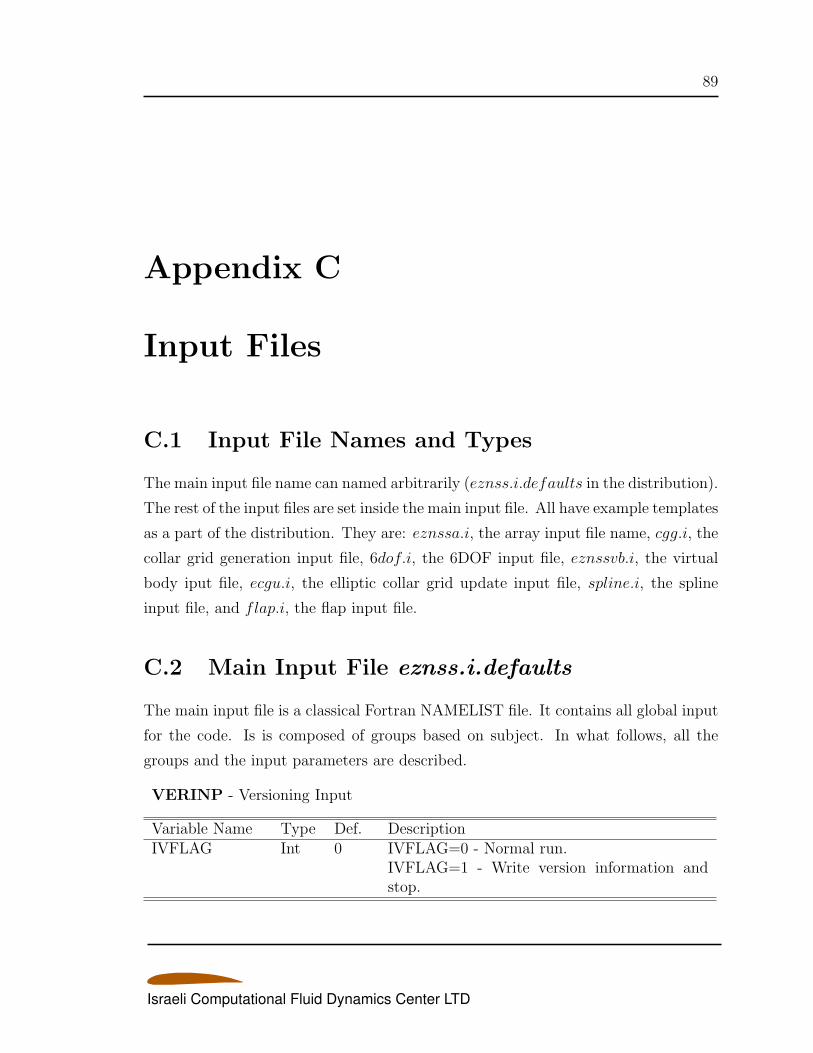
89
Appendix C
Input Files
C.1 Input File Names and Types
The main input file name can named arbitrarily (eznss.i.defaults in the distribution).
The rest of the input files are set inside the main input file. All have example templates
as a part of the distribution. They are: eznssa.i, the array input file name, cgg.i, the
collar grid generation input file, 6dof.i, the 6DOF input file, eznssvb.i, the virtual
body iput file, ecgu.i, the elliptic collar grid update input file, spline.i, the spline
input file, and flap.i, the flap input file.
C.2 Main Input File eznss.i.defaults
The main input file is a classical Fortran NAMELIST file. It contains all global input
for the code. Is is composed of groups based on subject. In what follows, all the
groups and the input parameters are described.
VERINP - Versioning Input
Variable Name Type Def. DescriptionIVFLAG Int 0 IVFLAG=0 - Normal run.
IVFLAG=1 - Write version information andstop.
Israeli Computational Fluid Dynamics Center LTD
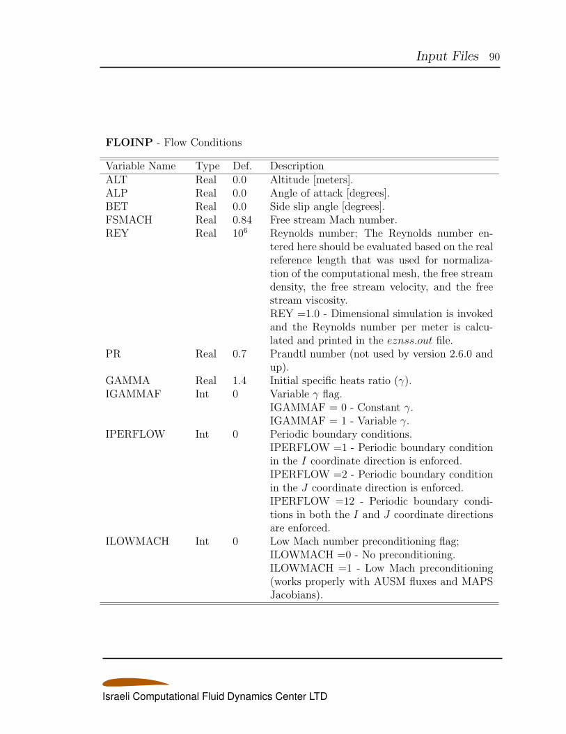
Input Files 90
FLOINP - Flow Conditions
Variable Name Type Def. DescriptionALT Real 0.0 Altitude [meters].ALP Real 0.0 Angle of attack [degrees].BET Real 0.0 Side slip angle [degrees].FSMACH Real 0.84 Free stream Mach number.REY Real 106 Reynolds number; The Reynolds number en-
tered here should be evaluated based on the realreference length that was used for normaliza-tion of the computational mesh, the free streamdensity, the free stream velocity, and the freestream viscosity.REY =1.0 - Dimensional simulation is invokedand the Reynolds number per meter is calcu-lated and printed in the eznss.out file.
PR Real 0.7 Prandtl number (not used by version 2.6.0 andup).
GAMMA Real 1.4 Initial specific heats ratio (γ).IGAMMAF Int 0 Variable γ flag.
IGAMMAF = 0 - Constant γ.IGAMMAF = 1 - Variable γ.
IPERFLOW Int 0 Periodic boundary conditions.IPERFLOW =1 - Periodic boundary conditionin the I coordinate direction is enforced.IPERFLOW =2 - Periodic boundary conditionin the J coordinate direction is enforced.IPERFLOW =12 - Periodic boundary condi-tions in both the I and J coordinate directionsare enforced.
ILOWMACH Int 0 Low Mach number preconditioning flag;ILOWMACH =0 - No preconditioning.ILOWMACH =1 - Low Mach preconditioning(works properly with AUSM fluxes and MAPSJacobians).
Israeli Computational Fluid Dynamics Center LTD
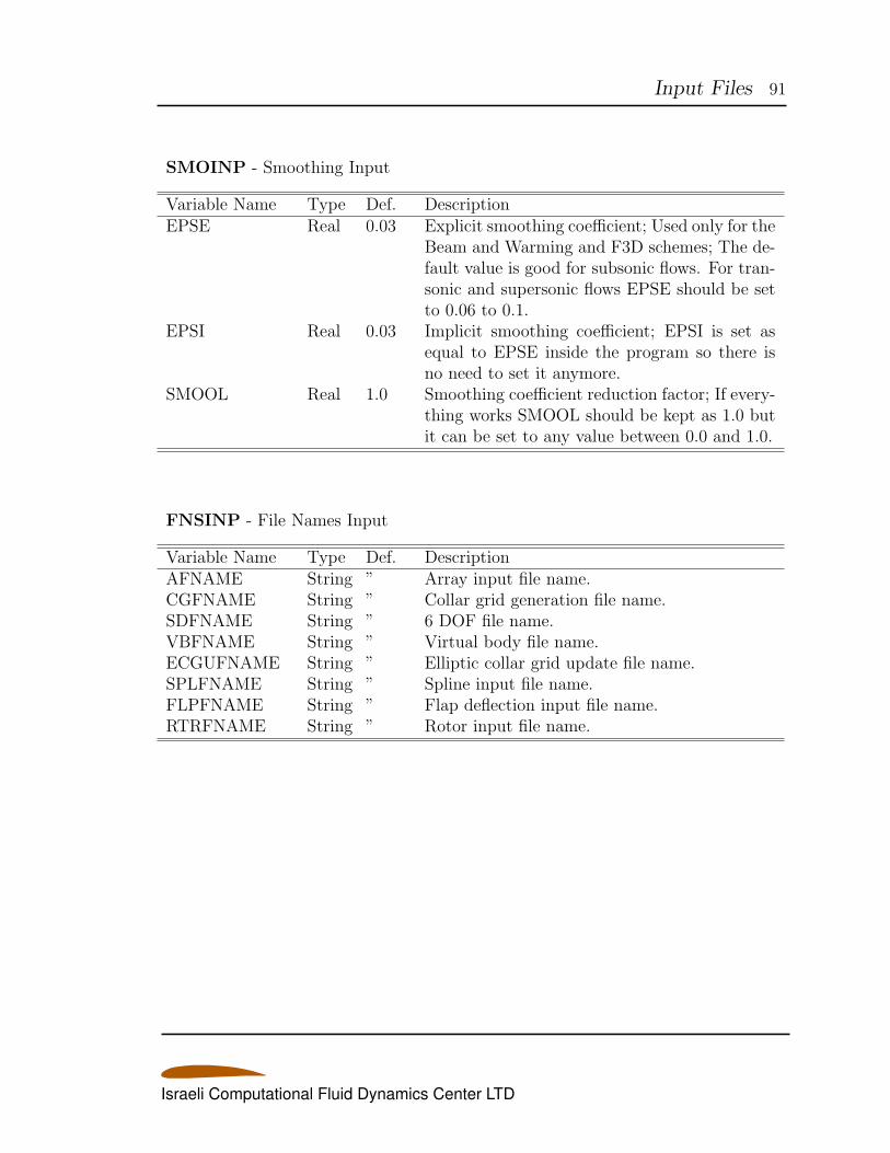
Input Files 91
SMOINP - Smoothing Input
Variable Name Type Def. DescriptionEPSE Real 0.03 Explicit smoothing coefficient; Used only for the
Beam and Warming and F3D schemes; The de-fault value is good for subsonic flows. For tran-sonic and supersonic flows EPSE should be setto 0.06 to 0.1.
EPSI Real 0.03 Implicit smoothing coefficient; EPSI is set asequal to EPSE inside the program so there isno need to set it anymore.
SMOOL Real 1.0 Smoothing coefficient reduction factor; If every-thing works SMOOL should be kept as 1.0 butit can be set to any value between 0.0 and 1.0.
FNSINP - File Names Input
Variable Name Type Def. DescriptionAFNAME String ” Array input file name.CGFNAME String ” Collar grid generation file name.SDFNAME String ” 6 DOF file name.VBFNAME String ” Virtual body file name.ECGUFNAME String ” Elliptic collar grid update file name.SPLFNAME String ” Spline input file name.FLPFNAME String ” Flap deflection input file name.RTRFNAME String ” Rotor input file name.
Israeli Computational Fluid Dynamics Center LTD
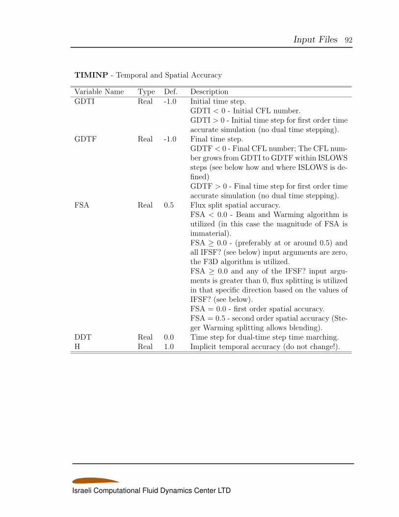
Input Files 92
TIMINP - Temporal and Spatial Accuracy
Variable Name Type Def. DescriptionGDTI Real -1.0 Initial time step.
GDTI < 0 - Initial CFL number.GDTI > 0 - Initial time step for first order timeaccurate simulation (no dual time stepping).
GDTF Real -1.0 Final time step.GDTF < 0 - Final CFL number; The CFL num-ber grows from GDTI to GDTF within ISLOWSsteps (see below how and where ISLOWS is de-fined)GDTF > 0 - Final time step for first order timeaccurate simulation (no dual time stepping).
FSA Real 0.5 Flux split spatial accuracy.FSA < 0.0 - Beam and Warming algorithm isutilized (in this case the magnitude of FSA isimmaterial).FSA ≥ 0.0 - (preferably at or around 0.5) andall IFSF? (see below) input arguments are zero,the F3D algorithm is utilized.FSA ≥ 0.0 and any of the IFSF? input argu-ments is greater than 0, flux splitting is utilizedin that specific direction based on the values ofIFSF? (see below).FSA = 0.0 - first order spatial accuracy.FSA = 0.5 - second order spatial accuracy (Ste-ger Warming splitting allows blending).
DDT Real 0.0 Time step for dual-time step time marching.H Real 1.0 Implicit temporal accuracy (do not change!).
Israeli Computational Fluid Dynamics Center LTD
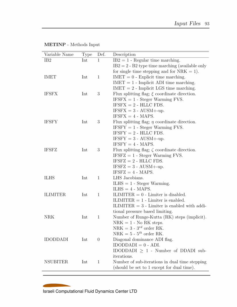
Input Files 93
METINP - Methods Input
Variable Name Type Def. DescriptionIB2 Int 1 IB2 = 1 - Regular time marching.
IB2 = 2 - B2 type time marching (available onlyfor single time stepping and for NRK = 1).
IMET Int 1 IMET = 0 - Explicit time marching.IMET = 1 - Implicit ADI time marching.IMET = 2 - Implicit LGS time marching.
IFSFX Int 3 Flux splitting flag; ξ coordinate direction.IFSFX = 1 - Steger Warming FVS.IFSFX = 2 - HLLC FDS.IFSFX = 3 - AUSM+-up.IFSFX = 4 - MAPS.
IFSFY Int 3 Flux splitting flag; η coordinate direction.IFSFY = 1 - Steger Warming FVS.IFSFY = 2 - HLLC FDS.IFSFY = 3 - AUSM+-up.IFSFY = 4 - MAPS.
IFSFZ Int 3 Flux splitting flag; ζ coordinate direction.IFSFZ = 1 - Steger Warming FVS.IFSFZ = 2 - HLLC FDS.IFSFZ = 3 - AUSM+-up.IFSFZ = 4 - MAPS.
ILHS Int 1 LHS Jacobians.ILHS = 1 - Steger Warming.ILHS = 4 - MAPS.
ILIMITER Int 1 ILIMITER = 0 - Limiter is disabled.ILIMITER = 1 - Limiter is enabled.ILIMITER = 3 - Limiter is enabled with addi-tional pressure based limiting.
NRK Int 1 Number of Runge-Kutta (RK) steps (implicit).NRK = 1 - No RK steps.NRK = 3 - 3rd order RK.NRK = 5 - 5th order RK.
IDODDADI Int 0 Diagonal dominance ADI flag.IDODDADI = 0 - ADI.IDODDADI ≥ 1 - Number of DDADI sub-iterations.
NSUBITER Int 1 Number of sub-iterations in dual time stepping(should be set to 1 except for dual time).
Israeli Computational Fluid Dynamics Center LTD
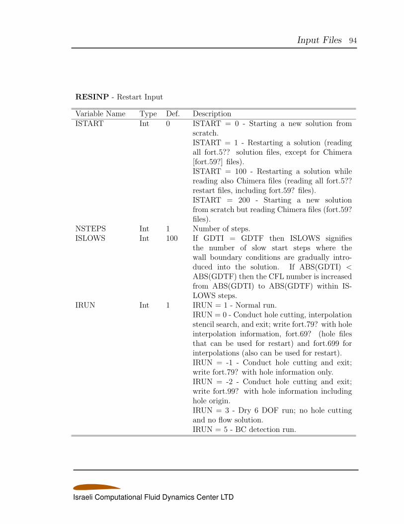
Input Files 94
RESINP - Restart Input
Variable Name Type Def. DescriptionISTART Int 0 ISTART = 0 - Starting a new solution from
scratch.ISTART = 1 - Restarting a solution (readingall fort.5?? solution files, except for Chimera[fort.59?] files).ISTART = 100 - Restarting a solution whilereading also Chimera files (reading all fort.5??restart files, including fort.59? files).ISTART = 200 - Starting a new solutionfrom scratch but reading Chimera files (fort.59?files).
NSTEPS Int 1 Number of steps.ISLOWS Int 100 If GDTI = GDTF then ISLOWS signifies
the number of slow start steps where thewall boundary conditions are gradually intro-duced into the solution. If ABS(GDTI) <ABS(GDTF) then the CFL number is increasedfrom ABS(GDTI) to ABS(GDTF) within IS-LOWS steps.
IRUN Int 1 IRUN = 1 - Normal run.IRUN = 0 - Conduct hole cutting, interpolationstencil search, and exit; write fort.79? with holeinterpolation information, fort.69? (hole filesthat can be used for restart) and fort.699 forinterpolations (also can be used for restart).IRUN = -1 - Conduct hole cutting and exit;write fort.79? with hole information only.IRUN = -2 - Conduct hole cutting and exit;write fort.99? with hole information includinghole origin.IRUN = 3 - Dry 6 DOF run; no hole cuttingand no flow solution.IRUN = 5 - BC detection run.
Israeli Computational Fluid Dynamics Center LTD
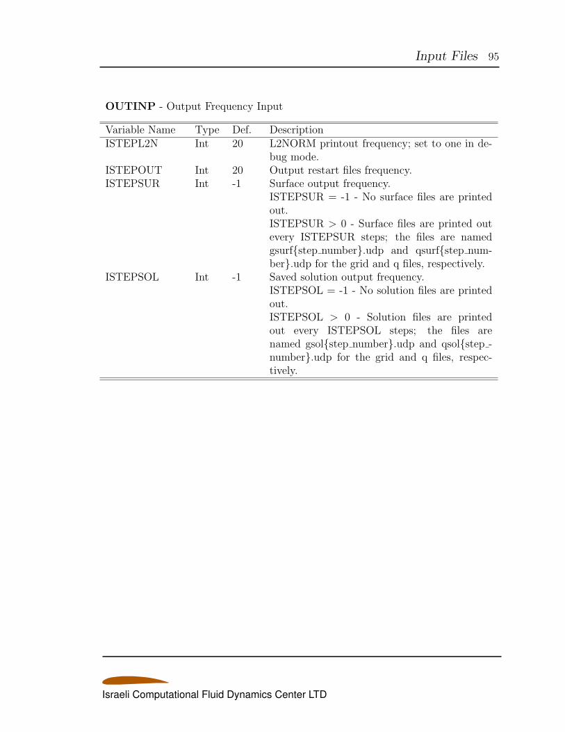
Input Files 95
OUTINP - Output Frequency Input
Variable Name Type Def. DescriptionISTEPL2N Int 20 L2NORM printout frequency; set to one in de-
bug mode.ISTEPOUT Int 20 Output restart files frequency.ISTEPSUR Int -1 Surface output frequency.
ISTEPSUR = -1 - No surface files are printedout.ISTEPSUR > 0 - Surface files are printed outevery ISTEPSUR steps; the files are namedgsurfstep number.udp and qsurfstep num-ber.udp for the grid and q files, respectively.
ISTEPSOL Int -1 Saved solution output frequency.ISTEPSOL = -1 - No solution files are printedout.ISTEPSOL > 0 - Solution files are printedout every ISTEPSOL steps; the files arenamed gsolstep number.udp and qsolstep -number.udp for the grid and q files, respec-tively.
Israeli Computational Fluid Dynamics Center LTD
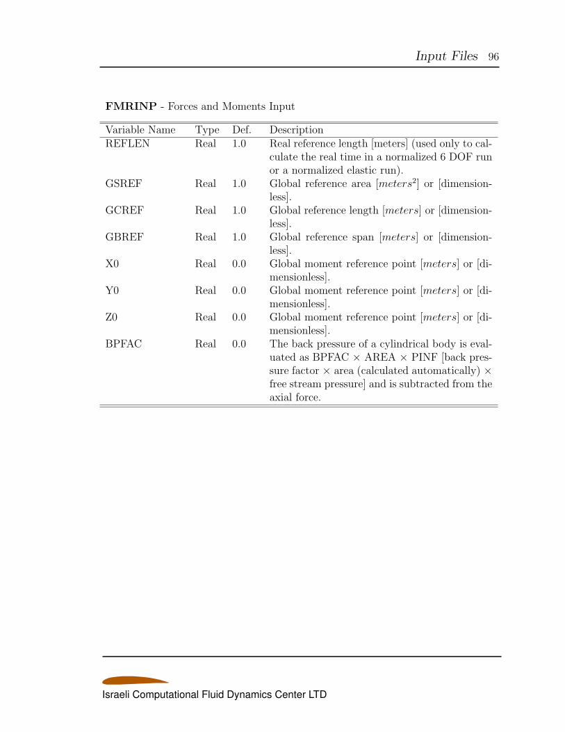
Input Files 96
FMRINP - Forces and Moments Input
Variable Name Type Def. DescriptionREFLEN Real 1.0 Real reference length [meters] (used only to cal-
culate the real time in a normalized 6 DOF runor a normalized elastic run).
GSREF Real 1.0 Global reference area [meters2] or [dimension-less].
GCREF Real 1.0 Global reference length [meters] or [dimension-less].
GBREF Real 1.0 Global reference span [meters] or [dimension-less].
X0 Real 0.0 Global moment reference point [meters] or [di-mensionless].
Y0 Real 0.0 Global moment reference point [meters] or [di-mensionless].
Z0 Real 0.0 Global moment reference point [meters] or [di-mensionless].
BPFAC Real 0.0 The back pressure of a cylindrical body is eval-uated as BPFAC × AREA × PINF [back pres-sure factor × area (calculated automatically) ×free stream pressure] and is subtracted from theaxial force.
Israeli Computational Fluid Dynamics Center LTD
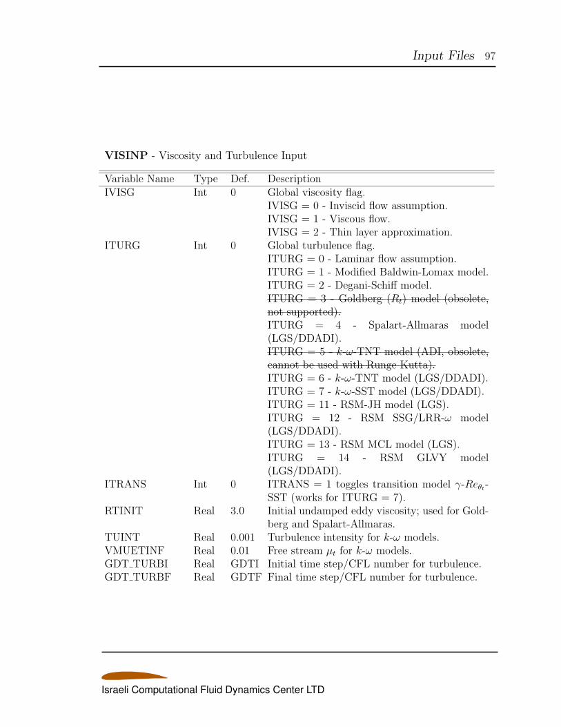
Input Files 97
VISINP - Viscosity and Turbulence Input
Variable Name Type Def. DescriptionIVISG Int 0 Global viscosity flag.
IVISG = 0 - Inviscid flow assumption.IVISG = 1 - Viscous flow.IVISG = 2 - Thin layer approximation.
ITURG Int 0 Global turbulence flag.ITURG = 0 - Laminar flow assumption.ITURG = 1 - Modified Baldwin-Lomax model.ITURG = 2 - Degani-Schiff model.ITURG = 3 - Goldberg (Rt) model (obsolete,not supported).ITURG = 4 - Spalart-Allmaras model(LGS/DDADI).ITURG = 5 - k-ω-TNT model (ADI, obsolete,cannot be used with Runge Kutta).ITURG = 6 - k-ω-TNT model (LGS/DDADI).ITURG = 7 - k-ω-SST model (LGS/DDADI).ITURG = 11 - RSM-JH model (LGS).ITURG = 12 - RSM SSG/LRR-ω model(LGS/DDADI).ITURG = 13 - RSM MCL model (LGS).ITURG = 14 - RSM GLVY model(LGS/DDADI).
ITRANS Int 0 ITRANS = 1 toggles transition model γ-Reθt-SST (works for ITURG = 7).
RTINIT Real 3.0 Initial undamped eddy viscosity; used for Gold-berg and Spalart-Allmaras.
TUINT Real 0.001 Turbulence intensity for k-ω models.VMUETINF Real 0.01 Free stream µt for k-ω models.GDT TURBI Real GDTI Initial time step/CFL number for turbulence.GDT TURBF Real GDTF Final time step/CFL number for turbulence.
Israeli Computational Fluid Dynamics Center LTD
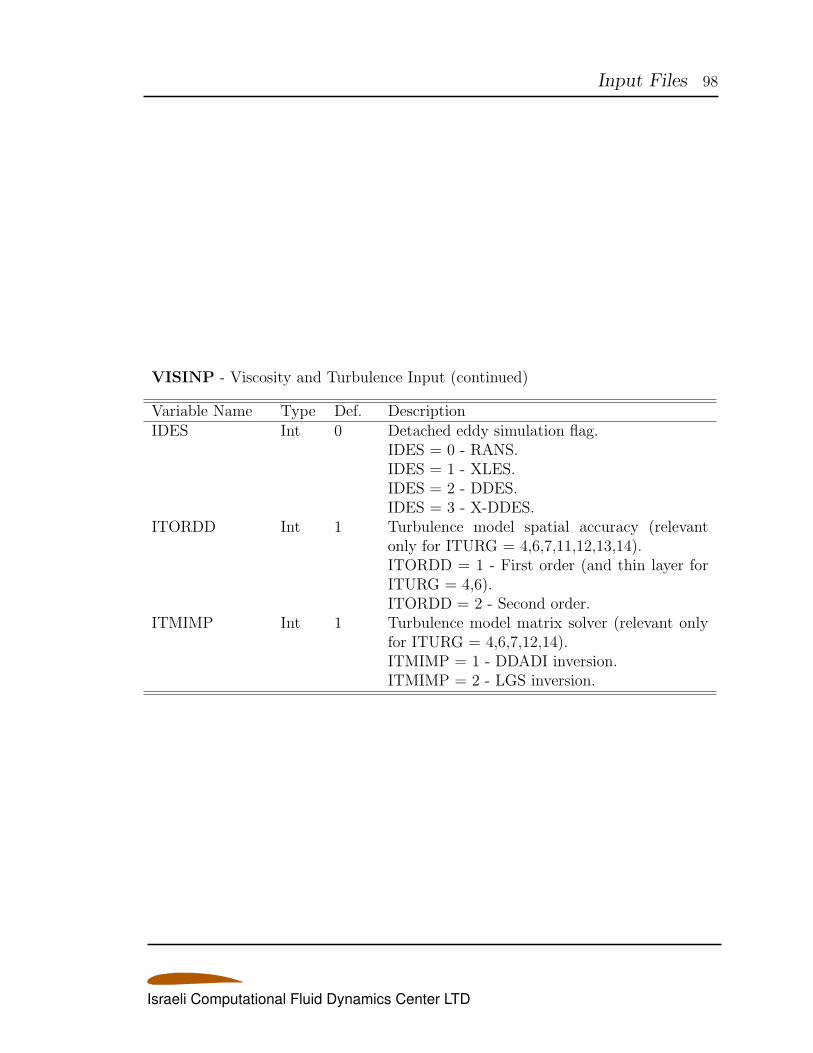
Input Files 98
VISINP - Viscosity and Turbulence Input (continued)
Variable Name Type Def. DescriptionIDES Int 0 Detached eddy simulation flag.
IDES = 0 - RANS.IDES = 1 - XLES.IDES = 2 - DDES.IDES = 3 - X-DDES.
ITORDD Int 1 Turbulence model spatial accuracy (relevantonly for ITURG = 4,6,7,11,12,13,14).ITORDD = 1 - First order (and thin layer forITURG = 4,6).ITORDD = 2 - Second order.
ITMIMP Int 1 Turbulence model matrix solver (relevant onlyfor ITURG = 4,6,7,12,14).ITMIMP = 1 - DDADI inversion.ITMIMP = 2 - LGS inversion.
Israeli Computational Fluid Dynamics Center LTD
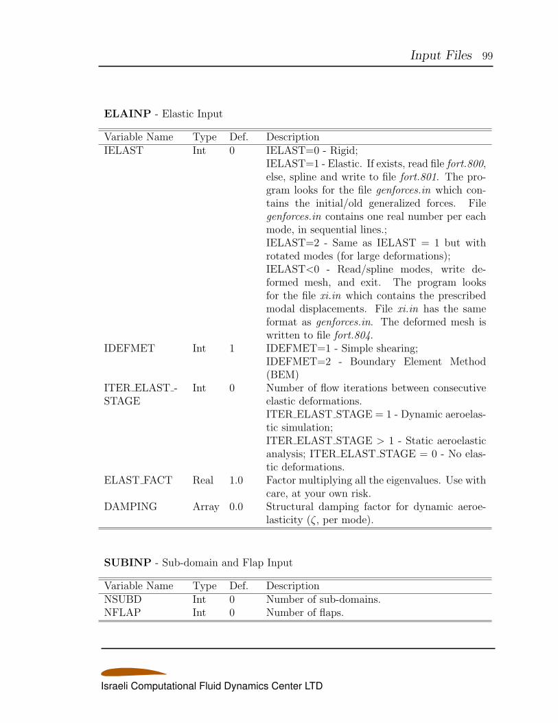
Input Files 99
ELAINP - Elastic Input
Variable Name Type Def. DescriptionIELAST Int 0 IELAST=0 - Rigid;
IELAST=1 - Elastic. If exists, read file fort.800,else, spline and write to file fort.801. The pro-gram looks for the file genforces.in which con-tains the initial/old generalized forces. Filegenforces.in contains one real number per eachmode, in sequential lines.;IELAST=2 - Same as IELAST = 1 but withrotated modes (for large deformations);IELAST<0 - Read/spline modes, write de-formed mesh, and exit. The program looksfor the file xi.in which contains the prescribedmodal displacements. File xi.in has the sameformat as genforces.in. The deformed mesh iswritten to file fort.804.
IDEFMET Int 1 IDEFMET=1 - Simple shearing;IDEFMET=2 - Boundary Element Method(BEM)
ITER ELAST -STAGE
Int 0 Number of flow iterations between consecutiveelastic deformations.ITER ELAST STAGE = 1 - Dynamic aeroelas-tic simulation;ITER ELAST STAGE > 1 - Static aeroelasticanalysis; ITER ELAST STAGE = 0 - No elas-tic deformations.
ELAST FACT Real 1.0 Factor multiplying all the eigenvalues. Use withcare, at your own risk.
DAMPING Array 0.0 Structural damping factor for dynamic aeroe-lasticity (ζ, per mode).
SUBINP - Sub-domain and Flap Input
Variable Name Type Def. DescriptionNSUBD Int 0 Number of sub-domains.NFLAP Int 0 Number of flaps.
Israeli Computational Fluid Dynamics Center LTD
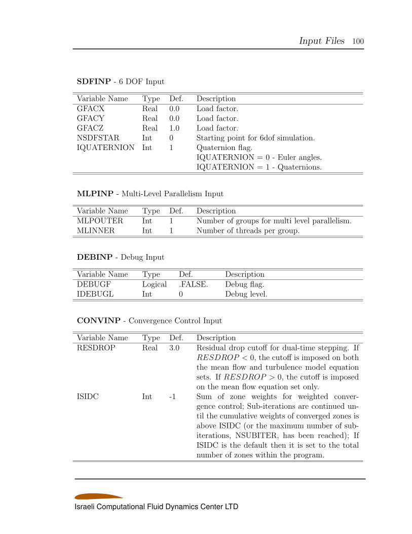
Input Files 100
SDFINP - 6 DOF Input
Variable Name Type Def. DescriptionGFACX Real 0.0 Load factor.GFACY Real 0.0 Load factor.GFACZ Real 1.0 Load factor.NSDFSTAR Int 0 Starting point for 6dof simulation.IQUATERNION Int 1 Quaternion flag.
IQUATERNION = 0 - Euler angles.IQUATERNION = 1 - Quaternions.
MLPINP - Multi-Level Parallelism Input
Variable Name Type Def. DescriptionMLPOUTER Int 1 Number of groups for multi level parallelism.MLINNER Int 1 Number of threads per group.
DEBINP - Debug Input
Variable Name Type Def. DescriptionDEBUGF Logical .FALSE. Debug flag.IDEBUGL Int 0 Debug level.
CONVINP - Convergence Control Input
Variable Name Type Def. DescriptionRESDROP Real 3.0 Residual drop cutoff for dual-time stepping. If
RESDROP < 0, the cutoff is imposed on boththe mean flow and turbulence model equationsets. If RESDROP > 0, the cutoff is imposedon the mean flow equation set only.
ISIDC Int -1 Sum of zone weights for weighted conver-gence control; Sub-iterations are continued un-til the cumulative weights of converged zones isabove ISIDC (or the maximum number of sub-iterations, NSUBITER, has been reached); IfISIDC is the default then it is set to the totalnumber of zones within the program.
Israeli Computational Fluid Dynamics Center LTD
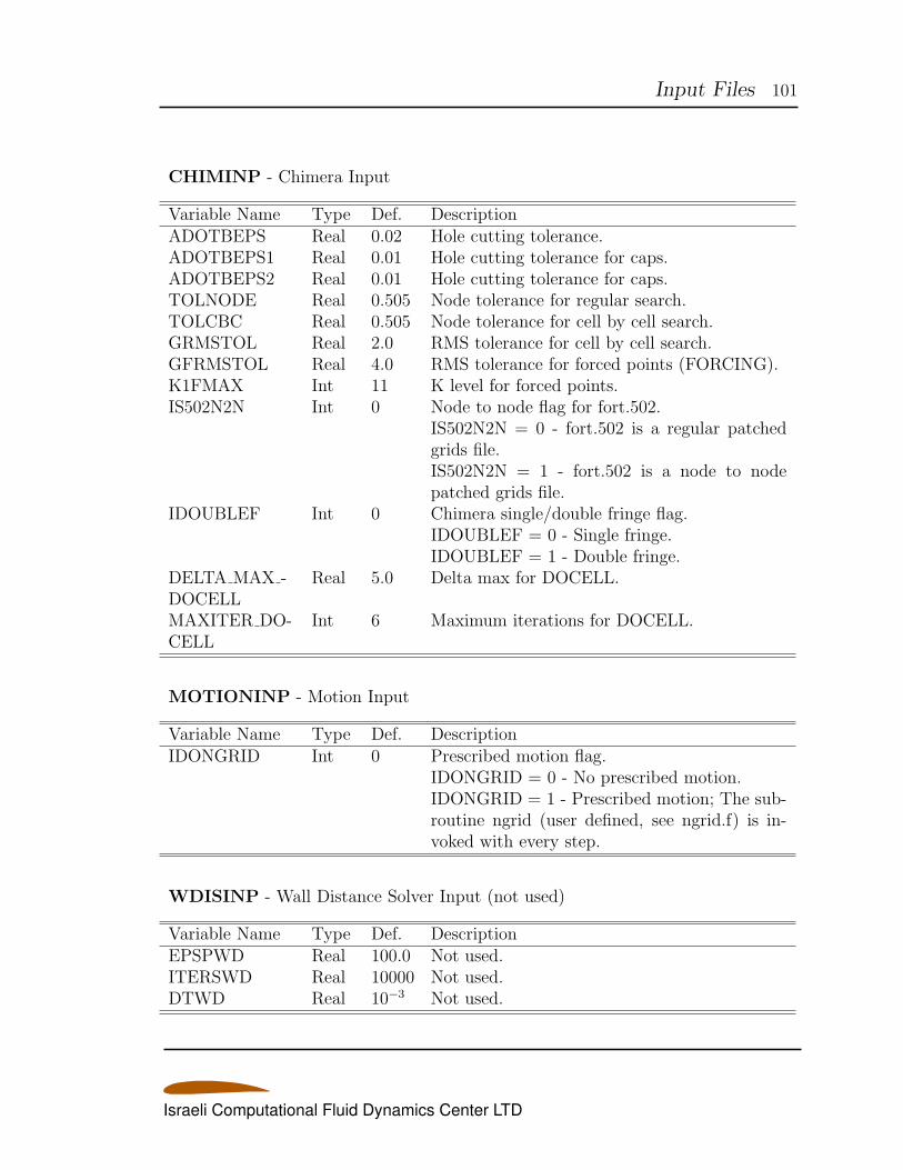
Input Files 101
CHIMINP - Chimera Input
Variable Name Type Def. DescriptionADOTBEPS Real 0.02 Hole cutting tolerance.ADOTBEPS1 Real 0.01 Hole cutting tolerance for caps.ADOTBEPS2 Real 0.01 Hole cutting tolerance for caps.TOLNODE Real 0.505 Node tolerance for regular search.TOLCBC Real 0.505 Node tolerance for cell by cell search.GRMSTOL Real 2.0 RMS tolerance for cell by cell search.GFRMSTOL Real 4.0 RMS tolerance for forced points (FORCING).K1FMAX Int 11 K level for forced points.IS502N2N Int 0 Node to node flag for fort.502.
IS502N2N = 0 - fort.502 is a regular patchedgrids file.IS502N2N = 1 - fort.502 is a node to nodepatched grids file.
IDOUBLEF Int 0 Chimera single/double fringe flag.IDOUBLEF = 0 - Single fringe.IDOUBLEF = 1 - Double fringe.
DELTA MAX -DOCELL
Real 5.0 Delta max for DOCELL.
MAXITER DO-CELL
Int 6 Maximum iterations for DOCELL.
MOTIONINP - Motion Input
Variable Name Type Def. DescriptionIDONGRID Int 0 Prescribed motion flag.
IDONGRID = 0 - No prescribed motion.IDONGRID = 1 - Prescribed motion; The sub-routine ngrid (user defined, see ngrid.f) is in-voked with every step.
WDISINP - Wall Distance Solver Input (not used)
Variable Name Type Def. DescriptionEPSPWD Real 100.0 Not used.ITERSWD Real 10000 Not used.DTWD Real 10−3 Not used.
Israeli Computational Fluid Dynamics Center LTD
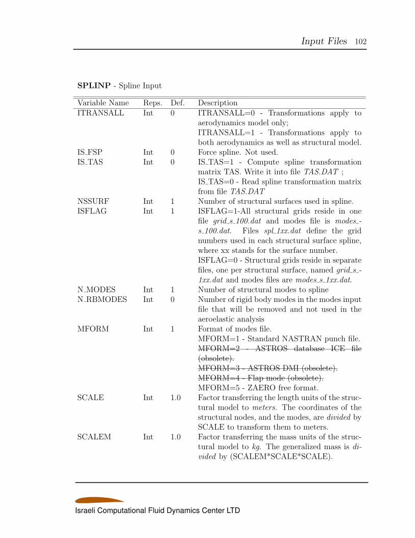
Input Files 102
SPLINP - Spline Input
Variable Name Reps. Def. DescriptionITRANSALL Int 0 ITRANSALL=0 - Transformations apply to
aerodynamics model only;ITRANSALL=1 - Transformations apply toboth aerodynamics as well as structural model.
IS FSP Int 0 Force spline. Not used.IS TAS Int 0 IS TAS=1 - Compute spline transformation
matrix TAS. Write it into file TAS.DAT ;IS TAS=0 - Read spline transformation matrixfrom file TAS.DAT
NSSURF Int 1 Number of structural surfaces used in spline.ISFLAG Int 1 ISFLAG=1-All structural grids reside in one
file grid s 100.dat and modes file is modes -s 100.dat. Files spl 1xx.dat define the gridnumbers used in each structural surface spline,where xx stands for the surface number.ISFLAG=0 - Structural grids reside in separatefiles, one per structural surface, named grid s -1xx.dat and modes files are modes s 1xx.dat.
N MODES Int 1 Number of structural modes to splineN RBMODES Int 0 Number of rigid body modes in the modes input
file that will be removed and not used in theaeroelastic analysis
MFORM Int 1 Format of modes file.MFORM=1 - Standard NASTRAN punch file.MFORM=2 - ASTROS database ICE file(obsolete).MFORM=3 - ASTROS DMI (obsolete).MFORM=4 - Flap mode (obsolete).MFORM=5 - ZAERO free format.
SCALE Int 1.0 Factor transferring the length units of the struc-tural model to meters. The coordinates of thestructural nodes, and the modes, are divided bySCALE to transform them to meters.
SCALEM Int 1.0 Factor transferring the mass units of the struc-tural model to kg. The generalized mass is di-vided by (SCALEM*SCALE*SCALE).
Israeli Computational Fluid Dynamics Center LTD
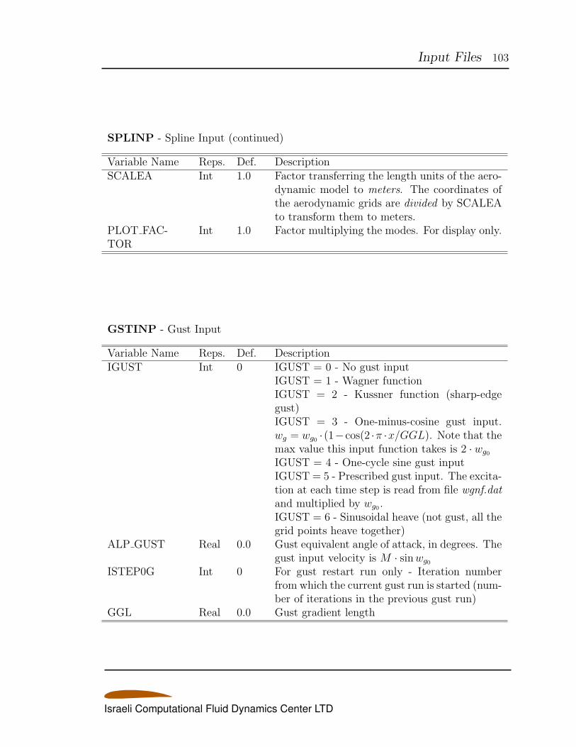
Input Files 103
SPLINP - Spline Input (continued)
Variable Name Reps. Def. DescriptionSCALEA Int 1.0 Factor transferring the length units of the aero-
dynamic model to meters. The coordinates ofthe aerodynamic grids are divided by SCALEAto transform them to meters.
PLOT FAC-TOR
Int 1.0 Factor multiplying the modes. For display only.
GSTINP - Gust Input
Variable Name Reps. Def. DescriptionIGUST Int 0 IGUST = 0 - No gust input
IGUST = 1 - Wagner functionIGUST = 2 - Kussner function (sharp-edgegust)IGUST = 3 - One-minus-cosine gust input.wg = wg0 · (1−cos(2 ·π ·x/GGL). Note that themax value this input function takes is 2 · wg0
IGUST = 4 - One-cycle sine gust inputIGUST = 5 - Prescribed gust input. The excita-tion at each time step is read from file wgnf.datand multiplied by wg0 .IGUST = 6 - Sinusoidal heave (not gust, all thegrid points heave together)
ALP GUST Real 0.0 Gust equivalent angle of attack, in degrees. Thegust input velocity is M · sinwg0
ISTEP0G Int 0 For gust restart run only - Iteration numberfrom which the current gust run is started (num-ber of iterations in the previous gust run)
GGL Real 0.0 Gust gradient length
Israeli Computational Fluid Dynamics Center LTD
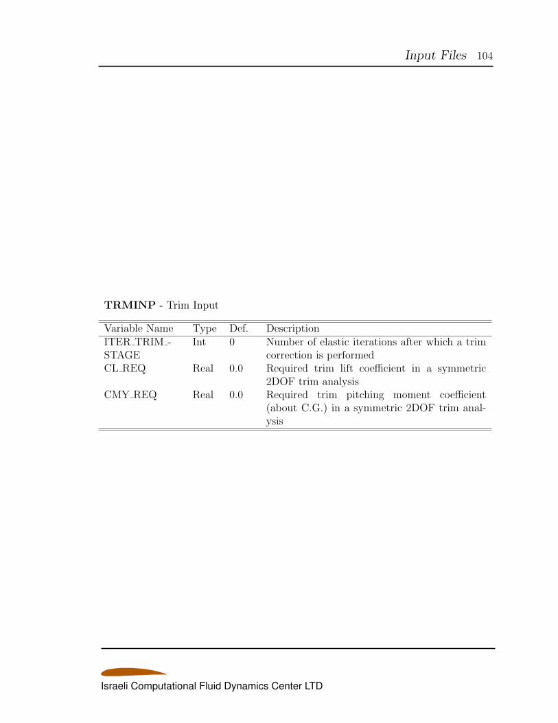
Input Files 104
TRMINP - Trim Input
Variable Name Type Def. DescriptionITER TRIM -STAGE
Int 0 Number of elastic iterations after which a trimcorrection is performed
CL REQ Real 0.0 Required trim lift coefficient in a symmetric2DOF trim analysis
CMY REQ Real 0.0 Required trim pitching moment coefficient(about C.G.) in a symmetric 2DOF trim anal-ysis
Israeli Computational Fluid Dynamics Center LTD
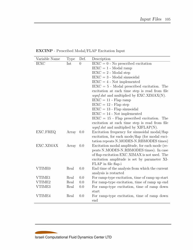
Input Files 105
EXCINP - Prescribed Modal/FLAP Excitation Input
Variable Name Type Def. DescriptionIEXC Int 0 IEXC = 0 - No prescribed excitation
IEXC = 1 - Modal rampIEXC = 2 - Modal stepIEXC = 3 - Modal sinusoidalIEXC = 4 - Not implementedIEXC = 5 - Modal prescribed excitation. Theexcitation at each time step is read from filewgnf.dat and multiplied by EXC XIMAX(N).IEXC = 11 - Flap rampIEXC = 12 - Flap stepIEXC = 13 - Flap sinusoidalIEXC = 14 - Not implementedIEXC = 15 - Flap prescribed excitation. Theexcitation at each time step is read from filewgnf.dat and multiplied by XIFLAP(N).
EXC FREQ Array 0.0 Excitation frequency for sinusoidal modal/flapexcitation, for each mode/flap (for modal exci-tation repeats N MODES-N RBMODES times)
EXC XIMAX Array 0.0 Excitation modal amplitude, for each mode (re-peats N MODES-N RBMODES times). In caseof flap excitation EXC XIMAX is not used. Theexcitation amplitude is set by parameter XI-FLAP in file flap.i
VTIME0 Real 0.0 End time of the analysis from which the currentanalysis is restarted
VTIME1 Real 0.0 For ramp-type excitation, time of ramp up startVTIME2 Real 0.0 For ramp-type excitation, time of ramp up endVTIME3 Real 0.0 For ramp-type excitation, time of ramp down
startVTIME4 Real 0.0 For ramp-type excitation, time of ramp down
end
Israeli Computational Fluid Dynamics Center LTD
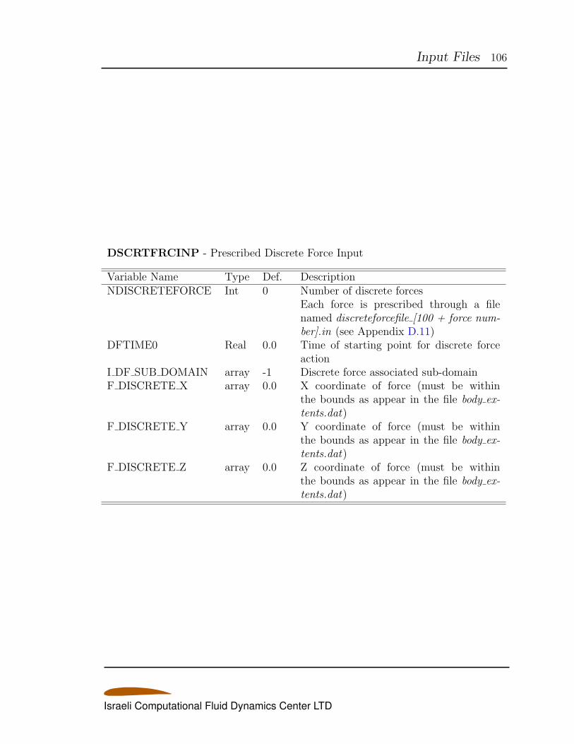
Input Files 106
DSCRTFRCINP - Prescribed Discrete Force Input
Variable Name Type Def. DescriptionNDISCRETEFORCE Int 0 Number of discrete forces
Each force is prescribed through a filenamed discreteforcefile [100 + force num-ber].in (see Appendix D.11)
DFTIME0 Real 0.0 Time of starting point for discrete forceaction
I DF SUB DOMAIN array -1 Discrete force associated sub-domainF DISCRETE X array 0.0 X coordinate of force (must be within
the bounds as appear in the file body ex-tents.dat)
F DISCRETE Y array 0.0 Y coordinate of force (must be withinthe bounds as appear in the file body ex-tents.dat)
F DISCRETE Z array 0.0 Z coordinate of force (must be withinthe bounds as appear in the file body ex-tents.dat)
Israeli Computational Fluid Dynamics Center LTD
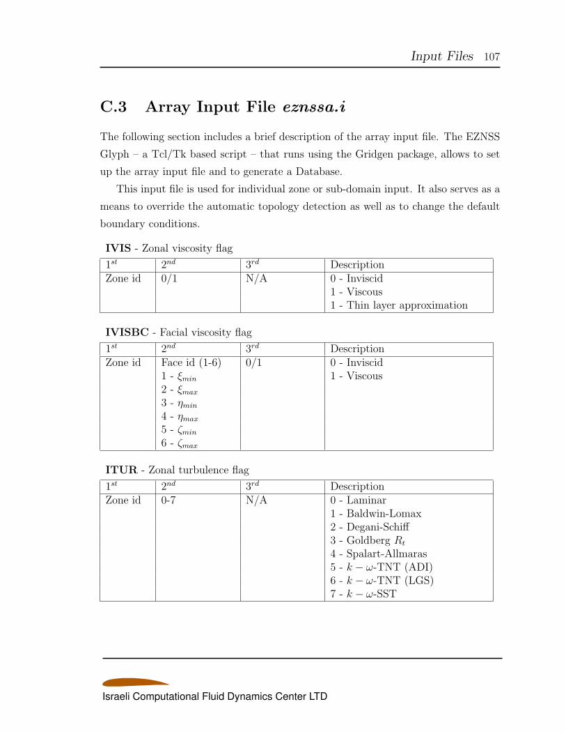
Input Files 107
C.3 Array Input File eznssa.i
The following section includes a brief description of the array input file. The EZNSS
Glyph – a Tcl/Tk based script – that runs using the Gridgen package, allows to set
up the array input file and to generate a Database.
This input file is used for individual zone or sub-domain input. It also serves as a
means to override the automatic topology detection as well as to change the default
boundary conditions.
IVIS - Zonal viscosity flag
1st 2nd 3rd DescriptionZone id 0/1 N/A 0 - Inviscid
1 - Viscous1 - Thin layer approximation
IVISBC - Facial viscosity flag
1st 2nd 3rd DescriptionZone id Face id (1-6) 0/1 0 - Inviscid
1 - ξmin 1 - Viscous2 - ξmax
3 - ηmin
4 - ηmax
5 - ζmin
6 - ζmax
ITUR - Zonal turbulence flag
1st 2nd 3rd DescriptionZone id 0-7 N/A 0 - Laminar
1 - Baldwin-Lomax2 - Degani-Schiff3 - Goldberg Rt
4 - Spalart-Allmaras5 - k − ω-TNT (ADI)6 - k − ω-TNT (LGS)7 - k − ω-SST
Israeli Computational Fluid Dynamics Center LTD
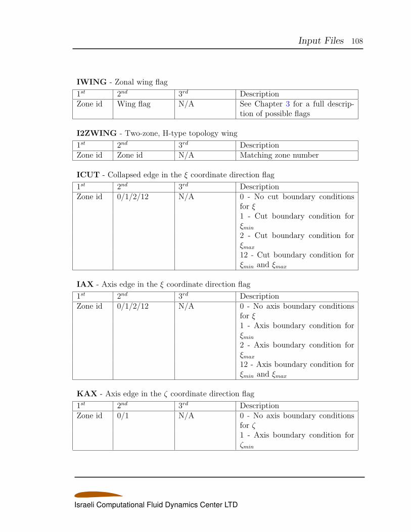
Input Files 108
IWING - Zonal wing flag
1st 2nd 3rd DescriptionZone id Wing flag N/A See Chapter 3 for a full descrip-
tion of possible flags
I2ZWING - Two-zone, H-type topology wing
1st 2nd 3rd DescriptionZone id Zone id N/A Matching zone number
ICUT - Collapsed edge in the ξ coordinate direction flag
1st 2nd 3rd DescriptionZone id 0/1/2/12 N/A 0 - No cut boundary conditions
for ξ1 - Cut boundary condition forξmin
2 - Cut boundary condition forξmax
12 - Cut boundary condition forξmin and ξmax
IAX - Axis edge in the ξ coordinate direction flag
1st 2nd 3rd DescriptionZone id 0/1/2/12 N/A 0 - No axis boundary conditions
for ξ1 - Axis boundary condition forξmin
2 - Axis boundary condition forξmax
12 - Axis boundary condition forξmin and ξmax
KAX - Axis edge in the ζ coordinate direction flag
1st 2nd 3rd DescriptionZone id 0/1 N/A 0 - No axis boundary conditions
for ζ1 - Axis boundary condition forζmin
Israeli Computational Fluid Dynamics Center LTD
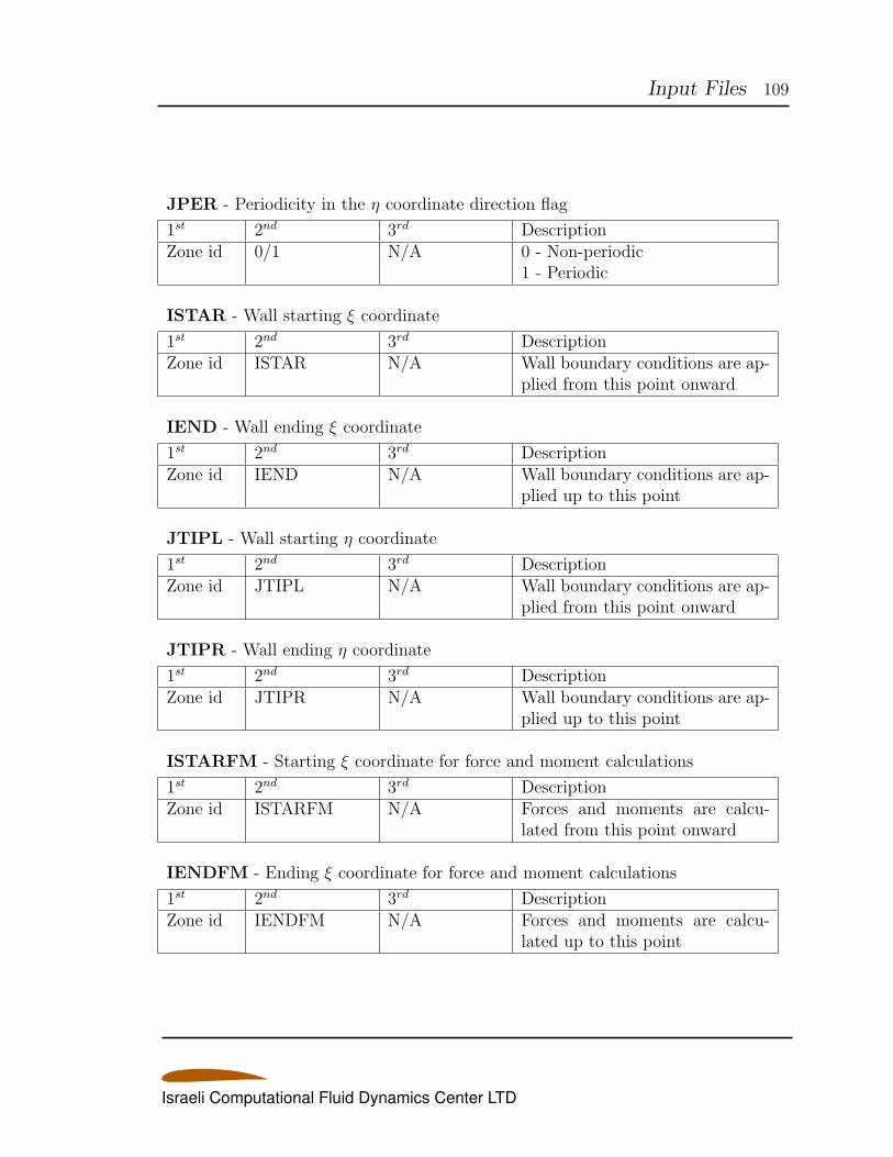
Input Files 109
JPER - Periodicity in the η coordinate direction flag
1st 2nd 3rd DescriptionZone id 0/1 N/A 0 - Non-periodic
1 - Periodic
ISTAR - Wall starting ξ coordinate
1st 2nd 3rd DescriptionZone id ISTAR N/A Wall boundary conditions are ap-
plied from this point onward
IEND - Wall ending ξ coordinate
1st 2nd 3rd DescriptionZone id IEND N/A Wall boundary conditions are ap-
plied up to this point
JTIPL - Wall starting η coordinate
1st 2nd 3rd DescriptionZone id JTIPL N/A Wall boundary conditions are ap-
plied from this point onward
JTIPR - Wall ending η coordinate
1st 2nd 3rd DescriptionZone id JTIPR N/A Wall boundary conditions are ap-
plied up to this point
ISTARFM - Starting ξ coordinate for force and moment calculations
1st 2nd 3rd DescriptionZone id ISTARFM N/A Forces and moments are calcu-
lated from this point onward
IENDFM - Ending ξ coordinate for force and moment calculations
1st 2nd 3rd DescriptionZone id IENDFM N/A Forces and moments are calcu-
lated up to this point
Israeli Computational Fluid Dynamics Center LTD
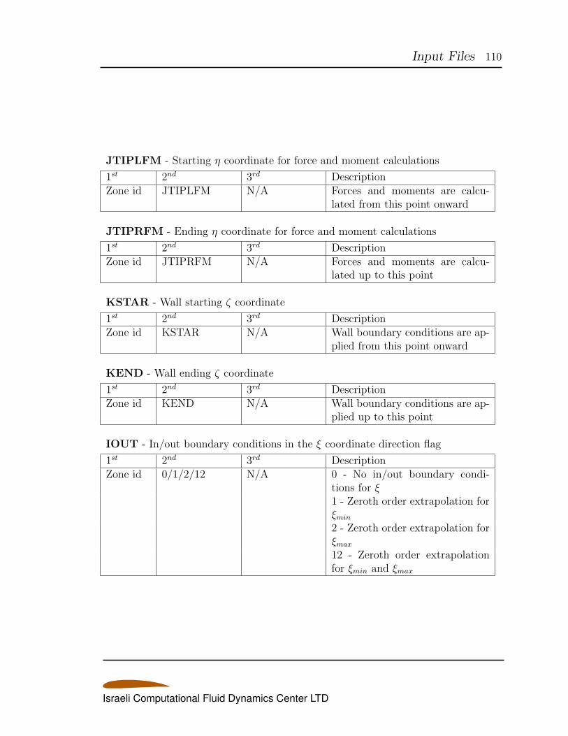
Input Files 110
JTIPLFM - Starting η coordinate for force and moment calculations
1st 2nd 3rd DescriptionZone id JTIPLFM N/A Forces and moments are calcu-
lated from this point onward
JTIPRFM - Ending η coordinate for force and moment calculations
1st 2nd 3rd DescriptionZone id JTIPRFM N/A Forces and moments are calcu-
lated up to this point
KSTAR - Wall starting ζ coordinate
1st 2nd 3rd DescriptionZone id KSTAR N/A Wall boundary conditions are ap-
plied from this point onward
KEND - Wall ending ζ coordinate
1st 2nd 3rd DescriptionZone id KEND N/A Wall boundary conditions are ap-
plied up to this point
IOUT - In/out boundary conditions in the ξ coordinate direction flag
1st 2nd 3rd DescriptionZone id 0/1/2/12 N/A 0 - No in/out boundary condi-
tions for ξ1 - Zeroth order extrapolation forξmin
2 - Zeroth order extrapolation forξmax
12 - Zeroth order extrapolationfor ξmin and ξmax
Israeli Computational Fluid Dynamics Center LTD
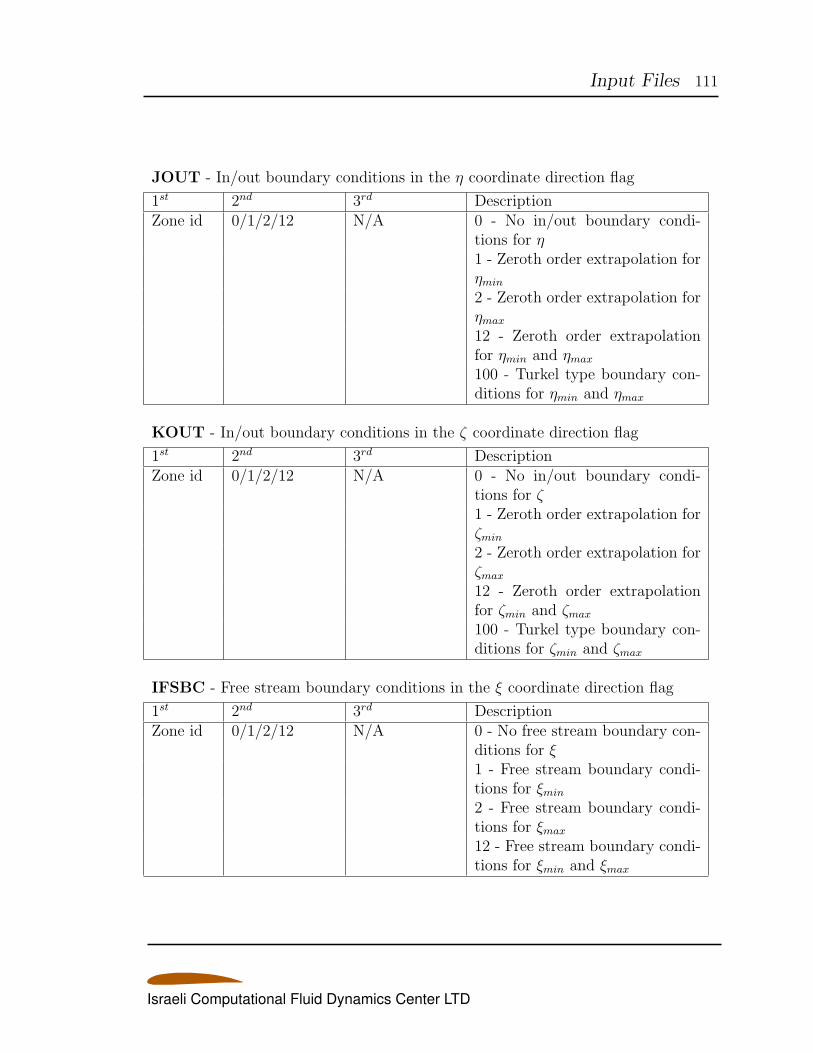
Input Files 111
JOUT - In/out boundary conditions in the η coordinate direction flag
1st 2nd 3rd DescriptionZone id 0/1/2/12 N/A 0 - No in/out boundary condi-
tions for η1 - Zeroth order extrapolation forηmin
2 - Zeroth order extrapolation forηmax
12 - Zeroth order extrapolationfor ηmin and ηmax
100 - Turkel type boundary con-ditions for ηmin and ηmax
KOUT - In/out boundary conditions in the ζ coordinate direction flag
1st 2nd 3rd DescriptionZone id 0/1/2/12 N/A 0 - No in/out boundary condi-
tions for ζ1 - Zeroth order extrapolation forζmin
2 - Zeroth order extrapolation forζmax
12 - Zeroth order extrapolationfor ζmin and ζmax
100 - Turkel type boundary con-ditions for ζmin and ζmax
IFSBC - Free stream boundary conditions in the ξ coordinate direction flag
1st 2nd 3rd DescriptionZone id 0/1/2/12 N/A 0 - No free stream boundary con-
ditions for ξ1 - Free stream boundary condi-tions for ξmin
2 - Free stream boundary condi-tions for ξmax
12 - Free stream boundary condi-tions for ξmin and ξmax
Israeli Computational Fluid Dynamics Center LTD
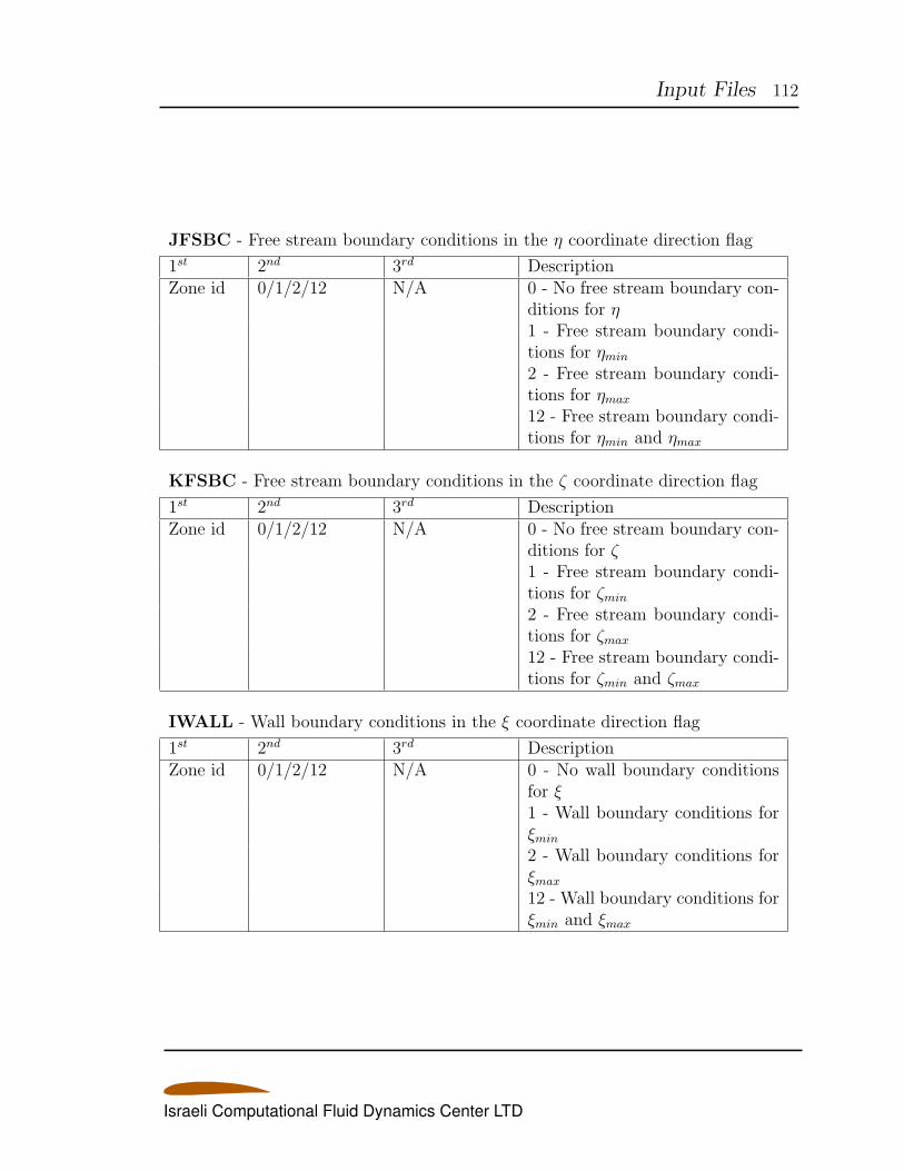
Input Files 112
JFSBC - Free stream boundary conditions in the η coordinate direction flag
1st 2nd 3rd DescriptionZone id 0/1/2/12 N/A 0 - No free stream boundary con-
ditions for η1 - Free stream boundary condi-tions for ηmin
2 - Free stream boundary condi-tions for ηmax
12 - Free stream boundary condi-tions for ηmin and ηmax
KFSBC - Free stream boundary conditions in the ζ coordinate direction flag
1st 2nd 3rd DescriptionZone id 0/1/2/12 N/A 0 - No free stream boundary con-
ditions for ζ1 - Free stream boundary condi-tions for ζmin
2 - Free stream boundary condi-tions for ζmax
12 - Free stream boundary condi-tions for ζmin and ζmax
IWALL - Wall boundary conditions in the ξ coordinate direction flag
1st 2nd 3rd DescriptionZone id 0/1/2/12 N/A 0 - No wall boundary conditions
for ξ1 - Wall boundary conditions forξmin
2 - Wall boundary conditions forξmax
12 - Wall boundary conditions forξmin and ξmax
Israeli Computational Fluid Dynamics Center LTD
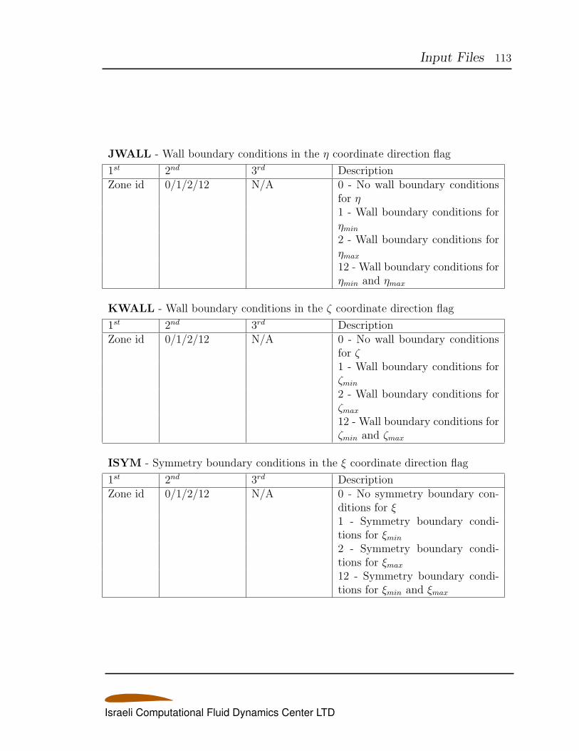
Input Files 113
JWALL - Wall boundary conditions in the η coordinate direction flag
1st 2nd 3rd DescriptionZone id 0/1/2/12 N/A 0 - No wall boundary conditions
for η1 - Wall boundary conditions forηmin
2 - Wall boundary conditions forηmax
12 - Wall boundary conditions forηmin and ηmax
KWALL - Wall boundary conditions in the ζ coordinate direction flag
1st 2nd 3rd DescriptionZone id 0/1/2/12 N/A 0 - No wall boundary conditions
for ζ1 - Wall boundary conditions forζmin
2 - Wall boundary conditions forζmax
12 - Wall boundary conditions forζmin and ζmax
ISYM - Symmetry boundary conditions in the ξ coordinate direction flag
1st 2nd 3rd DescriptionZone id 0/1/2/12 N/A 0 - No symmetry boundary con-
ditions for ξ1 - Symmetry boundary condi-tions for ξmin
2 - Symmetry boundary condi-tions for ξmax
12 - Symmetry boundary condi-tions for ξmin and ξmax
Israeli Computational Fluid Dynamics Center LTD
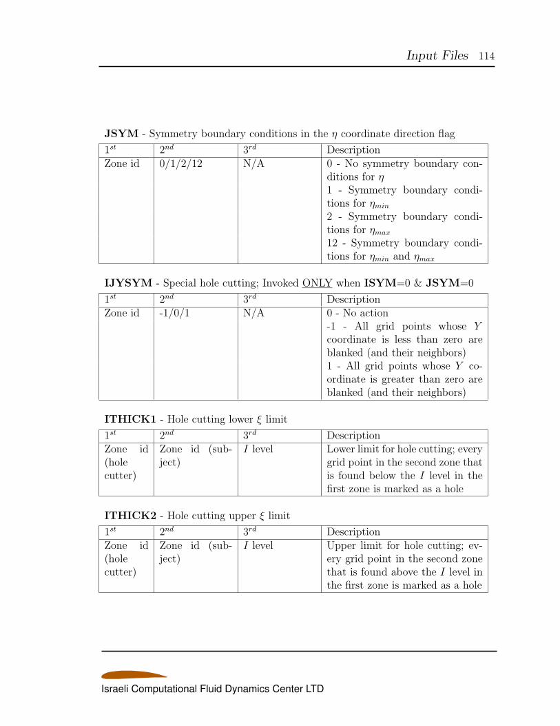
Input Files 114
JSYM - Symmetry boundary conditions in the η coordinate direction flag
1st 2nd 3rd DescriptionZone id 0/1/2/12 N/A 0 - No symmetry boundary con-
ditions for η1 - Symmetry boundary condi-tions for ηmin
2 - Symmetry boundary condi-tions for ηmax
12 - Symmetry boundary condi-tions for ηmin and ηmax
IJYSYM - Special hole cutting; Invoked ONLY when ISYM=0 & JSYM=0
1st 2nd 3rd DescriptionZone id -1/0/1 N/A 0 - No action
-1 - All grid points whose Ycoordinate is less than zero areblanked (and their neighbors)1 - All grid points whose Y co-ordinate is greater than zero areblanked (and their neighbors)
ITHICK1 - Hole cutting lower ξ limit
1st 2nd 3rd DescriptionZone id(holecutter)
Zone id (sub-ject)
I level Lower limit for hole cutting; everygrid point in the second zone thatis found below the I level in thefirst zone is marked as a hole
ITHICK2 - Hole cutting upper ξ limit
1st 2nd 3rd DescriptionZone id(holecutter)
Zone id (sub-ject)
I level Upper limit for hole cutting; ev-ery grid point in the second zonethat is found above the I level inthe first zone is marked as a hole
Israeli Computational Fluid Dynamics Center LTD
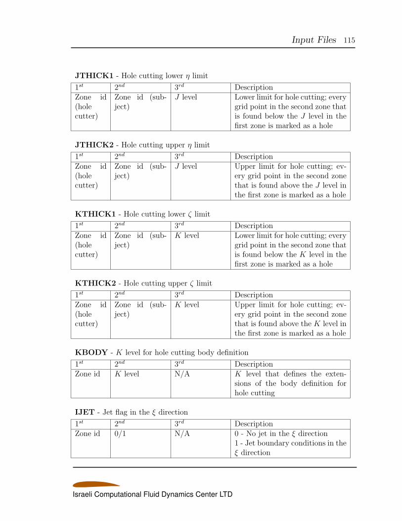
Input Files 115
JTHICK1 - Hole cutting lower η limit
1st 2nd 3rd DescriptionZone id(holecutter)
Zone id (sub-ject)
J level Lower limit for hole cutting; everygrid point in the second zone thatis found below the J level in thefirst zone is marked as a hole
JTHICK2 - Hole cutting upper η limit
1st 2nd 3rd DescriptionZone id(holecutter)
Zone id (sub-ject)
J level Upper limit for hole cutting; ev-ery grid point in the second zonethat is found above the J level inthe first zone is marked as a hole
KTHICK1 - Hole cutting lower ζ limit
1st 2nd 3rd DescriptionZone id(holecutter)
Zone id (sub-ject)
K level Lower limit for hole cutting; everygrid point in the second zone thatis found below the K level in thefirst zone is marked as a hole
KTHICK2 - Hole cutting upper ζ limit
1st 2nd 3rd DescriptionZone id(holecutter)
Zone id (sub-ject)
K level Upper limit for hole cutting; ev-ery grid point in the second zonethat is found above the K level inthe first zone is marked as a hole
KBODY - K level for hole cutting body definition
1st 2nd 3rd DescriptionZone id K level N/A K level that defines the exten-
sions of the body definition forhole cutting
IJET - Jet flag in the ξ direction
1st 2nd 3rd DescriptionZone id 0/1 N/A 0 - No jet in the ξ direction
1 - Jet boundary conditions in theξ direction
Israeli Computational Fluid Dynamics Center LTD
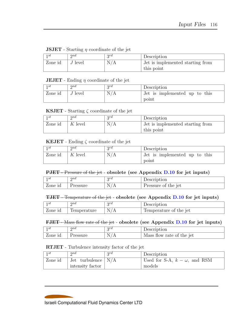
Input Files 116
JSJET - Starting η coordinate of the jet
1st 2nd 3rd DescriptionZone id J level N/A Jet is implemented starting from
this point
JEJET - Ending η coordinate of the jet
1st 2nd 3rd DescriptionZone id J level N/A Jet is implemented up to this
point
KSJET - Starting ζ coordinate of the jet
1st 2nd 3rd DescriptionZone id K level N/A Jet is implemented starting from
this point
KEJET - Ending ζ coordinate of the jet
1st 2nd 3rd DescriptionZone id K level N/A Jet is implemented up to this
point
PJET - Pressure of the jet - obsolete (see Appendix D.10 for jet inputs)
1st 2nd 3rd DescriptionZone id Pressure N/A Pressure of the jet
TJET - Temperature of the jet - obsolete (see Appendix D.10 for jet inputs)
1st 2nd 3rd DescriptionZone id Temperature N/A Temperature of the jet
FJET - Mass flow rate of the jet - obsolete (see Appendix D.10 for jet inputs)
1st 2nd 3rd DescriptionZone id Pressure N/A Mass flow rate of the jet
RTJET - Turbulence intensity factor of the jet
1st 2nd 3rd DescriptionZone id Jet turbulence
intensity factorN/A Used for S-A, k − ω, and RSM
models
Israeli Computational Fluid Dynamics Center LTD
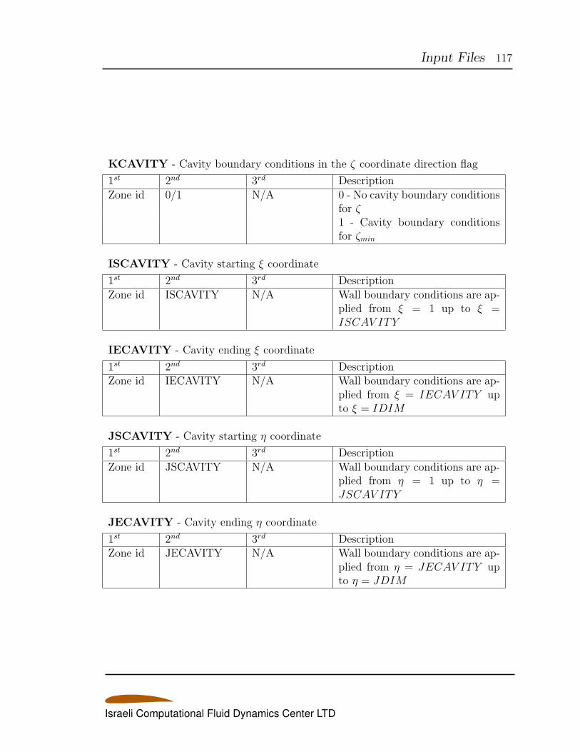
Input Files 117
KCAVITY - Cavity boundary conditions in the ζ coordinate direction flag
1st 2nd 3rd DescriptionZone id 0/1 N/A 0 - No cavity boundary conditions
for ζ1 - Cavity boundary conditionsfor ζmin
ISCAVITY - Cavity starting ξ coordinate
1st 2nd 3rd DescriptionZone id ISCAVITY N/A Wall boundary conditions are ap-
plied from ξ = 1 up to ξ =ISCAV ITY
IECAVITY - Cavity ending ξ coordinate
1st 2nd 3rd DescriptionZone id IECAVITY N/A Wall boundary conditions are ap-
plied from ξ = IECAV ITY upto ξ = IDIM
JSCAVITY - Cavity starting η coordinate
1st 2nd 3rd DescriptionZone id JSCAVITY N/A Wall boundary conditions are ap-
plied from η = 1 up to η =JSCAV ITY
JECAVITY - Cavity ending η coordinate
1st 2nd 3rd DescriptionZone id JECAVITY N/A Wall boundary conditions are ap-
plied from η = JECAV ITY upto η = JDIM
Israeli Computational Fluid Dynamics Center LTD
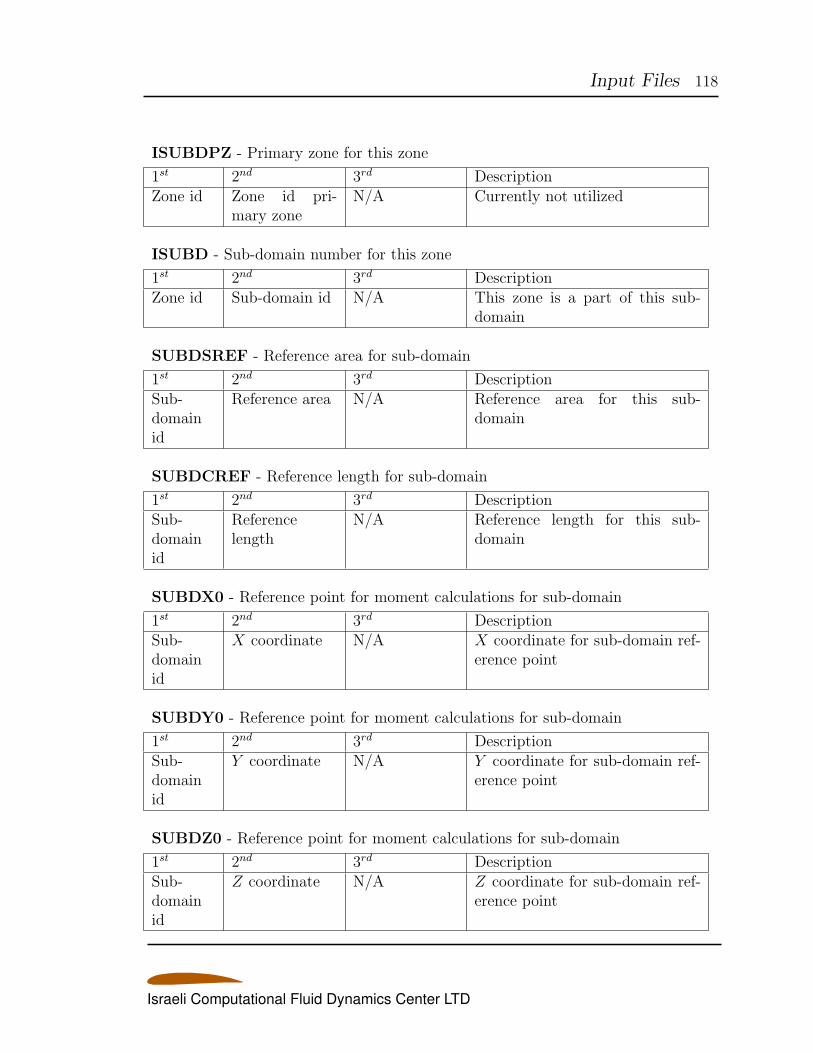
Input Files 118
ISUBDPZ - Primary zone for this zone
1st 2nd 3rd DescriptionZone id Zone id pri-
mary zoneN/A Currently not utilized
ISUBD - Sub-domain number for this zone
1st 2nd 3rd DescriptionZone id Sub-domain id N/A This zone is a part of this sub-
domain
SUBDSREF - Reference area for sub-domain
1st 2nd 3rd DescriptionSub-domainid
Reference area N/A Reference area for this sub-domain
SUBDCREF - Reference length for sub-domain
1st 2nd 3rd DescriptionSub-domainid
Referencelength
N/A Reference length for this sub-domain
SUBDX0 - Reference point for moment calculations for sub-domain
1st 2nd 3rd DescriptionSub-domainid
X coordinate N/A X coordinate for sub-domain ref-erence point
SUBDY0 - Reference point for moment calculations for sub-domain
1st 2nd 3rd DescriptionSub-domainid
Y coordinate N/A Y coordinate for sub-domain ref-erence point
SUBDZ0 - Reference point for moment calculations for sub-domain
1st 2nd 3rd DescriptionSub-domainid
Z coordinate N/A Z coordinate for sub-domain ref-erence point
Israeli Computational Fluid Dynamics Center LTD
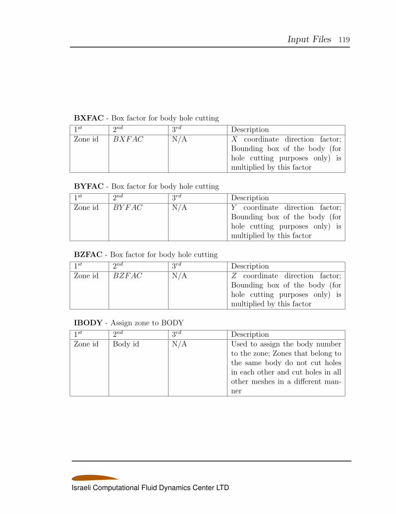
Input Files 119
BXFAC - Box factor for body hole cutting
1st 2nd 3rd DescriptionZone id BXFAC N/A X coordinate direction factor;
Bounding box of the body (forhole cutting purposes only) ismultiplied by this factor
BYFAC - Box factor for body hole cutting
1st 2nd 3rd DescriptionZone id BY FAC N/A Y coordinate direction factor;
Bounding box of the body (forhole cutting purposes only) ismultiplied by this factor
BZFAC - Box factor for body hole cutting
1st 2nd 3rd DescriptionZone id BZFAC N/A Z coordinate direction factor;
Bounding box of the body (forhole cutting purposes only) ismultiplied by this factor
IBODY - Assign zone to BODY
1st 2nd 3rd DescriptionZone id Body id N/A Used to assign the body number
to the zone; Zones that belong tothe same body do not cut holesin each other and cut holes in allother meshes in a different man-ner
Israeli Computational Fluid Dynamics Center LTD
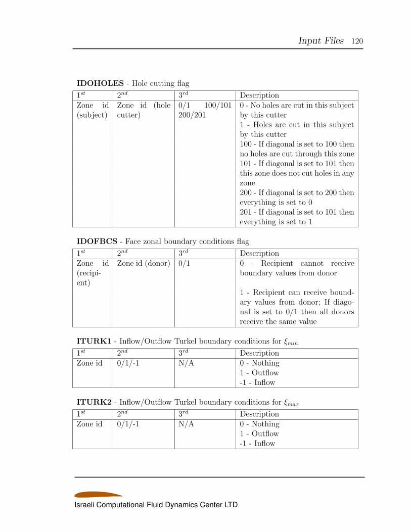
Input Files 120
IDOHOLES - Hole cutting flag
1st 2nd 3rd DescriptionZone id(subject)
Zone id (holecutter)
0/1 100/101200/201
0 - No holes are cut in this subjectby this cutter1 - Holes are cut in this subjectby this cutter100 - If diagonal is set to 100 thenno holes are cut through this zone101 - If diagonal is set to 101 thenthis zone does not cut holes in anyzone200 - If diagonal is set to 200 theneverything is set to 0201 - If diagonal is set to 101 theneverything is set to 1
IDOFBCS - Face zonal boundary conditions flag
1st 2nd 3rd DescriptionZone id(recipi-ent)
Zone id (donor) 0/1 0 - Recipient cannot receiveboundary values from donor
1 - Recipient can receive bound-ary values from donor; If diago-nal is set to 0/1 then all donorsreceive the same value
ITURK1 - Inflow/Outflow Turkel boundary conditions for ξmin
1st 2nd 3rd DescriptionZone id 0/1/-1 N/A 0 - Nothing
1 - Outflow-1 - Inflow
ITURK2 - Inflow/Outflow Turkel boundary conditions for ξmax
1st 2nd 3rd DescriptionZone id 0/1/-1 N/A 0 - Nothing
1 - Outflow-1 - Inflow
Israeli Computational Fluid Dynamics Center LTD
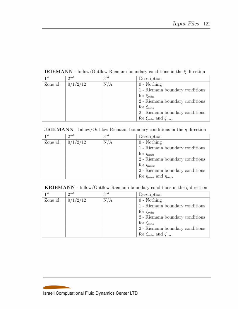
Input Files 121
IRIEMANN - Inflow/Outflow Riemann boundary conditions in the ξ direction
1st 2nd 3rd DescriptionZone id 0/1/2/12 N/A 0 - Nothing
1 - Riemann boundary conditionsfor ξmin
2 - Riemann boundary conditionsfor ξmax
2 - Riemann boundary conditionsfor ξmin and ξmax
JRIEMANN - Inflow/Outflow Riemann boundary conditions in the η direction
1st 2nd 3rd DescriptionZone id 0/1/2/12 N/A 0 - Nothing
1 - Riemann boundary conditionsfor ηmin
2 - Riemann boundary conditionsfor ηmax
2 - Riemann boundary conditionsfor ηmin and ηmax
KRIEMANN - Inflow/Outflow Riemann boundary conditions in the ζ direction
1st 2nd 3rd DescriptionZone id 0/1/2/12 N/A 0 - Nothing
1 - Riemann boundary conditionsfor ζmin
2 - Riemann boundary conditionsfor ζmax
2 - Riemann boundary conditionsfor ζmin and ζmax
Israeli Computational Fluid Dynamics Center LTD
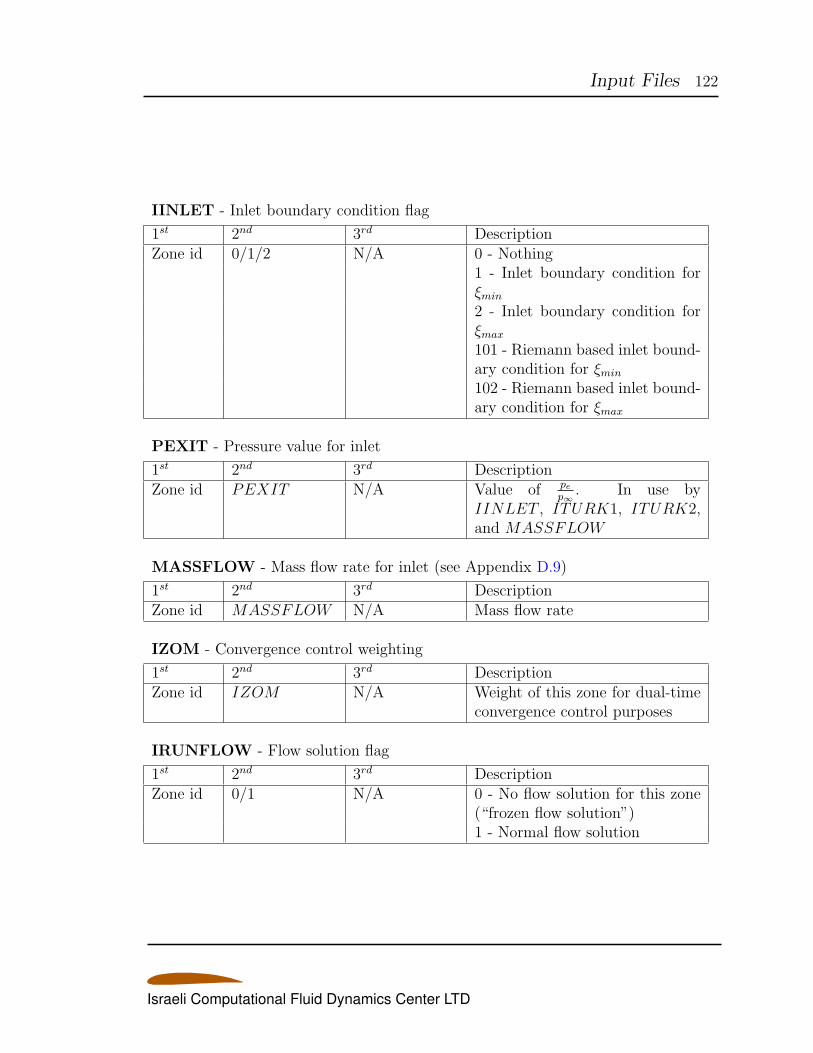
Input Files 122
IINLET - Inlet boundary condition flag
1st 2nd 3rd DescriptionZone id 0/1/2 N/A 0 - Nothing
1 - Inlet boundary condition forξmin
2 - Inlet boundary condition forξmax
101 - Riemann based inlet bound-ary condition for ξmin
102 - Riemann based inlet bound-ary condition for ξmax
PEXIT - Pressure value for inlet
1st 2nd 3rd DescriptionZone id PEXIT N/A Value of pe
p∞. In use by
IINLET , ITURK1, ITURK2,and MASSFLOW
MASSFLOW - Mass flow rate for inlet (see Appendix D.9)
1st 2nd 3rd DescriptionZone id MASSFLOW N/A Mass flow rate
IZOM - Convergence control weighting
1st 2nd 3rd DescriptionZone id IZOM N/A Weight of this zone for dual-time
convergence control purposes
IRUNFLOW - Flow solution flag
1st 2nd 3rd DescriptionZone id 0/1 N/A 0 - No flow solution for this zone
(“frozen flow solution”)1 - Normal flow solution
Israeli Computational Fluid Dynamics Center LTD
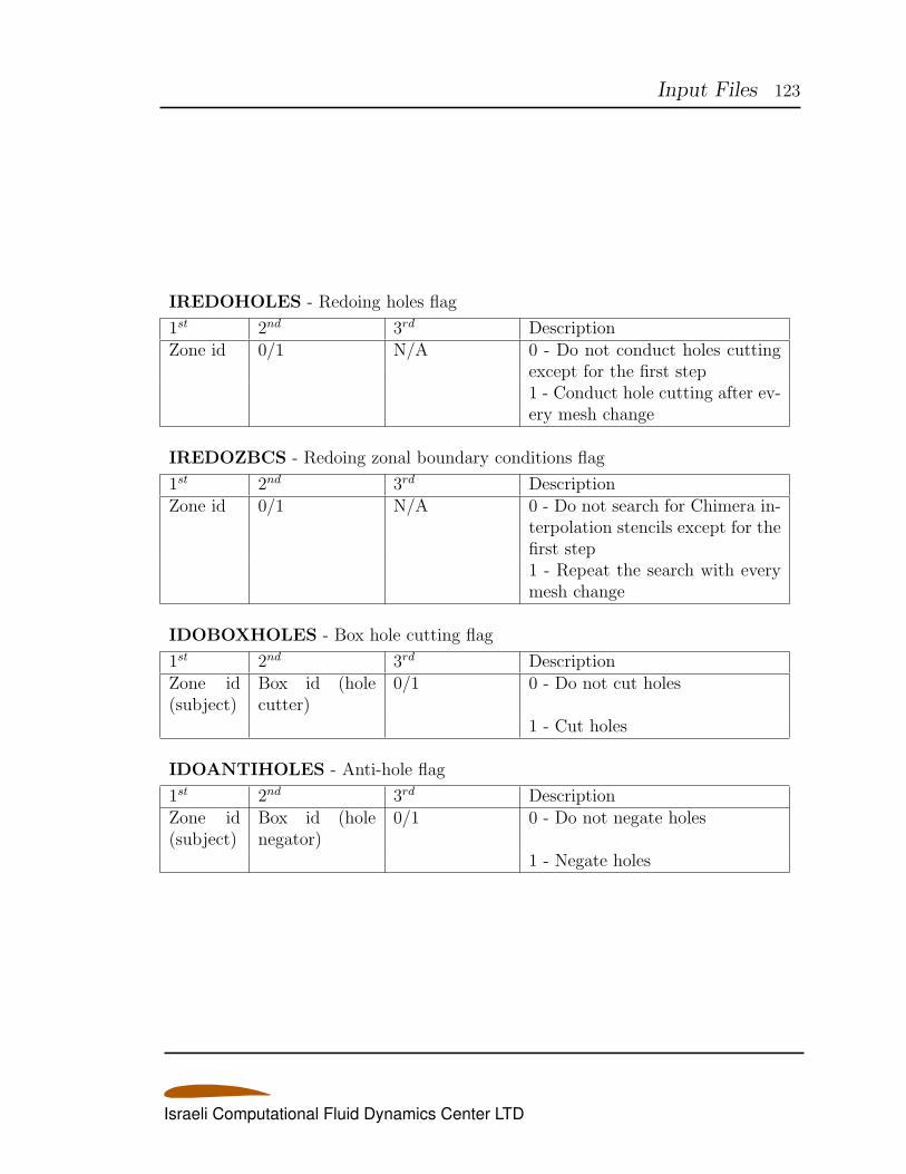
Input Files 123
IREDOHOLES - Redoing holes flag
1st 2nd 3rd DescriptionZone id 0/1 N/A 0 - Do not conduct holes cutting
except for the first step1 - Conduct hole cutting after ev-ery mesh change
IREDOZBCS - Redoing zonal boundary conditions flag
1st 2nd 3rd DescriptionZone id 0/1 N/A 0 - Do not search for Chimera in-
terpolation stencils except for thefirst step1 - Repeat the search with everymesh change
IDOBOXHOLES - Box hole cutting flag
1st 2nd 3rd DescriptionZone id(subject)
Box id (holecutter)
0/1 0 - Do not cut holes
1 - Cut holes
IDOANTIHOLES - Anti-hole flag
1st 2nd 3rd DescriptionZone id(subject)
Box id (holenegator)
0/1 0 - Do not negate holes
1 - Negate holes
Israeli Computational Fluid Dynamics Center LTD
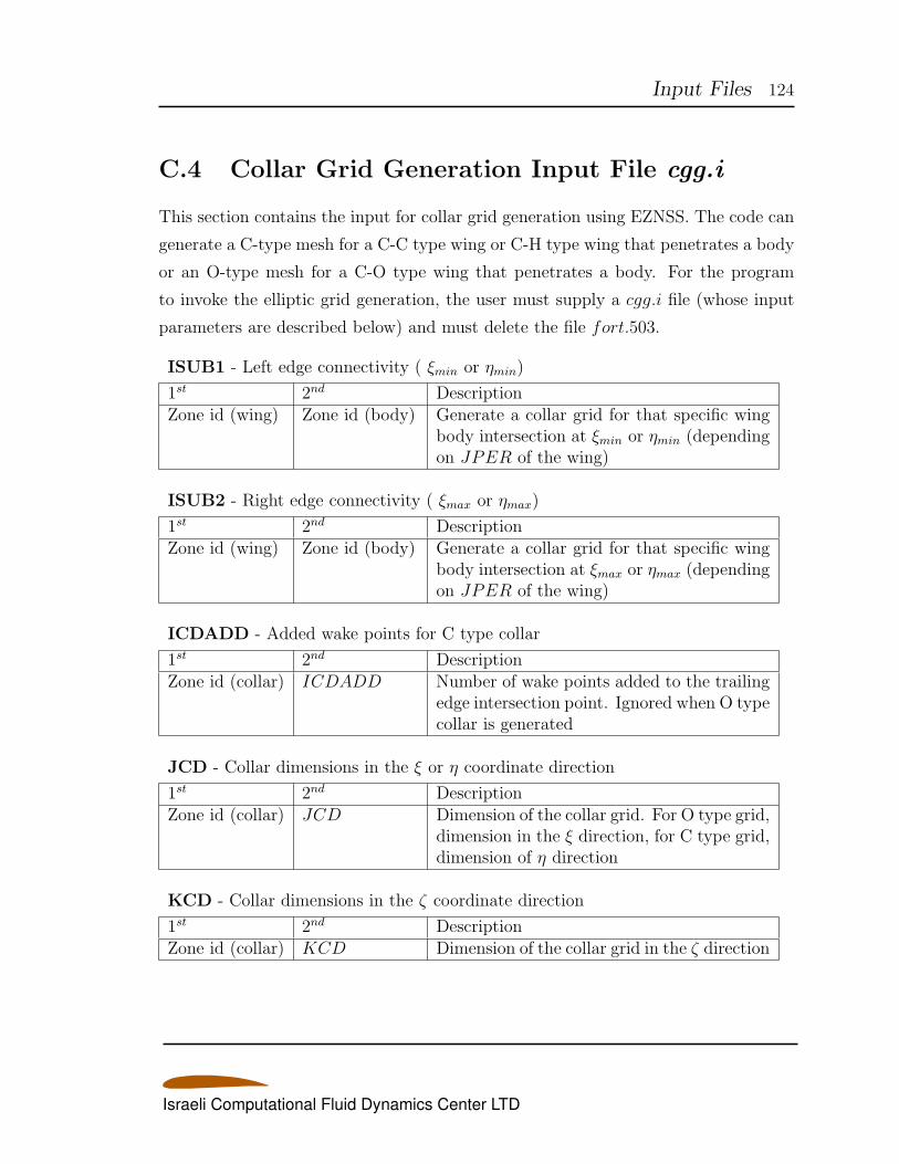
Input Files 124
C.4 Collar Grid Generation Input File cgg.i
This section contains the input for collar grid generation using EZNSS. The code can
generate a C-type mesh for a C-C type wing or C-H type wing that penetrates a body
or an O-type mesh for a C-O type wing that penetrates a body. For the program
to invoke the elliptic grid generation, the user must supply a cgg.i file (whose input
parameters are described below) and must delete the file fort.503.
ISUB1 - Left edge connectivity ( ξmin or ηmin)
1st 2nd DescriptionZone id (wing) Zone id (body) Generate a collar grid for that specific wing
body intersection at ξmin or ηmin (dependingon JPER of the wing)
ISUB2 - Right edge connectivity ( ξmax or ηmax)
1st 2nd DescriptionZone id (wing) Zone id (body) Generate a collar grid for that specific wing
body intersection at ξmax or ηmax (dependingon JPER of the wing)
ICDADD - Added wake points for C type collar
1st 2nd DescriptionZone id (collar) ICDADD Number of wake points added to the trailing
edge intersection point. Ignored when O typecollar is generated
JCD - Collar dimensions in the ξ or η coordinate direction
1st 2nd DescriptionZone id (collar) JCD Dimension of the collar grid. For O type grid,
dimension in the ξ direction, for C type grid,dimension of η direction
KCD - Collar dimensions in the ζ coordinate direction
1st 2nd DescriptionZone id (collar) KCD Dimension of the collar grid in the ζ direction
Israeli Computational Fluid Dynamics Center LTD
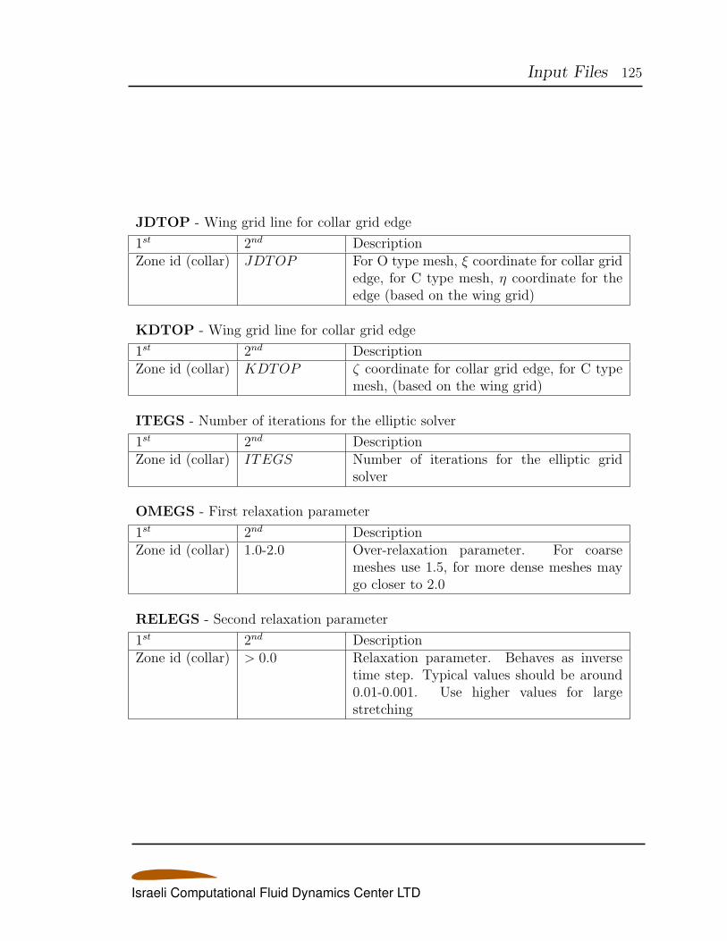
Input Files 125
JDTOP - Wing grid line for collar grid edge
1st 2nd DescriptionZone id (collar) JDTOP For O type mesh, ξ coordinate for collar grid
edge, for C type mesh, η coordinate for theedge (based on the wing grid)
KDTOP - Wing grid line for collar grid edge
1st 2nd DescriptionZone id (collar) KDTOP ζ coordinate for collar grid edge, for C type
mesh, (based on the wing grid)
ITEGS - Number of iterations for the elliptic solver
1st 2nd DescriptionZone id (collar) ITEGS Number of iterations for the elliptic grid
solver
OMEGS - First relaxation parameter
1st 2nd DescriptionZone id (collar) 1.0-2.0 Over-relaxation parameter. For coarse
meshes use 1.5, for more dense meshes maygo closer to 2.0
RELEGS - Second relaxation parameter
1st 2nd DescriptionZone id (collar) > 0.0 Relaxation parameter. Behaves as inverse
time step. Typical values should be around0.01-0.001. Use higher values for largestretching
Israeli Computational Fluid Dynamics Center LTD
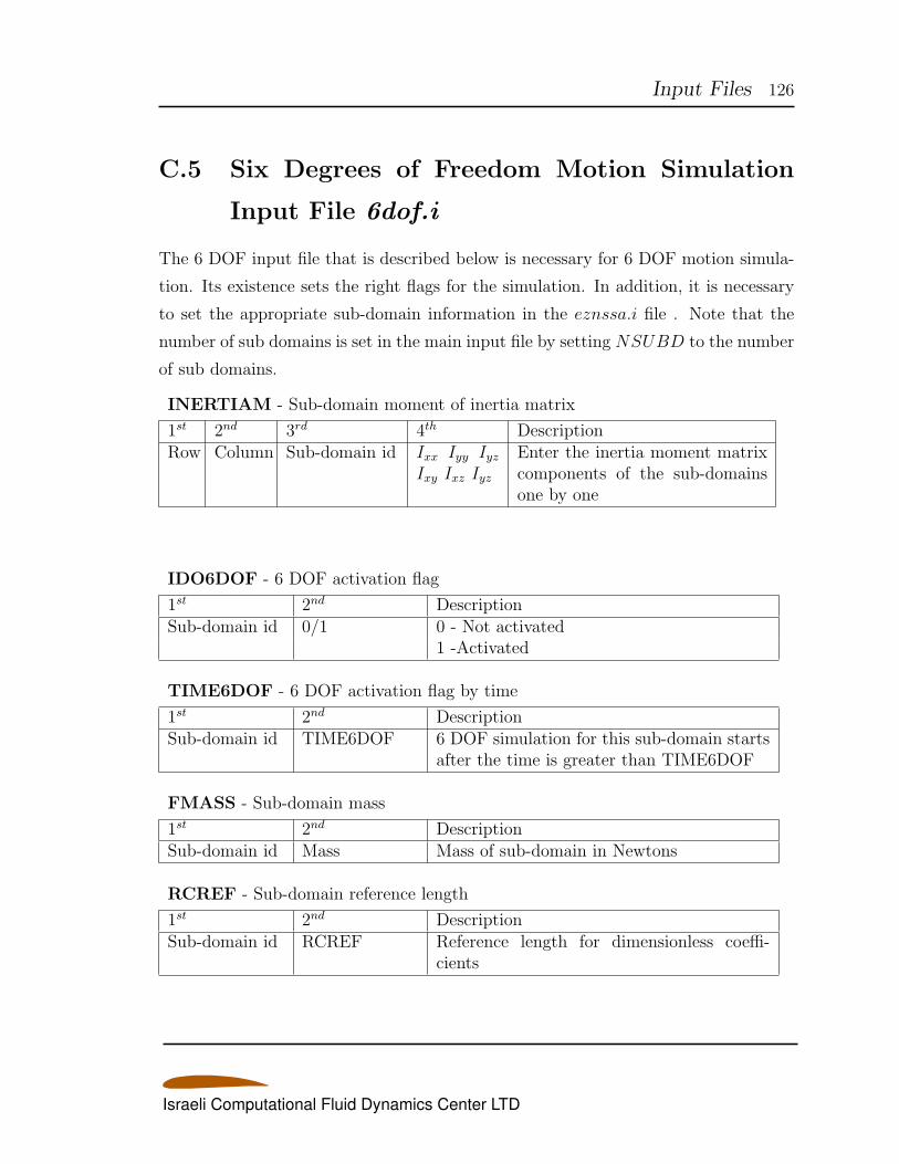
Input Files 126
C.5 Six Degrees of Freedom Motion Simulation
Input File 6dof.i
The 6 DOF input file that is described below is necessary for 6 DOF motion simula-
tion. Its existence sets the right flags for the simulation. In addition, it is necessary
to set the appropriate sub-domain information in the eznssa.i file . Note that the
number of sub domains is set in the main input file by setting NSUBD to the number
of sub domains.
INERTIAM - Sub-domain moment of inertia matrix
1st 2nd 3rd 4th DescriptionRow Column Sub-domain id Ixx Iyy Iyz
Ixy Ixz Iyz
Enter the inertia moment matrixcomponents of the sub-domainsone by one
IDO6DOF - 6 DOF activation flag
1st 2nd DescriptionSub-domain id 0/1 0 - Not activated
1 -Activated
TIME6DOF - 6 DOF activation flag by time
1st 2nd DescriptionSub-domain id TIME6DOF 6 DOF simulation for this sub-domain starts
after the time is greater than TIME6DOF
FMASS - Sub-domain mass
1st 2nd DescriptionSub-domain id Mass Mass of sub-domain in Newtons
RCREF - Sub-domain reference length
1st 2nd DescriptionSub-domain id RCREF Reference length for dimensionless coeffi-
cients
Israeli Computational Fluid Dynamics Center LTD
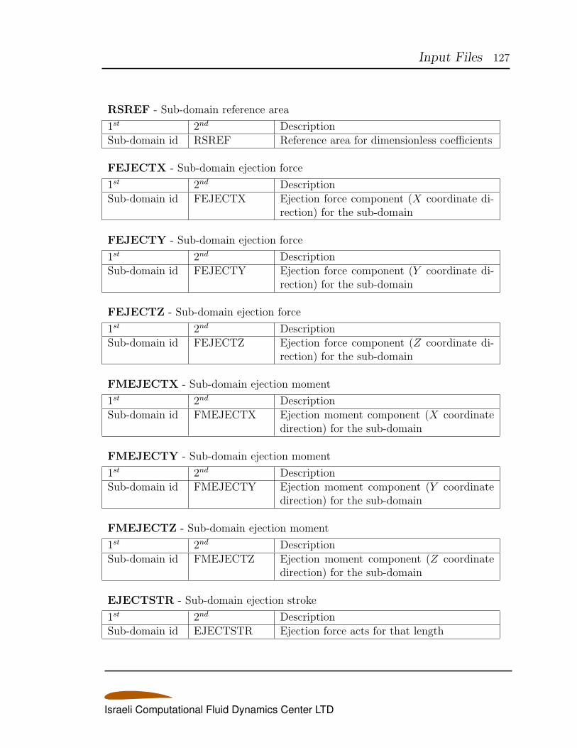
Input Files 127
RSREF - Sub-domain reference area
1st 2nd DescriptionSub-domain id RSREF Reference area for dimensionless coefficients
FEJECTX - Sub-domain ejection force
1st 2nd DescriptionSub-domain id FEJECTX Ejection force component (X coordinate di-
rection) for the sub-domain
FEJECTY - Sub-domain ejection force
1st 2nd DescriptionSub-domain id FEJECTY Ejection force component (Y coordinate di-
rection) for the sub-domain
FEJECTZ - Sub-domain ejection force
1st 2nd DescriptionSub-domain id FEJECTZ Ejection force component (Z coordinate di-
rection) for the sub-domain
FMEJECTX - Sub-domain ejection moment
1st 2nd DescriptionSub-domain id FMEJECTX Ejection moment component (X coordinate
direction) for the sub-domain
FMEJECTY - Sub-domain ejection moment
1st 2nd DescriptionSub-domain id FMEJECTY Ejection moment component (Y coordinate
direction) for the sub-domain
FMEJECTZ - Sub-domain ejection moment
1st 2nd DescriptionSub-domain id FMEJECTZ Ejection moment component (Z coordinate
direction) for the sub-domain
EJECTSTR - Sub-domain ejection stroke
1st 2nd DescriptionSub-domain id EJECTSTR Ejection force acts for that length
Israeli Computational Fluid Dynamics Center LTD
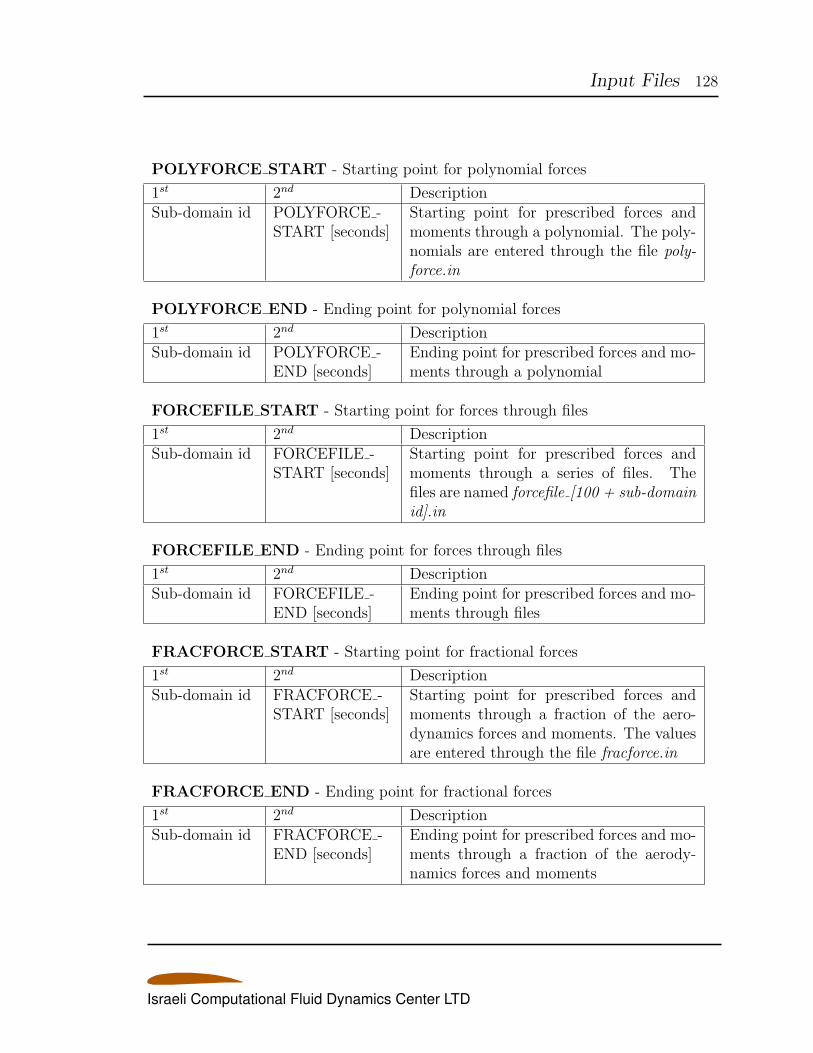
Input Files 128
POLYFORCE START - Starting point for polynomial forces
1st 2nd DescriptionSub-domain id POLYFORCE -
START [seconds]Starting point for prescribed forces andmoments through a polynomial. The poly-nomials are entered through the file poly-force.in
POLYFORCE END - Ending point for polynomial forces
1st 2nd DescriptionSub-domain id POLYFORCE -
END [seconds]Ending point for prescribed forces and mo-ments through a polynomial
FORCEFILE START - Starting point for forces through files
1st 2nd DescriptionSub-domain id FORCEFILE -
START [seconds]Starting point for prescribed forces andmoments through a series of files. Thefiles are named forcefile [100 + sub-domainid].in
FORCEFILE END - Ending point for forces through files
1st 2nd DescriptionSub-domain id FORCEFILE -
END [seconds]Ending point for prescribed forces and mo-ments through files
FRACFORCE START - Starting point for fractional forces
1st 2nd DescriptionSub-domain id FRACFORCE -
START [seconds]Starting point for prescribed forces andmoments through a fraction of the aero-dynamics forces and moments. The valuesare entered through the file fracforce.in
FRACFORCE END - Ending point for fractional forces
1st 2nd DescriptionSub-domain id FRACFORCE -
END [seconds]Ending point for prescribed forces and mo-ments through a fraction of the aerody-namics forces and moments
Israeli Computational Fluid Dynamics Center LTD
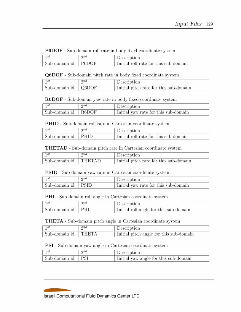
Input Files 129
P6DOF - Sub-domain roll rate in body fixed coordinate system
1st 2nd DescriptionSub-domain id P6DOF Initial roll rate for this sub-domain
Q6DOF - Sub-domain pitch rate in body fixed coordinate system
1st 2nd DescriptionSub-domain id Q6DOF Initial pitch rate for this sub-domain
R6DOF - Sub-domain yaw rate in body fixed coordinate system
1st 2nd DescriptionSub-domain id R6DOF Initial yaw rate for this sub-domain
PHID - Sub-domain roll rate in Cartesian coordinate system
1st 2nd DescriptionSub-domain id PHID Initial roll rate for this sub-domain
THETAD - Sub-domain pitch rate in Cartesian coordinate system
1st 2nd DescriptionSub-domain id THETAD Initial pitch rate for this sub-domain
PSID - Sub-domain yaw rate in Cartesian coordinate system
1st 2nd DescriptionSub-domain id PSID Initial yaw rate for this sub-domain
PHI - Sub-domain roll angle in Cartesian coordinate system
1st 2nd DescriptionSub-domain id PHI Initial roll angle for this sub-domain
THETA - Sub-domain pitch angle in Cartesian coordinate system
1st 2nd DescriptionSub-domain id THETA Initial pitch angle for this sub-domain
PSI - Sub-domain yaw angle in Cartesian coordinate system
1st 2nd DescriptionSub-domain id PSI Initial yaw angle for this sub-domain
Israeli Computational Fluid Dynamics Center LTD
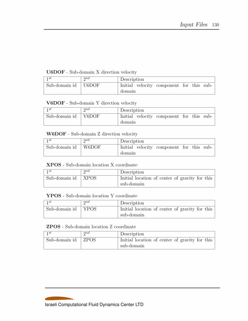
Input Files 130
U6DOF - Sub-domain X direction velocity
1st 2nd DescriptionSub-domain id U6DOF Initial velocity component for this sub-
domain
V6DOF - Sub-domain Y direction velocity
1st 2nd DescriptionSub-domain id V6DOF Initial velocity component for this sub-
domain
W6DOF - Sub-domain Z direction velocity
1st 2nd DescriptionSub-domain id W6DOF Initial velocity component for this sub-
domain
XPOS - Sub-domain location X coordinate
1st 2nd DescriptionSub-domain id XPOS Initial location of center of gravity for this
sub-domain
YPOS - Sub-domain location Y coordinate
1st 2nd DescriptionSub-domain id YPOS Initial location of center of gravity for this
sub-domain
ZPOS - Sub-domain location Z coordinate
1st 2nd DescriptionSub-domain id ZPOS Initial location of center of gravity for this
sub-domain
Israeli Computational Fluid Dynamics Center LTD
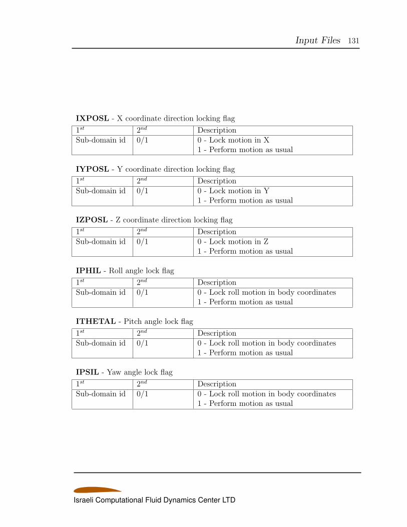
Input Files 131
IXPOSL - X coordinate direction locking flag
1st 2nd DescriptionSub-domain id 0/1 0 - Lock motion in X
1 - Perform motion as usual
IYPOSL - Y coordinate direction locking flag
1st 2nd DescriptionSub-domain id 0/1 0 - Lock motion in Y
1 - Perform motion as usual
IZPOSL - Z coordinate direction locking flag
1st 2nd DescriptionSub-domain id 0/1 0 - Lock motion in Z
1 - Perform motion as usual
IPHIL - Roll angle lock flag
1st 2nd DescriptionSub-domain id 0/1 0 - Lock roll motion in body coordinates
1 - Perform motion as usual
ITHETAL - Pitch angle lock flag
1st 2nd DescriptionSub-domain id 0/1 0 - Lock roll motion in body coordinates
1 - Perform motion as usual
IPSIL - Yaw angle lock flag
1st 2nd DescriptionSub-domain id 0/1 0 - Lock roll motion in body coordinates
1 - Perform motion as usual
Israeli Computational Fluid Dynamics Center LTD
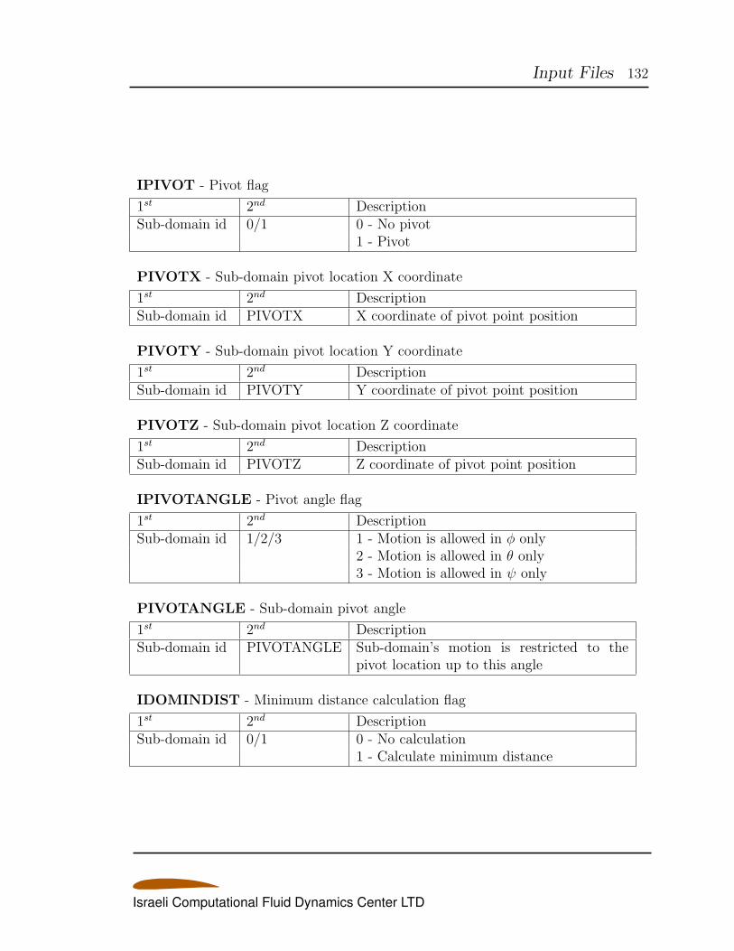
Input Files 132
IPIVOT - Pivot flag
1st 2nd DescriptionSub-domain id 0/1 0 - No pivot
1 - Pivot
PIVOTX - Sub-domain pivot location X coordinate
1st 2nd DescriptionSub-domain id PIVOTX X coordinate of pivot point position
PIVOTY - Sub-domain pivot location Y coordinate
1st 2nd DescriptionSub-domain id PIVOTY Y coordinate of pivot point position
PIVOTZ - Sub-domain pivot location Z coordinate
1st 2nd DescriptionSub-domain id PIVOTZ Z coordinate of pivot point position
IPIVOTANGLE - Pivot angle flag
1st 2nd DescriptionSub-domain id 1/2/3 1 - Motion is allowed in ϕ only
2 - Motion is allowed in θ only3 - Motion is allowed in ψ only
PIVOTANGLE - Sub-domain pivot angle
1st 2nd DescriptionSub-domain id PIVOTANGLE Sub-domain’s motion is restricted to the
pivot location up to this angle
IDOMINDIST - Minimum distance calculation flag
1st 2nd DescriptionSub-domain id 0/1 0 - No calculation
1 - Calculate minimum distance
Israeli Computational Fluid Dynamics Center LTD
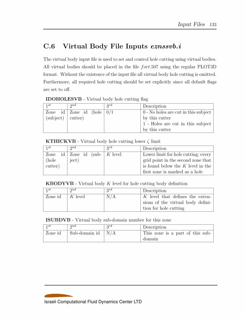
Input Files 133
C.6 Virtual Body File Inputs eznssvb.i
The virtual body input file is used to set and control hole cutting using virtual bodies.
All virtual bodies should be placed in the file fort.507 using the regular PLOT3D
format. Without the existence of the input file all virtual body hole cutting is omitted.
Furthermore, all required hole cutting should be set explicitly since all default flags
are set to off.
IDOHOLESVB - Virtual body hole cutting flag
1st 2nd 3rd DescriptionZone id(subject)
Zone id (holecutter)
0/1 0 - No holes are cut in this subjectby this cutter1 - Holes are cut in this subjectby this cutter
KTHICKVB - Virtual body hole cutting lower ζ limit
1st 2nd 3rd DescriptionZone id(holecutter)
Zone id (sub-ject)
K level Lower limit for hole cutting; everygrid point in the second zone thatis found below the K level in thefirst zone is marked as a hole
KBODYVB - Virtual body K level for hole cutting body definition
1st 2nd 3rd DescriptionZone id K level N/A K level that defines the exten-
sions of the virtual body defini-tion for hole cutting
ISUBDVB - Virtual body sub-domain number for this zone
1st 2nd 3rd DescriptionZone id Sub-domain id N/A This zone is a part of this sub-
domain
Israeli Computational Fluid Dynamics Center LTD
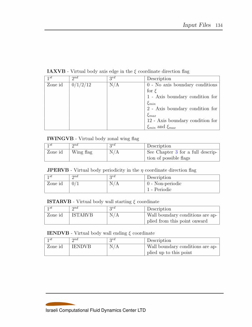
Input Files 134
IAXVB - Virtual body axis edge in the ξ coordinate direction flag
1st 2nd 3rd DescriptionZone id 0/1/2/12 N/A 0 - No axis boundary conditions
for ξ1 - Axis boundary condition forξmin
2 - Axis boundary condition forξmax
12 - Axis boundary condition forξmin and ξmax
IWINGVB - Virtual body zonal wing flag
1st 2nd 3rd DescriptionZone id Wing flag N/A See Chapter 3 for a full descrip-
tion of possible flags
JPERVB - Virtual body periodicity in the η coordinate direction flag
1st 2nd 3rd DescriptionZone id 0/1 N/A 0 - Non-periodic
1 - Periodic
ISTARVB - Virtual body wall starting ξ coordinate
1st 2nd 3rd DescriptionZone id ISTARVB N/A Wall boundary conditions are ap-
plied from this point onward
IENDVB - Virtual body wall ending ξ coordinate
1st 2nd 3rd DescriptionZone id IENDVB N/A Wall boundary conditions are ap-
plied up to this point
Israeli Computational Fluid Dynamics Center LTD
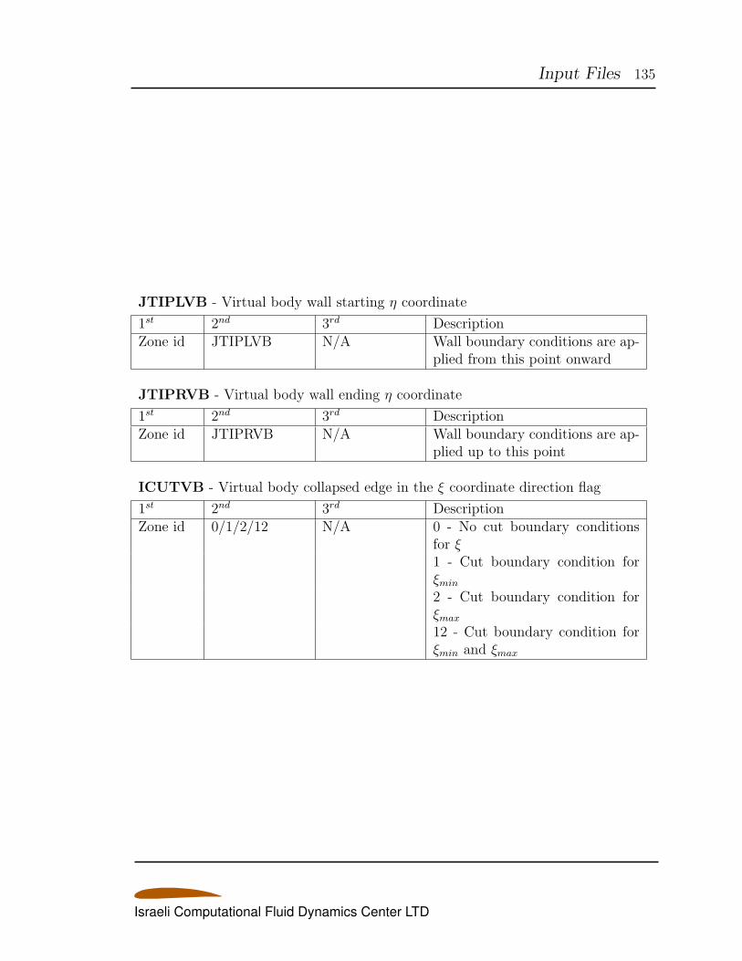
Input Files 135
JTIPLVB - Virtual body wall starting η coordinate
1st 2nd 3rd DescriptionZone id JTIPLVB N/A Wall boundary conditions are ap-
plied from this point onward
JTIPRVB - Virtual body wall ending η coordinate
1st 2nd 3rd DescriptionZone id JTIPRVB N/A Wall boundary conditions are ap-
plied up to this point
ICUTVB - Virtual body collapsed edge in the ξ coordinate direction flag
1st 2nd 3rd DescriptionZone id 0/1/2/12 N/A 0 - No cut boundary conditions
for ξ1 - Cut boundary condition forξmin
2 - Cut boundary condition forξmax
12 - Cut boundary condition forξmin and ξmax
Israeli Computational Fluid Dynamics Center LTD
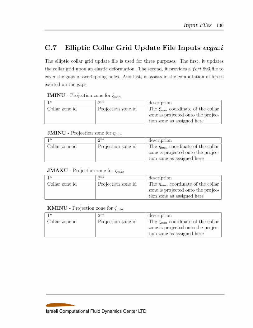
Input Files 136
C.7 Elliptic Collar Grid Update File Inputs ecgu.i
The elliptic collar grid update file is used for three purposes. The first, it updates
the collar grid upon an elastic deformation. The second, it provides a fort.893 file to
cover the gaps of overlapping holes. And last, it assists in the computation of forces
exerted on the gaps.
IMINU - Projection zone for ξmin
1st 2nd descriptionCollar zone id Projection zone id The ξmin coordinate of the collar
zone is projected onto the projec-tion zone as assigned here
JMINU - Projection zone for ηmin
1st 2nd descriptionCollar zone id Projection zone id The ηmin coordinate of the collar
zone is projected onto the projec-tion zone as assigned here
JMAXU - Projection zone for ηmax
1st 2nd descriptionCollar zone id Projection zone id The ηmax coordinate of the collar
zone is projected onto the projec-tion zone as assigned here
KMINU - Projection zone for ζmin
1st 2nd descriptionCollar zone id Projection zone id The ζmin coordinate of the collar
zone is projected onto the projec-tion zone as assigned here
Israeli Computational Fluid Dynamics Center LTD
Input Files 137
C.8 Spline Inputs in File spline.i
File spline.i includes the input data required for mapping the elastic modes from the
structural grid in which they are provided to the aerodynamic grid. The required
data includes: for each structural surface the type of spline (surface/beam); for each
aerodynamic surface the corresponding structural surface for spline; displacements
and rotations applied to the aerodynamic surface to align it with the structural sur-
faces (for spline purposes only), and plot factors for displaying the mapped modes.
Each variable has two entries described below.
For cases of constrained deformations, in which subdomains are connected rigidly
to a single point and are constrained to move rigidly with that point, the constraint
points (one for each such sub-domain) are defined via their x,y, and z coordinates,
and by the aerodynamic grid zone to which each sub-domain attaches.
Israeli Computational Fluid Dynamics Center LTD
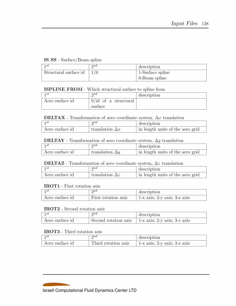
Input Files 138
IS SS - Surface/Beam spline
1st 2nd descriptionStructural surface id 1/0 1-Surface spline
0-Beam spline
ISPLINE FROM - Which structural surface to spline from1st 2nd descriptionAero surface id 0/id of a structural
surface
DELTAX - Transformation of aero coordinate system, ∆x translation1st 2nd descriptionAero surface id translation ∆x in length units of the aero grid
DELTAY - Transformation of aero coordinate system, ∆y translation1st 2nd descriptionAero surface id translation ∆y in length units of the aero grid
DELTAZ - Transformation of aero coordinate system, ∆z translation1st 2nd descriptionAero surface id translation ∆z in length units of the aero grid
IROT1 - First rotation axis1st 2nd descriptionAero surface id First rotation axis 1-x axis; 2-y axis; 3-z axis
IROT2 - Second rotation axis1st 2nd descriptionAero surface id Second rotation axis 1-x axis; 2-y axis; 3-z axis
IROT3 - Third rotation axis1st 2nd descriptionAero surface id Third rotation axis 1-x axis; 2-y axis; 3-z axis
Israeli Computational Fluid Dynamics Center LTD
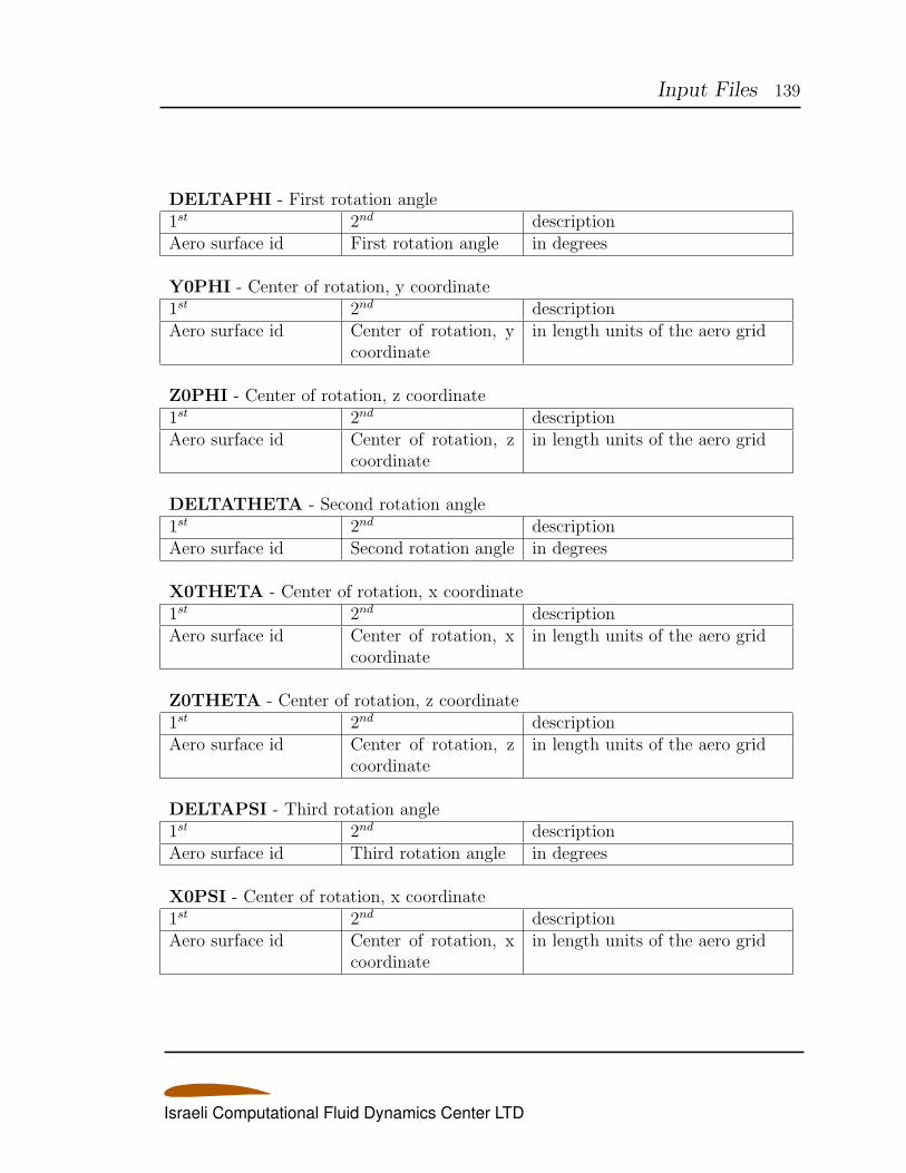
Input Files 139
DELTAPHI - First rotation angle1st 2nd descriptionAero surface id First rotation angle in degrees
Y0PHI - Center of rotation, y coordinate1st 2nd descriptionAero surface id Center of rotation, y
coordinatein length units of the aero grid
Z0PHI - Center of rotation, z coordinate1st 2nd descriptionAero surface id Center of rotation, z
coordinatein length units of the aero grid
DELTATHETA - Second rotation angle1st 2nd descriptionAero surface id Second rotation angle in degrees
X0THETA - Center of rotation, x coordinate1st 2nd descriptionAero surface id Center of rotation, x
coordinatein length units of the aero grid
Z0THETA - Center of rotation, z coordinate1st 2nd descriptionAero surface id Center of rotation, z
coordinatein length units of the aero grid
DELTAPSI - Third rotation angle1st 2nd descriptionAero surface id Third rotation angle in degrees
X0PSI - Center of rotation, x coordinate1st 2nd descriptionAero surface id Center of rotation, x
coordinatein length units of the aero grid
Israeli Computational Fluid Dynamics Center LTD
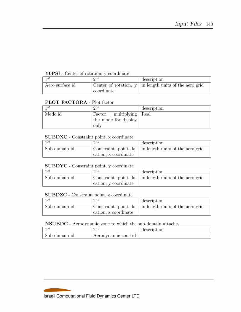
Input Files 140
Y0PSI - Center of rotation, y coordinate1st 2nd descriptionAero surface id Center of rotation, y
coordinatein length units of the aero grid
PLOT FACTORA - Plot factor1st 2nd descriptionMode id Factor multiplying
the mode for displayonly
Real
SUBDXC - Constraint point, x coordinate1st 2nd descriptionSub-domain id Constraint point lo-
cation, x coordinatein length units of the aero grid
SUBDYC - Constraint point, y coordinate1st 2nd descriptionSub-domain id Constraint point lo-
cation, y coordinatein length units of the aero grid
SUBDZC - Constraint point, z coordinate1st 2nd descriptionSub-domain id Constraint point lo-
cation, z coordinatein length units of the aero grid
NSUBDC - Aerodynamic zone to which the sub-domain attaches1st 2nd descriptionSub-domain id Aerodynamic zone id
Israeli Computational Fluid Dynamics Center LTD
Input Files 141
C.9 Flap Inputs in File flap.i
File flap.i includes the input data required for defining leading and trailing edge
control surfaces. The required data includes: Dimensions of a fictitious mesh on
which flap deflections are defined; for each flap - which aerodynamic zone it belongs
to, is the flap a leading/trailing edge flap, definition of the flap hinge (x,y coordinates
of the flap hinge at the root side and at the tip side), flap deflection.
Israeli Computational Fluid Dynamics Center LTD
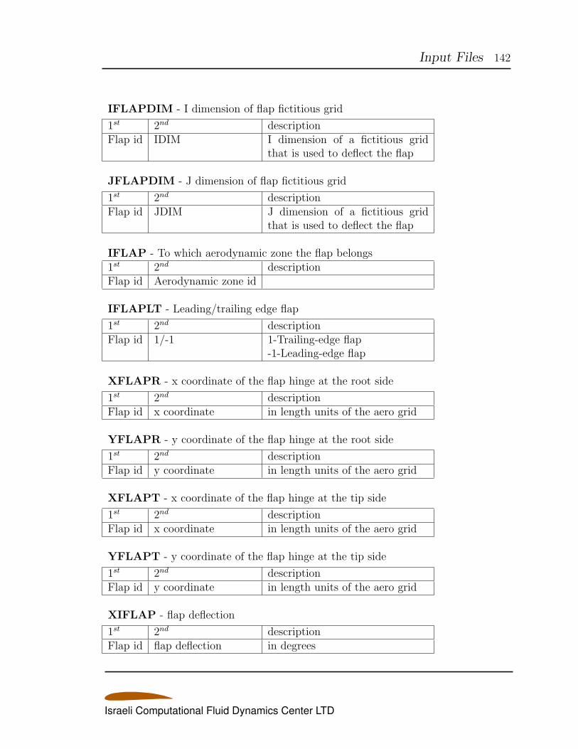
Input Files 142
IFLAPDIM - I dimension of flap fictitious grid
1st 2nd descriptionFlap id IDIM I dimension of a fictitious grid
that is used to deflect the flap
JFLAPDIM - J dimension of flap fictitious grid
1st 2nd descriptionFlap id JDIM J dimension of a fictitious grid
that is used to deflect the flap
IFLAP - To which aerodynamic zone the flap belongs1st 2nd descriptionFlap id Aerodynamic zone id
IFLAPLT - Leading/trailing edge flap
1st 2nd descriptionFlap id 1/-1 1-Trailing-edge flap
-1-Leading-edge flap
XFLAPR - x coordinate of the flap hinge at the root side
1st 2nd descriptionFlap id x coordinate in length units of the aero grid
YFLAPR - y coordinate of the flap hinge at the root side
1st 2nd descriptionFlap id y coordinate in length units of the aero grid
XFLAPT - x coordinate of the flap hinge at the tip side
1st 2nd descriptionFlap id x coordinate in length units of the aero grid
YFLAPT - y coordinate of the flap hinge at the tip side
1st 2nd descriptionFlap id y coordinate in length units of the aero grid
XIFLAP - flap deflection
1st 2nd descriptionFlap id flap deflection in degrees
Israeli Computational Fluid Dynamics Center LTD
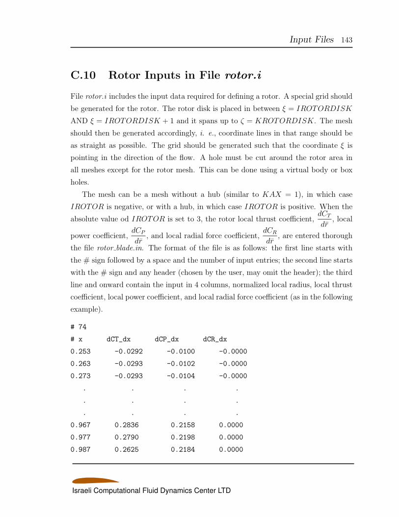
Input Files 143
C.10 Rotor Inputs in File rotor.i
File rotor.i includes the input data required for defining a rotor. A special grid should
be generated for the rotor. The rotor disk is placed in between ξ = IROTORDISK
AND ξ = IROTORDISK + 1 and it spans up to ζ = KROTORDISK. The mesh
should then be generated accordingly, i. e., coordinate lines in that range should be
as straight as possible. The grid should be generated such that the coordinate ξ is
pointing in the direction of the flow. A hole must be cut around the rotor area in
all meshes except for the rotor mesh. This can be done using a virtual body or box
holes.
The mesh can be a mesh without a hub (similar to KAX = 1), in which case
IROTOR is negative, or with a hub, in which case IROTOR is positive. When the
absolute value od IROTOR is set to 3, the rotor local thrust coefficient,dCT
dr, local
power coefficient,dCP
dr, and local radial force coefficient,
dCR
dr, are entered thorough
the file rotor blade.in. The format of the file is as follows: the first line starts with
the # sign followed by a space and the number of input entries; the second line starts
with the # sign and any header (chosen by the user, may omit the header); the third
line and onward contain the input in 4 columns, normalized local radius, local thrust
coefficient, local power coefficient, and local radial force coefficient (as in the following
example).
# 74
# x dCT_dx dCP_dx dCR_dx
0.253 -0.0292 -0.0100 -0.0000
0.263 -0.0293 -0.0102 -0.0000
0.273 -0.0293 -0.0104 -0.0000
. . . .
. . . .
. . . .
0.967 0.2836 0.2158 0.0000
0.977 0.2790 0.2198 0.0000
0.987 0.2625 0.2184 0.0000
Israeli Computational Fluid Dynamics Center LTD
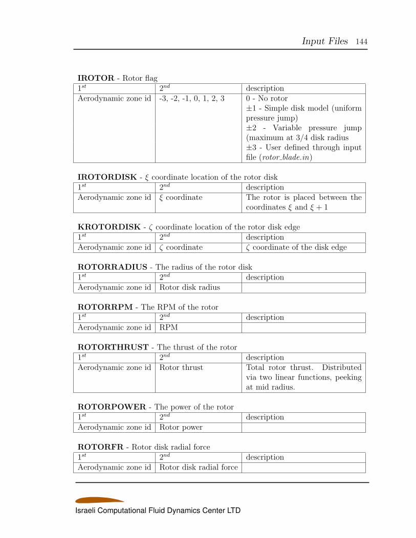
Input Files 144
IROTOR - Rotor flag1st 2nd descriptionAerodynamic zone id -3, -2, -1, 0, 1, 2, 3 0 - No rotor
±1 - Simple disk model (uniformpressure jump)±2 - Variable pressure jump(maximum at 3/4 disk radius±3 - User defined through inputfile (rotor blade.in)
IROTORDISK - ξ coordinate location of the rotor disk1st 2nd descriptionAerodynamic zone id ξ coordinate The rotor is placed between the
coordinates ξ and ξ + 1
KROTORDISK - ζ coordinate location of the rotor disk edge1st 2nd descriptionAerodynamic zone id ζ coordinate ζ coordinate of the disk edge
ROTORRADIUS - The radius of the rotor disk1st 2nd descriptionAerodynamic zone id Rotor disk radius
ROTORRPM - The RPM of the rotor1st 2nd descriptionAerodynamic zone id RPM
ROTORTHRUST - The thrust of the rotor1st 2nd descriptionAerodynamic zone id Rotor thrust Total rotor thrust. Distributed
via two linear functions, peekingat mid radius.
ROTORPOWER - The power of the rotor1st 2nd descriptionAerodynamic zone id Rotor power
ROTORFR - Rotor disk radial force1st 2nd descriptionAerodynamic zone id Rotor disk radial force
Israeli Computational Fluid Dynamics Center LTD
145
Appendix D
Data Files
D.1 Rationale
There are two main types of files, numbered files based on specific series and files that
are identified by names. Numbered data files are numbered according to the following
rationale. Single and double digit files contain global time history information. Triple
digit files are grid, solution, and other input/output files. Quadruple digit files contain
time history of the results of six degrees of freedom simulation and time history of
forces and moments.
D.2 Input Data Files
Grid files are named fort.501 - fort.505. The file fort.501 contains Chimera grids, the
file fort.502 contains patched grids, the file fort.503 contains elliptic collar grids, the
file fort.504 contains hyperbolic collar grids, and the file fort.505 contains Cartesian
grids. Another grid file, the virtual body grid file (named fort.507), is used to
define bodies for hole cutting. These bodies are not involved in the actual flow
calculations and their use is limited for the process of hole cutting only. Solution
files are named fort.511 - fort.515 where fort.511 is the solution file for grid file
fort.501 and so forth. Turbulent viscosity files are named fort.521 - fort.525, Rt
files are named fort.531 - fort.535 and γ files are named fort.541 - fort.545. The files
Israeli Computational Fluid Dynamics Center LTD
Data Files 146
fort.551 - fort.555 and fort.561 - fort.565 contain restart grid metrics for moving
grid computations. The files fort.571 - fort.575 contain wall distances.
In addition to the above files, there are two input files for static and dynamic
aeroelastic flow simulations. The file fort.800 contains the modes and eigenvalues,
whereas the file fort.808 contains initial modes and general forces.
D.3 Output Data Files
All files from the fort.500 series have corresponding output files that are names
fort.600 having exactly the last two digits. For example, the output γ file for an
elliptic collar grid would be names fort.643. When holes are generated a new series
of files is generated and is named fort.791, fort.792, and/or fort.795, depending on
the the corresponding grid file. The output file for aeroelastic modes and generalized
forces is named fort.818 (or fort.817 in case of a stop MONITOR command; in
that case the grid and solution files are named fort.26 and fort.27, respectively).
Convergence history is written into the files fort.7 (time vs. means square) and
fort.11 (iteration number vs. root mean square) and forces and moments time history
are written into the file fort.17. The format of the files fort.7 and fort.11 is the
time (or iteration number for fort.11) and L2NORM (or√L2NORM) for the file
fort.11) for all zones. The file fort.17 contains the time and then CX , CY , CZ , CMX,
CMY , CMZ, CL, and CD. Note, forces and moments in the fort.17 file are sums of
all forces and moments in all the zones.
The quadruple digit file series that correspond to sub-domains is numbered by
sub-domains (last 1, 2, or 3 digits). The fort.1000 series contain trajectory time
history, the fort.2000 series contain velocity time history, the fort.3000 series contain
the acceleration time history. The fort.8000 series contains forces and moments in
Cartesian coordinates while the fort.9000 series contains forces and moments in body
coordinates.
In addition, the fort.7000 file series contains time history for each zone, in a Carte-
sian coordinate system. The fort.804 file series contains modal deflections in forms of
surface grid files (this happens only when the input parameter ITER ELAT STAGE
Israeli Computational Fluid Dynamics Center LTD
Data Files 147
parameter is negative; the program stops after that). The fort.5000 series contains
surface collar grids for the possible generation of hyperbolic collar grids.
Convergence of sub-iterations in dual-time-stepping mode is reported in the fort.6000
file series. Each line of the file contains 8 columns. The first column is the time, the
second column is the number of sub-iteration that has been conducted, the next pair
of columns contain the residual drop of the mean flow equations with respect to the
maximum residual and the residual in the first sub-iteration, respectively. The next
pair contains the same information for the turbulence model equation(s). The last
pair is kept for historical reasons.
D.4 Files with Specific Designation
There are four diagnostic files named eznss.out, eznss.err, eznss.wrn, and eznss.dgn.
The six degrees of freedom simulation may require a restart file and this one is
6dofrest.in on input and 6dofrest.out on output. The grid extents and the body ex-
tents (ζ = 1) may be founds in the files extents.dat, body extents.dat, vb extents.dat,
and vb body extents.dat. Jacobian and time step information is found in the file ja-
cobian cfl.dat. The information is updated every ISTEPOUT steps or every step
when the DEBUG flag is set to .TRUE. and IDEBUGL is set to a value greater or
equal to 1.
D.5 Aeroelasticity Input Output Files
D.5.1 Input Files
Input files for spline:
1. Splined modes:
fort.800 - Modes splined to the aerodynamic grids. PLOT3D, unformatted,
DP. If this file exists, the code reads the modes from it, and does not compute
the spline. If the file does not exist the code computes the spline, using the
following files:
Israeli Computational Fluid Dynamics Center LTD
Data Files 148
2. Spline related parameters:
spline.i. See description of entries in section C.8.
3. Structural grids:
There are two methods of reading the structural grid and modes. Switching
between them is done by flag ISFLAG in the main input file eznss.i.defaults.
• ISFLAG = 0 - Reading grids from separate files for each structural com-
ponents. In this case all grid points are included in the spline.
• ISFLAG = 1 All grids are in a single file and all modal displacements are
in a single file, and there are separate files defining which grids are used in
spline of which surface.
The structural grid files are:
grid s 100.dat (old fort.21) for ISFLAG = 1; or
grid s 101.dat, grid s 102.dat, etc. (old fort.21 fort.22 etc.) for ISFLAG = 0.
File format is NASTRAN GRID format.
4. Modes:
mode s 100.dat (old fort.61) for ISFLAG = 1; or
mode s 101.dat, mode s 102.dat, etc. (old fort.61 fort.62 etc.) for ISFLAG = 0.
File formats can be:
• Nastran .pch file for MFORM = 1
• Astros ICE for MFORM = 2. This option is not maintained.
• Nastran DMI for MFORM = 3. This option is not maintained.
• Flap mode for MFORM = 4
• ZAERO free format for MFORM = 5
5. Nodes participating in spline:
spl 101.dat, spl 102.dat, etc. (old fort.31 fort.32 etc.) for ISFLAG = 1 only.
6. xi.in - Prescribed modal displacements for IELAST= -1 case.
Israeli Computational Fluid Dynamics Center LTD
Data Files 149
7. Flap related parameters:
flap.i. See description of entries in section C.9.
Other input files for AE analyses:
1. genforces.in - Initial generalized forces, modal displacements, and modal veloc-
ities (old fort.808). ASCII, list. An entry (in a separate line) for each mode.
D.5.2 Output Files
Output files from the spline computation:
1. mode a 101.dat, mode a 102.dat, etc. - mode 1,2, etc. mapped to the aerody-
namic surface grid and plotted on top of the surface grid. For plotting purposes.
ASCII, PLOT3D format.
2. mode d 101.dat, mode d 102.dat, etc. - mode 1,2, etc. mapped to the aerody-
namic surface grid, displacements only. For plotting purposes. ASCII, PLOT3D
format.
3. fort.801 - Modes splined to the aerodynamic grids. PLOT3D, unformatted, DP.
Generated by the spline routine. Can be moved into file fort.800 to be read by
the code for further analyses (to avoid recalculating the spline).
4. struct 100.dat - Structural nodes from file grid s 100.dat in PLOT3D, ASCII,
format. Used to check the structural input.
5. TAS.DAT - Transformation matrix. Once computed, the transformation matrix
can be used in further analyses of the same model (avoiding recalculating it),
by setting the ITAS = 0 flag in the main input file.
Other aeroelastic output files:
1. xi.hist - History of generalized displacements. One column per mode.
2. genforces.hist - History of generalized forces. One column per mode.
Israeli Computational Fluid Dynamics Center LTD
Data Files 150
3. flap a 101.dat, flap a 102.dat, etc. - For cases of deflected flaps only - flap 1,2,
etc. mapped to the aerodynamic surface grid and plotted on top of the surface
grid. For plotting purposes. ASCII, PLOT3D format.
4. flap d 101.dat, flap d 102.dat, etc. - For cases of deflected flaps only - flap 1,2,
etc. mapped to the aerodynamic surface grid, displacements only. For plotting
purposes. ASCII, PLOT3D format.
Israeli Computational Fluid Dynamics Center LTD
Data Files 151
D.6 Six Degrees of Freedom Motion Simulation
Input Files
The 6 dof suite provides the capability to prescribe forces and moments through input
files. There are three types of capabilities and associated files:
1. Forces and moments are 5th polynomial functions of times. The file is named
polyforce.in (see Figure D.1).
2. Forces and moments are explicitly prescribed through a series of input files.
The files are named forcefile [100 + sub-domain id].in (see Figure D.2).
3. Forces and moments are set as a fraction of the aerodynamic forces. The files
is named fracforce.in (see Figure D.3).
Israeli Computational Fluid Dynamics Center LTD
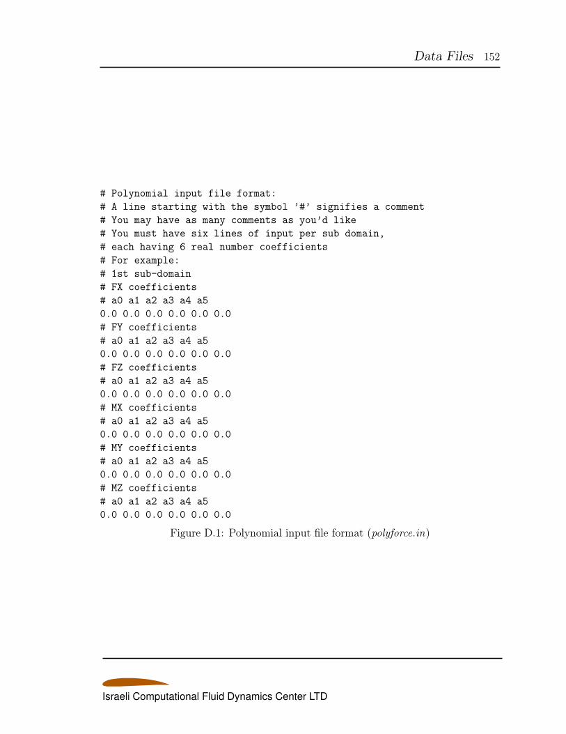
Data Files 152
# Polynomial input file format:
# A line starting with the symbol ’#’ signifies a comment
# You may have as many comments as you’d like
# You must have six lines of input per sub domain,
# each having 6 real number coefficients
# For example:
# 1st sub-domain
# FX coefficients
# a0 a1 a2 a3 a4 a5
0.0 0.0 0.0 0.0 0.0 0.0
# FY coefficients
# a0 a1 a2 a3 a4 a5
0.0 0.0 0.0 0.0 0.0 0.0
# FZ coefficients
# a0 a1 a2 a3 a4 a5
0.0 0.0 0.0 0.0 0.0 0.0
# MX coefficients
# a0 a1 a2 a3 a4 a5
0.0 0.0 0.0 0.0 0.0 0.0
# MY coefficients
# a0 a1 a2 a3 a4 a5
0.0 0.0 0.0 0.0 0.0 0.0
# MZ coefficients
# a0 a1 a2 a3 a4 a5
0.0 0.0 0.0 0.0 0.0 0.0
Figure D.1: Polynomial input file format (polyforce.in)
Israeli Computational Fluid Dynamics Center LTD
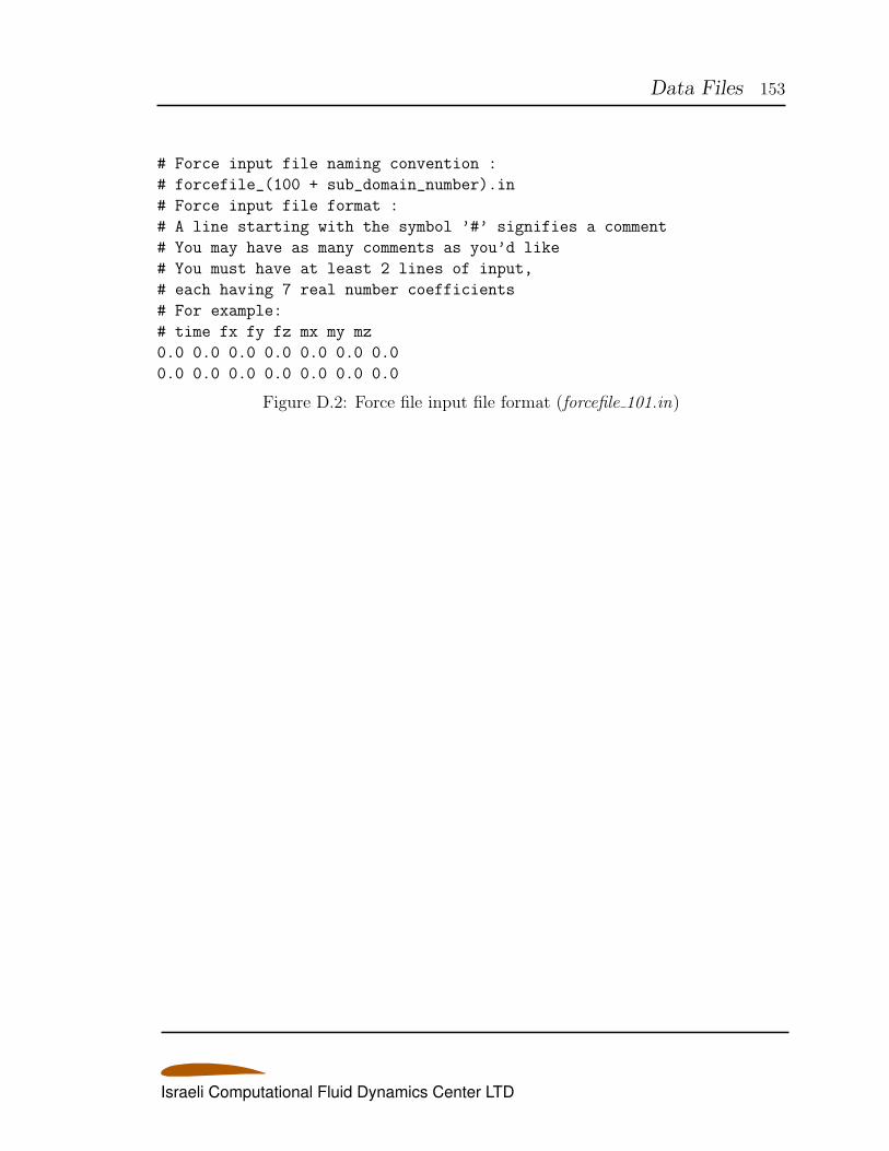
Data Files 153
# Force input file naming convention :
# forcefile_(100 + sub_domain_number).in
# Force input file format :
# A line starting with the symbol ’#’ signifies a comment
# You may have as many comments as you’d like
# You must have at least 2 lines of input,
# each having 7 real number coefficients
# For example:
# time fx fy fz mx my mz
0.0 0.0 0.0 0.0 0.0 0.0 0.0
0.0 0.0 0.0 0.0 0.0 0.0 0.0
Figure D.2: Force file input file format (forcefile 101.in)
Israeli Computational Fluid Dynamics Center LTD
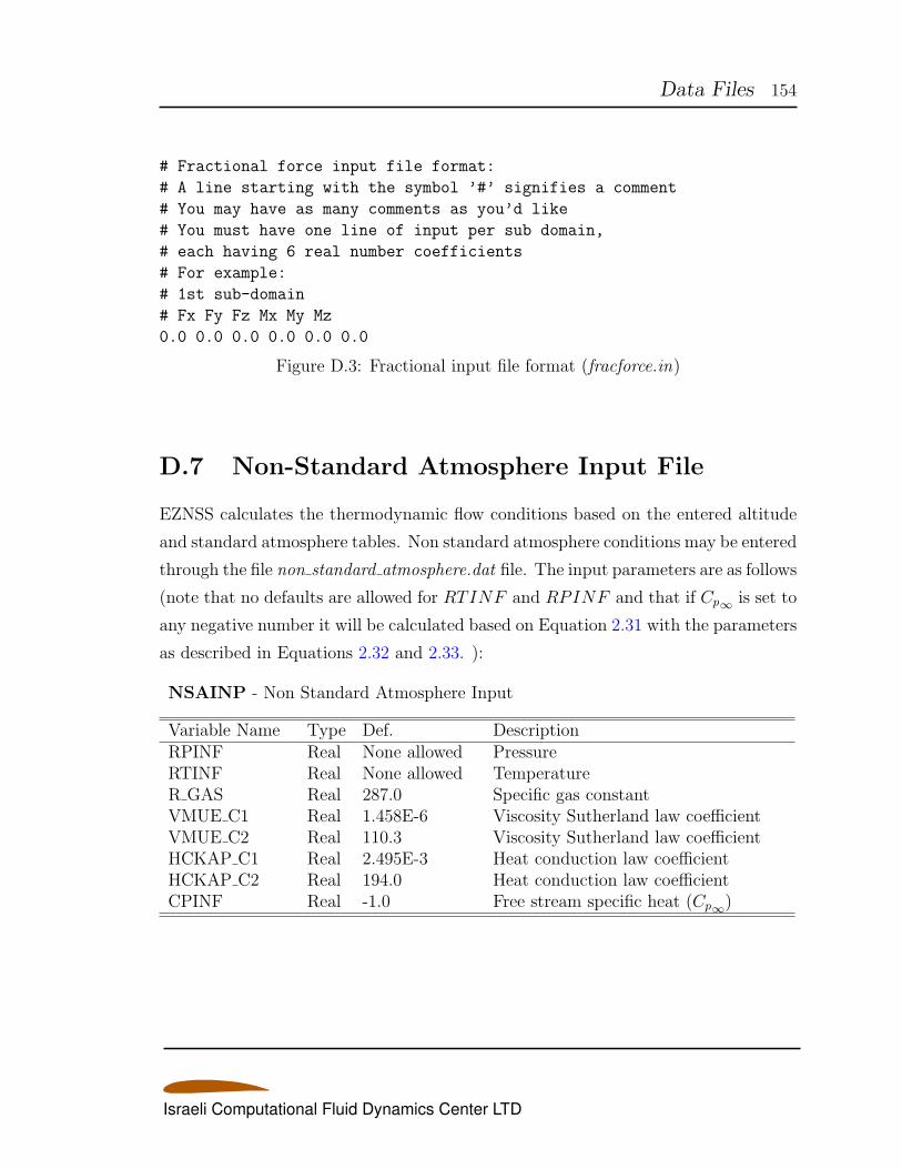
Data Files 154
# Fractional force input file format:
# A line starting with the symbol ’#’ signifies a comment
# You may have as many comments as you’d like
# You must have one line of input per sub domain,
# each having 6 real number coefficients
# For example:
# 1st sub-domain
# Fx Fy Fz Mx My Mz
0.0 0.0 0.0 0.0 0.0 0.0
Figure D.3: Fractional input file format (fracforce.in)
D.7 Non-Standard Atmosphere Input File
EZNSS calculates the thermodynamic flow conditions based on the entered altitude
and standard atmosphere tables. Non standard atmosphere conditions may be entered
through the file non standard atmosphere.dat file. The input parameters are as follows
(note that no defaults are allowed for RTINF and RPINF and that if Cp∞ is set to
any negative number it will be calculated based on Equation 2.31 with the parameters
as described in Equations 2.32 and 2.33. ):
NSAINP - Non Standard Atmosphere Input
Variable Name Type Def. DescriptionRPINF Real None allowed PressureRTINF Real None allowed TemperatureR GAS Real 287.0 Specific gas constantVMUE C1 Real 1.458E-6 Viscosity Sutherland law coefficientVMUE C2 Real 110.3 Viscosity Sutherland law coefficientHCKAP C1 Real 2.495E-3 Heat conduction law coefficientHCKAP C2 Real 194.0 Heat conduction law coefficientCPINF Real -1.0 Free stream specific heat (Cp∞)
Israeli Computational Fluid Dynamics Center LTD
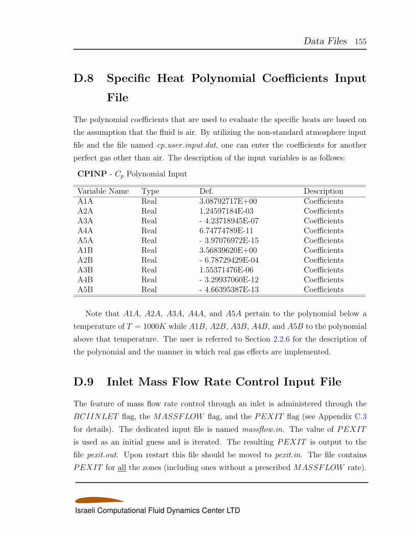
Data Files 155
D.8 Specific Heat Polynomial Coefficients Input
File
The polynomial coefficients that are used to evaluate the specific heats are based on
the assumption that the fluid is air. By utilizing the non-standard atmosphere input
file and the file named cp user input.dat, one can enter the coefficients for another
perfect gas other than air. The description of the input variables is as follows:
CPINP - Cp Polynomial Input
Variable Name Type Def. DescriptionA1A Real 3.08792717E+00 CoefficientsA2A Real 1.24597184E-03 CoefficientsA3A Real - 4.23718945E-07 CoefficientsA4A Real 6.74774789E-11 CoefficientsA5A Real - 3.97076972E-15 CoefficientsA1B Real 3.56839620E+00 CoefficientsA2B Real - 6.78729429E-04 CoefficientsA3B Real 1.55371476E-06 CoefficientsA4B Real - 3.29937060E-12 CoefficientsA5B Real - 4.66395387E-13 Coefficients
Note that A1A, A2A, A3A, A4A, and A5A pertain to the polynomial below a
temperature of T = 1000K while A1B, A2B, A3B, A4B, and A5B to the polynomial
above that temperature. The user is referred to Section 2.2.6 for the description of
the polynomial and the manner in which real gas effects are implemented.
D.9 Inlet Mass Flow Rate Control Input File
The feature of mass flow rate control through an inlet is administered through the
BCIINLET flag, the MASSFLOW flag, and the PEXIT flag (see Appendix C.3
for details). The dedicated input file is named massflow.in. The value of PEXIT
is used as an initial guess and is iterated. The resulting PEXIT is output to the
file pexit.out. Upon restart this file should be moved to pexit.in. The file contains
PEXIT for all the zones (including ones without a prescribed MASSFLOW rate).
Israeli Computational Fluid Dynamics Center LTD
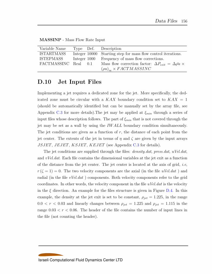
Data Files 156
MASSINP - Mass Flow Rate Input
Variable Name Type Def. DescriptionISTARTMASS Integer 10000 Starting step for mass flow control iterations.ISTEPMASS Integer 1000 Frequency of mass flow corrections.FACTMASSINC Real 0.1 Mass flow correction factor: ∆Pexit = ∆ρu ×
(ρu)∞ × FACTMASSINC
D.10 Jet Input Files
Implementing a jet requires a dedicated zone for the jet. More specifically, the ded-
icated zone must be circular with a KAX boundary condition set to KAX = 1
(should be automatically identified but can be manually set by the array file, see
Appendix C.3 for more details).The jet may be applied at ξmin through a series of
input files whose description follows. The part of ξmin that is not covered through the
jet may be set as a wall by using the IWALL boundary condition simultaneously.
The jet conditions are given as a function of r, the distance of each point from the
jet center. The extents of the jet in terms of η and ζ are given by the input arrays
JSJET , JEJET , KSJET , KEJET (see Appendix C.3 for details).
The jet conditions are supplied through the files: density.dat, press.dat, uVel.dat,
and vVel.dat. Each file contains the dimensional variables at the jet exit as a function
of the distance from the jet center. The jet center is located at the axis of grid, i.e,
r (ζ = 1) = 0. The two velocity components are the axial (in the file uVel.dat ) and
radial (in the file vVel.dat ) components. Both velocity components refer to the grid
coordinates. In other words, the velocity component in the file uVel.dat is the velocity
in the ξ direction. An example for the files structure is given in Figure D.4. In this
example, the density at the jet exit is set to be constant, ρjet = 1.225, in the range
0.0 < r < 0.03 and linearly changes between ρjet = 1.225 and ρjet = 1.115 in the
range 0.03 < r < 0.06. The header of the file contains the number of input lines in
the file (not counting the header).
Israeli Computational Fluid Dynamics Center LTD
Data Files 157
3
0.0 1.225
0.03 1.225
0.06 1.115
Figure D.4: An example of a typical input file (density.dat)
D.11 Discrete Force Input Files
Discrete forces acting on certain surface panels can be modeled using the discrete
force feature. The location of the force is prescribed in the main input file. The
actual force itself is prescribed a series of input files named: discreteforcefile [100 +
force number].in.
# Point force input file naming convention :
# pointforcefile_(100 + point_force_file_number).in
# Point force input file format :
# A line starting with the symbol ’#’ signifies a comment
# You may have as many comments as you’d like
# You must have at least 2 lines of input each having 2 real numbers.
# One for the time and second for the discrete force
# For example:
# time discrete_force
0.0 0.0
0.0 0.0
Figure D.5: Discrete force input file format (discreteforcefile [100 + force number].in)
Each of the discrete forces may be associated to a sub-domain using the array
I DF SUB DOMAIN (see description of the main input file in Section C.2). If
the discrete force is associated to a sub-domain it acts us an injection force (and
moment when applicable). It preempts the ejection force moment and stroke that are
prescribed in the 6dof.i file
Israeli Computational Fluid Dynamics Center LTD
Data Files 158
D.12 Sectional Force and Moment Output
Forces and moment calculation for each zone are reported in the file series fort.7???
and each sub-domain forces and moments are reported in the file series fort.8??? or
fort.9??? (in body coordinates). In addition, the user may supply a list of sections
for which forces and moments are calculated. This is prescribed in the file surface -
force list.dat. The structure of the file is as follows:
1
1 1 1 1 1 1 1
Figure D.6: File format for (surface force list.dat)
The first line signifies the number of entries. Each entry contains seven integer
values signifying the zone number of the section followed by ξmin, ξmax, ηmin, ηmax,
ζmin, ζmax. The results are reported in a list of files, one per entry, with the naming
convention: surface force [100+entry number].dat for the forces and moments and
surface force coeffs [100+entry number].dat for the coefficients. Each line contains
the step number, the time, and six values for the forces and moments or the coefficients
thereof.
Israeli Computational Fluid Dynamics Center LTD
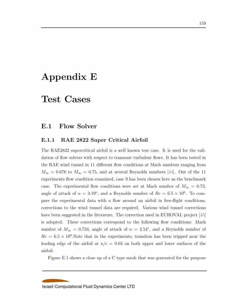
159
Appendix E
Test Cases
E.1 Flow Solver
E.1.1 RAE 2822 Super Critical Airfoil
The RAE2822 supercritical airfoil is a well known test case. It is used for the vali-
dation of flow solvers with respect to transonic turbulent flows. It has been tested in
the RAE wind tunnel in 11 different flow conditions at Mach numbers ranging from
M∞ = 0.676 to M∞ = 0.75, and at several Reynolds numbers [44]. Out of the 11
experiments flow condition examined, case 9 has been chosen here as the benchmark
case. The experimental flow conditions were set at Mach number of M∞ = 0.73,
angle of attack of α = 3.19, and a Reynolds number of Re = 6.5 × 10⁶. To com-
pare the experimental data with a flow around an airfoil in free-flight conditions,
corrections to the wind tunnel data are required. Various wind tunnel corrections
have been suggested in the literature. The correction used in EUROVAL project [45]
is adopted. These corrections correspond to the following flow conditions: Mach
number of M∞ = 0.734, angle of attack of α = 2.54, and a Reynolds number of
Re = 6.5 × 10⁶.Note that in the experiments, transiton has been tripped near the
leading edge of the airfoil at x/c = 0.03 on both upper and lower surfaces of the
airfoil.
Figure E.1 shows a close up of a C type mesh that was generated for the purpose
Israeli Computational Fluid Dynamics Center LTD
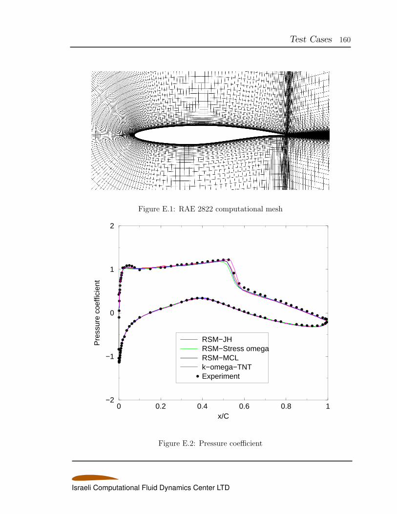
Test Cases 160
Figure E.1: RAE 2822 computational mesh
0 0.2 0.4 0.6 0.8 1x/C
−2
−1
0
1
2
Pre
ssur
e co
effic
ient
RSM−JHRSM−Stress omegaRSM−MCLk−omega−TNTExperiment
Figure E.2: Pressure coefficient
Israeli Computational Fluid Dynamics Center LTD
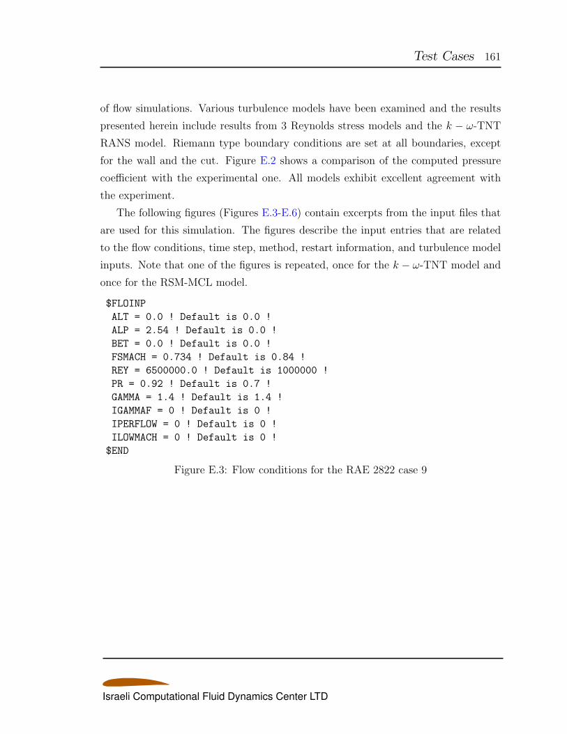
Test Cases 161
of flow simulations. Various turbulence models have been examined and the results
presented herein include results from 3 Reynolds stress models and the k − ω-TNT
RANS model. Riemann type boundary conditions are set at all boundaries, except
for the wall and the cut. Figure E.2 shows a comparison of the computed pressure
coefficient with the experimental one. All models exhibit excellent agreement with
the experiment.
The following figures (Figures E.3-E.6) contain excerpts from the input files that
are used for this simulation. The figures describe the input entries that are related
to the flow conditions, time step, method, restart information, and turbulence model
inputs. Note that one of the figures is repeated, once for the k − ω-TNT model and
once for the RSM-MCL model.
$FLOINP
ALT = 0.0 ! Default is 0.0 !
ALP = 2.54 ! Default is 0.0 !
BET = 0.0 ! Default is 0.0 !
FSMACH = 0.734 ! Default is 0.84 !
REY = 6500000.0 ! Default is 1000000 !
PR = 0.92 ! Default is 0.7 !
GAMMA = 1.4 ! Default is 1.4 !
IGAMMAF = 0 ! Default is 0 !
IPERFLOW = 0 ! Default is 0 !
ILOWMACH = 0 ! Default is 0 !
$END
Figure E.3: Flow conditions for the RAE 2822 case 9
Israeli Computational Fluid Dynamics Center LTD
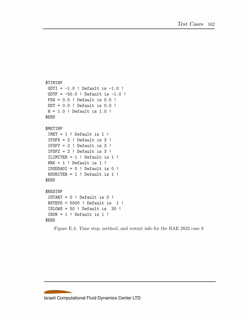
Test Cases 162
$TIMINP
GDTI = -1.0 ! Default is -1.0 !
GDTF = -50.0 ! Default is -1.0 !
FSA = 0.5 ! Default is 0.5 !
DDT = 0.0 ! Default is 0.0 !
H = 1.0 ! Default is 1.0 !
$END
$METINP
IMET = 1 ! Default is 1 !
IFSFX = 2 ! Default is 3 !
IFSFY = 2 ! Default is 3 !
IFSFZ = 2 ! Default is 3 !
ILIMITER = 1 ! Default is 1 !
NRK = 1 ! Default is 1 !
IDODDADI = 0 ! Default is 0 !
NSUBITER = 1 ! Default is 1 !
$END
$RESINP
ISTART = 0 ! Default is 0 !
NSTEPS = 5000 ! Default is 1 !
ISLOWS = 50 ! Default is 30 !
IRUN = 1 ! Default is 1 !
$END
Figure E.4: Time step, method, and restart info for the RAE 2822 case 9
Israeli Computational Fluid Dynamics Center LTD
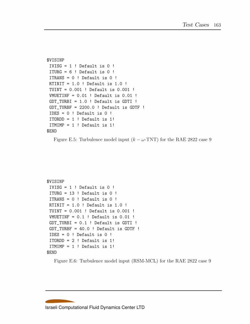
Test Cases 163
$VISINP
IVISG = 1 ! Default is 0 !
ITURG = 6 ! Default is 0 !
ITRANS = 0 ! Default is 0 !
RTINIT = 1.0 ! Default is 1.0 !
TUINT = 0.001 ! Default is 0.001 !
VMUETINF = 0.01 ! Default is 0.01 !
GDT_TURBI = 1.0 ! Default is GDTI !
GDT_TURBF = 2200.0 ! Default is GDTF !
IDES = 0 ! Default is 0 !
ITORDD = 1 ! Default is 1!
ITMIMP = 1 ! Default is 1!
$END
Figure E.5: Turbulence model input (k − ω-TNT) for the RAE 2822 case 9
$VISINP
IVISG = 1 ! Default is 0 !
ITURG = 13 ! Default is 0 !
ITRANS = 0 ! Default is 0 !
RTINIT = 1.0 ! Default is 1.0 !
TUINT = 0.001 ! Default is 0.001 !
VMUETINF = 0.1 ! Default is 0.01 !
GDT_TURBI = 0.1 ! Default is GDTI !
GDT_TURBF = 40.0 ! Default is GDTF !
IDES = 0 ! Default is 0 !
ITORDD = 2 ! Default is 1!
ITMIMP = 1 ! Default is 1!
$END
Figure E.6: Turbulence model input (RSM-MCL) for the RAE 2822 case 9
Israeli Computational Fluid Dynamics Center LTD
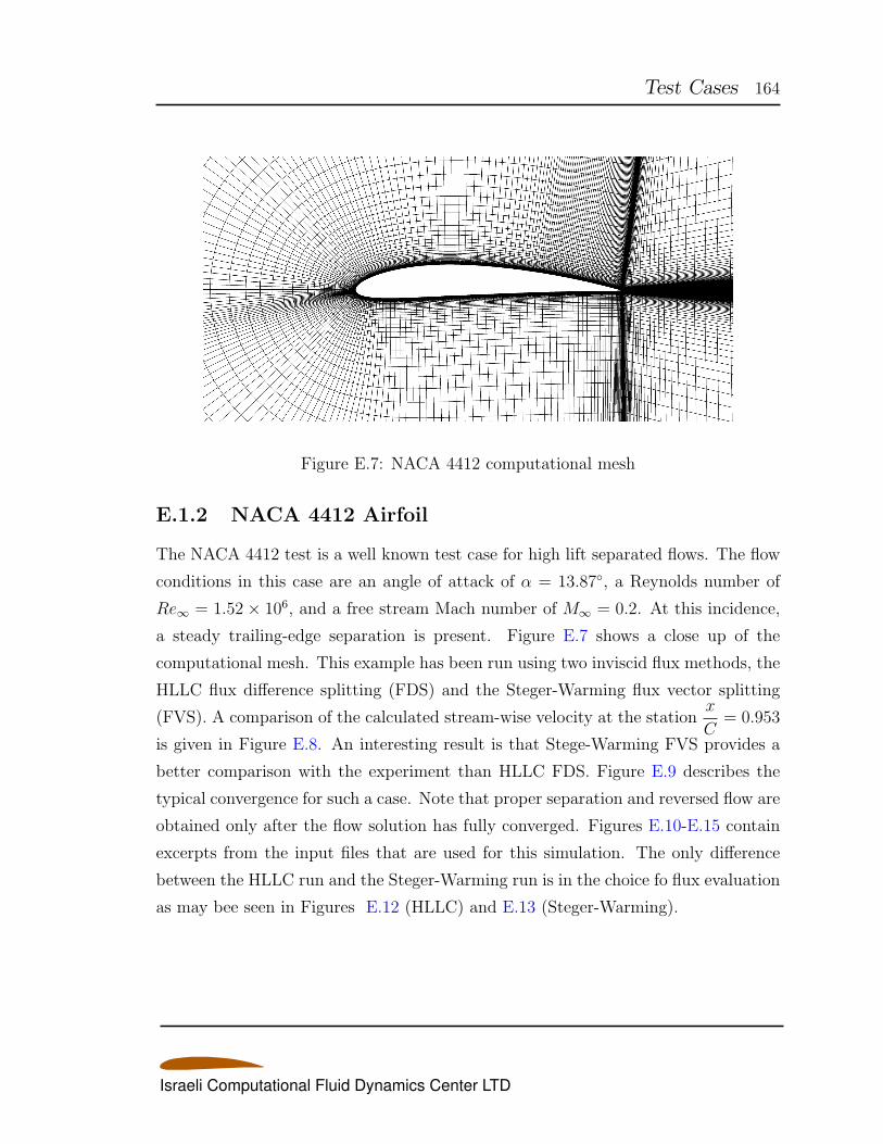
Test Cases 164
Figure E.7: NACA 4412 computational mesh
E.1.2 NACA 4412 Airfoil
The NACA 4412 test is a well known test case for high lift separated flows. The flow
conditions in this case are an angle of attack of α = 13.87, a Reynolds number of
Re∞ = 1.52× 10⁶, and a free stream Mach number of M∞ = 0.2. At this incidence,
a steady trailing-edge separation is present. Figure E.7 shows a close up of the
computational mesh. This example has been run using two inviscid flux methods, the
HLLC flux difference splitting (FDS) and the Steger-Warming flux vector splitting
(FVS). A comparison of the calculated stream-wise velocity at the stationx
C= 0.953
is given in Figure E.8. An interesting result is that Stege-Warming FVS provides a
better comparison with the experiment than HLLC FDS. Figure E.9 describes the
typical convergence for such a case. Note that proper separation and reversed flow are
obtained only after the flow solution has fully converged. Figures E.10-E.15 contain
excerpts from the input files that are used for this simulation. The only difference
between the HLLC run and the Steger-Warming run is in the choice fo flux evaluation
as may bee seen in Figures E.12 (HLLC) and E.13 (Steger-Warming).
Israeli Computational Fluid Dynamics Center LTD
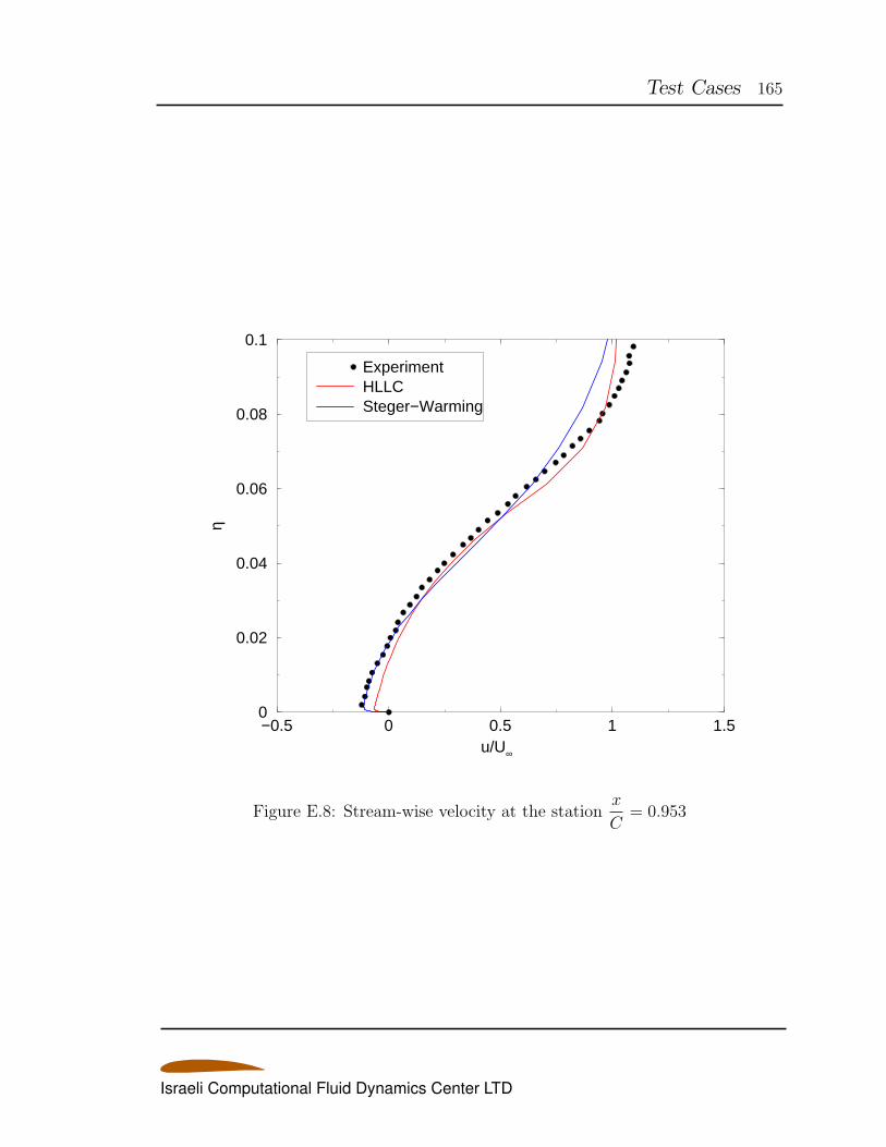
Test Cases 165
−0.5 0 0.5 1 1.5u/U∞
0
0.02
0.04
0.06
0.08
0.1
η
ExperimentHLLCSteger−Warming
Figure E.8: Stream-wise velocity at the stationx
C= 0.953
Israeli Computational Fluid Dynamics Center LTD
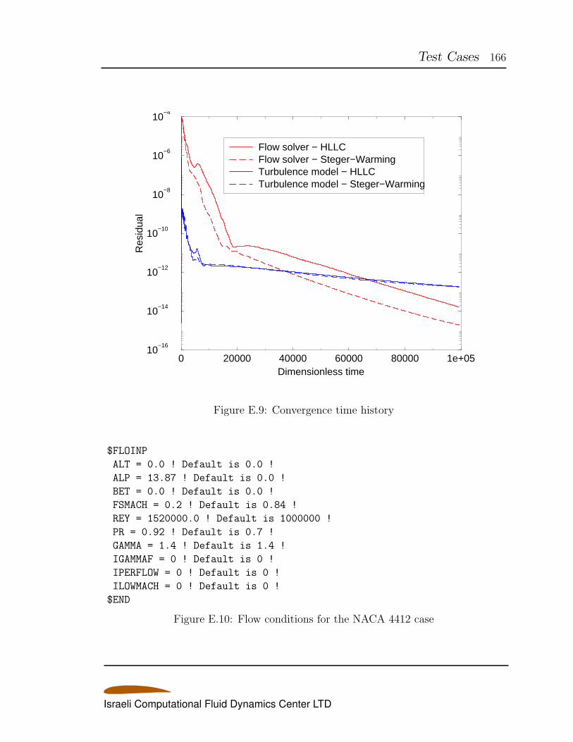
Test Cases 166
0 20000 40000 60000 80000 1e+05Dimensionless time
10−16
10−14
10−12
10−10
10−8
10−6
10−4
Res
idua
lFlow solver − HLLCFlow solver − Steger−WarmingTurbulence model − HLLCTurbulence model − Steger−Warming
Figure E.9: Convergence time history
$FLOINP
ALT = 0.0 ! Default is 0.0 !
ALP = 13.87 ! Default is 0.0 !
BET = 0.0 ! Default is 0.0 !
FSMACH = 0.2 ! Default is 0.84 !
REY = 1520000.0 ! Default is 1000000 !
PR = 0.92 ! Default is 0.7 !
GAMMA = 1.4 ! Default is 1.4 !
IGAMMAF = 0 ! Default is 0 !
IPERFLOW = 0 ! Default is 0 !
ILOWMACH = 0 ! Default is 0 !
$END
Figure E.10: Flow conditions for the NACA 4412 case
Israeli Computational Fluid Dynamics Center LTD
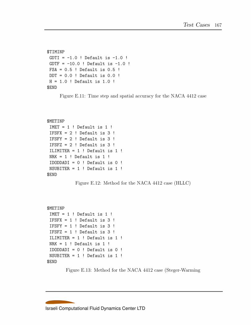
Test Cases 167
$TIMINP
GDTI = -1.0 ! Default is -1.0 !
GDTF = -10.0 ! Default is -1.0 !
FSA = 0.5 ! Default is 0.5 !
DDT = 0.0 ! Default is 0.0 !
H = 1.0 ! Default is 1.0 !
$END
Figure E.11: Time step and spatial accuracy for the NACA 4412 case
$METINP
IMET = 1 ! Default is 1 !
IFSFX = 2 ! Default is 3 !
IFSFY = 2 ! Default is 3 !
IFSFZ = 2 ! Default is 3 !
ILIMITER = 1 ! Default is 1 !
NRK = 1 ! Default is 1 !
IDODDADI = 0 ! Default is 0 !
NSUBITER = 1 ! Default is 1 !
$END
Figure E.12: Method for the NACA 4412 case (HLLC)
$METINP
IMET = 1 ! Default is 1 !
IFSFX = 1 ! Default is 3 !
IFSFY = 1 ! Default is 3 !
IFSFZ = 1 ! Default is 3 !
ILIMITER = 1 ! Default is 1 !
NRK = 1 ! Default is 1 !
IDODDADI = 0 ! Default is 0 !
NSUBITER = 1 ! Default is 1 !
$END
Figure E.13: Method for the NACA 4412 case (Steger-Warming
Israeli Computational Fluid Dynamics Center LTD
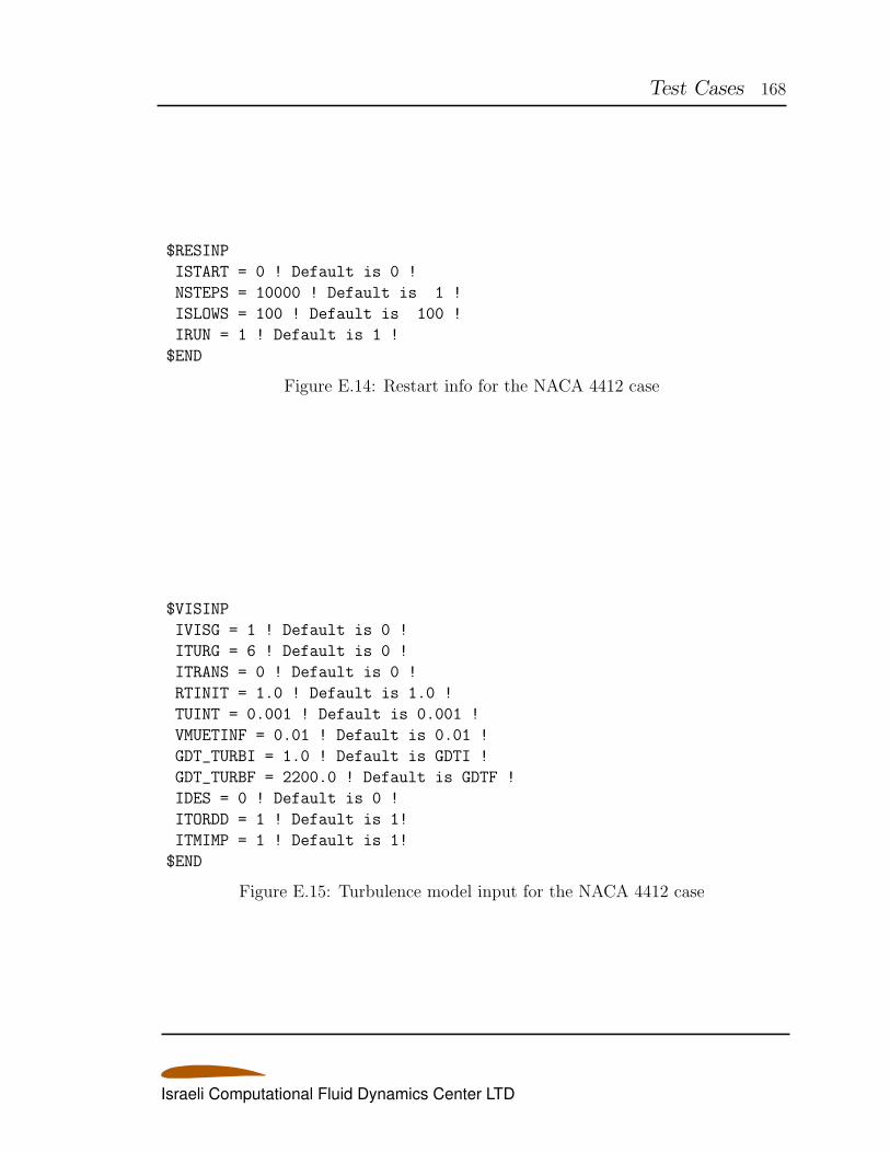
Test Cases 168
$RESINP
ISTART = 0 ! Default is 0 !
NSTEPS = 10000 ! Default is 1 !
ISLOWS = 100 ! Default is 100 !
IRUN = 1 ! Default is 1 !
$END
Figure E.14: Restart info for the NACA 4412 case
$VISINP
IVISG = 1 ! Default is 0 !
ITURG = 6 ! Default is 0 !
ITRANS = 0 ! Default is 0 !
RTINIT = 1.0 ! Default is 1.0 !
TUINT = 0.001 ! Default is 0.001 !
VMUETINF = 0.01 ! Default is 0.01 !
GDT_TURBI = 1.0 ! Default is GDTI !
GDT_TURBF = 2200.0 ! Default is GDTF !
IDES = 0 ! Default is 0 !
ITORDD = 1 ! Default is 1!
ITMIMP = 1 ! Default is 1!
$END
Figure E.15: Turbulence model input for the NACA 4412 case
Israeli Computational Fluid Dynamics Center LTD
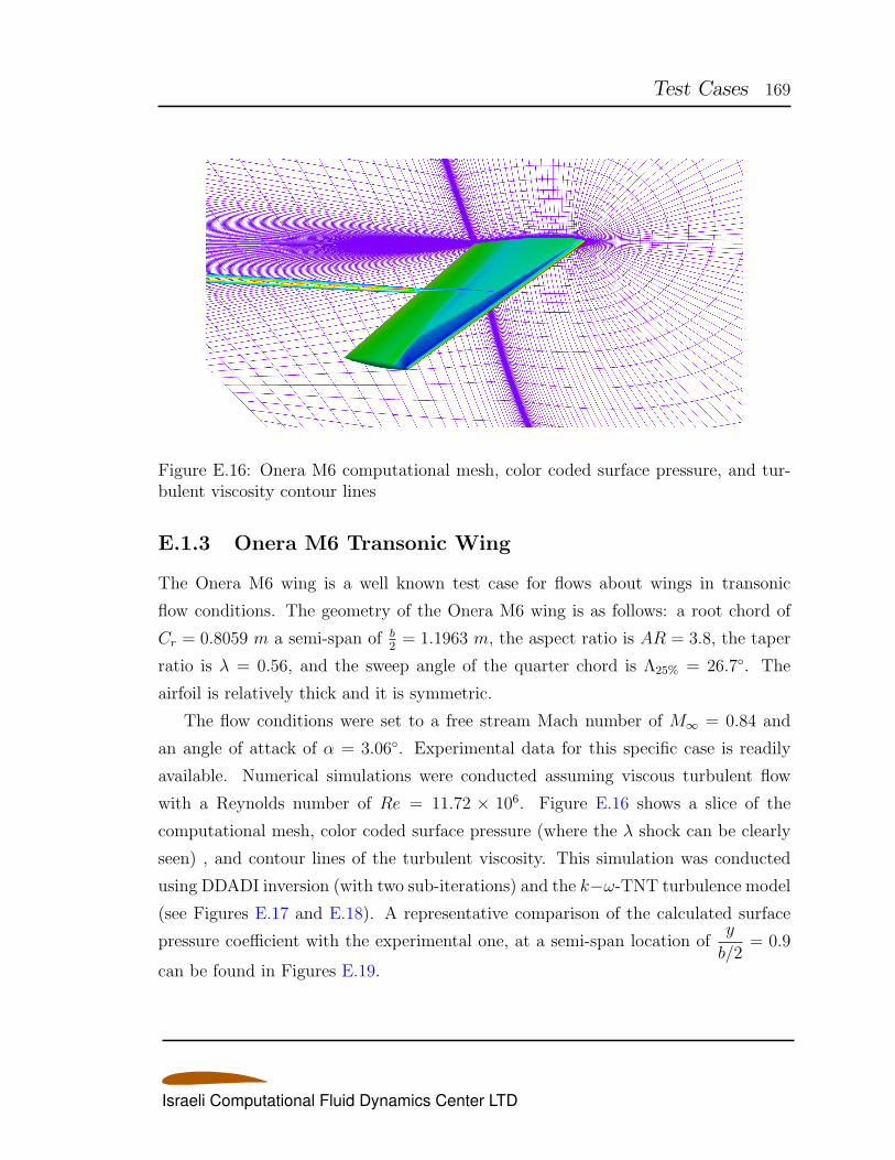
Test Cases 169
Figure E.16: Onera M6 computational mesh, color coded surface pressure, and tur-bulent viscosity contour lines
E.1.3 Onera M6 Transonic Wing
The Onera M6 wing is a well known test case for flows about wings in transonic
flow conditions. The geometry of the Onera M6 wing is as follows: a root chord of
Cr = 0.8059 m a semi-span of b2= 1.1963 m, the aspect ratio is AR = 3.8, the taper
ratio is λ = 0.56, and the sweep angle of the quarter chord is Λ25% = 26.7. The
airfoil is relatively thick and it is symmetric.
The flow conditions were set to a free stream Mach number of M∞ = 0.84 and
an angle of attack of α = 3.06. Experimental data for this specific case is readily
available. Numerical simulations were conducted assuming viscous turbulent flow
with a Reynolds number of Re = 11.72 × 10⁶. Figure E.16 shows a slice of the
computational mesh, color coded surface pressure (where the λ shock can be clearly
seen) , and contour lines of the turbulent viscosity. This simulation was conducted
using DDADI inversion (with two sub-iterations) and the k−ω-TNT turbulence model
(see Figures E.17 and E.18). A representative comparison of the calculated surface
pressure coefficient with the experimental one, at a semi-span location ofy
b/2= 0.9
can be found in Figures E.19.
Israeli Computational Fluid Dynamics Center LTD
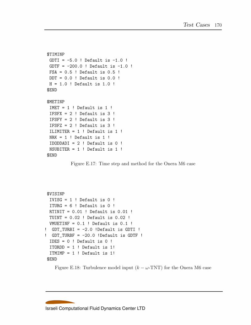
Test Cases 170
$TIMINP
GDTI = -5.0 ! Default is -1.0 !
GDTF = -200.0 ! Default is -1.0 !
FSA = 0.5 ! Default is 0.5 !
DDT = 0.0 ! Default is 0.0 !
H = 1.0 ! Default is 1.0 !
$END
$METINP
IMET = 1 ! Default is 1 !
IFSFX = 2 ! Default is 3 !
IFSFY = 2 ! Default is 3 !
IFSFZ = 2 ! Default is 3 !
ILIMITER = 1 ! Default is 1 !
NRK = 1 ! Default is 1 !
IDODDADI = 2 ! Default is 0 !
NSUBITER = 1 ! Default is 1 !
$END
Figure E.17: Time step and method for the Onera M6 case
$VISINP
IVISG = 1 ! Default is 0 !
ITURG = 6 ! Default is 0 !
RTINIT = 0.01 ! Default is 0.01 !
TUINT = 0.02 ! Default is 0.02 !
VMUETINF = 0.1 ! Default is 0.1 !
! GDT_TURBI = -2.0 !Default is GDTI !
! GDT_TURBF = -20.0 !Default is GDTF !
IDES = 0 ! Default is 0 !
ITORDD = 1 ! Default is 1!
ITMIMP = 1 ! Default is 1!
$END
Figure E.18: Turbulence model input (k − ω-TNT) for the Onera M6 case
Israeli Computational Fluid Dynamics Center LTD
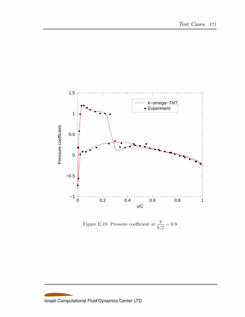
Test Cases 171
0 0.2 0.4 0.6 0.8 1x/C
−1
−0.5
0
0.5
1
1.5
Pre
ssur
e co
effic
ient
k−omega−TNTExperiment
Figure E.19: Pressure coefficient aty
b/2= 0.9
Israeli Computational Fluid Dynamics Center LTD
Test Cases 172
E.2 Aeroelasticity Module
E.2.1 Basic Wing-Fuselage-Tail Test-Case - The PHDP
The basic test case is that of a generic transport model (a.k.a. PhD plane, or PHDP)
that includes thre aerodynamic grid zones for the fuselage, wing and tail, plus collar
zones. The structural grids are provided in three separate files, grid s 101.dat, grid -
s 102.dat, and grid s 103.dat, for the fuselage, wing and tail respectively. Figure E.20
presents a sample grid file structure. The modes are provided in NASTRAN punch
format, in files mode s 101.dat, mode s 102.dat, and mode s 103.dat, for the fuselage,
wing and tail respectively. Figure E.21 presents a sample modes-file structure. Each
mode file has 15 modes, out of which two are rigid-body modes. The first five modes
are splined to the aerodynamic surface grids (N MODES=5), and out of them only
the first three elastic modes are used in the aeroelastic analysis. The two rigid body
modes (N RBMODES = 2) are splined to the aero grids but are not used in the
aeroelastic analysis.
Figures E.22 and E.23 present the elastic- and spline-related inputs, respectively,
in the main input file eznss.i.defaults. In this run IELAST = -1, namely the code
performs the spline and exists (no aerodynamic/aeroelastic analysis is performed).
The rest of the parameters in the ELAINP namelist are therefore irrelevant for this
analysis. Figure E.24 presents the first two entries in file spline.i for this test case,
indicating that the first structural zone (fuselage) goes through beam spline (IS -
SS=0), while the second and third structural zones (wing and tail) go through surface
spline (IS SS=1), and that aerodynamic zone number 1 gets its spline info from
structural zone number 1 (ISPLINE FROM = 1), and similarly 2 from 2 and 3 from
3. The rest of the entries in file spline.i get their default values.
Figure E.25 presents the wing surface mesh (grey, only every other i grid), and on
top of it the structural nodes that are used in the wing mode spline (red, connected
in line). The structural data is from file struct 100.dat. Plotting the structural
spline nodes on top of the aerodynamic surfaces serves for validation of the selected
structural spline nodes. Figure E.26 presents the first elastic mode, plotted from file
mode a 103.dat (blue), together with the undeformed surface grids (grey). Similar
Israeli Computational Fluid Dynamics Center LTD
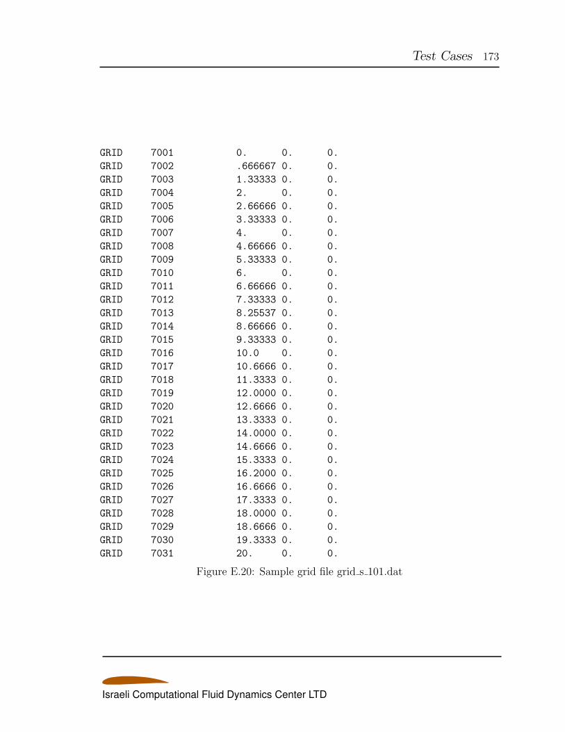
Test Cases 173
GRID 7001 0. 0. 0.
GRID 7002 .666667 0. 0.
GRID 7003 1.33333 0. 0.
GRID 7004 2. 0. 0.
GRID 7005 2.66666 0. 0.
GRID 7006 3.33333 0. 0.
GRID 7007 4. 0. 0.
GRID 7008 4.66666 0. 0.
GRID 7009 5.33333 0. 0.
GRID 7010 6. 0. 0.
GRID 7011 6.66666 0. 0.
GRID 7012 7.33333 0. 0.
GRID 7013 8.25537 0. 0.
GRID 7014 8.66666 0. 0.
GRID 7015 9.33333 0. 0.
GRID 7016 10.0 0. 0.
GRID 7017 10.6666 0. 0.
GRID 7018 11.3333 0. 0.
GRID 7019 12.0000 0. 0.
GRID 7020 12.6666 0. 0.
GRID 7021 13.3333 0. 0.
GRID 7022 14.0000 0. 0.
GRID 7023 14.6666 0. 0.
GRID 7024 15.3333 0. 0.
GRID 7025 16.2000 0. 0.
GRID 7026 16.6666 0. 0.
GRID 7027 17.3333 0. 0.
GRID 7028 18.0000 0. 0.
GRID 7029 18.6666 0. 0.
GRID 7030 19.3333 0. 0.
GRID 7031 20. 0. 0.
Figure E.20: Sample grid file grid s 101.dat
Israeli Computational Fluid Dynamics Center LTD
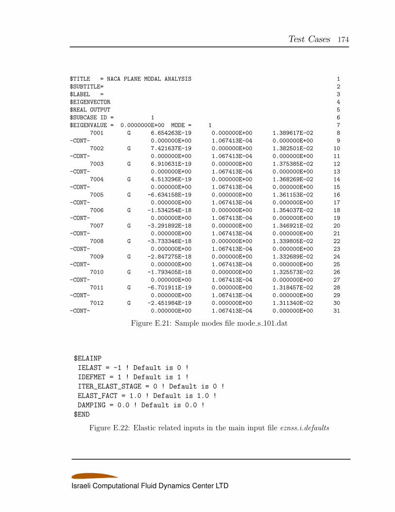
Test Cases 174
$TITLE = NACA PLANE MODAL ANALYSIS 1
$SUBTITLE= 2
$LABEL = 3
$EIGENVECTOR 4
$REAL OUTPUT 5
$SUBCASE ID = 1 6
$EIGENVALUE = 0.0000000E+00 MODE = 1 7
7001 G 6.654263E-19 0.000000E+00 1.389617E-02 8
-CONT- 0.000000E+00 1.067413E-04 0.000000E+00 9
7002 G 7.421637E-19 0.000000E+00 1.382501E-02 10
-CONT- 0.000000E+00 1.067413E-04 0.000000E+00 11
7003 G 6.910631E-19 0.000000E+00 1.375385E-02 12
-CONT- 0.000000E+00 1.067413E-04 0.000000E+00 13
7004 G 4.513296E-19 0.000000E+00 1.368269E-02 14
-CONT- 0.000000E+00 1.067413E-04 0.000000E+00 15
7005 G -6.634158E-19 0.000000E+00 1.361153E-02 16
-CONT- 0.000000E+00 1.067413E-04 0.000000E+00 17
7006 G -1.534254E-18 0.000000E+00 1.354037E-02 18
-CONT- 0.000000E+00 1.067413E-04 0.000000E+00 19
7007 G -3.291892E-18 0.000000E+00 1.346921E-02 20
-CONT- 0.000000E+00 1.067413E-04 0.000000E+00 21
7008 G -3.733346E-18 0.000000E+00 1.339805E-02 22
-CONT- 0.000000E+00 1.067413E-04 0.000000E+00 23
7009 G -2.847275E-18 0.000000E+00 1.332689E-02 24
-CONT- 0.000000E+00 1.067413E-04 0.000000E+00 25
7010 G -1.793405E-18 0.000000E+00 1.325573E-02 26
-CONT- 0.000000E+00 1.067413E-04 0.000000E+00 27
7011 G -6.701911E-19 0.000000E+00 1.318457E-02 28
-CONT- 0.000000E+00 1.067413E-04 0.000000E+00 29
7012 G -2.451984E-19 0.000000E+00 1.311340E-02 30
-CONT- 0.000000E+00 1.067413E-04 0.000000E+00 31
Figure E.21: Sample modes file mode s 101.dat
$ELAINP
IELAST = -1 ! Default is 0 !
IDEFMET = 1 ! Default is 1 !
ITER_ELAST_STAGE = 0 ! Default is 0 !
ELAST_FACT = 1.0 ! Default is 1.0 !
DAMPING = 0.0 ! Default is 0.0 !
$END
Figure E.22: Elastic related inputs in the main input file eznss.i.defaults
Israeli Computational Fluid Dynamics Center LTD
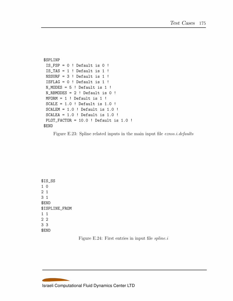
Test Cases 175
$SPLINP
IS_FSP = 0 ! Default is 0 !
IS_TAS = 1 ! Default is 1 !
NSSURF = 3 ! Default is 1 !
ISFLAG = 0 ! Default is 1 !
N_MODES = 5 ! Default is 1 !
N_RBMODES = 2 ! Default is 0 !
MFORM = 1 ! Default is 1 !
SCALE = 1.0 ! Default is 1.0 !
SCALEM = 1.0 ! Default is 1.0 !
SCALEA = 1.0 ! Default is 1.0 !
PLOT_FACTOR = 10.0 ! Default is 1.0 !
$END
Figure E.23: Spline related inputs in the main input file eznss.i.defaults
$IS_SS
1 0
2 1
3 1
$END
$ISPLINE_FROM
1 1
2 2
3 3
$END
Figure E.24: First entries in input file spline.i
Israeli Computational Fluid Dynamics Center LTD
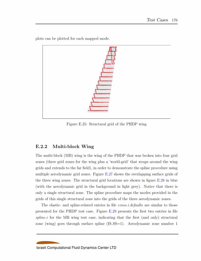
Test Cases 176
plots can be plotted for each mapped mode.
Figure E.25: Structural grid of the PHDP wing
E.2.2 Multi-block Wing
The multi-block (MB) wing is the wing of the PHDP that was broken into four grid
zones (three grid zones for the wing plus a ’world-grid’ that wraps around the wing
grids and extends to the far field), in order to demonstrate the spline procedure using
multiple aerodynamic grid zones. Figure E.27 shows the overlapping surface grids of
the three wing zones. The structural grid locations are shown in figure E.28 in blue
(with the aerodynamic grid in the background in light grey). Notice that there is
only a single structural zone. The spline procedure maps the modes provided in the
grids of this single structural zone into the grids of the three aerodynamic zones.
The elastic- and spline-related entries in file eznss.i.defaults are similar to those
presented for the PHDP test case. Figure E.29 presents the first two entries in file
spline.i for the MB wing test case, indicating that the first (and only) structural
zone (wing) goes through surface spline (IS SS=1). Aerodynamic zone number 1
Israeli Computational Fluid Dynamics Center LTD
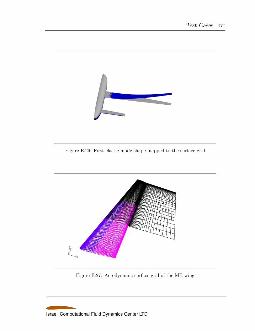
Test Cases 177
Figure E.26: First elastic mode shape mapped to the surface grid
Figure E.27: Aerodynamic surface grid of the MB wing
Israeli Computational Fluid Dynamics Center LTD
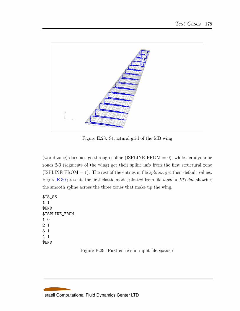
Test Cases 178
Figure E.28: Structural grid of the MB wing
(world zone) does not go through spline (ISPLINE FROM = 0), while aerodynamic
zones 2-3 (segments of the wing) get their spline info from the first structural zone
(ISPLINE FROM = 1). The rest of the entries in file spline.i get their default values.
Figure E.30 presents the first elastic mode, plotted from file mode a 103.dat, showing
the smooth spline across the three zones that make up the wing.
$IS_SS
1 1
$END
$ISPLINE_FROM
1 0
2 1
3 1
4 1
$END
Figure E.29: First entries in input file spline.i
Israeli Computational Fluid Dynamics Center LTD
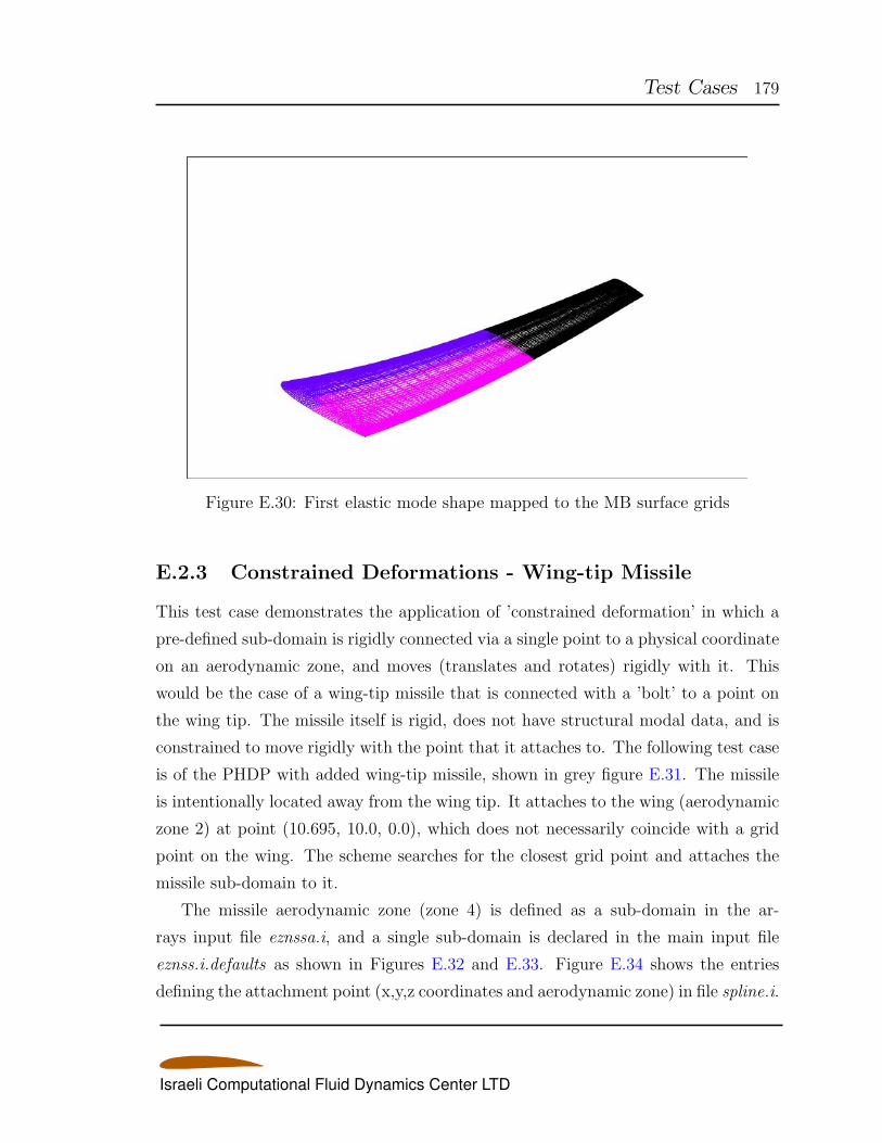
Test Cases 179
Figure E.30: First elastic mode shape mapped to the MB surface grids
E.2.3 Constrained Deformations - Wing-tip Missile
This test case demonstrates the application of ’constrained deformation’ in which a
pre-defined sub-domain is rigidly connected via a single point to a physical coordinate
on an aerodynamic zone, and moves (translates and rotates) rigidly with it. This
would be the case of a wing-tip missile that is connected with a ’bolt’ to a point on
the wing tip. The missile itself is rigid, does not have structural modal data, and is
constrained to move rigidly with the point that it attaches to. The following test case
is of the PHDP with added wing-tip missile, shown in grey figure E.31. The missile
is intentionally located away from the wing tip. It attaches to the wing (aerodynamic
zone 2) at point (10.695, 10.0, 0.0), which does not necessarily coincide with a grid
point on the wing. The scheme searches for the closest grid point and attaches the
missile sub-domain to it.
The missile aerodynamic zone (zone 4) is defined as a sub-domain in the ar-
rays input file eznssa.i, and a single sub-domain is declared in the main input file
eznss.i.defaults as shown in Figures E.32 and E.33. Figure E.34 shows the entries
defining the attachment point (x,y,z coordinates and aerodynamic zone) in file spline.i.
Israeli Computational Fluid Dynamics Center LTD
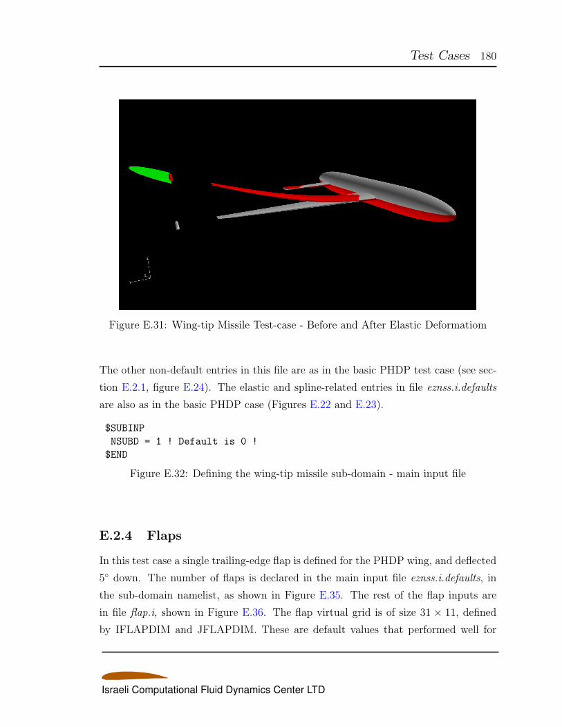
Test Cases 180
Figure E.31: Wing-tip Missile Test-case - Before and After Elastic Deformatiom
The other non-default entries in this file are as in the basic PHDP test case (see sec-
tion E.2.1, figure E.24). The elastic and spline-related entries in file eznss.i.defaults
are also as in the basic PHDP case (Figures E.22 and E.23).
$SUBINP
NSUBD = 1 ! Default is 0 !
$END
Figure E.32: Defining the wing-tip missile sub-domain - main input file
E.2.4 Flaps
In this test case a single trailing-edge flap is defined for the PHDP wing, and deflected
5 down. The number of flaps is declared in the main input file eznss.i.defaults, in
the sub-domain namelist, as shown in Figure E.35. The rest of the flap inputs are
in file flap.i, shown in Figure E.36. The flap virtual grid is of size 31 × 11, defined
by IFLAPDIM and JFLAPDIM. These are default values that performed well for
Israeli Computational Fluid Dynamics Center LTD
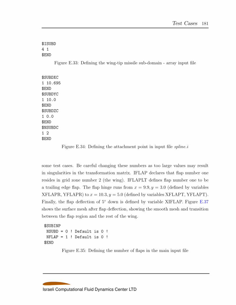
Test Cases 181
$ISUBD
4 1
$END
Figure E.33: Defining the wing-tip missile sub-domain - array input file
$SUBDXC
1 10.695
$END
$SUBDYC
1 10.0
$END
$SUBDZC
1 0.0
$END
$NSUBDC
1 2
$END
Figure E.34: Defining the attachment point in input file spline.i
some test cases. Be careful changing these numbers as too large values may result
in singularities in the transformation matrix. IFLAP declares that flap number one
resides in grid zone number 2 (the wing). IFLAPLT defines flap number one to be
a trailing edge flap. The flap hinge runs from x = 9.9, y = 3.0 (defined by variables
XFLAPR, YFLAPR) to x = 10.3, y = 5.0 (defined by variables XFLAPT, YFLAPT).
Finally, the flap deflection of 5 down is defined by variable XIFLAP. Figure E.37
shows the surface mesh after flap deflection, showing the smooth mesh and transition
between the flap region and the rest of the wing.
$SUBINP
NSUBD = 0 ! Default is 0 !
NFLAP = 1 ! Default is 0 !
$END
Figure E.35: Defining the number of flaps in the main input file
Israeli Computational Fluid Dynamics Center LTD

Test Cases 182
$IFLAPDIM
1 31
$END
$JFLAPDIM
1 11
$END
$IFLAP
1 2
$END
$IFLAPLT
1 1
$END
$XFLAPR
1 9.9
$END
$YFLAPR
1 3.0
$END
$XFLAPT
1 10.3
$END
$YFLAPT
1 5.0
$END
$XIFLAP
1 5.0
$END
Figure E.36: Flap input file
Israeli Computational Fluid Dynamics Center LTD
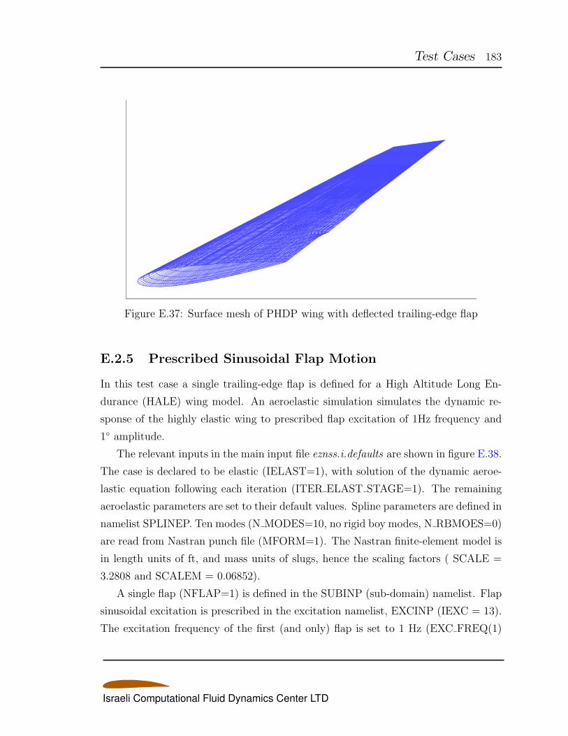
Test Cases 183
Figure E.37: Surface mesh of PHDP wing with deflected trailing-edge flap
E.2.5 Prescribed Sinusoidal Flap Motion
In this test case a single trailing-edge flap is defined for a High Altitude Long En-
durance (HALE) wing model. An aeroelastic simulation simulates the dynamic re-
sponse of the highly elastic wing to prescribed flap excitation of 1Hz frequency and
1 amplitude.
The relevant inputs in the main input file eznss.i.defaults are shown in figure E.38.
The case is declared to be elastic (IELAST=1), with solution of the dynamic aeroe-
lastic equation following each iteration (ITER ELAST STAGE=1). The remaining
aeroelastic parameters are set to their default values. Spline parameters are defined in
namelist SPLINEP. Ten modes (N MODES=10, no rigid boy modes, N RBMOES=0)
are read from Nastran punch file (MFORM=1). The Nastran finite-element model is
in length units of ft, and mass units of slugs, hence the scaling factors ( SCALE =
3.2808 and SCALEM = 0.06852).
A single flap (NFLAP=1) is defined in the SUBINP (sub-domain) namelist. Flap
sinusoidal excitation is prescribed in the excitation namelist, EXCINP (IEXC = 13).
The excitation frequency of the first (and only) flap is set to 1 Hz (EXC FREQ(1)
Israeli Computational Fluid Dynamics Center LTD
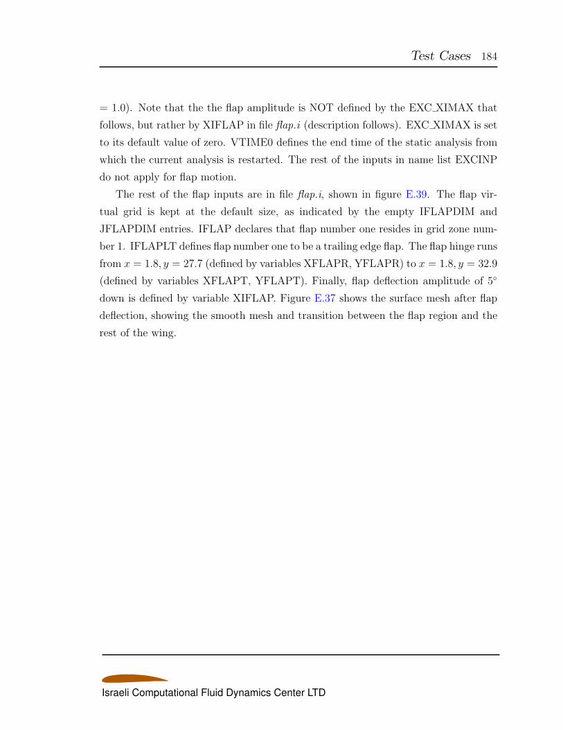
Test Cases 184
= 1.0). Note that the the flap amplitude is NOT defined by the EXC XIMAX that
follows, but rather by XIFLAP in file flap.i (description follows). EXC XIMAX is set
to its default value of zero. VTIME0 defines the end time of the static analysis from
which the current analysis is restarted. The rest of the inputs in name list EXCINP
do not apply for flap motion.
The rest of the flap inputs are in file flap.i, shown in figure E.39. The flap vir-
tual grid is kept at the default size, as indicated by the empty IFLAPDIM and
JFLAPDIM entries. IFLAP declares that flap number one resides in grid zone num-
ber 1. IFLAPLT defines flap number one to be a trailing edge flap. The flap hinge runs
from x = 1.8, y = 27.7 (defined by variables XFLAPR, YFLAPR) to x = 1.8, y = 32.9
(defined by variables XFLAPT, YFLAPT). Finally, flap deflection amplitude of 5
down is defined by variable XIFLAP. Figure E.37 shows the surface mesh after flap
deflection, showing the smooth mesh and transition between the flap region and the
rest of the wing.
Israeli Computational Fluid Dynamics Center LTD
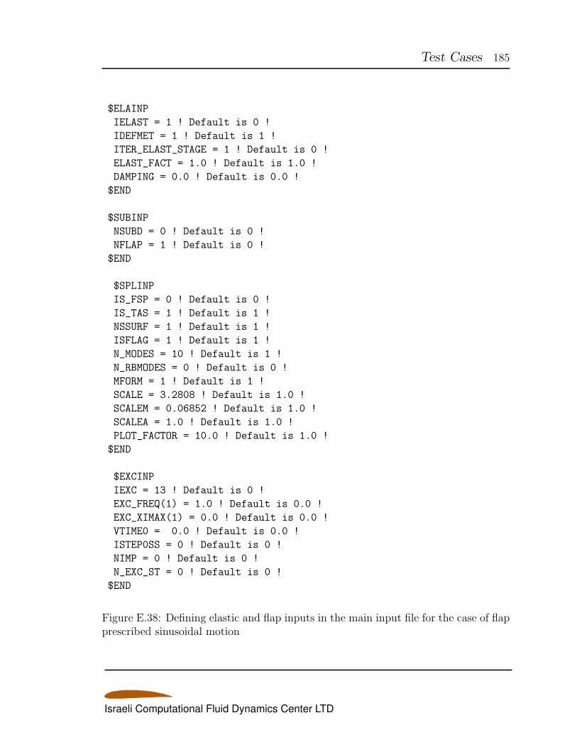
Test Cases 185
$ELAINP
IELAST = 1 ! Default is 0 !
IDEFMET = 1 ! Default is 1 !
ITER_ELAST_STAGE = 1 ! Default is 0 !
ELAST_FACT = 1.0 ! Default is 1.0 !
DAMPING = 0.0 ! Default is 0.0 !
$END
$SUBINP
NSUBD = 0 ! Default is 0 !
NFLAP = 1 ! Default is 0 !
$END
$SPLINP
IS_FSP = 0 ! Default is 0 !
IS_TAS = 1 ! Default is 1 !
NSSURF = 1 ! Default is 1 !
ISFLAG = 1 ! Default is 1 !
N_MODES = 10 ! Default is 1 !
N_RBMODES = 0 ! Default is 0 !
MFORM = 1 ! Default is 1 !
SCALE = 3.2808 ! Default is 1.0 !
SCALEM = 0.06852 ! Default is 1.0 !
SCALEA = 1.0 ! Default is 1.0 !
PLOT_FACTOR = 10.0 ! Default is 1.0 !
$END
$EXCINP
IEXC = 13 ! Default is 0 !
EXC_FREQ(1) = 1.0 ! Default is 0.0 !
EXC_XIMAX(1) = 0.0 ! Default is 0.0 !
VTIME0 = 0.0 ! Default is 0.0 !
ISTEP0SS = 0 ! Default is 0 !
NIMP = 0 ! Default is 0 !
N_EXC_ST = 0 ! Default is 0 !
$END
Figure E.38: Defining elastic and flap inputs in the main input file for the case of flapprescribed sinusoidal motion
Israeli Computational Fluid Dynamics Center LTD
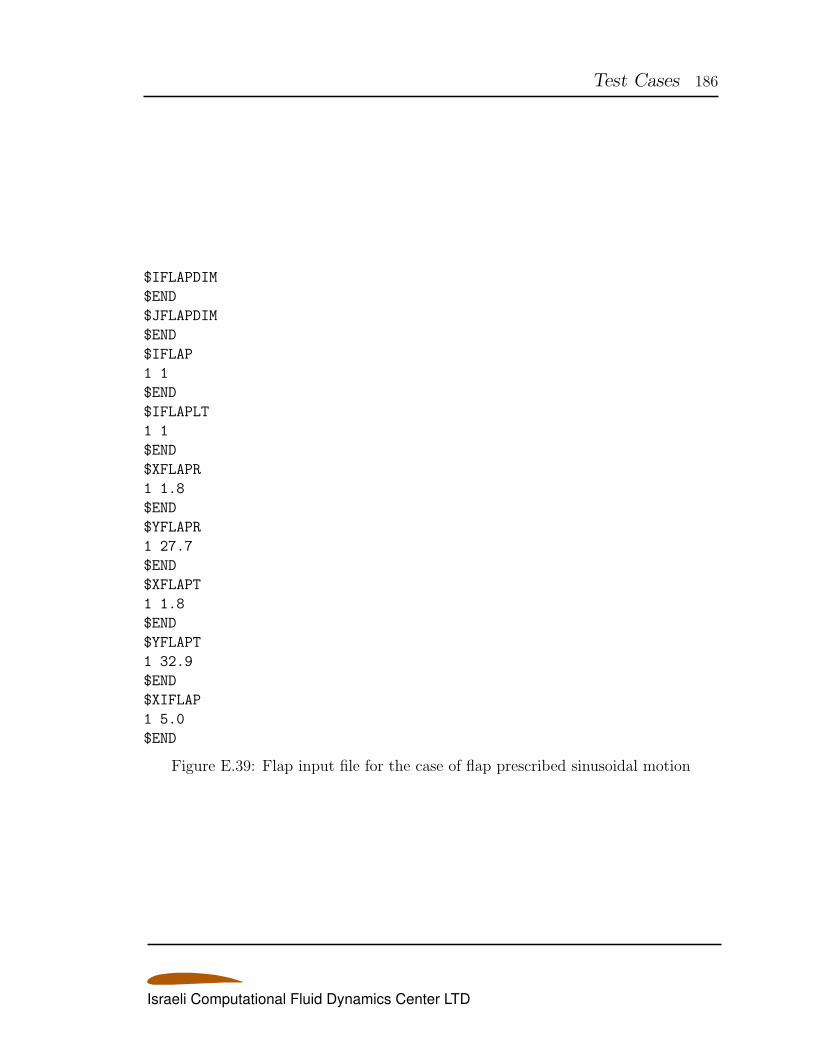
Test Cases 186
$IFLAPDIM
$END
$JFLAPDIM
$END
$IFLAP
1 1
$END
$IFLAPLT
1 1
$END
$XFLAPR
1 1.8
$END
$YFLAPR
1 27.7
$END
$XFLAPT
1 1.8
$END
$YFLAPT
1 32.9
$END
$XIFLAP
1 5.0
$END
Figure E.39: Flap input file for the case of flap prescribed sinusoidal motion
Israeli Computational Fluid Dynamics Center LTD
187
Bibliography
[1] Benek J. A.and Buning P. G. and Steger J. L. a 3-d chimera grid embedding
technique. In 7th Computational Physics Conference, Cincinnati, OH, July 1985.
AIAA Paper 85-1523.
[2] Peyret R. and Viviand H. Computation of viscous compressible flows based on
the navier-stokes equations. 1975. AGARD-AG-212.
[3] Viviand H. Conservation forms of gas dynamic equations. La Recherche Aerospa-
tiale, 1:65–66, 1974.
[4] Vinokur M. Conservation equations of gasdynamics in curvilinear coordinate
systems. Journal of Computational Physics, 14:105–125, 1974.
[5] Beam R. M. and Warming R. F. An implicit finite-difference algorithm for
hyperbolic systems in conservation law form. Journal of Computational Physics,
22:88–110, 1976.
[6] Beam R. M. and Warming R. F. An implicit factored scheme for the compressible
navier-stokes equations. AIAA Journal, 16:393–402, 1978.
[7] Baldwin B. S. and Lomax H. Thin layer approximation and algebraic model
for separated turbulent flows. In AIAA 16th Aerospace Sciences Meeting, Reno,
Nevada, January 1978. AIAA Paper 78-257.
[8] Steger J. L. and Warming R. F. Flux vector splitting of the inviscid gasdynamic
equations with applications to finite-difference methods. Journal of Computa-
tional Physics, 40:263–293, 1981.
Israeli Computational Fluid Dynamics Center LTD
Bibliography 188
[9] Steger J. L., Ying S. X., and Schiff L. B. A partially flux-split algorithm for
numerical simulation of unsteady viscous flows. In Workshop on Computational
Fluid Dynamics, University of California, Davis, 1986.
[10] Ying S. X., Baganoff D., Steger J. L., and Schiff L. B. Numerical simulation
of unsteady, viscous, high-angle-of-attack flows using a partially flux-split algo-
rithm. In AIAA 13th Atmospheric Flight Mechanics Conference, August 1986.
AIAA Paper 86-2179-CP.
[11] Ami Harten, Peter D. Lax, and Bram Van Leer. On upstream differencing and
godunov-type schemes for hyperbolic conservation laws. SIAM Review, 25(1):35–
61, 1983.
[12] E. F. Toro, M. Spruce, and W. Spears. Restoration of the contact surface in the
hll riemann solver. Shock Waves, 4(4):25–34, 1994.
[13] P. Batten, M. A. Leschziner, and U. C. Goldberg. Average-state Jacobians
and implicit methods for compressible viscous and turbulent flows. Journal of
Computational Physics, 137(1):38–78, 1997.
[14] B. Einfeldt, C. D. Munz, P. L. Roe, and B. Sjogreen. On Godunov-type methods
near low densities. Journal of Computational Physics, 92(2):273–295, 1991.
[15] P. L. Roe. Approximate riemann solvers, parameter vectors, and difference
schemes. Journal of Computational Physics, 43(2):357–372, 1981.
[16] Meng-Sing Liou and Christopher J. Steffen Jr. A new flux splitting scheme.
Journal of Computational Physics, 107(1):23–39, 1993.
[17] Meng-Sing Liou. A sequel to AUSM: AUSM+ − up. Journal of Computational
Physics, 129:364–382, 1996.
[18] Meng-Sing Liou. A sequel to AUSM, part II: AUSM+−up for all speeds. Journalof Computational Physics, 214:137–170, 2006.
Israeli Computational Fluid Dynamics Center LTD
Bibliography 189
[19] C. C. Rossow. A flux-spltting scheme for compressible and incompressible flows.
Journal of Computational Physics, 164(1):104–122, 2000.
[20] J. R. Edwards. A low-diffusion flux-splitting scheme for Navier-Stokes calcula-
tions. Computers and Fluids, 26(6):653–659, 1997.
[21] Antony Jameson. Artificial diffusion, upwind biasing, limiters and thier effect
on accuracy and multigrid convergence in transonic and hypersonic flows. In
Computational Fluid Dynamics Conference, Orlando, FL, July 1993. AIAA - 93
- 3359.
[22] C. C. Rossow. Efficient computation of compressible and incompresible flows.
Journal of Computational Physics, 220(2):879–899, 2007.
[23] Cebeci T., Smith A. M. O., and Mosinkis G. Calculation of compressible adia-
batic turbulent boundary layers. AIAA Journal, 8:1974–1982, 1970.
[24] Degani D. and Schiff L. B. Computation of turbulent supersonic flows around
pointed bodies having crossflow separation. Journal of Computational Physics,
66(1):173–196, 1986.
[25] Degani D., Schiff L. B., and Levy Y. Numerical prediction of subsonic, turbulent
flows over bodies at large incidence. AIAA Journal, 29(12):2054–2061, December
1991.
[26] Degani D. and Levy Y. Asymmetric turbulent vortical flows over slender bodies.
AIAA Journal, 30(9):2267–2273, September 1992.
[27] Goldberg U. and Peroonian O. Hypersonic flow heat transfer prediction with
wall-distance-free turbulence model. Computational Methods and Experimental
Measurements, pages 261–270, 1999.
[28] Goldberg U. Hypersonic flow heat transfer prediction using single equation tur-
bulence model. Journal of Heat Transfer, pages 65–69, 2001.
Israeli Computational Fluid Dynamics Center LTD
Bibliography 190
[29] P. R. Spalart and S. R. Allmaras. A one-equation turbulence model for aerody-
namic flows. 1992. AIAA paper 92 - 0439.
[30] Jack R. Edwards and Suresh Chandra. Comparison of eddy viscosity-transport
turbulence models for three-dimensional, shock-separted flow fields. AIAA Jour-
nal, 34(4):756–763, 1996.
[31] C. Kok, Johan, H. S. Doi, B. Oskam, and H. van der Van. Extra-large eddy sim-
ulation of massively separated flows. In 42th AIAA Aerospace Sciences Meeting
& Exhibit, Reno, NV, January 2004. AIAA paper 2004 - 264.
[32] P.R. Spalart, S. Deck, M.L. Shur, K.D. Squires, M.K. Strelets, and A. Travin. A
new version of detached-eddy simulation, resistant to ambiguous grid densities.
Theoretical and Computational Fluid Dynamics, 20(3):181–195, 2006.
[33] K. Abe. A hybrid LES/RANS approach using an anisotropy-resolving algebraic
turbulence model. International Journal of Heat and Fluid Flow, 26(2):204–222,
2005.
[34] Mikhail L. Shur, Philippe R. Spalart, Mikhail Kh. Strelets, and Andrey K.
Travin. A hybrid LES-RANS approach with delayed-DES and wall-modelled
LES capabilities. International Journal of Heat and Fluid Flow, 29(6):1638–
1649, 2008.
[35] Chan W. M. and Buning P. G. Surface grid generation methods for overset grids.
Computers & Fluids, 24(5):509–522, 1995.
[36] S. E. Rogers, H. V. Cao, and T. Y. Su. Grid generation for complex high-lift
configurations. In 29th AIAA Fluid Dynamics Conference, Albuquerque, NM,
June 1998. AIAA Paper 98-3011.
[37] Parks S. J., Buning P. G., Chan W. M., and Steger J. L. Collar grids for
intersecting geometric components within the chimera overlapped grid scheme.
In 10th AIAA Computational Fluid Dynamics Conference, Honolulu, HI, June
1991. AIAA Paper 91-1587.
Israeli Computational Fluid Dynamics Center LTD
Bibliography 191
[38] Thompson J. F., Thames F. C., and Mastin C. W. Automatic numerical gen-
eration of body-fitted curvilinear coordinate systems for fields containing any
number of arbitrary two-dimensional bodies. Journal of Computational Physics,
15(3):299–319, 1974.
[39] OpenMP. OpenMP Fortran Application Program Interface.
http://www.openmp.org.
[40] The Message Passing Interface Standard. http://www-unix.mcs.anl.gov/mpi.
[41] Parallel Virtual Machine. http://www.csm.ornl.gov/pvm.
[42] Ayguade E., Gonzalez M., Martorelli X., and Jost G. Employing nested openmp
for the parallelization of multi-zone computational fluid dynamics applications.
In Proceedings of the 18th International Parallel and distributed Symposium,
Santa Fe, NM, April 2004.
[43] Intel. Intel Fortran Compiler for Linux.
http://www.intel.com:80/cd/software/products/asmo-
na/eng/compilers/flin/index.htm.
[44] Cook Nick. Royal air force equips with raptor. Interavia, 54(629):59–61, March
1999.
[45] W. Haase, F. Bradsma, E. Elsholz, M. Leschziner, and Schwamborn D. EU-
ROVAL - An European initiative on validation of CFD codes. Technical report,
1992. Notes on Numerical Fluid Mechanics.
Israeli Computational Fluid Dynamics Center LTD


![Graph Normalizing Flows · 2.2 Normalizing Flows Normalizing flows (NFs) [22, 3, 4] are a class of generative models that use invertible mappings to transform an observed vector](https://img.pdfslide.us/doc/110x75/5f37164f015bfa67bd3ee458/graph-normalizing-flows-22-normalizing-flows-normalizing-iows-nfs-22-3-4.jpg)