Embed Size (px)
Citation preview

California State University, San Bernardino California State University, San Bernardino
CSUSB ScholarWorks CSUSB ScholarWorks
Theses Digitization Project John M. Pfau Library
2006
The evolution of equation-solving: Linear, quadratic, and cubic The evolution of equation-solving: Linear, quadratic, and cubic
Annabelle Louise Porter
Follow this and additional works at: https://scholarworks.lib.csusb.edu/etd-project
Part of the Mathematics Commons
Recommended Citation Recommended Citation Porter, Annabelle Louise, "The evolution of equation-solving: Linear, quadratic, and cubic" (2006). Theses Digitization Project. 3069. https://scholarworks.lib.csusb.edu/etd-project/3069
This Thesis is brought to you for free and open access by the John M. Pfau Library at CSUSB ScholarWorks. It has been accepted for inclusion in Theses Digitization Project by an authorized administrator of CSUSB ScholarWorks. For more information, please contact [email protected].

THE EVOLUTION OF EQUATION-SOLVING
LINEAR, QUADRATIC, AND CUBIC
A Project
Presented to the
Faculty of
California State University,
San Bernardino
In Partial Fulfillment
of the Requirements for the Degre
Master of Arts
in
Teaching:
Mathematics
by
Annabelle Louise Porter
June 2006

THE EVOLUTION OF EQUATION-SOLVING:
LINEAR, QUADRATIC, AND CUBIC
A Project
Presented to the
Faculty of
California State University,
San Bernardino
by
Annabelle Louise Porter
June 2006
Approved by:
Shawnee McMurran, Committee Chair Date
Laura Wallace, Committee Member
Peter Williams, Chair Department of Mathematics
, (Committee Member
Davida Fischman MAT Coordinator Department of Mathematics
ABSTRACT
Algebra and algebraic thinking have been cornerstones
of problem solving in many different cultures over time.
Since ancient times, algebra has been used and developed in
cultures around the world, and has undergone quite a bit of
transformation. This paper is intended as a professional
developmental tool to help secondary algebra teachers
understand the concepts underlying the algorithms we use,
how these algorithms developed, and why they work. It
uses a historical perspective to highlight many of the
concepts underlying modern equation solving. The paper
includes suggestions of some ways to use historical
approaches to not only enhance an algebra course, but to
help students improve algebraic thinking and understand the
deep-rooted connections between algebra and geometry. In
addition, it will provide resources and references for
those teachers wishing to explore the topic further.
iii

ACKNOWLEDGEMENTS
I would like to thank my family for their
encouragement and help in completing this program. In
particular, I would like to thank my husband Scot, who
provided me with the support I needed to succeed. The
camaraderie I experienced with my fellow master's
candidates made this experience more than I could have
hoped for. I would like to thank Shawnee McMurran, my
advisor, for the time and effort she put in to making my
project possible.
iv

TABLE OF CONTENTS
ABSTRACT..............................................iii
ACKNOWLEDGEMENTS............ (......................... iv
LIST OF FIGURES........................................vii
CHAPTER ONE: INTRODUCTION
Project Overview ................................ 1
Literature Review .............................. 5
CHAPTER TWO: LINEAR EQUATION-SOLVING
Historical Overview ............................ 10
Applications to the Classroom.....................26
CHAPTER THREE: QUADRATIC EQUATION-SOLVING
Historical Overview ............................ 41
Applications to the Classroom.....................61
CHAPTER FOUR: CUBIC EQUATION-SOLVING
Historical Overview ............................ 74
Applications to the Classroom.....................88
CHAPTER FIVE: CONCLUSIONS .......................... 102
Additional References .......................... 107
REFERENCES ..... ................................ 109
v

LIST OF FIGURES
Figure 1. False Position Using Similar Triangles ... 14
Figure 2. Double False Position Using SimilarTriangles (Different Types) .............. 18
Figure 3. Double False Position Using SimilarTriangles (Same Types) .................. 20
Figure 4. The Babylonian Variation on FalsePosition .................................. 25
Figure 5. Template for False Position...................40
Figure 6. Template for Double False Position ........ 40
Figure 7. The "Square Root".............................42
Figure 8. Type 4 Diagram...............................47
Figure 9. Type 4 Gnomon.............................4 8
Figure 10. Type 4 Completing the Square.................49
Figure 11. Type 5 Diagram...............................52
Figure 12. Type 5 Bisection.............................53
Figure 13. Type 5 Creating Congruent Rectangles .... 54
Figure 14. Type 5 Gnomon...............................55
Figure 15. Type 5 Completing the Square.................56
Figure 16. Type 6 Diagram...............................57
Figure 17. Type 5 Bisection.............. 58
Figure 18. Type 5 Gnomon.............................5 9
Figure 19. Type 5 Completing the Square.................59
vi

Figure 20a. The Steps to Solving an Example ofType 4.......... 65
Figure 20b. The Steps to Solving an Example ofType 4......................................66
Figure 20c. The Steps to Solving an Example ofType 4.................................. 67
Figure 21. The Steps to Deriving Type 6............. 70
Figure 22. Type 6 Bisection......................... 71
Figure 23. Type 6 Gnomon............................. 72
Figure 24. The Intermediate Value Theorem .......... 82
Figure 25. The Nets for the Cubic Derivation........ 84
Figure 26. Cubic Net A...................................................................................... 94
Figure 27. Cubic Net B............................... 95
Figure 28. Cubic Net C............................... 96
Figure 29. Cubic Net D . . ........................... 97
Figure 30. Disassembled Cubic Pieces ................. 98
Figure 31. Assembled Cubic Pieces (Front View) .... 99
Figure 32. Assembled Cubic Pieces (Back View) .... 100
Figure 33. "Completed" Cubic ......................... 101
vii

CHAPTER ONE
INTRODUCTION
Project Overview
Humans developed computations for several reasons.
The need to track business transactions and the need to
keep track of time were two primary purposes for the
evolution of calculations. Humans used mathematical
calculations for a variety of practical applications. The
need to be able to keep count of animals in a herd,
exchange money, deal with property issues, and keep a
calendar in order to know when to plant crops are just a
few such applications.
Over time humans began to develop increasingly
sophisticated methods for calculations. Ancient Egyptians
employed the method of false position to solve applied
problems in which the variables vary directly. They used a)
simple technique involving proportional reasoning to find
the unknown variable. Evidence of this can be found in
Egyptian scrolls such as the Rhind Papyrus and the Moscow
Papyrus, dated as far back as 1650 BC. This technique for
equation-solving marks one of the earliest records of
algebra.
1

Algebra got its name from the Arabic word al-jabr
employed in the title of a book written in Baghdad in 825
AD by Mohammed ibn-Musa Al-Khwarizmi. Loosely translated,
the title of his book Hisab al-jabr w'al-mugabalah means
"the science of transposition and cancellation." Early
algebra focused on equations and solution techniques. It
developed over a period of approximately 3500 years.
Beginning in 1700 BC, there is evidence of the development
of symbolic notation and methodical equation solving.
Modern algebra has expanded into abstract topics including
groups, rings, and fields. The history of mathematics
allows us to trace the evolution of algebra and provides a
means by which we can make connections between concrete and
abstract algebraic ideas.
Although much of the ancient history of mathematics
has been lost, the earliest evidence of algebraic thinking
appears to come from Babylonia. Cuneiform clay tablets
dating back to King Hammurabi in 1700 BC show evidence of
calculations with the area and perimeter of a rectangle.
The tablets demonstrate that it is possible to calculate
the length and width of a rectangle given its area and
perimeter. The method used here involves a parameter which
is used to describe each of the unknowns. This method of
2

introducing a third unknown as a parameter differs
significantly from the methods of substitution or
elimination that are taught in contemporary algebra
classes.
Much of our knowledge regarding equation-solving
begins with the ancient Babylonians. The method of "false-
position" is one of the earliest means by which people
solved linear equations (Berlinghoff & Gouvea, 2004). This
method bears similarities to the "guess-and-check" method
taught in many beginning algebra classes. The method of
"false position" employs a clever application of
proportional reasoning. However, this method can be used
only on equations involving variables that vary directly
with each other. The method of false position was extended
to that of "double false position" (Berlinghoff & Gouvea,
2004). This method also relied on proportional reasoning,
but could be applied to systems of two linear equations
with two unknowns. Variations of this method existed in
other cultures over time. For example, the Chinese method
of surplus and deficit is essentially the same as double
false position. The Babylonians also employed a variation
of the method.
3

Mohammed ibn-Musa Al-Khwarizml moved beyond linear
equations and into solving quadratic equations. He divided
quadratic equations into six types. He then devised a
method for solving each type, including familiar ideas like
completing the square. Girolamo Cardano (~1545 AD) spent
many years of his life investigating cubic equations.
After many years of struggle and family turmoil, Cardano
established a method to solve the general cubic
0 = ax3 + bx2 +cx + d
and the many variations of depressed cubics in his book Ars
Magna.
Although solution algorithms for linear, quadratic,
and cubic equations have evolved over time, the underlying
concepts are similar to what they were in the beginning.
One of the most interesting and beneficial applications of
having a historical perspective to mathematics is to help
both students and teachers understand why certain
algorithms work, discover how those algorithms might be
derived, and identify their underlying concepts.
4

Literature Review
Numerous texts trace the history of mathematics. Many
of these texts present an overview of mathematical
developments. A few will select a main idea, and
investigate it thoroughly. However, it is difficult to
find a source that specifically traces the development of
equation solving and its applications to the secondary
classroom.
Math through the Ages (Berlinghoff & Gouvea, 2004) is
an excellent book from which to learn the history of some
key mathematical ideas. The text focuses on a few main
ideas, and expands upon them. Specifically, it provides
interesting stories and histories on people. However, it
does not show most of the actual work that was needed to
derive the formulae and ideas presented. On the other
hand, Journey through Genius (Dunham, 1990) provides many
of the proofs and derivations of formulae in addition to
interesting background information. However in this book,
the focus of each chapter is a specific theorem, rather
than the evolution of a mathematical idea. Swetz's (1994)
From Five Fingers to Infinity provides a broader range of
topics of historical mathematics. Swetz de-emphasizes
individuals, and presents the materials by geographic
5

location and time. For instance, one chapter is specific
to the evolution of mathematics in ancient China. This
presentation style is quite valuable in getting such a
large amount of information across. However, it lacks the
interesting personal stories present in books such as Math
through the Ages and Journey through Genius that can
motivate the reader to investigate a topic further. The
Historical Roots of Elementary Mathematics (Bunt, Jones, &
Bedient, 1976) is very similar in style and information to
Math through the Ages. Both books present information in
short chapters specific to a main idea (e.g. Greek
numeration systems). In addition, both books cover a wide
range of topics that are broken down by date. However, The
Historical Roots of Elementary Mathematics does not delve
into the stories describing the people behind the
discoveries. The four volume collection The World of
Mathematics (Newman, 1956) consists of individual articles
compiled together in an effort to convey the "...diversity,
the utility and the beauty of mathematics" (Newman, iii).
Newman attempted to show the richness and range of
mathematics. This collection spans ideas from the Rhind
Papyrus to the "Statistics of Deadly Quarrels" (Newman, p
1254). The World of Mathematics presents an amazingly
6

broad view of the many applications of mathematics to the
sciences. An Introduction to the History of Math (Eves,
1956) covers the same topics as several of the other books,
in much the same manner. It traces the development of
mathematics from numeration systems through to the
development of calculus. It includes specific information
of the individuals that developed many of the critical
ideas in the history of mathematics. Boyer's (1968) A
History of Mathematics is almost entirely about Greek
mathematics. It covers ancient Greek mathematics to a
degree that none of the other mentioned texts do.
Perhaps one of the most valuable tools for a secondary
teacher available is Historical Topics for the Mathematics
Classroom (National Council for Teachers of Mathematics,
1989). This text consists of a series of "capsules" (short
chapters). Each capsule gives a brief historical overview
of a particular topic (e.g. Napier's Rods). The capsules
are grouped by general topic (algebra, geometry,
trigonometry, etc.). Specifically, this text provides a
historical context to graphical approaches to equation
solving. In addition, it provides a concise overview of
the methods employed to solve quadratics and cubics. The
7

people that developed these methods are named, though
little is said about their personal history.
The many texts available on the history of mathematics
all attempt to convey an enormous amount of information in
different ways. Some briefly describe many of the
contributions that people have made to mathematics. Others
describe the contributions of a culture, paying less
attention to individuals (thereby allowing more time for
the derivations of formulae). Although many texts include
the evolution of equation solving in their exposition, such
material is often spread throughout the text. In addition,
most texts are not geared specifically for secondary
teachers. I believe my project will complement this body
of knowledge. As opposed to covering the breadth of
mathematics, I will focus on equation solving in a way that
will connect to the secondary classroom. My intention is to
provide a source that can help secondary teachers
understand where their textbook formulae came from and to
familiarize teachers with some of the people and stories
that contributed to the development of the mathematics we
use today. I would like to demonstrate that the problem
solving techniques for equations that are used in the
secondary high school curriculum today did not simply fall
8

from the sky! Rather, modern methods for solving equations
took time, dedication and effort to evolve.
It is critical for teachers to understand the history
behind their topic in order for them to make educated
decisions regarding the manner and order of the
presentation of material. These decisions impact students'
motivation and curiosity, which in turn impacts the amount
of information they absorb in a meaningful manner.
Understanding the history of the evolution of equation
solving will help teachers make decisions on how to present
information to their students in the secondary school.
9

CHAPTER TWO' LINEAR EQUATION-SOLVING
Historical Overview
Humans have been solving linear equations for
centuries. Linear equations arise naturally when applying
mathematics to the real world (Berlinghoff & Gouvea, 2004).
The Rhind Papyrus was written by the scribe Ahmes in
approximately 1650 BC. This document gives evidence of
Ancient Egyptian linear word problems and their solutions.
The solutions to these problems are not derived in a manner
that most mathematics students would recognize today. The
following algorithm is often taught in a one year algebra
course: 1) label a variable 2) write an equation 3) perform
the "order of operations" in reverse in order to isolate
the variable. However, in Ancient Egypt, scribes used the
method of "false position." First, the scribe would
"posit" (guess) a possible solution to the word problem.
This guess was usually some convenient value to work with
and need not be anywhere near the correct solution. He
would then determine the result yielded by his guess. If
he did not guess the correct solution, he would calculate
the ratio he would need to multiply his incorrect result by
10

in order to attain the correct result. He would then
multiply the original guess by that ratio.
Proportional reasoning played a key role in the method
of false position. Problem 26 from the Rhind Papyrus
illustrates this idea well. "Find a quantity such that
when it is added to one quarter of itself, the result is
15." The solution using typical modern algorithms would
begin by defining a variable to represent the unknown
quantity. A common choice for this variable is x. Then, the
problem may be represented algebraically by the equation
1x + — x - 15 .4
So, by combining like terms, the equation becomes
— x = 154
Multiplying both sides of the equation by four fifths
yields
x = 15- —5 .
Thus, the unknown quantity is 12.
Compare this with the solution using the method of
"false position." Make a convenient guess. A convenient
guess for this example would be some multiple of 4. Let
11

the guess, G, be 16. Calculate the result using this guess
in the problem statement: When the quantity of 16 is added
to one quarter of itself (i.e. 4) the result is 20. The
symbolic representation of this statement is
16 + ^(16) = 16 + 4 = 20
The proportion by which this result should be multiplied in
order to get the correct solution of 15 is fifteen
twentieths :
20----20
Now multiply the original guess by this proportion:
16 —20
Thus, the unknown quantity is 12.
In general, the algorithm for the solution to a linear
equation using false position can be demonstrated as
follows. Note that this method works only if the variable
is directly related to the result. Therefore, for
illustrative purposes, first let the word problem be
represented by the linear equation
Mx = N .
12

Remember that this algebraic shorthand would not have been
employed at the time.
1. Make a guess, G. Typically, M could be represented
by a ratio and this guess would be a multiple of the
denominator of M . However, any guess will do.
2. Calculate the result with the guess: M-G
3. If MG is not equal to the desired result N, then
G is not the correct solution. The proportion by
which MG should be multiplied to achieve the
Ndesired result N is given by ---. Indeed, we seeMG
NMG--------= N .
MG
4. Multiply the original guess by this proportion to
find the correct solution:
r N N
MG M
Using modern notation, it is clear that this is the correct
solution to the equation
Mx = N .
The calculations provided above should indicate why this
method will work for all linear equations where there is a
13

direct proportional relationship between the input and the
output.
We can illustrate the underlying concept of
proportions geometrically with similar triangles.
Figure 1. False Position Using Similar Triangles
Consider the line y =Mx . We are looking for the x-
coordinate corresponding to the y-coordinate N. We guess an
x-coordinate and find the corresponding y coordinate on the
line. The point (G,MG) lies on the line y = Mx . Thus, it
becomes possible to create similar right triangles, using
14

the proportionality of corresponding legs to obtain
G _ xMG~^‘
So x must be given by
MG ’
The idea of applying ratios to solve mathematical
problems was not unique to the ancient Egyptians. Chinese
scholars produced the text The Nine Chapters on the
Mathematical Art. This text was edited by Liu Hui in 236
A.D., though the time of its origin is still in question
(Berlinghoff & Gouvea, 2004). It seems to have originated
sometime between 1100 B.C. and 100 B.C. "Proportionality
seems to have been a central idea for these early Chinese
mathematicians, both in geometry (e.g. similar triangles)
and in algebra (e.g. solving problems by using
proportions)" (Berlinghoff & Gouvea, 2004). The original
text contains problems and solutions, as did the Rhind
Papyrus, but Liu Hui added commentary and justifications
for the solutions.
Proportionality was the main concept applied by
ancient scholars when solving linear equations,
15

particularly in the method of false position. Variations
on the method of false position were employed for more
complex linear equations. One such method is that of
"double false position." This method will give solutions
for problems that can be represented by the (modern)
equation Mx + B = N, and solutions for problems that can be
represented by systems of two equations and two unknowns.
This method was so effective, that mathematicians continued
to use it even after the advent of the algebraic notation
that provided the means to efficiently write equations
(Berlinghoff & Gouvea, 2004). In addition, one of the
current benefits to using the method of "double false
position" is that many students have trouble writing an
algebraic equation from a word problem. However, most can
substitute values in to see if they work. This method ties
in to what is currently called "guess and check," which
can be an intermediate step in going from a word problem to
an equation.
The method of double false positions follows a format
similar to that of false position, however, the method
requires two guesses. Given a problem that can be
represented in the form Mx + B = N. Begin by making a guess,
16

Gx, for the solution. Calculate the result and compare it
to N . If it is not the correct solution, calculate the
magnitude of the difference, E1, between the result and N .1
Now, make a second guess, G2 . If it is not the correct
solution, calculate the magnitude of difference,/^, between
the result and N. In order to find the correct solution,
use both guesses and errors in the following way:
1 Mathematicians did not generally acknowledge the use of negative numbers until the 17th century AD, hence only positive errors would be considered.
If both guesses yield either underestimates (less than the
result desired) or overestimates (greater than the result
desired), then the formula to find the solution is given
by:
Ex -G2 -E2 • G1x = —5iL .
Ex — E2
If one guess yields an underestimate (less than the result
desired) and the other guess yields an overestimate,
(greater than the result desired), then the formula to find
the solution is given by:
E, -G2+E2- G,x = —1L .A +e2
17

The latter formula is used as a means to avoid dealing with
negative numbers (Berlinghoff, 2005, p 123) .
It is possible to display these general solutions
geometrically with similar triangles. In the figure below,
the correct solution, x, yields the correct result in the
linear relationship y=mx+b. Both guesses are overestimates
(and could similarly have been underestimates).
overestimate
overestimate correct result
Figure 2. Double False Position Using Similar Triangles (Different Types)
18

Triangles ABC and ADE are similar because all of their
angles are congruent. Each of the following values can be
derived from this diagram:
DE = the difference between the correct result and the
first guess = error 1= Ex
BC = the difference between the correct result and the
second guess = error 2= E2
AD = Q-x
AB = G2-x
Thus, the proportion
■^1 _ -^2
Gj - x G2-x
can be created.
Simplification of this proportion yields the familiar
equation
x _ ^2^1 ~ E1&2
E\ —E2
In Figure 3 the correct solution, x, yields the correct
result in the linear relationship y=mx+b. The first guess
is an overestimate, while the second is an underestimate.
19

Figure 3. Double False Position Using Similar Triangles (Same Types)
Triangles ABC and CDE are similar because all of their
angles are congruent. Each of the following values can be
derived from this diagram:
DE = the difference between the correct result and the
first guess = error 1 = £j
BC = the difference between the correct result and the
second guess = error 2 = E2
BD = Gj-x
20

AB = x-G2
Thus,
^2 _ Ax - G2 Gx—x
Simplification of this proportion yields
x _ -^2^1 + Efii Ei + E2
Analytic geometry provides another way of interpreting this
solution algorithm in modern terms. If these pieces of
data were viewed as points, the correct solution could be
found using the concept of slope. Let (x^yj be the first
guess and its result. Let (x2,y2) be the second guess and
its result. Finally, let (x,y) be the correct solution and
its result. These three points are collinear, as the
solutions are found by performing the same linear
operations on each of the guesses. In particular, they
each lie on the line with slope M and y-intercept B. Since
the first guess (x^yj and the correct solution (x,y) lie on
the same line,
X-X[
21
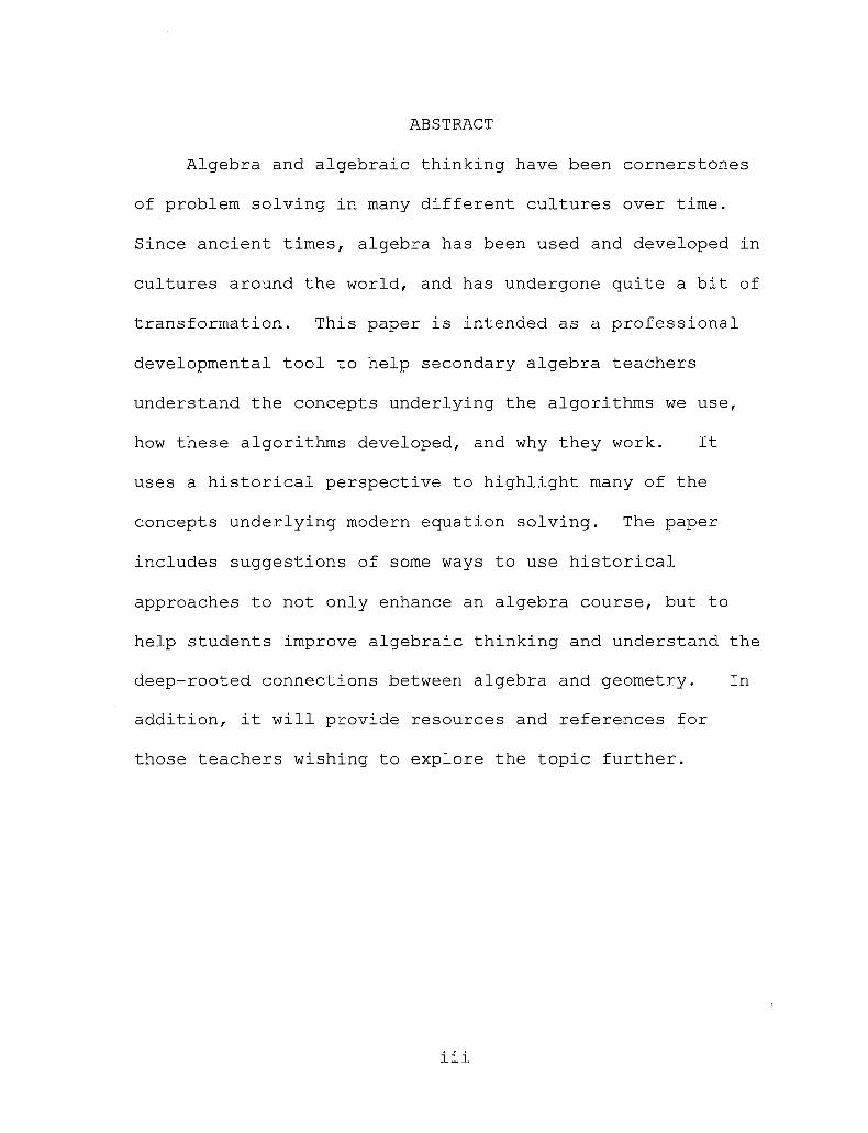
Since the second guess (x2,y2) and the correct solution (x,y)
lie on the same line,
x-x2
Since each of these ratios is equal to the same constant,
then
y-y, y-y2X - Xj x - x2
This equation can be simplified in an effort to solve for x,
the correct solution. 4
y-yr y-y2X - Xj x - x2
Multiplying both sides by (x-x2)(x-Xj) yields
(y-yi)(x-x2) = (y-y2)(x~xx).
Distributing gives
x(T-Ti)-^2(T-yi)=^(j-T2)-xi(T-j'2) •
By regrouping the terms it follows that
xl(y-y2)-x2(y-y1) = x(y-y2)-x(y-yi).
Isolating x provides
Finally, rewrite the equation to find
22

In terms of the original guesses and their errors, the
final result can be represented as follows
Ex • G7 — E2 ■ G,x— —— -—- .
Ei ~ E2
The ancient scholars that developed this method used the
concept of proportionality to derive their solutions, since
in linear equations the change in the output is
proportional to the change in the input (Berlinghoff &
Gouvea, 2004, pl24). This method is similar to the method
of "surplus and deficiency" found in the ancient Chinese
texts. However, this Chinese method employed the use of
one overestimate (surplus) and one underestimate
(deficiency).
Babylonian sources illustrate another variation of
false position in the solution of linear equations. In
some ways the method provides a connection between "false
position" and "double false position." The method involves
making one guess (as in false position), but also
calculating the result if the guess were increased by one
unit (tin essence, making a second fixed guess) . In this
Babylonian variation of false position the solver makes a
23

guess, finds the result, and then calculates the error.
Then, the guess is increased by one unit, and the
difference in the amount of error is observed. Finally,
the proportion by which the change in the error would need
to be multiplied in order to decrease the original error to
zero is calculated. The solution is now obtained by adding
this proportion to the original guess.
Figure 4 depicts a line (y = mx + b). The unknown is the
correct x-coordinate that yields the desired result (To).
Each increase by one on the x axis results in an increase
by the amount of the slope on the y axis. Remember that
slope is calculated by "rise over run." In this variation
of false position, the "run" will always be one. Thus, to
reach the desired result, the question is to find out how
many "slopes" need to be added to go from the original
guess to the correct solution.
24

Figure 4. The Babylonian Variation on False Position
These methods of solving linear equations would not be
familiar to most secondary school students today. However,
with a little time and effort, students would learn to
appreciate where the algorithms that are used today came
from. These methods would reinforce and give a deeper
understanding of proportional reasoning concepts underlying
modern algorithms. These methods and their geometrical
interpretations might also be introduced into the
curriculum for students that are struggling with the modern
25

algorithms, as alternative ways to solve and visualize the
solutions of linear equations.
Applications to the Classroom
Here is an example of a problem that the Ancient
Egyptians solved using the method of false position in
approximately 1650 BC. Each of the problems below will
contain both the historical and modern approaches to the
solution.
Problem 1: From The Rhind Papyrus.2
2Berlinghoff, W.& Gouvea, F. (2004). Math through the Ages. Farmington, ME: Oxton House Publishers.
A quantity; its half and its third are added to it.
It becomes 10.
The Solution: Using current algorithms.
Let x be the unknown quantity.
Writing the' word problem as an equation using the
variable x would yield
1 1 mx + —x + —x = 10.2 3
Combining like terms gives
—x = 10.6
26

Multiplying both sides by the reciprocal of —
isolates x in
Simplifying leads to
Thus the unknown quantity is
The Solution: Using "False Position."
Make a guess (using a number that will work easily
with the denominators 2 and 3):
G = 6
Calculate the result using the guess. Substituting
the guess into the problem yields
«+|(«)+|(6) •
This simplifies to
6 + 3 + 2 = 11 .
Calculate the ratio by which 11 would be multiplied to
get the correct result of 10
11-— = 10 .11
27

Multiplying the original guess by this ratio leads to
Thus, the correct solution is — = 5—.11 11
Here is another example that can be solved using the method
of "false position."
Problem 2: From The Rhind Papyrus (Problem 26) .3
When a quantity is added to one-fourth of itself the
result is 15.
The Solution: Using current algorithms.
Let x be the quantity. Then, writing an equation to
represent the word problem gives1 1C
x + — x = 15 .4
Combining like terms leads to
—x = 15 .4
3 Katz, V. (1998) . A History of Mathematics: An Introduction. Reading, MA: Addison-Wesley Educational Publishers, Inc.
28

Multiplying both sides by the reciprocal of — results
in
x = 15- — .5
Thus, the unknown quantity is 12.
The Solution: Using "false position."
Make a convenient guess (using a number that is a
multiple of the denominator 4):
G = 8 .
Calculate the result using the guess. Substituting
the guess into the problem yields a problem statement:
When the quantity eight is added to one-fourth of
itself (i.e. 2) the result is 10. This statement can
be represented as
8+|(8)-
This simplifies to
8 + 2 = 10 .
Calculate the ratio by which 10 would be multiplied to
get the correct result of 15
10— = 15 .10
29
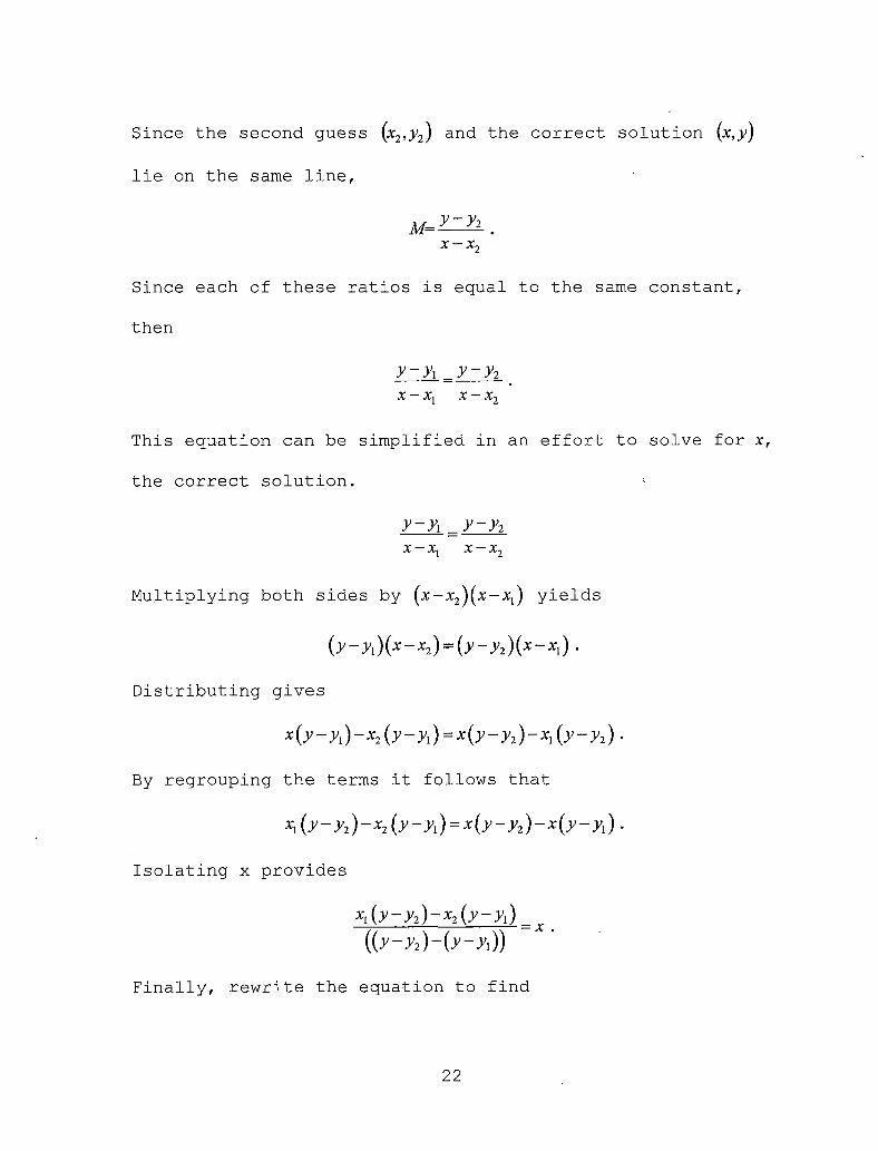
Multiplying the original guess by this ratio leads to
8-—.10
120Thus, the correct solution is -- = 12.10
Here is an example of "double false position" from the
early 1800's.
Problem 3: From Daboil's Schoolmaster's Assistant.4
4Berlinghoff, W. & Gouvea, F. (2004). Math through the Ages. Farmington, ME: Oxton House Publishers.
A purse of 100 dollars is to be divided among four men
A,B,C, and D, so that B may have four more dollars
than A, and C eight more dollars than B, and D twice
as many as C; what is each one's share of the money?
The solution: Using current algorithms.
Let A receive x dollars. Then B receives x+4, C
receives x+4+8, and D receives 2(x+4+8). Then, writing
an equation to represent the word problem gives
x + (x + 4) + (x + 4 + 8) + (2 (x + 4 + 8)) = 100 .
Combining like terms leads to
5x + 40 = 100 .
30

Subtracting 40 from both sides yields
5x - 60 .
Multiplying both sides by the reciprocal of 5 results
in
x = 60 • — .5
Thus A received $12, B received $16, C received $24,
and D received $48.
The Solution: Using "Double False Position."
Make a guess of how much money A receives:
G,=6
Calculate the result using this guess:
6 + (6 + 4) + (6 + 4+8) + (2(6+4 + 8)) = 70 .
This is an underestimate by 30. So, the error (El) is
30.
Make a second guess: G2=8
Calculate the result using this guess:
8 + (8 + 4) + (8 + 4 + 8) + (2(8 + 4 + 8)) = 80 .
This is an underestimate by 20. So, the error (E2) is
20.
31

Since the two errors are the same type (both
underestimates), use the formula for double false
position that is appropriate:
E, • G2— E2 • G,The solution=—-— -- -—L .Ei — E2
Substitution yields
30-8-20-6The solution=-------- .30-20
Simplifying leads to
, n ■ 120The solution=-- .10
So, the solution is 12.
Thus A received $12, B received $16, C received $24,
and D received $48.
An example using the Chinese method of "surplus and
deficiency."
Problem 4: From Jiuzhang (Problem 17) .5
The price of 1 acre of good land is 300 pieces of
gold; the price of 7 acres of bad land is 500. One
5 Katz, V. (1998) . A History of Mathematics: An Introduction. Reading, MA: Addison-Wesley Educational Publishers, Inc.
3.2

has purchased altogether 100 acres; the price was
10,000. How much good land was bought and how much
bad?
The Solution: Using current algorithms.
Let the amount of good land be x acres. Let the amount
of bad land be y acres. The price of x acres of good
land is:
300x acres'— gold pieces per acre = 300xgold pieces.
The price of y acres of bad land is:
500 . 500 i a ■y acres—— gold pieces per acre = -y-y gold pieces.
The total cost would then be
300x + 500- — .7
Thus, the following system of equations can be
developed
x + y = 100
300x +500-— = 10000.7
Solving the first equation for one variable leads to
x = 100-y .
Substituting this equation into the second equation
gives
33

300(100-y) + 500-y = 10000 .
Distributing achieves
30000-300y + ^y = 10000 .
Combining like terms leads to
20000 = ^300-—\ .I 7 /
This can be simplified to
20000 = ^^-y .7
Finally, multiplying both sides by the reciprocal of
1600—-— provides
20000-------1600
Thus, the solution for y is
1600
Substituting this value back into the first equation
(after having solved it for x) yields
x = 100-y = 100-87.5 = 12.5 .
Thus, the amount of good land is 12.5 acres and the
amount of bad land is 87.5 acres.
34

The Solution: Using the Chinese method of "surplus and
deficiency."
Begin by making a guess for the amount of good land:
G} = 5.
Calculate the amount of bad land:
y = 100-5 = 95 .
Now calculate the yield based on the amounts of land:
500-^ = ^.7 7
This is an underestimate by 120007
a "deficiency." Now
make a guess that might give an overestimate, a
"surplus."
G2 =20 .
Calculate the amount of bad land:
y = 100-20 = 80 .
Now calculate the yield based on the amounts of land
300(20)+500-^ = ^0 .
This is an overestimate by 120007
a "surplus."
Thus, to solve the problem, use the formula
EXG2 + E2GX
Ex+E2
35

Substitution yields
Thus, there are 12.5
acres of bad land.
Here is an example of a
Babylonian variation of
Problem 5: From the VAT
<1200
= 12.5 .
acres of good land, and 87.5
problem that was solved using the
"false position."
8389 (Problem 76) . 6
Ej +E2
2One of two fields yields — sila
yields sila per sar (sila and
per sar, the second
sar are measures for
capacity and area, respectively). The yield of the
first field was 500 sila more than that of the second;
the areas of the two fields were together 1800 sar.
How large is each field?
The Solution: Using current algorithms.
Let the first field have an area of x sar. Let the
second field have an area of y sar. Then, x and y need
6Katz, V.(1998). A History of Mathematics: An Introduction. Reading, MA: Addison-Wesley Educational Publishers, Inc.
36

to satisfy the following system of equations
x + y = 1800
-x--y = 500.3 2
Solving the first equation for one variable leads to
x = 1800-y .
Substituting this equation into the second equation
gives
Distributing achieves
1200-—y- —y = 500 . 3 2
Combining like terms and simplifying leads to
700 =—y .6
Finally, multiplying both sides by the reciprocal of
providesex
I o
700-— = y .7
Thus, the y is 600.
Substituting this value back into the first equation
(after having solved it for x) yields
x = 1800-y = 1800-600 = 1200 .
37

Thus, the first field was 1200 sar, and the second
field was 600 sar.
The Solution: Using the Babylonian variation on "false
position."
Make a guess: Let the first field be 900 sar.
Calculate what the second field must have based on the
fixed amount of their sum. Since their sum is 1800
sar, the second field must be 900 sar. Calculating the
difference in their yields results in
150 .
Calculate the error in the result:
500-150 = 350 .
Increasing the guess for the first field by one unit
in turn decreases the guess for the second field by
one unit, and calculating the resulting difference in
the yield gives
Distributing leads to
2 2 1 1 —-900 + —-1-—-900 + —-1 .3 3 2 2
38

Grouping the terms results in
—-900-—-9Ool + f—-1 + —-1^1 ..3 2 ) U 2 )
Factoring the result gives
900 r25
Thus, increasing the guess by one unit has increased
the resulting yield by
2 £_73 2~6 '
Finally, in order to achieve the correct result,
divide the original error by this proportion to find
out how many sar the original guess needs to be
increased:
350h-—= 350-—= 300 .6 7
Thus, the original guess must be increased by 300 sar.
The first field was 1200 sar, and the second was 600
sar.
To create problems that can be solved with the methods
of false position and double false position, fill in the
blanks and change the pertinent information in the
following templates.
39

False Position
An unknown quantity is added to its ____ (half, third,
etc.). It becomes ____ (total amount). What is the
unknown quantity?
Figure 5. Template for False Position
Double False Position
An unknown quantity ____ (type) is added to another
unknown quantity ____ (type), and the result is ____
(constant). ____ (proportion) of the first quantity
together with ____ (proportion) of the second quantity
results in ____ (constant). What are the two
quantities?
Figure 6. Template for Double False Position
40
CHAPTER THREE
QUADRATIC EQUATION-SOLVING
Historical Overview
In 1766 a successor of Islamic prophet Muhammed,
caliph al-Mansur, founded Baghdad, a new capital of his
empire. When the initial impulses of Islamic orthodoxy
gave way to a more tolerant atmosphere, Baghdad soon became
a commercial and intellectual center (Katz, 1998). Over
the next 200 years, the succeeding caliphs set up a world-
renowned library, which included manuscripts from Athens
and Alexandria, and a research institute, the Bayt al-
Hikma. By the end of the ninth century, the most
influential and famous historical mathematical texts had
been translated into Arabic and were being studied in
Baghdad. The Islamic scholars studied the works of Euclid,
Archimedes, Apollonius, Diophantus, Ptolemy, along with
Babylonian and Hindu works.
One of the earliest Islamic algebra texts was written
by Mohammed ibn-Musa Al-Khwarizmi in 825 AD (Katz, 1998).
Within the book itself, and within the title Al-kitab al-
muhtsar fl hisab al-jabr wa-l-muqabala, Al-Khwarizmi used
the term "al-jabr", which would evolve into the word
41

algebra. Al-Khwarizmi noted that what people generally-
wanted was a solution to an equation. His book was a
manual for solving equations. Specifically, Al-Khwarizmi
dealt with three types of quantities: the square of the
unknown, the root of the square (the unknown), and numbers
(constants). Since the Islamic mathematicians did not deal
with negative numbers, coefficients and roots of equations
needed to be positive. The modern term "square root" is
the same idea that Al-Khwarizmi refers to as a "root." The
term "square root" refers to the side length of a square.
The side length is the "root" (the origin) of the square.
root= side length
Figure 7. The "Square Root"
Given a square of area A, the "root" of the square would be
the length of one of its sides. For example, the root of a
42

square of area 9 would be 3. The root of a square of area
2 would be yfl (the "square root" of 2) .
One current method of solving quadratic equations
involves putting all of the terms on one side of the
equation, so that the other side would be zero. This lends
itself to factoring and using the zero product property, or
using the Quadratic Formula (which is just a method of
finding roots so that an equation can be factored).
However, these methods require the use of negative
coefficients in order to attain real solutions. The.
Islamic mathematicians did not accept the use of negative
coefficients/ and thus developed methods to solve quadratic
equations while keeping the coefficients, and solutions,
positive. This led to six types of equations that can be
written using the quantities "squares," "roots," and
"numbers."
1) Squares equal to roots: ax^ =bx
2) Squares equal to numbers: ax^ =c
3) Roots equal to numbers: bx=c
4) Squares and roots equal to numbers: ax^+bx=c
5) Squares and numbers equal to roots: ca^+c = bx
6) Roots and numbers equal to squares: bx + c = ax^
43

Solutions to the first three types of equations could
be achieved via elementary methods. What follows are
illustrations of how types 1-3 might be solved using
familiar methods and notation.
One current method that could be used to solve Al-
Khwarizmi's first type of quadratic equation, ax2 = bx, is
fairly brief. First, divide both sides by of the equation
x. This can be done because of the assumption that x^O. The
solution to Type 1 yields only one solution, as Al-
Khwarizmi did not allow zero as a solution. Dividing
provides
ax2 _ bx
x x
Simplify, and then divide both sides by a,
ax _b
a a
Thus, the solution is
bx = — .
a
The solution method to the second type of Al-
Khwarizmi's equations, ax2=crls similar. First, divide
44

both sides of the equation by ar to yield
ax2 _ c
a a
The next step is to find the length of the side of a square
cwith area —, that is the "root" of the square. In modern or
terms, this refers to taking the square root.
Take the square root of both sides
Thus the solution is
(Remember that Al-Khwarizmi would have only acknowledged
positive solutions.) This type of equation could also be
solved using "false position," as described earlier.
Al-Khwarizmi's third type of equation would not
currently be called a quadratic, as the square term is
missing. Therefore, the solution can be found using
methods that apply to linear equations. The solution to the
equation bx = c can be found by dividing both sides of the
45

equation by b,
bx _c ~b~b'
Thus, the solution is
cx = — .
b
The process of obtaining the solution to Al-
Khwarizmi's fourth type of equation is more complex than
the first three types. Fortunately, it has a geometric
derivation that aids in understanding the algebraic
solution. The equation would take the form ax2+bx = c.
Assume a = 1 for the sake of simplicity. If a were a number
other than one, begin by dividing every term by the value
of a . So we consider the equation x2+bx = c. Represent each
term on the left side of this equation geometrically. The
term x2 can be represented by a square with side length x,
and the term bx can be represented by a rectangle with
sides of lengths x and b . Create a rectangle from these
two figures as shown in Figure 8. Then this new rectangle
must have area equal to c in order to satisfy the equation.
46

x2 +hx = c
ABCD is a square with side length x
ED is a side length representing b
ADEF is a rectangle with area bx
Figure 8. Type 4 Diagram
In an effort to create a square out of this rectangle, so
that we can determine the square's "root," first divide the
rectangle ADEF in half through the midpoints of AF and DE.
Then attach one of these halves to the top of the square,
as shown in Figure 9.
47

Figure 9. Type 4 Gnomon
48

This creates a shape which is sometimes called a gnomon (a
square missing a square). In order to create a complete
bsquare with side length x + —, Tt is necessary to "complete
the square."
This creates Note that boththe equation x + —2
= C +I 2j
equations are different ways to represent the area of the
square KJCG. (Remember that the sum of the areas of
49

rectangles HADG and IJBA together with square ABCD was
equal to
possible
c in the original diagram.) It now becomes
to view the area as the square with side length
the sum
figures
Alternatively,
of the areas of
ABCD, IJBA, and
this
ABCD,
ADGH
new figure can be viewed as
IJBA, ADGH, and KHAI. Since
sum to c, the total area is
the solution becomes clear before
the algebraic solution appears. The solution, x, is the
length of the side of the new large square KJCG minus the
blength of the side of square IAHK, that is —.
Algebraically, after obtaining the
the next step would be to take the square root of both
sides in an attempt to isolate This leads tox.
Considering only positive roots gives
50

Hence
This expression represents the length of the side of the
new square KJCG minus the square IAHK. Negative solutions
were disregarded in this derivation since Al-Khwarizmi
derived his solutions geometrically, so the solution was a
length represented in a diagram.
The solution to Al-Khwarizmi's fifth type of equation
begins in a similar fashion to the solution of the fourth
type. The equation would take the form
x2 + c = bx
where the leading coefficient has again been given the
value of one for the sake of simplicity. Take the case
c>x2, then it becomes possible to represent this equation
with the diagram shown in Figure 11.
51

ax2 +c = bx
ABCD be a square with side length x
HADN be a rectangle with area c
NC is a side length representing b
HBCN is a rectangle with area bx
Figure 11. Type 5 Diagram
To create the desired figure, first construct the
perpendicular bisector of BH and let its intersection with
BH be called G. Then construct a circle with radius AG
centered at G (see Figure 12).
52

Next, construct the intersection K between the circle and
the perpendicular bisector of BH on the side outside of
AHND. Use this segment to construct rectangle RLMH on the
side HG (see Figure 13).
53

54
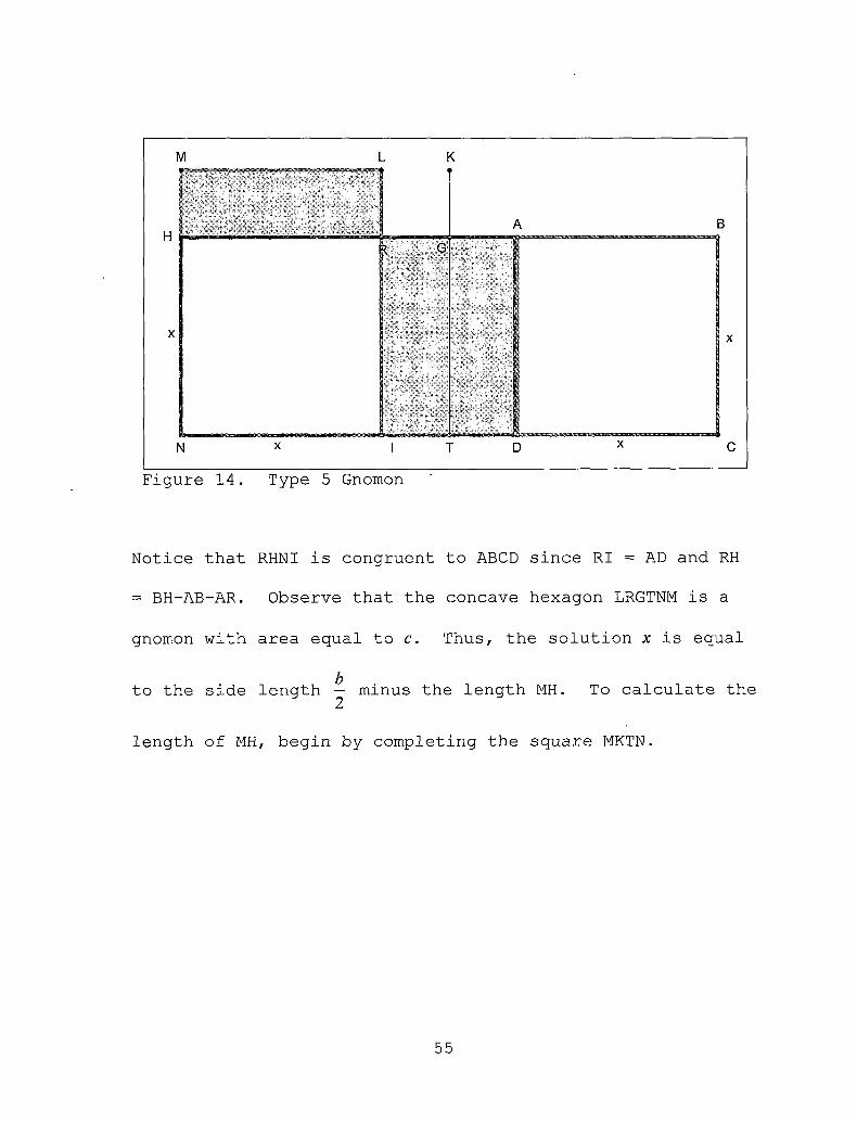
Notice that RHNI is congruent to ABCD since RI = AD and RH
= BH-AB-AR. Observe that the concave hexagon LRGTNM is a
gnomon with area equal to c. Thus, the solution x is equal£
to the side length — minus the length MH. To calculate the
length of MH, begin by completing the square MKTN.
55

Now, MKTN has area c + (/?G!)2 . Now MH is congruent to LR. The
length of LR can be obtained by taking the square root of
the square LKGR. The area of LKGR can be found by
subtracting c (the area of AHNT) from the area of square
bMKTN, a square with side length — . So,
MH = LR =
Thus the solution, x, is
56

The case 0<c<x2 yields a different geometric
interpretation of Al-Khwarizmi's fifth type of equation.
It yields a second positive solution. Figure 16 is
similar to Figure 11, however the area, c, of AHND is
assumed to be smaller than that of square ABCD.
57

In an effort to create a gnomon, from which it will be
possible to derive the value of x, proceed in a manner very
similar to the previous case. The first step is to bisect
segment NC at G and to construct a circle with radius
length NG centered at N.
Figure 17. Type 5 Bisection
Next, construct perpendicular lines from where the circle
intersects HN, and point G. Let I be the intersection of
the circle with HN and construct the square GNIJ.
58

Figure 18. Type 5 Gnomon
Construct a square with length DG off of DG.
Figure 19. Type 5 Completing the Square
59

Now the diagram displays gnomon NDLKJI. Square IJGN is
b missing square LKGD. The solution, x, is equal to — plus
the side length DG (recall that the length NC is equal to
b, and point G bisected NC). To calculate the area of
square LKGD, begin by finding the area of square IJGN.
Then subtract the area of HADN.
Area of LKGD= - c
Thus the side length DG is given by
Finally, the solution, x, is
Al-Khwarizmi found means to solve all the possible
quadratic equations that could be written with positive
coefficients and constants. An illustration of the
solution method for the sixth and final type of Al-
Khwarizmi' s equations can be found in the "Applications to
the Classroom" section. At this point, Al-Khwarizmi still
did not acknowledge the solutions to his equations to be
60
roots of equations. Thomas Harriot developed the idea that
the solutions to quadratic equations were zeros of the
equations. This non-geometric interpretation made it
possible to consider negative solutions. It then became
possible to create a formula that allowed the calculation
of solutions to all quadratic equations, The Quadratic
Formula.
Applications to the Classroom
There is a classic example that Al-Khwarizmi used to
demonstrate his method of "completing the square."
Problem 1: The Classic "Completing the Square" Problem.1
What must be the square which, when increased by ten
of its own roots, amounts to thirty-nine?
The Solution: Using "Completing the Square" pictorially
together with Al-Khwarizmi's verbal description.
You halve the number of roots, which in the present
instance yields five.
This you multiply by itself; the product is twenty-
five .
7 Katz, Victor (1998). A History of Mathematics: AnIntroduction. Reading, MA: Addison-Wesley Educational Publisher, Inc.
61

Add this to thirty-nine; the sum is sixty four.
Now take the root of this which is eight, and
subtract from it half the number of roots, which is
five; the remainder is three.
This is the root of the square which you sought for.
(Katz, 1998, p355)
Students often run straight to the Quadratic Formula
to solve quadratic equations, even when other alternatives
are available. For instance, factoring and using the zero
product property is often a more efficient method to find
the solution(s). The decision to use the Quadratic Formula
or another technique requires students to use critical
thinking and analyzing skills. Like the Quadratic Formula,
Al-Khwarizmi's method of Completing the Square also works
on all quadratics, and when encouraged to use the method,
teachers and students may find that it is often less
complicated than the Quadratic Formula. Practice in
comparing and employing various solution methods can help
students develop such skills.
Problem 2: An Example Comparing the Quadratic Formula to
Completing the Square.
62

Find the root(s) of the equation
y = x2 + 8x + 2 .
The Solution: Using the Quadratic Formula.
For an equation of the form
ax2 + bx + c = 0 ,
the Quadratic Formula is
- b ± 2 - 4acx =-----------------------------.
2a
In order to find the solution(s) to the
y=0, substitute the values a = \, b = 8,and
Quadratic Formula to obtain
-8±V82-4-1--2 x =---------------------------- .
2-1
Simplifying yields
-8±^64 + 8 x =------------------- .
2
Combining terms beneath the square root
-S + y[T2. x =-------------- .
2
Which can be simplified to
-8±6a/2 x —-------------- .
2
equation when
c = -2 into the
gives
63

Factor the 2 out of the numerator to obtain
2(~4±3^)
2
After dividing by the common factor, the roots are
x = -4±3>/2 .
(Teachers may recognize this final step as one which
students frequently make mistakes on.)
The Solution: Using "Completing the Square."
In order to find the roots, substitute zero for y to
obtain
0 = x2 + 8x - 2 .
Completing the square interprets the terms as areas,
so make all of the terms positive yields
x2 + 8x = 2 .
Here is the step-by-step process to find the roots of
the equation.
64

Step 1:
Diagram the areas.
E D C
F
8x
A
X2
(pictures not drawn to
scale)
Step 2:
Divide rectangle FADE in
half through midpoints H
and G. E G D C
F 1 H
Sx
A
X2
Figure 20a. The Steps to Solving an Example of Type 4
65

66

Step 6:
The new square has sides
x + 4 and area 18. Thus,
(x + 4)2 =18 . Taking the
square root of each side
yields x + 4 = ±V18, which can
be simplified to x + 4 = ±3\/2.
Thus, x = -4±3a/2 .
y = x2-10x + 45 .
G 4 D X C
K , *
■(■I®
I
< fv"‘ .
WOSlBWISWiOil
lllii >*4a • « ‘ ; '
OliiOW
The total area is 2+16
Figure 20c. The Steps to Solving an Example of Type 4
Once students become familiar with the diagramming and
geometric concepts underlying the "completing the square"
method, they will be able to apply the method to problems
that do not lend themselves to geometric solutions. This
includes problems that have negative coefficients, and
those that have no real solution (i.e. complex solutions).
Here is one such example.
Problem 3: Find the root(s) of the equation
67

Solution: Using Completing the Square.
Substituting zero for y yields
0 = x2 -10x + 45 .
Rewriting the equation so that the variables are on
one side, and the constant is on the other gives
-45 = x2 -lOx .
In order to create a perfect square from the terms
x2-10x, it is necessary to divide the coefficient of x
by two, and rewrite the problem as
-45 + ? = x2 - 5x - 5x + ? .
The equation, rewritten as a perfect square after
adding 25 to both sides, becomes
-45 + 25 = (x-5)2 .
Simplifying leads to
-20 = (x-5)2 .
Taking the square root of each side, and simplifying
when possible, yields
±2zV5 = x - 5 .
Thus, the roots are
x • 5 ± 2z’a/5 .
68

One application to the classroom would be to ask
students to find the geometric solution to the sixth type
of Al-Khwarizml's equations. Begin by showing students the
solutions to the first five types of equations,
particularly Types 4 and 5. Ask the students to use a
similar diagram to construct the geometric diagram that Al-
Khwarizmi used to derive his solution to the Type 6
equation. This problem is quite challenging, and may
require the use of manipulatives.
Problem 4: Find the geometric representation to display and
derive Al-Khwarizmi's solution to his sixth type of
equation, bx + c = ax2 .
The Solution:
Begin by representing each of the parts of the problem
geometrically. Rectangle ABHR represents area bx.
Rectangle ABHR represents area c. Square ABCD
represents x2 (allow the coefficient of x2 to be one
for the sake of simplicity).
69

ABHR is a rectangle with area c
RD is a side length representing b
RHCD is a rectangle with area bx
ABCD is a square with side length x
x BA
HR
x
CD
Figure 21. The Steps to Deriving Type 6
Begin by bisecting length HC at G and constructing a square
off of HC.
70

Figure 22. Type 6 Bisection
Now, the diagram, shows a square IHGJ with area Orf
Next, construct a square off of side BG with length BG.
71

Now it becomes possible to see that rectangles AMNR
and NIJL are congruent. Therefore the solution, x, is
equal to the sum of length CG and GB. CG was£
constructed to be — . To calculate BG, first find the2
area of square BGLM.
72

The area of BGLM is c+^Y<2,
Thus BG is
<2,
The solution, x, is then
There are questions of varying difficulty levels that
teachers can pose to their students. Students could be
asked to identify the gnomon in one of the figures of the
derivation. In addition, students could be asked to
justify why particular steps of the derivation are allowed.
This includes verifying that pieces of figures are
congruent or similar, and justifying what type of shape a
figure might be (e.g. square).
73

CHAPTER FOUR
CUBIC EQUATION-SOLVING
Historical Overview
Mathematician Fra Luca Pacioli noted that there was
not yet a solution to the general cubic equation in his
book Summa de Arithmetics in the year 1494 (Dunham, 1990).
Specifically, Pacioli was of the opinion that finding a
solution to the general cubic was as likely as squaring ther
circle (Dunham, 1990)8. However, many mathematicians were
working on this problem during the fifteenth and sixteenth
centuries. Sciopine del Ferro took up the challenge to
find the solution to the general cubic while teaching at
the University of Bologna between 1500 and 1515 (Katz,
1998). In fact, del Ferro did find a method for solving
the cubic, but not to the general form. The general form
of a cubic would now be written as
8 Recall that squaring a circle was once considered an extremely difficult task, and was later proven to be impossible. (For more information, see: Dunham, W. (1990). Journey through Genius. New York, NY: Penguin Books.)
ox3 + Z>x2 + ex + d = 0 .
74

The solution method del Ferro found solved depressed
cubics, those without a square term:
ax3 + ex+ d = 0 .
Curiously, his method of finding a solution was not
publicized, but rather, was kept a secret. This secrecy
was a function of the academic attitude at the time. The
current trend in academia is for professors to publish new
results as quickly and often as possible. However, in the
sixteenth century, university professors were expected to
challenge others, and to meet the challenges of others.
Their professorial worth was on the line every time they
took up a challenge, as was the security of their jobs.
For this reason, del Ferro did not publish his results.
Rather, he kept his breakthrough a secret shared with no
one but his student Antonio Maria Fior, and his successor
Annibale della Nave, whilst on his deathbed. Fior and Nave
did not publicize the solution, but word spread that the
solution to the cubic was known. Soon another
mathematician named Niccolo Fontana (best known as
"Tartaglia") boasted that he too knew the solution to the
cubic.
75

Fior publicly challenged Fontana in 1535. Each
mathematician provided problems for the other to solve.
For example, "A man sells a sapphire for 500 ducats, making
a profit of the cube root of his capital. How much is that
profit?" This problem could be written algebraically as
x3 + x = 500 .
Tartaglia discovered the solution to this cubic problem,
while Fior was unable to solve many of Tartaglia's non-
cubic mathematical questions (Katz, 1998). For this
reason, Tartaglia was declared the winner of the
mathematical duel. His prize was 30 banquets prepared by
Fior, which Tartaglia declined in favor of simply having
the honor of being the victor (Katz, 1998).
Gerolamo Cardano, a mathematician giving public
lectures on mathematics in Milan, heard about Tartaglia's
solution to the cubic. After many entreaties, Tartaglia
agreed to share his method with Cardano, provided that
Cardano would not publish these methods. This is how
Tartaglia solved the cubic x3+cx = d.
jWhen the cube and its things near
2Add to a new number, discrete,
3Determine two new numbers different
76

4 By that one; this feat
5Will be kept as a rule
6Their product always equal, the same,
7To the cube of a third
sOf the number of things named.
9Then, generally speaking,
10The remaining amount
H0f the cube roots subtracted
12Will be your desired count.
(Katz, 1998, p359)
Line 1 refers to x3 (the cube) and ex (its things). In Line
2, Tartaglia is referring to creating the term x3+cx = d.
Let v and w be the two new numbers in Line 3. Let their
difference be represented by v-w-d in this line. Lines 6
Thus, Lines 9 through
12 say that Vv-Vw is the solution to the problem. This
can be checked by substituting this solution into the
original cubic x3+cx = d. This would initially give the
77
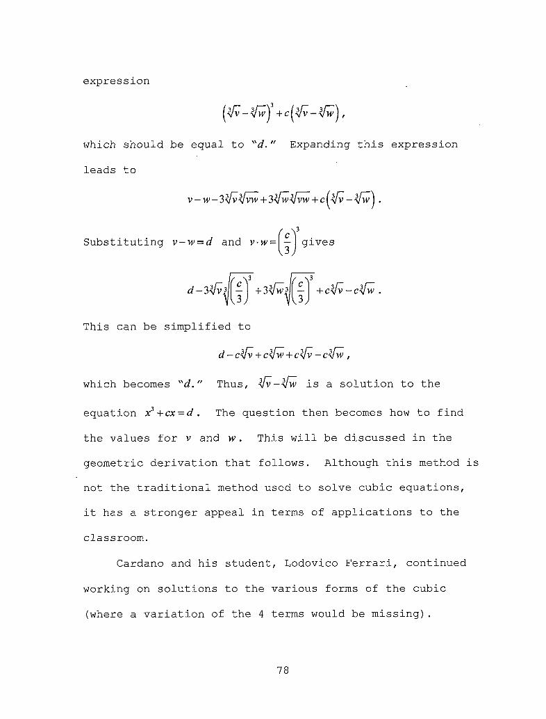
expression
which should be equal to "d." Expanding this expression
leads to
Substituting v-w = d and gives
+ c^/v —ctfw
This can be simplified to
d - ctfv + c-Vw + cl/v — c\lw ,
which becomes "d." Thus, y/v-yfw is a solution to the
equation x3+cx = d. The question then becomes how to find
the values for v and w. This will be discussed in the
geometric derivation that follows. Although this method is
not the traditional method used to solve cubic equations,
it has a stronger appeal in terms of applications to the
classroom.
Cardano and his student, Lodovico Ferrari, continued
working on solutions to the various forms of the cubic
(where a variation of the 4 terms would be missing).
78

Cardano investigated del Ferro's papers and found that he
had discovered the solution to the cubic before Tartaglia.
Anxious to publish the solutions to the cubic, and not
wanting to betray Tartaglia, Cardano used the fact that del
Ferro had discovered the solution first to evade his
promise of secrecy. Cardano published Ars Magna, sive de
Regulis Algebraicis (The Great Art, On the Rules of
Algebra) (Katz, 1998). Cardano's Formula (in modern
notation) to solve the cubic x3+cx = d is
Before examining Cardano's method, it is interesting
to note that both Niccolo Fontana and Gerolamo Cardano both
led fascinating lives. Fontana was disfigured as a boy
when a soldier slashed his face with a sword. The legend
tells that he survived only because a dog licked his wound,
causing it to heal (Dunham, 1990). Due to the serious
injury to his face, Fontana had a speech impediment. His
nickname became Tartaglia (The Stammerer), and he is best
known by that nickname today (Dunham, 1990). Gerolamo
Cardano was plagued by infirmities throughout his life
(Dunham, 1990). He kept track of his many afflictions, and
79

left a detailed accounting of them in his autobiography.
Cardano had a vision of a woman in white in a dream. When
he later met a woman that he felt resembled that of his
dream, he married her. When his wife died, leaving him
with two sons and a daughter, Cardano was left to raise his
children alone. He writes that disaster struck in the form
of a "wild woman," whom his eldest son Giambattista married
(Dunham, 1990). The couple soon produced a male child
named Fazio. Unfortunately, the wife boasted that none of
the children were Giambattista's. Giambattista prepared a
cake laced with arsenic that killed his wife. He was
subsequently convicted and beheaded. Cardano raised Fazio
as a son, and the relationship thrived. Near the end of
his life, Cardano was jailed for heresy against the Church
of Italy for several issues, including writing a book
titled In Praise of Nero. These two mathematicians of the
16th century led fascinating lives, and their stories serve
as a reminder that mathematicians are humans too.
Tartaglia and Cardano both played important roles in
deriving the solution to cubic equations. Cubics of the
form x3+cx = d are considered "depressed" because the square
term is missing. Cubics that begin in the form x3+bx2 + cx = d
80

can all be rewritten as depressed cubics. In fact,
substituting
bx = m —
3
(where b is the coefficient of the second degree term)
results in a cubic in m with no square term. Substituting
this value for x yields
Simplifying leads to
3 , 2 b2 b3 ,2 2b2 b3 cbm —bm H---m--------- \-bm-------- m-\------- \-cm------ =
3 27 39 3
Finally, by grouping the terms, the equation becomes
m3 +(~b + b)m2 +2b2
3
The coefficients of the square term become zero, thus
creating a cubic with no square term. This is a depressed
cubic, for which it is possible to use Cardano's Formula.
Hence, it is possible to find a solution to all cubic
equations using Cardano's Formula. Keep in mind that all
cubic graphs have at least one real root, as they are odd
functions. Quantitatively this means that the range of the
graph will be all real numbers, guaranteeing hence that the
81

graph will have at least one real root. The Intermediate
Value Theorem (commonly covered in calculus) guarantees
that there exists at least one real root. The Intermediate
Value Theorem states that if f(x) is continuous on the
interval [a,b], and k lies between f(a) and f(b), then /(x)
will have value k for some value of x on the interval [a,b].
Essentially, the function cannot get from one point to the
other without crossing horizontal line y = k .
82

A geometric understanding for Cardano's solution to
the cubic equation requires some three-dimensional
diagrams. The following two-dimensional nets can be used
to create the shapes necessary to see Cardano's solution.
83

The Nets for the Cubic Derivation
u
NetC
u
,'NetCi ;
u
NetD i
u
NetD
84

Each of these nets, when cut and folded along the lines
provided, creates a three dimensional shape that will be
used to construct the geometric derivation of Cardano's
solution to the equation
x3 + ex = d .
Note that this geometric derivation ties together with
Tartaglia's poem to find the solution of a cubic (discussed
earlier). In fact, w3 (the small cube) corresponds to
Tartalia's w3 . In addition, x3corresponds to Tartaglia's
v3. Geometrically, this would refer to a cube and a
rectangle added together to create "d." Let Figure 1 (blue
cube) represent x3 . Then Figure 2 (red cube) is the cube
that is missing after the pieces are put together represent
m3 (the piece will not be put together with the rest). Two
of Figure 3, the pink rectangular prisms representing
ux(u + x), are necessary to complete the picture. Figure 4,
the yellow prism represents x2u . Figure 5, the green
rectangular prism represents xu2 . When all the figures are
cut out and attached to each other (excluding Net B), they
comprise a large cube with dimensions (x + w)3— u3 . Thus, the
three dimensional shape implies that the large cube (which
85

is missing a small cube) is equal to the sum of its parts.
This shape is analogous to the quadratic "gnomon," and
might therefore be named a "cubic gnomon."
(x + w)3 — w3 = x3 + 3x2w + 3xw2.
Factoring produces
(x + m)3 - u3 = x3 + xu[3(x + «)].
Regrouping the terms leads to
(x + u)3 — u3 = x3 + x[3m(x + w)].
This sum represents a cube and six rectangular prisms added
together. In other words, this sum is the "d" in the
original equation x3+cx = d. Thus, 3u(x + u), the rectangles,
is the value "c" in the equation. Consequently, it is
possible to write "d" as the original form from which
x3 + x[3w(x + w)] was derived,
(x + w)3 - u3 .
Hence,
d = (x + u)3-u3 and c = 3w(x + w)
This implies that
cx + u = — .
3u
86

With substitution, it is possible to derive that
Cubing each term leads to
d = -C ^--u327u3
Multiplying both sides by w3 generates
c3 d -u3 =-------u6
27
Writing an equation in terms of u leads to
— = u + du .27
In an effort to write a quadratic in u3 , substitute y = u3
into the previous equation. This leads to
2 W C" y +dy = —
27
The Quadratic Formula provides the solution
Notice that the negative solution is not included, as
negative solutions were disregarded at the time. From
which is follows that
d fj2--- kJ--- 1--- .
2 V 4 27
87

Taking the cube root of both sides leads to
Recall that originally d = (x + uf-u3. Solving the equation
for x gives x = \d + u3-u. Substituting the derived values
for "u" and "m3" provides
This leads to Cardano's solution for x
Applications to the Classroom
The cube root is analogous to the square root, which
is described in Figure 1. The square root refers to the
length of a side of a square with a desired area, while the
cube root refers to the length of a side of a cube with a
desired volume.
Although Cardano expanded on his Islamic predecessors
by including the possibility of negative solutions, he was
still not able to find all the possible solutions to cubic
equations. Rafael Bombelli continued to expand on, and
88

refine, the work of Cardano. Bombelli wrote a book that
contained a logical progression from linear to quadratic to
cubic equations. He also included the idea that it seemed
possible to take the square root of a negative number,
something that is encountered when using Cardano's formula
for some cubic equations. He used notation that was a
stepping stone toward the notation currently used in
algebra. For example, Bombelli began writing R.Sq. to
represent the square root. Bombelli also noted that it was
possible to take the cube root of numbers that were
negatives. He noted that this required a,different set of
rules for these new numbers, which he called "plus of plus"
and "minus of minus" (Katz, 1998). In modern terms,
Bombelli had begun working with imaginary numbers.
Bombelli's promotion of the existence of imaginary numbers
allowed the use of Cardano's Formula even when the sum
beneath the root would be negative.
Problem 1: Use Cardano's Formula to solve a cubic equation.
89
Use Cardano's Formula to get one real solution of the
equation x3+63x=316. Then, use this solution to find
the remaining solutions to the equation.

The Solution:
Cardano's Formula gives
as the solution to equations of the form
x3 + ex = d .
Thus, substituting the values of c and d into Cardano's
formula gives
^[316 |3162 633 J 316 I3162 633H 2 J 4 +27 \ 2 + V 4 + 27 '
Simplifying this equation results in
x = V343 -V27 = 7-3 = 4 .
And so it follows that x-4 is a factor of the original'
cubic. It is now possible to use long division or
synthetic division to determine the quadratic by which
x-4 would be multiplied in order to obtain the1
original cubic. The division of x3+63x-316 by x-4
results in x2+4x + 79. And so it follows (by the
Quadratic Formula) that the remaining solutions of the
original cubic are -2 + 5/V3 .
90

In some problems, students will find themselves faced
with the issue of taking the cube root of a value they are
unfamiliar with. Here is an example that would be the
first step in solving this type of problem.
Problem 2: An Example Involving the Cube Root of an
Imaginary Number.
a) Verify that (5+ /)3 =110 + 74/.
b) Conclude that V110-74/ =5 + z .
c) Similarly show that Vl 10-74/ = 5-z
d) Use Cardano's Formula to find one real solution to
x3 — 78x = 220 .
The Solution:
a) Using the binomial theorem, expand
(5+>y =(sy+3(5y(/)+3(5Xo2+(/y.Simplifying this expression gives the desired result
(5+ /)3 =110 + 74/
b) To show that
V110-74/ =5-/,
first cube both sides
110-74/ = (5-z)3 .
91

Then use the binomial theorem to expand the
expression
(5-i)’=(5)!+3(5)!(-0+3(5X-02+(-?•
Simplifying this expression gives the desired result
(5-z)3 =110-74/.
c) Substitute c=-78 and J=220 into Cardano's
Formula to obtain the real solution
2202 (-78)3 J 220 | 12202 ! (~78)~4 + 27 V 2 +V 4 + 27
Simplifying the terms under the cube root leaves
x = Vl 10+ 7-5476 -V-l 10 + 7^5476 .
Rewriting in complex form results in
x = Ml 10+ 74/ - V-110+ 74/ .
Factoring a negative one out of the second cube root
gives
x = Ml 10+ 74/ + Ml 10-74/ .
Note that M-l 10 + 74/ = 3/(-l)(110-74/) = -Ml 10-74/ .
Substituting the known quantities from parts a) and
92

b) leaves
x = (5 + z)+(5-z).
Hence, one of the solutions to the cubic is
x = 10 .
Problem 3: Large templates for building the geometric
representation for the equation x3+6x = 20 are provided.
Create the three dimensional figure that represents the
equation. Note that the figures are drawn to the scale
necessary to create the geometric representation of this
equation. Students could actually measure the side length
of the appropriate pieces to find the desired solution.
93

Figure 26. Cubic Net A
94

Figure 27. Cubic Net B
95

nets.)
Cubic Net C
96

(Remember that the figure requires
three of these nets.)
Figure 29. Cubic Net D
97

98

99

Figure 32. Assembled Cubic Pieces (Back View)
100

Figure 33. "Completed" Cubic
101

CHAPTER FIVE
CONCLUSIONS
Many would agree that the teaching of mathematics at
all levels can be enriched by historical reflection. This
enrichment may be most acute at the secondary school level.
At this point, students begin to grasp the wide scope of
mathematics. Discovering the power of mathematics may
cause students to become overwhelmed. Knowledge of the
historical context behind the concepts may alleviate the
sense of confusion on the part of the student. It may also
present feasible responses to the famous "When will I ever
use this?" This question is one which secondary
mathematics teachers face on a daily basis. Presenting the
history behind topics allows students to see how the
algorithms and ideas they are currently learning evolved
over the course of hundreds of years.
Atival (1995) found that most mathematics taught in
the secondary schools today is devoid of historical
context. Essentially, the students view the topic as
coming only from the classroom teacher. The teacher shows
the students how to do the problem, and then decides
whether they have done it correctly or not. This situation
102
is harmful to the teaching of mathematics, a cumulative
topic, as it presents the information as isolated and
unrelated to the many other concepts that aided in its
development (Atival, 1995). When students learn that the
topics presented are products of a human endeavor that
spans hundreds of thousands of years ago through the hard
work or many people, it creates a sense of interest in the
material, making it more personal and relevant.
The use of manipulatives and models has been shown to
be extremely valuable in increasing students' understanding
of a subject (National Council of Teachers of Mathematics,
1989). If the manipulatives and models are well-chosen,
then the operations on them help to draw general
conclusions about what happens in the more abstract cases.
In addition, the use of manipulatives motivates those
students who are more kinesthetic than auditory or visual.
The act of moving pieces around will help the student
understand and remember the material.
The examples and explanations in this paper offer both
visual and kinesthetic learners an opportunity to excel.
In addition, the derivations of the steps to equation
solving connects geometry with algebra. In doing so, it
strengthens the skills and understanding in both areas.
103

The material within this paper addresses several of
the content standards that California teachers are expected
to address. Specifically, the material on linear equation
solving addresses all or part of the following Algebra 1
standards9:
9 Standards taken from the California Department of Education website: www.cde.ca.gov.
2.0 Students understand and use such operations as taking
the opposite, finding the reciprocal, taking a root,
and raising to a fractional power. They understand and
use the rules of exponents.
5.0 Students solve multistep problems, including word
problems, involving linear equations and linear
inequalities in one variable and provide justification
for each step.
9.0 Students solve a system of two linear equations in two
variables algebraically and are able to interpret the
answer graphically. Students are able to solve a
system of two linear inequalities in two variables and
to sketch the solution sets.
11.0 Students apply basic factoring techniques to second-
and simple third-degree polynomials. These techniques
include finding a common factor for all terms in a
104

polynomial, recognizing the difference of two squares,
and recognizing perfect squares of binomials.
19.0 Students know the quadratic formula and are familiar
with its proof by completing the square.
20.0 Students use the quadratic formula to find the roots
of a second-degree polynomial and to solve quadratic
equations.
21.0 Students graph quadratic functions and know that their
roots are the x- intercepts.
22.0 Students use the quadratic formula or factoring
techniques or both to determine whether the graph of a
quadratic function will intersect the x-axis in zero,
one, or two points.
In addition, the quadratic equation-solving addresses
the following Geometry standards entirely or in part:
2.0 Students write geometric proofs, including proofs by
contradiction.
4.0 Students prove basic theorems involving congruence and
similarity.
5.0 Students prove that triangles are congruent or
similar, and they are able to use the concept of
corresponding parts of congruent triangles.
105

8.0 Students know, derive, and solve problems involving
the perimeter, circumference, area, volume, lateral
area, and surface area of common geometric figures.
9.0 Students compute the volumes and surface areas of
prisms, pyramids, cylinders, cones, and spheres; and
students commit to memory the formulas for prisms,
pyramids, and cylinders.
11.0 Students determine how changes in dimensions, affect
the perimeter, area, and volume of common geometric
figures and solids.
16.0 Students perform basic constructions with a
straightedge and compass, such as angle bisectors,
perpendicular bisectors, and the line parallel to a
given line through a point off the line.
17.0 Students prove theorems by using coordinate geometry,
including the midpoint of a line segment, the distance
formula, and various forms of equations of lines and
circles.
Although the cubic equation and its solutions are not
addressed in the secondary mathematics curriculum, it is a
valuable way to tie together several of the standards from
the Advanced Algebra curriculum:
106

3.0 Students are adept at operations on polynomials,
including long division.
4.0 Students factor polynomials representing the
difference of squares, perfect square trinomials, and
the sum and difference of two cubes.
5.0 Students demonstrate knowledge of how real and complex
numbers are related both arithmetically and
graphically. In particular, they can plot complex
numbers as points in the plane.
6.0 Students add, subtract, multiply, and divide complex
numbers.
7.0 Students add, subtract, multiply, divide, reduce, and
evaluate rational expressions with monomial and
polynomial denominators and simplify complicated
rational expressions, including those with negative
exponents in the denominator.
20.0 Students know the binomial theorem and use it to
expand binomial expressions that are raised to
positive integer powers.
Additional References
If the reader wishes to pursue the topic further, here
are some additional references that may be helpful.
107

Bashmakova, I. & Smirnova, G. (2000). The Beginnings
and Evolution of Algebra. Washington DC: Mathematical
Association of America.
Cardano, G. (1993). Ars Magna, or the Rules of
Algebra. New York: Dover Publications.
Cardano, G. (forthcoming). Autobiography. Cambridge,
MA: Harvard University Press.
Fauvel, J. & Gray, J. (Eds.) (1988). The History of
Mathematics: a Reader. Basingstoke: Macmillan Press Ltd.
Grattan-Guinness, I. (2000). The Rainbow of
Mathematics: A History of the Mathematical Sciences. New
York: W.W. Norton.
Rosen, F. (Ed.) (1997). The Algebra of Mohammed ben
Musa. Frankfort am Main: Institute for History of Science
at the Johann Wolfgang Goethe University.
108

REFERENCES
Atival, S. (1995). The History of Mathematics Can
Help Improve Instruction and Learning. In F. Swetz, J.
Fauvel, 0. Bekken, B. Johansson, V. Katz (Eds.), Learn from
the Masters (pp 3-12). Washington, DC: Mathematical
Association of America.
Berlinghoff, W.& Gouvea, F. (2004). Math through the
Ages. Farmington, ME: Oxton House Publishers.
Boyer, C. (1968). A History of Mathematics. New York,
NY: John Wiley & Sons.
Bunt, L., Jones, P., & Bedient, J. (1976). The
Historical Roots of Elementary Mathematics. Englewood
Cliffs, NJ: Prentice-Hall Inc.
Dunham, W. (1990) . Journey through Genius. New York,
NY: Penguin Books.
Eves, H. (1956) . An Introduction to the- History of
Math. New York, NY: Rinehart & Co.
Katz, Victor (1998). A History of Mathematics: An
Introduction. Reading, MA: Addison-Wesley Educational
Publisher, Inc.
National Council of Teachers of Mathematics (1989).
Historical Topics for the Mathematics Classroom.
109

Newman, J. (1956). The World of Mathematics. New
York, NY: Simon & Schuster.
Swetz, F. (1994). From Five Fingers to Infinity.
Chicago, IL: Open Court.
110