Robert Schuman

Miami-Florida European Union Center of Excellence

The euro before the financial crisis of 2008: An integrating and stabilizing factor

María Lorca-Susino

Vol. 13 No.9 June 2013

Published with the support of the European Commission

8

1

The Jean Monnet/Robert Schuman Paper Series The Jean Monnet/Robert Schuman Paper Series is produced by the Jean Monnet Chair of the University of Miami, in cooperation with the Miami-Florida European Union Center of Excellence, a partnership with Florida International University (FIU).

These monographic papers analyze ongoing developments within the European Union as well as recent trends which influence the EU’s relationship with the rest of the world. Broad themes include, but are not limited to:

The collapse of the Constitution and its rescue by the Lisbon Treaty The Euro zone crisis Immigration and cultural challenges Security threats and responses The EU’s neighbor policy The EU and Latin America The EU as a model and reference in the world Relations with the United States

These topics form part of the pressing agenda of the EU and represent the multifaceted and complex nature of the European integration process. These papers also seek to highlight the internal and external dynamics which influence the workings of the EU and its relationship with the rest the world.

Miami - Florida European Union Center: Jean Monnet Chair Staff:

University of Miami Joaquín Roy (Director) 1000 Memorial Drive Astrid Boening (Research Associate) 101 Ferré Building María Lorca (Research Associate) Coral Gables, FL 33124-2231 Maxime Larivé (Research Associate) Phone: 305-284-3266 Beverly Barrett (Associate Editor) Fax: (305) 284 4406 Dina Moulioukova (Research Assistant) Web: www.miami.edu/eucenter

Florida International University Rebecca Friedman (FIU, Co-Director)

International Editorial Advisors: Iordan Gheorge Bărbulescu, National University, Bucarest, Romania Federiga Bindi, University Tor Vergata, Rome, Italy Francesc Granell, University of Barcelona, Spain Carlos Hakansson, Universidad de Piura, Perú Fernando Laiseca, ECSA Latinoamérica Finn Laursen, Dalhousie University, Halifax, Canada Michel Levi-Coral, Universidad Andina Simón Bolívar, Quito, Ecuador Félix Peña, Universidad Nacional de Tres de Febrero, Buenos Aires, Argentina Lorena Ruano, CIDE, Mexico Eric Tremolada, Universidad del Externado de Colombia, Bogotá, Colombia Blanca Vilà, Autonomous University of Barcelona

2

The euro before the financial crisis of 2008: An integrating and stabilizing factor

By María Lorca-Susino1

Introduction

The main focus of this study is to examine whether the euro has been an economic, monetary, fiscal, and social stabilizer for the Eurozone. In order to do this, the underpinnings of the euro are analysed, and the requirements and benchmarks that have to be achieved, maintained, and respected are tested against the data found in three major statistics data sources: the European Central Bank’s Statistics Data Warehouse (http://sdw.ecb.europa.eu/), Economagic (www.economagic.com), and E-signal.

The purpose of this work is to analyse if the euro was a stabilizing factor from its inception to the

break of the financial crisis in summer 2008 in the European Union. To answer this question, this study analyses a number of indexes to understand the impact of the euro in three markets: (1) the foreign exchange market, (2) the stock market, and the Crude Oil and commodities markets, (3) the money market.

The foreign exchange market is studied to present the evolution of the euro as a common currency

and its relationship with certain foreign exchange indexes and currencies. The innovative touch of this work is that it presents the evolution of the German mark that although it is no longer in circulation, its trading value was continued for some years by Future Source (www.futuresource.com). This section of the study sheds lights on two important debates about the existence of the common currency. One dealt with the possibility of the euro ending with the dollar hegemony, and the second debate deals with the possibility of the British pound joining the euro.

Secondly, this work studies the evolution of the euro and its relationship with two important stock

market indexes—the Dow Jones Industrial Average (DJIA) and the Deutscher Aktien IndeX 30 (DAX)— to show that the high value of the euro has granted European investors access to invest in the stock market on both side of the Atlantic. Also, this section emphasizes the importance and significance of the relationship between the euro and the price of oil and certain commodities due to their direct effect on price stability, inflation, purchasing power, and living standard. The analysis concludes that the high value of the euro has helped with the cost of commodities and oil much-needed for economic growth. Although, these are commodities priced in U.S. dollars, the value of the euro has made these commodities more affordable.

1 María Lorca-Susino, Ph.D. is full-time lecturer of economics at the University of Miami as well as Associate Editor at the European Union Center at the University of Miami. She holds a Master in Business Administration in Finance, a Master of Science in Economics and a Bachelor of Arts and Science in Political Science (University of Miami). She has recently published “The Euro in the 21st Century” (Ashgate). Her research interests include comparative political economy, with a special interest in the European Union and Spain. Her most recent publications are all available online at www.miami.edu/eucenter.

3

Finally, this work takes a look at the effect of a strong euro on inflation. Depending on the evolution of the price index and inflation, the European Central Bank (ECB) decides on the “price of money” and adjusts the money markets accordingly. For this reason, the third market analysed is the evolution of the money market and its relationship with the euro. This section concludes that the US and the Eurozone have their own business cycles and that the ECB has maintained its independence and its commitment to price stability.

Literature review

The euro´s depiction as “the most dramatic change in the international monetary system since President Nixon took the dollar off gold in 1971,¨ places the creation of the EMU and the introduction of the euro among the major economic, political, and historical events of the 20th century.

The much-debated issue of whether a group of countries should relinquish their national currency

and adopt a common one was first introduced by R. Mundell, who pioneered the ¨theory of optimum currency area” in Madrid (Spain) where he presented the idea on a paper titled “A plan for a European Currency” during the conference on “Optimum Currency Areas.” This theory studies how countries with a monetary union and common currency adjust when affected by asymmetric economic shocks. According to Mundell, countries with a monetary union and a common currency would not be able to properly absorb asymmetric shocks unless, among other circumstances, wages are flexible and labor mobility is a reality. Counter to this view, the European Commission, in its document entitled ¨One Market, One Money,¨ sets forth a defence arguing that such countries suffer fewer asymmetric economic shocks.

The adoption of the euro has therefore stirred a debate between defenders of the euro and

Eurosceptic. Pedro Schwartz explains that the defenders of the euro acknowledged that a single European currency and a single European central bank were better suited to achieve monetary stability, while the task of pursuing active macroeconomic and welfare policies should be delegated to the national governments. Still, experts criticizing the euro, Schwartz explains, ¨also want an active monetary and social policy, but they think it should be put into effect within a sovereign national state.¨ Other well- recognized defenders of the euro include R. Mundell and F. Bergsten. They believed the creation of the EU and the introduction of the euro to be positive, not only because they were convinced that the EU would experience political and economic stability, but also because they expected that the euro would eventually “challenge the dollar for global supremacy.” Europhiles believe that the only way the euro can consolidate its role as an international currency is if the Eurozone improves its economic performance. This view is reflected in Masahiro Kawai’s suggestion that “Euroland has already achieved convincing price stability but achievement of dynamic growth may also be necessary for the euro to effectively challenge the dollar.” Fred Bergsten has explained that adopting the euro not only forces countries to give up their national currencies, but also pressures them to relinquish the two major national policy instruments: monetary policy and exchange rate policy. Furthermore, the fiscal policy of member states was trimmed as well because the adoption of the Stability and Growth Pact (SGP) was designed to eliminate part of discretionary national fiscal policy of the government. The introduction of the Convergence criteria and the EMU provided countries with a “discipline” mechanism that has incorporated the usage of fiscal policies to comply with the Stability and Growth Pact. Bergsten pointed out that a currency union would only be effective as long as the countries involved possess the requisite internal adjustment devices.

4

Eurosceptics have been since 1992 persistently forecasting the demise of the euro and that of the EMU. They claim that that some countries in Europe might not be well-suited to adopt a common currency because there are major discrepancies between countries such as differing inflations rates, exchange rates behaviours and low degrees of labor mobility. This term derives from “eurosclerosis,” an expression used in the 1980’s to describe the economic situation of high unemployment and low growth, suffered by most of the EU members. Diane Coyle (2005, 1) states that “the term eurosclerosis was coined to describe the furring of Europe’s economic arteries.¨ Since the 1980’s, eurosceptics have been arguing against the feasibility of the EMU and the euro as a integrating and solid common currency. They emphasize what they believe is a lack of accountability in the implementation of the SGP and the slow pace of structural reforms. They view this lack of economic coherence as a consequence of insufficient and incomplete integration, which is essential to the functioning of the EU as a unitary actor.

Eurosceptics have systematically forecasted not only that the euro will never challenge the U.S.

dollar’s dominance as an international or global currency, but also that the Eurozone will never succeed as a common currency area. For Charles Wyplosz’s (1999, 76) the EMU and the euro are part of ¨the hidden agenda of Europe’s long-planned adoption of a single currency¨ as well as his pessimistic belief that the euro will only dominate in what he calls the ¨euro-time zone¨ (89). Others predicted that the EMU and the euro would not have a significant effect on the overall economic performance of the euro area (Levy 2004, 71). They also speculated that the Eurozone’s persistent growth shortfall would not help improve the elevated unemployment rate of the 1990’s and that the euro will not last as a common currency.

Recent studies have found that since the EMU was established, there has been an increased

convergence and similarity of national business cycles within Europe. In fact, according to Stefano Fantacone and P. Parascandolo one of the preconditions for monetary union is the convergence of the participating countries´ growth cycle. Nevertheless, proponents and critics of the common currency agree that the slow growth in the Eurozone is mainly due to lack of structural reforms. Martin Baily and Jacob Kirkegaard also agree that most changes undertaken by Eurozone members are structural changes mainly related to labor and capital markets.

Technical matters and computer program technicalities

This study presents a total of 27 figures to study three markets. Two of these figures (Figures 26 and 27) have been collected directly from Economagic. These figures have been graphed showing recessions provided by the National Bureau of Economic Research (NBER) which is the only organization that can officially announce U.S. business cycle expansions and contractions. For the rest of the figures the numerical data has been collected from Future Source and the European Central Bank (ECB) in Excel format and converted into Metastock readable data using a professional data converter program, the Downloader. This data was graphed with the consent of the Omega Research Pro-Suit 2000i program.

Figures 1 through 25 present a wide variety of custom-made indexes strengthened by the statistic

reliability of a number of significant statistical methods such as the covariance, de-trend, and simple and exponential moving averages. Table 1 provides a summary of which figures have been analysed using which statistic method.

5

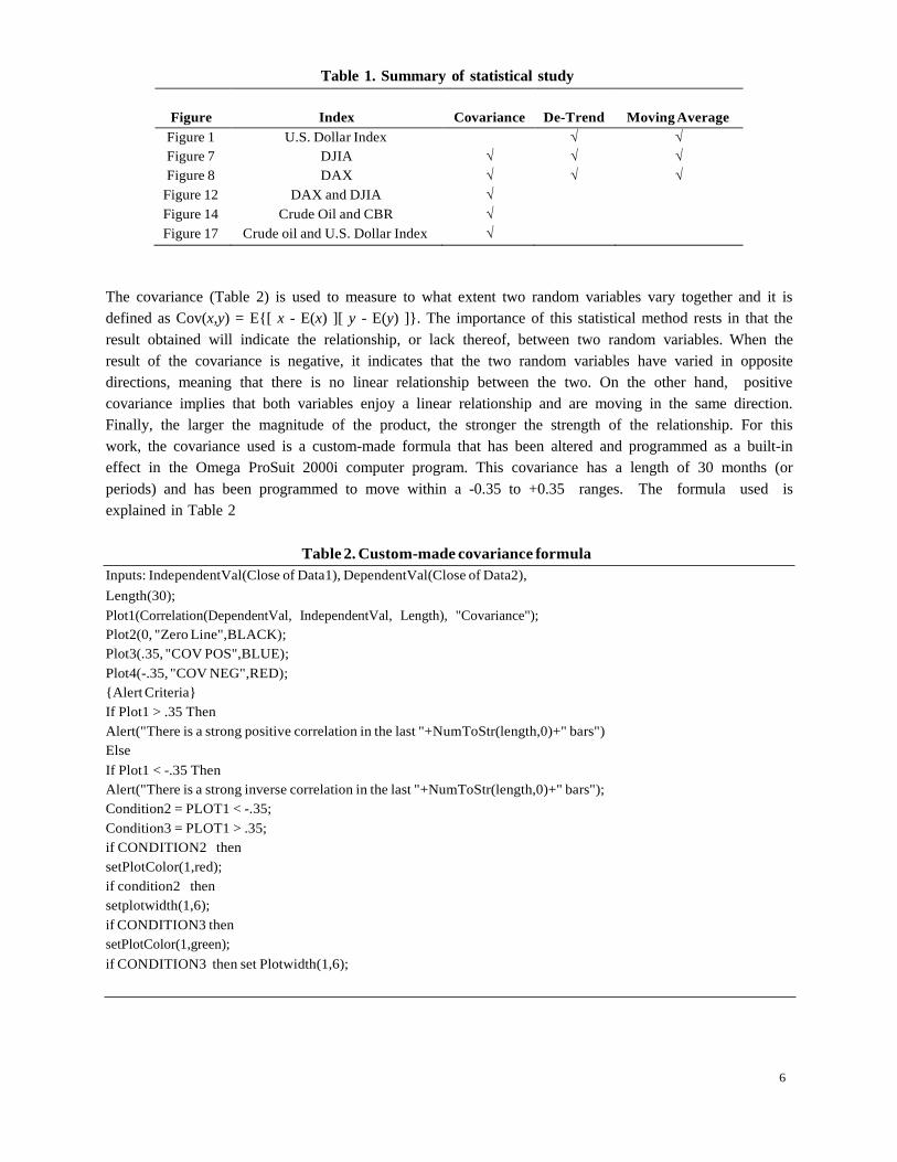
Table 1. Summary of statistical study

Figure

Index

Covariance

De-Trend

Moving Average

Figure 1 U.S. Dollar Index √ √ Figure 7 DJIA √ √ √ Figure 8 DAX √ √ √

Figure 12 DAX and DJIA √ Figure 14 Crude Oil and CBR √ Figure 17 Crude oil and U.S. Dollar Index √

The covariance (Table 2) is used to measure to what extent two random variables vary together and it is defined as Cov(x,y) = E{[ x - E(x) ][ y - E(y) ]}. The importance of this statistical method rests in that the result obtained will indicate the relationship, or lack thereof, between two random variables. When the result of the covariance is negative, it indicates that the two random variables have varied in opposite directions, meaning that there is no linear relationship between the two. On the other hand, positive covariance implies that both variables enjoy a linear relationship and are moving in the same direction. Finally, the larger the magnitude of the product, the stronger the strength of the relationship. For this work, the covariance used is a custom-made formula that has been altered and programmed as a built-in effect in the Omega ProSuit 2000i computer program. This covariance has a length of 30 months (or periods) and has been programmed to move within a -0.35 to +0.35 ranges. The formula used is explained in Table 2

Table 2. Custom-made covariance formula

Inputs: IndependentVal(Close of Data1), DependentVal(Close of Data2), Length(30); Plot1(Correlation(DependentVal, IndependentVal, Length), "Covariance"); Plot2(0, "Zero Line",BLACK); Plot3(.35, "COV POS",BLUE); Plot4(-.35, "COV NEG",RED); {Alert Criteria} If Plot1 > .35 Then Alert("There is a strong positive correlation in the last "+NumToStr(length,0)+" bars") Else If Plot1 < -.35 Then Alert("There is a strong inverse correlation in the last "+NumToStr(length,0)+" bars"); Condition2 = PLOT1 < -.35; Condition3 = PLOT1 > .35; if CONDITION2 then setPlotColor(1,red); if condition2 then setplotwidth(1,6); if CONDITION3 then setPlotColor(1,green); if CONDITION3 then set Plotwidth(1,6);

6

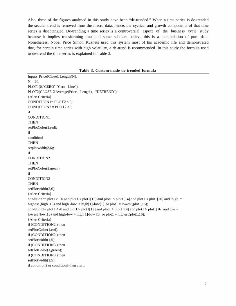
Also, three of the figures analysed in this study have been “de-trended.” When a time series is de-trended the secular trend is removed from the macro data, hence, the cyclical and growth components of that time series is disentangled. De-trending a time series is a controversial aspect of the business cycle study because it implies transforming data and some scholars believe this is a manipulation of pure data. Nonetheless, Nobel Price Simon Kuznets used this system most of his academic life and demonstrated that, for certain time series with high volatility, a de-trend is recommended. In this study the formula used to de-trend the time series is explained in Table 3.

Inputs: Price(Close), Length(N); N = 20;

Table 3. Custom-made de-trended formula

PLOT1(0,"CERO",”Cero Line”); PLOT2(CLOSE-XAverage(Price, Length), "DETREND"); {Alert Criteria} CONDITION1= PLOT2 < 0; CONDITION2 = PLOT2 >0; if CONDITION1 THEN setPlotColor(2,red); if condition1 THEN setplotwidth(2,6); if CONDITION2 THEN setPlotColor(2,green); if CONDITION2 THEN setPlotwidth(2,6); {Alert Criteria} condition2= plot1 > +0 and plot1 < plot1[12] and plot1 < plot1[14] and plot1 < plot1[16] and high = highest (high ,16) and high -low > high[1]-low[1] or plot1 = lowest(plot1,16); condition3= plot1 < -0 and plot1 > plot1[12] and plot1 > plot1[14] and plot1 > plot1[16] and low = lowest (low,16) and high-low > high[1]-low [1] or plot1 = highest(plot1,16); {Alert Criteria} if (CONDITION2 ) then setPlotColor(1,red); if (CONDITION2 ) then setPlotwidth(1,5); if (CONDITION3 ) then setPlotColor(1,green); if (CONDITION3 ) then setPlotwidth(1,5); if condition2 or condition3 then alert;

7

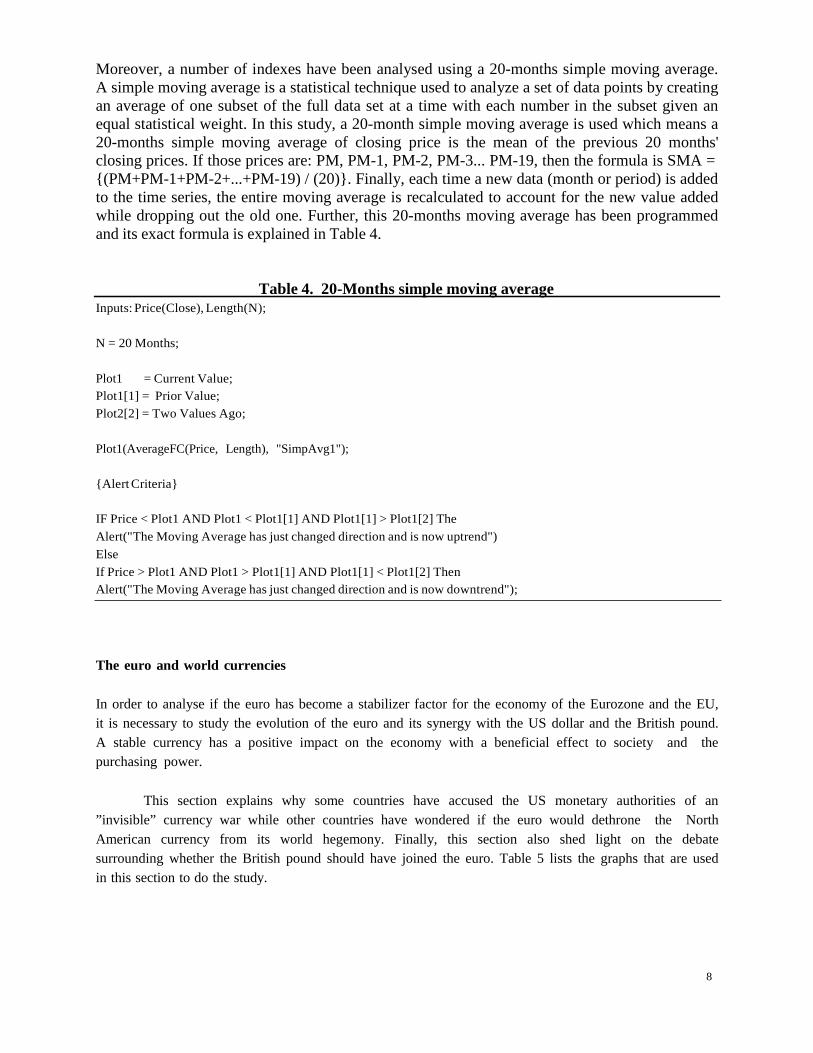
Moreover, a number of indexes have been analysed using a 20-months simple moving average. A simple moving average is a statistical technique used to analyze a set of data points by creating an average of one subset of the full data set at a time with each number in the subset given an equal statistical weight. In this study, a 20-month simple moving average is used which means a 20-months simple moving average of closing price is the mean of the previous 20 months' closing prices. If those prices are: PM, PM-1, PM-2, PM-3... PM-19, then the formula is SMA = {(PM+PM-1+PM-2+...+PM-19) / (20)}. Finally, each time a new data (month or period) is added to the time series, the entire moving average is recalculated to account for the new value added while dropping out the old one. Further, this 20-months moving average has been programmed and its exact formula is explained in Table 4.

Table 4. 20-Months simple moving average Inputs: Price(Close), Length(N);

N = 20 Months;

Plot1 = Current Value; Plot1[1] = Prior Value; Plot2[2] = Two Values Ago;

Plot1(AverageFC(Price, Length), "SimpAvg1");

{Alert Criteria}

IF Price < Plot1 AND Plot1 < Plot1[1] AND Plot1[1] > Plot1[2] The Alert("The Moving Average has just changed direction and is now uptrend") Else If Price > Plot1 AND Plot1 > Plot1[1] AND Plot1[1] < Plot1[2] Then Alert("The Moving Average has just changed direction and is now downtrend");

The euro and world currencies

In order to analyse if the euro has become a stabilizer factor for the economy of the Eurozone and the EU, it is necessary to study the evolution of the euro and its synergy with the US dollar and the British pound. A stable currency has a positive impact on the economy with a beneficial effect to society and the purchasing power.

This section explains why some countries have accused the US monetary authorities of an

”invisible” currency war while other countries have wondered if the euro would dethrone the North American currency from its world hegemony. Finally, this section also shed light on the debate surrounding whether the British pound should have joined the euro. Table 5 lists the graphs that are used in this section to do the study.

8

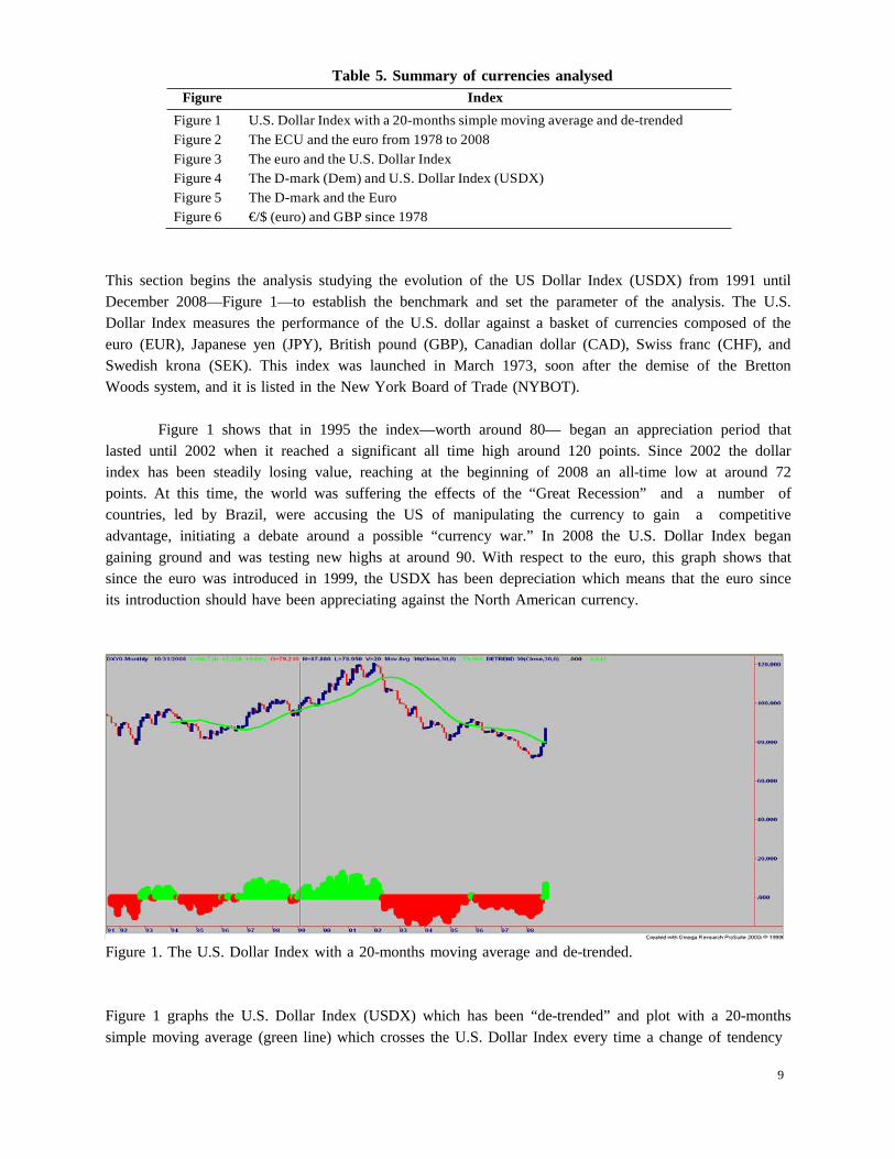
Table 5. Summary of currencies analysed

Figure Index

Figure 1 U.S. Dollar Index with a 20-months simple moving average and de-trended Figure 2 The ECU and the euro from 1978 to 2008 Figure 3 The euro and the U.S. Dollar Index Figure 4 The D-mark (Dem) and U.S. Dollar Index (USDX) Figure 5 The D-mark and the Euro Figure 6 €/$ (euro) and GBP since 1978

This section begins the analysis studying the evolution of the US Dollar Index (USDX) from 1991 until December 2008—Figure 1—to establish the benchmark and set the parameter of the analysis. The U.S. Dollar Index measures the performance of the U.S. dollar against a basket of currencies composed of the euro (EUR), Japanese yen (JPY), British pound (GBP), Canadian dollar (CAD), Swiss franc (CHF), and Swedish krona (SEK). This index was launched in March 1973, soon after the demise of the Bretton Woods system, and it is listed in the New York Board of Trade (NYBOT).

Figure 1 shows that in 1995 the index—worth around 80— began an appreciation period that

lasted until 2002 when it reached a significant all time high around 120 points. Since 2002 the dollar index has been steadily losing value, reaching at the beginning of 2008 an all-time low at around 72 points. At this time, the world was suffering the effects of the “Great Recession” and a number of countries, led by Brazil, were accusing the US of manipulating the currency to gain a competitive advantage, initiating a debate around a possible “currency war.” In 2008 the U.S. Dollar Index began gaining ground and was testing new highs at around 90. With respect to the euro, this graph shows that since the euro was introduced in 1999, the USDX has been depreciation which means that the euro since its introduction should have been appreciating against the North American currency.

Figure 1. The U.S. Dollar Index with a 20-months moving average and de-trended.

Figure 1 graphs the U.S. Dollar Index (USDX) which has been “de-trended” and plot with a 20-months simple moving average (green line) which crosses the U.S. Dollar Index every time a change of tendency

9

is taking place. This change of tendency is further corroborated by the “de-trend” of the index, which, when the index is changing tendency and is going up, the de-trend is in green and when the index changes tendency and is losing value, the de-trend is in red.

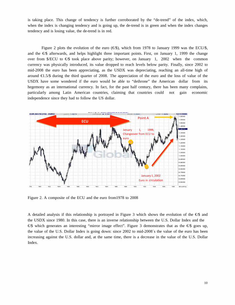
Figure 2 plots the evolution of the euro (€/$), which from 1978 to January 1999 was the ECU/$, and the €/$ afterwards, and helps highlight three important points. First, on January 1, 1999 the change over from $/ECU to €/$ took place above parity; however, on January 1, 2002 when the common currency was physically introduced, its value dropped to reach levels below parity. Finally, since 2002 to mid-2008 the euro has been appreciating, as the USDX was depreciating, reaching an all-time high of around €1.5/$ during the third quarter of 2008. The appreciation of the euro and the loss of value of the USDX have some wondered if the euro would be able to “dethrone” the American dollar from its hegemony as an international currency. In fact, for the past half century, there has been many complains, particularly among Latin American countries, claiming that countries could not gain economic independence since they had to follow the US dollar.

Figure 2. A composite of the ECU and the euro from1978 to 2008

A detailed analysis if this relationship is portrayed in Figure 3 which shows the evolution of the €/$ and the USDX since 1980. In this case, there is an inverse relationship between the U.S. Dollar Index and the €/$ which generates an interesting “mirror image effect”. Figure 3 demonstrates that as the €/$ goes up, the value of the U.S. Dollar Index is going down: since 2002 to mid-2008´s the value of the euro has been increasing against the U.S. dollar and, at the same time, there is a decrease in the value of the U.S. Dollar Index.

Point A ECU

January 1, 1999, Changeover from ECU to euro

January 1, 2002 Euro in circulation

10

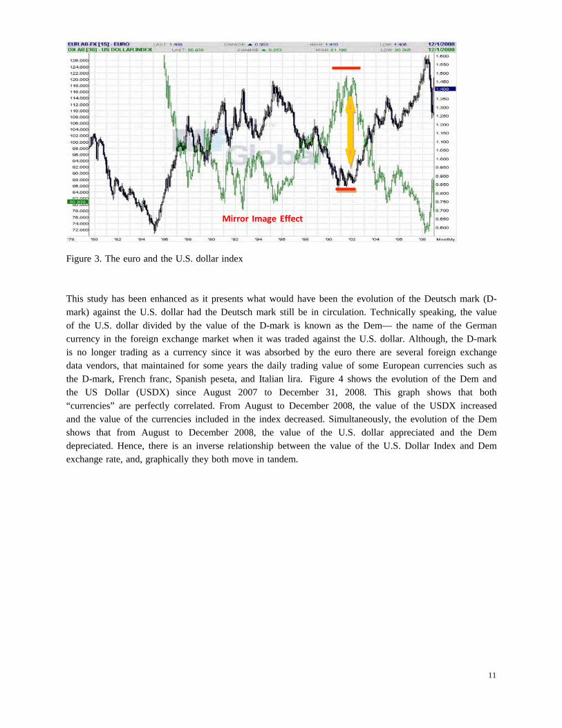
Figure 3. The euro and the U.S. dollar index

This study has been enhanced as it presents what would have been the evolution of the Deutsch mark (D- mark) against the U.S. dollar had the Deutsch mark still be in circulation. Technically speaking, the value of the U.S. dollar divided by the value of the D-mark is known as the Dem— the name of the German currency in the foreign exchange market when it was traded against the U.S. dollar. Although, the D-mark is no longer trading as a currency since it was absorbed by the euro there are several foreign exchange data vendors, that maintained for some years the daily trading value of some European currencies such as the D-mark, French franc, Spanish peseta, and Italian lira. Figure 4 shows the evolution of the Dem and the US Dollar (USDX) since August 2007 to December 31, 2008. This graph shows that both “currencies” are perfectly correlated. From August to December 2008, the value of the USDX increased and the value of the currencies included in the index decreased. Simultaneously, the evolution of the Dem shows that from August to December 2008, the value of the U.S. dollar appreciated and the Dem depreciated. Hence, there is an inverse relationship between the value of the U.S. Dollar Index and Dem exchange rate, and, graphically they both move in tandem.

Mirror Image Effect

11

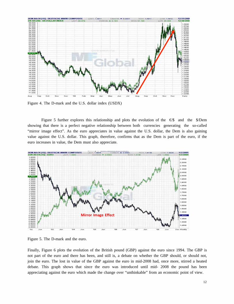
Figure 4. The D-mark and the U.S. dollar index (USDX)

Figure 5 further explores this relationship and plots the evolution of the €/$ and the $/Dem showing that there is a perfect negative relationship between both currencies generating the so-called “mirror image effect”. As the euro appreciates in value against the U.S. dollar, the Dem is also gaining value against the U.S. dollar. This graph, therefore, confirms that as the Dem is part of the euro, if the euro increases in value, the Dem must also appreciate.

Figure 5. The D-mark and the euro.

Finally, Figure 6 plots the evolution of the British pound (GBP) against the euro since 1994. The GBP is not part of the euro and there has been, and still is, a debate on whether the GBP should, or should not, join the euro. The lost in value of the GBP against the euro in mid-2008 had, once more, stirred a heated debate. This graph shows that since the euro was introduced until mid- 2008 the pound has been appreciating against the euro which made the change over “unthinkable” from an economic point of view.

Mirror Image Effect

12

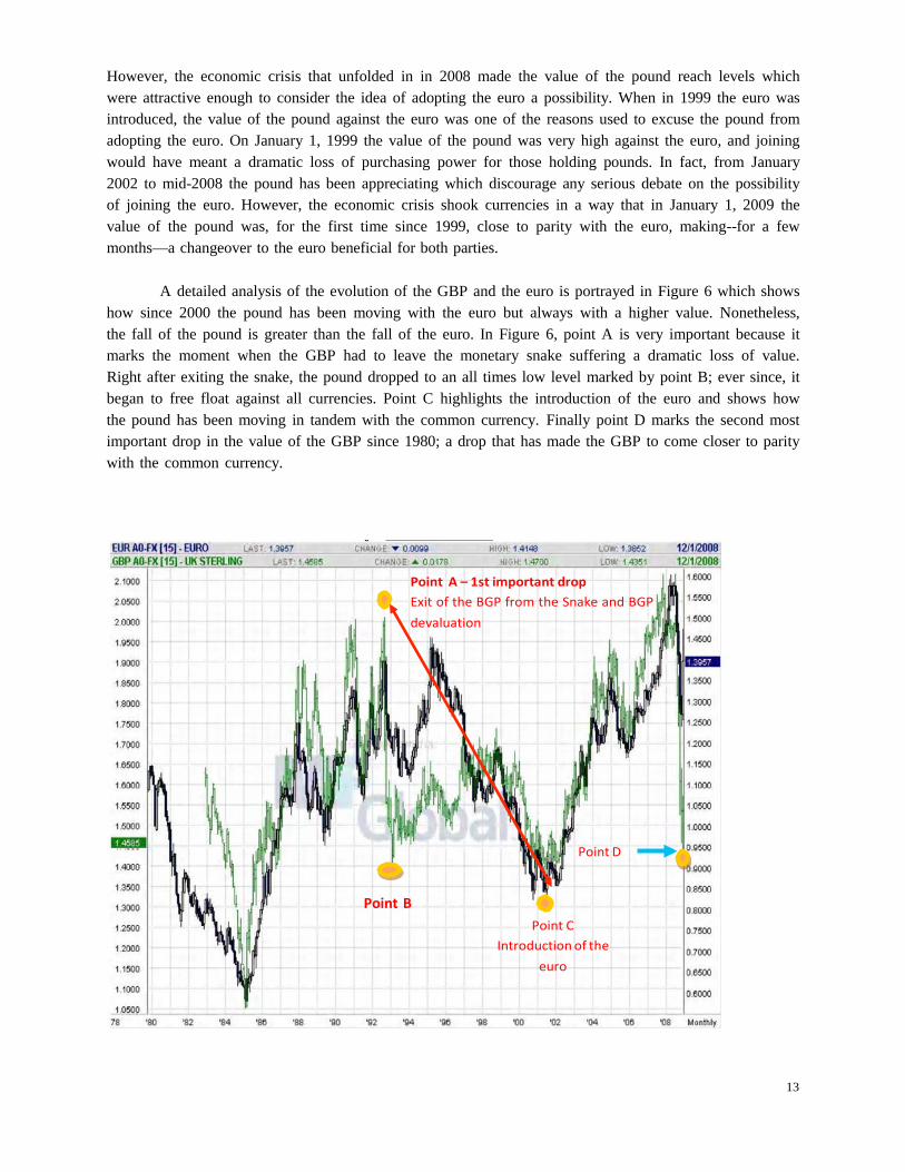
However, the economic crisis that unfolded in in 2008 made the value of the pound reach levels which were attractive enough to consider the idea of adopting the euro a possibility. When in 1999 the euro was introduced, the value of the pound against the euro was one of the reasons used to excuse the pound from adopting the euro. On January 1, 1999 the value of the pound was very high against the euro, and joining would have meant a dramatic loss of purchasing power for those holding pounds. In fact, from January 2002 to mid-2008 the pound has been appreciating which discourage any serious debate on the possibility of joining the euro. However, the economic crisis shook currencies in a way that in January 1, 2009 the value of the pound was, for the first time since 1999, close to parity with the euro, making--for a few months—a changeover to the euro beneficial for both parties.

A detailed analysis of the evolution of the GBP and the euro is portrayed in Figure 6 which shows

how since 2000 the pound has been moving with the euro but always with a higher value. Nonetheless, the fall of the pound is greater than the fall of the euro. In Figure 6, point A is very important because it marks the moment when the GBP had to leave the monetary snake suffering a dramatic loss of value. Right after exiting the snake, the pound dropped to an all times low level marked by point B; ever since, it began to free float against all currencies. Point C highlights the introduction of the euro and shows how the pound has been moving in tandem with the common currency. Finally point D marks the second most important drop in the value of the GBP since 1980; a drop that has made the GBP to come closer to parity with the common currency.

Point A – 1st important drop Exit of the BGP from the Snake and BGP devaluation

Point D

Point B Point C

Introduction of the euro

13

Figure 6. The GBP and the euro since 1978 In summary, Figures 1 through 6 have brought across four interesting points. First, this work plots the evolution of the Deutsch mark that do not exist anymore however her trading values are still published by Future Source. This confirms the fact that the euro is basically the continuation of the Dem, and that there is perfect inverse relation between the euro and the Dem against the U.S. Dollar Index. Thirdly, it has been shown that that the euro, as well as all the currencies that form it, have been moving together, providing the euro with strength and stability. Finally, it can be concluded that the euro stabilized the value of the British pound, bringing it to a level which, for the first time in history, made jumping on- board the “euro boat” interesting for the British economy.

14

The euro and world indexes The second section of this study analyses whether the euro has become a stabilizing factor for the Eurozone evaluating if the euro has helped smooth the business cycle measured by the correlation between the euro and the Dow Jones Industrial Average (DJIA), the German Deutscher Aktien IndeX 30 (DAX), the CRB Index, and Light Crude oil price. Table 6 presents a summary of all the indexes analyzed in this section and the statistical method used to better understand their behaviour.

Table 6. Summary of stock exchange indexes, Crude oil, and CRB.

Figure Index

Figure 7 DJIA with 20-months moving averaged and de-trend Figure 8 DAX and 30-months moving average and de-trend Figure 9 DJIA and U.S. Dollar Index since 1978 Figure 10 DAX and euro since 1978 Figure 11 DAX and DJIA Figure 12 DAX and DJIA with covariance Figure 13 Crude Oil and CRB since 2002 Figure 14 Crude Oil and CRB with covariance Figure 15 CRB and U.S. Dollar Index Figure 16 Crude Oil and U.S. Dollar Index Figure 17 Crude Oil and U.S. Dollar Index with covariance Figure 18 Crude Oil and euro (€/$)

Figure 7 graphs the evolution of the Dow Jones Industrial Average (DJIA) from 1984 to January 1, 2009. The DJIA measures since 1896 the daily performance of 30 of the largest ‘blue-chip’ corporations in the United States, making the DJIA the best-known measure of the performance of the stock market in the United States. The DJIA is traded in the New York Stock Exchange (NYSE) in U.S. dollars. Figure 7 shows that in mid-2007 the DJIA reached an all-time high around 1,400 points after which it began to lose value to reach levels of around 7,500 points—levels tested in 2002 and 2004. Figure 7 studies the DJIA when measured with an optimized 30-months moving average and the de-trend of the index. This Figure shows that when the moving average crosses the index a change of tendency follows. This change of tendency is supported by the de-trend because every time the moving average crosses the DJIA, a change of tendency follows and the de-trend simultaneously changes. This figures demonstrates the validity of a 30-months moving average to forecast a change in tendency when plotted with the DJIA.

15

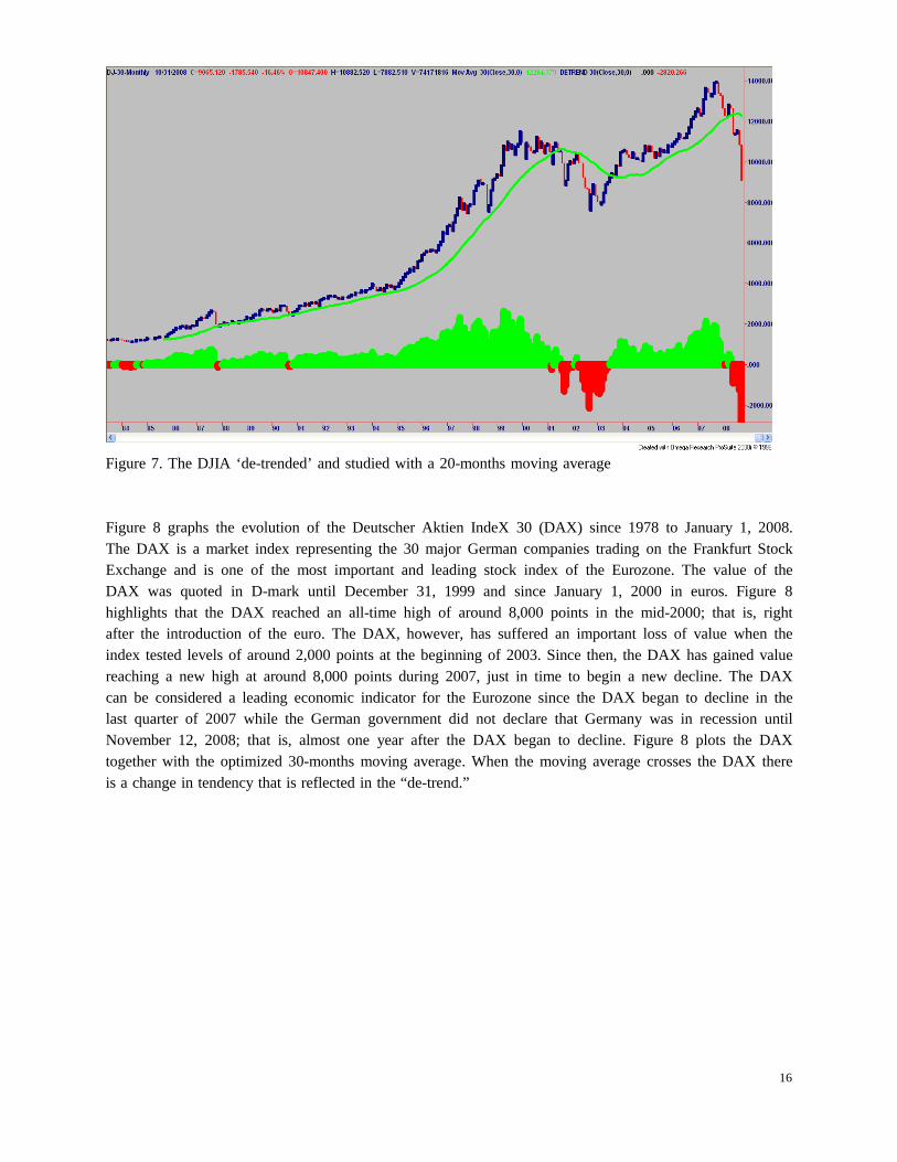
Figure 7. The DJIA ‘de-trended’ and studied with a 20-months moving average

Figure 8 graphs the evolution of the Deutscher Aktien IndeX 30 (DAX) since 1978 to January 1, 2008. The DAX is a market index representing the 30 major German companies trading on the Frankfurt Stock Exchange and is one of the most important and leading stock index of the Eurozone. The value of the DAX was quoted in D-mark until December 31, 1999 and since January 1, 2000 in euros. Figure 8 highlights that the DAX reached an all-time high of around 8,000 points in the mid-2000; that is, right after the introduction of the euro. The DAX, however, has suffered an important loss of value when the index tested levels of around 2,000 points at the beginning of 2003. Since then, the DAX has gained value reaching a new high at around 8,000 points during 2007, just in time to begin a new decline. The DAX can be considered a leading economic indicator for the Eurozone since the DAX began to decline in the last quarter of 2007 while the German government did not declare that Germany was in recession until November 12, 2008; that is, almost one year after the DAX began to decline. Figure 8 plots the DAX together with the optimized 30-months moving average. When the moving average crosses the DAX there is a change in tendency that is reflected in the “de-trend.”

16

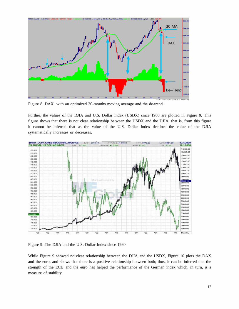
Figure 8. DAX with an optimized 30-months moving average and the de-trend

Further, the values of the DJIA and U.S. Dollar Index (USDX) since 1980 are plotted in Figure 9. This figure shows that there is not clear relationship between the USDX and the DJIA; that is, from this figure it cannot be inferred that as the value of the U.S. Dollar Index declines the value of the DJIA systematically increases or decreases.

Figure 9. The DJIA and the U.S. Dollar Index since 1980

While Figure 9 showed no clear relationship between the DJIA and the USDX, Figure 10 plots the DAX and the euro, and shows that there is a positive relationship between both; thus, it can be inferred that the strength of the ECU and the euro has helped the performance of the German index which, in turn, is a measure of stability.

30 MA

DAX

De---Trend

17

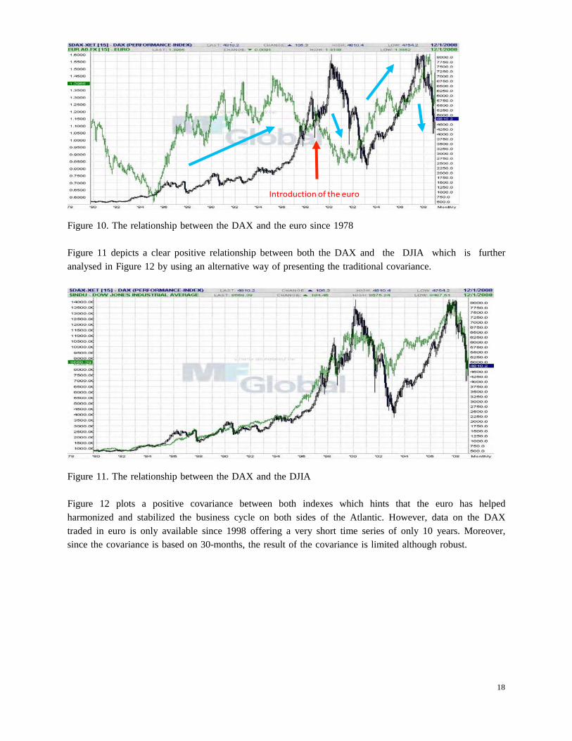
Figure 10. The relationship between the DAX and the euro since 1978

Figure 11 depicts a clear positive relationship between both the DAX and the DJIA which is further analysed in Figure 12 by using an alternative way of presenting the traditional covariance.

Figure 11. The relationship between the DAX and the DJIA

Figure 12 plots a positive covariance between both indexes which hints that the euro has helped harmonized and stabilized the business cycle on both sides of the Atlantic. However, data on the DAX traded in euro is only available since 1998 offering a very short time series of only 10 years. Moreover, since the covariance is based on 30-months, the result of the covariance is limited although robust.

Introduction of the euro

18

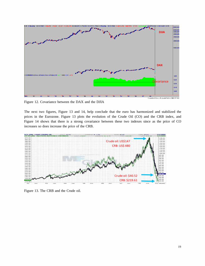
Figure 12. Covariance between the DAX and the DJIA

The next two figures, Figure 13 and 14, help conclude that the euro has harmonized and stabilized the prices in the Eurozone. Figure 13 plots the evolution of the Crude Oil (CO) and the CRB index, and Figure 14 shows that there is a strong covariance between these two indexes since as the price of CO increases so does increase the price of the CRB.

Figure 13. The CRB and the Crude oil.

Crude oil: US$147 CRB: US$ 480

Crude oil: $40.52 CRB: $219.61

DJIA

DAX

Covariance

19

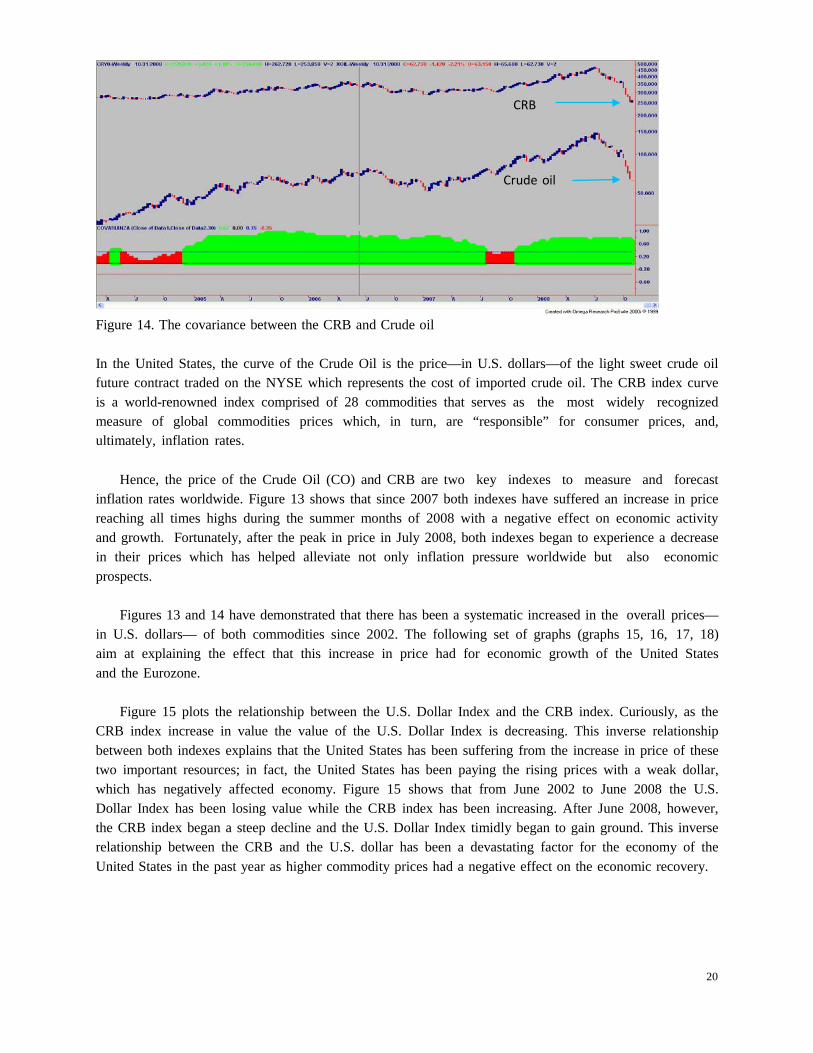
Figure 14. The covariance between the CRB and Crude oil

In the United States, the curve of the Crude Oil is the price—in U.S. dollars—of the light sweet crude oil future contract traded on the NYSE which represents the cost of imported crude oil. The CRB index curve is a world-renowned index comprised of 28 commodities that serves as the most widely recognized measure of global commodities prices which, in turn, are “responsible” for consumer prices, and, ultimately, inflation rates.

Hence, the price of the Crude Oil (CO) and CRB are two key indexes to measure and forecast

inflation rates worldwide. Figure 13 shows that since 2007 both indexes have suffered an increase in price reaching all times highs during the summer months of 2008 with a negative effect on economic activity and growth. Fortunately, after the peak in price in July 2008, both indexes began to experience a decrease in their prices which has helped alleviate not only inflation pressure worldwide but also economic prospects.

Figures 13 and 14 have demonstrated that there has been a systematic increased in the overall prices—

in U.S. dollars— of both commodities since 2002. The following set of graphs (graphs 15, 16, 17, 18) aim at explaining the effect that this increase in price had for economic growth of the United States and the Eurozone.

Figure 15 plots the relationship between the U.S. Dollar Index and the CRB index. Curiously, as the

CRB index increase in value the value of the U.S. Dollar Index is decreasing. This inverse relationship between both indexes explains that the United States has been suffering from the increase in price of these two important resources; in fact, the United States has been paying the rising prices with a weak dollar, which has negatively affected economy. Figure 15 shows that from June 2002 to June 2008 the U.S. Dollar Index has been losing value while the CRB index has been increasing. After June 2008, however, the CRB index began a steep decline and the U.S. Dollar Index timidly began to gain ground. This inverse relationship between the CRB and the U.S. dollar has been a devastating factor for the economy of the United States in the past year as higher commodity prices had a negative effect on the economic recovery.

CRB

Crude oil

20

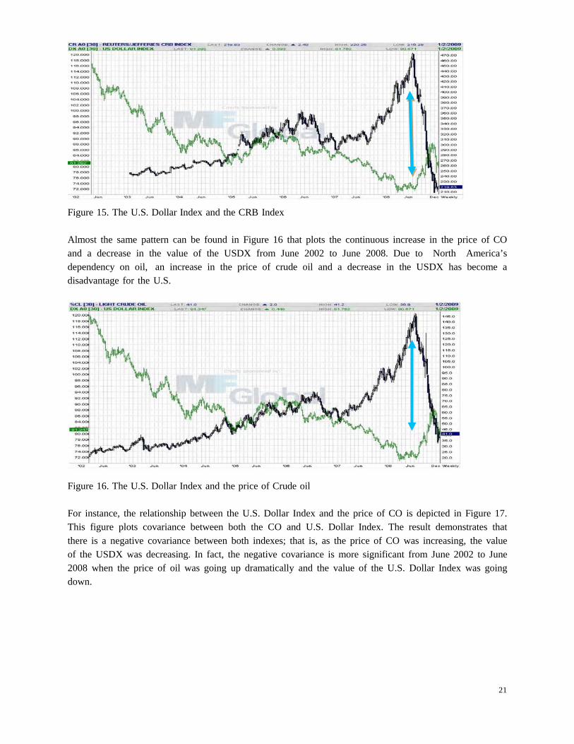
Figure 15. The U.S. Dollar Index and the CRB Index

Almost the same pattern can be found in Figure 16 that plots the continuous increase in the price of CO and a decrease in the value of the USDX from June 2002 to June 2008. Due to North America’s dependency on oil, an increase in the price of crude oil and a decrease in the USDX has become a disadvantage for the U.S.

Figure 16. The U.S. Dollar Index and the price of Crude oil

For instance, the relationship between the U.S. Dollar Index and the price of CO is depicted in Figure 17. This figure plots covariance between both the CO and U.S. Dollar Index. The result demonstrates that there is a negative covariance between both indexes; that is, as the price of CO was increasing, the value of the USDX was decreasing. In fact, the negative covariance is more significant from June 2002 to June 2008 when the price of oil was going up dramatically and the value of the U.S. Dollar Index was going down.

21

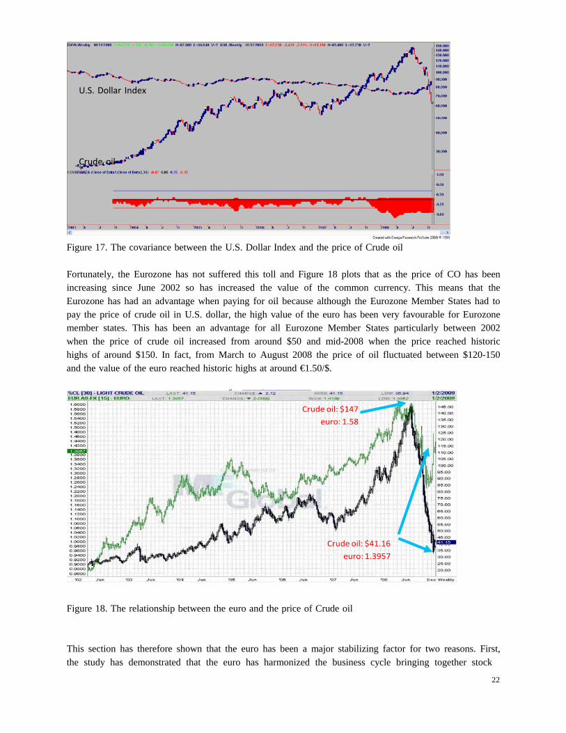
Figure 17. The covariance between the U.S. Dollar Index and the price of Crude oil

Fortunately, the Eurozone has not suffered this toll and Figure 18 plots that as the price of CO has been increasing since June 2002 so has increased the value of the common currency. This means that the Eurozone has had an advantage when paying for oil because although the Eurozone Member States had to pay the price of crude oil in U.S. dollar, the high value of the euro has been very favourable for Eurozone member states. This has been an advantage for all Eurozone Member States particularly between 2002 when the price of crude oil increased from around $50 and mid-2008 when the price reached historic highs of around $150. In fact, from March to August 2008 the price of oil fluctuated between $120-150 and the value of the euro reached historic highs at around €1.50/$.

Figure 18. The relationship between the euro and the price of Crude oil

This section has therefore shown that the euro has been a major stabilizing factor for two reasons. First, the study has demonstrated that the euro has harmonized the business cycle bringing together stock

Crude oil: $147 euro: 1.58

Crude oil: $41.16 euro: 1.3957

U.S. Dollar Index

Crude oil

22

indexes prices which are considered leading economic indicator. Second, the strong euro has helped pay the high prices of crude oil and commodities in the Eurozone which, in turn, has helped maintained inflation under control.

The euro and money market indexes

This section analyses Figures 19 through 27 to study the relationship between the euro and the Money Market (MM). The MM is a subsector of the fixed-income market and consists of very short-term debt securities that usually are highly marketable. Analysing the MM is important because the ECB uses the MM as escape valve to fight inflation and to maintain price stability. Whatever decision the ECB takes to fight inflation and maintain stability will, in turn, affect the value of the euro. Moreover, understanding MM in the U.S. sets the ground to understand the MM in the Eurozone. Table 6 presents the list of the graphs used for this analysis.

Table 3. Summary of money market indexes

Figure Index

Figure 19 Treasury Note 2-years and Eurodollar 3-months Figure 20 Treasury Note 10-years and the German Bund Figure 21 €/$ and German Bund Figure 22 LIBOR 1-month and Eurodollar 3-months Figure 23 EURIBOR 3-months and Eurodollar 3-months Figure 24 EURIBOR 3-months and LIBOR 1-month Figure 25 EURIBOR 3-months and €/$ Figure 26 U.S. Consumer Price Index Figure 27 Euro Area HICP

Figure 19 plots both the U.S. 2-years Treasury Note (T-Note) and the Eurodollar. The Eurodollar is the name given to all the dollar-denominated deposits at foreign banks, or foreign branches, of American banks. Despite the tag “euro”, these deposits are not in euros. Most Eurodollar deposits are for large sums with less than six months maturity. Based on these deposits, the Eurodollar futures contracts are futures contracts traded at the Chicago Mercantile Exchange (CME) in Chicago. U.S. 2-years T-Note is a U.S. government debt financing instrument issued by the U.S. Department of the Treasury. Figure 19 shows that both index move in unison although it seems as if the 2-years T-Note could lead changes in tendency.

23

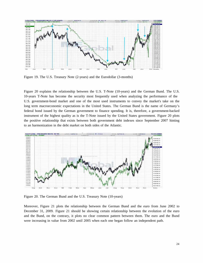
Figure 19. The U.S. Treasury Note (2-years) and the Eurodollar (3-months)

Figure 20 explains the relationship between the U.S. T-Note (10-years) and the German Bund. The U.S. 10-years T-Note has become the security most frequently used when analyzing the performance of the U.S. government-bond market and one of the most used instruments to convey the market's take on the long term macroeconomic expectations in the United States. The German Bund is the name of Germany’s federal bond issued by the German government to finance spending. It is, therefore, a government-backed instrument of the highest quality as is the T-Note issued by the United States government. Figure 20 plots the positive relationship that exists between both government debt indexes since September 2007 hinting to an harmonization in the debt market on both sides of the Atlantic.

Figure 20. The German Bund and the U.S. Treasury Note (10-years)

Moreover, Figure 21 plots the relationship between the German Bund and the euro from June 2002 to December 31, 2009. Figure 21 should be showing certain relationship between the evolution of the euro and the Bund, on the contrary, it plots no clear common pattern between them. The euro and the Bund were increasing in value from 2002 until 2005 when each one began follow an independent path.

24

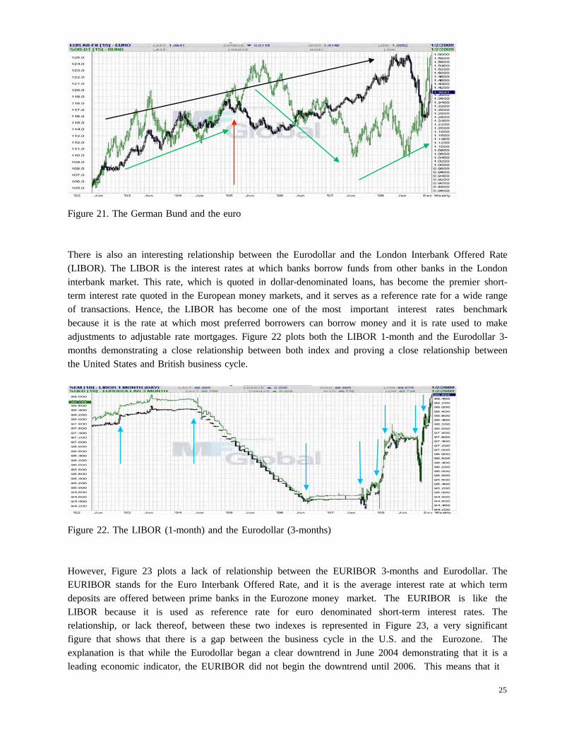
Figure 21. The German Bund and the euro

There is also an interesting relationship between the Eurodollar and the London Interbank Offered Rate (LIBOR). The LIBOR is the interest rates at which banks borrow funds from other banks in the London interbank market. This rate, which is quoted in dollar-denominated loans, has become the premier short- term interest rate quoted in the European money markets, and it serves as a reference rate for a wide range of transactions. Hence, the LIBOR has become one of the most important interest rates benchmark because it is the rate at which most preferred borrowers can borrow money and it is rate used to make adjustments to adjustable rate mortgages. Figure 22 plots both the LIBOR 1-month and the Eurodollar 3- months demonstrating a close relationship between both index and proving a close relationship between the United States and British business cycle.

Figure 22. The LIBOR (1-month) and the Eurodollar (3-months)

However, Figure 23 plots a lack of relationship between the EURIBOR 3-months and Eurodollar. The EURIBOR stands for the Euro Interbank Offered Rate, and it is the average interest rate at which term deposits are offered between prime banks in the Eurozone money market. The EURIBOR is like the LIBOR because it is used as reference rate for euro denominated short-term interest rates. The relationship, or lack thereof, between these two indexes is represented in Figure 23, a very significant figure that shows that there is a gap between the business cycle in the U.S. and the Eurozone. The explanation is that while the Eurodollar began a clear downtrend in June 2004 demonstrating that it is a leading economic indicator, the EURIBOR did not begin the downtrend until 2006. This means that it

25

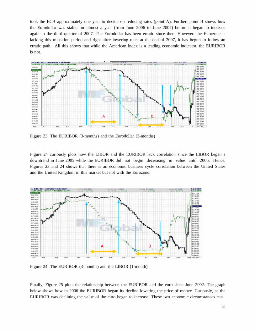
took the ECB approximately one year to decide on reducing rates (point A). Further, point B shows how the Eurodollar was stable for almost a year (from June 2006 to June 2007) before it began to increase again in the third quarter of 2007. The Eurodollar has been erratic since then. However, the Eurozone is lacking this transition period and right after lowering rates at the end of 2007, it has begun to follow an erratic path. All this shows that while the American index is a leading economic indicator, the EURIBOR is not.

Figure 23. The EURIBOR (3-months) and the Eurodollar (3-months)

Figure 24 curiously plots how the LIBOR and the EURIBOR lack correlation since the LIBOR began a downtrend in June 2005 while the EURIBOR did not begin decreasing in value until 2006. Hence, Figures 23 and 24 shows that there is an economic business cycle correlation between the United States and the United Kingdom in this market but not with the Eurozone.

Figure 24. The EURIBOR (3-months) and the LIBOR (1-month)

Finally, Figure 25 plots the relationship between the EURIBOR and the euro since June 2002. The graph below shows how in 2006 the EURIBOR began its decline lowering the price of money. Curiously, as the EURIBOR was declining the value of the euro began to increase. These two economic circumstances can

A B

A B

26

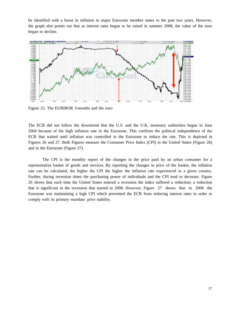
be identified with a boost in inflation in major Eurozone member states in the past two years. However, the graph also points out that as interest rates began to be raised in summer 2008, the value of the euro began to decline.

Figure 25. The EURIBOR 3-months and the euro

The ECB did not follow the downtrend that the U.S. and the U.K. monetary authorities began in June 2004 because of the high inflation rate in the Eurozone. This confirms the political independence of the ECB that waited until inflation was controlled in the Eurozone to reduce the rate. This is depicted in Figures 26 and 27. Both Figures measure the Consumer Price Index (CPI) in the United States (Figure 26) and in the Eurozone (Figure 27).

The CPI is the monthly report of the changes in the price paid by an urban consumer for a

representative basket of goods and services. By reporting the changes in price of the basket, the inflation rate can be calculated, the higher the CPI the higher the inflation rate experienced in a given country. Further, during recession times the purchasing power of individuals and the CPI tend to decrease. Figure 26 shows that each time the United States entered a recession the index suffered a reduction; a reduction that is significant in the recession that started in 2008. However, Figure 27 shows that in 2008 the Eurozone was maintaining a high CPI which prevented the ECB from reducing interest rates in order to comply with its primary mandate: price stability.

27

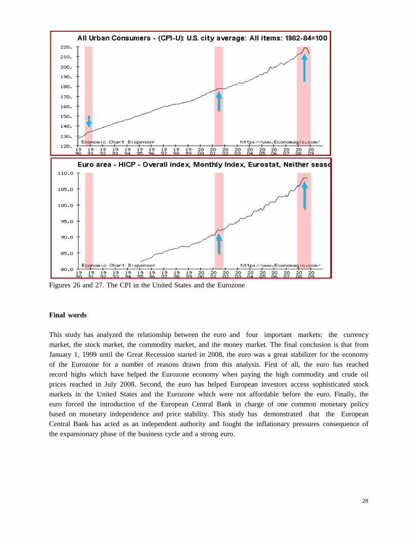
Figures 26 and 27. The CPI in the United States and the Eurozone

Final words

This study has analyzed the relationship between the euro and four important markets: the currency market, the stock market, the commodity market, and the money market. The final conclusion is that from January 1, 1999 until the Great Recession started in 2008, the euro was a great stabilizer for the economy of the Eurozone for a number of reasons drawn from this analysis. First of all, the euro has reached record highs which have helped the Eurozone economy when paying the high commodity and crude oil prices reached in July 2008. Second, the euro has helped European investors access sophisticated stock markets in the United States and the Eurozone which were not affordable before the euro. Finally, the euro forced the introduction of the European Central Bank in charge of one common monetary policy based on monetary independence and price stability. This study has demonstrated that the European Central Bank has acted as an independent authority and fought the inflationary pressures consequence of the expansionary phase of the business cycle and a strong euro.

28

Work cited

Bergsten, Fred C. 2005. The dollar and the euro. In The global economy: Contemporary debates., ed. Thomas Oatley, 278-289. New York: Pearson Longman.

———. 2005. The euro and the dollar: Toward a ´Finance G-2´? In The euro at five: Ready for a global

role?, ed. Adam S. Posen. Vol. Special Report 18, 1-212 Institute for International Economics.

———. 2004. The euro versus the dollar: Will there be a struggle for dominance? Foreign Affairs 76, (4).

Doyle, Diane. Eurosclerosis revisited. Strategy and Business. Summer 2005, http://www.strategy- business.com/press/article/05210?gko=5eb5c-1876-9229626

European Commission. 2008. EMU @10: Successes and challenges after 10 years of economic and

monetary union. European Economy 2 Feldstein, Martin. March 3, 2006. The case for a competitive dollar. Remarks at the Annual SIEPR

Summit, Stanford University. ———. 2006. Europe has to face the threat of American's trade deficit. Financial Times, August 2 2006,

2006. ———. 2005. The euro and the stability pact. National Bureau of Economic Research WP 11249, (April

2005). ———. 2000. Europe can't handle the euro. The Wall Street Journal2000.

———. 2000. The European Central Bank and the euro: The first year. National Bureau of Economic

Research Working paper 7517. Kawai, Masahiro. 1997. Comments of Bergsten on Alogouskoufis and Portes. In EMU and the

international monetary system., ed. P. Masson, T. Krueger and B. Turtelboom. Washington: International Monetary Fund.

Levy, Mickey D. 2004. Ending Europe's economic underperformance. Cato Journal 24 (1/2): 71-4.

Mckinnon, Ronald I. 2004. Optimun currency areas and key currencies: Mundell I versus Mundell II. Journal of Common Markets 42 (4): 689-715.

Munchau, Wolfgang. 1999. Welcome to the euro-zone. Financial Times1999.

Mundell, Robert. March 24, 1998. The case for the euro - I and II. Wall Street Journal. March 24, 1998.

29

———. 23 October, 2003. The international monetary system and the case for a world currency. Paper presented at Leon Kozminski Academy of Entrepreneurship and management (WSPiZ) and TIGER, Distinguished Lecture Series n. 12, Warsaw.

Posen, Adam S. 2005. The euro at five: Ready for a global role?. Special report 18. Washington: Institute

for International Economics. Schwartz, Pedro. 2004. The euro as politics. Research monograph 58. London, UK: The Institute of

Economic Affairs. Skidelsky, Robert. The politics of euro economics. Financial Times, January 23, 2001.

30