Embed Size (px)
Citation preview
The Entropy of Musical Classification
A Thesis
Presented to
The Division of Mathematics and Natural Sciences
Reed College
In Partial Fulfillment
of the Requirements for the Degree
Bachelor of Arts
Regina E. Collecchia
May 2009

Approved for the Division(Mathematics)
Joe Roberts

Acknowledgements
Without the brilliant, almost computer-like minds of Noah Pepper, Dr. RichardCrandall, and Devin Chalmers, this thesis would absolutely not have been taken tothe levels I ambitiously intended it to go. Noah encouraged me to write about theunity of digitization and music in a way that made me completely enamored with mythesis throughout the entire length of the academic year. He introduced me to Dr.Crandall, whose many achievements made me see the working world in a more vividand compelling light. Then, Devin, a researcher for Richard, guided me through muchof the programming in Mathematica and C that was critical to a happy ending.
Most of all, however, I am indebted to Reed College for four years of wonder,and I am proud to say that I am very satisfied with myself for finding the clarity ofmind that the no-bullshit approach to academia helped me find, and allowed me toexpose a topic by which I am truly enthralled. I rarely find music boring, even whenI despise it, for my curiosity is always peaked by the emotions and concrete thoughtsit galvanizes and communicates. Yet, I doubt that I could have really believed thatI had the power to approach popular music in a sophisticated manner without theexcitement of my fellow Reedies and their nearly ubiquitous enthusiasm for music.This year more than any other has proven to me that there is no other place quitelike Reed, for me at least.
I would also like to thank my “wallmate” in Old Dorm Block for playing themost ridiculous pop music, not just once, but the same song 40 times consecutively,and thus weaseling me out of bed so many mornings; my parents, for ridiculousfinancial and increasing emotional support; Fourier and Euler, for some really elegantmathematics; the World Wide Web (as we used to call it in the dinosaur age knownas the nineties), for obvious reasons; and last but not least, Portland beer.

Table of Contents
Introduction . . . . . . . . . . . . . . . . . . . . . . . . . . . . . . . . . . . 1Motivations . . . . . . . . . . . . . . . . . . . . . . . . . . . . . . . . . . . 1
Why chord progressions? . . . . . . . . . . . . . . . . . . . . . . . . . 1Why digital filtering? . . . . . . . . . . . . . . . . . . . . . . . . . . . 2Why entropy? . . . . . . . . . . . . . . . . . . . . . . . . . . . . . . . 2Automatic Chord Recognition . . . . . . . . . . . . . . . . . . . . . . 3Smoothing . . . . . . . . . . . . . . . . . . . . . . . . . . . . . . . . . 3
Western Convention in Music . . . . . . . . . . . . . . . . . . . . . . . . . 4Procedure . . . . . . . . . . . . . . . . . . . . . . . . . . . . . . . . . . . . 6
Chapter 1: Automatic Recognition of Digital Audio Signals . . . . . 71.1 Digital Audio Signal Processing . . . . . . . . . . . . . . . . . . . . . 7
1.1.1 Sampling . . . . . . . . . . . . . . . . . . . . . . . . . . . . . 81.1.2 The Discrete Fourier Transform . . . . . . . . . . . . . . . . . 111.1.3 Properties of the Transform . . . . . . . . . . . . . . . . . . . 151.1.4 Filtering . . . . . . . . . . . . . . . . . . . . . . . . . . . . . . 17
1.2 A Tunable Bandpass Filter in Mathematica . . . . . . . . . . . . . . 191.2.1 Design . . . . . . . . . . . . . . . . . . . . . . . . . . . . . . . 191.2.2 Implementation . . . . . . . . . . . . . . . . . . . . . . . . . . 22
1.3 A Tunable Bandpass Filter in C . . . . . . . . . . . . . . . . . . . . . 281.3.1 Smoothing . . . . . . . . . . . . . . . . . . . . . . . . . . . . . 301.3.2 Key Detection . . . . . . . . . . . . . . . . . . . . . . . . . . . 321.3.3 Summary . . . . . . . . . . . . . . . . . . . . . . . . . . . . . 33
Chapter 2: Markovian Probability Theory . . . . . . . . . . . . . . . . . 352.1 Probability Theory . . . . . . . . . . . . . . . . . . . . . . . . . . . . 362.2 Markov Chains . . . . . . . . . . . . . . . . . . . . . . . . . . . . . . 39
2.2.1 Song as a Probability Scheme . . . . . . . . . . . . . . . . . . 442.2.2 The Difference between Two Markov Chains . . . . . . . . . . 44
Chapter 3: Information, Entropy, and Chords . . . . . . . . . . . . . . 473.1 What is information? . . . . . . . . . . . . . . . . . . . . . . . . . . . 473.2 The Properties of Entropy . . . . . . . . . . . . . . . . . . . . . . . . 503.3 Different Types of Entropy . . . . . . . . . . . . . . . . . . . . . . . . 55
3.3.1 Conditional Entropy . . . . . . . . . . . . . . . . . . . . . . . 55
3.3.2 Joint Entropy . . . . . . . . . . . . . . . . . . . . . . . . . . . 573.4 The Entropy of Markov chains . . . . . . . . . . . . . . . . . . . . . . 58
3.4.1 How to interpret this measure . . . . . . . . . . . . . . . . . . 583.5 Expectations . . . . . . . . . . . . . . . . . . . . . . . . . . . . . . . 603.6 Results . . . . . . . . . . . . . . . . . . . . . . . . . . . . . . . . . . . 62
3.6.1 Manual . . . . . . . . . . . . . . . . . . . . . . . . . . . . . . 623.6.2 Automatic . . . . . . . . . . . . . . . . . . . . . . . . . . . . . 70
Conclusion . . . . . . . . . . . . . . . . . . . . . . . . . . . . . . . . . . . . . 75
Appendix A: Music Theory . . . . . . . . . . . . . . . . . . . . . . . . . . 77A.1 Key and Chord Labeling . . . . . . . . . . . . . . . . . . . . . . . . . 77A.2 Ornaments . . . . . . . . . . . . . . . . . . . . . . . . . . . . . . . . . 79A.3 Inversion . . . . . . . . . . . . . . . . . . . . . . . . . . . . . . . . . . 79A.4 Python Code for Roman Numeral Naming . . . . . . . . . . . . . . . 80
Appendix B: Hidden Markov Models . . . . . . . . . . . . . . . . . . . . 85B.1 Application . . . . . . . . . . . . . . . . . . . . . . . . . . . . . . . . 85B.2 Important Definitions and Algorithms . . . . . . . . . . . . . . . . . . 85B.3 Computational Example of an HMM . . . . . . . . . . . . . . . . . . 90
Bibliography . . . . . . . . . . . . . . . . . . . . . . . . . . . . . . . . . . . 97
Glossary . . . . . . . . . . . . . . . . . . . . . . . . . . . . . . . . . . . . . . 101
Abstract
Music has a vocabulary, just in the way English and machine code do. Using chordsas our “words” and chord progressions as our “sentences,” there are some differentways to think about “grammar” in music by dividing music by some classification,whether it be artist, album, year, region, or style. How strict are these classifications,though? We have some intuition here, that blues will be more strict a classificationthan jazz, say, and songs of Madonna will be more similar to each other than thatof Beethoven. To solve this problem computationally, we digitally sample songs inorder to filter out chords, and then build a Markov chain based on the order of thechords, which documents the probability of transitioning between all chords. Then,after restricting the set of songs by some (conventional) classification, we can use themeasure of entropy from information theory to describe how “chaotic” the nature ofthe progressions are, where we will test if the chain with the highest amount of entropyis considered the least predicable classification, i.e., most like the rolling of a fair die,and if the lowest amount corresponds to the most strict classification, i.e., one in whichwe can recognize that classification upon hearing the song. In essence, I am trying tosee if there exist functional chords (i.e., a chord i that almost always progresses nextto the chord j) in music not governed by the traditional rules from harmonic musictheory, such as rock. In addition, from my data, a songwriter could compose a song inthe style of Beethoven’s Piano Sonata No. 8, Op. 13 (“Pathetique”), or Wire’s PinkFlag, or more broadly, The Beatles. Appendices include some basic music theoryif the reader wishes to learn about chord construction, and a discussion of hiddenMarkov models commonly used in speech recognition that I was unable to implementin this thesis.

Introduction
Motivations
Why chord progressions?
What gives a song or tune an identity? Many might say lyrics or melody, which seemsto consider the literal and emotional messages music conveys as the most distinguish-able components. However, many times, two songs will have lyrics that dictate thesame message, or two melodies that evoke the same emotion. Instead, what if weconsider the temporal aspect of music to be at the forefront of its character—the wayit brings us through its parts from start to middle to end? In many popular songs, thechorus will return to a section we have heard before, but frequently, the melody andlyrics will be altered. Why do we recognize it as familiar if the literary and melodicmaterial is actually new?
To go about solving the difficult problem of defining musical memory, I choose toanalyze harmony, which takes the form of chord progressions, as an indicator of musi-cal identity. Not only are chords harder to pick out than melody and lyrics, but theyconstruct the backbone of progress in (most) music, more than other aspects such asrhythm or timbre. Many times we will hear two songs with the same progression ofchords, and recognize such, but what about the times when just one chord is off? Adifference of one chord between two songs seems like a much bigger difference thana difference in melodies by one note, but the entropy of these two songs is very nearidentical. The inexperienced ear cannot detect these differences, when if a song onlydiffers from another song by one chord, they are likely classified by the same style.Styles seem to possess tendencies between one chord and another. I believe that allof this is evidence of the strength of our musical memory.
In support of the existence of these “tendencies,” most classical music before themovement of modernism (1890-1950) was quite strictly governed by rules that dic-tated the order of chords [29]. A viio chord must be followed by a chord containing thetonic (the note after which the key is named) in Baroque counterpoint, for example,and this chord is usually I or i. Secondary dominant chords, and other chords notwithin the set of basic chords of the given key, must progress to a chord from the keyin which they are the dominant, i.e., V/iii must progress to iii, or another chord fromthe third scale degree, such as ii/iii, in music before modernism. These chords are
2 Introduction
said to be “functional,” but we can still label a chord as a secondary dominant evenif it does not resolve as specified, when it is simply called “non-functional”. There-fore, the marriage of probability theory and harmonic (chord) progression is hardly adistant relative of music theory.
Remarkably, the length of one chord seems to take up a single unit in our memory.The chord played after it seems to depend only on the one before it, and in this way,a sequence of chords could be said to possess the Markov property.
Memory in music is often referenced by musicologists and music enthusiasts alike,just like memory in language and psychology. Think of those songs that, upon hearingfor the first time, you have the ability to anticipate exactly their structure. Torecognize components of a song, whether having heard it before or not, is somethingthat everyone can do, either from the instrumentation, or the era (evidenced byquality of recording, at the very least), or the pitches being played. Clearly, thereare a lot of patterns involved in the structure of music, and if we can quantify any ofthese patterns, we should.
Why digital filtering?
Everything in this thesis is tied to information theory, and one of the largest problemsapproached by the field is that of the noisy channel. “Noise,” however, can be thoughtof in two ways: (1) background interference, like a “noisy” subway station, or a poorrecording where the medium used to acquire sound contains a lot of noise, like arevolver or even a coaxial cable; and then, (2) undesired frequencies, like a C, C],and F all at once, when we just want to know if a C is being played. Both of theseproblems can be addressed by filtering in digital signal processing, and in a quick,faster-than-real-time fashion, can give us the results digitally that our ear can verifyin analog.
Why entropy?
“Complex” and “difficult” are adjectives that many musicians and musicologists arehesitant to use [21], even though it seems readily applicable to many works in bothmusic and the visual arts. I was provoked by this hesitance, as well as very inter-ested in some way of quantifying the “difference” between two songs. Realizing thatpattern matching in music was too chaotic a task to accomplish in a year (I wouldhave to hold all sorts of aspects of music constant—pitch/tuning, rhythm, lyrics,instrumentation—and then, what if the song is in 3
4 time?), I turned to the conceptof entropy within information and coding theory for some way of analyzing the waya sequence of events behaves.
If you have heard of entropy, you probably came across it in some exposition onchaos theory, or perhaps even thermal physics. Qualitatively, it is the “tendency to-wards disorder” of a system. It is at the core of the second law of thermodynamics,
Introduction 3
which states that, in an isolated system, entropy will increase as long as the systemis not in equilibrium, and at equilibrium, it approaches a maximum value. Whenusing many programs or applications at once on your laptop, you have probably no-ticed that your computer gets hotter than usual. This is solely due to your machineworking harder to ensure that an error does not occur, which has a higher chance ofhappening when there is more that can go wrong.
The entropy of a Markov chain boils down a song (or whatever sequence of data isbeing used) to the average certainty of each chord. If we didn’t want the average cer-tainty, we would simply use its probability mass function. But, in trying to comparesongs to one another, I wanted to handle only individual numbers (gathered from thefunction of entropy) versus individual functions for each set or classification. As youwill see, entropy is a fine measure not only of complexity, but of origination in music.It can tell us if a song borrows from a certain style or range of styles (since there areso many) by comparing their harmonic vocabularies of chords, and telling us just howan artist uses them. This is better than simply matching patterns, even of chords, be-cause two songs can have similar pitches, but be classified completely differently fromone another. Hence, entropy can prove a very interesting and explanatory measurewithin music.
Automatic Chord Recognition
Current methods for Automatic Chord Recognition have only reached about 75%efficiency [25], and I cannot say I am expecting to do any better. However, I do knowhow to part-write music harmonically, so I will have a control which I know to becorrect to the best of my abilities.
Using several (12 times the number of octaves over which we wish to sample, plusone for the fundamental frequency) bandpass filters in parallel, we receive many pass-bands from a given sampling instant, all corresponding to a level of power [measuredin watts (W)]. We sample the entire song, left to right, and document the relativepowers of our 12 passbands at each instant (any fraction a second seems like morethan enough to me), and choose chords based on the triple mentioned above: key,tonality, and root. The root is always present in a chord, and since we are normal-izing pitch to its fundamental (i.e., octaves do not matter), inverted chords will bedetected just as easily as their non-inverted counterparts. Thus, we match our 1-4most powerful pitches to a previously defined chord pattern and label the chord withthe appropriate Roman numeral, based on the key of the song or tune.
Smoothing
Too bad it is not that easy. The 1-4 most powerful pitches in the digital form rarelycomprise a chord, so we have to smooth the functions of each pitch over time in orderto see which ones are actually meaningful. We do this by averaging the power of afrequency over some range of samples, optimally equal to the minimum duration of
4 Introduction
any chord in the progression.
Western Convention in Music
How was harmony discovered? Arguably, that is like asking, “How was gravity discov-ered?” It was more realized than discovered. The story is that, one day in fifth centuryB.C.E., Pythagoras was struck by the sounds coming from blacksmiths’ hammers hit-ting anvils [22]. He wondered why occasionally two hammers would combine to forma melodious interval, and other times, would strike a discord. Upon investigation,he found that the hammers were in almost exact integer proportion of their relativeweights: euphonious sounds came from hammers where one was twice as heavy asthe other, or where one hammer was 1.5 times as heavy as the other. In fact, theywere creating the intervals of an octave (12 half steps) and a perfect fifth (7 half steps).
His curiosity peaked, Pythagoras sat down at an instrument called the monochordand played perfect fifths continuously until he reached an octave of the first frequencyhe played. For example, if he began at A (27.5 Hz), he went up to E, then B, F],C], G], D], A], E] (F), B] (C), F] ] (G), C] ] (D), and finally G] ], the “enharmonicequivalent” of A1. However, you may notice that (1.5)12 = 129.746338 6= 128 = 27,because 12 perfect fifths in succession spans 7 octaves. Pythagoras’ estimation of 1.5thus had a 1.36% error from the true value of the difference in frequency between anote and the note 7 half steps above it, which is 2(7/12).
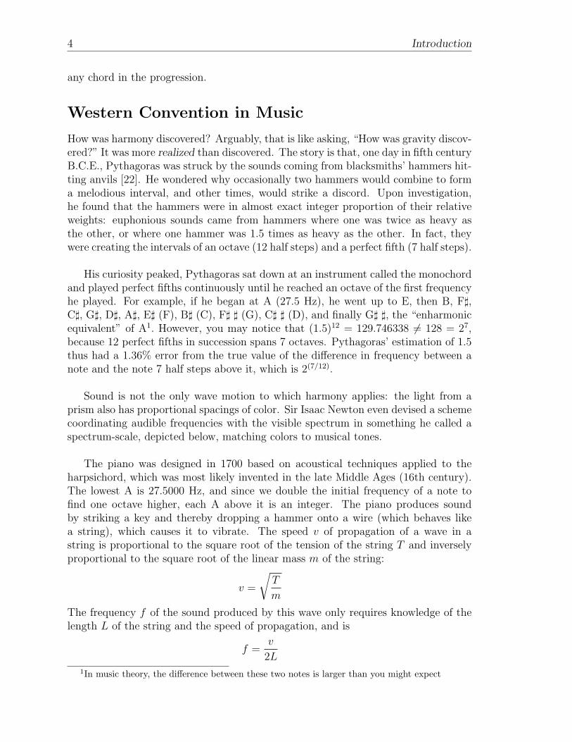
Sound is not the only wave motion to which harmony applies: the light from aprism also has proportional spacings of color. Sir Isaac Newton even devised a schemecoordinating audible frequencies with the visible spectrum in something he called aspectrum-scale, depicted below, matching colors to musical tones.
The piano was designed in 1700 based on acoustical techniques applied to theharpsichord, which was most likely invented in the late Middle Ages (16th century).The lowest A is 27.5000 Hz, and since we double the initial frequency of a note tofind one octave higher, each A above it is an integer. The piano produces soundby striking a key and thereby dropping a hammer onto a wire (which behaves likea string), which causes it to vibrate. The speed v of propagation of a wave in astring is proportional to the square root of the tension of the string T and inverselyproportional to the square root of the linear mass m of the string:
v =
√T
m
The frequency f of the sound produced by this wave only requires knowledge of thelength L of the string and the speed of propagation, and is
f =v
2L1In music theory, the difference between these two notes is larger than you might expect
Introduction 5
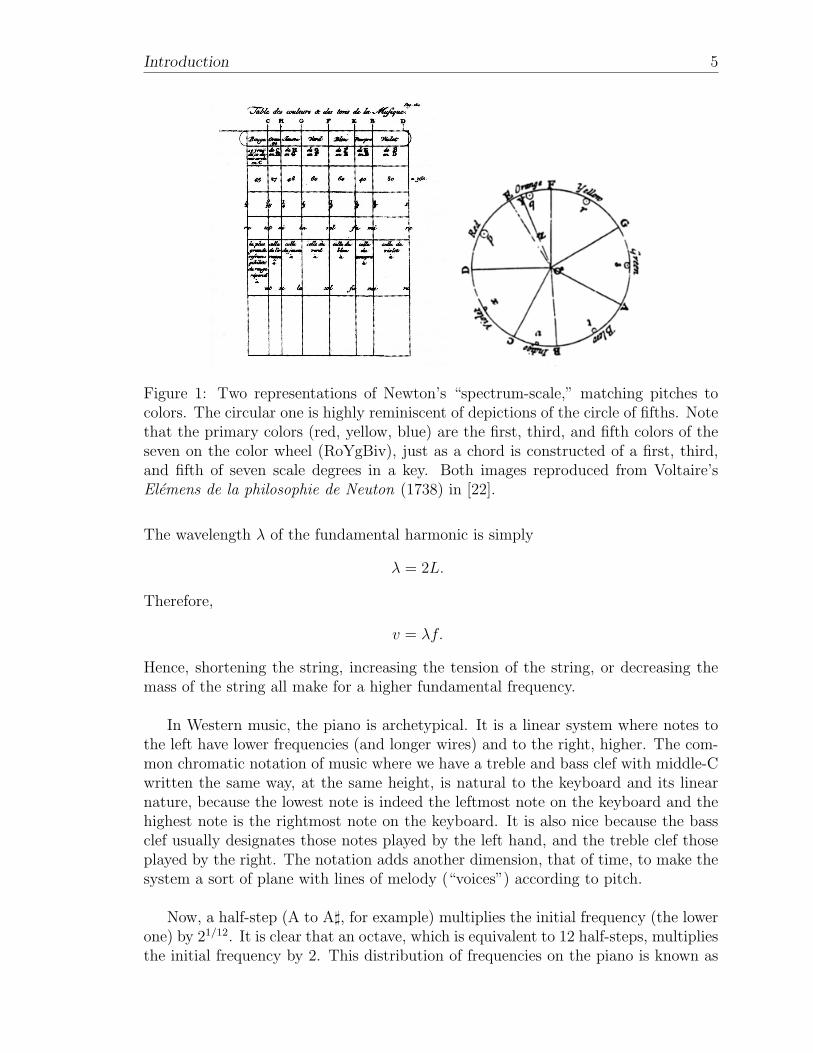
Figure 1: Two representations of Newton’s “spectrum-scale,” matching pitches tocolors. The circular one is highly reminiscent of depictions of the circle of fifths. Notethat the primary colors (red, yellow, blue) are the first, third, and fifth colors of theseven on the color wheel (RoYgBiv), just as a chord is constructed of a first, third,and fifth of seven scale degrees in a key. Both images reproduced from Voltaire’sElemens de la philosophie de Neuton (1738) in [22].
The wavelength λ of the fundamental harmonic is simply
λ = 2L.
Therefore,
v = λf.
Hence, shortening the string, increasing the tension of the string, or decreasing themass of the string all make for a higher fundamental frequency.
In Western music, the piano is archetypical. It is a linear system where notes tothe left have lower frequencies (and longer wires) and to the right, higher. The com-mon chromatic notation of music where we have a treble and bass clef with middle-Cwritten the same way, at the same height, is natural to the keyboard and its linearnature, because the lowest note is indeed the leftmost note on the keyboard and thehighest note is the rightmost note on the keyboard. It is also nice because the bassclef usually designates those notes played by the left hand, and the treble clef thoseplayed by the right. The notation adds another dimension, that of time, to make thesystem a sort of plane with lines of melody (“voices”) according to pitch.
Now, a half-step (A to A], for example) multiplies the initial frequency (the lowerone) by 21/12. It is clear that an octave, which is equivalent to 12 half-steps, multipliesthe initial frequency by 2. This distribution of frequencies on the piano is known as
6 Introduction
“equal temperament,” which has a ring of political incorrectness, since many East-ern cultures use quarter-tones (simply half of a half-step). But we attach a positivemeaning to “harmony,” and indeed the frequencies that occur from a note’s harmonicovertone series are considered “pleasant,” and shape much of Western convention insongwriting.
For more about the notation techniques and harmonic part-writing used in thisthesis, please see Appendix A.
Procedure
This project requires evidence from a vast range of mathematics, acoustics, and musictheory, so I try to develop each relevant discipline as narrowly as possible.
1. We import songs into a series of bandpass filters in parallel, and pick out themost intense frequencies by analyzing their power.
2. We count up the number of times we transition between chord ci and chord cjfor all chords ci and cj s.t. ci 6= cj (or simply, i 6= j) in a progression X withstate space C.
3. We divide these counts by the total number of times we transition from theinitial chord ci and obtain a probability distribution. We insert this as a rowinto a Markovian transition matrix representing a Markov chain, where thechain is a chord progression, in which each row of the matrix sums to 1 and thediagonal entries are 0, since we are not paying mind to rhythm and thereforecannot account for the duration of states.
4. We take the entropy of the Markov chain for each (set of) progression(s) usingthe measure
∑i pi∑
j pj|i logN(1/pj|i), where pi is the probability of hearingchord ci, N is the number of distinct states in C, and pj|i is the probability oftransitioning to chord cj from chord ci.
5. We compare the levels of entropy against each other and see what the measuremeans in terms of the strictness of the musical classification of the set of chords.
The first of these procedures, i.e. filtering and digital signal processing, is de-veloped in the first chapter. The second and third are discussed in Chapter 2 onMarkovian probability. The final two are found in the third chapter on entropy andinformation theory, where the conclusions and some code can be found.2
2Because so many of aspects of this thesis come from very distinct fields of mathematics, physics,and engineering, I would not be surprised to hear that I go into far too much detail trying to describethe elementary nature of each of the fields. However, I wanted to make sure that this document was“compact,” and contained all definitions that one might need to reference. For those that I didn’tstate immediately after their introduction, they can (hopefully) be found in the glossary.
Chapter 1
Automatic Recognition of DigitalAudio Signals
1.1 Digital Audio Signal Processing
Digital signal processing (DSP) originated from Jean Baptiste Joseph, Baron deFourier in his 1822 study of thermal physics, Theorie analytique de la chaleur. There,he “evolved” [10] the Fourier series, applying to periodic signals, and the Fouriertransform, applying to aperiodic, or non-repetitive, signals. The discrete Fouriertransform became popular in the 1940s and 1950s, but was difficult to use withoutthe assistance of a computer because of the huge amount of computations involved.James Cooley and John Tukey published the article “An algorithm for the machinecomputation of complex Fourier series” in 1965, and thereby invented the fast FourierTransform, which reduced the number of computations in the discrete version fromO(n2) to O(n log n) by a recursive algorithm, since roots of unity in the Fourier trans-form behave recursively. Oppenheimer and Schafer’s Digital Signal Processing andRabiner and Gold’s Theory and Application of Digital Signal Processing remain theauthoritative texts on digital signal processing since their publication in 1975, thoughthe highly technical style keeps them fairly inaccessible to the non-electrical engineer.Also, the Hungarian John von Neumann’s architecture of computers from 1946 wasthe standard for more than 40 years because of two main premises: (1) there does notexist an “intrinsic difference” between instructions and data [10], and (2) instructionscan be partitioned into two major fields containing an operation and data upon whichto operate, creating a single memory space for both instructions and data.
Essentially, DSP’s goal is to maximize the signal-to-noise ratio, and it does so withfilters like the discrete Fourier transform, bandpass filters, and many others. Digitalmedia is always discrete, unlike its analog predecessor, but the digital form has itsadvantages. For one, a CD or vinyl will deteriorate over time, or become soiled andscratched, and this does not happen to digital files. Second, it is easy and fast toreplicate a digital version and store it in many places, again increasing the likelihoodof maintaining its original form. Finally, with analog’s “infinite sampling rate” [10]comes infinite variability, and this also contributes to digital media’s robustness over
8 Chapter 1. Automatic Recognition of Digital Audio Signals
analog.To sample a signal, we take a discrete impulse function, element-wise multiply it
(i.e., take the dyadic product of it) with an analog signal, and retrieve a sampling ofthat signal with which we can do many things. The construction of a filter essentiallylies in the choice of coefficients; we will go through a proof of our choice in coefficientsto show that the filtering works.
1.1.1 Sampling
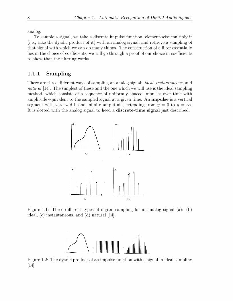
There are three different ways of sampling an analog signal: ideal, instantaneous, andnatural [14]. The simplest of these and the one which we will use is the ideal samplingmethod, which consists of a sequence of uniformly spaced impulses over time withamplitude equivalent to the sampled signal at a given time. An impulse is a verticalsegment with zero width and infinite amplitude, extending from y = 0 to y = ∞.It is dotted with the analog signal to heed a discrete-time signal just described.
Figure 1.1: Three different types of digital sampling for an analog signal (a): (b)ideal, (c) instantaneous, and (d) natural [14].
Figure 1.2: The dyadic product of an impulse function with a signal in ideal sampling[14].
1.1. Digital Audio Signal Processing 9
Formally, this is given by
xs(t) = x(t) · (δ(t−∞) + . . .+ δ(t− T ) + δ(t) + δ(t+ T ) + . . .+ δ(t+∞))
= x(t)∞∑
n=−∞
δ(t− nT )
where xs(t) is the sampled (discrete-time) signal, δ is the impulse function, and T isthe period of x(t), i.e., the spacing between impulses. We compute the power p at apoint in time t
p(t) = |x(t)|2
and the energy of a system, or entire signal
E =∞∑
t=−∞
|x(t)|2.
Energy is measured in joules, where 1 joule is 1 watt × 1 second. The average powerP is then
P = limT→∞
1
2T
T∑t=−T
|x(t)|2.
A signal has a minimum frequency fL (it is fine to assume that this is 0 Hz, inmost applications) and a maximum frequency fU . If a signal is undersampled, i.e.,the sampling frequency is fs < 2 · fU , the impulses will not be spaced far enoughapart, and the resulting spectrum will have overlaps. This is known as aliasing, andwhen two spectra overlap, they are said to alias with each other. We have a theoremthat forebodes the problems that occur from undersampling.
The Nyquist-Shannon Sampling Theorem. If a signal x(t) contains no fre-quencies greater than fU cycles per second (Hz), then it is completely determined bya series of points spaced no more than 1
2fUseconds apart, i.e., the sampling frequency
fs ≥ 2fU . We reconstruct x(t) with the function
x(t) =∞∑
n=−∞
x(nT )sin[2fs(t− nT )]
2fs(t− nT ).
The minimum sampling frequency is often referred to as the Nyquist frequencyor Nyquist limit, and this rate of 1
2fUis referred to as the Nyquist rate. The
bandwidth of a signal is its highest frequency component, fU .
Aliasing is depicted in the following sequence of images, all taken from [7]. Theconstruction of the impulse function is crucial to avoiding aliasing.
10 Chapter 1. Automatic Recognition of Digital Audio Signals
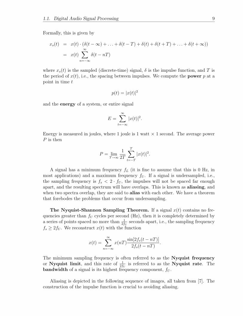
Figure 1.3: The impulse function δ for sampling a signal at ωs.
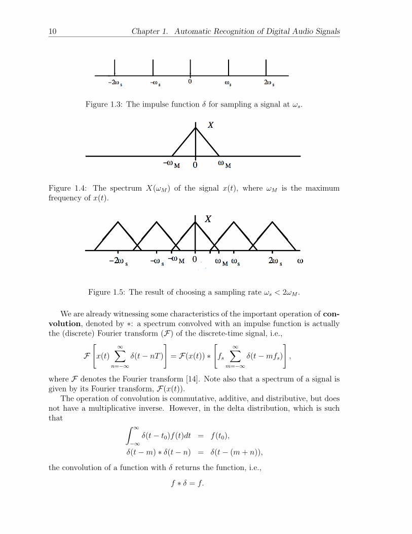
Figure 1.4: The spectrum X(ωM) of the signal x(t), where ωM is the maximumfrequency of x(t).
Figure 1.5: The result of choosing a sampling rate ωs < 2ωM .
We are already witnessing some characteristics of the important operation of con-volution, denoted by ∗: a spectrum convolved with an impulse function is actuallythe (discrete) Fourier transform (F) of the discrete-time signal, i.e.,
F
[x(t)
∞∑n=−∞
δ(t− nT )
]= F(x(t)) ∗
[fs
∞∑m=−∞
δ(t−mfs)
],
where F denotes the Fourier transform [14]. Note also that a spectrum of a signal isgiven by its Fourier transform, F(x(t)).
The operation of convolution is commutative, additive, and distributive, but doesnot have a multiplicative inverse. However, in the delta distribution, which is suchthat ∫ ∞
−∞δ(t− t0)f(t)dt = f(t0),
δ(t−m) ∗ δ(t− n) = δ(t− (m+ n)),
the convolution of a function with δ returns the function, i.e.,
f ∗ δ = f.
1.1. Digital Audio Signal Processing 11
1.1.2 The Discrete Fourier Transform
The Discrete Fourier Transform (DFT) and its inverse (the IDFT) are used on ape-riodic signals to establish which peak frequencies are periodic (i.e., are overtones1),and those that are aperiodic. The DFT represents the spectrum of a signal, and theIDFT reconstructs the signal (with a phase shift) and retrieves only those frequenciesthat are fundamental. It is a heavy but simple algorithm with many variables, so it isbest to approach it slowly to truly understand its mechanisms2. It was born from theFourier series in Fourier analysis, and it attempts to approximate the abstruse wavesof a spectrogram by simpler trigonometric piecewise functions, for the behavior of afrequency can be modeled by sinusoidal functions. This helps clarify what is noisein a signal and what is information by reducing a signal to a sufficiently large, finitenumber of its fundamental frequencies in a given finite segment of the signal.
Definition: Fourier transform. The Fourier transform is an invertible lineartransformation
F : CN → CN
where C denotes the complex numbers. Hence, it is complete. The Fourier transformof a continuous-time signal x(t) is represented by the integral [34]
X(ω) =
∫ ∞−∞
x(t)e−iωtdt, and inversely,
x(t) =
∫ ∞−∞
X(ω)eiωtdω, ω ∈ R,
where X(ω) is the spectrum of x at frequency ω.
It is not difficult to see why the discrete-time signal case is then represented by
X(ωk) =N−1∑n=0
x(tn)e−iωktn , k = 0, 1, 2, . . . , N − 1,
which, because ωk = 2πk/(NT ) and tn = nT , can also be written
X(k) =N−1∑n=0
x(n)e−i2πkn/N , k = 0, 1, 2, . . . , N − 1,
and the inverse DFT, or IDFT, is
x(tn) =1
N
N−1∑k=0
X(ωk)eiωktn , n = 0, 1, 2, . . . , N − 1,
1The overtone series of a fundamental frequency is the sequence of frequencies resulting frommultiplying the fundamental frequency by each of the natural numbers (i.e., 1 ·ffund, 2 ·ffund, . . .).The overtone series of A=55 Hz is 55 Hz = A, 110 Hz = A, 165 Hz = E, 220 Hz=A, 275 Hz=C ],330 Hz = E, 385 Hz=G, 440 Hz=A, 495 Hz=B [, . . ..
2The book [34] is a very good resource for those new to the Fourier transform.
12 Chapter 1. Automatic Recognition of Digital Audio Signals
which similarly can be rewritten
x(n) =1
N
N−1∑k=0
X(k)ei2πkn/N , n = 0, 1, 2, . . . , N − 1.
List of symbols in the DFT.
:= := “defined as”
x(t) := the amplitude (real or complex) of the input signal at time t (seconds)
T := the sampling interval, or period, of x(t)
t := t · T = sampling instant, t ∈ NX(ωk) := spectrum of x at frequency ωk
ωk := kΩ = kthfrequency sample
Ω :=2π
NT= radian-frequency sampling interval (radians/sec)
ω := 2πfs
fs := 1/T =ω
2π= the sampling rate, in hertz (Hz)
N := the number of time samples = the number of frequency samples ∈ Z+
The signal x(t) is called a time domain function and the corresponding spectrumX(k) is called the signal’s frequency domain representation. The amplitude A ofthe DFT X is given by
A(k) = |X(k)| =√<(X(k))2 + =(X(k))2,
and its phase φ is
φ(k) = 2 arctan=(X(k))
|X(k)|+ <(X(k))
This trigonometric function finds the angle in radians between the positive x-axisand the coordinate (=(X(k)),<(X(k))). It is positive and increasing from (0, π)(counter-clockwise), and negative and decreasing from (0,-π) (clockwise). It equals πat π.
You may notice that the exponentials in both the DFT and its inverse resembleroots of unity, of which Euler’s identity will be helpful in explaining.
Euler’s identity. For any real number x,
eix = cos x+ i sinx, and
e−ix = cos x− i sinx.
Definition: Roots of unity. We call the set W = W 0N ,W
1N , . . . ,W
N−1N the
N th roots of unity corresponding to points on the unit circle in the complex plane,
1.1. Digital Audio Signal Processing 13
where
WN = e2πiN , the primitive N th root of unity;
W kN = e
2πikN = (WN)k, the kth N th root of unity;
WNN = W 0
N .
By Euler’s identity,
W knN = e
2πiknN = cos(2πkn/N) + i sin(2πkn/N).
This is called the “kth sinusoidal function of f” [34].By Euler’s identity, e−i2πkt/N = cos(2πkt/N) − i sin(2πkt/N) and ei2πkt/N =
cos(2πkt/N) + i sin(2πkt/N). Therefore, we can also write the DFT and its inverseas follows:
X(k) =N−1∑t=0
x(t)e−i2πkt/N , k = 0, 1, . . . , N − 1
=N−1∑t=0
x(t) cos(2πkt/N)− iN−1∑t=0
x(t) sin(2πkt/N)
x(t) =1
N
N−1∑k=0
X(k)ei2πkt/N , t = 0, 1, . . . , N − 1
=1
N
N−1∑k=0
X(k) cos(2πkt/N) +i
N
N−1∑k=0
X(k) sin(2πkt/N).
Then,
e−i2πkt/N = cos(2πkt/N)− i sin(2πkt/N)
is the kernel of the discrete Fourier transform.For the sake of clarity, I will show that the IDFT is indeed the inverse of the DFT.
To do so, all we need to note is the boundedness of k in either of the sums:
X(k) =N−1∑t=0
x(t)e−2πitkN
=N−1∑t=0
(1
N
N−1∑k=0
X(k)e2πitkN
)e−2πitkN
Since the k in e−2πitkN is not bounded by the k in the inner sum, we change the inside
14 Chapter 1. Automatic Recognition of Digital Audio Signals
k to l:
=N−1∑t=0
(1
N
N−1∑l=0
X(l)e2πitlN e
−2πitkN
)
=N−1∑t=0
1
N
N−1∑l=0
X(l)e2πit(l−k)
N
=1
N
N−1∑l=0
X(l)N−1∑t=0
e2πit(l−k)
N
= N when l = k, 0 otherwise
Thus, our double sum is
1
N
N−1∑l=0
X(l)Nδlk = X(k),
where δlk = 1 for l = k and 0 otherwise.
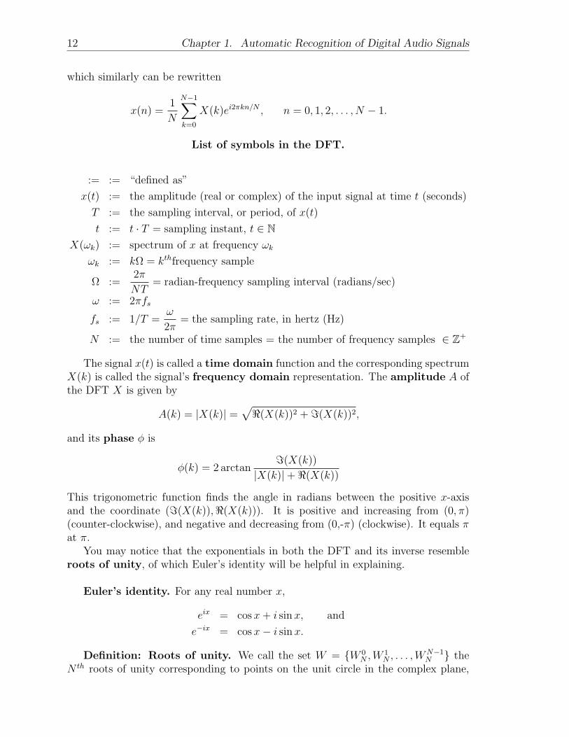
To help you visualize how the DFT and IDFT manipulate a signal, four examplesof signals are shown in Figures 1.6-1.9: two are periodic, two aperiodic, two noiseless,and two containing noise. All transforms are absolute values; note the phase shift inthe IDFT reconstruction when the signal contains negative values.
Figure 1.6: Noiseless periodic signal, its DFT, and its IDFT.
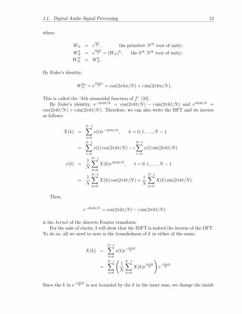
Figure 1.7: Noisy periodic signal, its DFT, and its IDFT.
Note that the transforms are symmetric about the middle term, k = t = N/2, theNyquist frequency. This happens because the signals are real-valued. For complex-valued signals, the Nyquist frequency is always zero.
1.1. Digital Audio Signal Processing 15
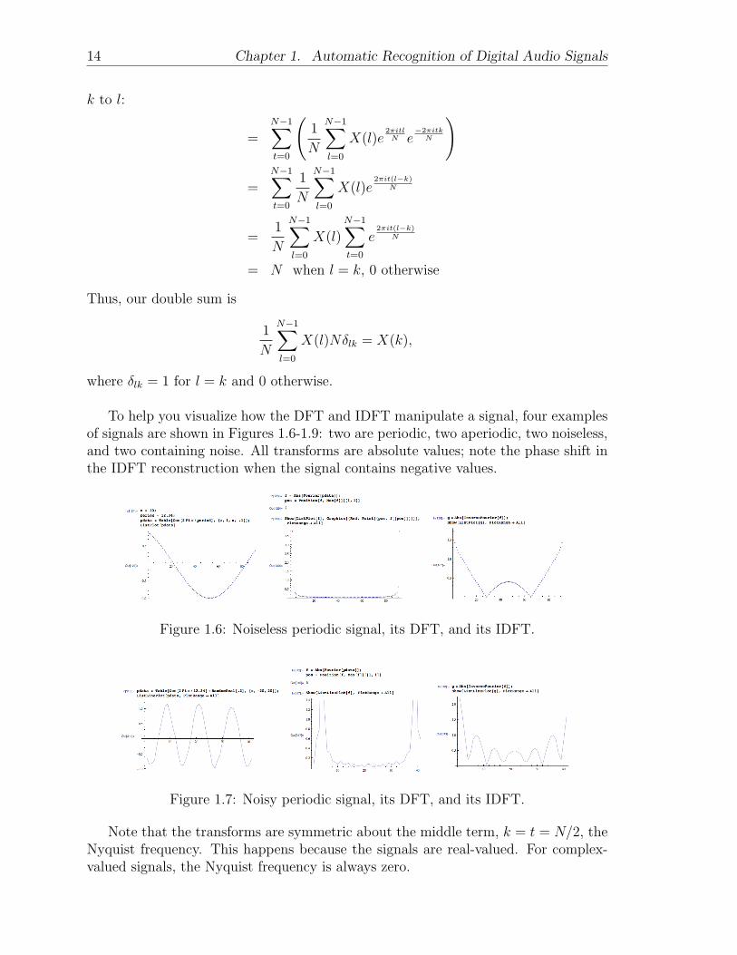
Figure 1.8: Noiseless aperiodic signal, its DFT, and its IDFT.
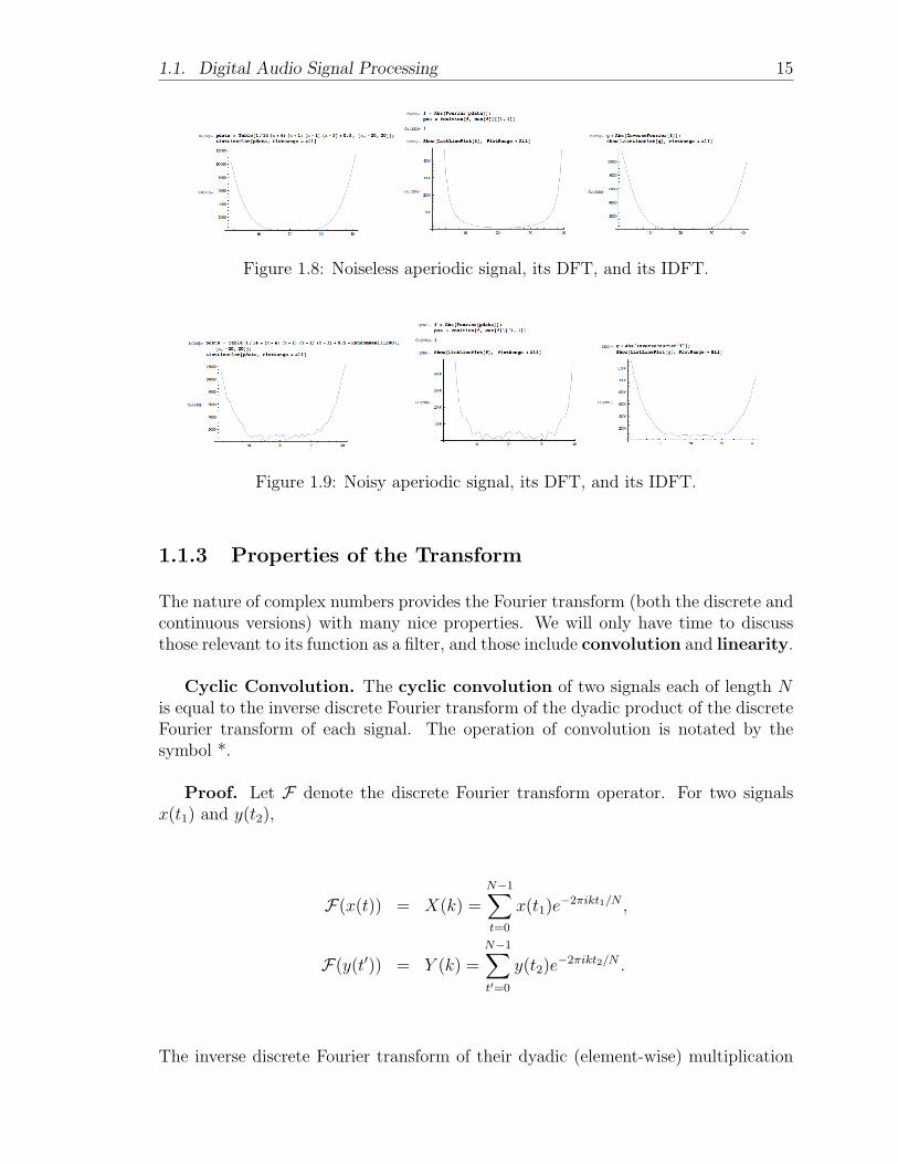
Figure 1.9: Noisy aperiodic signal, its DFT, and its IDFT.
1.1.3 Properties of the Transform
The nature of complex numbers provides the Fourier transform (both the discrete andcontinuous versions) with many nice properties. We will only have time to discussthose relevant to its function as a filter, and those include convolution and linearity.
Cyclic Convolution. The cyclic convolution of two signals each of length Nis equal to the inverse discrete Fourier transform of the dyadic product of the discreteFourier transform of each signal. The operation of convolution is notated by thesymbol *.
Proof. Let F denote the discrete Fourier transform operator. For two signalsx(t1) and y(t2),
F(x(t)) = X(k) =N−1∑t=0
x(t1)e−2πikt1/N ,
F(y(t′)) = Y (k) =N−1∑t′=0
y(t2)e−2πikt2/N .
The inverse discrete Fourier transform of their dyadic (element-wise) multiplication
16 Chapter 1. Automatic Recognition of Digital Audio Signals
is
F−1(F(x(t1)) · F(y(t2))) =1
N
N−1∑k=0
X(k)Y (k)e2πitk/N
=1
N
N−1∑k=0
(N−1∑t1=0
x(t1)e−2πikt1/N
)(N−1∑t2=0
y(t2)e−2πikt2/N
)ei2πkt/N
=1
N
N−1∑t1=0
N−1∑t2=0
x(t1)y(t2)N−1∑k=0
e2πik(t−(t1+t2))/N .
Summing over k, we get
N−1∑k=0
e2πik(t−(t1+t2))/N = Nδ,
where δ is 1 when n ≡ (t1 + t2) mod N and 0 otherwise. Therefore, the above triplesum becomes ∑
t1+t2≡t mod N
x(t1)y(t2) =N−1∑t1=0
x(t1)y(t− t1)
=N−1∑t2=0
x(t− t2)y(t2)
= x ∗ y(t),
which proves the theorem.
Corollary.
F(x(t) · y(t)) = F(x(t)) ∗ F(y(t)).
This is how we obtain the aforementioned result
F
[x(t)
∞∑n=−∞
δ(t− nT )
]= F(x(t)) ∗
[fs
∞∑m=−∞
δ(t−mfs)
].
Another important property of the Fourier transform is its linearity.
Linearity of the DFT. A signal x can be scaled by a constant a such thatF(a · x) = a ·X.
Proof.
ax(t) =a
N
N−1∑t=0
X(f)ei2πft/N
= aX(f).
1.1. Digital Audio Signal Processing 17
Also, the sum of two signals equals the sum of their transforms, i.e., a · x+ b · y =a ·X + b · Y , a and b constants.
Proof.
ax(t) + by(t) =a
N
N−1∑t=0
X(f)ei2πft/N +b
N
N−1∑t=0
Y (f)ei2πft/N
= aX(f) + bY (f).
The DFT is called a linear filter because of these properties, and it is time-invariant or time-homogeneous, meaning that over time, it does not change.
One final interesting property of the DFT that is likely relevant to filtering, thoughI have not come across a literal relevance, is in Parseval’s theorem, which statesthat
N−1∑t=0
|x(t)|2 =1
N
N−1∑k=0
|X(k)|2,
or, the DFT is unitary. A more general form of Parseval’s theorem is Plancherel’stheorem [33].
The Fourier transform can be used to detect instrumentation, because each in-strument (including each person’s voice) has a unique timbre. Timbre means “tonecolor,” and is simply the word we use to distinguish a note played by a violin fromthe same note played by a piano. Timbre affects the amplitudes of a frequency’sovertone series, which is the sequence of frequencies found by multiplying the fun-damental frequency by each of the natural numbers (i.e., 1 ·ffund, 2 ·ffund, . . .). So,in this way, the human ear is foremost a Fourier device: it can distinguish betweeninstruments, just as it can other humans’ voices. However, computers give us thedetails about what it is that makes the quality of voices differentiable. Although thisis fascinating, we will not be paying mind to timbre in this project, which I am surewill prove problematic in trying to separate the (background) chord progression fromthe (foreground) melody.
1.1.4 Filtering
We use a filter when we want to retrieve a single frequency or set of frequenciesfrom a signal, and decimate the remainder. Decimation via digital filtering is calledattenuation. One way to think of a digital filter is as a Kronecker delta function.It is a spectrum with amplitude 1 at the frequencies it is designed to maintain ina signal, and amplitude 0 at the frequencies it is designed to kill. But because itis a continuous function, it contains amplitudes in between 0 and 1, and where theamplitude is 0.5 is called a cutoff frequency. There can be only zero, one, or twocutoff frequencies in the filters described below.
18 Chapter 1. Automatic Recognition of Digital Audio Signals
In working with digital signals, we use Finite Impulse Response (FIR) techniques[14]. An important concept in digital filtering is the impulse response h(t), whichis a measure of how the outputted signal responds to a unit impulse from the im-pulse function δ. A unit impulse is given by δ(t), the continuous case of familiarKronecker delta function. Both a filter and a signal have an impulse function. Wecan integrate or sum over the impulse response to obtain the step response a(t), anduse the Laplace transform, a definition of which can be found in the glossary butis beyond the scope of this thesis, to obtain the transfer function H(s), wheres = 1−z
1+z, z from the z-transform, also beyond the scope of this thesis but defined in
the glossary.The general form for a linear time-invariant FIR system’s output y at time t is
given by
y(t) =N−1∑τ=0
h(τ)x(t− τ)
=N−1∑T=0
h(t− T )x(T )
by a change of variables, T = t− τ .Filters are specified by their frequency response H(f), which is the discrete
Fourier transform of the impulse response h(t).
H(f) =N−1∑t=0
h(t)e−i2πtf/N , f = 0, 1, . . . , N − 1.
A filter modifies the frequencies within the spectrum (DFT) of a signal. When wewant to rid a signal of frequencies below some cutoff (or critical) frequency fc, suchthat we are left with only frequencies above fc, we design a highpass filter. Itsimpulse response is defined for a user-defined value N equal to the number of taps,or the number of frequencies, at which the response is to be evaluated, and is givenby
h(t) = h(N − 1− t) = −sin(mλc)
mπ
where m = t− N−12
and λc = ωcT = 2πfcT . If N is odd, then we compute
h
(N − 1
2
)= 1− λc
π.
Like the discrete Fourier transform and its inverse, the impulse response is symmetricabout t = N
2for N even or about t = N−1
2for N odd, and therefore half-redundant.
But since audio signals are real-valued, the Nyquist frequency is not necessarily 0.Now, for a lowpass filter in which only low frequencies, or those below some fc,
may “pass through,” our impulse response function is
h(t) = h(N − 1− t) =sin(mλc)
mπ,
1.2. A Tunable Bandpass Filter in Mathematica 19
where again m = t− N−12
and λc = 2πfcT . If N is odd, then
h
(N − 1
2
)=λcπ.
Putting the two together is one way of designing a bandpass filter, whose pass-band (the resulting bandwidth of any kind of “pass” filter) is restricted by a lowercritical frequency, fl, and an upper critical frequency, fu. If fl = fL, the minimumfrequency in the signal, and fu = fU , the maximum frequency in the signal, then thefilter is an all pass filter. Its impulse response function is
h(t) = h(N − 1− t) =1
mπ[sin(mλu)− sin(mλl)]
and once again m = t− N−12
and λu = 2πfuT, λl = 2πflT . If N is odd, then we have
h
(N − 1
2
)=λu − λlπ
.
The opposite of a bandpass filter is a bandstop filter or notch filter. Its impulseresponse is given by
h(t) = h(N − 1− t) =1
tπ[sin(mλl)− sin(mλu)].
For odd N ,
h
(N − 1
2
)= 1 +
λl − λuπ
.
Again, m, λl, and λu are all defined as above.All of these impulse response functions output the coefficients for an N -tap filter
of their type, and the IDFT gives the corresponding discrete-time impulse response[14].
1.2 A Tunable Bandpass Filter in Mathematica
1.2.1 Design
A bandpass filter takes an input of a frequency f , quality Q, and signal x, andoutputs a signal with bandwidth centered at f . It does not matter whether f existsin the spectrum, but if it does, the bandpass filter gets excited, and shows that thefrequency contributes to the amplitude (power) of the signal. The value Q is positiveand real, and a high Q (¿20) means a sharp focus around this “resonant” frequency fby defining the sinusoid to have a dramatic and steep peak centered at f , where a lowQ means a gentler-sloped sinusoid is chosen for the filter. In essence, Q determineshow quickly the impulse response of a filter goes from 0 to 1, and/or 1 to 0.
20 Chapter 1. Automatic Recognition of Digital Audio Signals
When dealing with a digital signal, we must tune our desired frequency to takethe sampling frequency into account. We do this by scaling f by 2π
fs, where fs is the
sampling frequency. We name the tuned frequency θf = 2πfs· f .
To show that the coefficients
β =1
2
1− tan(θf2Q
)1 + tan
(θf2Q
) ,
α =1
2
(1
2− β
),
γ =
(1
2+ β
)cos(θf )
in the recursion
y(t) = 2 (α (x(t)− x(t− 2)) + γy(t− 1)− βy(t− 2))
will define such a filter, let us prove them using the Ansatz (“onset”) solution method,where we will let A(θf ) designate our educated guess.
Proof. Since we know that x(t) and likewise its filtered signal y(t) are sinusoidalfunctions, let
x(t) = eiωt,
y(t) = A(ω)x(t).
Then we can solve for A by
A(ω)eiωt = 2(α(eiωt − eiω(t−2)
)+ γ
(A(ω)eiω(t−1)
)− β
(A(ω)eiω(t−2)
))A(ω)
2= α(1− e−2iω) + γA(ω)e−iω − βA(ω)e−2iω
= α− αe−2iω + γA(ω)e−iω − βA(ω)e−2iω.
Therefore,
A(ω) ·(
1
2− γe−iω + βe−2iω
)= α− αe−2iω
making A the ratio
A(ω) =α− αe−2iω
12− γe−iω + βe−2iω
.
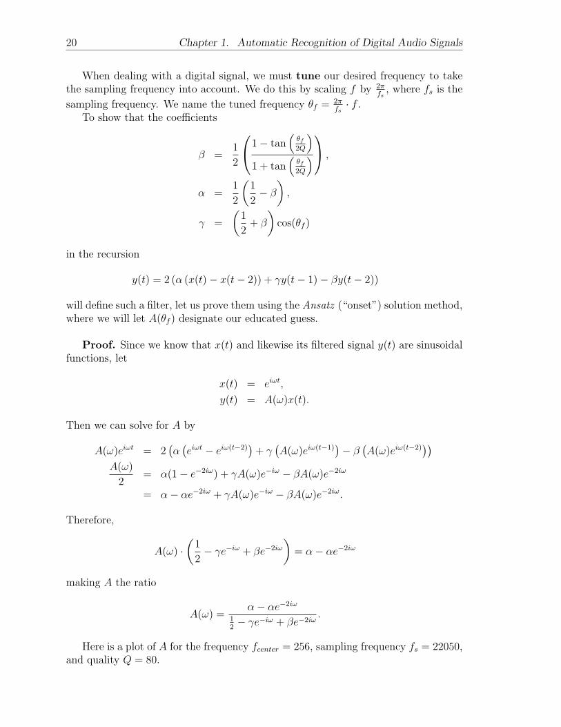
Here is a plot of A for the frequency fcenter = 256, sampling frequency fs = 22050,and quality Q = 80.
1.2. A Tunable Bandpass Filter in Mathematica 21
We will show that A is indeed our ideal curve for bandpass filtering.We can define Q precisely by the ratio [13]
Q =fcenterfu − fl
,
where fu is the high cutoff frequency and fl is the low cutoff frequency of the filter.The frequencies fl and fu are cutoff frequencies because they determine the domain forwhich the amplitude of the filter |A| ≥ 0.5, meaning frequencies outside this domainare attenuated, or decimated, and those inside the domain appear in the passband.The difference fu − fl is the bandwidth of the passband.
Since θf is simply the frequency f scaled, Q is also the ratio
Q =θfcenterθfu − θfl
.
So, for our parameters for Q and fcenter, it should be the case in A that fu− fl =fcenter/Q = 256/80 = 3.2 Hz, the bandwidth of the filter, and judging by the apparentsymmetry of A, the cutoff frequencies should be close to fu = 256 + 1.6 = 257.6 Hzand fl = 256−1.6 = 254.4 Hz. When we tune the filter, the width of A at half-power(A = 0.5± 0.5i, or |A| = 0.5) is the ratio
θ256Hz
Q=
2 · π · 256
22050 · 80= 0.0009118455.
Now, |A(θf )| = 0.5 at θfl = 0.0724931385 and θfu = 0.073404984, meaning that theuntuned cutoff frequencies are fl = 254.404991 Hz and fu = 257.604991 Hz. Theirdifference is θfu− θfl = 0.0009118455, exactly the expected width of A for the quality
22 Chapter 1. Automatic Recognition of Digital Audio Signals
Q = 80, and the ratios
maxθf (A(θf ))
θfu − θfl=
θ256 Hz
θ257.604991 Hz − θ254.404991 Hz
=0.07294763904 Hz
0.0009118455 Hz= 80
= Q
and
fcenterfu − fl
=256 Hz
257.604991 Hz− 254.404991 Hz
=256 Hz
3.2 Hz= 80
= Q
are as expected.
1.2.2 Implementation
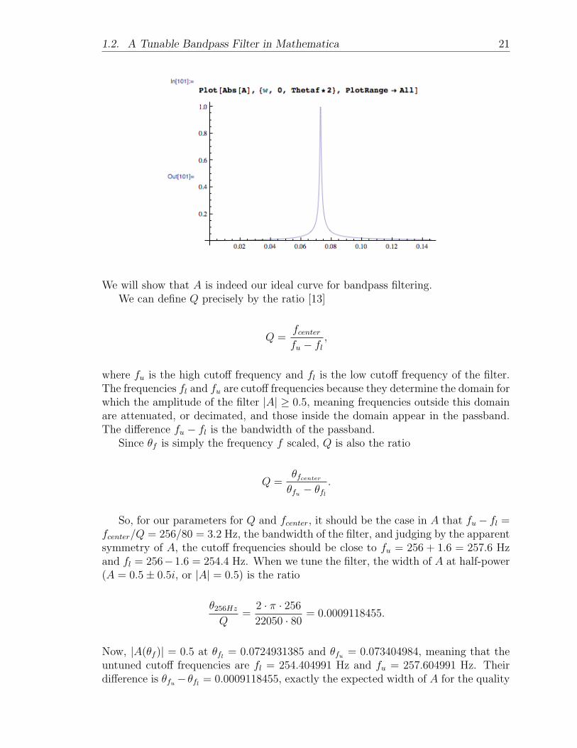
To demonstrate how our bandpass filter picks out a given frequency, we will designa 13 note scale, C to C, in Mathematica. Since we do not change Q for differentfrequencies, this filter is called a constant-Q bandpass filter.
The “SampleRate” set to 22050 indicates that the frequency resolution of ourfilter is 22050 Hz, or 22050 samples per second. CD-quality sound has a frequencyresolution of 44100 Hz, so when it sampled at only 22050 Hz, the sound has twicethe duration. The “SampleDepth” indicates the amplitude resolution of our filter.At 16, each sample therefore may have any of 216 = 65536 amplitudes [13]. Now, thefilter itself contains an initial frequency f ; a “tuning” θf (designated below by T0)equal to 2πf divided by the frequency resolution; and the quality Q, hard-wired at80. The 3 coefficients, α, β, and γ, are constructed from θf and Q (as shown in the
1.2. A Tunable Bandpass Filter in Mathematica 23
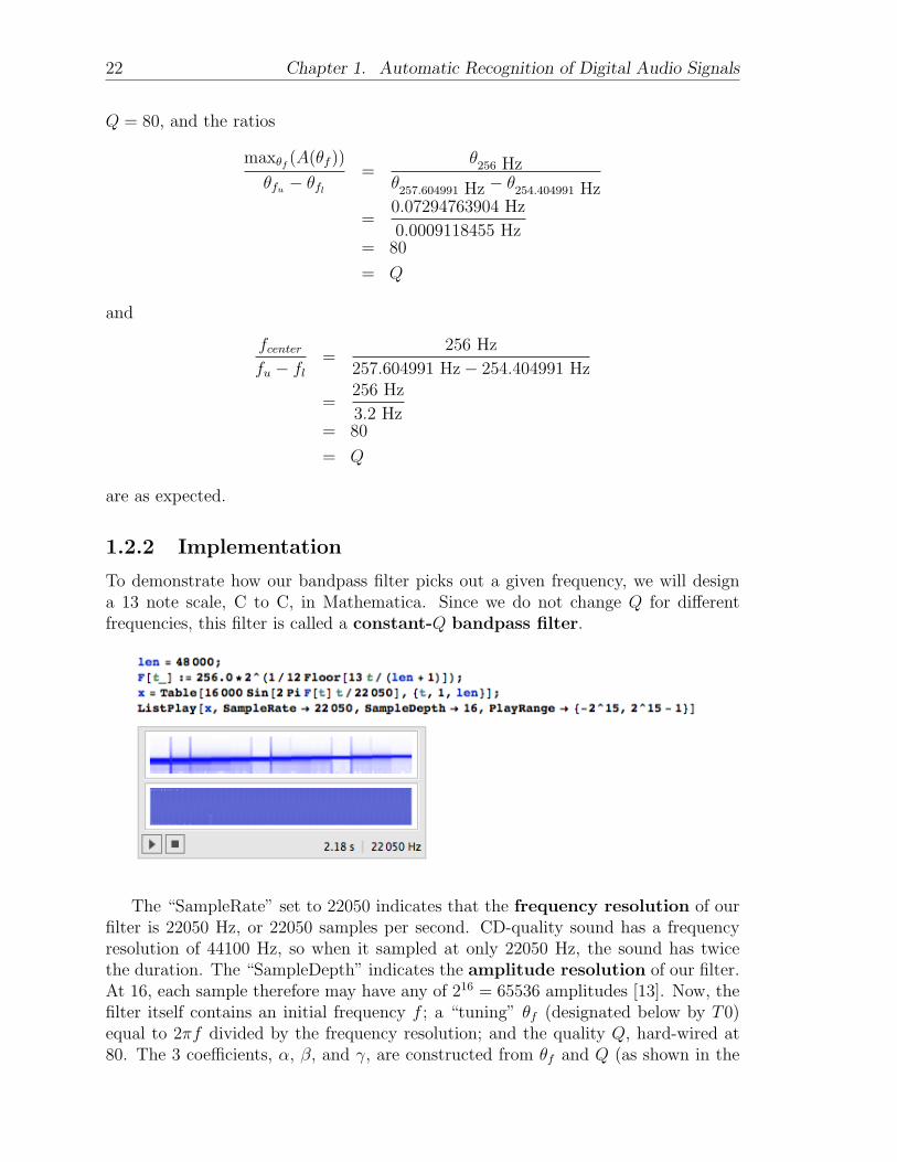
proof by Ansatz above) to change our signal x into a filtered signal y:
We calculate the total power, or energy, of the sound through the bandpass filterin the function BandPower(x, f,Q) by, as defined above, squaring the terms and thensumming them. Since we chose 440 Hz (A) to be our initial frequency (it is the onlypiano frequency that is an integer, not to mention the most common reference pointamongst musicians since it lies within our vocal range and is close in proximity tothe center of the keyboard, middle-C), 9 steps down will give us middle-C, at 261.626Hz.
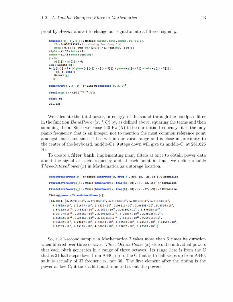
To create a filter bank, implementing many filters at once to obtain power dataabout the signal at each frequency and at each point in time, we define a tableThreeOctavePower(x) in Mathematica as a storage location.
So, a 2.1-second sample in Mathematica 7 takes more than 6 times its durationwhen filtered over three octaves. ThreeOctavePower(x) stores the individual powersthat each pitch generates in a range of three octaves. Its range here is from the Cthat is 21 half steps down from A440, up to the C that is 15 half steps up from A440,so it is actually of 37 frequencies, not 36. The first element after the timing is thepower at low C; it took additional time to list out the powers..
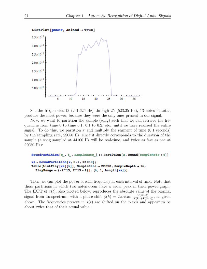
24 Chapter 1. Automatic Recognition of Digital Audio Signals
So, the frequencies 13 (261.626 Hz) through 25 (523.25 Hz), 13 notes in total,produce the most power, because they were the only ones present in our signal.
Now, we want to partition the sample (song) such that we can retrieve the fre-quencies from time 0 to time 0.1, 0.1 to 0.2, etc. until we have realized the entiresignal. To do this, we partition x and multiply the segment of time (0.1 seconds)by the sampling rate, 22050 Hz, since it directly corresponds to the duration of thesample (a song sampled at 44100 Hz will be real-time, and twice as fast as one at22050 Hz):
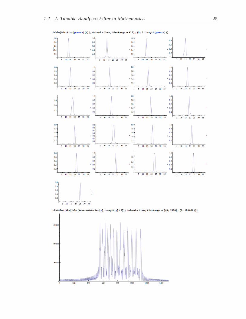
Then, we can plot the power of each frequency at each interval of time. Note thatthose partitions in which two notes occur have a wider peak in their power graph.The IDFT of x(t), also plotted below, reproduces the absolute value of the original
signal from its spectrum, with a phase shift φ(k) = 2 arctan =(X(k))|X(k)|+<(X(k))
, as given
above. The frequencies present in x(t) are shifted on the x-axis and appear to beabout twice that of their actual value.
1.2. A Tunable Bandpass Filter in Mathematica 25
26 Chapter 1. Automatic Recognition of Digital Audio Signals
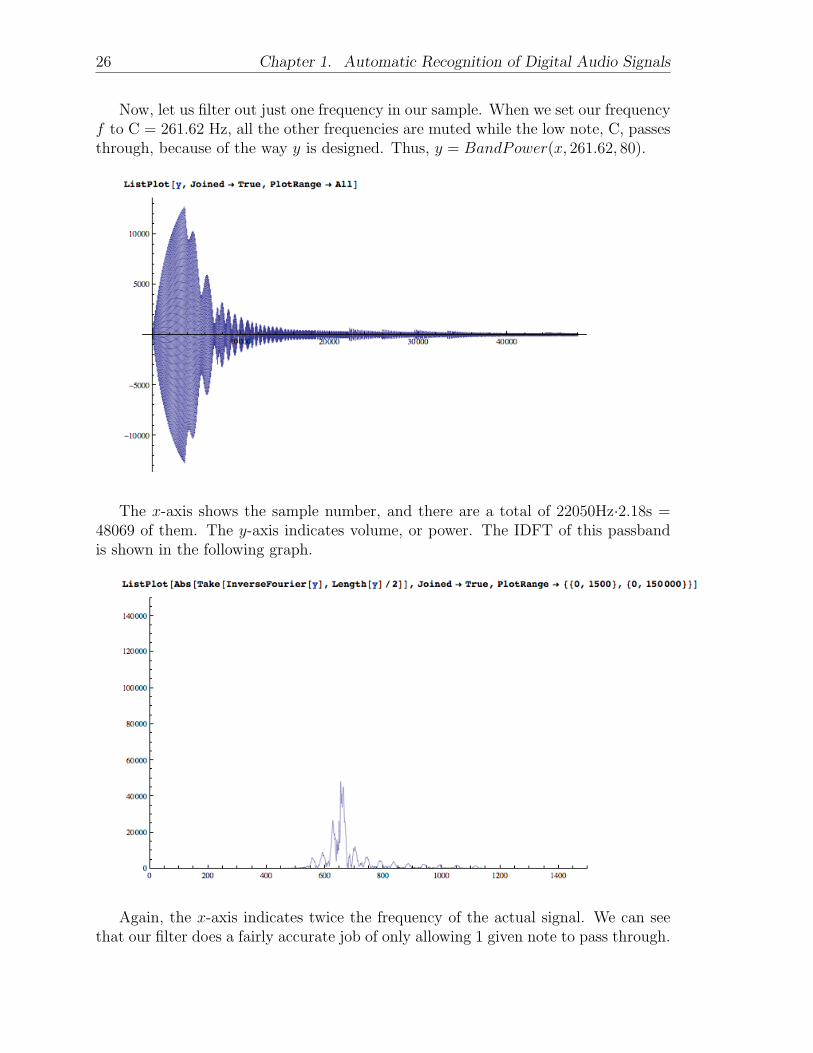
Now, let us filter out just one frequency in our sample. When we set our frequencyf to C = 261.62 Hz, all the other frequencies are muted while the low note, C, passesthrough, because of the way y is designed. Thus, y = BandPower(x, 261.62, 80).
The x-axis shows the sample number, and there are a total of 22050Hz·2.18s =48069 of them. The y-axis indicates volume, or power. The IDFT of this passbandis shown in the following graph.
Again, the x-axis indicates twice the frequency of the actual signal. We can seethat our filter does a fairly accurate job of only allowing 1 given note to pass through.
1.2. A Tunable Bandpass Filter in Mathematica 27
If we increased Q, we might get even more precise results, but Q = 80 seems to besufficient for this project.
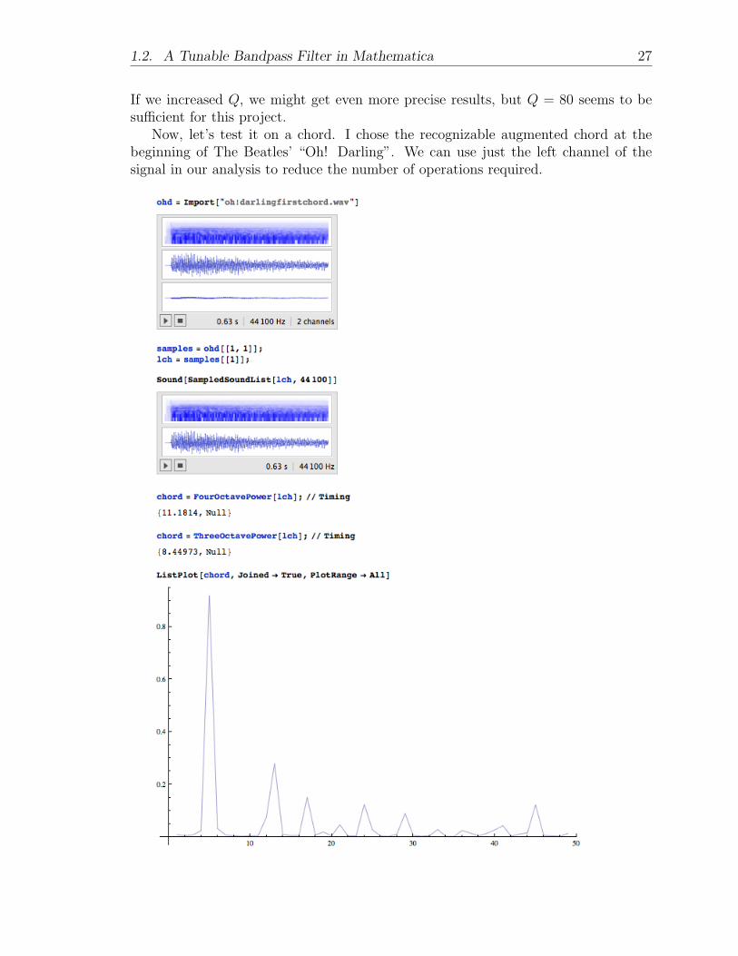
Now, let’s test it on a chord. I chose the recognizable augmented chord at thebeginning of The Beatles’ “Oh! Darling”. We can use just the left channel of thesignal in our analysis to reduce the number of operations required.
28 Chapter 1. Automatic Recognition of Digital Audio Signals
The 0.63 second sample through 49 bandpass filters for four octaves (plus highC) takes 1.323 times the time the three octave (37 filters) module takes, which isapproximately the ratio 49/37 = 1.324. Thus, we can expect this program to run inapproximately 13.412 times the length of the sample.
Finally, we retrieve the normalized powers of each note in the three octave spec-trum, and see peaks at 5, 13, 17, 24, 29, and 45. We add 47 to each of these to getthe MIDI keyboard equivalent, playable through GarageBand and similar platforms,and got E=52, B=59, C=60, E=64, B=71, E=76, and G]=92, which actually spellout an augmented C-seventh chord, but the peak at E makes it clear that it is theroot and that the B is incorrect. Indeed, it is an overtone of E, and the actual chordplayed is an E+ (augmented) chord.
1.3 A Tunable Bandpass Filter in C
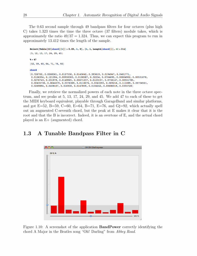
Figure 1.10: A screenshot of the application BandPower correctly identifying thechord A Major in the Beatles song “Oh! Darling” from Abbey Road.
1.3. A Tunable Bandpass Filter in C 29
To run a 3-minute song in Mathematica would take some 40 minutes, a grossamount of memory, and all of my very current MacBook Pro’s 2.4 GHz dual processorpower, so naturally, the main thing to improve upon is speed. In the language of C,Devin Chalmers built for me the incredibly fast application, BandPower.app, shownabove. The application does exactly what the Mathematica program does (except itadds the powers at every octave together, so that we get only one power for eachpitch class), but Mathematica can be very slow when dealing with a large quantityof numbers, which is obviously the case when we multiply our sampling frequency of44100 by the duration (in seconds) of a sound file!
Importing and analyzing a WAVE-format song (60 seconds translate to about10.1 MB) over five octaves takes about 4 seconds, including the 34.7 MB, 3:26-longBeatles’ song, “Oh! Darling.” Upon the selection of a file, a new window opens inBandPower. Once the song is loaded, we see a histogram with two sliding levers.On the x-axis are buckets for 12 pitches, ordered C through B, and on the y-axis,the power of each of these pitches is shown. We set the desired sampling instant bymoving the lever along the x-axis, and the desired threshold power value by movingthe lever along the y-axis. Those pitches whose powers at the designated samplinginstant are above this power level are displayed at the top of the window, and thesampling instant is displayed at the bottom right corner.
According to BandPower.app, the chord progression of the first 33 seconds of“Oh! Darling” is
Chord Time (s)E 0.9A 2.3E 7.5
F] (unknown quality)7 10.8b 14.9
E7 21.2b 23.0A 27.8D7 29.6A7 31.2E7 33.4
The true chord progression of this section of “Oh! Darling” is
Chord Time (s)E+ 0.2A 2.3E 6.8f]7 10.6D 14.9b7 19.0E7 21.0b7 23.0E7 25.0A 27.0D7 29.0A 31.0E7 33.0

30 Chapter 1. Automatic Recognition of Digital Audio Signals
Much can be said to excuse these errors, but since BandPower only includes 4power plots per second, the times occasionally did not match up, so a completeunderstanding of its effectiveness (and error) cannot be attained. Here, we were ableto name 6 of the 13 chords exactly correctly, and seldom did we mislabel the root,save when we failed to detect two chords at 14.9 and 25.0 seconds in. But note thatD (D, F], A) contains all of the pitches (except B) that are in b7 (B, D, F], A), andE7 (E, G], B, D) contains two of the pitches in b7 (B, D, F], A).
It is perfectly possible that the extra sevenths we noted with BandPower werepresent in the vocal melody or harmony, since sevenths make for a more “dramatic”sound, or simply the overtones of the thirds in the triads (the dominant is quite loudin the overtone series). The chord that was the most off base was the first, whichshould have been labeled “E+,” but, although our ears are bad detectors of loudness(even a very soft noise, coming from silence, will seem loud to our ears, because itstartles us), the first chord is played on a piano with no accompaniment, unlike therest of the song.
1.3.1 Smoothing
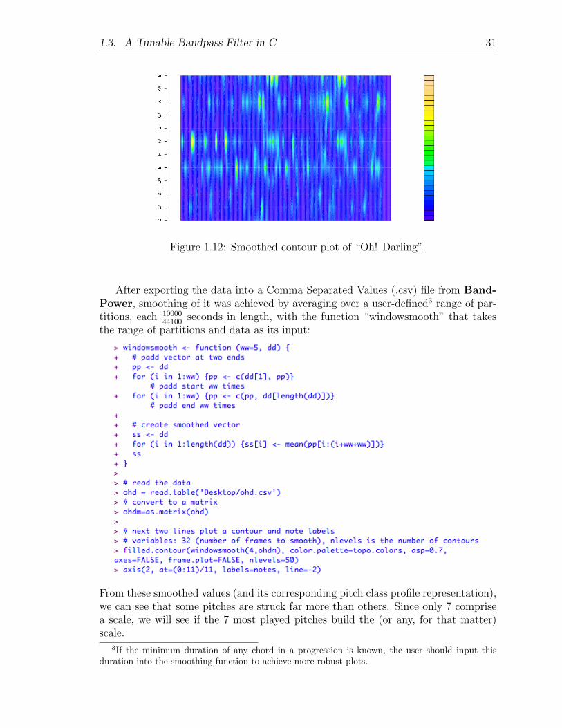
Since it is so hard to find an actual triad that makes it to the three most powerfulfrequencies, I decided to smooth the data and see if meaningful chords would evolvethen. The entirety of “Oh! Darling,” unsmoothed and then smoothed in the programR, is depicted in Figures 1.11 and 1.12. These colorful graphs are known as PitchClass Profiles, in which the y-axis shows “pitch class” (one of C through B), thex-axis is time, and the entries are the individual powers. Those with little to no powerare colored dark blue, and those with some to a lot of power are tinted somewherebetween green and orange. This graphical system, developed by Fujishima in 1999, isa powerful way of visualizing the harmony of a song because it is three-dimensional.It is clearly much easier to understand and conjecture about the chord progressionfrom the smoothed contour map versus the unsmoothed one.
Figure 1.11: Unsmoothed contour plot of “Oh! Darling”.
1.3. A Tunable Bandpass Filter in C 31
Figure 1.12: Smoothed contour plot of “Oh! Darling”.
After exporting the data into a Comma Separated Values (.csv) file from Band-Power, smoothing of it was achieved by averaging over a user-defined3 range of par-titions, each 10000
44100seconds in length, with the function “windowsmooth” that takes
the range of partitions and data as its input:
From these smoothed values (and its corresponding pitch class profile representation),we can see that some pitches are struck far more than others. Since only 7 comprisea scale, we will see if the 7 most played pitches build the (or any, for that matter)scale.
3If the minimum duration of any chord in a progression is known, the user should input thisduration into the smoothing function to achieve more robust plots.
32 Chapter 1. Automatic Recognition of Digital Audio Signals
1.3.2 Key Detection
Because the majority of humans do not have perfect pitch, intervals of two notes soundthe same regardless of their location on the keyboard. For example, the interval of 5half steps known as a perfect fourth (P4) sounds the same whether between an A andD, or a G and C. To account for this aural normalization, we write chords as Romannumerals relative to their key, where “I” and “i” both occur on the first scale degree4
(the tonic), “ii” and “iio” on the second degree of the scale (the supertonic), andso on. The notation “[ II” means that the chord is rooted at a half step above thefirst scale degree and a half step below the second scale degree. The seven “ordinary”triads within a major key are labeled I, ii, iii, IV, V, vi, and viio, where a capitalizedRoman numeral indicates a major quality, i.e., the second note in the chord is 4 halfsteps above the root and the third note in the chord is 7 half steps above the root.A lowercase Roman numeral indicates a minor quality, where the second note is 3half steps above the root and the third is also 7 half steps above the root. Finally,a lowercase Roman numeral followed by a “o” indicates a diminished chord quality,where the second note is 3 half steps above the root and the third is 6 half steps awayfrom the root.
The natural triads in a minor key are i, iio, III, iv, v, IV, and VII. If you takea moment to look at the pattern of qualities of the chords in the minor key lineupagainst that of the major key, you’ll see that the minor key begins on the sixth scaledegree of a major key. This major key is called its relative major key because thenotes are the same.
When we are in a major key but encounter a chord like v, we say it is borrowingfrom the parallel minor key, for the root is the same but the scale degrees are indifferent places (i.e., G Major and g minor are in a parallel-key relationship). It isvery common for both major and minor keys to borrow chords from their relativecounterparts, in the Beatles’ and Beethoven’s music alike. In fact, I wish I hadaccounted for this common event in my analysis and naming with Roman numerals,by saying that every song is in a major key, since the chords can simply be writtenvi, viio, I, etc. instead of i, iio, III. That way, the behavior of major and minor songscould be analyzed together, and the labeling would be normalized.
When we encounter a chord that is neither in the major or parallel minor scale,we consider two things before labeling it with a Roman numeral. First, we analyzeits quality. If it is a major chord, we check to see if its root is at [2, in which caseit is the Neapolitan chord. Otherwise, we label it with a “V/” and see what note is7 half steps below its root, and put the appropriate Roman numeral from our key(or its parallel key) underneath this slash. Most of these chords, called secondarydominants, transition next to the chord underneath the V. This is called resolution.For instance, V/iii (consisting of the scale degrees 7, ]2, and ]4) “resolves” to thechord iii (consisting of 3, 5, and 7). But in modern music, this is not as strict of arule as it was in classical compositions, so we will label a chord constructed with 7,]2, and ]4 as a V/iii even if it does not resolve to iii.
Now, summing the powers of each pitch in the song “Oh! Darling,” we calculate
4See glossary.
1.3. A Tunable Bandpass Filter in C 33
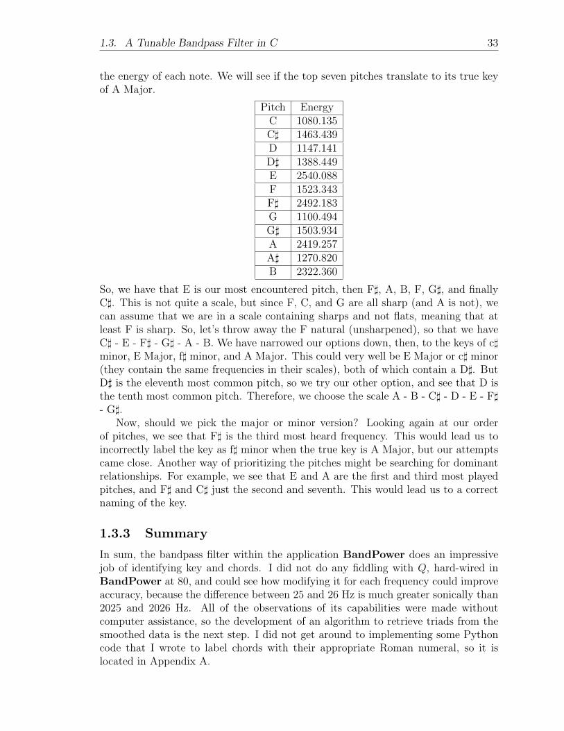
the energy of each note. We will see if the top seven pitches translate to its true keyof A Major.
Pitch EnergyC 1080.135C] 1463.439D 1147.141D] 1388.449E 2540.088F 1523.343F] 2492.183G 1100.494G] 1503.934A 2419.257A] 1270.820B 2322.360
So, we have that E is our most encountered pitch, then F], A, B, F, G], and finallyC]. This is not quite a scale, but since F, C, and G are all sharp (and A is not), wecan assume that we are in a scale containing sharps and not flats, meaning that atleast F is sharp. So, let’s throw away the F natural (unsharpened), so that we haveC] - E - F] - G] - A - B. We have narrowed our options down, then, to the keys of c]minor, E Major, f] minor, and A Major. This could very well be E Major or c] minor(they contain the same frequencies in their scales), both of which contain a D]. ButD] is the eleventh most common pitch, so we try our other option, and see that D isthe tenth most common pitch. Therefore, we choose the scale A - B - C] - D - E - F]- G].
Now, should we pick the major or minor version? Looking again at our orderof pitches, we see that F] is the third most heard frequency. This would lead us toincorrectly label the key as f] minor when the true key is A Major, but our attemptscame close. Another way of prioritizing the pitches might be searching for dominantrelationships. For example, we see that E and A are the first and third most playedpitches, and F] and C] just the second and seventh. This would lead us to a correctnaming of the key.
1.3.3 Summary
In sum, the bandpass filter within the application BandPower does an impressivejob of identifying key and chords. I did not do any fiddling with Q, hard-wired inBandPower at 80, and could see how modifying it for each frequency could improveaccuracy, because the difference between 25 and 26 Hz is much greater sonically than2025 and 2026 Hz. All of the observations of its capabilities were made withoutcomputer assistance, so the development of an algorithm to retrieve triads from thesmoothed data is the next step. I did not get around to implementing some Pythoncode that I wrote to label chords with their appropriate Roman numeral, so it islocated in Appendix A.

Chapter 2
Markovian Probability Theory
This temporal world is filled with events that depend on the past. Nearly everypresent manifestation of human behavior is based on what one has learned frommistakes and successes from the past, appearing to approach some optimal limit afterenough time has passed. Markovian processes characterize events that happen insequence, and models their local behavior with a matrix.
The hidden Markov model (HMM) is used when we want to predict the behavior ofa data set, and we are not sure of how to exactly characterize its prior behavior. Thus,we build a Markov chain based on previous observations of the action or set of actionswe wish to predict, whether the stock market, or the weather, or one’s health—or,here, the typical chord progression of a style, or region, or artist, or album, and thenwe can produce guesses for future observations, given that the model is not completelyrandom. Will Landecker studied HMMs and attempted to compose a new, Bach-likemelody using data from one of Bach’s works, Minuet in G. My project aims not tocompose music from my data, but to study the difference in the models constructedfrom various pools of songs, so it just involves counting up the number of times wetransition from chord to chord, and dividing by the total sum of chords to find aprobability, instead of the complex algorithms involved with hidden Markov models.For instance, I would like to know the difference between Irving Berlin’s and ColePorter’s songs, so I create two chains from their bodies of work, thereby forming two(presumably distinct) transition matrices, and subtract the two matrices. But whenI want to look at more than two models, another measure of comparison must bemade. Hence, I look at the entropy of the system, since it measures uncertainty. Wewill look at the meaning derived from the subtraction versus that derived from themeasure of entropy, and decide if entropy is indeed a good indicator of style, relativeto other styles, in music.
For more on hidden Markov models and their application to automatic speech(and chord) recognition, see Appendix B.
36 Chapter 2. Markovian Probability Theory
2.1 Probability Theory
The idea of Markovian processes is easily relatable and accessible in the real world ofchoices and decision-making, like much of the notions enveloped by probability theory:a Markov chain describes the probability of some state sj occurring next given thatwe are “in” state si with a matrix that contains this probability in the (i, j)th entry.This can be thought of as the probability that it will rain tomorrow (state sj), orany other designated period of time, given that it is raining today (states si = sj), orthe probability that it will not rain tomorrow (state sj) given that it is not rainingtoday (states si 6= sj), and so on, to describe 4 total transition probabilities. Say theprobability of it raining tomorrow, given rain today, is 0.7, and the probability that itwill rain tomorrow given that it is not raining today is 0.2. Then we can infer that theprobability of it not raining tomorrow given that it is raining today is 1− 0.7 = 0.3,and the probability of no rain tomorrow given no rain today is 1− 0.2 = 0.8. This isvisualizable with a transition matrix:
A =
[0.8 0.20.3 0.7
]The entry aij, 1 ≤ i, j ≤ 2 is the probability of going from state si to state sj, so here,state s1 is the case in which it is not raining, and state s2 is the case in which it israining. Note that the rows of A must sum to 1 if the state appears in the Markovchain at any point before time t = T . Otherwise, the rows sum to 0.
Now, if this data did not exist somewhere, we would have to count it up our-selves from some subset of observations of the weather, and build these probabilitiesourselves. This is the naıve version of a Hidden Markov Model, and we leave the al-gorithmic one to be explained in Appendix B. The naıve version is more manageablewhen we do not need to compare our observations with our expectations. Because weonly have a little intuition on the abstract nature of quantifying musical harmony, wecan describe our expectations qualitatively, and test our results by experimentation.
Before we get too far into Markov chains, however, let us review some essentialparts of probability theory [5] that will help our intuitions on the subject.
Definition: Discrete-Time Random Variable. A real-valued variable X is adiscrete-time random variable if it can only take on at most a countable numberof possible values si for all arguments t of X, 0 ≤ t ≤ T , t, T ∈ N. We call the set ofthese possible values that X can take on the state space S of X, |S| = N ≤ T . Wecan formally define the function X by
X : N→ S.
For example, say that our state space consisted of 24 major and minor chords, andwe ordered them so that s1 = C Major and sN = s24 = b minor. Then, the randomvariable X would map each point in time to one of these chords, with replacement(i.e., it could be the case that X(t) = X(t′) = s1 = C Major, for t 6= t′). This makesit clear that it is not necessarily true that X(1) = s1; X(1) could be any value of S.
2.1. Probability Theory 37
Definition: Discrete-Time Random Process. A discrete-time randomprocess
X(0), X(1), . . . , X(T )
is an ordered sequence of real, positive integer values corresponding to the value of therandom variable X at time t. We say that X(t) is in state si at time t iff X(t) = si,1 ≤ i ≤ N , i, t, T,N ∈ N.
Definition: Event. We define an event E to be any set of outcomes in S, such asthe event that the sum of the two dice is 7, in which caseE = (1, 6), (2, 5), (3, 4), . . . ⊆S, and (1, 6) is an outcome ei ∈ S. The union of all the events in S equals S. Whenwe define events such that they are disjoint, the sum of the probabilities of all theevents is 1.
Definition: Independence. Two events or outcomes in S are independentif the probability of one of them occurring does not influence the probability of theother occurring.
For example, when we toss a die, whether it is weighted or unweighted (“fair”), itsoutcome is not influenced by previous outcomes. There are few real world examplesin which the outcomes are independent of each other.
Definition: Conditional Probability. The conditional probability of eventF occurring given that E occurred is given by the following formula:
P (F |E) =P (EF )
P (E)
for P (E) > 0. We consider the concept of conditional probability to be the oppositeof independence, since when E and F are independent, P (F |E) = P (F ).
Keeping our example of the sum of two dice, let E be the event (outcome) inwhich the first die equals 2. What, then, is the probability of the sum of that die’soutcome plus that of another die yet to be rolled equals 8? It is simply P (second die
is 6) = 16, which is not equal to P (sum of two dice is 8) = |(2,6),(3,5),(4,4),(5,3),(6,2)|
|S| = 536
.
Definition: Bayes’ Formula. Suppose that F1, F2, . . . , Fn are mutually exclu-sive (disjoint) events such that
n⋃i=1
Fi = S,
i.e., exactly one of the events Fi must occur. Define E by
E =n⋃i=1
EFi,
38 Chapter 2. Markovian Probability Theory
and note that the events EFi themselves are mutually exclusive. Then we obtain
P (E) =n∑i=1
P (EFi)
=n∑i=1
P (E|Fi)P (Fi).
In other words, we can compute P (E) by first conditioning on the outcome Fi. Sup-pose now that E has occurred and we are interested in determining the probabilitythat Fj also occurred. This is the premise of Bayes’ formula, which is as follows:
P (Fj|E) =P (EFj)
P (E)
=P (E|Fj)P (Fj)∑ni=1 P (E|Fi)P (Fi)
.
This formula may be interpreted as evidencing how the “hypotheses” P (Fj) shouldbe modified given the conclusions of our “experiment” E.
Definition: Probability Mass Function. For a discrete-time random variableX, we define the probability mass function p(x)
for x ∈ R, p(x) = Pt ∈ N : X(t) = x.
The probability mass function (pmf) is positive for at most a countable number ofvalues of x, since X is discrete. Since X must take on one of the values x, we have∑
x∈X
p(x) = 1.
The distribution function F(x) of X is similar in that it finds the probability thatthe random variable is less than or equal to x, and is defined by
F (x) = Px ∈ R : X ≤ x =x∑
y=−∞
p(y),
and is also referred to as the cumulative distribution function or cdf of X. It isnondecreasing, such that Pa ≤ X ≤ b = F (b)− F (a) is nonnegative.
Definition: Expectation. If X is a discrete random variable having a probabil-ity mass function p(x), the expectation or the expected value of X, denoted byE[X], is defined by
E[X] =∑
x:p(x)>0
x p(x),
2.2. Markov Chains 39
where the x’s are the values that X takes on. This can be thought of as a weightedaverage of the state space S.
For example, flipping a fair coin heeds the probability mass function p(heads)= 1
2= p(tails), so we could write
p(0) =1
2= p(1)
E[X] = 0
(1
2
)+ 1
(1
2
)=
1
2.
Definition: Finite Probability Scheme. A finite probability scheme E ofthe sample space S is a partition of S into disjoint events Ei with probabilities thatsum to 1, represented by the array
S =
[E1 E2 . . . Enp1 p2 . . . pn
]where n is the number of parts in the partition of S, and pi is the probability of eventEi,
∑ni=1 pi = 1.
Each event Ei has its own set of individual outcomes, which can be thought ofas elementary events (events with cardinality 1), written e1, . . . , em with probabilities∑m
j=1 p(ej) = 1 as well.
2.2 Markov Chains
Now that we have laid the framework for the terminology used in defining our hiddenMarkov models, we can continue to a formal definition of a Markov chain, and tothe properties they exhibit. Here, we will use the notation (X0, . . . , XT ) in place ofX(0), . . . , X(T ), only because it is widespread.
Definition: Markov Property. If the conditional distribution of the variableXt+1, given the process (X0, X1, . . . , Xt), where Xi is some state such as a rain onday i, depends only on the previous variable, Xt, i.e.,
p(Xt+1|X0, . . . , Xt) = p(Xt+1|Xt),
the process is said to satisfy the memoryless property, or Markov property.
The word “depends” here is somewhat misleading. Independent outcomes can bemodeled by a Markov chain: then, p(Xt+1|Xt) = p(Xt+1). Therefore, two consecutivestates do not necessarily have to be related to write them as a conditional probability.
40 Chapter 2. Markovian Probability Theory
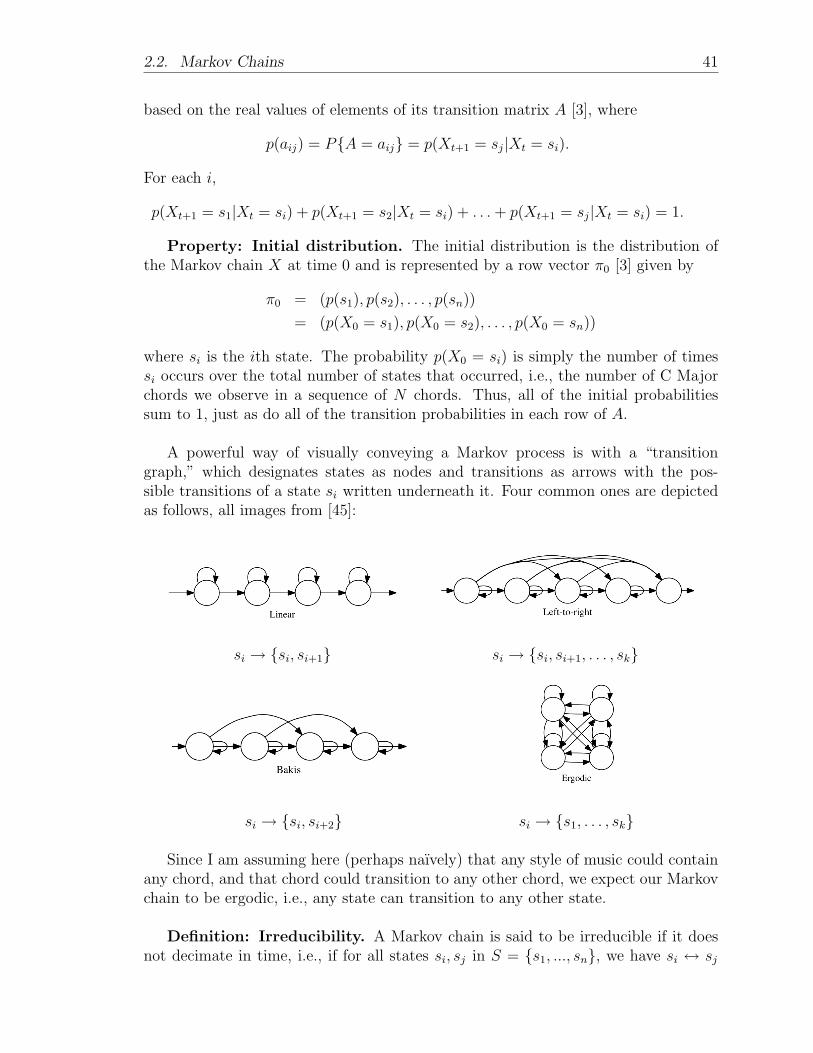
Instinctively, Markov chains possess the Markov property. They can be “homoge-neous,” “irreducible,” “aperiodic,” and “stationary,” all of which are defined below.Hidden Markov models are “time-homogeneous,” which means that the probabilityof transitioning between two given states does not change over time. Hence, evenwhen we observe a sequence of four heads from a fair coin, the probability of flippinga head next is still 0.5.1
Although music is much like speech in its grammar-like structure, two musiciansactually differ less than two speakers in their spectrograms. Therefore, there is noneed to waste time constructing a whole hidden Markov model for our data since theF] from a piano does not differ drastically from the F played from a guitar. For moreon hidden Markov models, see Appendix B.
Now we have arrived at our definition of a Markov chain. We call our set of chordsthe “state space” S2, and our chord progression an ordered sequence X of chords inS from time t = 0 to t = T . We record the transition probabilities in an |S| × |S|matrix A.
Definition: Markov Chains. Let A be a n×n matrix with real-valued elementsaij : i, j = 1, . . . , n, all of which are nonnegative and sum to 1. A random process(X0, . . . , XT ) with values from the finite state space S = s1, . . . , sn is said to be aMarkov chain with transition matrix A, if, for all t, i, and k such that 0 ≤ t ≤ T, 1 ≤i, j, i0, i1, . . . , ik ≤ n
p(Xt+1 = sj|X0 = si0 , . . . , Xt−1 = sik , Xt = si) = p(Xt+1 = sj|Xt = si)
= aij,
Thus, aij is the transition probability of moving from state si to state sj.
More specifically, this is a time-homogeneous Markov chain, since, from onetime to another, the transition probabilities do not change.
In other words, a Markov chain is a random process usually governed by some-thing that cannot be concretely understood, like the weather governs rain or harmonygoverns music. Harmony in music can come from unexpected aspects, like new chordsthat have rarely been played before or thunderstorms in Oregon, and that is why weconsider this and other Markov chains random processes. Note that just because itis random does not mean there do not exist patterns that we can identify after thefact—in other words, it can still contain conditional probabilities, but the weathertomorrow does not necessarily abide by those conditional probabilities. Rather, thecharacter of the newly observed state of the weather is added to the Markov chain,and the transition probabilities are then updated.
Property: Probability mass function. X has its probability mass function
1Since we do classify music by the era from which it comes, our hidden Markov model is not time-homogeneous, and is instead “state-homogeneous,” since there are only a finite number of possiblestates.
2In section 2.2.1, Song as a Probability Scheme, we call the state space C.
2.2. Markov Chains 41
based on the real values of elements of its transition matrix A [3], where
p(aij) = PA = aij = p(Xt+1 = sj|Xt = si).
For each i,
p(Xt+1 = s1|Xt = si) + p(Xt+1 = s2|Xt = si) + . . .+ p(Xt+1 = sj|Xt = si) = 1.
Property: Initial distribution. The initial distribution is the distribution ofthe Markov chain X at time 0 and is represented by a row vector π0 [3] given by
π0 = (p(s1), p(s2), . . . , p(sn))
= (p(X0 = s1), p(X0 = s2), . . . , p(X0 = sn))
where si is the ith state. The probability p(X0 = si) is simply the number of timessi occurs over the total number of states that occurred, i.e., the number of C Majorchords we observe in a sequence of N chords. Thus, all of the initial probabilitiessum to 1, just as do all of the transition probabilities in each row of A.
A powerful way of visually conveying a Markov process is with a “transitiongraph,” which designates states as nodes and transitions as arrows with the pos-sible transitions of a state si written underneath it. Four common ones are depictedas follows, all images from [45]:
si → si, si+1 si → si, si+1, . . . , sk
si → si, si+2 si → s1, . . . , sk
Since I am assuming here (perhaps naıvely) that any style of music could containany chord, and that chord could transition to any other chord, we expect our Markovchain to be ergodic, i.e., any state can transition to any other state.
Definition: Irreducibility. A Markov chain is said to be irreducible if it doesnot decimate in time, i.e., if for all states si, sj in S = s1, ..., sn, we have si ↔ sj
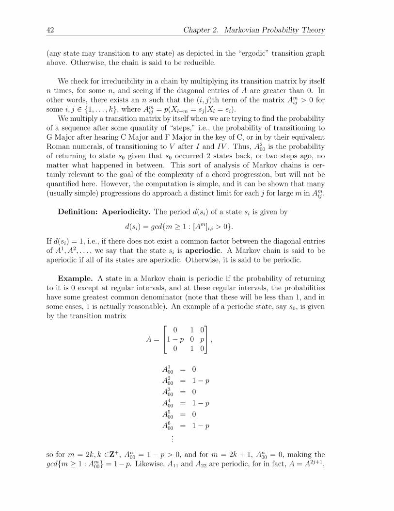
42 Chapter 2. Markovian Probability Theory
(any state may transition to any state) as depicted in the “ergodic” transition graphabove. Otherwise, the chain is said to be reducible.
We check for irreducibility in a chain by multiplying its transition matrix by itselfn times, for some n, and seeing if the diagonal entries of A are greater than 0. Inother words, there exists an n such that the (i, j)th term of the matrix Amij > 0 forsome i, j ∈ 1, . . . , k, where Amij = p(Xl+m = sj|Xl = si).
We multiply a transition matrix by itself when we are trying to find the probabilityof a sequence after some quantity of “steps,” i.e., the probability of transitioning toG Major after hearing C Major and F Major in the key of C, or in by their equivalentRoman numerals, of transitioning to V after I and IV . Thus, A2
00 is the probabilityof returning to state s0 given that s0 occurred 2 states back, or two steps ago, nomatter what happened in between. This sort of analysis of Markov chains is cer-tainly relevant to the goal of the complexity of a chord progression, but will not bequantified here. However, the computation is simple, and it can be shown that many(usually simple) progressions do approach a distinct limit for each j for large m in Amij .
Definition: Aperiodicity. The period d(si) of a state si is given by
d(si) = gcdm ≥ 1 : [Am]i,i > 0.
If d(si) = 1, i.e., if there does not exist a common factor between the diagonal entriesof A1, A2, . . . , we say that the state si is aperiodic. A Markov chain is said to beaperiodic if all of its states are aperiodic. Otherwise, it is said to be periodic.
Example. A state in a Markov chain is periodic if the probability of returningto it is 0 except at regular intervals, and at these regular intervals, the probabilitieshave some greatest common denominator (note that these will be less than 1, and insome cases, 1 is actually reasonable). An example of a periodic state, say s0, is givenby the transition matrix
A =
0 1 01− p 0 p
0 1 0
,A1
00 = 0
A200 = 1− p
A300 = 0
A400 = 1− p
A500 = 0
A600 = 1− p...
so for m = 2k, k ∈Z+, An00 = 1 − p > 0, and for m = 2k + 1, An00 = 0, making thegcdm ≥ 1 : Am00 = 1− p. Likewise, A11 and A22 are periodic, for in fact, A = A2j+1,
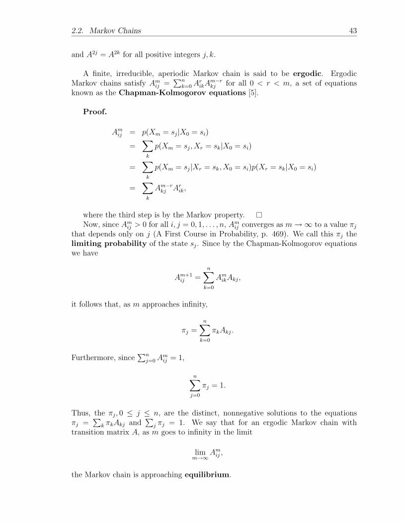
2.2. Markov Chains 43
and A2j = A2k for all positive integers j, k.
A finite, irreducible, aperiodic Markov chain is said to be ergodic. ErgodicMarkov chains satisfy Amij =
∑nk=0A
rikA
m−rkj for all 0 < r < m, a set of equations
known as the Chapman-Kolmogorov equations [5].
Proof.
Amij = p(Xm = sj|X0 = si)
=∑k
p(Xm = sj, Xr = sk|X0 = si)
=∑k
p(Xm = sj|Xr = sk, X0 = si)p(Xr = sk|X0 = si)
=∑k
Am−rkj Arik,
where the third step is by the Markov property.Now, since Amij > 0 for all i, j = 0, 1, . . . , n, Amij converges as m→∞ to a value πj
that depends only on j (A First Course in Probability, p. 469). We call this πj thelimiting probability of the state sj. Since by the Chapman-Kolmogorov equationswe have
Am+1ij =
n∑k=0
AmikAkj,
it follows that, as m approaches infinity,
πj =n∑k=0
πkAkj.
Furthermore, since∑n
j=0Amij = 1,
n∑j=0
πj = 1.
Thus, the πj, 0 ≤ j ≤ n, are the distinct, nonnegative solutions to the equationsπj =
∑k πkAkj and
∑j πj = 1. We say that for an ergodic Markov chain with
transition matrix A, as m goes to infinity in the limit
limm→∞
Amij ,
the Markov chain is approaching equilibrium.
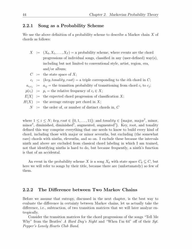
44 Chapter 2. Markovian Probability Theory
2.2.1 Song as a Probability Scheme
We use the above definition of a probability scheme to describe a Markov chain X ofchords as follows:
X := (X0, X1, . . . , XT ) = a probability scheme, where events are the chord
progressions of individual songs, classified in any (user-defined) way(s),
including but not limited to conventional style, artist, region, era,
and/or album;
C := the state space of X;
ci := (key, tonality, root) = a triple corresponding to the ith chord in C;
acicj := aij = the transition probability of transitioning from chord ci to cj;
p(ci) := pi = the relative frequency of ci ∈ X;
E[X] := the expected chord progression of classification X;
H(X) := the average entropy per chord in X;
N := the order of, or number of distinct chords in, C
where 1 ≤ i ≤ N ; key, root ∈ 0, 1, . . . , 11; and tonality ∈ major, major7, minor,minor7, diminished, diminished7, augmented, augmented7. Key, root, and tonalitydefined this way comprise everything that one needs to know to build every kind ofchord, including those with major or minor sevenths, but excluding (the somewhatrare) chords with ninths, elevenths, and so on. I exclude these because the intervalsninth and above are excluded from classical chord labeling in which I am trained,not that identifying ninths is hard to do, but because frequently, a ninth’s functionis that of an accidental.
An event in the probability scheme X is a song Xk with state space Ck ⊆ C, buthere we will refer to songs by their title, because there are (unfortunately) so few ofthem.
2.2.2 The Difference between Two Markov Chains
Before we assume that entropy, discussed in the next chapter, is the best way toevaluate the difference in certainty between Markov chains, let us actually take thedifference, i.e., subtraction, of two transition matrices that we will later analyze en-tropically.
Consider the transition matrices for the chord progressions of the songs “Tell MeWhy” from the Beatles’ A Hard Day’s Night and “When I’m 64” off of their Sgt.Pepper’s Lonely Hearts Club Band.
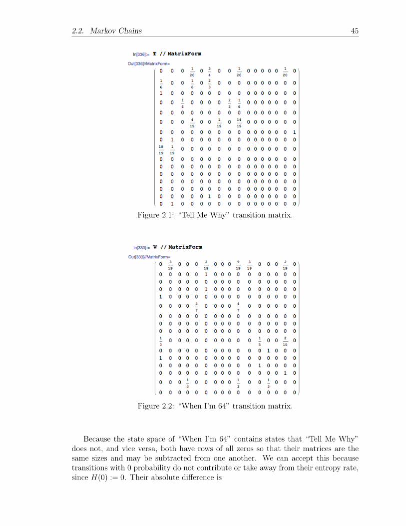
2.2. Markov Chains 45
Figure 2.1: “Tell Me Why” transition matrix.
Figure 2.2: “When I’m 64” transition matrix.
Because the state space of “When I’m 64” contains states that “Tell Me Why”does not, and vice versa, both have rows of all zeros so that their matrices are thesame sizes and may be subtracted from one another. We can accept this becausetransitions with 0 probability do not contribute or take away from their entropy rate,since H(0) := 0. Their absolute difference is
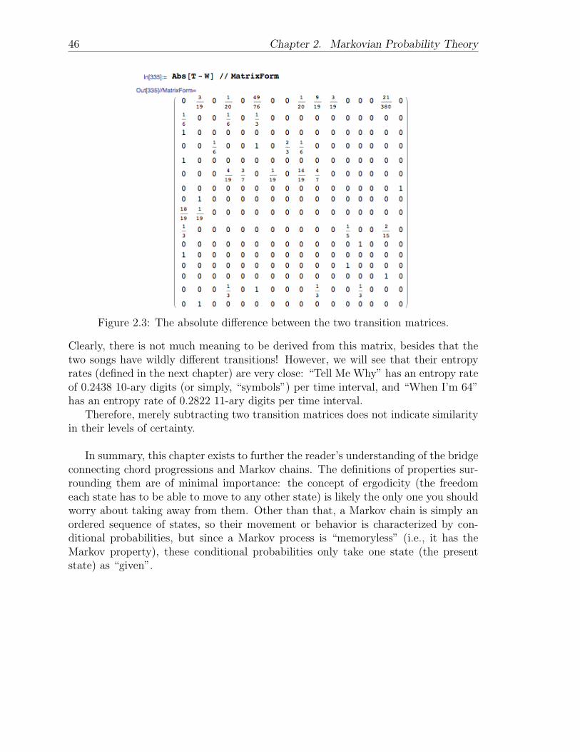
46 Chapter 2. Markovian Probability Theory
Figure 2.3: The absolute difference between the two transition matrices.
Clearly, there is not much meaning to be derived from this matrix, besides that thetwo songs have wildly different transitions! However, we will see that their entropyrates (defined in the next chapter) are very close: “Tell Me Why” has an entropy rateof 0.2438 10-ary digits (or simply, “symbols”) per time interval, and “When I’m 64”has an entropy rate of 0.2822 11-ary digits per time interval.
Therefore, merely subtracting two transition matrices does not indicate similarityin their levels of certainty.
In summary, this chapter exists to further the reader’s understanding of the bridgeconnecting chord progressions and Markov chains. The definitions of properties sur-rounding them are of minimal importance: the concept of ergodicity (the freedomeach state has to be able to move to any other state) is likely the only one you shouldworry about taking away from them. Other than that, a Markov chain is simply anordered sequence of states, so their movement or behavior is characterized by con-ditional probabilities, but since a Markov process is “memoryless” (i.e., it has theMarkov property), these conditional probabilities only take one state (the presentstate) as “given”.
Chapter 3
Information, Entropy, and Chords
3.1 What is information?
The study of communication requires certain statistical and probabilistic parametersthat the theory of information provides. Many consider the mathematical definitionof information unintuitive. Indeed, information and uncertainty have a directly pro-portional relationship: the more that is left up to chance in a message, the more infor-mation a message must contain in order to be transmitted unambiguously. However,they are in fact opposites, because the more uncertain a message, the less informationit contains. For compression purposes as well as efficient coding methods, knowinghow much information is contained in a given message is highly relevant and vital todeveloping a well-functioning model.
Unary is the simplest language for humans and computers alike to “speak”. It isalso the least efficient. If we communicated in unary, where our language was only“0” (permitting a space bar), every distinct word in our language would be translatedto a distinct length of 0’s. Therefore, binary is the second simplest, but with it wecan actually communicate in half the amount of total symbols. We use binary digits(and the base-2 logarithm) exclusively when we talk about information theory.
Consider a string of independent binary digits. We should treat it as a queue ofsymbols where each has one of two actions, one with probability p, and the other withprobability 1− p. There are two possibilities, 0 and 1, for each symbol in the string,and 2N possible strings, where N is the length of the string. Since a symbol, if not 0,is 1, each symbol’s identity can be realized with only one (binary) question: “Is thedigit a 0?” Therefore, there are at most log2(2
N) = N yes/no questions required touniquely identify each string.
Claude Shannon discusses the encoding of the English alphabet in his transcen-dental work, The Mathematical Theory of Communication (1948). Counts are madefrom some given set of text, say a dictionary, to see the relative frequencies of theletters ’e’ and ’a’ versus ’z’ or ’x’. Noting that ’e’ is one of the more common symbols,we would want to represent it with a shorter string of code than one we might choosefor ’z’ or ’x’, the least occurring symbols, so that a message could be transmitted asquickly as possible.
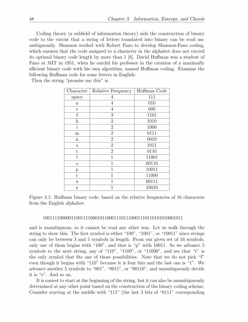
48 Chapter 3. Information, Entropy, and Chords
Coding theory (a subfield of information theory) aids the construction of binarycode to the extent that a string of letters translated into binary can be read un-ambiguously. Shannon worked with Robert Fano to develop Shannon-Fano coding,which ensures that the code assigned to a character in the alphabet does not exceedits optimal binary code length by more than 1 [6]. David Huffman was a student ofFano at MIT in 1951, when he outdid his professor in the creation of a maximallyefficient binary code with his own algorithm, named Huffman coding. Examine thefollowing Huffman code for some letters in English:Then the string “promise me this” is
Character Relative Frequency Huffman Codespace 4 111
a 4 010e 4 000f 3 1101h 2 1010i 2 1000
m 2 0111n 2 0010s 2 1011t 2 0110l 1 11001o 1 00110p 1 10011r 1 11000u 1 00111x 1 10010
Figure 3.1: Huffman binary code, based on the relative frequencies of 16 charactersfrom the English alphabet.
10011110000011001111000101100011101110001110110101010001011
and is unambiguous, so it cannot be read any other way. Let us walk through thestring to show this. The first symbol is either “100”, “1001”, or “10011” since stringscan only be between 3 and 5 symbols in length. From our given set of 16 symbols,only one of them begins with “100”, and that is “p” with 10011. So we advance 5symbols to the next string, any of “110”, “1100”, or “11000”, and see that “r” isthe only symbol that fits one of those possibilities. Note that we do not pick “f”even though it begins with “110” because it is four bits and the last one is “1”. Weadvance another 5 symbols to “001”, “0011”, or “00110”, and unambiguously decideit is “o”. And so on.
It is easiest to start at the beginning of the string, but it can also be unambiguouslydetermined at any other point based on the construction of the binary coding scheme.Consider starting at the middle with “111” (the last 3 bits of “0111” corresponding
3.1. What is information? 49
to “m”) and deciding that is “space”. The next is either “000”, “0001”, or “00011”,and we decide it is “e” (mapped to “000”). Then the previous string is any of “110”,“1110”, or “01110”, and we realize that this does not correspond to any of the binarycodes assigned to our given vocabulary, so our initial starting point was not at thebeginning of a symbol’s code.
Huffman developed his encoding methods such that any set of symbols (not just16, although the fact that 16 is a power of 2 does contribute to the maximal efficiencyof the given encoding scheme) could be assigned unambiguous bit representations,enabling shorter signals that do not utilize all 27 characters of the English alphabet tobe transmitted even faster—in fact, as briefly as binary will allow. In this way, entropymeasures the compressibility of a set of symbols, when we know the probability ofcorrectly transmitting them.
In this thesis, the letters of our alphabet will be pitches, such that the cardinalityof our alphabet is 12. Therefore, words are chords, sentences are musical phrases,and paragraphs are an entire song. We could extend the idea of supersets in musicalclassification even further, chapters to albums, books to discographies, but there itgets a little fuzzy1.
Information theory and logarithms have a deeply seeded connection, namely withinthe function of entropy. Entropy is the uncertainty, or information, contained in amessage. It is a measure of the likeliness that a sent message will not convey theintended meaning it was given, and it is equal to the number of bits2 per symbol ofimprobability that the message contains. It follows that a scenario in which all of theevents are independent and equally likely contains the most entropy of any scenario,for there are the most possible messages: if you wanted to transmit a “6” from tossinga fair die, there would only be a 1/6 probability of that happening.
To further color this important characteristic, consider a probability scheme Awith outcomes A1 and A2, say heads and tails, p(A1) = p(A2) = 1
2. Also, say that
we are transmitting these H’s and T’s at 1000 symbols per second3. If we want totransmit the sequence “HTHH”, in a model where H and T are transmitted withthe same probability and they are the only symbols we can transmit, the sequence“HTHH” is just as likely to be transmitted as “THTT” or “THHT” or any sequenceof 4 symbols. Thus, we expect only half of the symbols to be transmitted correctly,left entirely up to chance (entropy), so we say that our source is actually transmitting0 bits of information (i.e., the certainty that the transmitted symbol was the one thesource intended to transmit). This is the same as calculating −
(12
log212
+ 12
log212
)=
−(
12· −1 + 1
2· −1
)= 1 bit/symbol, and multiplied by our transmission rate of 1000
symbols/second is 1000 bits/second. Our given message and the resulting messageafter going through this probabilistic encoding process work against each other, so
1We could also call chords phonemes or morphemes, as in linguistics, because they contributeto the meaning/emotion of a song, as well as are designed keeping the restrictions of the apparatus(instrument) in mind.
2John Tukey’s shortening of “binary digit” [6]3What would the transmission rate of music be? If you find yourself asking this, observe that a
“rate” implies that is only a scaling factor, and therefore the entropy rate is all that is importanthere.
50 Chapter 3. Information, Entropy, and Chords
we subtract this rate from our transmission rate to determine how much informationis actually being processed, which is 1000− 1000 = 0 bits/symbol as we expected [6].
Now, for a probability scheme B, also with 2 outcomes B1 and B2 such thatp(B1) = 0.99 and p(B2) = 0.01, we would expect our system to transmit informationat a high rate, and have low entropy. We might guess that the transmission ofinformation would have a rate of 990 bits/second, but this does not take into accountthe independence of the symbols and replacement. We find that the entropy is equalto −
∑2i=1 p(Bi) log2 p(Bi) = − (0.99 log2 0.99 + 0.01 log2 0.01) = 0.081 bits/symbol,
multiplied by our sampling rate is 81 bits per second, and see that the system isactually transmitting at 1000− 81 = 919 bits/second of information.
This is the independent case, at least. It is rare that two events in this world,however, are unrelated to each other. Therefore, it is even more rare for the tth symbolin a sequence to be independent of what came before (the first through (t − 1)stsymbols, or perhaps, as in Markovian processes, just the (t − 1)st symbol), andthrough this we can transcribe any sort of progression for the purpose of effectivecommunication, in some harmonic and witty arrangement. The words of a singlestatement can be jumbled up to the point of nonsense, but together, their meaning islikely still translatable. But, like intelligent and correct speech, the genius of music liesin perfectly aligned rhythm between the melodic line and lyric, the synthesis of severalinstruments or occasionally the choice to go solo, and, the most easily analyzablecharacteristic, the clever patterning of harmony to structure the aforementioned.
So, by nature, it is more interesting to look at cases involving conditional or jointprobabilities. When we want some way of probabilistically describing our Markovchain, information theory chimes in with many measures and applications to coding.Entropy is one of these measures. It is interesting to compare the entropies of differentsystems with one another, and see how distinct in “propensity for chaos” two systemsare. It is, in actuality, rather useless to look at the translation of this measure to itsbinary code-length, but the binary form does correspond to code containing howevermany symbols required to represent the number of chords in the vocabulary, say d, sothe measure we will find is easily scaled by log(2)
log(d). Therefore, it does not really matter
if we look at the binary interpretation or the d-ary one, for some positive integer d.For this reason, all logarithms used in this thesis, unless otherwise noted, are base-2and should be considered the “binary representation”.
3.2 The Properties of Entropy
First, we will remind the reader of the definition of a probability scheme, as statedin section 2.2.
Definition: Finite probability scheme. Given a finite sample space S, wedefine an event Ai ⊆ A ⊆ S to be any set of m outcomes a1, a2, . . . , am ∈ Ai withrespective probabilities p(aj) = qj,
∑j qj = 1. The probability of an event Ai is given
by p(Ai) = pi,∑n
i=1 pi = 1, where n is the number of events in A. The subsets Ai are
3.2. The Properties of Entropy 51
disjoint ∀i, and partition all of S [4]. We call the matrix
A =
[A1 A2 . . . Anp1 p2 . . . pn
]the finite probability scheme of S.4
As alluded to earlier, the function of entropy gives the average number of (binary)bits per symbol needed to correctly transmit a string of these symbols, where eachhas a given probability of being correctly transmitted. The following lengthy proofevolves the notion of entropy to the function H(X) = −
∑x∈X p(x) log p(x).
Theorem. Let H(p1, p2, ..., pn) be a function defined for any integer n and forall values p1, p2, . . . , pn, which are the probabilities of the subsets A1, A2, . . . , An in afinite probability scheme A such that pk ≥ 0 and
∑nk=1 pk = 1 . If, for any n, this
function is continuous ∀pi, and if
1. H is maximized when pk = 1n∀k (the characteristic we just showed);
2. For the product scheme AB, H(AB) = H(A) +H(B|A); and
3. H(p1, p2, . . . , pn, 0) = H(p1, p2, . . . , pn), i.e., adding an impossible event to ascheme does not change H;
then
H(A) = H(p1, p2, . . . , pn) = −λn∑k=1
pk log pk,
where λ is a positive constant.
Proof. Let H(
1n, 1n, . . . , 1
n
)= φ(n). We will show that φ(n) = λ log(n), where
λ > 0.Since H is maximized when pk = 1
n∀k by the first property, we have
φ(n) = H
(1
n,
1
n, . . . ,
1
n
)= H
(1
n,
1
n, . . . ,
1
n, 0
)≤ H
(1
n+ 1,
1
n+ 1, . . . ,
1
n+ 1,
1
n+ 1
)= φ(n+ 1),
4Note that it is possible for Ai = A, in which case the finite probability scheme features a1
through am in its first row and q1 through qm in its second.
52 Chapter 3. Information, Entropy, and Chords
i.e., φ is a non-decreasing function of n. Now, let m, r be positive integers. LetS1, S2, . . . , Sm be mutually exclusive schemes all containing r equally likely events,i.e., for all k,
H(Sk) = H
(1
r,1
r, . . . ,
1
r
)= φ(r).
Then, since all the schemes are independent by their disjointness,
H(S1S2) = H(S1) +H(S2)
= φ(r) + φ(r)
= 2 · φ(r)...
H(S1 · S2 · . . . · Sm) = H(S1) +H(S2) + . . .+H(Sm)
= m · φ(r).
But S1 · S2 · . . . · Sm (the “product scheme”) contains rm equally likely events, soH(S) = φ(rm). Hence,
φ(rm) = m · φ(r).
Now, let s and n be arbitrary numbers such that
rm ≤ sn ≤ rm+1.
Then
m log r ≤ n log s < (m+ 1) log rm
n≤ log s
log r<m+ 1
n.
Since φ is nondecreasing,
φ(rm) ≤ φ(sn) ≤ φ(rm+1)
which, because φ(rm) = m · φ(r), is equivalent to
m · φ(r) ≤ n · φ(s) ≤ (m+ 1) · φ(r)
m
n≤ φ(s)
φ(r)≤ (m+ 1)
n.
Then, since m+1n− m
n= 1
n, ∣∣∣∣φ(s)
φ(r)− log s
log r
∣∣∣∣ ≤ 1
n.
3.2. The Properties of Entropy 53
Since n is arbitrarily large,
φ(s)
log s=
φ(r)
log r
φ(r) =φ(s)
log slog r
= λ log r
where λ is a constant. Then
φ(n) = λ log n
by the arbitrariness of r and s. Since log n ≥ 0, and φ(n) ≥ 0, it is the case thatλ ≥ 0, and so we have proved our assertion.In fact, λ is simply the scalar log 2
log xfor a language with x symbols, because the log
function above is base-2.
To prove the general case, let A and B be two dependent schemes such that Aconsists of n events with probabilities p1, p2, ..., pn where
pk =gkg
(so, here it is not necessary that pk = 1n∀k), and
n∑k=1
gk = g,
and B consists of g events, which are divided into n subsets each containing gi events,1 ≤ i ≤ n. Then, for the event Ak ⊆ A, we have gk events in the kth group of B allwith a 1
gkprobability, and all other events in the 1st, 2nd, ... , (k-1)st, (k+1)st, ... ,
nth subsets of B have probability 0. Then
Hk(B) = H
(1
gk,
1
gk, ...,
1
gk
)= φ(gk)
= λ log gk.
54 Chapter 3. Information, Entropy, and Chords
Noting that the sum of all the pk is 1, this heeds the conditional entropy
H(B|A) =n∑k=1
gkgHk(B)
=n∑k=1
gkgλ log gk
= λn∑k=1
gkg
log g pk
= λ
n∑k=1
pk(log g + log pk)
= λ log g + λn∑k=1
pk log pk.
Now, consider the product scheme A · B = AB(= A ∩ B). The total number ofpossible events in AB is g, which is equal to the number of events in B, and sinceeach event is equally likely to occur,
pkgk
=1
g.
Therefore,
H(AB) = φ(g) = λ log g.
Now, by the second property, and from above,
H(AB) = H(A) +H(B|A)
= H(A) + λn∑k=1
pk log pk + λ log g.
Then we can subtract λ log g from both sides to get
0 = H(A) + λ
n∑k=1
pk log pk.
Thus,
H(A) = H(p1, . . . , pn)
= −λn∑k=1
pk log pk,
and we have arrived at the function of entropy. Since H is continuous by assumption,this holds for any value of pi. This completes the proof.
3.3. Different Types of Entropy 55
To recapitulate, we proved the functional form of entropy first for the maxi-mal case, when all the pi = 1
n. We did this mostly by the nondecreasing nature
of φ. Then, to prove the general case, we used the second property of H andthe conditional entropy (defined in the next section) H(B|A) to make the functionH(A) = −
∑nk=1 pk log pk to emerge (λ = 1 in the binary case).
Now let us backtrack and define H(B|A) and H(AB) more precisely.
3.3 Different Types of Entropy
Events where not all outcomes are independent of one another, as in a Markov chain,have different entropy than the independent case. All of these terms are defined forevents, but do extend to probability schemes.
3.3.1 Conditional Entropy
For simplicity of notation, we will write P (AB) to denote P (A ∩ B) and P (A · B).Recall that the conditional probability P (A|B), where the event A may or may notbe independent of event B, is
P (B|A) =P (AB)
P (A),
with the common notation of A ∩ B = AB demonstrated. When A and B are inde-pendent, i.e. disjoint, i.e. unrelated, P (B|A) = P (B).
Definition: Conditional Entropy. The conditional entropy of cj given ci,where ci and cj are distinct chords, is
H(cj|ci) = −p(cj)p(cj|ci) log p(cj|ci),
where p(ci) =∑n
k=0 p(ck)p(ci|ck), p(cj|ci) is the probability of transitioning from cito cj, and p(cj) is the probability of observing ci.
We will see in the definition of joint entropy that this quantity is also
H(cj|ci) = −p(ci, cj) log p(cj|ci),
i.e., p(ci, cj) = p(cj)p(cj|ci).Now, the conditional entropy H(D|ci), where C and D are events and |C| = m,
|D| = n, is conceptually the amount of entropy in D given the probability of onechord ci occurring.
H(D|ci) = −n∑j=1
p(dj|ci) log2 p(dj|ci)
56 Chapter 3. Information, Entropy, and Chords
and H(D|C) where the entirety of A is given is
H(D|C) = −m∑i=1
p(ci)H(D|C = ci)
= −m∑i=1
n∑j=1
p(ci)p(dj|ci) log2 p(dj|ci).
As in probability theory, C and D are mutually exclusive if and only if P (D|C) =P (D), so likewise,
(C ∪D) = ∅ ⇐⇒ H(D|C) = H(D).
It should follow intuitively that the conditional entropy when the events are dependentis always less than the conditional entropy of two independent events, since knowingany information about C should only aid the correct transmission of D when theoutcomes of C affect the outcomes of D.
Proposition.
H(D|C) ≤ H(D),
with equality only when C and D are independent.
Proof. Consider the function f(x) = x log x. It is convex for x > 0. For someλi ≥ 0,
∑λi = 1,
n∑i=1
λif(xi) ≥ f
(n∑i=1
λixi
).
This is Jensen’s inequality. But since entropy is negative, the inequality flips so that
−n∑i=1
λif(xi) ≤ −f
(n∑i=1
λixi
).
3.3. Different Types of Entropy 57
Letting λi = p(ci), |C| = m, |D| = n, and xi = pci(dj),
H(D|C) = −m∑i=1
p(ci)n∑j=1
pci(dj) log p(dj|ci)
= −n∑j=1
m∑i=1
p(ci)f(p(dj|ci))
≤ −n∑j=1
f
(m∑i=1
p(ci)p(dj|ci)
)
= −n∑j=1
f(p(dj))
= −n∑j=1
p(dj) log p(dj)
= H(D).
This proves our assertion.
Entropy is an a priori measure to guide efficient coding because we do not measurethe actual entropy of a potential code, in practice; we measure only those that camebefore it. It follows that the expected value of the entropy of the event C, E[H(C)],is just H(C). Similarly, the conditional expectation E[H(D|C)] = H(D|C).
3.3.2 Joint Entropy
The joint entropy of two events C and D is also the entropy of their intersection, CD.We consider pairs of outcomes (ci, dj) with probabilities p(ci, dj) = p(ci)p(dj|ci) fromthe definition of conditional probability given above, and they form the function ofjoint entropy as follows:
H(C,D) = H(CD) = H(C) +H(D|C).
Proof. Since p(ci, dj) = p(ci)p(dj|ci) ∀i, j,
H(C,D) = −∑i
∑j
p(ci, dj) log p(ci, dj)
= −∑i
∑j
p(ci)p(dj|ci)[log p(ci) + log p(dj|ci)]
= −∑i
p(ci) log p(ci)−∑i
p(ci)∑j
p(dj|ci) log p(dj|ci)
= H(C) +H(D|C).
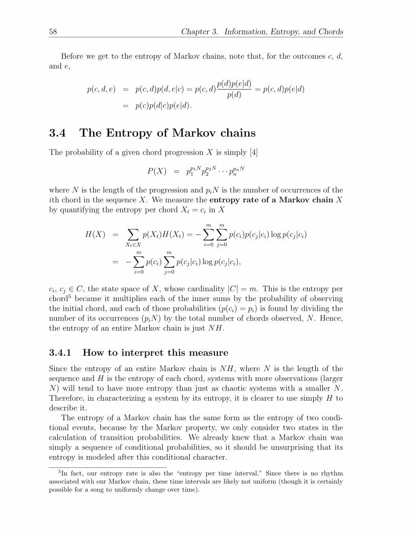
58 Chapter 3. Information, Entropy, and Chords
Before we get to the entropy of Markov chains, note that, for the outcomes c, d,and e,
p(c, d, e) = p(c, d)p(d, e|c) = p(c, d)p(d)p(e|d)
p(d)= p(c, d)p(e|d)
= p(c)p(d|c)p(e|d).
3.4 The Entropy of Markov chains
The probability of a given chord progression X is simply [4]
P (X) = pp1N1 pp2N2 · · · ppnNn
where N is the length of the progression and piN is the number of occurrences of theith chord in the sequence X. We measure the entropy rate of a Markov chain Xby quantifying the entropy per chord Xt = ci in X
H(X) =∑Xt∈X
p(Xt)H(Xt) = −m∑i=0
m∑j=0
p(ci)p(cj|ci) log p(cj|ci)
= −m∑i=0
p(ci)m∑j=0
p(cj|ci) log p(cj|ci),
ci, cj ∈ C, the state space of X, whose cardinality |C| = m. This is the entropy perchord5 because it multiplies each of the inner sums by the probability of observingthe initial chord, and each of those probabilities (p(ci) = pi) is found by dividing thenumber of its occurrences (piN) by the total number of chords observed, N . Hence,the entropy of an entire Markov chain is just NH.
3.4.1 How to interpret this measure
Since the entropy of an entire Markov chain is NH, where N is the length of thesequence and H is the entropy of each chord, systems with more observations (largerN) will tend to have more entropy than just as chaotic systems with a smaller N .Therefore, in characterizing a system by its entropy, it is clearer to use simply H todescribe it.
The entropy of a Markov chain has the same form as the entropy of two condi-tional events, because by the Markov property, we only consider two states in thecalculation of transition probabilities. We already knew that a Markov chain wassimply a sequence of conditional probabilities, so it should be unsurprising that itsentropy is modeled after this conditional character.
5In fact, our entropy rate is also the “entropy per time interval.” Since there is no rhythmassociated with our Markov chain, these time intervals are likely not uniform (though it is certainlypossible for a song to uniformly change over time).
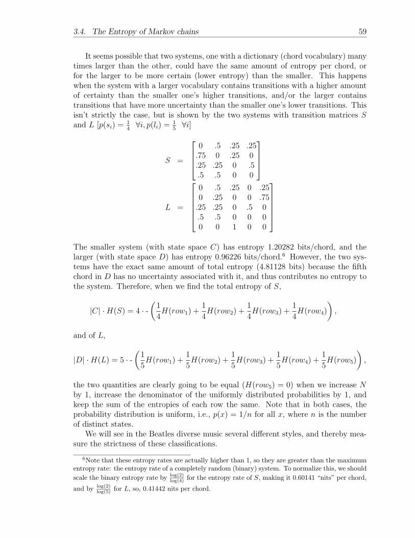
3.4. The Entropy of Markov chains 59
It seems possible that two systems, one with a dictionary (chord vocabulary) manytimes larger than the other, could have the same amount of entropy per chord, orfor the larger to be more certain (lower entropy) than the smaller. This happenswhen the system with a larger vocabulary contains transitions with a higher amountof certainty than the smaller one’s higher transitions, and/or the larger containstransitions that have more uncertainty than the smaller one’s lower transitions. Thisisn’t strictly the case, but is shown by the two systems with transition matrices Sand L [p(si) = 1
4∀i, p(li) = 1
5∀i]
S =
0 .5 .25 .25.75 0 .25 0.25 .25 0 .5.5 .5 0 0
L =
0 .5 .25 0 .250 .25 0 0 .75.25 .25 0 .5 0.5 .5 0 0 00 0 1 0 0
The smaller system (with state space C) has entropy 1.20282 bits/chord, and thelarger (with state space D) has entropy 0.96226 bits/chord.6 However, the two sys-tems have the exact same amount of total entropy (4.81128 bits) because the fifthchord in D has no uncertainty associated with it, and thus contributes no entropy tothe system. Therefore, when we find the total entropy of S,
|C| ·H(S) = 4 · -(
1
4H(row1) +
1
4H(row2) +
1
4H(row3) +
1
4H(row4)
),
and of L,
|D| ·H(L) = 5 · -(
1
5H(row1) +
1
5H(row2) +
1
5H(row3) +
1
5H(row4) +
1
5H(row5)
),
the two quantities are clearly going to be equal (H(row5) = 0) when we increase Nby 1, increase the denominator of the uniformly distributed probabilities by 1, andkeep the sum of the entropies of each row the same. Note that in both cases, theprobability distribution is uniform, i.e., p(x) = 1/n for all x, where n is the numberof distinct states.
We will see in the Beatles diverse music several different styles, and thereby mea-sure the strictness of these classifications.
6Note that these entropy rates are actually higher than 1, so they are greater than the maximumentropy rate: the entropy rate of a completely random (binary) system. To normalize this, we shouldscale the binary entropy rate by log(2)
log(4) for the entropy rate of S, making it 0.60141 “nits” per chord,
and by log(2)log(5) for L, so, 0.41442 nits per chord.
60 Chapter 3. Information, Entropy, and Chords
3.5 Expectations
Studying the entropy rate of a sequence of symbols is one way of determining theirunique source. For example, entropy has been applied to the four gospels of the Bibleto establish whether or not they were indeed written by four different authors—and itwas found that they were not!7 Music and art seem to borrow from previous materialmore shamelessly than literature, and artists can have a repertoire containing a vastrange of styles and instrumentation, whereas authors are usually confined to onelanguage, and cannot adapt their style so easily as a band of four or more musicianscan in parallel. Even when the members of a band do not collectively write theirsongs, each of their individual styles and preferences in instrumentation do appearin the frequency spectrum. Therefore, I suspect that the application of entropy tomusic will not specify artist, but rather, origin of the style.
As one listens to more and more music under distinct classifications, one startsto learn its language This is true especially of music that gains popularity, primarilybecause it is easy to discover. “What makes a hit?” is the big question amongstsongwriters—either because they want the satisfaction that goes with creating some-thing that has appeal and makes money, or because they want to discern what it isabout certain songs that appeals to them, and what turns them off. With a proba-bilistic model like a Markov chain, our quantified findings cannot be completely offbase with describing the tendencies of a set of music.
This is only because we name chords relative to their key, I would like to pointout. From the light spectrum, say that we treated “colors” like the scales of the key,[R, O, Y, G, B, I, V] = [1, 2, 3, 4, 5, 6, 7]. Do humans perceive the combination oforange (2) and violet (7) the same way they do red (1) and indigo (6)? Not in theway that humans cannot distinguish the root of sonic intervals, though interestingly,those of us that do have perfect pitch usually perceive distinct pitches as a uniquecolor in the spectrum!
But, maybe we should challenge the notion that perfect pitch (the ability to de-tect pitch, not limited to those on the keyboard) is a gift received at birth. Allegedly,the percent of humans with perfect pitch is something like 0.001%, and I’ve met justone in my lifetime (who did in fact have the color-pitch synesthesia). After this thesis,I can tell that I am much better at estimating pitch than before, though because Ising, I know almost the exact range that my voice can handle. The acquisition ofrelative pitch (the ability to detect melodic intervals) from years of music theory,plus knowing one’s vocal range, gives me all the tools I need to identify a note witha smaller amount of error.
Now, I expect popular music to have a noticeably lower entropy rate than anyother style, and popular musicians alike, just because popular songs are simple andpredictable on average. The Beatles were certainly interesting, but what gave themthat extra spark was their fun rhythms and lyrics, not necessarily complex chordprogressions. However, I would say that few other musicians used the same sets ofchords and transitions between chords that the Beatles did in their songs. Since I
7R. Crandall, private communication (2009).
3.5. Expectations 61
have played Beethoven and music from other classical musicians (though, I seem tohave a propensity for the Romantics), as well as some knowledge of music theory injazz, I know that many accidentals are used in the two styles. Therefore, I expect ahigher amount of entropy in these systems as well as a greater state space of chords.I do not expect the data from our bandpass filter to be noise-free, because I couldnot familiarize myself enough with the discrete Fourier transform to the point thatI could trust the frequencies it picks out to be fundamental frequencies, and not aharmonic thereof.
The Beatles released 11 studio albums (EP’s) to the U.K. in the following order8:
1963 : Please Please Me
1963 : With the Beatles
1964 : A Hard Day’s Night
1964 : Beatles for Sale
1965 : Help!
1965 : Rubber Soul
1966 : Revolver
1967 : Sgt. Pepper’s Lonely Hearts Club Band
1967 : The Magical Mystery Tour
1968 : The Beatles (White Album)
1969 : Yellow Submarine
1969 : Abbey Road
1969 : Let It Be
All of the albums feature fairly “unexpected” chords and chord progressions, butthe first few (before Rubber Soul, or arguably pre-Help! ) contain many songs thatsound remarkably alike, some of which are (highly predictable) standards not writtenby The Beatles. Then, in the albums Rubber Soul through Abbey Road, The Beatlesexpanded their musical vocabulary, or at least differentiated between songs on thesame album more. But their final album, Let It Be, they seemed to return to their oldsound. Because of this, comparing the affectation of a few of these albums should bea good test of our hypothesis that music under a loose classification, like “jazz,” has amore uniform Markov chain (or, it will be more like throwing a die), and music undera strict classification has a greater certainty about it. Below are a few songs withtheir chord names and, beneath those, the Roman numerical equivalent, to show youjust how their harmonic vocabulary grew—and with Let It Be, down-sized. I predict
8I have ordered this list as best I can, for the following anachronisms and peculiarities are true:(1) The Beatles released The Magical Mystery Tour to the U.K. in 1976 but to the U.S. upon itscompletion in 1967; (2) Yellow Submarine features many orchestral songs from the film of whichit is a soundtrack, but “Only a Northern Song,” “It’s All too Much,” “Hey Bulldog,” and “AllTogether Now” do not appear on any other album; and finally, (3) Abbey Road was actually the lastalbum The Beatles recorded but was released before Let It Be because of issues with Phil Spector’sdirection.
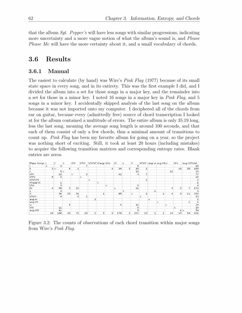
62 Chapter 3. Information, Entropy, and Chords
that the album Sgt. Pepper’s will have less songs with similar progressions, indicatingmore uncertainty and a more vague notion of what the album’s sound is, and PleasePlease Me will have the more certainty about it, and a small vocabulary of chords.
3.6 Results
3.6.1 Manual
The easiest to calculate (by hand) was Wire’s Pink Flag (1977) because of its smallstate space in every song, and in its entirety. This was the first example I did, and Idivided the album into a set for those songs in a major key, and the remainder intoa set for those in a minor key. I noted 16 songs in a major key in Pink Flag, and 5songs in a minor key. I accidentally skipped analysis of the last song on the albumbecause it was not imported onto my computer. I deciphered all of the chords fromear on guitar, because every (admittedly free) source of chord transcription I lookedat for the album contained a multitude of errors. The entire album is only 35:19 long,less the last song, meaning the average song length is around 100 seconds, and thateach of them consist of only a few chords, thus a minimal amount of transitions tocount up. Pink Flag has been my favorite album for going on a year, so the projectwas nothing short of exciting. Still, it took at least 20 hours (including mistakes)to acquire the following transition matrices and corresponding entropy rates. Blankentries are zeros.
Figure 3.2: The counts of observations of each chord transition within major songsfrom Wire’s Pink Flag.
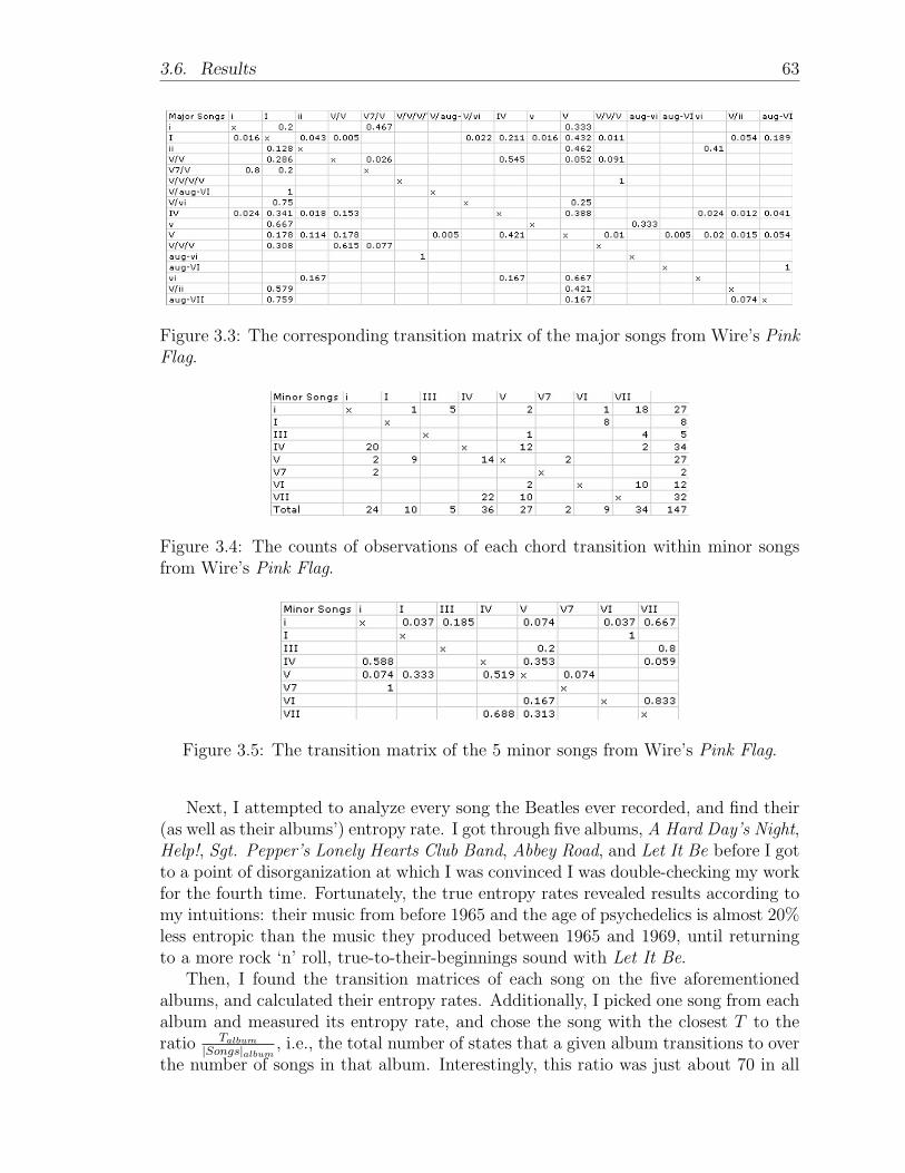
3.6. Results 63
Figure 3.3: The corresponding transition matrix of the major songs from Wire’s PinkFlag.
Figure 3.4: The counts of observations of each chord transition within minor songsfrom Wire’s Pink Flag.
Figure 3.5: The transition matrix of the 5 minor songs from Wire’s Pink Flag.
Next, I attempted to analyze every song the Beatles ever recorded, and find their(as well as their albums’) entropy rate. I got through five albums, A Hard Day’s Night,Help!, Sgt. Pepper’s Lonely Hearts Club Band, Abbey Road, and Let It Be before I gotto a point of disorganization at which I was convinced I was double-checking my workfor the fourth time. Fortunately, the true entropy rates revealed results according tomy intuitions: their music from before 1965 and the age of psychedelics is almost 20%less entropic than the music they produced between 1965 and 1969, until returningto a more rock ‘n’ roll, true-to-their-beginnings sound with Let It Be.
Then, I found the transition matrices of each song on the five aforementionedalbums, and calculated their entropy rates. Additionally, I picked one song from eachalbum and measured its entropy rate, and chose the song with the closest T to theratio Talbum
|Songs|album, i.e., the total number of states that a given album transitions to over
the number of songs in that album. Interestingly, this ratio was just about 70 in all
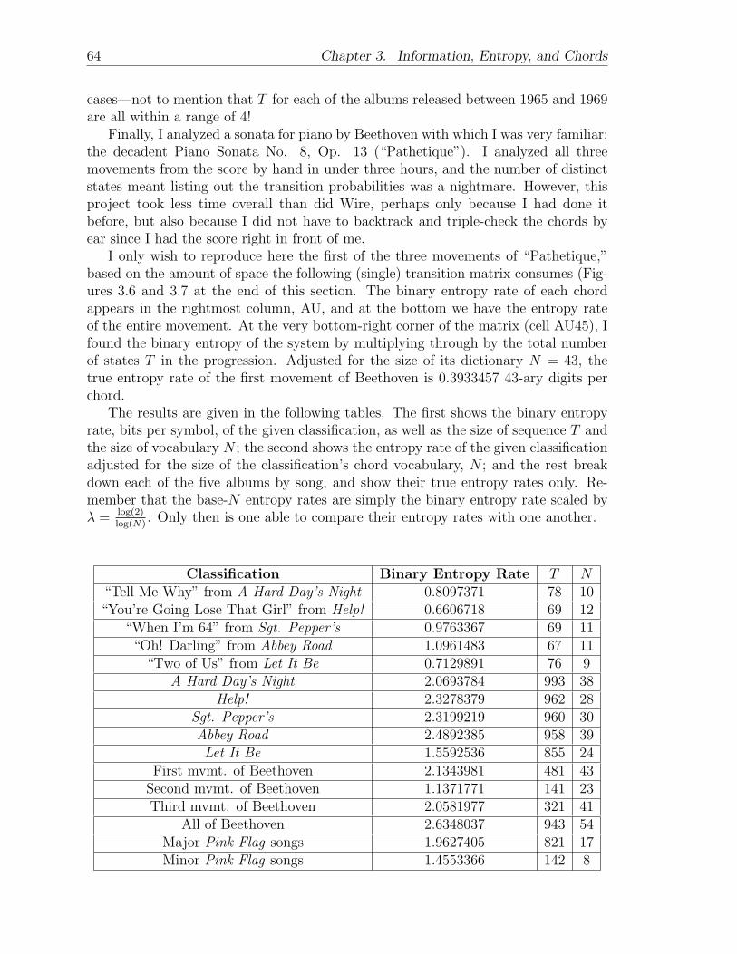
64 Chapter 3. Information, Entropy, and Chords
cases—not to mention that T for each of the albums released between 1965 and 1969are all within a range of 4!
Finally, I analyzed a sonata for piano by Beethoven with which I was very familiar:the decadent Piano Sonata No. 8, Op. 13 (“Pathetique”). I analyzed all threemovements from the score by hand in under three hours, and the number of distinctstates meant listing out the transition probabilities was a nightmare. However, thisproject took less time overall than did Wire, perhaps only because I had done itbefore, but also because I did not have to backtrack and triple-check the chords byear since I had the score right in front of me.
I only wish to reproduce here the first of the three movements of “Pathetique,”based on the amount of space the following (single) transition matrix consumes (Fig-ures 3.6 and 3.7 at the end of this section. The binary entropy rate of each chordappears in the rightmost column, AU, and at the bottom we have the entropy rateof the entire movement. At the very bottom-right corner of the matrix (cell AU45), Ifound the binary entropy of the system by multiplying through by the total numberof states T in the progression. Adjusted for the size of its dictionary N = 43, thetrue entropy rate of the first movement of Beethoven is 0.3933457 43-ary digits perchord.
The results are given in the following tables. The first shows the binary entropyrate, bits per symbol, of the given classification, as well as the size of sequence T andthe size of vocabulary N ; the second shows the entropy rate of the given classificationadjusted for the size of the classification’s chord vocabulary, N ; and the rest breakdown each of the five albums by song, and show their true entropy rates only. Re-member that the base-N entropy rates are simply the binary entropy rate scaled byλ = log(2)
log(N). Only then is one able to compare their entropy rates with one another.
Classification Binary Entropy Rate T N“Tell Me Why” from A Hard Day’s Night 0.8097371 78 10“You’re Going Lose That Girl” from Help! 0.6606718 69 12
“When I’m 64” from Sgt. Pepper’s 0.9763367 69 11“Oh! Darling” from Abbey Road 1.0961483 67 11
“Two of Us” from Let It Be 0.7129891 76 9A Hard Day’s Night 2.0693784 993 38
Help! 2.3278379 962 28Sgt. Pepper’s 2.3199219 960 30Abbey Road 2.4892385 958 39
Let It Be 1.5592536 855 24First mvmt. of Beethoven 2.1343981 481 43
Second mvmt. of Beethoven 1.1371771 141 23Third mvmt. of Beethoven 2.0581977 321 41
All of Beethoven 2.6348037 943 54Major Pink Flag songs 1.9627405 821 17Minor Pink Flag songs 1.4553366 142 8
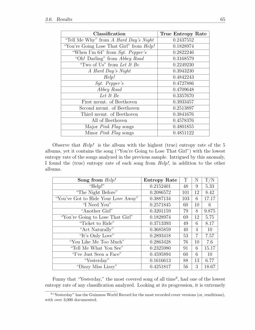
3.6. Results 65
Classification True Entropy Rate“Tell Me Why” from A Hard Day’s Night 0.2437552“You’re Going Lose That Girl” from Help! 0.1828974
“When I’m 64” from Sgt. Pepper’s 0.2822246“Oh! Darling” from Abbey Road 0.3168579
“Two of Us” from Let It Be 0.2249230A Hard Day’s Night 0.3943230
Help! 0.4842243Sgt. Pepper’s 0.4727886Abbey Road 0.4709648
Let It Be 0.3357670First mvmt. of Beethoven 0.3933457
Second mvmt. of Beethoven 0.2513897Third mvmt. of Beethoven 0.3841676
All of Beethoven 0.4578376Major Pink Flag songs 0.4801855Minor Pink Flag songs 0.4851122
Observe that Help! is the album with the highest (true) entropy rate of the 5albums, yet it contains the song (“You’re Going to Lose That Girl”) with the lowestentropy rate of the songs analyzed in the previous sample. Intrigued by this anomaly,I found the (true) entropy rate of each song from Help!, in addition to the otheralbums.
Song from Help! Entropy Rate T N T/N“Help!” 0.2152401 48 9 5.33
“The Night Before” 0.2086572 101 12 8.42“You’ve Got to Hide Your Love Away” 0.3887134 103 6 17.17
“I Need You” 0.2571845 60 10 6“Another Girl” 0.3201159 79 8 9.875
“You’re Going to Lose That Girl” 0.1828974 69 12 5.75“Ticket to Ride” 0.3713393 49 6 8.17“Act Naturally” 0.3685859 40 4 10“It’s Only Love” 0.2893418 53 7 7.57
“You Like Me Too Much” 0.2863428 76 10 7.6“Tell Me What You See” 0.2325980 91 6 15.17“I’ve Just Seen a Face” 0.4595894 60 6 10
“Yesterday” 0.1616613 88 13 6.77“Dizzy Miss Lizzy” 0.4251817 56 3 18.67
Funny that “Yesterday,” the most covered song of all time9, had one of the lowestentropy rate of any classification analyzed. Looking at its progression, it is extremely
9“Yesterday” has the Guinness World Record for the most recorded cover versions (or, renditions),with over 3,000 documented.
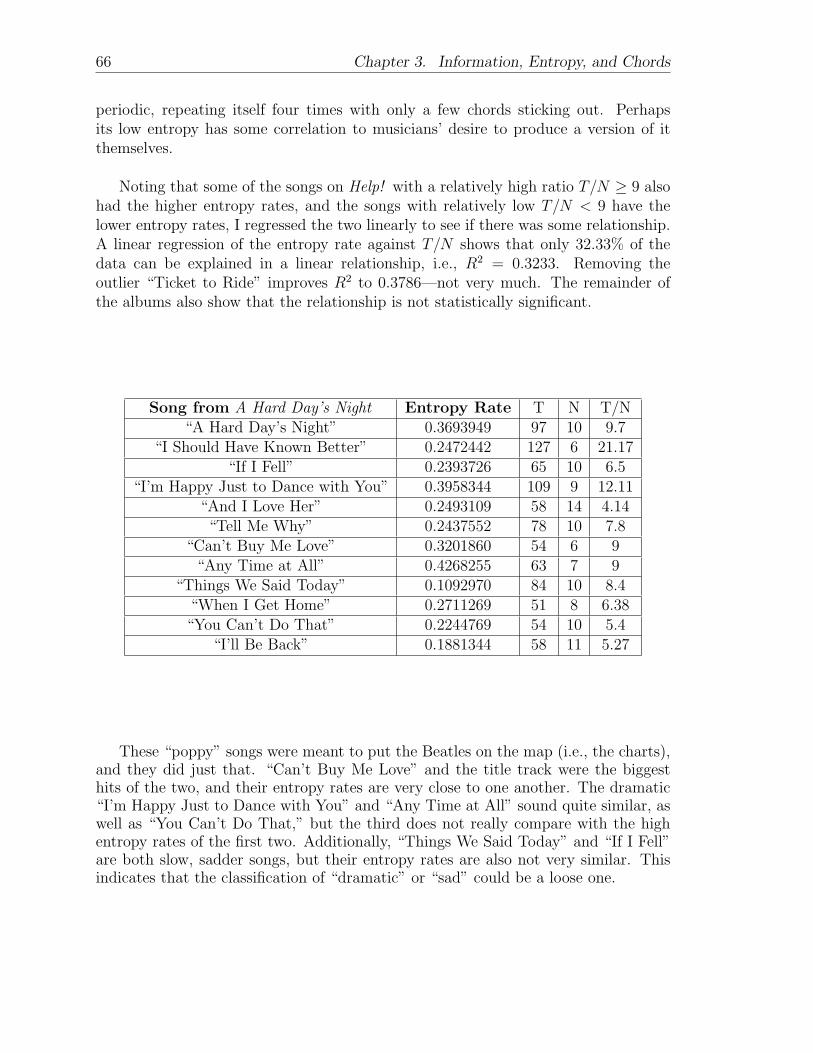
66 Chapter 3. Information, Entropy, and Chords
periodic, repeating itself four times with only a few chords sticking out. Perhapsits low entropy has some correlation to musicians’ desire to produce a version of itthemselves.
Noting that some of the songs on Help! with a relatively high ratio T/N ≥ 9 alsohad the higher entropy rates, and the songs with relatively low T/N < 9 have thelower entropy rates, I regressed the two linearly to see if there was some relationship.A linear regression of the entropy rate against T/N shows that only 32.33% of thedata can be explained in a linear relationship, i.e., R2 = 0.3233. Removing theoutlier “Ticket to Ride” improves R2 to 0.3786—not very much. The remainder ofthe albums also show that the relationship is not statistically significant.
Song from A Hard Day’s Night Entropy Rate T N T/N“A Hard Day’s Night” 0.3693949 97 10 9.7
“I Should Have Known Better” 0.2472442 127 6 21.17“If I Fell” 0.2393726 65 10 6.5
“I’m Happy Just to Dance with You” 0.3958344 109 9 12.11“And I Love Her” 0.2493109 58 14 4.14“Tell Me Why” 0.2437552 78 10 7.8
“Can’t Buy Me Love” 0.3201860 54 6 9“Any Time at All” 0.4268255 63 7 9
“Things We Said Today” 0.1092970 84 10 8.4“When I Get Home” 0.2711269 51 8 6.38“You Can’t Do That” 0.2244769 54 10 5.4
“I’ll Be Back” 0.1881344 58 11 5.27
These “poppy” songs were meant to put the Beatles on the map (i.e., the charts),and they did just that. “Can’t Buy Me Love” and the title track were the biggesthits of the two, and their entropy rates are very close to one another. The dramatic“I’m Happy Just to Dance with You” and “Any Time at All” sound quite similar, aswell as “You Can’t Do That,” but the third does not really compare with the highentropy rates of the first two. Additionally, “Things We Said Today” and “If I Fell”are both slow, sadder songs, but their entropy rates are also not very similar. Thisindicates that the classification of “dramatic” or “sad” could be a loose one.
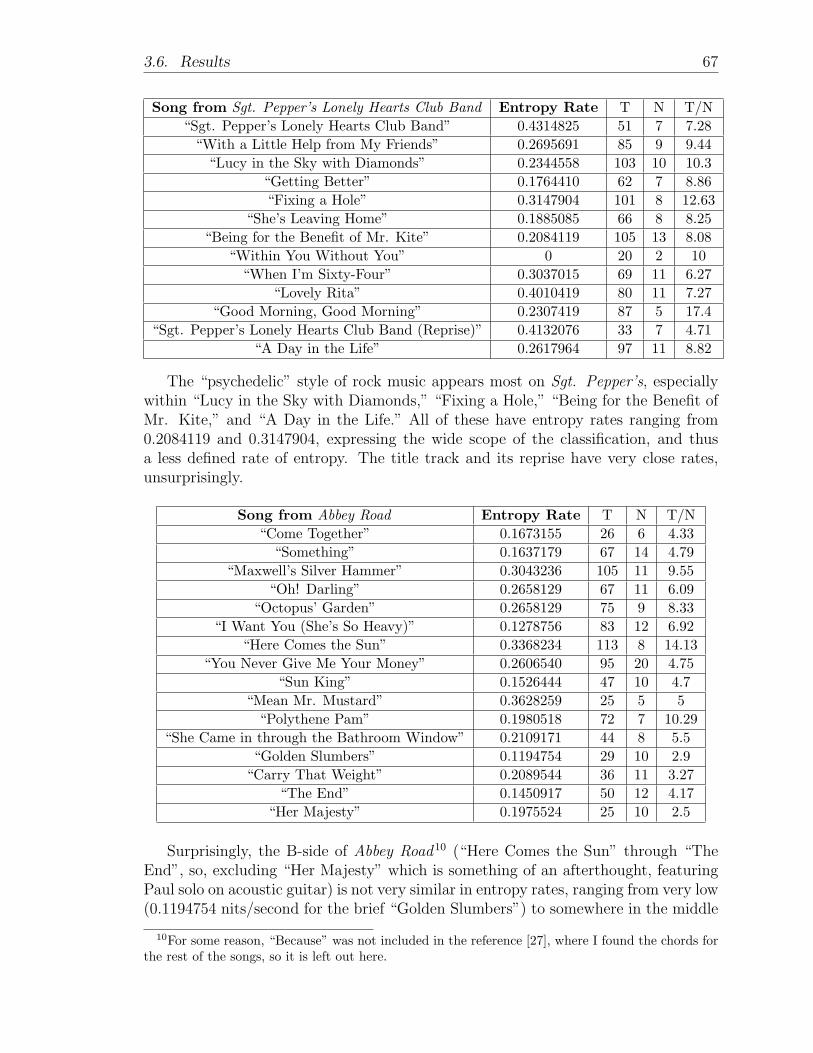
3.6. Results 67
Song from Sgt. Pepper’s Lonely Hearts Club Band Entropy Rate T N T/N“Sgt. Pepper’s Lonely Hearts Club Band” 0.4314825 51 7 7.28
“With a Little Help from My Friends” 0.2695691 85 9 9.44“Lucy in the Sky with Diamonds” 0.2344558 103 10 10.3
“Getting Better” 0.1764410 62 7 8.86“Fixing a Hole” 0.3147904 101 8 12.63
“She’s Leaving Home” 0.1885085 66 8 8.25“Being for the Benefit of Mr. Kite” 0.2084119 105 13 8.08
“Within You Without You” 0 20 2 10“When I’m Sixty-Four” 0.3037015 69 11 6.27
“Lovely Rita” 0.4010419 80 11 7.27“Good Morning, Good Morning” 0.2307419 87 5 17.4
“Sgt. Pepper’s Lonely Hearts Club Band (Reprise)” 0.4132076 33 7 4.71“A Day in the Life” 0.2617964 97 11 8.82
The “psychedelic” style of rock music appears most on Sgt. Pepper’s, especiallywithin “Lucy in the Sky with Diamonds,” “Fixing a Hole,” “Being for the Benefit ofMr. Kite,” and “A Day in the Life.” All of these have entropy rates ranging from0.2084119 and 0.3147904, expressing the wide scope of the classification, and thusa less defined rate of entropy. The title track and its reprise have very close rates,unsurprisingly.
Song from Abbey Road Entropy Rate T N T/N“Come Together” 0.1673155 26 6 4.33
“Something” 0.1637179 67 14 4.79“Maxwell’s Silver Hammer” 0.3043236 105 11 9.55
“Oh! Darling” 0.2658129 67 11 6.09“Octopus’ Garden” 0.2658129 75 9 8.33
“I Want You (She’s So Heavy)” 0.1278756 83 12 6.92“Here Comes the Sun” 0.3368234 113 8 14.13
“You Never Give Me Your Money” 0.2606540 95 20 4.75“Sun King” 0.1526444 47 10 4.7
“Mean Mr. Mustard” 0.3628259 25 5 5“Polythene Pam” 0.1980518 72 7 10.29
“She Came in through the Bathroom Window” 0.2109171 44 8 5.5“Golden Slumbers” 0.1194754 29 10 2.9
“Carry That Weight” 0.2089544 36 11 3.27“The End” 0.1450917 50 12 4.17
“Her Majesty” 0.1975524 25 10 2.5
Surprisingly, the B-side of Abbey Road10 (“Here Comes the Sun” through “TheEnd”, so, excluding “Her Majesty” which is something of an afterthought, featuringPaul solo on acoustic guitar) is not very similar in entropy rates, ranging from very low(0.1194754 nits/second for the brief “Golden Slumbers”) to somewhere in the middle
10For some reason, “Because” was not included in the reference [27], where I found the chords forthe rest of the songs, so it is left out here.
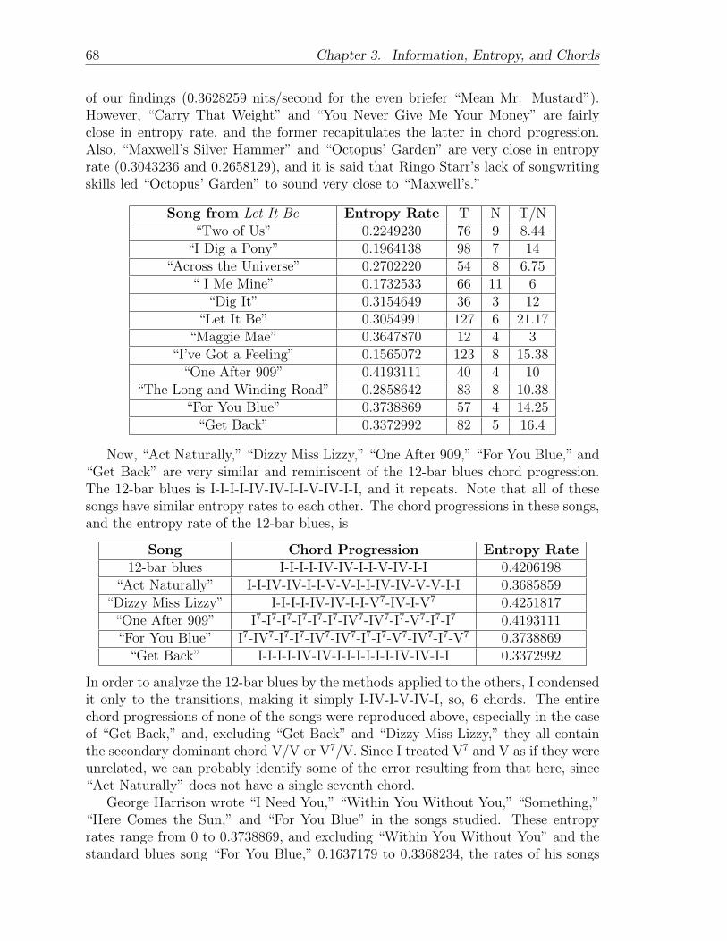
68 Chapter 3. Information, Entropy, and Chords
of our findings (0.3628259 nits/second for the even briefer “Mean Mr. Mustard”).However, “Carry That Weight” and “You Never Give Me Your Money” are fairlyclose in entropy rate, and the former recapitulates the latter in chord progression.Also, “Maxwell’s Silver Hammer” and “Octopus’ Garden” are very close in entropyrate (0.3043236 and 0.2658129), and it is said that Ringo Starr’s lack of songwritingskills led “Octopus’ Garden” to sound very close to “Maxwell’s.”
Song from Let It Be Entropy Rate T N T/N“Two of Us” 0.2249230 76 9 8.44
“I Dig a Pony” 0.1964138 98 7 14“Across the Universe” 0.2702220 54 8 6.75
“ I Me Mine” 0.1732533 66 11 6“Dig It” 0.3154649 36 3 12
“Let It Be” 0.3054991 127 6 21.17“Maggie Mae” 0.3647870 12 4 3
“I’ve Got a Feeling” 0.1565072 123 8 15.38“One After 909” 0.4193111 40 4 10
“The Long and Winding Road” 0.2858642 83 8 10.38“For You Blue” 0.3738869 57 4 14.25
“Get Back” 0.3372992 82 5 16.4
Now, “Act Naturally,” “Dizzy Miss Lizzy,” “One After 909,” “For You Blue,” and“Get Back” are very similar and reminiscent of the 12-bar blues chord progression.The 12-bar blues is I-I-I-I-IV-IV-I-I-V-IV-I-I, and it repeats. Note that all of thesesongs have similar entropy rates to each other. The chord progressions in these songs,and the entropy rate of the 12-bar blues, is
Song Chord Progression Entropy Rate12-bar blues I-I-I-I-IV-IV-I-I-V-IV-I-I 0.4206198
“Act Naturally” I-I-IV-IV-I-I-V-V-I-I-IV-IV-V-V-I-I 0.3685859“Dizzy Miss Lizzy” I-I-I-I-IV-IV-I-I-V7-IV-I-V7 0.4251817
“One After 909” I7-I7-I7-I7-I7-I7-IV7-IV7-I7-V7-I7-I7 0.4193111“For You Blue” I7-IV7-I7-I7-IV7-IV7-I7-I7-V7-IV7-I7-V7 0.3738869
“Get Back” I-I-I-I-IV-IV-I-I-I-I-I-I-IV-IV-I-I 0.3372992
In order to analyze the 12-bar blues by the methods applied to the others, I condensedit only to the transitions, making it simply I-IV-I-V-IV-I, so, 6 chords. The entirechord progressions of none of the songs were reproduced above, especially in the caseof “Get Back,” and, excluding “Get Back” and “Dizzy Miss Lizzy,” they all containthe secondary dominant chord V/V or V7/V. Since I treated V7 and V as if they wereunrelated, we can probably identify some of the error resulting from that here, since“Act Naturally” does not have a single seventh chord.
George Harrison wrote “I Need You,” “Within You Without You,” “Something,”“Here Comes the Sun,” and “For You Blue” in the songs studied. These entropyrates range from 0 to 0.3738869, and excluding “Within You Without You” and thestandard blues song “For You Blue,” 0.1637179 to 0.3368234, the rates of his songs
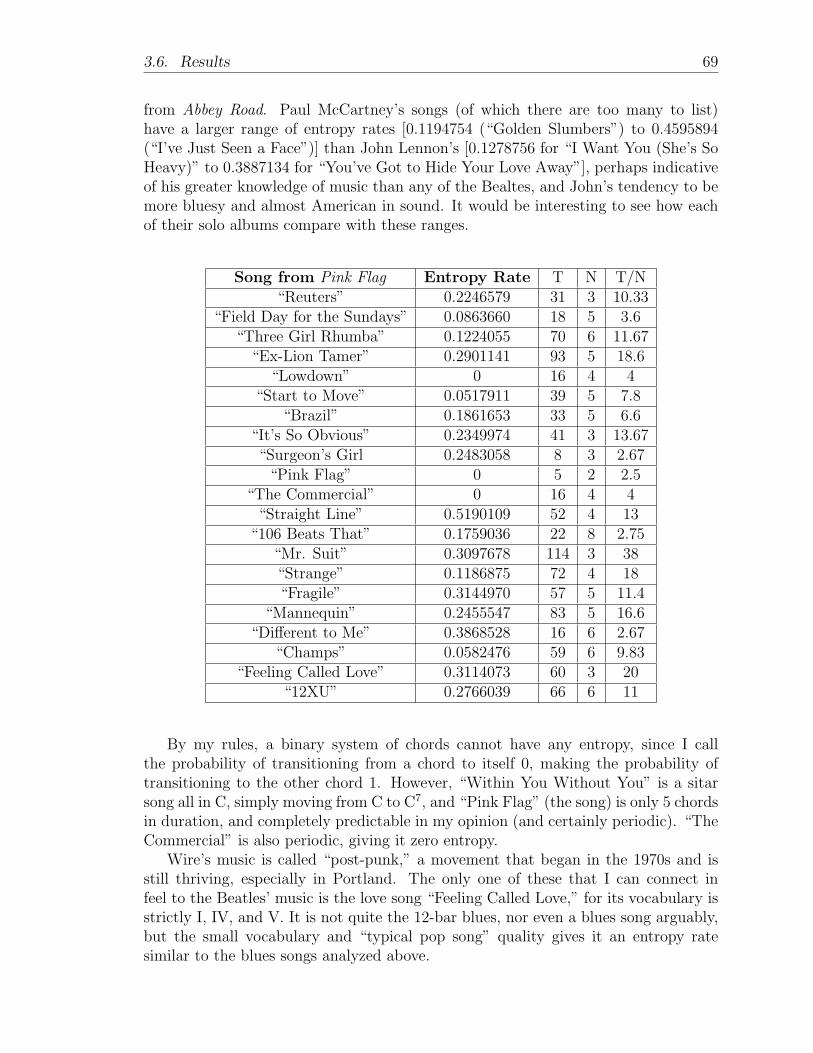
3.6. Results 69
from Abbey Road. Paul McCartney’s songs (of which there are too many to list)have a larger range of entropy rates [0.1194754 (“Golden Slumbers”) to 0.4595894(“I’ve Just Seen a Face”)] than John Lennon’s [0.1278756 for “I Want You (She’s SoHeavy)” to 0.3887134 for “You’ve Got to Hide Your Love Away”], perhaps indicativeof his greater knowledge of music than any of the Bealtes, and John’s tendency to bemore bluesy and almost American in sound. It would be interesting to see how eachof their solo albums compare with these ranges.
Song from Pink Flag Entropy Rate T N T/N“Reuters” 0.2246579 31 3 10.33
“Field Day for the Sundays” 0.0863660 18 5 3.6“Three Girl Rhumba” 0.1224055 70 6 11.67
“Ex-Lion Tamer” 0.2901141 93 5 18.6“Lowdown” 0 16 4 4
“Start to Move” 0.0517911 39 5 7.8“Brazil” 0.1861653 33 5 6.6
“It’s So Obvious” 0.2349974 41 3 13.67“Surgeon’s Girl 0.2483058 8 3 2.67
“Pink Flag” 0 5 2 2.5“The Commercial” 0 16 4 4
“Straight Line” 0.5190109 52 4 13“106 Beats That” 0.1759036 22 8 2.75
“Mr. Suit” 0.3097678 114 3 38“Strange” 0.1186875 72 4 18“Fragile” 0.3144970 57 5 11.4
“Mannequin” 0.2455547 83 5 16.6“Different to Me” 0.3868528 16 6 2.67
“Champs” 0.0582476 59 6 9.83“Feeling Called Love” 0.3114073 60 3 20
“12XU” 0.2766039 66 6 11
By my rules, a binary system of chords cannot have any entropy, since I callthe probability of transitioning from a chord to itself 0, making the probability oftransitioning to the other chord 1. However, “Within You Without You” is a sitarsong all in C, simply moving from C to C7, and “Pink Flag” (the song) is only 5 chordsin duration, and completely predictable in my opinion (and certainly periodic). “TheCommercial” is also periodic, giving it zero entropy.
Wire’s music is called “post-punk,” a movement that began in the 1970s and isstill thriving, especially in Portland. The only one of these that I can connect infeel to the Beatles’ music is the love song “Feeling Called Love,” for its vocabulary isstrictly I, IV, and V. It is not quite the 12-bar blues, nor even a blues song arguably,but the small vocabulary and “typical pop song” quality gives it an entropy ratesimilar to the blues songs analyzed above.
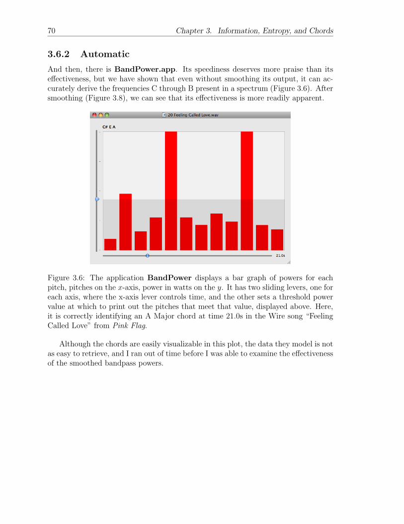
70 Chapter 3. Information, Entropy, and Chords
3.6.2 Automatic
And then, there is BandPower.app. Its speediness deserves more praise than itseffectiveness, but we have shown that even without smoothing its output, it can ac-curately derive the frequencies C through B present in a spectrum (Figure 3.6). Aftersmoothing (Figure 3.8), we can see that its effectiveness is more readily apparent.
Figure 3.6: The application BandPower displays a bar graph of powers for eachpitch, pitches on the x-axis, power in watts on the y. It has two sliding levers, one foreach axis, where the x-axis lever controls time, and the other sets a threshold powervalue at which to print out the pitches that meet that value, displayed above. Here,it is correctly identifying an A Major chord at time 21.0s in the Wire song “FeelingCalled Love” from Pink Flag.
Although the chords are easily visualizable in this plot, the data they model is notas easy to retrieve, and I ran out of time before I was able to examine the effectivenessof the smoothed bandpass powers.
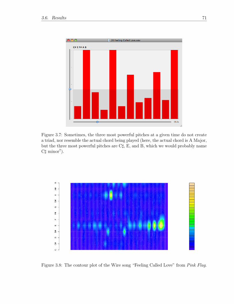
3.6. Results 71
Figure 3.7: Sometimes, the three most powerful pitches at a given time do not createa triad, nor resemble the actual chord being played (here, the actual chord is A Major,but the three most powerful pitches are C], E, and B, which we would probably nameC] minor7).
Figure 3.8: The contour plot of the Wire song “Feeling Called Love” from Pink Flag.
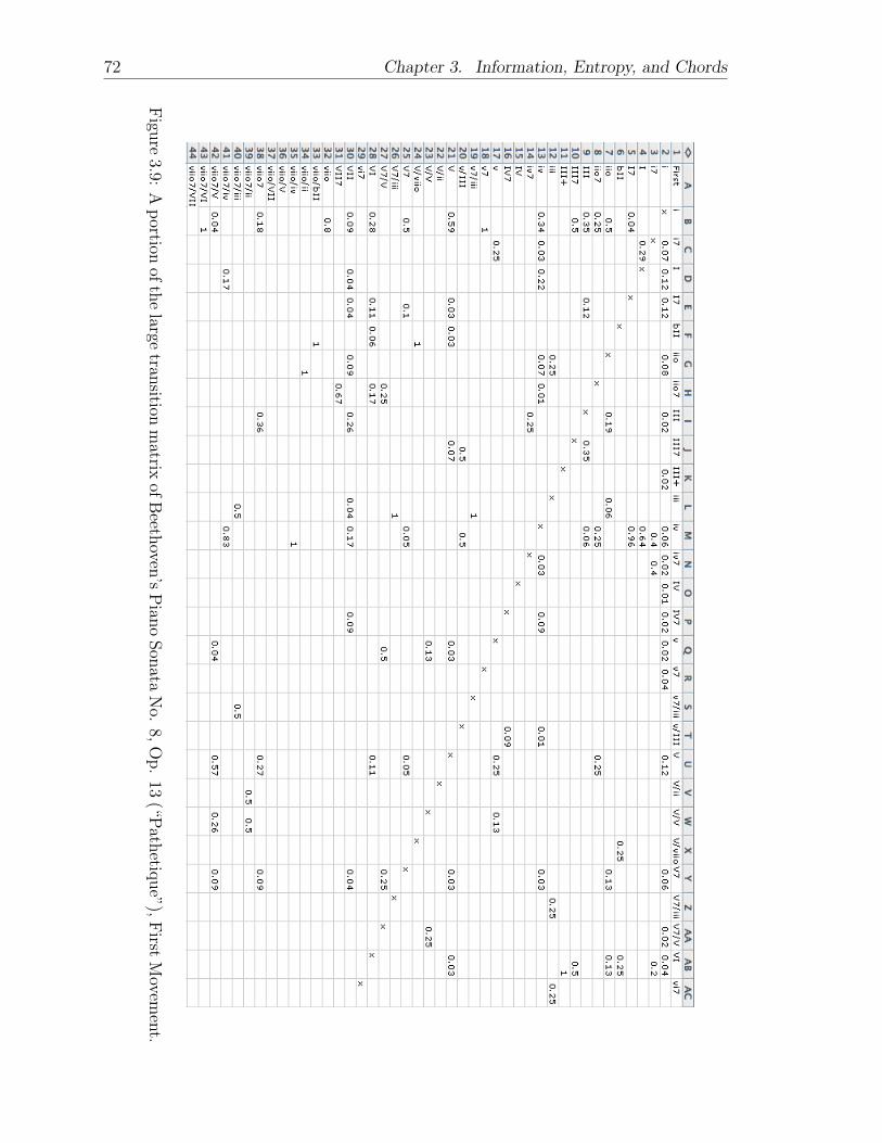
72 Chapter 3. Information, Entropy, and Chords
Figu
re3.9:
Ap
ortionof
the
largetran
sitionm
atrixof
Beeth
oven’s
Pian
oSon
ataN
o.8,
Op.
13(“P
athetiq
ue”),
First
Movem
ent.
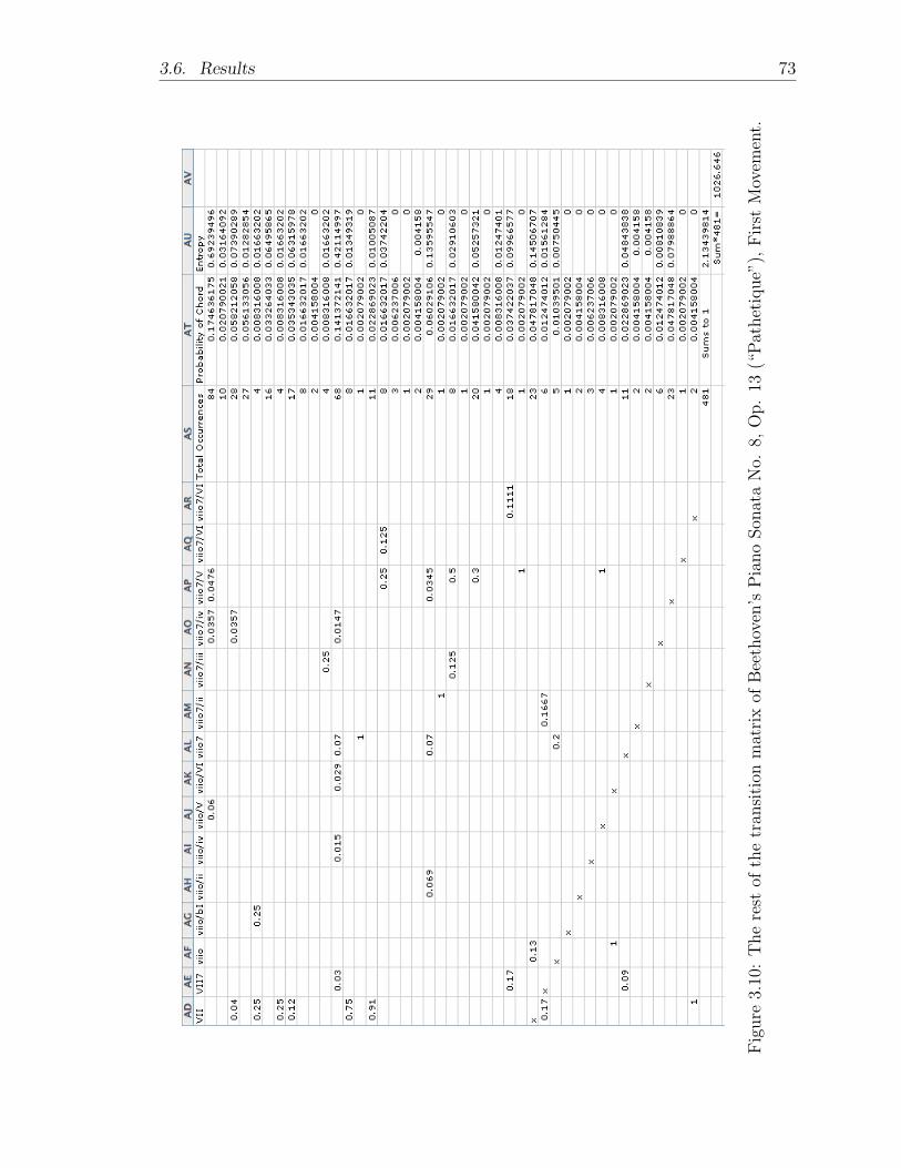
3.6. Results 73
Fig
ure
3.10
:T
he
rest
ofth
etr
ansi
tion
mat
rix
ofB
eeth
oven
’sP
iano
Son
ata
No.
8,O
p.
13(“
Pat
het
ique”
),F
irst
Mov
emen
t.

Conclusion
The application BandPower.app successfully picks out frequencies from the West-ern, 12-pitch scale, and allows one to view the frequencies excited at any time inthe scale, and set some threshold value for their amplitude in order to retrieve thefrequencies with the most power. By smoothing these results, we can throw out theunexplained (and not meaningful) pitches that often but irregularly appear, and keepthe ones that locally and consistently appear. The fact that BandPower.app runsin less than 10 seconds (for any WAVE-format file converted within iTunes) is a realachievement, and I anticipate even smarter versions of it to come.
The values of the calculated entropy rates from musical examples did not matchmy intuitions, in general—but they did show me that it isn’t the value, it is the rangeof values. Indeed, the blues songs studied had very similar entropy rates, and thepsychedelic and emotional ones had a wider range of them. It is hard to say thatthis is the case for the classification in general, of course, since our sample size wasso small, but is intriguing nonetheless.
If we did consider rhythm in our Markov chain, the entropy rates would mostcertainly turn out considerably different, and identify the true chaos of a classificationmuch more accurately. Consider, for example, the song “Tomorrow Never Knows” bythe Beatles, featuring just one chord: C Major. This song cannot be a Markov chainby my rules, because a row that sums to 0 in the transition matrix implies that thegiven state does not exist in C, the state space of the song. And, as mentioned before,songs with only 2 chords also have 0 entropy, since by my rules, the probability oftransitioning to the other chord is automatically 1.
Another method which I did not implement that would improve the ranges ofentropy rates toward my association of it with “strictness of musical classification”is the assignment of relative weights to those states that are closely related. Forinstance, the chords V, v, and V7 function harmonically more closely than do ii, VI,and viio, in general. Songs containing chords such that some of them have the sameroot should therefore be adjusted to have lower entropy than other songs with thesame amount of states but less of these “neighborhoods” of chords.
It is also possible that, generally speaking, music is not an ergodic, and thus not anaperiodic, Markov chain. Support for this claim comes from repetition of the sameprogressions for each verse, chorus, and bridge of virtually all popular songs—i.e.,there exist patterns governed by rhythm (and hence periodic) within chord progres-sions. It makes sense that, because we ignored rhythm, the T above is too small in allcases, since it documents only times when we move from the present chord. However,
76 Conclusion
if it were indeed not ergodic, this fact would not affect our calculated entropy rates.In summary, musicians should be less hesitant to apply mathematics to songwrit-
ing and the art of music, just as we have to language with linguistics. Those whosedevotion to music extends to seeking out the best training for their personal style,practicing for hours on end to perfect the fluidity of movement on their instrument(s),must be well acquainted with the probabilistic nature of their sound, whether theytreat it mathematically, or with a qualitative, psychological sense of likelihood. I un-derstand that boiling down music to probability theory is a little dry (and also insistthat I have hardly “boiled things down” here, as I analyzed only chord progressions inmusic, something liberated by expression), but what if it is the solution to the greatenigma that is our musical memory? It is no wonder that I applied many of the sametechniques used in speech recognition to music, for music is a language, and thosewho love to speak it have one of the richest and most accessible ways of escaping fromreality.
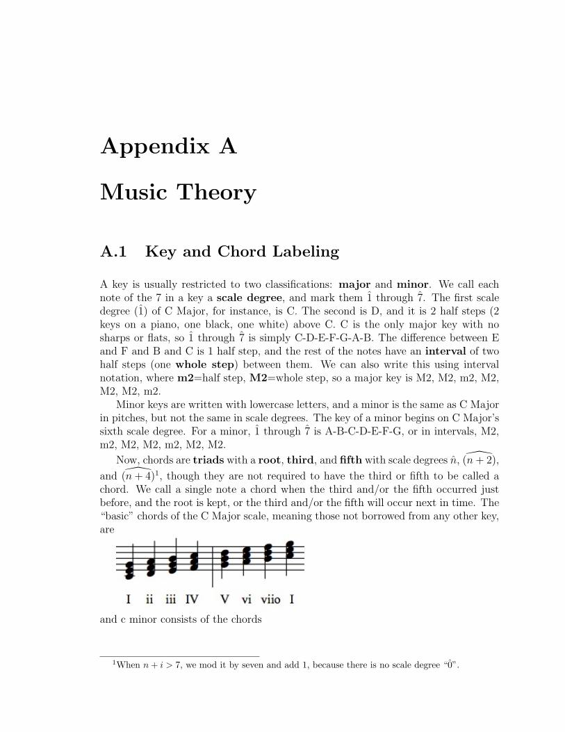
Appendix A
Music Theory
A.1 Key and Chord Labeling
A key is usually restricted to two classifications: major and minor. We call eachnote of the 7 in a key a scale degree, and mark them 1 through 7. The first scaledegree (1) of C Major, for instance, is C. The second is D, and it is 2 half steps (2keys on a piano, one black, one white) above C. C is the only major key with nosharps or flats, so 1 through 7 is simply C-D-E-F-G-A-B. The difference between Eand F and B and C is 1 half step, and the rest of the notes have an interval of twohalf steps (one whole step) between them. We can also write this using intervalnotation, where m2=half step, M2=whole step, so a major key is M2, M2, m2, M2,M2, M2, m2.
Minor keys are written with lowercase letters, and a minor is the same as C Majorin pitches, but not the same in scale degrees. The key of a minor begins on C Major’ssixth scale degree. For a minor, 1 through 7 is A-B-C-D-E-F-G, or in intervals, M2,m2, M2, M2, m2, M2, M2.
Now, chords are triads with a root, third, and fifth with scale degrees n, (n+ 2),
and (n+ 4)1, though they are not required to have the third or fifth to be called achord. We call a single note a chord when the third and/or the fifth occurred justbefore, and the root is kept, or the third and/or the fifth will occur next in time. The“basic” chords of the C Major scale, meaning those not borrowed from any other key,are
and c minor consists of the chords
1When n+ i > 7, we mod it by seven and add 1, because there is no scale degree “0”.
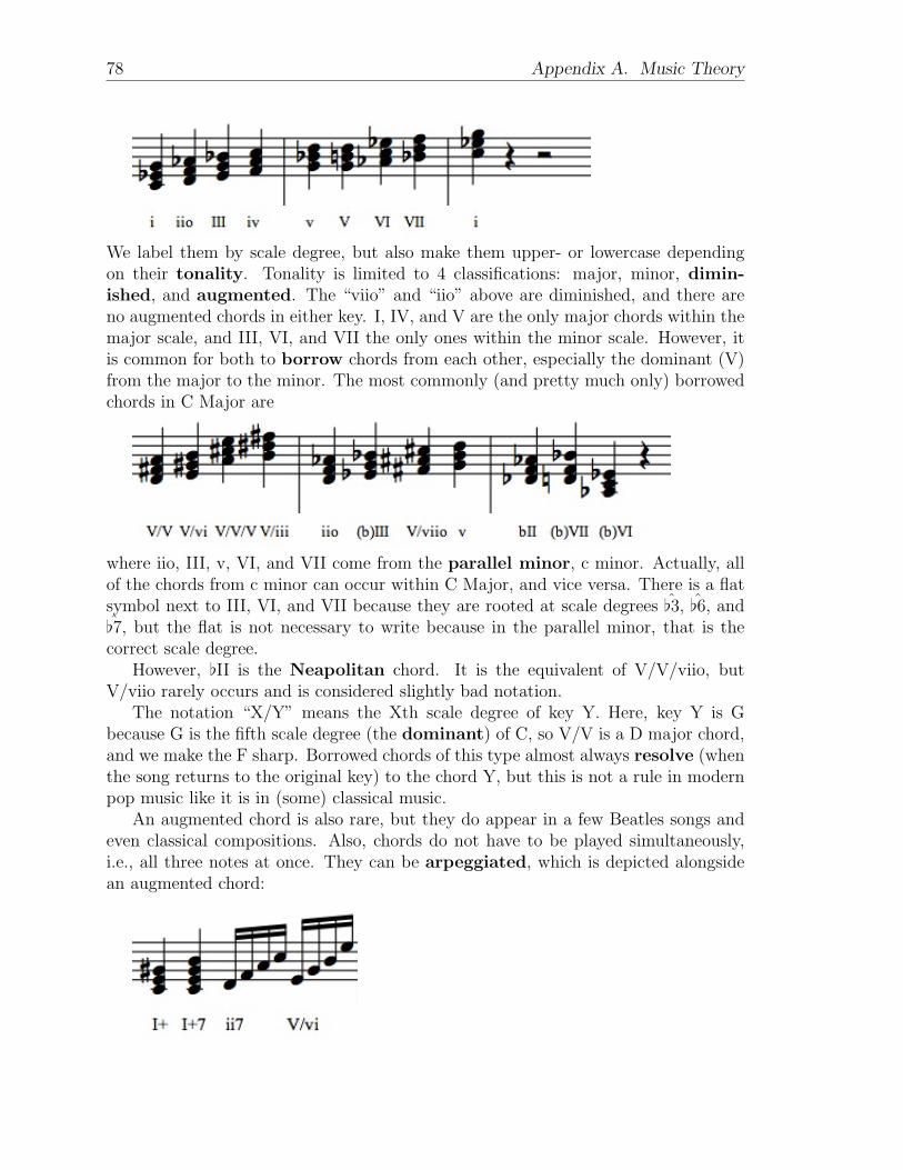
78 Appendix A. Music Theory
We label them by scale degree, but also make them upper- or lowercase dependingon their tonality. Tonality is limited to 4 classifications: major, minor, dimin-ished, and augmented. The “viio” and “iio” above are diminished, and there areno augmented chords in either key. I, IV, and V are the only major chords within themajor scale, and III, VI, and VII the only ones within the minor scale. However, itis common for both to borrow chords from each other, especially the dominant (V)from the major to the minor. The most commonly (and pretty much only) borrowedchords in C Major are
where iio, III, v, VI, and VII come from the parallel minor, c minor. Actually, allof the chords from c minor can occur within C Major, and vice versa. There is a flatsymbol next to III, VI, and VII because they are rooted at scale degrees [3, [6, and[7, but the flat is not necessary to write because in the parallel minor, that is thecorrect scale degree.
However, [II is the Neapolitan chord. It is the equivalent of V/V/viio, butV/viio rarely occurs and is considered slightly bad notation.
The notation “X/Y” means the Xth scale degree of key Y. Here, key Y is Gbecause G is the fifth scale degree (the dominant) of C, so V/V is a D major chord,and we make the F sharp. Borrowed chords of this type almost always resolve (whenthe song returns to the original key) to the chord Y, but this is not a rule in modernpop music like it is in (some) classical music.
An augmented chord is also rare, but they do appear in a few Beatles songs andeven classical compositions. Also, chords do not have to be played simultaneously,i.e., all three notes at once. They can be arpeggiated, which is depicted alongsidean augmented chord:
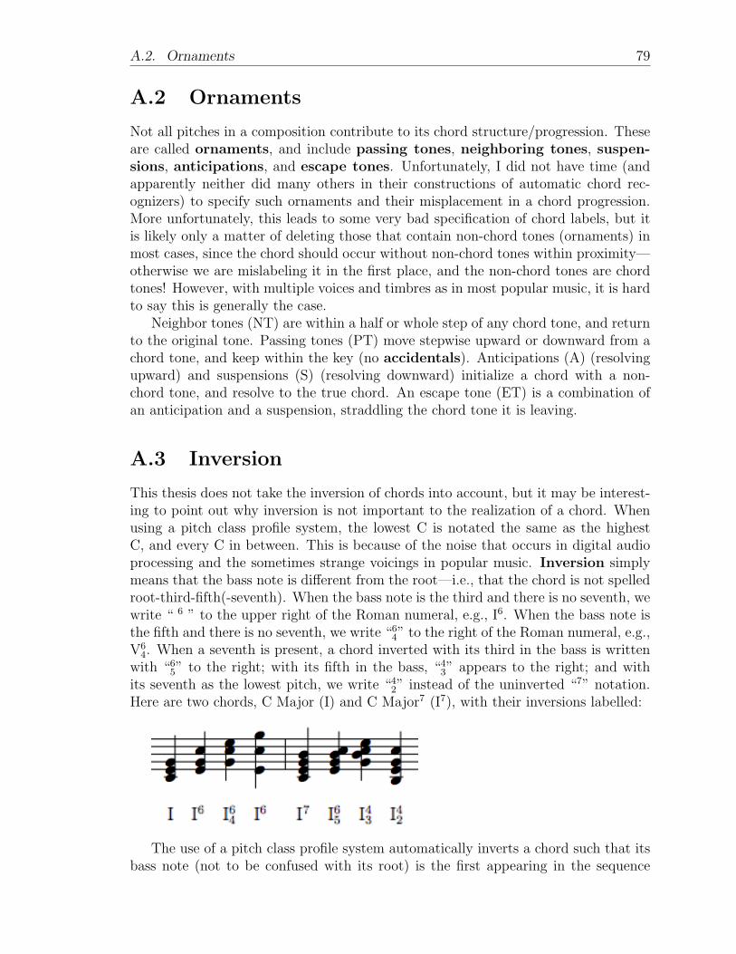
A.2. Ornaments 79
A.2 Ornaments
Not all pitches in a composition contribute to its chord structure/progression. Theseare called ornaments, and include passing tones, neighboring tones, suspen-sions, anticipations, and escape tones. Unfortunately, I did not have time (andapparently neither did many others in their constructions of automatic chord rec-ognizers) to specify such ornaments and their misplacement in a chord progression.More unfortunately, this leads to some very bad specification of chord labels, but itis likely only a matter of deleting those that contain non-chord tones (ornaments) inmost cases, since the chord should occur without non-chord tones within proximity—otherwise we are mislabeling it in the first place, and the non-chord tones are chordtones! However, with multiple voices and timbres as in most popular music, it is hardto say this is generally the case.
Neighbor tones (NT) are within a half or whole step of any chord tone, and returnto the original tone. Passing tones (PT) move stepwise upward or downward from achord tone, and keep within the key (no accidentals). Anticipations (A) (resolvingupward) and suspensions (S) (resolving downward) initialize a chord with a non-chord tone, and resolve to the true chord. An escape tone (ET) is a combination ofan anticipation and a suspension, straddling the chord tone it is leaving.
A.3 Inversion
This thesis does not take the inversion of chords into account, but it may be interest-ing to point out why inversion is not important to the realization of a chord. Whenusing a pitch class profile system, the lowest C is notated the same as the highestC, and every C in between. This is because of the noise that occurs in digital audioprocessing and the sometimes strange voicings in popular music. Inversion simplymeans that the bass note is different from the root—i.e., that the chord is not spelledroot-third-fifth(-seventh). When the bass note is the third and there is no seventh, wewrite “ 6 ” to the upper right of the Roman numeral, e.g., I6. When the bass note isthe fifth and there is no seventh, we write “6
4” to the right of the Roman numeral, e.g.,V6
4. When a seventh is present, a chord inverted with its third in the bass is writtenwith “6
5” to the right; with its fifth in the bass, “43” appears to the right; and with
its seventh as the lowest pitch, we write “42” instead of the uninverted “7” notation.
Here are two chords, C Major (I) and C Major7 (I7), with their inversions labelled:
The use of a pitch class profile system automatically inverts a chord such that itsbass note (not to be confused with its root) is the first appearing in the sequence
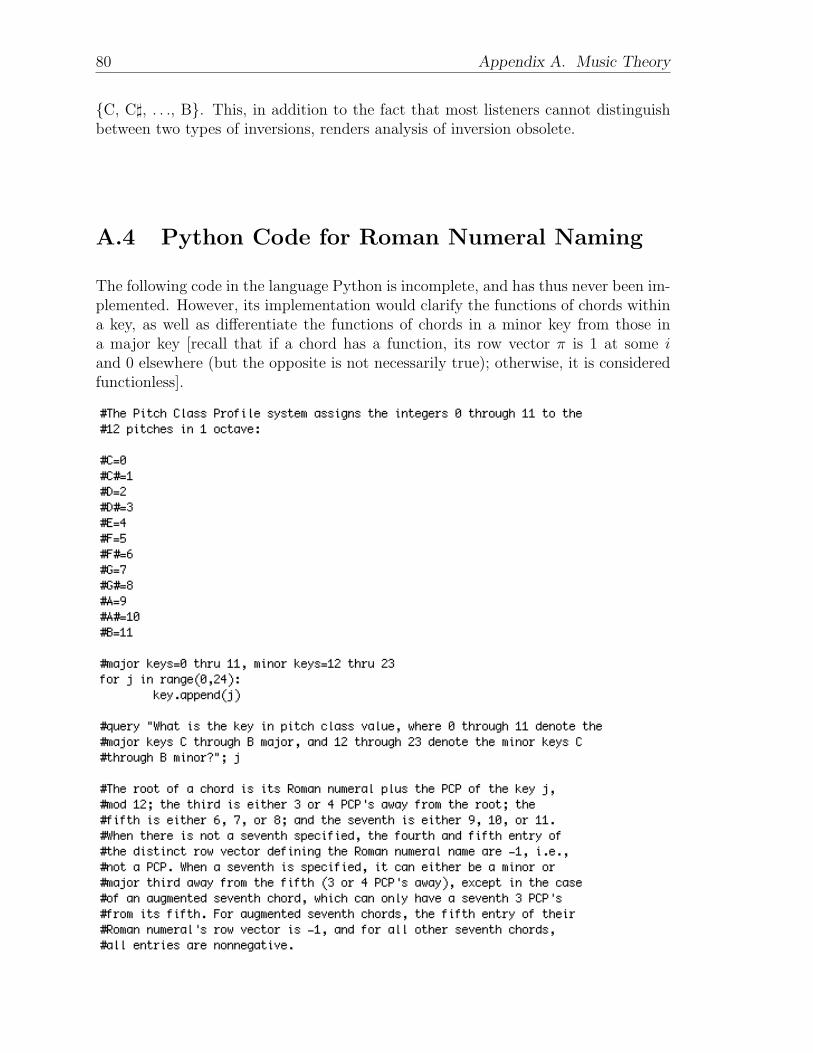
80 Appendix A. Music Theory
C, C], . . ., B. This, in addition to the fact that most listeners cannot distinguishbetween two types of inversions, renders analysis of inversion obsolete.
A.4 Python Code for Roman Numeral Naming
The following code in the language Python is incomplete, and has thus never been im-plemented. However, its implementation would clarify the functions of chords withina key, as well as differentiate the functions of chords in a minor key from those ina major key [recall that if a chord has a function, its row vector π is 1 at some iand 0 elsewhere (but the opposite is not necessarily true); otherwise, it is consideredfunctionless].
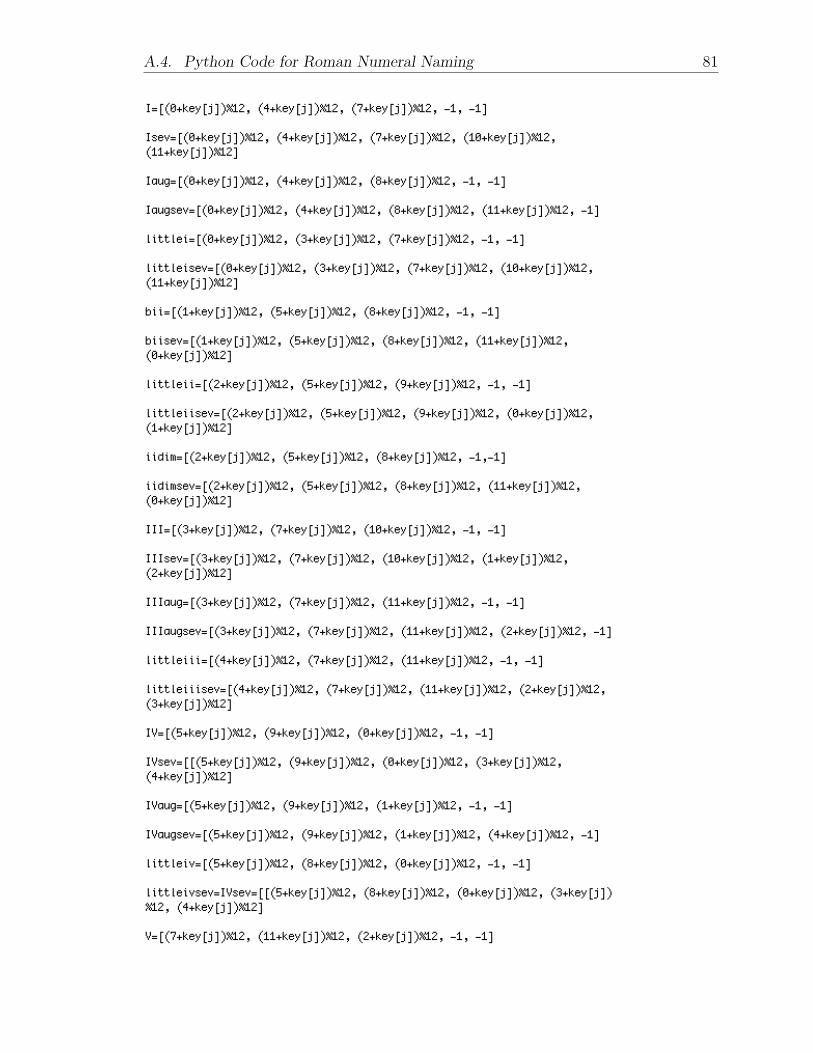
A.4. Python Code for Roman Numeral Naming 81
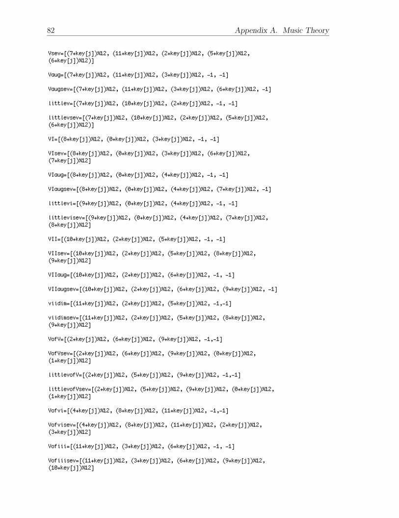
82 Appendix A. Music Theory
A.4. Python Code for Roman Numeral Naming 83

Appendix B
Hidden Markov Models
B.1 Application
We see Hidden Markov Models (HMMs) most often in research on speech recognition,but because music is inherently like language in that every artist is unique, it hasuseful application to the recognition and algorithmic composition of music. However,I did not quite figure out the reasonable place for HMMs in chord recognition whenone does not wish to compose a song from the data, so I relocated this section to anappendix to avoid confusion.
B.2 Important Definitions and Algorithms
Definition: Hidden Markov Chain. A hidden Markov chain consists of twosequences of states, assigned to integer values: a predicted Markov chain Q =(q1, . . . , qT ) to be modified, and a sequence of observations O = (o1, . . . , oT ), where otis an observation about state qt (Landecker). The Markov property holds so that
P (qt = xt|q1 = x1, q2 = x2, . . . , qt−1 = xt−1) = P (qt = xt|qt−1 = xt−1).
So in our case with chord progressions deducing something about musical style, wethink of qi as a chord within a given style at time i, and oi as the actual (observed)chord played at time i. Since we want to predict the behavior of the chords within astyle, we construct a model that will tell us how closely O adheres to Q. This model,a hidden Markov model, is defined by the following.
Definition: Hidden Markov Model. A hidden Markov model (HMM) λ =(A,B, π) is a triple containing three different sets of probabilities: (1) the state tran-sition probabilities aij, (2) the probabilities of observing each ot given qt (defining theobservation matrix B), and (3) the probabilities of beginning the chain in each of thestates qi (the initial distributions πi).
We can think of λ as a set of parameters to be modified again and again untilP (O|λ) is maximized.
86 Appendix B. Hidden Markov Models
There are three main obstacles one must overcome to build a satisfactory HMM:
1. Given O and λ, calculate P (O|λ).
2. Given O and λ, how can we “refresh” Q so that P (Q|O, λ) is maximized?
3. Given O, alter λ to maximize P (O|λ).
We surmount the first of these problems with the forward algorithm, the second withthe Viterbi algorithm or backward algorithm, and the third can be solved with any ofthe backward-forward algorithm (sometimes called the forward-backward algorithm),the Baum-Welch algorithm, or the Expectation Maximization (EM) algorithm. Themost common and best for speech recognition is the Baum-Welch, so I believe sincemusic is a language, what with all of its “speakers” communicating distinctly (therebymaking the possibilities for the set S infinite, but the established vocabulary Q finite),it will also be best suited for music. These algorithms will be explicated once we layout more formal definitions for the many variables designated above.
Now, let there be N distinct possible states, i.e., chords, and define the statespace as S = si, 1 ≤ i ≤ N . Let there be M distinct possible observations, anddefine the observation space as V = vi, 1 ≤ i ≤ M . Then, each state qi comesfrom S, and each observation oi comes from V .
We represent the random variable of the observation at time t by Ot, and likewisethe random variable of the state at time t by Qt, such that there are T -many randomvariables for each of O and Q. By the Markov property, the probability of being in astate depends only on the previous state, and the current observation depends onlyupon the current state, so therefore,
P (Qt = qt|Q1 = q1, . . . , QT = qT , O1 = o1, . . . , OT = oT , λ) = P (Qt = qt|Qt−1 = qt−1, λ)
and
P (Ot = ot|Q1 = q1, . . . , QT = qT , O1 = o1, . . . , OT = oT , λ) = P (Ot = ot|Qt = qt, λ)
Without loss of generality, the above (beastly) equalities are notationally equivalent(in this thesis, unless otherwise noted) to writing
P (qt|q1, . . . , qT , o1, . . . , oT , λ) = P (qt|qt−1, λ),
and
P (qt|q1, . . . , qT , o1, . . . , oT , λ) = P (ot|qt, λ).
We construct our state transition matrix A, relating to Q’s behavior over time,with the probabilities
A = aij : aij = P (qt = sj|qt−1 = si, λ), 1 < t ≤ T,
N∑j=1
aij = 1.
B.2. Important Definitions and Algorithms 87
At initialization of our hidden Markov chain Q, or when t = 1, we define the initialdistribution π by the row matrix
π = πi : πi = P (q1 = si|λ),
N∑i=1
πi = 1.
Then, our observation matrix B is given by
B = bij : bij = P (ot = vj|qt = si, λ),
M∑j=1
bij = 1,
and contains the probabilities
bi(j) = bij = P (ot = vj|qt = si, λ),
bqt(ot) = bqtot = P (Ot = ot|Qt = qt, λ).
We assume that A and B are time-homogenous, that is, the probability of transi-tioning between any two states is the same at all times. This is also a byproduct ofthe Markov property.
Now we can attempt to tackle the aforementioned three main problems that, oncesolved, will only better our HMM. First, we want to know how well our current modelλ predicts O, i.e., P (O|λ). Naively, this is
P (O|λ) =T∑i=1
P (O|qi, λ)P (qi|λ)
by Bayes’ formula. Now,
P (O|Q, λ) =T∏i=1
P (oi|qi, λ)
= bq1(o1) · bq2(o2) · · · bqT (oT ),
and
P (Q|λ) = πq1 · aq1q2 · aq2q3 · · · aq(T−1)qT ,
so the probability P (O|λ) becomes
T∑i=1
P (O|qi, λ)P (qi|λ) =T∑i=1
πqibq1(o1)aq1q2 · · · bqT (oT )aq(T−1)qT .
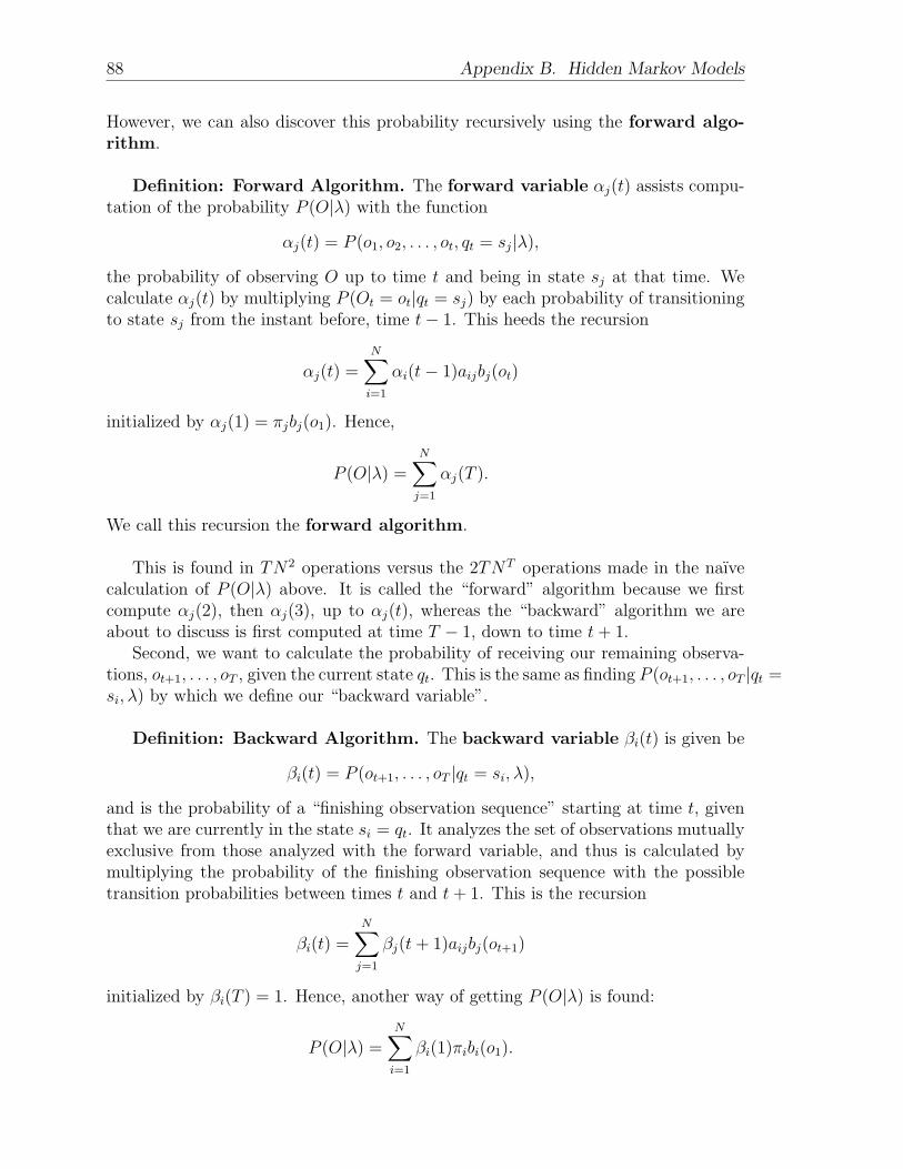
88 Appendix B. Hidden Markov Models
However, we can also discover this probability recursively using the forward algo-rithm.
Definition: Forward Algorithm. The forward variable αj(t) assists compu-tation of the probability P (O|λ) with the function
αj(t) = P (o1, o2, . . . , ot, qt = sj|λ),
the probability of observing O up to time t and being in state sj at that time. Wecalculate αj(t) by multiplying P (Ot = ot|qt = sj) by each probability of transitioningto state sj from the instant before, time t− 1. This heeds the recursion
αj(t) =N∑i=1
αi(t− 1)aijbj(ot)
initialized by αj(1) = πjbj(o1). Hence,
P (O|λ) =N∑j=1
αj(T ).
We call this recursion the forward algorithm.
This is found in TN2 operations versus the 2TNT operations made in the naıvecalculation of P (O|λ) above. It is called the “forward” algorithm because we firstcompute αj(2), then αj(3), up to αj(t), whereas the “backward” algorithm we areabout to discuss is first computed at time T − 1, down to time t+ 1.
Second, we want to calculate the probability of receiving our remaining observa-tions, ot+1, . . . , oT , given the current state qt. This is the same as finding P (ot+1, . . . , oT |qt =si, λ) by which we define our “backward variable”.
Definition: Backward Algorithm. The backward variable βi(t) is given be
βi(t) = P (ot+1, . . . , oT |qt = si, λ),
and is the probability of a “finishing observation sequence” starting at time t, giventhat we are currently in the state si = qt. It analyzes the set of observations mutuallyexclusive from those analyzed with the forward variable, and thus is calculated bymultiplying the probability of the finishing observation sequence with the possibletransition probabilities between times t and t+ 1. This is the recursion
βi(t) =N∑j=1
βj(t+ 1)aijbj(ot+1)
initialized by βi(T ) = 1. Hence, another way of getting P (O|λ) is found:
P (O|λ) =N∑i=1
βi(1)πibi(o1).
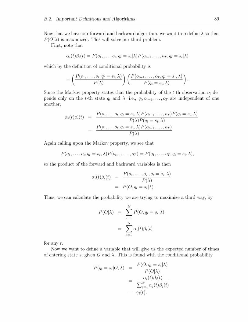
B.2. Important Definitions and Algorithms 89
Now that we have our forward and backward algorithm, we want to redefine λ so thatP (O|λ) is maximized. This will solve our third problem.
First, note that
αi(t)βi(t) = P (o1, . . . , ot, qt = si|λ)P (ot+1, . . . , oT , qt = si|λ)
which by the definition of conditional probability is
=
(P (o1, . . . , ot, qt = si, λ)
P (λ)
)(P (ot+1, . . . , oT , qt = si, λ)
P (qt = si, λ)
).
Since the Markov property states that the probability of the t-th observation ot de-pends only on the t-th state qt and λ, i.e., qt, ot+1, . . . , oT are independent of oneanother,
αi(t)βi(t) =P (o1, . . . ot, qt = si, λ)P (ot+1, . . . , oT )P (qt = si, λ)
P (λ)P (qt = si, λ)
=P (o1, . . . ot, qt = si, λ)P (ot+1, . . . , oT )
P (λ).
Again calling upon the Markov property, we see that
P (o1, . . . , ot, qt = si, λ)P (ot+1, . . . , oT ) = P (o1, . . . , oT , qt = si, λ),
so the product of the forward and backward variables is then
αi(t)βi(t) =P (o1, . . . , oT , qt = si, λ)
P (λ)
= P (O, qt = si|λ).
Thus, we can calculate the probability we are trying to maximize a third way, by
P (O|λ) =N∑i=1
P (O, qt = si|λ)
=N∑i=1
αi(t)βi(t)
for any t.Now we want to define a variable that will give us the expected number of times
of entering state si given O and λ. This is found with the conditional probability
P (qt = si|O, λ) =P (O, qt = si|λ)
P (O|λ)
=αi(t)βi(t)∑Nj=1 αj(t)βj(t)
= γi(t).
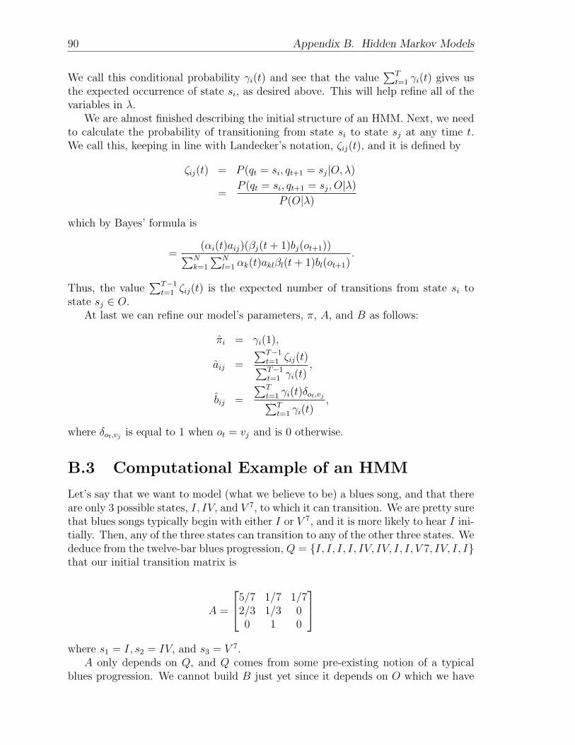
90 Appendix B. Hidden Markov Models
We call this conditional probability γi(t) and see that the value∑T
t=1 γi(t) gives usthe expected occurrence of state si, as desired above. This will help refine all of thevariables in λ.
We are almost finished describing the initial structure of an HMM. Next, we needto calculate the probability of transitioning from state si to state sj at any time t.We call this, keeping in line with Landecker’s notation, ζij(t), and it is defined by
ζij(t) = P (qt = si, qt+1 = sj|O, λ)
=P (qt = si, qt+1 = sj, O|λ)
P (O|λ)
which by Bayes’ formula is
=(αi(t)aij)(βj(t+ 1)bj(ot+1))∑N
k=1
∑Nl=1 αk(t)aklβl(t+ 1)bl(ot+1)
.
Thus, the value∑T−1
t=1 ζij(t) is the expected number of transitions from state si tostate sj ∈ O.
At last we can refine our model’s parameters, π, A, and B as follows:
πi = γi(1),
aij =
∑T−1t=1 ζij(t)∑T−1t=1 γi(t)
,
bij =
∑Tt=1 γi(t)δot,vj∑T
t=1 γi(t),
where δot,vj is equal to 1 when ot = vj and is 0 otherwise.
B.3 Computational Example of an HMM
Let’s say that we want to model (what we believe to be) a blues song, and that thereare only 3 possible states, I, IV, and V 7, to which it can transition. We are pretty surethat blues songs typically begin with either I or V 7, and it is more likely to hear I ini-tially. Then, any of the three states can transition to any of the other three states. Wededuce from the twelve-bar blues progression, Q = I, I, I, I, IV, IV, I, I, V 7, IV, I, Ithat our initial transition matrix is
A =
5/7 1/7 1/72/3 1/3 00 1 0
where s1 = I, s2 = IV, and s3 = V 7.
A only depends on Q, and Q comes from some pre-existing notion of a typicalblues progression. We cannot build B just yet since it depends on O which we have
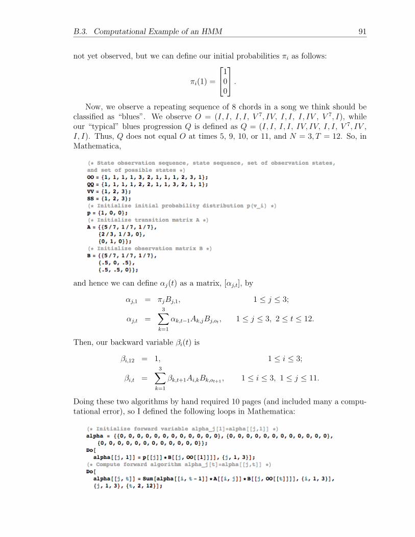
B.3. Computational Example of an HMM 91
not yet observed, but we can define our initial probabilities πi as follows:
πi(1) =
100
.Now, we observe a repeating sequence of 8 chords in a song we think should be
classified as “blues”. We observe O = (I, I, I, I, V 7, IV, I, I, I, IV , V 7, I), whileour “typical” blues progression Q is defined as Q = (I, I, I, I, IV, IV, I, I, V 7, IV ,I, I). Thus, Q does not equal O at times 5, 9, 10, or 11, and N = 3, T = 12. So, inMathematica,
and hence we can define αj(t) as a matrix, [αj,t], by
αj,1 = πjBj,1, 1 ≤ j ≤ 3;
αj,t =3∑
k=1
αk,t−1Ak,jBj,ot , 1 ≤ j ≤ 3, 2 ≤ t ≤ 12.
Then, our backward variable βi(t) is
βi,12 = 1, 1 ≤ i ≤ 3;
βi,t =3∑
k=1
βk,t+1Ai,kBk,ot+1 , 1 ≤ i ≤ 3, 1 ≤ j ≤ 11.
Doing these two algorithms by hand required 10 pages (and included many a compu-tational error), so I defined the following loops in Mathematica:
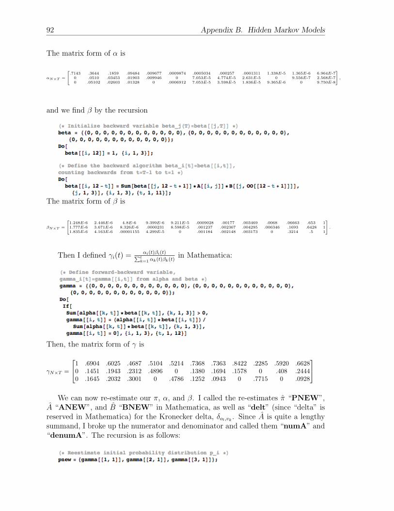
92 Appendix B. Hidden Markov Models
The matrix form of α is
αN×T =
24.7143 .3644 .1859 .09484 .009677 .0009874 .0005034 .000257 .0001311 1.338E-5 1.365E-6 6.964E-70 .0510 .03453 .01903 .009946 0 7.053E-5 4.774E-5 2.631E-5 0 9.556E-7 2.568E-70 .05102 .02603 .01328 0 .0006912 7.053E-5 3.598E-5 1.836E-5 9.365E-6 0 9.750E-8
35 ,
and we find β by the recursion
The matrix form of β is
βN×T =
241.248E-6 2.446E-6 4.8E-6 9.399E-6 9.211E-5 .0009028 .00177 .003469 .0068 .06663 .653 11.777E-6 3.671E-6 8.326E-6 .0000231 8.598E-5 .001237 .002367 .004295 .006346 .1693 .6428 11.835E-6 4.163E-6 .00001155 4.299E-5 0 .001184 .002148 .003173 0 .3214 .5 1
35 .
Then I defined γi(t) = αi(t)βi(t)Ptk=1 αk(t)βk(t)
in Mathematica:
Then, the matrix form of γ is
γN×T =
1 .6904 .6025 .4687 .5104 .5214 .7368 .7363 .8422 .2285 .5920 .66280 .1451 .1943 .2312 .4896 0 .1380 .1694 .1578 0 .408 .24440 .1645 .2032 .3001 0 .4786 .1252 .0943 0 .7715 0 .0928
We can now re-estimate our π, α, and β. I called the re-estimates π “PNEW”,
A “ANEW”, and B “BNEW” in Mathematica, as well as “delt” (since “delta” isreserved in Mathematica) for the Kronecker delta, δot,vk . Since A is quite a lengthysummand, I broke up the numerator and denominator and called them “numA” and“denumA”. The recursion is as follows:
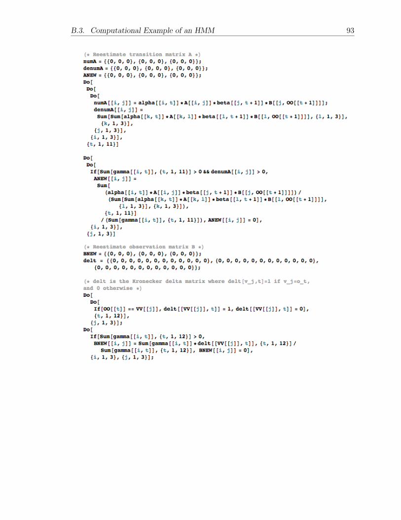
B.3. Computational Example of an HMM 93
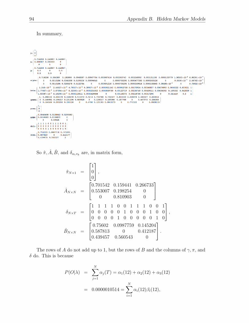
94 Appendix B. Hidden Markov Models
In summary,
So π, A, B, and δot,vk are, in matrix form,
πN×1 =
100
,AN×N =
0.701542 0.159441 0.2667330.553007 0.198254 0
0 0.810903 0
δN×T =
1 1 1 1 0 0 1 1 1 0 0 10 0 0 0 0 1 0 0 0 1 0 00 0 0 0 1 0 0 0 0 0 1 0
,BN×N =
0.75602 0.0987759 0.1452040.587813 0 0.4121870.439457 0.560543 0
.The rows of A do not add up to 1, but the rows of B and the columns of γ, π, and
δ do. This is because
P (O|λ) =N∑j=1
αj(T ) = α1(12) + α2(12) + α3(12)
= 0.0000010514 =N∑i=1
αi(12)βi(12),
B.3. Computational Example of an HMM 95
but
P (O|λ) =N∑i=1
βi(1)πibi(o1) = β1(1) · 1 · 5/7 + 0 + 0
= 0.0000008929042 =N∑i=1
αi(1)βi(1).
The failure of this very simple example perfectly encapsulates the difficulties asso-ciated with HMMs, namely with keeping all of the variables straight. A good resourcefor those unfamiliar with HMMs is [45].

Bibliography
Entropy, Information Theory, and Probability Theory
[1] Blachman, Nelson M. Noise and Its Effect on Communication. New York:McGraw-Hill, 1966.
[2] Brattain-Morrin, Eric. Entropy, Computation, and Demons. Portland, OR: 2008.
[3] Khinchin, A. I. “On the Fundamental Theorems of Information Theory ”. Math-ematical Foundations of Information Theory. New York: Dover Publications,Inc., 1957, pp. 30-120.
[4] Khinchin, A. I. “The Entropy Concept in Probability Theory. ”MathematicalFoundations of Information Theory. New York: Dover Publications, Inc., 1957,pp. 2-29.
[5] Ross, Sheldon. A First Course in Probability, Seventh Edition. Upper SaddleRiver, NJ: Pearson Education, Inc., 2006, pp. 24-26, 66-87, 132, 138-141, 205-206, 209, 214, 466-483.
[6] Shannon, Claude E. and Warren Weaver. The Mathematical Theory of Commu-nication. Urbana, IL: University of Illinois Press, 1998.
Digital Signal Processing
[7] Fleet, D.J. and A.D. Jepson. “Linear Filters, Sampling, and Fourier Analysis.”http://www.cs.toronto.edu/pub/jepson/teaching/vision/2503/, last modified 22September 2005.
[8] Johnson, Johnny R. Introduction to Digital Signal Processing. New Delhi, India:Prentice-Hall of India, 1998.
[9] Lane, John and Garth Hillman. Motorola Digital Signal Processing: Implement-ing IIR/FIR Filters with Motorola’s DSP56000/DSP56001. Motorola Inc., 1993.
[10] Marven, Craig and Gillian Ewers. A Simple Approach to Digital Signal Process-ing. New York: John Wiley and Sons, Inc., 1996, pp. 31-189.
[11] Ed. Rabiner, Lawrence R. and Charles M. Rader. Digital Signal Processing. NewYork: The Institute of Electrical and Electronics Engineers, Inc., 1972.
98 Bibliography
[12] Rabiner, Lawrence and Bing-Hwang Juang. Fundamentals of Speech Recognition.Englewood Cliffs, NJ: PTR Prentice-Hall, Inc.
[13] Roads, Curtis. The Computer Music Tutorial. Cambridge, MA: The MIT Press,1996, pp. 189, 193-196, 506-520, 934-935..
[14] Rorabaugh, C. Britton. DSP Primer. New York: McGraw-Hill, 1999.
Music
[15] Ames, C. and M. Domino. “Cybernetic Composer: An Overview”. Balaban,Mira, Kemal Ebcioglu, and Otto Laske Ed.’s. Understanding Music with AI:Perspectives on Music Cognition. Cambridge, MA: The AAAI Press/The MITPress, 1992, pp. 186-205.
[16] “Beatles Unknown ‘A Hard Day’s Night’ Chord Mystery Solved Us-ing Fourier Transform.” Updated October 2008. Accessed April 2009.http://www.scientificblogging.com/news_releases/beatles_unknown_
hard_days_night_chord_mystery_solved_using_fourier_transform?
[17] Cope, D. “On the Algorithmic Representation of Musical Style.” Balaban, Mira,Kemal Ebcioglu, and Otto Laske Ed.’s. Understanding Music with AI: Perspec-tives on Music Cognition. Cambridge, MA: The AAAI Press/The MIT Press,1992, pp. 354-363.
[18] Courtot, F. “Logical Representation and Induction for Computer Assisted Com-position.” Ed. Balaban, Mira, Kemal Ebcioglu, and Otto Laske. UnderstandingMusic with AI: Perspectives on Music Cognition. Cambridge, MA: The AAAIPress/The MIT Press, 1992, pp. 156-181.
[19] Duckworth, William. 20/20: 20 New Sounds of the 20th Century. New York:Schirmer Books, 1999.
[20] Ebcioglu, K. “An Expert System for Harmonizing Chorales in the Style of J.S.Bach.” Balaban, Mira, Kemal Ebcioglu, and Otto Laske Ed.’s. UnderstandingMusic with AI: Perspectives on Music Cognition. Cambridge, MA: The AAAIPress/The MIT Press, 1992, pp. 294-334.
[21] Gelbart, Matthew. The Invention of “Folk Music” and “Art Music”: EmergingCategories from Ossian to Wagner. Cambridge, UK: The Cambridge UniversityPress, 2007, pp. 1-6.
[22] Isacoff, Stuart. Temperament. New York: Alfred A. Knopf, 2001.
[23] Kugel, P. “Beyond Computational Musicology.” Balaban, Mira, Kemal Ebcioglu,and Otto Laske Ed.’s. Understanding Music with AI: Perspectives on Music Cog-nition. Cambridge, MA: The AAAI Press/The MIT Press, 1992, pp. 30-48.
Bibliography 99
[24] Laske, O. “Artificial Intelligence and Music: A Cornerstone of Cognitive Musi-cology.” Balaban, Mira, Kemal Ebcioglu, and Otto Laske Ed.’s. UnderstandingMusic with AI: Perspectives on Music Cognition. Cambridge, MA: The AAAIPress/The MIT Press, 1992, pp. 3-29.
[25] Lee, Kyogu. “Automatic Chord Recognition from Audio Using Enhanced PitchClass Profile.” Stanford, CA: Center for Computer Research in Music and Acous-tics, 2006, 8 pages.
[26] Maxwell, H.J. “An Expert System for Harmonic Analysis of Tonal Music.” Bal-aban, Mira, Kemal Ebcioglu, and Otto Laske Ed.’s. Understanding Music withAI: Perspectives on Music Cognition. Cambridge, MA: The AAAI Press/TheMIT Press, 1992, pp. 335-353.
[27] Rooksby, Rikky. The Beatles Complete Chord Songbook. Milwaukee, WI: H.Leonard Corp., 1999.
[28] Rowe, Robert. Interactive Music Systems: Machine Listening and Composing.Cambridge, MA: The MIT Press, 1993.
[29] Schoenberg, Arnold. Structural Functions of Harmony. London: Williams andNorgate Limited, 1954.
[30] Stephenson, Ken. What to Listen for in Rock: A Stylistic Analysis. New Haven,CT: Yale University Press, 2002.
[31] Sullivan, Anna T. The Seventh Dragon: The Riddle of Equal Temperament. LakeOswego, OR: Metamorphous Press, 1985.
Fourier Acoustics
[32] Cormen, Thomas, Charles Leiserson, Ronald Rivest, and Clifford Stein. Intro-duction to Algorithms, Second Edition. Cambridge, MA: The MIT Press, 2002.
[33] Smith, Julius O. Mathematics of the Discrete Fourier Transform (DFT): WithMusic and Audio Applications. Stanford, CA: Center for Computer Research inMusic and Acoustics, 2003.
[34] Zonst, Anders E. Understanding the FFT: A Tutorial on the Algorithm andSoftware for Laymen, Students, Technicians and Working Engineers. Titusville,FL: Citrus Press, 1995.
Hidden Markov Models
[35] Blunsom, Phil. “Hidden Markov Models.” Updated August 2004. Accessed April2009. www.cs.mu.oz.au/460/2004/materials/hmm-tutorial.pdf
[36] Chai, Wei and Barry Vercoe. “Folk Music Classification Using Hidden MarkovModels.” Proceedings of International Conference on Artificial Intelligence, 2001.
100 Bibliography
[37] Elliot, Robert J., Lakhdar Aggoun, and John B. Moore. Hidden Markov Models:Estimation and Control. New York: Springer-Verlag, 1995.
[38] Fraser, Andrew M. Hidden Markov Models and Dynamical Systems. Philadelphia:Society for Industrial and Applied Mathematics, 2008.
[39] Haggstrom, Olle. Finite Markov Chains and Algorithmic Applications. Cam-bridge, MA: Cambridge University Press, 2002.
[40] Landecker, Will. Convergence of the Baum Welch Algorithm and Applications toMusic. Portland, OR: 2007.
[41] Lee, Kyogu and Malcolm Slaney. “A Unified System for Chord Transcription andKey Extraction Using Hidden Markov Models,” in Proceedings of InternationalConference on Music Information Retrieval, 2007.
[42] Raphael, Christopher and Josh Stoddard. “Harmonic Analysis with ProbabilisticGraphical Models”. International Symposium on Information Retrieval, 2003.Ed. Holger Hoos and David Bainbridge. Baltimore: 2003, pp. 177-181.
[43] Sheh, Alexander and Daniel P.W. Ellis. “Chord Segmentation and RecognitionUsing EM-Trained Hidden Markov Models” in Proceedings of the First ACMWorkshop on Audio and Music Computing Multimedia, 2006, pp. 11-20.
[44] Takeda, Haruto, Naoki Saito, Tomoshi Otsuki, Mitsuru Nakai, Hiroshi Shi-modaira, Shigeki Sagayama. “Hidden Markov Model for Automatic Transcriptionof MIDI Signals” in IEEE Workshop on Multimedia Signal Processing, Dec. 9-11,2002, pp. 428-431.
[45] “What is a Hidden Markov Model?” Updated May 2008. Ac-cessed April 2009. http://intoverflow.wordpress.com/2008/05/27/
what-is-a-hidden-markov-model/
Glossary
accelerated intelligence Raymond Kurzweil states that “accelerated intelligence”refers to “the quickening pace of our knowledge and intelligence will ultimatelyalter the nature of what it means to be human.”
aliasing when an analog signal is undersampled to a digital form, i.e., when thesampling frequency fs < 2fU , where fU is the highest frequency (bandwidth)of the signal, the digital form undergoes aliasing, emitting false amplitudes forthe signal at frequencies n · fs, n ∈ Z
bandwidth the maximum frequency of a signal, denoted fU or W (Shannon)
conditional probability the probability of something happening given informationabout previous happenings
cyclic convolution a binary operation with no multiplicative inverse denoted by∗; the cyclic convolution of a0, . . . , aN−1 and b0, . . . , bN−1 is the sequencec0, . . . , cN−1 where
N−1∑j=0
c0xj ≡
(N−1∑j=0
ajxj
)(N−1∑j=0
bjxj
)(modxN − 1
).
dominant the frequency 7 half steps above the key to which it has a dominantrelationship
entropy a measure of the propensity of a signal or system of signals to be incorrectlytransmitted as intended
Euler’s identity eiπ = −1, where e is Euler’s number, the base of the naturallogarithm; i is the imaginary unit equal to
√−1; and π is the ratio of the
circumference of a circle to its diameter. Also, eix = cos(x) + i sin(x) ande−ix = cos(x)− i sin(x) for any value (real or imaginary) x
event in probability theory, an event is a set of outcomes
expectation in probability theory, the expectation, or expected value, of a randomvariable is the predicted value that, on average, the variable will take on
102 Glossary
fifth the frequency either 6, 7, or 8 half steps above the fundamental frequency ofa chord. This can also refer to an interval separating two notes by 6, 7, or 8half steps, depending if the quality of the interval is (respectively) diminished,perfect, or augmented
filter in digital and analog signal processing, filters are used to reduce a signal tosome desired set of frequencies
impulse in physics, impulse is the integral of force with respect to time, equal to thechange in momentum over time
impulse function δ(t)
impulse response a function h(t) mapping the power of a signal over time
independence in probability theory, two schemes or events or outcomes are inde-pendent if the occurrence of one does not effect the behavior of the other
Markov chain a Markov chain, or Markov process, is a stochastic process that pos-sesses the Markov property, and its behavior is modeled by a transition graphand transition matrix
Markov property in probability theory, a random variable is said to possess theMarkov property, or memoryless property, if every state Xt = sj only dependson the previous state Xt − 1 = si
outcome in probability theory, an outcome is a possible value of a random process,so, one state in its state space
parallel in music theory, the parallel minor key of a major key is the minor key withthe same root as the major key but different scale degrees to reflect the minorquality; the parallel major key of a minor key is likewise the major key withthe same root as the minor key but with scale degrees (staff) to represent themajor quality
probability mass function (pmf) the function describing the individual proba-bilities of every outcome in a system
quality in music theory, the nature of a chord, limited to major, minor, diminishedand augmented. Chords with major quality have their third 4 half steps abovethe root and fifth 7 half steps above the root; those with minor quality havetheir third 3 half steps above the root and fifth 7 half steps above the root;diminished chords have a third 3 half steps above the root and fifth 6 half stepsabove the root; and augmented chords are characterized by a third 4 half stepsabove the root and a fifth 8 half steps above the root. “Quality” can also applyto intervals; for instance, a major second is 2 half steps above the root while aminor second is only 1 half step above the root
Glossary 103
root the fundamental frequency of a chord, after which it is labeled with a Romannumeral
root of unity the nth roots of unity are defined as the set of all complex numbersthat are 1 when raised to the power n. These are also called de Moivre numbers
scale degree an integer denoted n is called the nth scale degree of some scale, wheren is the nth note in the scale
spectrum the positive real function of a variable f denoting frequency representingthe Fourier transform of a signal over time
state space the possible values a random process X can take on, also thought of asits range
tap a frequency in the spectrum X(f) of a signal x(t) at which the impulse responseis to be evaluated
third the frequency either 3 or 4 half steps above the fundamental frequency of achord. This can also refer to an interval separating two notes by 3 or 4 halfsteps, depending if the quality of the interval is (respectively) minor or major