The End of the Great The End of the Great Depression 1939-41: VAR Depression 1939-41: VAR

Insight onInsight onPolicy ContributionsPolicy Contributions and Fiscal Multiplier and Fiscal Multiplier

Robert J. Gordon and Robert KrennRobert J. Gordon and Robert Krenn

Northwestern University and NBER; Spot Trading LLCNorthwestern University and NBER; Spot Trading LLCThe All-UC Group in Economic History

Honors Richard Sutch and Susan B. Carter,Berkeley April 30, 2010

Three Big Questions Three Big Questions about the Great about the Great

DepressionDepression Why it happened at all? 1929-33Why it happened at all? 1929-33 Why it lasted so long, 1933-41Why it lasted so long, 1933-41 Why it eventually ended, 1939-41Why it eventually ended, 1939-41 This paper is about the third of these This paper is about the third of these

topics, with partial implications for the topics, with partial implications for the second topicsecond topic

The Obama Administration’s top The Obama Administration’s top economists all have published economists all have published positions: Summers, Bernanke, and C. positions: Summers, Bernanke, and C. RomerRomer

Our Paper Attempts to Our Paper Attempts to Replace Polemics by Replace Polemics by

ScienceScience C. Romer (1992). “Only money C. Romer (1992). “Only money

mattered” and fiscal policy had no mattered” and fiscal policy had no role in ending the Great Depressionrole in ending the Great Depression

Vernon (1994) “after 1940 only fiscal Vernon (1994) “after 1940 only fiscal expansion mattered”expansion mattered”

Bernanke and Summers-deLong: the Bernanke and Summers-deLong: the economy recovered through mean-economy recovered through mean-reversion. A non-starter, why mean reversion. A non-starter, why mean reversion in 1939-41 instead of 1933-reversion in 1939-41 instead of 1933-35?35?

This Paper Makes SixThis Paper Makes SixContributionsContributions

(1) New quarterly (and monthly) data set (1) New quarterly (and monthly) data set for components on spending on real GDP, for components on spending on real GDP, 1919-51. Avoid adding-up problem of 1919-51. Avoid adding-up problem of chain-weighted GDP by using $1937chain-weighted GDP by using $1937

(2) New criterion for “end of Great (2) New criterion for “end of Great Depression” based on a new estimate of Depression” based on a new estimate of potential real GDP for 1919-51potential real GDP for 1919-51

(3) Rejection of nonsensical “band pass (3) Rejection of nonsensical “band pass filter” estimates of GDP trend for the filter” estimates of GDP trend for the interwar period. These methods imply interwar period. These methods imply ludicrously implausible variation in the ludicrously implausible variation in the growth rate of potential outputgrowth rate of potential output

Contribution #4 Contribution #4

(4) Review of contemporary 1940-41 (4) Review of contemporary 1940-41 print media print media – To document the fact that the fiscal To document the fact that the fiscal

stimulus of WWII began in June 1940, not stimulus of WWII began in June 1940, not December 1941. December 1941.

– To document that capacity constraints in To document that capacity constraints in the last half of 1941 taint estimates of the last half of 1941 taint estimates of fiscal multipliersfiscal multipliers

– Puts perspective on the preceding Puts perspective on the preceding academic literature, reviewed in Part 4. academic literature, reviewed in Part 4.

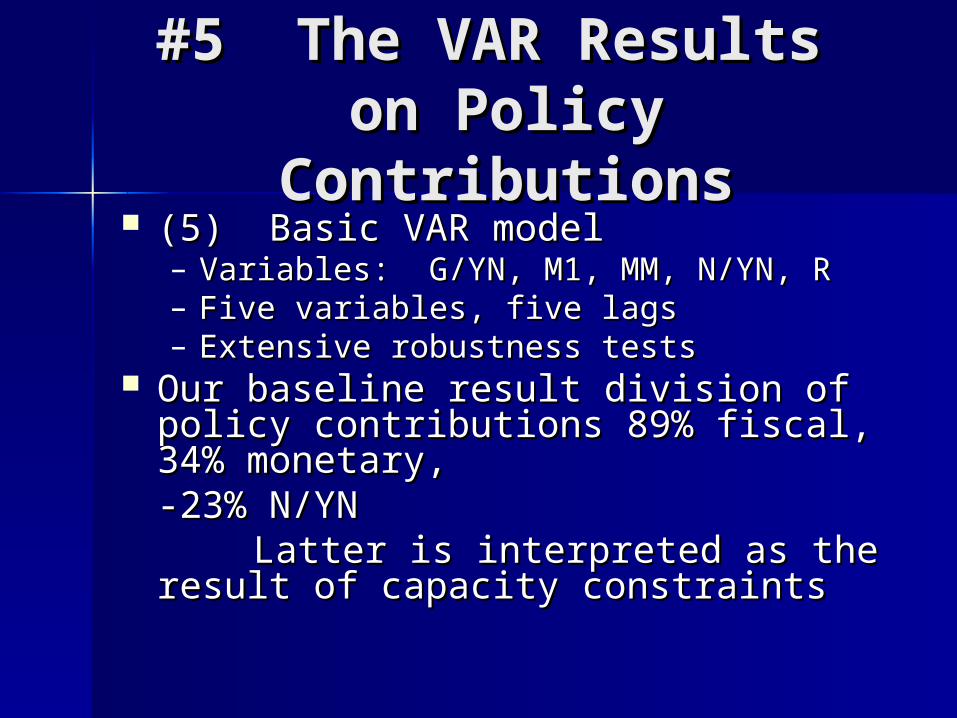
#5 The VAR Results #5 The VAR Results on Policy Contributionson Policy Contributions (5) Basic VAR model (5) Basic VAR model

– Variables: G/YN, M1, MM, N/YN, RVariables: G/YN, M1, MM, N/YN, R– Five variables, five lagsFive variables, five lags– Extensive robustness testsExtensive robustness tests

Our baseline result division of policy Our baseline result division of policy contributions 89% fiscal, 34% contributions 89% fiscal, 34% monetary, monetary, -23% N/YN -23% N/YN

Latter is interpreted as the result Latter is interpreted as the result of capacity constraintsof capacity constraints

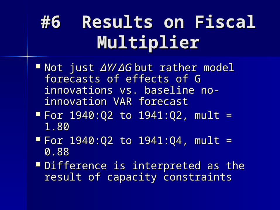
#6 Results on Fiscal #6 Results on Fiscal MultiplierMultiplier

Not just Not just ΔΔY/ Y/ ΔΔG G but rather model but rather model forecasts of effects of G innovations forecasts of effects of G innovations vs. baseline no-innovation VAR vs. baseline no-innovation VAR forecastforecast

For 1940:Q2 to 1941:Q2, mult = 1.80For 1940:Q2 to 1941:Q2, mult = 1.80 For 1940:Q2 to 1941:Q4, mult = 0.88For 1940:Q2 to 1941:Q4, mult = 0.88 Difference is interpreted as the result Difference is interpreted as the result

of capacity constraintsof capacity constraints

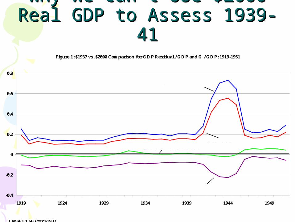
Why We Can’t Use $2000 Why We Can’t Use $2000 Real GDP to Assess 1939-41Real GDP to Assess 1939-41

Figure 1: $1937 vs. $2000 Comparison for GDP Residual / GDP and G / GDP: 1919-1951

-0.4

-0.2

0

0.2

0.4

0.6

0.8

1919 1924 1929 1934 1939 1944 1949

$2000 G / GDP

$2000 GDP Residual / GDP

$1937 GDP Residual / GDP

$1937 G / GDP

Source: 1919-1929 annual data from Balke and Gordon (1989), ratio-linked in 1929 to annual data from BEA NIPA Table 1.1.6 for $2000, ratio-linked in 1929 to annual data from BEA NIPA Table 1.1.6A (which is reverse ratio-linked in 1947 to NIPA Table 1.1.6B) for $1937

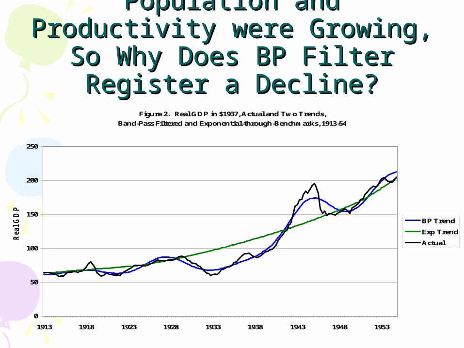
Population and Productivity Population and Productivity were Growing, So Why Does BP were Growing, So Why Does BP

Filter Register a Decline?Filter Register a Decline?Figure 2. Real GDP in $1937, Actual and Two Trends,

Band-Pass Filtered and Exponential-through-Benchmarks, 1913-54

0

50

100

150

200

250

1913 1918 1923 1928 1933 1938 1943 1948 1953

Real G

DP in

BP Trend

Exp Trend

Actual

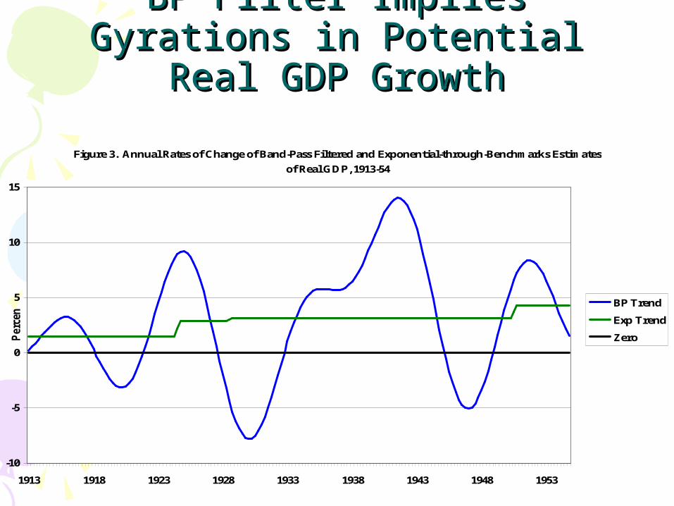
BP Filter Implies Gyrations in BP Filter Implies Gyrations in Potential Real GDP GrowthPotential Real GDP Growth

Figure 3. Annual Rates of Change of Band-Pass Filtered and Exponential-through-Benchmarks Estimates

of Real GDP, 1913-54

-10

-5

0

5

10

15

1913 1918 1923 1928 1933 1938 1943 1948 1953

Per

cent BP Trend

Exp Trend

Zero

According to BP Filter, the Log Output According to BP Filter, the Log Output Gap in 1930s was just like the 1920s!Gap in 1930s was just like the 1920s!

Figure 4. Percent Log Ratio of Actual to Trend Real GDP,

Band-Pass Filtered and Exponential-through-Benchmarks, 1913-54

-50

-45

-40

-35

-30

-25

-20

-15

-10

-5

0

5

10

15

20

25

30

35

1913 1918 1923 1928 1933 1938 1943 1948 1953

Percent BP Trend

Exp Trend

Zero

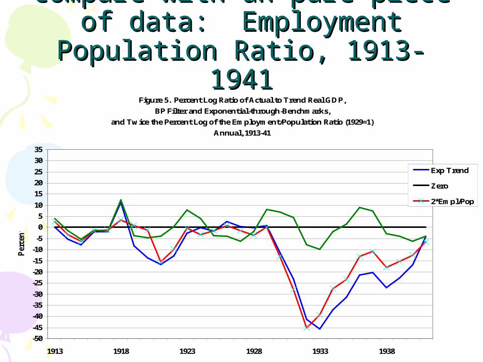
Compare with an pure piece of Compare with an pure piece of data: Employment Population data: Employment Population

Ratio, 1913-1941Ratio, 1913-1941Figure 5. Percent Log Ratio of Actual to Trend Real GDP,

BP Filter and Exponential-through-Benchmarks,

and Twice the Percent Log of the Employment/Population Ratio (1929=1),

Annual, 1913-41

-50

-45

-40

-35

-30

-25

-20

-15

-10

-5

0

5

10

15

20

25

30

35

1913 1918 1923 1928 1933 1938

Per

cent

Exp Trend

Zero

2*Empl/PopRatioBP Trend

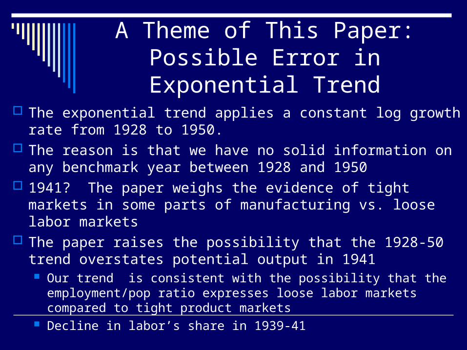
A Theme of This Paper:Possible Error in Exponential

Trend The exponential trend applies a constant log growth rate from

1928 to 1950. The reason is that we have no solid information on any

benchmark year between 1928 and 1950 1941? The paper weighs the evidence of tight markets in

some parts of manufacturing vs. loose labor markets The paper raises the possibility that the 1928-50 trend

overstates potential output in 1941 Our trend is consistent with the possibility that the employment/pop

ratio expresses loose labor markets compared to tight product markets

Decline in labor’s share in 1939-41

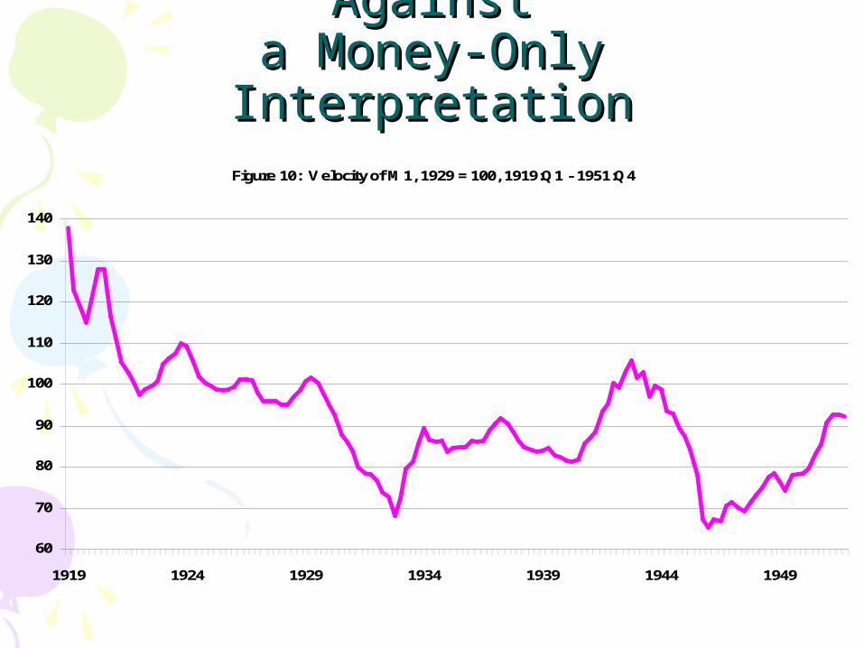
Velocity of M1 Works AgainstVelocity of M1 Works Againsta Money-Only Interpretationa Money-Only Interpretation

Figure 10: Velocity of M1, 1929 = 100, 1919:Q1 - 1951:Q4

60

70

80

90

100

110

120

130

140

1919 1924 1929 1934 1939 1944 1949

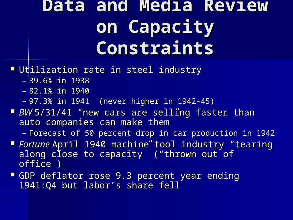
Data and Media Data and Media Review on Capacity Review on Capacity

ConstraintsConstraints Utilization rate in steel industryUtilization rate in steel industry

– 39.6% in 193839.6% in 1938– 82.1% in 194082.1% in 1940– 97.3% in 1941 (never higher in 1942-45)97.3% in 1941 (never higher in 1942-45)

BW BW 5/31/41 “new cars are selling faster than auto 5/31/41 “new cars are selling faster than auto companies can make them”companies can make them”– Forecast of 50 percent drop in car production in 1942Forecast of 50 percent drop in car production in 1942

Fortune Fortune April 1940 machine tool industry “tearing April 1940 machine tool industry “tearing along close to capacity” (“thrown out of office”)along close to capacity” (“thrown out of office”)

GDP deflator rose 9.3 percent year ending GDP deflator rose 9.3 percent year ending 1941:Q4 but labor’s share fell1941:Q4 but labor’s share fell

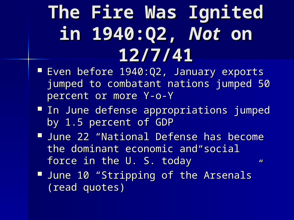
The Fire Was Ignited in The Fire Was Ignited in 1940:Q2, 1940:Q2, NotNot on on

12/7/4112/7/41 Even before 1940:Q2, January exports Even before 1940:Q2, January exports

jumped to combatant nations jumped 50 jumped to combatant nations jumped 50 percent or more Y-o-Ypercent or more Y-o-Y

In June defense appropriations jumped by In June defense appropriations jumped by 1.5 percent of GDP1.5 percent of GDP

June 22 “National Defense has become the June 22 “National Defense has become the dominant economic and social force in the dominant economic and social force in the U. S. today”U. S. today”

June 10 “Stripping of the Arsenals” (read June 10 “Stripping of the Arsenals” (read quotes)quotes)

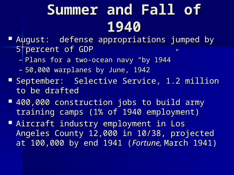
Summer and Fall of Summer and Fall of 19401940

August: defense appropriations jumped by 5 August: defense appropriations jumped by 5 percent of GDPpercent of GDP– Plans for a two-ocean navy “by 1944”Plans for a two-ocean navy “by 1944”– 50,000 warplanes by June, 194250,000 warplanes by June, 1942

September: Selective Service, 1.2 million to September: Selective Service, 1.2 million to be draftedbe drafted

400,000 construction jobs to build army 400,000 construction jobs to build army training camps (1% of 1940 employment)training camps (1% of 1940 employment)

Aircraft industry employment in Los Angeles Aircraft industry employment in Los Angeles County 12,000 in 10/38, projected at 100,000 County 12,000 in 10/38, projected at 100,000 by end 1941 (by end 1941 (Fortune, Fortune, March 1941) March 1941)

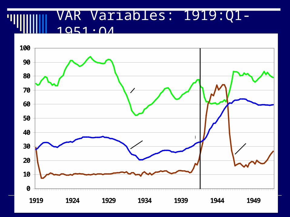
VAR Variables: 1919:Q1-1951:Q4

0

10

20

30

40

50

60

70

80

90

100

1919 1924 1929 1934 1939 1944 1949

100*(N/YN)

100*(G/YN)100*(Nominal M1/YN)

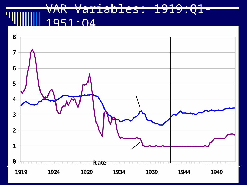
VAR Variables: 1919:Q1-1951:Q4

0

1

2

3

4

5

6

7

8

1919 1924 1929 1934 1939 1944 1949

M1 Money Multiplier

Nominal Interest

Rate

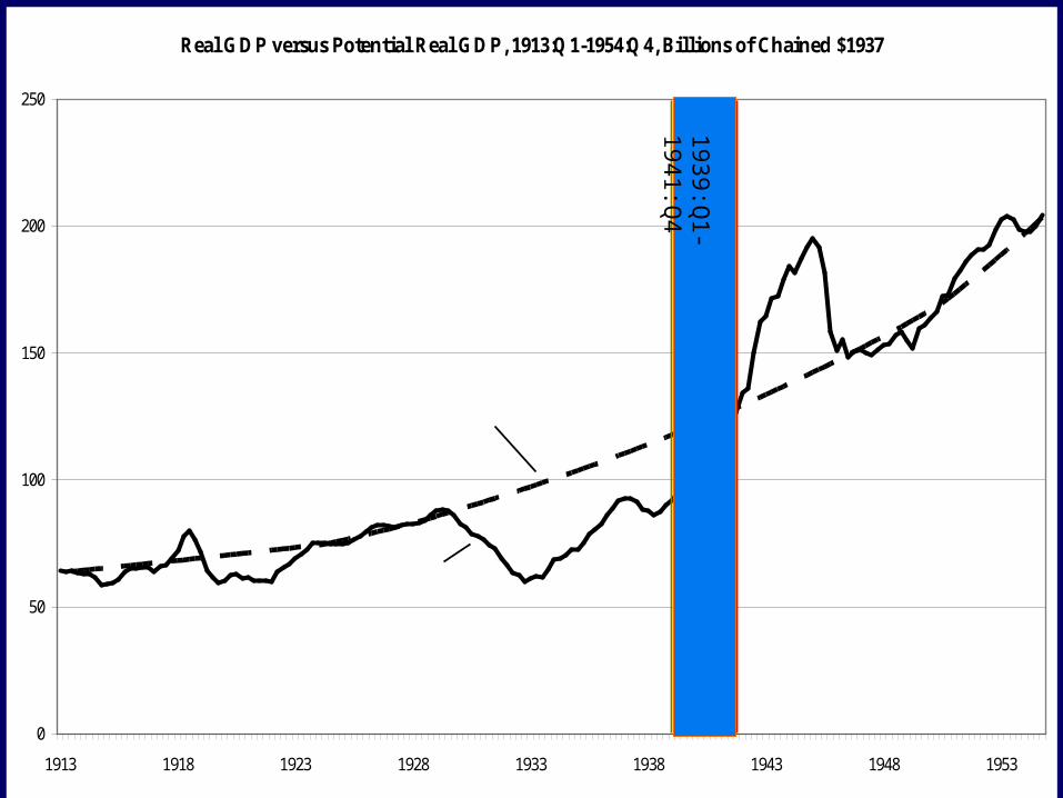
Real GDP versus Potential Real GDP, 1913:Q1-1954:Q4, Billions of Chained $1937

0

50

100

150

200

250

1913 1918 1923 1928 1933 1938 1943 1948 1953

Potential Real GDP

Real GDP

Source: See Data Appendix

19

39

:Q1

-1

94

1:Q

4

Section 6: VAR Results

We perform three main tests using VARs: historical decompositions, dynamic forecasts and impulse response functions

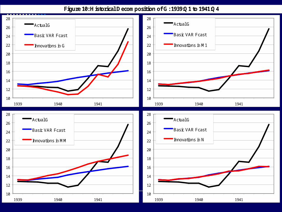
Figure 10: Historical Decomposition of G: 1939:Q1 to 1941:Q4

10

12

14

16

18

20

22

24

26

28

1939 1940 1941

Actual G

Basic VAR Fcast

Innovations in G

10

12

14

16

18

20

22

24

26

28

1939 1940 1941

Actual G

Basic VAR Fcast

Innovations in M1

10

12

14

16

18

20

22

24

26

28

1939 1940 1941

Actual G

Basic VAR Fcast

Innovations in MM

10

12

14

16

18

20

22

24

26

28

1939 1940 1941

Actual G

Basic VAR Fcast

Innovations in N

10

12

14

16

18

20

22

24

26

28

1939 1940 1941

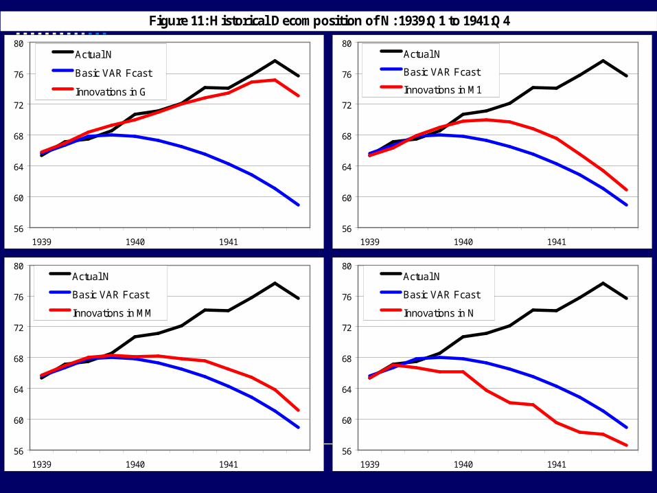
Figure 11: Historical Decomposition of N: 1939:Q1 to 1941:Q4

56

60

64

68

72

76

80

1939 1940 1941

Actual N

Basic VAR Fcast

Innovations in G

56

60

64

68

72

76

80

1939 1940 1941

Actual N

Basic VAR Fcast

Innovations in M1

56

60

64

68

72

76

80

1939 1940 1941

Actual N

Basic VAR Fcast

Innovations in MM

56

60

64

68

72

76

80

1939 1940 1941

Actual N

Basic VAR Fcast

Innovations in N

56

60

64

68

72

76

80

1939 1940 1941

Figure 12: Historical Decomposition of Y: 1939:Q1 to 1941:Q4

72

76

80

84

88

92

96

100

104

1939 1940 1941

Actual Y

Basic VAR Fcast

Innovations in G

72

76

80

84

88

92

96

100

104

1939 1940 1941

Actual Y

Basic VAR Fcast

Innovations in M1

72

76

80

84

88

92

96

100

104

1939 1940 1941

Actual Y

Basic VAR Fcast

Innovations in MM

72

76

80

84

88

92

96

100

104

1939 1940 1941

Actual Y

Basic VAR Fcast

Innovations in N

72

76

80

84

88

92

96

100

104

1939 1940 1941

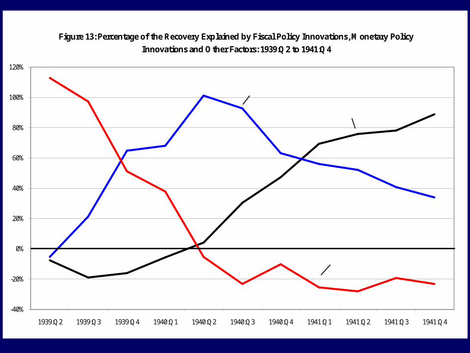
Figure 13: Percentage of the Recovery Explained by Fiscal Policy Innovations, Monetary Policy

Innovations and Other Factors: 1939:Q2 to 1941:Q4

-40%

-20%

0%

20%

40%

60%

80%

100%

120%

1939:Q2 1939:Q3 1939:Q4 1940:Q1 1940:Q2 1940:Q3 1940:Q4 1941:Q1 1941:Q2 1941:Q3 1941:Q4Source: See Data Appendix

Monetary Policy

Fiscal Policy

Other Factors

Section 7: ConclusionSection 7: Conclusion

This paper examines the recovery of the United This paper examines the recovery of the United States from the Great Depression of the 1930s, a States from the Great Depression of the 1930s, a topic that has been intensely debated by economists topic that has been intensely debated by economists in recent decades. in recent decades.

A newly created quarterly dataset of real GDP A newly created quarterly dataset of real GDP components, the GDP Deflator and potential real components, the GDP Deflator and potential real GDP allows the paper to take a fresh look at the GDP allows the paper to take a fresh look at the issue of whether fiscal or monetary policy dominated issue of whether fiscal or monetary policy dominated the recovery.the recovery.

All testing in the paper is done within a 5 variable, 5 All testing in the paper is done within a 5 variable, 5 lag VAR framework that accounts for the correlations lag VAR framework that accounts for the correlations between the variables and presents a more realistic between the variables and presents a more realistic model for the recovery period than those used in model for the recovery period than those used in previous studies. previous studies.

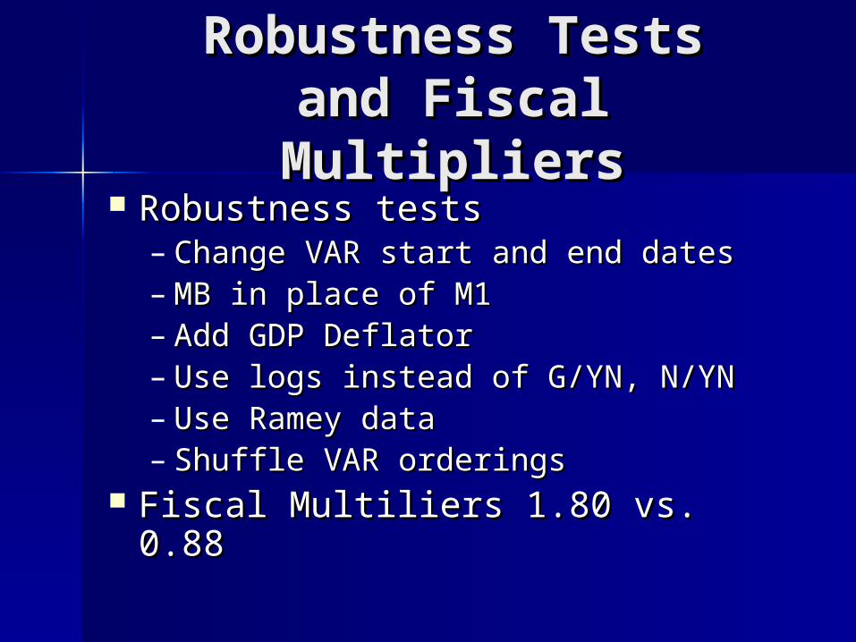
Robustness TestsRobustness Testsand Fiscal Multipliersand Fiscal Multipliers

Robustness testsRobustness tests– Change VAR start and end datesChange VAR start and end dates– MB in place of M1MB in place of M1– Add GDP DeflatorAdd GDP Deflator– Use logs instead of G/YN, N/YNUse logs instead of G/YN, N/YN– Use Ramey dataUse Ramey data– Shuffle VAR orderingsShuffle VAR orderings

Fiscal Multiliers 1.80 vs. 0.88Fiscal Multiliers 1.80 vs. 0.88

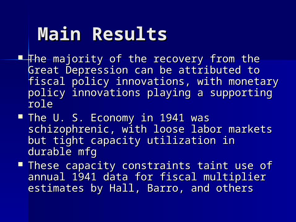
Main ResultsMain Results The majority of the recovery from the Great The majority of the recovery from the Great

Depression can be attributed to fiscal policy Depression can be attributed to fiscal policy innovations, with monetary policy innovations, with monetary policy innovations playing a supporting roleinnovations playing a supporting role

The U. S. Economy in 1941 was The U. S. Economy in 1941 was schizophrenic, with loose labor markets but schizophrenic, with loose labor markets but tight capacity utilization in durable mfgtight capacity utilization in durable mfg

These capacity constraints taint use of These capacity constraints taint use of annual 1941 data for fiscal multiplier annual 1941 data for fiscal multiplier estimates by Hall, Barro, and others estimates by Hall, Barro, and others

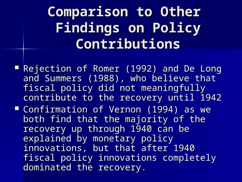
Comparison to Other Comparison to Other Findings on Policy Findings on Policy

ContributionsContributions

Rejection of Romer (1992) and De Long Rejection of Romer (1992) and De Long and Summers (1988), who believe that and Summers (1988), who believe that fiscal policy did not meaningfully fiscal policy did not meaningfully contribute to the recovery until 1942 contribute to the recovery until 1942

Confirmation of Vernon (1994) Confirmation of Vernon (1994) as we both as we both find that the majority of the recovery up find that the majority of the recovery up through 1940 can be explained by through 1940 can be explained by monetary policy innovations, but that after monetary policy innovations, but that after 1940 fiscal policy innovations completely 1940 fiscal policy innovations completely dominated the recovery.dominated the recovery.