Embed Size (px)
Citation preview
Department of Economics
THE EMPIRICAL RELEVANCE OF A BASIC STICKY-
PRICE INTERTEMPORAL MODEL
Massimo Giuliodori∗∗
University of Glasgow
Glasgow, August 2001
Abstract
In this paper, we first outline the monetary version of the sticky price intertemporal model ofObstfeld and Rogoff (1995, 1996), in which monetary shocks unambiguously generate apermanent nominal exchange rate depreciation and a temporary current account surplus. Wethen empirically investigate these theoretical predictions in two structural VAR systems for15 OECD countries over the period 1979-1999, using the long-run restriction identificationscheme suggested by Clarida and Galì (1994). Our empirical findings support the mainpredictions of the basic model, as well as suggesting that monetary shocks play an importantrole in the current account fluctuations. Moreover, we find that more open economies showgreater sensitivity of the current account to monetary shocks.
Keywords: Structural VAR, real exchange rate and current account.
JEL Classification: C32, E40, F41, F42
∗ I am grateful to Ulrich Woitek for providing the GAUSS codes and help in implementing the econometricprocedure. I also thank Jim Malley, Campbell Leith, Jordi Galì, Phillip Lane, seminar participants at theUniversity of Glasgow and discussants at the Scottish Doctoral Programme Methodology Conference 2001, theEuropean Economic Association Conference 2001 (Lousanne) and the MMF Annual Conference 2001(Belfast) for useful comments and suggestions. The usual disclaimer applies.

2
1. Introduction
Over the last two decades, many researchers have tried to provide an analytical framework,
which could be a superior alternative to the Mundell-Fleming model. To this regard, a
number of studies published in the early 1980s moved towards an “intertemporal approach”,
based on microfounded optimising models, where preferences, technology and capital
markets access are directly included.
Most of this literature, however, addresses the intertemporal analysis of the current account
determination focusing on flexible-price and non-monetary economies, in which fiscal and
technology shocks are the main sources of current account fluctuations (Glick and Rogoff,
1995 and Obstfeld and Rogoff, 1996a for a survey). Only recently, following the partial
failure of this class of models in explaining the high volatility of the current account, some
studies have introduced a role for monetary shocks as fundamental determinants of external
imbalances. The Redux model by Obstfeld and Rogoff (1995, 1996) (henceforth OR) is
without doubt considered as the precursor of this literature, which introduces market
imperfections (namely price stickiness and monopolistic competition) in an intertemporal
optimising open economy framework.1 Their model shows that, under floating exchange
rates, monetary shocks unambiguously affect consumption, income and current account.
However, the original assumptions of the OR framework have been relaxed by many
authors, who show that the main predictions are not robust to alternative hypothesis on the
key parameters (see Lane, 2001 for an excellent survey). As a result, we conduct some
empirical evidence on this direction and evaluate the relative importance of monetary shocks
in explaining real exchange rates and current account fluctuations in 15 OECD countries by
estimating two structural VARs. In order to identify the structural forces driving the variable
dynamics over the short--run, we make use of long-run identification restrictions ´ la
Blanchard and Quah (1989) and Clarida and Galì (1994).
1 For several years, the traditional aggregative Keynesian models with sticky prices and the flexible-priceintertemporal neo-classical models have represented the main way of modelling the economy. Both of them,however, present weaknesses. The former ones, although they allow for nominal rigidities, have manyshortcomings in what they lack of microfundations for intertemporal choice by ignoring the intertemporalbudget constraints, say very little about current accounts and budget deficits, and, in general, do not provide aclear description of the transmission mechanisms of the monetary and fiscal policies. Moreover, they do notallow for welfare and normative analysis which enormously limit the possibility of formulating policyprescriptions. On the other hand, the neo-classical models, while embodying many of these central issues, arestill based on the unrealistic hypothesis of flexible prices and perfectly competitive markets.

3
The aim of this study is twofold. Firstly, as pointed out by Lane (1999), this exercise can be
helpful in distinguishing between those class of models predicting a current account surplus
in response to a monetary shock (Mundell, 1983 and Obstfeld and Rogoff, 1995, 1996
among others), and those in which a current account neutrality or deficit might occur as in
Betts and Devereux (1996, 2000), Lombardo (2001), Kollmann (1997) and Chari, Kehoe and
McGrattan (1997), Tille (2001). A second aim is to investigate the role of nominal or
monetary shocks in the understanding of the current account determination, which, in the
previous empirical analysis, has mainly been focusing on technology and fiscal shocks
(Glick and Rogoff, 1995).
The structure of the rest of the paper is organised as follows. In Section 2, we briefly outline
the monetary version of the OR model and some of its predictions. Section 3 summarises
two main extensions, which, by keeping the basic structure of the Redux model, while
introducing pricing-to-market and different degrees of elasticity of substitution between
home and foreign goods, allow for the possibility of different qualitative implications.
Section 4 provides an overview of some recent empirical attempts to test the role of
monetary shocks on exchange rate and current account determination. Section 5 outlines the
econometric approach we use, while Section 6 comments on the specifications and provides
the estimation results. Section 7 concludes.
2. A Basic Two-Country General Equilibrium Model of International MonetaryPolicy Transmission (Obstfeld-Rogoff Redux Model, 1995, 1996)
In what follows we outline a textbook version of the Redux model in which Obstfeld and
Rogoff (1995, 1996) develop a perfect foresight two-country general equilibrium monetary
model which combines three fundamental blocks.2
1. the first emphasises the intertemporal decisions by individual agents where foreign trade
and asset exchange open up avenues for transferring resources over time which are not
available in a closed economy;
2. the second is based on monopolistic competition in the goods market, which plays a
central role because it rigorously defends the Keynesian assumption that output is
demand-determined in the short-run;
2 This outline is strongly based on the monetary version model summarised in Chapter 10 of Obstfeld andRogoff (1996) and the original paper in Obstfeld and Rogoff (1995)

4
3. the third contemplates the presence of sticky prices.
In their model, the world is populated by a continuum of individual consumer-producers,
indexed by z ∈ [0, 1], each of whom produces a single differentiated perishable good, also
indexed by z. The home country consists of producers on the interval [0, n], and the
remaining agents z ∈ (n, 1] reside in the foreign country. Thus, n provides an index of the
relative size of the two countries. Foreign variables will be denoted by a superscript asterisk
(*).
Individuals everywhere in the world have preferences defined over a consumption index,
real money balances, and effort expended in production.3 In particular, the intertemporal
utility function of a typical home agent j depends positively on consumption and real
balances, and negatively on work effort, which is positively related to output. For analytical
reasons, OR take into account the specific case, in which all individuals have the same
preferences defined by
(2.1) U CM
P
ky zt
s ts
s
ss
s t
= +−
FHG
IKJ −
LNMM
OQPP
−
−
=
∞
∑βχ
ε
ε
log ( )1 2
1
2 ,
where 0 < β < 1 is the subjective rate of discount, ε > 0 is a parameter inversely related to the
elasticity of money demand, the elasticity of intertemporal substitution is equal to 1 and the
elasticity of disutility from output equal to 2.4
Assuming that all goods are traded and letting cj(z) be a home individual’s consumption of
product z, the variable Cj can be defined as a real consumption index, on which utility
depends, and represented by the constant-elasticity-of-substitution (CES) function
(2.2) C c z dzj j=LNM
OQP
− −z ( )θθ
θθ1
0
1 1
,
where the elasticity of substitution between varieties θ > 1.5 The foreign consumption C* is
defined analogously.
3 The assumption of time-separable utility function is preferable for a number of reasons. In particular, Obstfeldand Rogoff (1996) point out that an intertemporal non-separable utility function would yield few concrete andtestable predictions, and that empirical research has not been able to provide a superior non-separablealternative.4 It is easy to show that a rise in home productivity can be captured by a fall in k.5 As pointed out by Obstfeld and Rogoff (1995) this assumption is necessary because the parameter θ is alsothe price elasticity of demand faced by each monopolist. They have to impose this restriction, because since

5
The price deflator for nominal money balances is the consumption-based money price index
corresponding to (2.2).6 Letting p(z) be the home-currency price of good z, it is easy to show
that the money price level in the home country is:
(2.3) P p z dz= LNM
OQP
− −z ( )1
0
11
1θ θ
Being p*(z) the foreign-currency price of good z, the foreign price index P* can be written
similarly.
There are no impediments or costs to trade between the countries. Letting E be the nominal
exchange rate, defined as the home-currency price of foreign currency, then the law of one
price holds for every good,7 so that
(2.4) p z Ep z( ) * ( )=
Since both countries’ residents have the same preferences, equation (2.2) implies that home
and foreign consumer price indexes are related by purchasing power parity (PPP)
(2.5) P EP= *
There is no capital or investment, but this is not an endowment economy because labour
supply is elastic. This means that period t output of good z, yt(z), is chosen in a manner that
depends on the marginal revenue of higher production, the disutility of effort, and the
marginal utility of consumption, that is, the output is endogenous.
There is an integrated world capital market in which both countries can borrow and lend.
The only asset they trade is a real bond, denominated in the composite consumption good.
Let rt be the real interest rate earned on bonds between t and t+1 and Ft and Mt the stocks of
bonds and domestic money held by a home resident entering date t+1.
marginal revenue is negative when elasticity of demand is less than 1, θ > 1 ensures an interior equilibriumwith a positive level of output. However, as pointed out by Lombardo (2001), the elasticity of substitutionbetween domestic and imported goods in OR model is "unnecessary" constrained to be bigger than one. Herelaxes this assumption providing interesting insights. Tille (2001) further extends the basic model allowing fordifferent elasticity of substitution across and within countries. See the next Section for a brief outline of theseextensions.6 The price index is defined as the nominal expenditure of domestic money needed to purchase a unit ofconsumption C.7 In this model the law of one price always holds. However, several authors (Engel, 1998 – Rogoff, 1996) havedocumented that international deviations in tradable prices are responsible for a large proportion of realexchange fluctuations. Following this empirical evidence, Betts and Devereux (1996, 1998, 2000) haveintroduced market segmentation into the basic model in the form of “pricing-to-market” (PTM). As above, thisextension produces theoretical implications in the international transmission of monetary (as well fiscal) policywhich differ from the OR model. Similarly, Chari et al. (1997) develop a sticky price model with pricediscriminating monopolists, which produces deviations from the law of one price. See the next Section for abrief discussion.

6
Individual z’s period budget constraint written in nominal terms is:
(2.6) P F M P r F M p z y z P C P Tt t t t t t t t t t t t t+ = + + + − −− − −( ) ( ) ( )1 1 1 1
where y(z) is the individual’s output, for which agent z is the only producer, and T denotes
lump-sum real taxes paid to the domestic government (which can be negative in the event of
money transfers).
Since Ricardian equivalence holds in this model, they assume that the government runs a
balanced budget each period. Therefore, all seignorage revenues are rebated to the public in
the form of transfers:
(2.7) TM M
PPT M Mt
t t
tt t t t=
+= −−
−1
1 or
The same is true for the foreign country.
Given the constant-elasticity-of-substitution consumption index, eq. (2.2), it is easy to find
the home individual j’s demand for good z in period t and the correspondent demand of a
foreign individual.
Integrating demand for good z across all agents (that is, taking a population weighted
average of home and foreign demands), and making use of eqs. (2.2) and (2.4), which
implies that p(z)/P = p*(z)/P* for any good z, we can determine the constant-elasticity-of-
substitution total world demand for good z
(2.8) y zp z
PCt
d t
ttw( )
( )=LNM
OQP
−θ
where world consumption Ctw , which producers take as given, is defined as
(2.9) C C dj C dj nC n Ctw j j
n
n
t t= + = + −zz * *( ) 1
01 ,
where they imposed symmetry on the identical agents within each country in order to
simplify notation.
From the first order condition of the utility maximisation, the following functions are
derived:
(2.10) C r Ct t t+ = +1 1β( )
(2.11) M
PC
i
it
tt
t
t
=+F
HGIKJ
LNM
OQP
χε
11/
,

7
where we use the Fischer parity equation defined as ( ) ( )1 11+ = ++iP
Prt
t
tt , and
(2.12) y zk
CCt t
w
t
( ) ( ) /θθ θθ
θ
−
=−1
11 1
which represent respectively, the standard Euler equation, the money demand and labour
supply equation. The same is true for the foreign country counterpart equations.
In order to analyse the effects of a monetary shock, they carry out a log-linear approximation
around a flexible-price steady-state equilibrium (where all the exogenous variables are
constant and where the initial stock of net foreign assets is 0, i.e. F F0 0 0= =* ) and solve
for differences between home and foreign log-linearized expressions.8
In the short-run, nominal producers prices p(h) and p*(f) are predetermined, that is, they are
set a period in advance but can be adjusted fully after one period. In this sense, we can
interpret the possible sources of stickiness with menu costs of price adjustment. With sticky
nominal prices, output becomes demand determined for small enough shocks, because the
monopolist always prices above marginal cost, and it is profitable to meet unexpected
demand shocks at the pre-set price. Since prices are fixed for one period, Obstfeld and
Rogoff distinguish between the impact (first-period) effect of a shock and its long-run
(second-period) steady-state effect.
In considering the effects of an unanticipated permanent rise in the relative home money
supply (that is, *11
* ˆˆˆˆ++ −=− tttt MMMM ) the main findings and dynamics of the model can
be summarised as follows.
A monetary expansion in the home country produces a nominal depreciation and a
subsequent rise in the domestic price level, followed by a decrease of the domestic relative
prices. As a consequence, and under the assumption of monopolistic competition, domestic
output temporarily expands. With consumption which is based on permanent income,
consumption rises less than output, leading the home country to run a current account
surplus. The excess of output over domestic consumption is exported and, as a payment for
these exports, the home country receives claims against the future output of the foreign
8 They implement this linearization by expressing the model in terms of deviations from the baseline steady-
state path. By denoting percentage changes from the baseline by hats, for any variable, $ /X dX Xt t≡ 0 ,
where X 0 is the initial steady-state value.

8
country. Domestic consumption, therefore, rises although the increase in output lasts for only
one period.
Although a full analytical description of the relevant equations would make the analysis
more thorough, the main findings, which are relevant for the theoretical relationship between
monetary policy, exchange rate and current account, can be summarised in the following
expressions.
(2.13) $ $ ( $ $ ) ( $ $ )* *E E M M C Ct t t t t t= = − − −+11ε
which shows that the exchange rate jumps immediately to its new long-run equilibrium
following a permanent relative money shock. The assumption behind this result is that if
consumption differentials and money differentials are both expected to be constant, then
agents must expect a constant exchange rate as well.
Another important equation, which derives directly from the budget constraint, is
(2.14) ( ) ( )*tttw
t CCEnC
dF−−−θ=
−1
1
1
0
which tells us that the change in bond holdings (namely, in current account) is a positive
function of the exchange rate deviation from the steady-state value (being θ >1) and a
negative function of the difference between home and foreign per capita consumption. The
first member of the RHS is a result consistent with the Marshall-Lerner condition, but in
addition we also have a consumption effect which tells us that the larger the increase of
relative consumption, the smaller the wealth transfer.9
Eq. (2.14) can be rewritten as follows
(2.15) ( )( ) ( )( )*tttEw
t CCnEnZC
dF−−−−θ−=≡ 111
0
,
where we can see that the smaller the home country (i.e. the smaller n), and the larger the
elasticity of substitution between varieties, the larger the impact on the home current
account.
The second expression derived from the model is given by
(2.16) ( ) ( )*ttw
t CCrnC
dF−
−θθ
=
− 1
2
1
1
0
,

9
which shows that the consumption change is positively related to the current account surplus
through the permanent interest income which home individuals earn from the wealth
transfer. Moreover, it is easy to see that the increase in consumption is less than the amount
dFr (since θ >1), for the fact that the higher wealth leads to some increase in leisure and,
consequently, in some reduction of production. Similarly to the expression EZ , we can
rewrite eq. (2.16) as
(2.17)( )( ) ( )*
ttCwt CC
r
nZ
C
dF−
−θ−θ
=≡1
12
0
We provide a representation of the two lines (namely, EZ and CZ ) in Figure 1. We can see
how their intersection implies that an exchange rate depreciation improves the current
account over the short run.
FIGURE 1 Effect of an unexpected home money shock on the current account.
9 This derives from the fact that under the assumption of monopolistic competition, domestic output temporaryrises. With the permanent income hypothesis, the larger is the consumption effect, which, however, expandsless that output, the smaller is the home country current account surplus.
*tt CC −
wt
C
dF
0
CZ
Z
tE

10
3. Two Extensions of the Basic Model
As originally Obstfeld and Rogoff pointed out, their framework can be improved with a
number of extensions.10 Lane (2001) offers an excellent survey of the recent literature
attempting to extend and generalise the basic Redux model by introducing sticky wages,
staggering nominal rigidities, market segmentation and pricing to market, different
household preferences and financial structures. In what follows, we provide a brief overview
of two of the most recent contributions, which, while keeping the basic structure of the
model, develop two very interesting extensions by introducing PTM and allowing for
different elasticities of substitution across and within countries. It turns out that these
assumptions strongly affect the international transmission of monetary shocks and provide
different theoretical predictions and welfare implications.
Betts and Devereux (2000) develop an extension of the OR model by allowing short-run
departures by the real exchange rate from PPP, which is assumed to hold in the basic
framework. In particular, they introduce the hypothesis that a fraction s of firms in each
country can price-discriminate across countries and, therefore, set different prices in home
and foreign markets. This parameter s provides a measure of “pricing-to-market” (PTM) in
some traded goods industries where firms tend to set prices in local currencies of sale and do
not adjust prices to movements in the exchange rate.11 Betts and Devereux (2000) show that
the nominal price stickiness and the presence of PTM increase the volatility of the exchange
rate and strongly affect the international monetary transmission mechanisms. In particular,
they show that high degree of PTM reduces the traditional “expenditure switching” effects of
exchange rate depreciation, which, as a result, has little effect on the relative price of
imported goods facing domestic consumer and on the correspondent shift in world demand.
Moreover, short-run deviations from PPP tend to generate low (with respect to models
without PTM) comovements of consumption and high positive comovements of output
across countries. The degree of PTM is clearly central to their results. In particular, they
10 For instance, they suggest introducing overlapping generations in place of homogeneous infinitely livedagents. This assumption not only allows us to have a more realistic model than the basic one, but, moresignificantly, makes room for the possibility of the Ricardian Equivalence not to hold.11 Following the lack of empirical support for the law of one price and PPP for traded goods, at least at highfrequency, in the last two decades there has been a growing literature on the presence of PTM. Glodberg andKnetter (1997) provide a comprehensive survey of the empirical evidence on the degree of exchange rate pass-through, market segmentation and pricing-to-market. Engel (1993) and Engel and Rogers (1996) provide some

11
consider the two opposite cases of s → 0 and s → 1 . In the former (i.e. the law of one price
is maintained continuously and PPP holds) for both countries, a devaluation unambiguously
improves the current account, consistently with the traditional OR model, and generates
permanent positive effects in the home consumption relative to foreign consumption. When
s → 1 and full-PTM occurs, a monetary disturbances generate exchange rate devaluation, but
no current account effects. In general, the higher the degree of PTM, a monetary shock
implies a greater exchange rate volatility, a smaller current account improvement, and
reduced permanent effects on relative consumption.12
Another simple, but crucial, extension has been developed by Tille (2001), who allows for
the elasticity of substitution across and within countries to differ and generalises the baseline
Redux model where the two parameters are equal and constrained to be bigger than one (i.e.
θ > 1 ). Under the assumption of law-of-one-price and PPP, they distinguish two possible
values of the elasticity of substitution between home and foreign goods respectively greater
and less than unity. He labels the first case as MLR (namely Marshall-Lerner-Robinson
condition), in that, when goods produced in different countries are close substitutes, an
exchange rate depreciation generates a current account surplus, a permanent rise of home
consumption relative to foreign consumption. When the goods produced in the two countries
are poor substitutes and the elasticity is less than unity (i.e. NON-MLR), the current account
will be in deficit in the short run, determining a permanent fall in relative consumption.
Similarly, Lombardo (2001) modifies the original OR specification with different degrees of
elasticity of substitution between domestic and imported goods. He derives conditions
allowing for positive, neutral and negative current account responses to a monetary
expansion and currency depreciations, arguing that the standard Marshall-Lerner condition
may not apply for specific intervals in the value of the relevant coefficients.
In summary, several models have been developed extending and generalising the basic
Obstfeld and Rogoff’s Redux model. However, the size and the sign of the effects of
monetary shocks are strongly affected by the magnitude of several key coefficients and the
structural assumptions. As pointed out by Lane (2001), the above literature has been mainly
empirical evidence and show that deviations from the law-of-one-price across international borders are greaterthan can be due to geographical distance and transportation costs.12 Similarly to Obstfeld and Rogoff (1995), Betts and Devereux (2000) also focus on the implications ofgovernment spending shocks. They show that both temporary and permanent fiscal shocks generate short-termreal depreciation and fall of relative consumption. The current account effects crucially depend on the degree of

12
focusing on theoretical aspects. However, the actual effects of monetary shocks to exchange
rates, current account and other real variables are primarily an empirical issue. While some
exercises have been mainly based on calibration methods and others on the estimation of the
key parameters of the model, a number of recent papers have addressed this deficiency by
estimating impulse-response functions generated by VAR econometric techniques, where
different identification solutions have been used. In what follows, we provide a brief
overview of the VAR empirical evidence
4. Empirical Review
The two most influential papers on which the following literature has built are Eichenbaum
and Evans (1995) (EE) and Clarida and Galì (1994) (CG). Although they use different
identification solutions, they both investigate the effects of shocks to monetary policy on
exchange rate in a manner that is qualitatively consistent with the above sticky-price models.
In particular, EE use U.S. monthly data covering the sample period 1974:1-1990:5 to
estimate alternative VAR models, which share common variables (namely, industrial
production, CPI, short-term interest rate differential and exchange rates), but differ for the
use of three measures of shocks to U.S. monetary policy.13 Their standard Cholesky
decomposition identification assumes that all shocks are orthogonalised and is such that the
monetary variables are ordered prior to the industrial production and the consumer price
level and after the interest rate and exchange rate variables. This corresponds to the
assumption that the monetary authority sets its policy instrument with current values of the
first two variables in mind, while these do not respond contemporaneously to movements of
the monetary shock. They find strong evidence that contractionary policy shocks lead to
significant and persistent appreciations in exchange rate, both nominal and real, and
conclude by pointing out that monetary shocks contributed significantly to the overall
variability of U.S. exchange rates in the post-Bretton Woods era.
PTM, the duration of the shock and the magnitude of the elasticity of labour supply. See Betts and Devereux(2000), page 233-35 for a discussion.13 They use orthogonalised shocks to the federal funds rate, orthogonalised shocks to the ratio of non-borrowedto total reserves and changes in an index they construct as monetary policy proxy.

13
Betts and Devereux (1999), by using U.S. data with respect to the remaining G-7 countries,
modify the EE’s specification, and also consider a short-run recursive identification scheme.
They find that positive innovations to monetary policy cause a sharp and persistent
depreciations of the real and nominal exchange rates.14
Lane (1999) extends the EE system to include a trade balance in order to employ data at a
monthly frequency over 1744:1-1996:12 for the U.S. with respect to other G-7 countries. In
particular, he estimates a six-variable VAR system, imposing a set of exclusion restrictions
on the contemporaneous relationship between the variables. The trade balance is ordered last
in the system to allow for contemporaneous effects of all shocks on it. However, his results
are robust to alternative orderings and two measures of the US monetary policy instrument
(i.e. the Federal Funds rate and the level of non-borrowed reserves). The impulse response
functions of the trade balance with respect to a monetary expansion show a sustained surplus
after a period of about a year, although the maximum impact occurs just after 43-48 months,
according to the monetary policy instrument used.
Another part of the VAR empirical literature has focused on the use of long-run
identification scheme á la Blanchard and Quah (1989).15 An influential contribution was
made by Clarida and Galì (1994) who investigate empirically and attempt to identify the
sources of real exchange rate movements after the collapse of Bretton Woods for the U.S.
vis-à-vis with the U.K., Germany, Japan and Canada, respectively. They make use of a
structural VAR system on output, the real exchange rate and inflation, whose long-run
identification restrictions are consistent with a stochastic version of the Obstfeld (1985) open
macro model. They assume the presence of three structural shocks to supply, demand, and
money and impose restrictions in such a manner that money shocks are expected to have no
long-run impact on either output or the real exchange rate, and the demand shock to be long-
run neutral for output.16 They find that for two of the four countries (namely, Japan and
Germany), the structural VAR estimates suggest that nominal (money) shocks explain a
substantial amount of the variance in dollar-DM and dollar-yen real exchange rates (41%
and 35% of the variance, respectively). For the U.K and Canada, variance decomposition
14 In Betts and Devereux (1996), they study a Wold decomposition a la Eichenbaum and Evans and look at theCPI responses to monetary policy shocks, which they find to be quite flat and barely significant. They interpretthese results in support of a high degree of PTM and, therefore, as if large movements in nominal exchangerates are not reflected in import prices.15 Se the next Section for an outline of this identification scheme.16 See the following Section for a description of their econometric approach.

14
results are less supportive of the monetary policy shocks relevance. However, consistent
with EE, for all countries nominal shocks lead to short-run real depreciation, a rise in U.S.
output and a jump in U.S. inflation.
A number of recent papers have made use of the CG’s VAR identification scheme, by
focusing on the current account rather that the real exchange rate, in line with the qualitative
predictions of some of the sticky-price intertemporal model. Lane (1999) estimates a three-
variable system where he takes the ratio of the U.S. and rest-of-the-world (proxied by the
non-US G-7 countries) output, the US’s current account to GDP ratio and the ratio of the
U.S. to RoW consumer price levels. He assumes that his system is driven by a sequence of
three orthogonal structural shocks, which he labels supply, absorption and monetary shocks,
respectively. His long-run identification assumptions are such that the money shock has no
long-run effects on the relative output and the current account, and the absorption shock is
long-term neutral on the relative output. The estimated IRFs of the current account to a
positive one standard deviation monetary shock show a short-term deterioration (which Lane
interprets as a J-curve effect), followed by a significant and persistent surplus which reaches
its maximum impact after 10 quarters. Quantitatively, the contribution of this shock to
current account volatility constitutes about half of its variation.
Similarly to Lane (1999), Cavallari (2001) proposes a three variable system of the ratio of
domestic to world output, the ratio of current account to output and the ratio of home to
foreign short-term interest rate. By using both short-run and long-run restrictions as in Galì
(1992), she assumes the presence of a supply, an absorption and a monetary shock. The latter
two are restricted to have no long-run effect on the output, and the monetary shock not to
affect output contemporaneously. Estimating this system over 1974:1-1997:4 for the G7
countries, she shows that the current account response to the monetary shock differs across
countries. In particular, in the case of UK, Italy, France and Canada, the current account goes
into surplus following a negative monetary shock. For the US, Germany and Japan the
reverse holds.
Prasad (1999) estimates a three variable system with the relative output level, the real
exchange rate and the ratio of trade balance to output for the G-7 countries. In particular, in
accordance with the implications of a modified version of Clarida and Galì (1994)
theoretical model, he assumes that monetary shocks have no long-run impact on the real
exchange rate and on the relative output, and that the demand shock does not affect the

15
relative output in the long run. His results show that nominal shocks appear to have played
an important role in the dynamics of the trade balance over the period 1974-1996 in G-7
countries. In particular, he shows that positive monetary shocks determine significant trade
surplus and generate positive correlations between output and trade balance.
Similarly to above, Lee and Chinn (1998) estimate an even more parsimonious two-variable
VAR model containing the real exchange rate and the ratio of the current account to GDP for
the G-7 countries, and impose a long-run neutrality restriction of a temporary (monetary)
shock on the real exchange rate. Their results are supportive of the real exchange rate
depreciation and current account surplus following a positive nominal shock.
Many of the above studies focus on transmission mechanism of the monetary shocks to the
nominal and/or real exchange rate and current account/trade imbalances mainly in the U.S.
and the remaining G7 countries. However, none of them has been applied to a wider set of
countries. In what follows, we try to fill this gap by studying the qualitative and quantitative
role of monetary shocks in the current account dynamics in a number of additional small
open economies. Several studies have shown that for non-US countries, where US and other
foreign financial and macroeconomic conditions are strictly under observation by the
respective central banks, it is necessary to modify the identification allowing for feedback
effects as well as augmenting the specification with a number of key endogenous variables in
the system (Kim, 1999, 2000; Kim and Roubini, 1999 among others). To this regard, the
VAR identification based on contemporaneous restrictions is not the most appropriate and
simple method to apply. On the basis of such considerations, we apply the identification
scheme suggested by Blanchard and Quah (1989) and Clarida and Galì (1994) and, as a
result, keep our specifications as parsimonious as possible, contemporaneously testing for
the main driving forces of current account dynamics. Before motivating our specifications
and providing the correspondent empirical results, we outline our econometric approach.
5. The Econometric Approach
The empirical strategy we implement builds on earlier work by Blanchard and Quah (1989)
and Clarida and Galì (1994), who propose an identification scheme for VARs, in which they
impose long-run restrictions on the behaviour of the variables in the system.

16
In outlining their empirical strategy, we consider a trivariate system, in which the variables
are assumed to be stationary. Letting x y z qt t t t∫ , ,' denote the (3x1) vector of the
system’s 3 variables and ε δt t t ts v≡ , , ' denote the (3x1) vector of the system’s 3 structural
disturbances,17 we assume that x t is a covariance stationary vector process and generated by
the following structural moving average (MA) model:
(5.1) x C L C C Ct t t t t= = + + +− −( ) ...ε ε ε ε0 1 1 2 2
where C0 is the (3x3) matrix of the contemporaneous structural relationship among y zt t,
and qt , and where we assume that the structural disturbances ε t are mutually orthogonal
and have unit variance, implying that E It tε ε ' = .
The reduced-form MA representation for x t , which is directly estimates, is given by
(5.2) x R L u u R u R ut t t t t= = + + +− −( ) ...1 1 2 2
where ut is a (3x1) vector reduced-form disturbance.
Assuming that there exists a non-singular matrix S such that
(5.3) u St t= ε
and comparing (5.1) and (5.2), we can easily see that
(5.3a) C L R L S( ) ( )= i.e. C S C R S C R S0 1 1 2 2= = =, , ….
This implies that (5.3) can be also be written as
(5.4) u Ct t= 0ε .
OLS can be used to obtain consistent estimates of the parameters in (5.2) as well as an
estimate of the symmetric variance-covariance matrix of the reduced-form disturbances ut :
(5.5) Eu ut t' = Σ
Therefore, from (5.3), (5.4) and (5.5), and the assumption of mutually orthogonal structural
shocks, together with the normalisation condition above, we get
(5.6) Σ = =C C SS0 0' ' .
As it is well known in the literature, the system (5.6) provides 9 equations in only 6
unknowns, that is, the 3 variances and the 3 covariances that define Σ . Just-identification of
17 It is important to point out that, in contrast with the Sims-Bernanke procedure, this identification schemedoes not directly associate the three structural shocks with the three sequences {y(t)}, {z(t)} and {q(t)}. Inparticular, we can think of the latter ones as the endogenous variables, and the three shocks as the exogenousvariables of the system.

17
model (5.2) and, therefore, estimation of the matrix C0 and the structural innovations ε t
require 3 additional restrictions, which will be given consistently with OR Redux model.18
In particular, letting C C C C( ) ...1 0 1 2≡ + + + denote the matrix of long-run coefficients such
that
(5.7) C
C C C
C C CC C C
( )
( ) ( ) ( )
( ) ( ) ( )( ) ( ) ( )
1
1 1 1
1 1 11 1 1
11 12 13
21 22 23
31 32 33
=F
HGG
I
KJJ
CG assume three long-run neutrality conditions such that C( )1 is restricted to be lower
triangular. This means that the structural shocks δ t and vt do not affect the variable yt in
the long run, implying that
(5.8) C C12 131 1 0( ) ( )= = .
Similarly, the assumption that structural shocks vt do not influence the second endogenous
variable zt in the long run requires that:
(5.9) C23 1 0( ) = .
In what follows, we show that (5.8) and (5.9) are sufficient to identify the structural matrix
C0 , to recover the structural-system dynamics defined by C C1 2, ,... , as well as the structural
shocks ε t .
From (5.3a) it easy to see that R I R C C R C C0 1 1 01
2 2 01= = =− −, , , and so on. Therefore, the
reduced-form MA model (5.2), that we directly estimate, can be rewritten as:
(5.10) x R u R u R ut t t t= + + +− −0 1 1 2 2 ...
where we can note that
(5.11) R R R R C C( ) .. ( )1 10 1 2 01≡ + + + = − .
Provided the above assumptions, CG define the matrix:
(5.12) R R( ) ( )'1 1Σ
which can be computed from the estimation of the variance-covariance matrix of the
reduced-form disturbances Σ , and the reduced-form long-run coefficients R( )1 , which we
get from (5.10). Using the definition of R( )1 and equation (5.6) to substitute for Σ , it is
possible to write:
18 We will discuss the actual interpretation of the structural disturbances in the next Section.

18
(5.13) R R C C( ) ( ) ( ) ( )' '1 1 1 1Σ = .
Letting H denote the lower triangular Cholesky decomposition of (5.13) and knowing that
this matrix is unique, we have that HH R R C C' ' '( ) ( ) ( ) ( )= =1 1 1 1Σ implying:
(5.14) C H( )1 =
since we have imposed the structural long-run coefficient C( )1 to be also lower triangular.
Finally, given (5.14) and (5.11), we can obtain
(5.15) C R H011= −( )
which allows us to compute the structural dynamics defined by C C1 2, ,... as well as the
structural shocks ε t .
6. Specification and Estimation Results
The two specifications we use closely follow the bivariate VAR system of Lee and Chinn
(1998) and the trivariate model in Prasad (1999), in which they impose a long run neutrality
condition of monetary or nominal shocks on the real exchange rate. Lane (1999, 2001)
argues that their identification assumption is not “warranted” in the study of intertemporal
sticky-price models. In particular, he points out that if monetary shocks generate current
account imbalances, they will also have long run effects on the real exchange rate.19 While
this is true in many theoretical extensions of the Redux structure, their neutrality restriction is
trivially consistent with all monetary and Keynesian aggregative models, as well as the
theoretical frameworks of Section 2 and 3, provided an appropriate definition (or
interpretation) of the real exchange rate.20
An important advantage of our identification relies on the fact that we do not impose any
long-run neutrality restriction on the current account. In the intertemporal approach, any real
19 There is a large empirical literature emphasising the long-term implications of cumulated current accountimbalances (and net foreign assets) on the real exchange rate (see a recent work from Lane and Milesi-Ferretti,2000). In this paper, we mainly focus on the short-run dynamics of real exchange rates and current account,and, consequently, abstract from these long run effects.20 In the basic OR model, free trade implies that the LOOP holds for individual goods. Moreover, given thatconsumers have identical preferences across goods and identical CES utility functions, PPP holds in terms ofconsumer price indices. As a result, the real exchange rate defined in terms of consumer prices is alwaysconstant both in the short and in the long run. On the other hand, the terms of trade (or the real exchange ratedefined in terms of output prices) varies and represents a central equilibrating mechanism in the basicframework. On the basis of these theoretical assumptions, although containing a large non-tradable component,we take the CPI-deflated exchange rate as a proxy for the real exchange rate.

19
and nominal shock typically are assumed to have no long run effect on this variable. As a
result, we allow the system to freely determine its dynamics, which, therefore, can be
considered over-identifying restrictions useful to interpret and disentangle the structural
shocks. Moreover, the unit root tests strongly reject the non-stationarity hypothesis of the
current account to GDP ratio. This result, which is consistent with intertemporal models,
clearly suggest that making the assumption that real shocks are the source of a unit root in
this variable and that the nominal shock has a long-run neutrality effect on the current
account might not be advisable.
In what follows, we show the results of two estimated SVARs based on the long-run
restriction identification scheme outlined in the above Section. Data description and unit root
tests are in Appendix 1.
Estimation of the bivariate VAR
The first specification is an extension of Lee and Chinn (1998) bivariate VAR
x REER CA Yt t t t= ∆ , / to 15 OECD countries,21 which we use as a benchmark
specification for testing the robustness of the results in the trivariate system of the next
section. In this model, we assume the existence of two types of structural shocks generating
current account and real exchange rate dynamics: a permanent shock and a temporary shock.
In this framework, we can think of permanent shocks as productivity disturbances, and
temporary shocks as monetary shocks.22 On the basis of this interpretation, we constrain the
latter disturbance so that it has no long-run effect on the real exchange rate variable. In doing
so, we force the PPP to hold in the long run, although we allow for short-term deviations as
in the PTM extension.23 The advantage of such a model is on its simplicity, as well as on the
fact that it is capable of identifying the impact of the two shocks on the current account and
exchange rates, without constraining the short-run dynamics or the contemporaneous
exclusion of any structural shocks from any equation.
21 Namely, Austria, Belgium, Canada, Denmark, Finland, France, Germany, Italy, Japan, Netherlands, Portugal,Spain, Sweden, the U.K. and the U.S.22 This specification does not allow us to distinguish between money demand and money supply shocks. Inorder to do this, we would have needed to include monetary variables and imposed additional long-run (and/orshort-run) restrictions.23 This restriction is consistent with the PPP assumption of the basic OR model and the generalisation by Tillie(2001) and Lombardo (2001), as well as with Betts and Devereux (2000) where short-run fluctuations of thereal exchange rate are allowed in the short run. In doing so, we can observe the dynamics as well as thestatistical significance of short-run deviations from PPP.

20
This system is estimated independently for each of the 15 OECD countries, by taking the
first difference of the REER series and the level of the ratio CA/Y, in accordance with
stationarity properties of the series.24 Similarly to Lee and Chinn (1998), we use two lags,
which is a fair balance between the lag lengths chosen by Schwartz information criterion
(SIC) and Akaike information criterion (AIC). In particular, while the SIC tends to prefer the
most parsimonious specification (i.e. 1-2 lags), the AIC selects 2-3 or, in most of the cases,
more lags. However, with the exception of Denmark where we use 4 lags, our results are
qualitatively robust to alternative lag lengths. To save space, and given that results are very
similar across countries, Figures 2-5 show the impulse response functions (IRFs) of the level
of the real exchange rate and the ratio of the current account to output in response to the two
different types of shocks for four countries: Finland, France, Sweden, the U.S. 25 The dotted
lines are 95% confidence interval bands obtained with the bootstrap-after-bootstrap
procedure described in Kilian (1998), which accounts for the bias of small-sample
distribution of the impulse response parameters.
The results, which for the G-7 are obviously similar to Lee and Chinn (1998), show that a
positive one standard deviation temporary shock generates a statistically significant short-run
improvement of the current account. The level of the real exchange rate immediately
depreciates in the short term, then gradually dies out in the long run, deteriorating the current
account. Differently from Lee and Chinn (1998), however, these point estimates are not
statistically significant. This result might derive from the different method used in estimating
the confidence bands. The U.K. and Belgium provide some anomalous results in that, despite
the presence of an external balance surplus to a monetary shock over the short-run, the level
of the exchange rate appreciates, although not statitically significant.
Although permanent shocks are not the object of this analysis, it is worth pointing out that,
in all countries, these shocks improve the current account (with the exception of Belgium
and the U.K.). However, these results might be due to the parsimony of the model, which
does not include other key variables of the transmission mechanism or distinguish between
24 Other studies find that the current account to output ratio has a unit root (Lane, 1999; Cavallari, 2001).Although in our sample period we cannot reject its stationarity (see Appendix), we have re-estimated thesystem with both variables in first-difference. Results are qualitatively similar, but generate permanent effectsof the identified shocks on the current account.

21
other real shocks. As pointed out by Lee and Chinn (1998), however, the fact that the two
identified shocks generate opposite correlations between the current account and the
exchange rate suggests the centrality of the nature of the shock in disentangling this
relationship. The estimated IRFs, however, are in line with the empirical studies outlined in
Section 4 and provide some qualitative support on the interpretation of temporary shocks as
monetary ones.
Finally, Table 4 shows the variance decompositions to illustrate the quantitative contribution
of the two shocks to exchange rate and current account volatility for the four representative
countries.26 According to our estimates, for most of the 15 OECD countries the nominal
shock plays a greater role in explaining the variation of the current account in all the 24
period horizons (i.e. over 70-80%). The only exceptions are France and, in particular, the
U.S., where the role of monetary disturbances for external imbalances is minimal (around
20% on average). Contemporaneously, real shocks dominate the volatility of the real
exchange rates in all countries.
Estimation of the trivariate VAR system
In order to verify the robustness of the above results, we augment the above specification
with a key endogenous variable (i.e. the relative output) and estimate a three-variable system
x Y Y REER CA Yt t t t t t= ∆ ∆( / ), , /* for the 15-OECD countries. We chose this
specification for a number of reasons. Firstly, the simple bivariate system might be subject to
problems of misaggregation of shocks. This might be suggested by the fact that the
“identified” monetary shock accounts for most of the variance of the current account. Our
specification allows us to identify, and possibly disentangle, an additional real shock which
can have only temporary effects on the relative output. As in Clarida and Galì (1994), Prasad
(1999) and Lane (1999), we can interpret this innovation as a non-monetary demand or
absorption shock. In doing so, we disentangle a further leading force affecting the
endogenous variables and “improve” the correct identification of the monetary shock, which
is assumed to have no long run effect on the relative output and the real exchange rate.
25 The above four countries are a mix of small and large economies, as well as a combination of countrieswhich over the sample period operated in a flexible exchange rate and semi-fixed exchange rate regime. Theremaining countries IRFs and results are available from the author upon request.26 Results are available from the author upon request.
22
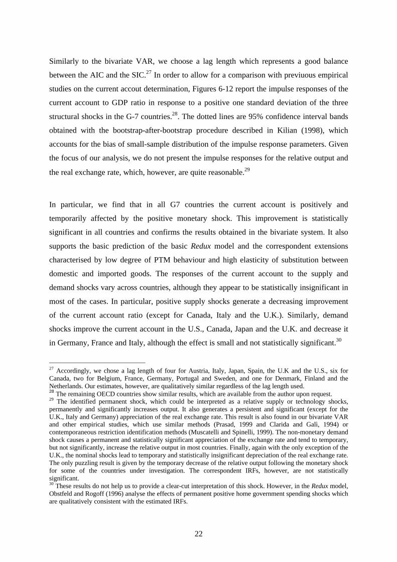
Similarly to the bivariate VAR, we choose a lag length which represents a good balance
between the AIC and the SIC.27 In order to allow for a comparison with previuous empirical
studies on the current accout determination, Figures 6-12 report the impulse responses of the
current account to GDP ratio in response to a positive one standard deviation of the three
structural shocks in the G-7 countries.28. The dotted lines are 95% confidence interval bands
obtained with the bootstrap-after-bootstrap procedure described in Kilian (1998), which
accounts for the bias of small-sample distribution of the impulse response parameters. Given
the focus of our analysis, we do not present the impulse responses for the relative output and
the real exchange rate, which, however, are quite reasonable.29
In particular, we find that in all G7 countries the current account is positively and
temporarily affected by the positive monetary shock. This improvement is statistically
significant in all countries and confirms the results obtained in the bivariate system. It also
supports the basic prediction of the basic Redux model and the correspondent extensions
characterised by low degree of PTM behaviour and high elasticity of substitution between
domestic and imported goods. The responses of the current account to the supply and
demand shocks vary across countries, although they appear to be statistically insignificant in
most of the cases. In particular, positive supply shocks generate a decreasing improvement
of the current account ratio (except for Canada, Italy and the U.K.). Similarly, demand
shocks improve the current account in the U.S., Canada, Japan and the U.K. and decrease it
in Germany, France and Italy, although the effect is small and not statistically significant.30
27 Accordingly, we chose a lag length of four for Austria, Italy, Japan, Spain, the U.K and the U.S., six forCanada, two for Belgium, France, Germany, Portugal and Sweden, and one for Denmark, Finland and theNetherlands. Our estimates, however, are qualitatively similar regardless of the lag length used.28 The remaining OECD countries show similar results, which are available from the author upon request.29 The identified permanent shock, which could be interpreted as a relative supply or technology shocks,permanently and significantly increases output. It also generates a persistent and significant (except for theU.K., Italy and Germany) appreciation of the real exchange rate. This result is also found in our bivariate VARand other empirical studies, which use similar methods (Prasad, 1999 and Clarida and Galì, 1994) orcontemporaneous restriction identification methods (Muscatelli and Spinelli, 1999). The non-monetary demandshock causes a permanent and statistically significant appreciation of the exchange rate and tend to temporary,but not significantly, increase the relative output in most countries. Finally, again with the only exception of theU.K., the nominal shocks lead to temporary and statistically insignificant depreciation of the real exchange rate.The only puzzling result is given by the temporary decrease of the relative output following the monetary shockfor some of the countries under investigation. The correspondent IRFs, however, are not statisticallysignificant.30 These results do not help us to provide a clear-cut interpretation of this shock. However, in the Redux model,Obstfeld and Rogoff (1996) analyse the effects of permanent positive home government spending shocks whichare qualitatively consistent with the estimated IRFs.

23
Table 5 shows the variance decomposition of the current account. We can easily notice the
new system confirms the quantitative importance of the monetary shock. In fact, apart from
France, Germany and the U.S. where the supply shock is dominant,31 nominal disturbances
still account for more than 50 per cent in Canada, Italy, Japan and the U.K. over the 24
period horizon. The results (not shown) for the remaining 15 OECD economies are even
more supportive, in that the monetary shock dominate the variance decomposition of the
current account (40-80 %). Differently from the bivariate specification, the demand shocks
dominate the forecast error variance decomposition of the real exchange rate. The only
exceptions are Japan and the U.S., where supply and nominal shock, respectively, provide
the major contribution. Not surprisingly, these final results suggest that the relative
importance of these shocks might be sensitive to different specifications. However, both
systems predict a significant role of nominal shocks in the current account fluctuations for a
number of OECD countries. Moreover, the estimated IRFs show that in almost all countries
a positive monetary shock generates a temporary and statistically significant current account
surplus. Both results support the empirical relevance of the basic monetary interterporal
Redux model.
Degree of openness and current account fluctuations
In this Section, we focus on an additional prediction of the OR model which refers to
relationship between country size and current account effects of monetary shocks. In
particular, by focusing on the two final equations (2.15) and (2.17) of the basic framework, it
can be seen that the larger (smaller) the home country – that is, the greater (the smaller) n –
the less (the more) the positive impact of a home money increase on its current account
(Obstfeld and Rogoff, 1995, page 643). As a result, we can expect that smaller and more
open countries will show relatively greater effects of monetary shocks on the current
account. Table 1 provides two often used indicators of openness to international trade: the
31 In the U.S. case, Lane (1999) provides similar results and shows that the identified monetary shock accountsfor about 50% of the variance of the current account. His specification, however, does not provide similarresults for the other countries. In particular, we have estimated the same trivariate VAR system (i.e. relativeoutput, the ratio of current account to output and relative prices) and imposed the same long-run restrictions forthe G7 over our sample period. Results are much less clear-cut in that, while the IRFs are qualitatively similarto ours, they are not statistically significant. Moreover, with the only exception of the U.S., the size of thecontribution of monetary shocks in current account fluctuations is less important (i.e. between 5-10 per cent

24
ratio of total exports to real GDP and the ratio of total trade volumes to real GDP. Figures
refer to average values over the period 1980-1998 GDP for the 15 OECD countries. From
the two columns, it is evident that the two ratios provide the same classification. In
particular, as expected, relatively smaller countries seem to be more open, whereas low
values of the indicators are associated with relatively larger countries.
In order to test formally for this prediction, we standardise the maximum effect of the
estimated current account impulse response to the identified monetary policy shock
according for all the countries. Figure 2 plots this criterion against the ratio of the overall
trade to real GDP. Although the specific proxy for the trade openness and the imprecise
estimates of the impulse responses might bias such an exercise, the upward fitted line clearly
shows a positive correlation. This result supports the theoretical prediction from above, and
might be interpreted as an additional positive result demonstrating the consistency of the
VAR system and the theory.
TABLE 1 Measures of Openness
Overall exports as% GDP
Overall exportsplus imports as %
GDPAustria 37.1 74.0Belgium 68.5 134.6Canada 27.5 54.1Denmark 33.9 65.2Finland 28.8 56.2France 22.0 43.4Germany 26.5 50.8Italy 19.9 39.9Netherlands 11.4 100.6Portugal 30.6 69.1Spain 19.2 39.4Sweden 32.2 62.5United Kingdom 25.6 52.2United States 9.0 19.3
Sources: our estimates on OECD data.
over six years forecast horizon). These results might depend on the fact that a statistically incorrect long-runrestriction is imposed on the current account to GDP ratio, which is stationary in our sample period.

25
CHART 1 Openness and current account effects to MS
Source: our estimates
30
40
50
60
70
80
90
100
0 50 100 150

26
7. Conclusions
The intertemporal approach to the current account has been of fundamental importance in
explaining current account imbalances. However, most of the literature has focused on
productivity and fiscal shocks as main determinants of its variations. In this paper, we
emphasise the importance of nominal (or monetary) shocks in generating exchange rate and
current account fluctuations, by first outlining the standard monetary version (and some
closely related extensions) of the sticky price intertemporal model of Obstfeld and Rogoff
(1995, 1996), and then empirically investigating the main predictions of this class of models.
We use two structural VAR models to estimate the responses to real and nominal shocks
across 15 OECD countries over the period 1979Q1 to 1998Q4. Similarly to Blanchard and
Quah (1989), we achieve identification of the model by imposing long-run restrictions and
leaving the short run fluctuations of the variables to be determined by the data. The forecast
error variance decomposition shows strong evidence in favour of a crucial role of monetary
shocks in generating current account movements in most of the countries. Moreover, the
estimated impulse response functions to the identified monetary shock are very much in line
with the main predictions of the Obstfeld and Rogoff model, in which unexpected monetary
policy shocks temporarily and significantly improve the current account. Our results provide
strong support in favour of the basic Redux model, and weak empirical evidence of those
extensions of the basic framework – introduction of high degree of PTM behaviour (Betts
and Devereux, 2000) and poor elasticity of substitution between domestic and imported
goods (Tille, 2001)- in which a current account neutrality or deficit is predicted.
In the last Section we have verified a further prediction of this class of models. In particular,
we have shown that trade openness of the country, which is strictly dependent on the size of
the 15 economies under investigation, is positively correlated with the estimated maximum
effect of the current account to the identified monetary shock.

27
Bibliography
Bayoumy, T. and B. Eichengreen (1992), “Shocking aspects of European monetaryintegration”, CEPR Discussion Paper, no. 643 and in Torres F. and F. Giavazzi (1993), eds.,“Adjustments and Growth in the European Monetary Union,” Cambridge University Press,pp. 193-240.
Betts, C. and M. Devereux (1996), “The exchange rate in a model of pricing-to-market,”European Economic Review, Vol. 40, pp. 1007-1021.
Betts, C. and M. Devereux (1999), “The International Effects of Monetary and FiscalPolicy in a Two-Country Model,” mimeo, University of British Columbia.
Betts, C. and M. Devereux (2000), “Exchange Rate Dynamics in a Model of Pricing toMarket,” Journal of International Economics, Vol. 50, pp. 215-44.
Blanchard, O. J. and N. Kiyotaki (1987), “Monopolistic Competition and the Effects ofAggregate Demand,” American Economic Review, Vol. 77, no. 4, September, pp. 647-666.
Blanchard, O. J. and D. Quah (1989), “The Dynamic Effects of Aggregate Demand andSupply Disturbances,” American Economic Review, Vol. 79, September, pp. 655-673.
Cavallari, L. (2001), “Current Account and Exchange Rate Dynamics,” Economic Notes,Vol. 30, no. 1.
Chari, V.V., P.J. Kehoe and E.R. McGrattan (1997), “Monetary Shocks and the RealExchange Rates in Sticky Price Models of International Business Cycles,” NBER WorkingPaper, no. 5876.
Clarida, R. and J. Galì (1994), “Sources Of real exchange-rate fluctuations: Howimportant are nominal shocks?," Carnegie-Rochester Conference Series on Public Policy,no. 41, pp. 1-56.
Devereux, M. (1999), “How Does a Devaluation Affect the Current Account?,” DiscussionPaper, Department of Economics, University of British Columbia, no. 99-08.
Eichenbaum, M. and C. Evans (1995), “Some Empirical Evidence on the Effects of Shocksto Monetary Policy on Exchange Rates,” Quarterly Journal of Economics, Vol. 110, pp. 975-1010.
Engel, C. (1993), “Real Exchange Rates and Relative Prices: an Empirical Investigation,”Journal of Monetary Economics, Vol. 32, pp. 35-50.
Engel, C. and J.H. Rogers (1996), “How wide is the border?,” American EconomicReview, Vol. 77, pp. 93-106.

28
Erkel-Rousse, H. and J. Melitz (1994), “New Empirical Evidence on the Costs ofEuropean Monetary Union,” CEPR Working Paper, no. 1169 and in Eijffinger S. and H.Huizinga (1996), eds., “Positive Political Economy: Theory and Evidence,” CambridgeUniversity Press.
Fanke, M. (2000), “Macroeconomic Shocks in Euroland vs. the U.K.: Supply, Demand, orNominal?, Hamburg University, mimeo.
Froot, K.A. and K. Rogoff (1995), “Perspectives on PPP and long-run exchange rates,”NBER Working Paper, no. 4952.
Galí, J. (1992), “How well does the IS-LM model fit post-war U.S. data?,”Quarterly Journalof Economics, Vol. 107, pp. 709-38.
Glick, R. and K. Rogoff (1995), "Global versus country-specific productivity shocks andthe current account," Journal of Monetary Economics, Vol. 35, pp. 159-92.
Kollmann, R. (1997), "The Exchange Rate in a Dynamic-Optimising Current AccountModel with Nominal Rigidities: A Quantitative Investigation," IMF Working Paper, 97/7,January.
Kaminsky, G. and M. Klein (1994), “The real exchange rate and fiscal policy during thegold standard period: evidence from the United States and Great Britain,” NBER WorkingPaper, no. 4809.
Kilian, L. (1998), “Small Sample Confidence Intervals for Impulse Response Functions”,Reviw of Economics and Statistics, pp. 218-230.
Kim, S. (1999), “Do monetary policy shocks matter in the G-7 countries? Using commonidentifying assumptions about monetary policy across countries”, Journal if InternationalEconomics, Vol. 48, pp. 387-412.
Kwiatkowsky D., P. C. B. Phillips, P. Schmidt and Y. Shin (1992), "Testing the nullhypothesis of stationarity against the alternative of unit root," Journal of Econometrics, Vol.54, pp. 159-178.
Lane, P.R. (1999), “Money Shocks and the Current Account,” in Calvo G., R. Dornbushand M. Obstfeld, eds, “Money, Factor Mobility and Trade: Essays on Honor of RobertMundell,” MIT Press, Cambridge.
Lane, P.R. (2001), “The New Open Economy Macroeconomics: A Survey,” Journal ofInternational Economics, Vol. 54, page 235-266.
Lane, P.R. and G.M. Milesi-Ferretti (2000), “The Transfer Problem Revisited: NetForeign Assets and Real Exchange Rates”, mimeo.
Lee, J. and M. Chinn (1998), “The Current Account and the Real Exchange Rate: AStructural VAR Analysis of Major Currency,” NBER Working Paper, no. 6495.

29
Lombardo, G. (2001), “On the trade balance response to monetary shocks: the Marshall-Lerner conditions reconsidered,” Department of Economics, Trinity College, Dublin,mimeo.
Melitz, J. and A. Weber (1996), “The Costs/Benefits of a Common Monetary Policy inFrance and Germany and Possible Lessons for Monetary Union,” CEPR Discussion Paper,no. 1374, April.
Obstfeld, M. and K. Rogoff (1995), “Exchange Rate Dynamics Redux,” Journal of PoliticalEconomy, Vol. 103, no. 3, June, pp. 624-660.
Obstfeld, M. and K. Rogoff (1995a), “The Intertemporal Approach to the CurrentAccount,” in G. Grossman and K. Rogoff, eds., Handbook of International Economics, Vol.3, Amsterdam: North Holland.
Obstfeld, M. and K. Rogoff (1996), “Foundations of International Macroeconomics,”Cambridge, MA: MIT Press.
Obstfeld, M. and K. Rogoff (1999), “New Directions for Stochastic Open EconomyModels,” NBER Working Paper, no. 7313.
Prasad, E. S. (1999), "International Trade and the Business Cycle," Economic Journal, Vol.109, no. 458, pp. 588-606.
Prasad, E. S. and J.A. Gable (1998), "International Evidence on the Determinants of TradeDynamics," IMF Staff Papers, Vol. 45, no. 3, pp. 401-39.
Rogoff, K. (1992), “Trade goods consumption smoothing and the random walk behaviour ofthe real exchange rate,” Bank of Japan Monetary and Economic Studies, Vol. 10, pp. 1-29.
Rogoff, K. (1995), “The Purchasing Power Parity Puzzle,” Journal of Economic Literature,Vol. 34, pp. 647-668, June.
Sims, C. A. (1992), “Interpreting the Macroeconomic Time Series Facts. The Effects ofMonetary Policy,” European Economic Review, Vol. 36, pp. 975-1011.
Tille, C. (2001), “The Role of Consumption Substitutability in the IntertemporalTransmission of Monetary Shocks," Journal of International Economics, Vol. 53, pp. 421-44.
Walsh, C. E. (1998), “Monetary Theory and Policy,” The MIT Press, London, 1998.

30
APPENDIX 1 – Data Description and Unit Root Analysis
As in Lee and Chinn (1998), in the first bivariate system we use the CPI-deflated real
exchange rate, the nominal current account in US dollars, and the national-currency
denominated GDP in nominal terms data taken from the International Financial Statistics
(IFS) published by the International Monetary Fund.32 Additionally, for the second
specification, we take seasonally adjusted GDP data denominated in national currency taken
from the same source. In our estimations, we use the log of the real exchange rate (REER),
the ratio of the current account to GDP (CA/Y), and the log ratio of real domestic GDP to
foreign real GDP (Y/Y*).
The original current account series are in US dollars and non-seasonally adjusted. Following
Lee and Chinn (1998), we obtain the national currency-denominated current account, by
using the average bilateral exchange rate of each period. We then calculate the ratio CA/Y,
and seasonally adjust them using dummy variables. For the G7 countries, the rest of the
world (or foreign) real GDP for each country is proxied and constructed as the trade-
weighted sum of US$-denominated real GDP of the remaining G7.
For most of the countries, the data are over 1979:1-1999:4 (1979:1-1998:4 in the three-
variable system). The only exceptions are Belgium and Denmark, in which data are only
available after 1985:1 and 1987:1, respectively.
Testing for Unit Roots
Tables 1, 2 and 3 tabulate the unit root test results for all of the series. Column 1 shows the
ADF test statistics. Column 2 provides the optimum lag length, which has been selected on
the basis of the significance of the coefficients of the lagged terms, and the white noise
properties of the residuals33. In the third column, we indicate the deterministic components
in the regression model used for testing. Alternative deterministic term combinations have
been tested in order to reinforce the reported results. In the last column, we show the critical
values at the 1% and 5% level of significance provided by MacKinnon (1991).
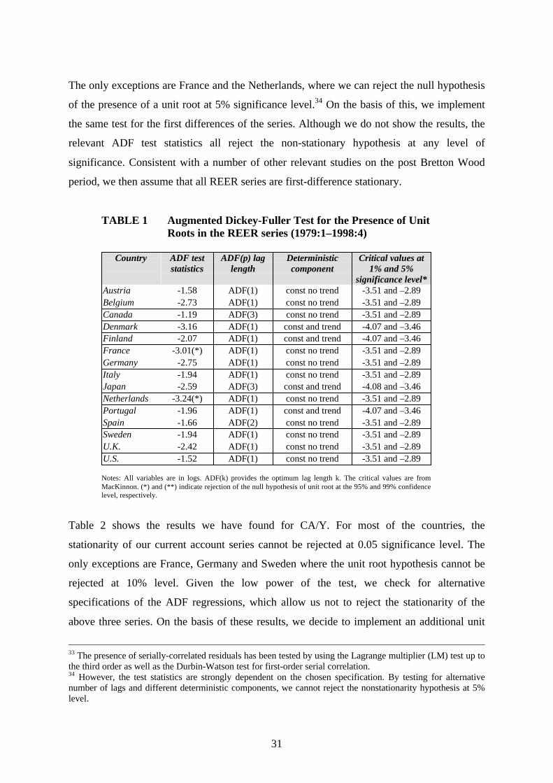
As far as the REER series is concerned, the results suggest that we cannot reject the null
hypothesis of non-stationarity indicating that all the variables are not stationary in levels.
32 It is worth pointing out that, according to the Fund's definition and construction of the index, a decrease inthe real effective exchange rate reflects a depreciation.
31
The only exceptions are France and the Netherlands, where we can reject the null hypothesis
of the presence of a unit root at 5% significance level.34 On the basis of this, we implement
the same test for the first differences of the series. Although we do not show the results, the
relevant ADF test statistics all reject the non-stationary hypothesis at any level of
significance. Consistent with a number of other relevant studies on the post Bretton Wood
period, we then assume that all REER series are first-difference stationary.
TABLE 1 Augmented Dickey-Fuller Test for the Presence of UnitRoots in the REER series (1979:1–1998:4)
Country ADF teststatistics
ADF(p) laglength
Deterministiccomponent
Critical values at1% and 5%
significance level*Austria -1.58 ADF(1) const no trend -3.51 and –2.89Belgium -2.73 ADF(1) const no trend -3.51 and –2.89Canada -1.19 ADF(3) const no trend -3.51 and –2.89Denmark -3.16 ADF(1) const and trend -4.07 and –3.46Finland -2.07 ADF(1) const and trend -4.07 and –3.46France -3.01(*) ADF(1) const no trend -3.51 and –2.89Germany -2.75 ADF(1) const no trend -3.51 and –2.89Italy -1.94 ADF(1) const no trend -3.51 and –2.89Japan -2.59 ADF(3) const and trend -4.08 and –3.46Netherlands -3.24(*) ADF(1) const no trend -3.51 and –2.89Portugal -1.96 ADF(1) const and trend -4.07 and –3.46Spain -1.66 ADF(2) const no trend -3.51 and –2.89Sweden -1.94 ADF(1) const no trend -3.51 and –2.89U.K. -2.42 ADF(1) const no trend -3.51 and –2.89U.S. -1.52 ADF(1) const no trend -3.51 and –2.89
Notes: All variables are in logs. ADF(k) provides the optimum lag length k. The critical values are fromMacKinnon. (*) and (**) indicate rejection of the null hypothesis of unit root at the 95% and 99% confidencelevel, respectively.
Table 2 shows the results we have found for CA/Y. For most of the countries, the
stationarity of our current account series cannot be rejected at 0.05 significance level. The
only exceptions are France, Germany and Sweden where the unit root hypothesis cannot be
rejected at 10% level. Given the low power of the test, we check for alternative
specifications of the ADF regressions, which allow us not to reject the stationarity of the
above three series. On the basis of these results, we decide to implement an additional unit
33 The presence of serially-correlated residuals has been tested by using the Lagrange multiplier (LM) test up tothe third order as well as the Durbin-Watson test for first-order serial correlation.34 However, the test statistics are strongly dependent on the chosen specification. By testing for alternativenumber of lags and different deterministic components, we cannot reject the nonstationarity hypothesis at 5%level.

32
root test, that is, the KPSS test. Our results (not shown) are again supportive of the
hypothesis of stationarity of the series.35
TABLE 2 Augmented Dickey-Fuller Test for the Presence ofUnit Roots in the CA/Y series (1979:1–1998:4)
Country ADF teststatistics
ADF(p) laglength
Deterministiccomponent
Critical values at1% and 5%
significance level*Austria -3.85(**) ADF(0) no const no trend -2.59 and –1.94Belgium -5.68(**) ADF(0) const and trend -4.13 and –3.59Canada -2.96(**) ADF(0) no const no trend -2.59 and –1.94Denmark -2.09(*) ADF(3) no const no trend -2.61 and –1.94Finland -2.06(*) ADF(0) no const no trend -2.59 and –1.94France -3.16 ADF(1) const and trend -4.08 and –3.46Germany -1.86 ADF(1) no const no trend -2.59 and –1.94Italy -2.48(*) ADF(0) no const no trend -2.59 and –1.94Japan -2.35(*) ADF(0) no const no trend -2.59 and –1.94Netherlands -2.02(*) ADF(2) no const no trend -2.59 and –1.94Portugal -2.00(*) ADF(1) no const and trend -2.59 and –1.94Spain -2.14(*) ADF(2) no const and trend -2.59 and –1.94Sweden -1.83 ADF(1) no const no trend -2.59 and –1.94U.K. -1.95(*) ADF(1) no const no trend -2.59 and –1.94U.S. -2.17(*) ADF(6) no const no trend -2.59 and –1.94
Notes: All variables are in logs. ADF (k) provides the optimum lag length k. the critical values are fromMacKinnon. (*) and (**) indicate rejection of the null hypothesis of unit root at the 95% and 99% confidencelevel, respectively.
Finally, Table 3 provides the results for the relative output variable Y/Y*. For all countries,
we cannot reject the null hypothesis of non-stationarity at any level of significance. By
implementing the same test for the first differences of the series (results not shown), the
relevant ADF test statistics all reject the non-stationary hypothesis. Therefore, we conclude
that the relative output Y/Y* is non-stationary in levels, and stationary in first differences.
35 These results are consistent with the stationarity test on the same variable for the G-7 countries implementedby Lee and Chinn (1998). In their paper, they use the KPSS test and find that, for most countries, thestationarity of the current account series cannot be rejected at 5% level.

33
TABLE 3 Augmented Dickey-Fuller Test for the Presence ofUnit Roots in the Y/Y* series (1979:1–1998:4)
Country ADF teststatistics
ADF(p) laglength
Deterministiccomponent
Critical values at1% and 5%
significance levelAustria -2.12 ADF(4) const no trend -3.51 and –2.89Belgium -2.06 ADF(1) const no trend -3.51 and –2.89Canada -0.79 ADF(1) const and trend -4.08 and –3.46Denmark -3.21(*) ADF(1) const no trend -3.51 and –2.89Finland -1.38 ADF(1) const no trend -3.51 and –2.89France -2.34 ADF(1) const no trend -3.51 and –2.89Germany -1.96 ADF(1) const and trend -4.07 and –3.46Italy -2.09 ADF(1) const and trend -4.07 and –3.46Japan -1.53 ADF(1) no const no trend -2.59 and –1.94Netherlands -2.51 ADF(1) const and trend -4.07 and –3.46Portugal -1.85 ADF(1) const no trend -3.51 and –2.89Spain -2.67 ADF(1) const no trend -3.51 and –2.89Sweden -2.24 ADF(1) const and trend -4.07 and –3.46U.K. -2.14 ADF(1) const no trend -3.51 and –2.89U.S. -0.49 ADF(3) no const no trend -2.59 and –1.94
Notes: All variables are in logs. ADF(k) provides the optimum lag length k. The criticalvalues are from MacKinnon. (*) and (**) indicate rejection of the null hypothesis ofunit root at the 95% and 99% confidence level, respectively.

34
FIGURE 2 Impulse Responses for France. Bivariate VAR
FIGURE 3 Impulse Responses for Spain. Bivariate VAR
Temp. Shock to CA
-0.005
0
0.005
0.01
0.015
1 3 5 7 9 1 1 1 3 1 5 1 7 1 9 2 1 2 3 2 5
Temp. Shock to RER
-0.04-0.03-0.02-0.01
00.01
1 3 5 7 9 1 1 1 3 1 5 1 7 1 9 2 1 2 3 2 5
Perm. Shock to RER
00.010.020.030.040.050.06
1 3 5 7 9 1 1 1 3 1 5 1 7 1 9 2 1 2 3 2 5
Perm. Shock to CA
-0.005
0
0.005
0.01
0.015
1 3 5 7 9 1 1 1 3 1 5 1 7 1 9 2 1 2 3 2 5
Temp. Shock to RER
-0.025-0.02
-0.015-0.01
-0.0050
0.0050.01
1 3 5 7 9 1 1 1 3 1 5 1 7 1 9 2 1 2 3 2 5
Temp. Shock to CA
0
0.002
0.004
0.006
0.008
1 3 5 7 9 1 1 1 3 1 5 1 7 1 9 2 1 2 3 2 5
Perm. Shock to CA
-0.004-0.002
00.0020.0040.0060.008
0.01
1 3 5 7 9 1 1 1 3 1 5 1 7 1 9 2 1 2 3 2 5
Perm. Shock to RER
-0.010
0.010.020.030.04
1 3 5 7 9 1 1 1 3 1 5 1 7 1 9 2 1 2 3 2 5

35
FIGURE 4 Impulse Responses for Sweden. Bivariate VAR
FIGURE 5 Impulse Responses for the U.S.. Bivariate VAR
Temp. Shock to CA
-0.002-0.001
00.0010.0020.0030.004
1 3 5 7 9 1 1 1 3 1 5 1 7 1 9 2 1 2 3 2 5
Temp. Shock to RER
-0.05-0.04-0.03-0.02-0.01
00.01
1 3 5 7 9 1 1 1 3 1 5 1 7 1 9 2 1 2 3 2 5
Perm. Shock to RER
-0.020
0.020.040.060.08
0.1
1 3 5 7 9 1 1 1 3 1 5 1 7 1 9 2 1 2 3 2 5
Perm. Shock to CA
-0.0010
0.0010.0020.0030.0040.0050.006
1 3 5 7 9 1 1 1 3 1 5 1 7 1 9 2 1 2 3 2 5
Perm. Shock to CA
-0.01-0.005
00.005
0.010.015
0.02
1 3 5 7 9 1 1 1 3 1 5 1 7 1 9 2 1 2 3 2 5
Perm. Shock to RER
00.010.020.030.040.050.06
1 3 5 7 9 1 1 1 3 1 5 1 7 1 9 2 1 2 3 2 5
Temp. Shock to CA
0
0.005
0.01
0.015
0.02
1 3 5 7 9 1 1 1 3 1 5 1 7 1 9 2 1 2 3 2 5
Temp. Shock to RER
-0.04-0.03-0.02-0.01
00.010.02
1 3 5 7 9 1 1 1 3 1 5 1 7 1 9 2 1 2 3 2 5

36
TABLE 4 Variance Decomposition of Current Account. Bivariate VAR.
FRANCE
0%
20%
40%
60%
80%
100%
1 3 5 7 9 11 13 15 17 19 21 23
Permanent Shock Temporary Shock
SPAI N
0%
20%
40%
60%
80%
100%
1 3 5 7 9 11 13 15 17 19 21 23
Permanent Shock Temporary Shock
SWEDEN
0%
20%
40%
60%
80%
100%
1 3 5 7 9 11 13 15 17 19 21 23
Permanent Shock Temporary Shock
U. S.
0%
20%
40%
60%
80%
100%
1 3 5 7 9 11 13 15 17 19 21 23
Permanent Shock Temporary Shock

37
FIGURE 6 Response of CA to Structural Shocks for Canada. Trivariate VAR.
Monetary Shock
Demand Shock
Supply Shock
-0.004
-0.002
0
0.0020.004
0.006
0.008
0.01
1 3 5 7 9 1 1 1 3 1 5 1 7 1 9 2 1 2 3 2 5
-0.006-0.004-0.002
00.0020.0040.0060.008
0.01
1 3 5 7 9 1 1 1 3 1 5 1 7 1 9 2 1 2 3 2 5
-0.01-0.008-0.006-0.004-0.002
00.0020.0040.0060.008
0.01
1 3 5 7 9 1 1 1 3 1 5 1 7 1 9 2 1 2 3 2 5

38
FIGURE 7 Response of CA to Structural Shocks for France. Trivariate VAR
Monetary Shock
Demand Shock
Supply Shock
00.0010.0020.0030.0040.0050.0060.0070.008
1 3 5 7 9 1 1 1 3 1 5 1 7 1 9 2 1 2 3 2 5
-0.005-0.004-0.003-0.002-0.001
00.0010.0020.0030.004
1 3 5 7 9 1 1 1 3 1 5 1 7 1 9 2 1 2 3 2 5
-0.002
0
0.002
0.004
0.006
0.008
0.01
1 3 5 7 9 1 1 1 3 1 5 1 7 1 9 2 1 2 3 2 5

39
FIGURE 8 Response of CA to Structural Shocks for Germany. Trivariate VAR
Monetary Shock
Demand Shock
Supply Shock
-0.004
-0.002
0
0.0020.004
0.006
0.008
0.01
1 3 5 7 9 1 1 1 3 1 5 1 7 1 9 2 1 2 3 2 5
-0.01
-0.008
-0.006
-0.004-0.002
0
0.002
0.004
1 3 5 7 9 1 1 1 3 1 5 1 7 1 9 2 1 2 3 2 5
-0.004-0.002
00.0020.0040.0060.008
0.010.012
1 3 5 7 9 1 1 1 3 1 5 1 7 1 9 2 1 2 3 2 5
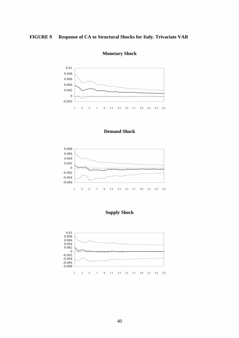
40
FIGURE 9 Response of CA to Structural Shocks for Italy. Trivariate VAR
Monetary Shock
Demand Shock
Supply Shock
-0.002
0
0.002
0.004
0.006
0.008
0.01
1 3 5 7 9 1 1 1 3 1 5 1 7 1 9 2 1 2 3 2 5
-0.006
-0.004
-0.002
00.002
0.004
0.006
0.008
1 3 5 7 9 1 1 1 3 1 5 1 7 1 9 2 1 2 3 2 5
-0.008-0.006-0.004-0.002
00.0020.0040.0060.008
0.01
1 3 5 7 9 1 1 1 3 1 5 1 7 1 9 2 1 2 3 2 5

41
FIGURE 10 Response of CA to Structural Shocks for Japan. Trivariate VAR
Monetary Shock
Demand Shock
Supply Shock
-0.002
-0.001
0
0.0010.002
0.003
0.004
0.005
1 3 5 7 9 1 1 1 3 1 5 1 7 1 9 2 1 2 3 2 5
-0.004-0.003-0.002-0.001
00.0010.0020.0030.004
1 3 5 7 9 1 1 1 3 1 5 1 7 1 9 2 1 2 3 2 5
-0.002-0.001
00.0010.0020.0030.0040.0050.006
1 3 5 7 9 1 1 1 3 1 5 1 7 1 9 2 1 2 3 2 5
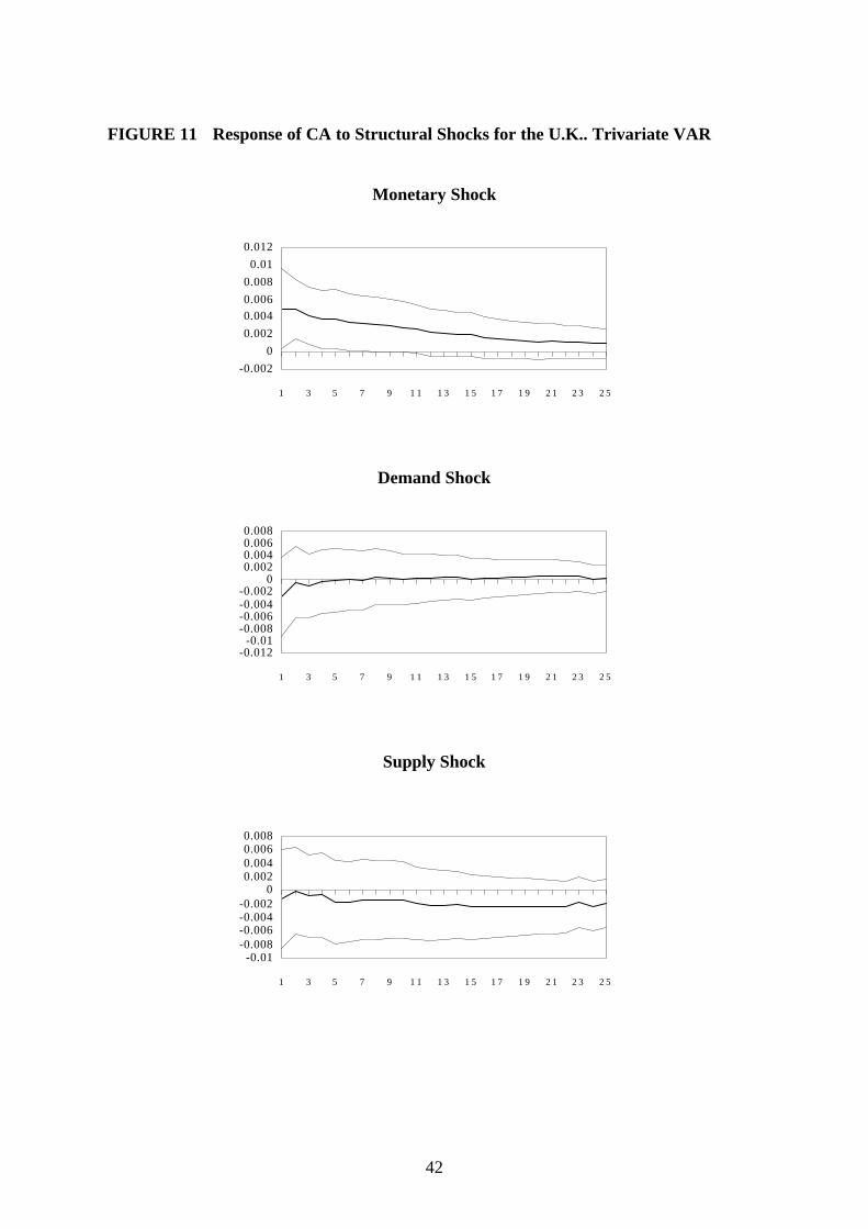
42
FIGURE 11 Response of CA to Structural Shocks for the U.K.. Trivariate VAR
Monetary Shock
Demand Shock
Supply Shock
-0.002
0
0.002
0.0040.006
0.008
0.01
0.012
1 3 5 7 9 1 1 1 3 1 5 1 7 1 9 2 1 2 3 2 5
-0.012-0.01
-0.008-0.006-0.004-0.002
00.0020.0040.0060.008
1 3 5 7 9 1 1 1 3 1 5 1 7 1 9 2 1 2 3 2 5
-0.01-0.008-0.006-0.004-0.002
00.0020.0040.0060.008
1 3 5 7 9 1 1 1 3 1 5 1 7 1 9 2 1 2 3 2 5
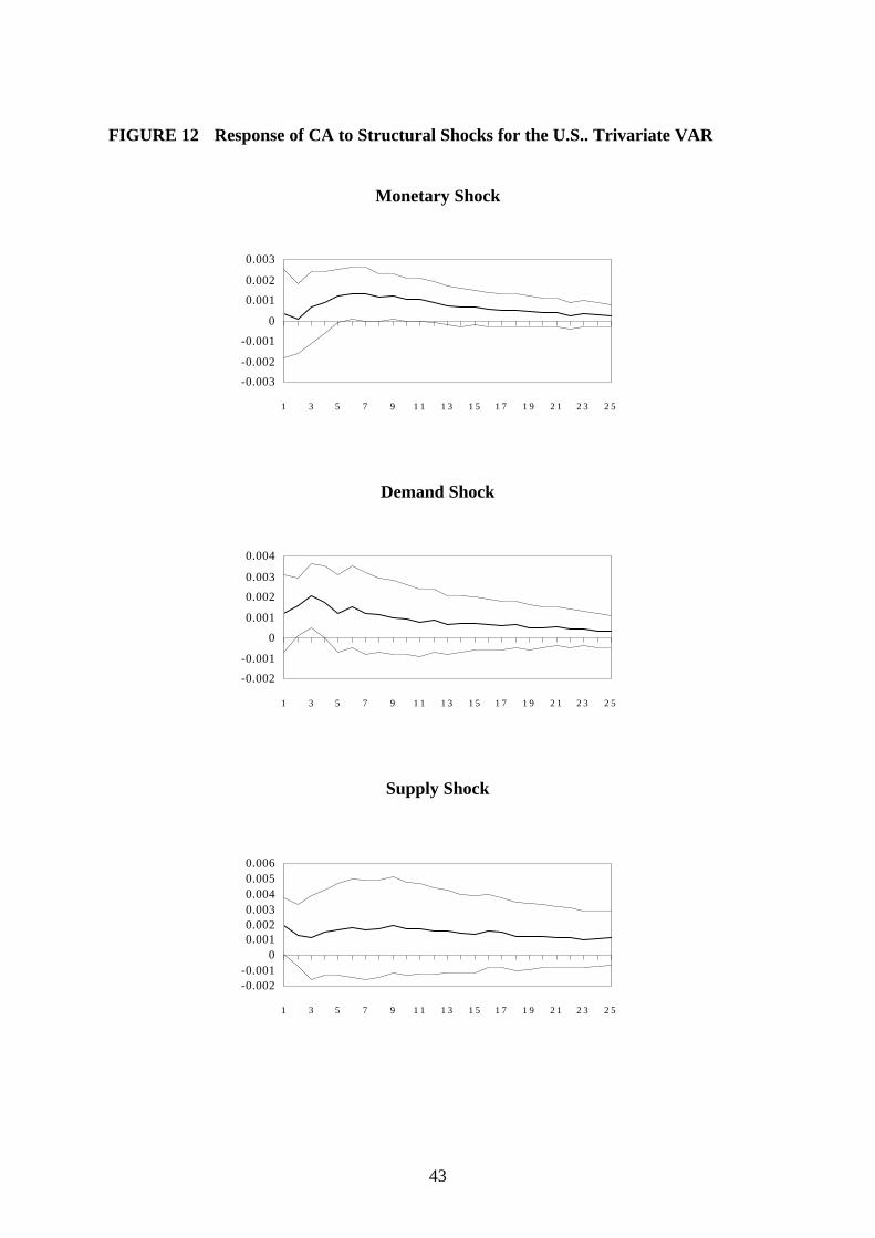
43
FIGURE 12 Response of CA to Structural Shocks for the U.S.. Trivariate VAR
Monetary Shock
Demand Shock
Supply Shock
-0.003
-0.002
-0.001
0
0.001
0.002
0.003
1 3 5 7 9 1 1 1 3 1 5 1 7 1 9 2 1 2 3 2 5
-0.002
-0.001
0
0.001
0.002
0.003
0.004
1 3 5 7 9 1 1 1 3 1 5 1 7 1 9 2 1 2 3 2 5
-0.002-0.001
00.0010.0020.0030.0040.0050.006
1 3 5 7 9 1 1 1 3 1 5 1 7 1 9 2 1 2 3 2 5

44
TABLE 4 Variance Decomposition of the Current Account. Trivariate VAR.
CANADA
0%
20%
40%
60%
80%
100%
1 3 5 7 9 11 13 15 17 19 21 23
Supply Shock Demand Shock Monetary Shock
FRANCE
0%
20%
40%
60%
80%
100%
1 3 5 7 9 11 13 15 17 19 21 23
Supply Shock Demand Shock Monetary Shock
GERMANY
0%
20%
40%
60%
80%
100%
1 3 5 7 9 11 13 15 17 19 21 23
Supply Shock Demand Shock Monetary Shock
JAPAN
0%
20%
40%
60%
80%
100%
1 3 5 7 9 11 13 15 17 19 21 23
Supply Shock Demand Shock Monetary Shock
U. K.
0%
20%
40%
60%
80%
100%
1 3 5 7 9 11 13 15 17 19 21 23
Supply Shock Demand Shock Monetary ShockU. S.
0%
20%
40%
60%
80%
100%
1 3 5 7 9 11 13 15 17 19 21 23
Supply Shock Demand Shock Monetary Shock
I TALY
0%
20%
40%
60%
80%
100%
1 3 5 7 9 11 13 15 17 19 21 23
Supply Shock Demand Shock Monetary Shock