The Empirical Content of Models with Multiple Equilibria in

Economies with Social Interactions∗

Alberto Bisin Andrea Moro Giorgio Topa†

June 27, 2011

Abstract

We study a general class of models with social interactions that might display mul-

tiple equilibria. We propose an estimation procedure for these models and evaluate

its efficiency and computational feasibility relative to different approaches taken to the

curse of dimensionality implied by the multiplicity. Using data on smoking among

teenagers, we implement the proposed estimation procedure to understand how group

interactions affect health-related choices. We find that interaction effects are strong

both at the school level and at the smaller friends-network level. Multiplicity of equilib-

ria is pervasive at the estimated parameter values, and equilibrium selection accounts for

about 15 percent of the observed smoking behavior. Counterfactuals show that student

interactions, surprisingly, reduce smoking by approximately 70 percent with respect to

the equilibrium smoking that would occur without interactions.

∗We have presented preliminary versions of this research starting in 2002. Because of such a long gestation,it’s impossible to acknowledge all who gave us comments and encouragement. We are nonetheless grateful tothem. Special thanks to Konrad Menzel, Francesca Molinari, Michela Tincani, Onur Ozgur, and Joerg Stoye.This research uses data from Add Health, a program project designed by J. Richard Udry, Peter S. Bearman,and Kathleen Mullan Harris and funded by grant P01-HD31921 from the Eunice Kennedy Shriver NationalInstitute of Child Health and Human Development, with cooperative funding from 17 other agencies. Specialacknowledgment is due Ronald R. Rindfuss and Barbara Entwisle for assistance in the original design. Nodirect support was received from grant P01-HD31921 for this analysis. Finally, we thank Chris Huckfeldt,Matt Denes, and Ging Cee Ng for exceptional research assistance.†Bisin: Department of Economics, New York University, and NBER, alberto.bisin@nyu.edu. Moro:

Department of Economics, Vanderbilt University, andrea@andreamoro.net. Topa: Research Group, FederalReserve Bank of New York, giorgio.topa@ny.frb.org. The views and opinions offered in this paper do notnecessarily reflect the position of the Federal Reserve Bank of New York or the Federal Reserve System.

1 Introduction

In this paper, we study models with multiple equilibria in economies with social interactions.

Social interactions refer to socioeconomic environments in which markets do not necessarily

mediate all of the agents’ choices. In such environments, each agent’s ability to interact

with others might depend on a network of relationships, e.g., a family, a peer group, or

more generally a socioeconomic group. Social interactions represent an important aspect of

several socioeconomic phenomena, such as crime, school performance, risky sexual behavior,

alcohol and drug consumption, smoking, and obesity, and more generally are related to

neighborhood effects, which are important determinants of economic outcomes such as

employment, the patterns of bilateral trade and economic specialization, migration, urban

agglomeration, and segregation.

Social interactions typically give rise to multiple equilibria as they induce externalities.

Consider, for example, a society of agents whose preferences for smoking are stronger the

higher the proportion of smokers in the population - in other words, agents have preferences

for conformity at the global population level. In this society, we may find equilibria where

few people smoke and equilibria where many people smoke if the dependence of agents’

preferences on the proportion of smokers in the population is strong enough. But multiple

equilibria may also arise if conformity in agents’ preferences is at the level of local reference

groups, smaller than the whole population, as in the case e.g., of peer effects. It is because of

externalities of this kind that the canonical models of social interaction, Brock and Durlauf

(2001b) and Glaeser and Scheinkman (2003), also display multiple equilibria, with either

local and/or global interactions.

We refer to economies with social interactions as “societies.” We consider a general soci-

ety with (possibly) multiple equilibria and assume the econometrician observes data realized

from one or more of the equilibria. We derive conditions for identification (in the popula-

tion) of the parameters of the society. We show that identification is no more an issue when

the model has multiple equilibria than when it has a unique equilibrium. We define the like-

lihood of the data conditionally on the equilibrium selection and introduce two estimators

of the model’s structural parameters. The first estimator is based on maximizing the likeli-

hood of the data over both the set of equilibria and the set of structural parameters. Insofar

as this estimator requires the ability to compute all of the equilibria that are consistent with

1

a given set of parameters, it might represent a daunting computational task. Therefore, we

also propose a computationally simpler two-step estimation procedure that does not require

computing all feasible equilibria, nor postulating an arbitrary equilibrium selection rule. We

describe the estimators’ properties and evaluate the efficiency and computational feasibility

of the two approaches using Monte Carlo simulations. We show, in the context of Brock

and Durlauf (2001b)’s canonical model that the two-step procedure, while less efficient, is

faster by several orders of magnitude. We also show that estimation procedures based on

the adoption of an arbitrary equilibrium selection rule can be less efficient (and are again

much slower) than our two-step procedure, which is agnostic about equilibrium selection.

We conclude that the two-step estimation procedure is particularly appropriate when the

investigator does not have information about the equilibrium selection.

Furthermore, we implement the proposed two-step estimation using data from the Na-

tional Longitudinal Study of Adolescent Health (“Add Health”), a longitudinal study of

a nationally representative sample of adolescents in grades seven to twelve in the United

States during the 1994-95 school year. In this data sample, an individual’s smoking level is

positively associated with the number of smokers within the individual’s friendship network.

The positive association holds even after controlling for individual characteristics such as

grade, race, and gender. Further, the data exhibit large variation in aggregate smoking lev-

els across schools. These facts are consistent with social interactions of significant strength

and suggest that there may be scope for different schools to be in different equilibria with

regard to smoking prevalence.

We indeed estimate the parameters of various extensions of Brock and Durlauf (2001b)’s

model. Results show widespread social interactions among students, both at the level of the

school and at the level of the individuals’ friendship networks. Our parameter estimates are

consistent with the presence of multiple equilibria in our empirical application. Simulations

of the model indicate that changes in the strength of friendship or school-wide social inter-

actions (e.g., changes in the number of friends in personal networks, or in policies aimed

at discouraging tobacco use in schools) can have highly nonlinear and sometimes counter-

intuitive effects, with the possibility of large shifts in smoking prevalence because of the

presence of multiple equilibria.

We find significant heterogeneity across schools in the magnitude of the interaction

2

effects. Simulating all equilibria in each school, we find that multiple equilibria are present

in forty out of the forty-one schools used for this exercise. Simulating students’ behavior

if all schools selected the equilibrium with the lowest smoking level, we find that selection

into a higher level of smoking equilibrium accounts for about 15 percent higher smoking,

on average. Finally, to quantify the effect of social interactions, we simulate the level of

smoking that would occur if there were no preferences for peers’ behavior. Compared to

the simulated outcome without interactions, actual smoking is 70 percent lower, on average.

Somewhat contrary to standard presumptions, this result suggests that social interactions

may have an important role in reducing, rather than increasing, smoking in adolescents.

With social interactions, comovements between an individual’s and her peers’ outcomes

may be due to peer effects but also to sorting of individuals into groups according to observed

and unobserved attributes. More generally, one needs to distinguish social interaction effects

from other correlated unobservable factors that may induce the observed comovements in

outcomes. This issue is sidestepped in this paper, to focus instead on how to explicitly treat

the multiplicity of equilibria that typically arise in these economies.1

1.1 Related Literature

The identification and estimation of models with social interactions is an active area of

research. In this context, the issue of identification has been analyzed by Manski (1993) with

regards to the linear-in-means model. Though identification generally requires stringent

conditions for this class of reduced-form linear models,2 multiplicity of equilibria is typically

not an issue. Estimates of social interactions and peer effects, in this context, have been

obtained e.g., by Calvo Armengol, Patacchini, and Zenou (2009), De Giorgi, Pellizzari, and

Redaelli (2010), Patacchini and Zenou (2011a and 2011b), and Tincani (2011).

More generally, however, when agents’ policy functions are nonlinear, multiplicities arise,

especially when social interactions take the form of strategic complementarities, as in the

1See, e.g., Ioannides and Zabel (2008) and Ioannides and Zanella (2008) for empirical studies of selectionin related contexts. A companion paper, by Bisin, Moro, and Topa (in progress), addresses the possibilityof correlated unobservables by explicitly modeling the selection of individuals into networks. Preliminaryresults indicate that sorting, while statistically significant, does not reduce by much the magnitude of theestimated social interaction effects.

2Sufficient conditions for identification in this context have been proposed by Graham and Hahn (2005),Bramoulle’, Djebbari, and Fortin (2009), Davezies, D’Haultfoeuille, and Fougere (2006), and Lee (2007),among others.

3

case of preferences for conformity with a reference group. In the canonical nonlinear model

of social interactions - Brock and Durlauf (2001b)’s binary choice model - multiple equilibria

are hard to dispel, even if interactions are only global. In this class of societies, however,

social interactions are identified under functional form assumptions on the stochastic struc-

ture of preference shocks, as well as nonparametrically (Brock and Durlauf (2007)).3 Brock

and Durlauf (2001a), Krauth (2006), and Soetevent and Kooreman (2007) extend these

results to binary choice economies of local interactions.4

Indeed, in this class of nonlinear models identification is obtained under much weaker

conditions than in the class of linear economies, typically even in the case in which only one

realization of equilibrium is observed in the data, e.g., when social interactions are global and

only the actions of agents belonging to a single population are observed. In empirical work,

however, i) either sufficient conditions which guarantee a unique equilibrium are typically

assumed, as e.g., in Glaeser, Sacerdote, and Scheinkman (1996) and Head and Mayer (2008);

ii) or else a selection mechanism is specified, as e.g., in Krauth (2006) and in Soetevent and

Kooreman (2007), who exploit the structure of Nash equilibria of supermodular games

to reduce the set of equilibria under strong assumptions on the support of the selection

mechanism, and in Nakajima (2007) who instead adopts a selection mechanism which is

implicitly determined by an adaptive learning mechanism.

Important and related work on the econometrics of multiple equilibria has also been

done in macroeconomics. Dagsvik and Jovanovic (1994) study economic fluctuations in a

model with two equilibria (high and low economic activity) in each period; they postulate a

stochastic (Markovian) equilibrium selection process over time and estimate the parameters

of this process with time-series data on economic activity. The adopted functional-form

specification allows them to derive closed-form solutions of the mapping from the set of

parameters to the set of equilibria, which helps in constructing the sample likelihood for

estimation. Imrohoroglu (1993) and Farmer and Guo (1995) estimate dynamic macroeco-

nomic models of inflation and business cycles, respectively, with a continuum of equilibria

by parametrizing equilibria with a sunspot process and recovering from data the time series

3Blume, Brock, Durlauf and Ioannides (2011) provide an excellent review of the existing literature onthe identification of models with social interactions. They discuss several examples in which the presence ofmultiple equilibria helps achieve identification.

4Krauth (2006) allows for correlated effects - that is, for correlation in the preference shocks across peers,under specific parametric assumptions.

4

of the sunspot realizations under assumptions on the properties of the process; see also

Aiyagari (1995). More recent developments of these methods are surveyed in Benhabib and

Farmer (1998). In this paper, we show that assuming a specific equilibrium selection (or

sunspot) process is not always necessary and may lead to inefficient estimates if the assumed

process is not the “true” data-generating process.

A related literature studies the issue of identification and estimation in multiple equilib-

rium models of industrial organization. It concentrates on simultaneous-move finite games

of complete information where the investigator observes only the actions played by the

agents, whereas the parameters to be estimated also affect the payoffs.5 Classic examples

include the entry game studied by Bresnahan and Reiss (1991), which has extensive appli-

cations (e.g., also in labor economics). In this class of games, the model is typically not

identified: a continuum of parameter values is consistent with the same equilibrium realiza-

tion of the strategy profile. Partial identification is possible, however, as shown by Tamer

(2003) for large classes of incomplete econometric structures.6 Others, such as Bjorn and

Vuong (1985), Bresnahan and Reiss (1991), and Bajari, Hong, and Ryan (2010), have opted

for imposing assumptions that guarantee identification. Bajari, Hong, and Ryan (2010), in

particular, have interesting results about estimation as well. The estimation procedure they

adopt requires the computation of all equilibria of the game for any element of the param-

eter set and the joint estimation of the parameters of an equilibrium selection mechanism

(in an ex ante pre-specified class), which determines the probability of a given equilibrium,

as in Dagsvik and Jovanovic (1994).

Instead, Bajari, Hong, Krainer, and Nekipelov (2006) and Aguirregabiria-Mira (2007)

study, respectively, static and dynamic versions of a discrete entry game of incomplete

information. In this context, they study the properties of a two-step estimator similar

in spirit to ours.7 A version of this estimator had been introduced by Moro (2003) in the

context of a model of statistical discrimination in the labor market.8 In that application, the

5See Berry and Tamer (2007) for a survey of this literature.6See also Manski and Tamer (2002), Andrews, Berry, and Jia (2004), Ciliberto and Tamer (2009),

Beresteanu, Molchanov, and Molinari (2008), and Galichon and Henry (2008). Echenique and Komunjer(2005) have results regarding the identification of monotone comparative statics in incomplete econometricstructures.

7See also Pakes, Ostrovsky, and Berry (2004), Pesendorfer and Schmidt-Dengler (2004), and Bajari,Benkard, and Levin (2007); see Aguirregabiria (2004) for some foundational theoretical econometric work.

8See also Fang 2006.

5

equilibrium map linking wages to the individual workers’ characteristics is different across

different equilibria, hence the model can be identified and estimated off cross-sectional data.

Finally, our application to teenagers’ smoking behavior is also specifically related to a

large empirical literature. These studies generally document strong social interactions, or

peer effects, in smoking decisions. However part of the literature relies on linear-in-means

models which, as shown by Manski (1993), are not identified. As a result, it tends to

attribute to social interactions any effects that are possibly due instead to selection and/or

common shocks. This is the case, e.g., of Wang, Fitzhugh, Westerfield, and Eddy (1995)

and Wang, Eddy, and Fitzhugh (2000); see also the review in Tyas and Pederson (1998).

Instrumental variable estimates, as in Norton, Lindrooth, and Ennett (1998), Gaviria and

Raphael (2001), and Powell, Tauras, and Ross (2003), attempt to address these problems.9

The evidence for strong social interactions in smoking is maintained when non-linear models

are estimated which are better identified, e.g., by Krauth (2006), Soetevent and Kooreman

(2007), and Nakajima (2007).

2 A general society

Consider a society populated by a set of agents indexed by i ∈ I. The population is par-

titioned into sub-populations indexed by n = 1, ..., N and represented by disjoint sets In

such thatN⋃n=1

In = I. Let |In| denote the dimensionality of set In and |I| the dimensionality

of I. We shall be interested in the limit where each sub-population n is composed of count-

ably infinite agents. Different sub-populations can be interpreted as neighborhoods, ethnic

groups, schools, etc.

Network. The network structure of the society is characterized by a map g from the set

of agents I to its power set P, so that g(i) ⊂ I denotes the group of agents in the society

that interact with agent i. We assume each agent i ∈ In interacts locally with a finite

group g(i) ⊂ In, composed of members of her own sub-population.10 Let | g(i) |<∞ be the

dimensionality of g(i).

Exogenous characteristics. Each agent i ∈ I is characterized by a vector of exogenous

9See also Bauman and Fisher (1986), Krosnick and Judd (1982), and Jones (1994).10This is not a restriction on but rather a definition of the concept of sub-population. Also, we construct

the network so that g(i) does not contain i.

6

characteristics xi ∈ X. Each sub-population n is in turn characterized by a vector of

exogenous characteristics zn ∈ Z. Let z = (zn)n∈N , xn = (xi)i∈In , and x = (xi)i∈I . We

assume X and Z are compact sets.

Actions. Each agent i ∈ I chooses an element yi in a compact set Y (possibly a discrete

set). Agents’ choices are simultaneous. Let yg(i), yn, denote the vectors of choices in groups

g(i) and In, respectively, and let y denote the vector of choices of all agents.

Uncertainty. Let εi denote a vector of idiosyncratic shocks hitting agent i ∈ I; let un

denote the vector of aggregate shocks hitting all agents i ∈ In, and let u = (un)n∈N . All

shocks are defined on a compact support.11 For any i ∈ In let p(εi | zn, un) denote the

conditional probability of the shocks εi. We allow the distribution p(εi | zn, un) to depend

on the choice vector yn. We assume εi and εj are conditionally independent across i, j ∈ In,

for any n ∈ N . Let p(u) denote the probability of u. Typically, these shocks are preference

shocks, but they could also represent technology shocks.

Global interactions. Let πn denote an A-dimensional vector of equilibrium aggregates

defined at the level of sub-population n. Typically, πn contains an externality, a global

social interaction effect. If the society has a competitive market component, then πn would

typically also contain the vector of competitive equilibrium prices. Let A denote an (A-

dimensional) vector valued continuous map A (yi, xi, πn, zn, un) such that equilibrium con-

ditions in sub-population n are written

lim|In|→∞

1

|In|∑i∈In

A (yi, xi, πn, zn, un) = 0

The map A could have a component Aj representing, e.g., the excess demand for

commodity j of agent i with characteristics xi in a sub-population n characterized by

(πn, zn, un). The condition lim|In|→∞1|In|∑

i∈In Aj (yi, xi, πn, zn, un) = 0 would in this case

represent market clearing for commodity j in sub-population n. Also, the map A could have

a componentAj′ such that lim|In|→∞1|In|∑

i∈In Aj′ (yi, xi, πn, zn, un) = lim|In|→∞1|In|∑

i∈In yi−

πn, so that πn represents the average action in sub-population n (if Y = {0, 1} then πn

represents the fraction of agents in sub-population n choosing an element of y = 1).12

11To simplify notation, we avoid specifying formally the probability spaces on which random variables aredefined. We also refer generally to probability functions, which are to be interpreted as density functionswhen the underlying space is continuous.

12 We implicitly require that both externalities and markets do not extend across the sub-population, as

7

Choice. Any agent i ∈ I, before choosing yi observes the private shocks, the realization

un, the whole vector xn, and zn.13 We shall also assume that the maximization problem of

each agent is sufficiently regular for equilibrium conditions to be well-behaved mathemat-

ical objects amenable to standard calculus techniques. Detailed assumptions and formal

arguments are relegated to Appendix A.14

The set of first-order conditions that determine the choice of an arbitrary agent i ∈ Ininduces a conditional probability distribution on (y, x), Pi

(y, x | yg(i), πn, zn, un

).15

2.1 Equilibrium

At equilibrium in sub-population n, the first-order conditions are satisfied jointly for any

agent i ∈ In and the equilibrium aggregates πn satisfy a set of consistency and market-

clearing conditions. Formally:

Definition 1 An equilibrium in society, given (zn, un) for any n ∈ N , is represented

by a probability distribution on the configuration of actions and characteristics (yn,xn),

P (yn,xn | zn, un), and an A−dimensional vector πn such that:

1. P (yn,xn | zn, un) is ergodic and satisfies

P(yi = y, xi = x | yg(i), zn, un

)= Pi

(y, x | yg(i), πn, zn, un

), P − a.s., (1)

for any i ∈ In and any (x, y) ∈ X × Y ;

2. πn satisfies

EP [A (yi, xi, πn, zn, un)] = 0, for any i ∈ In. (2)

where the expectation is taken with respect to P (yn,xn | zn, un).

no πn′ , n′ 6= n, enters in the equilibrium condition for sub-population n. In fact, our analysis is unchanged ifwe allow for relations across sub-populations, at the level of the general society, by introducing an aggregateequilibrium variable - say, Π - and equilibrium conditions of the form of a continuus map B(π,Π) = 0.

13The analysis is easily extended to the case of incomplete information, e.g., where agents’ information isrestricted to their neighbors or their sub-populations.

14Also, note that our formulation assumes that the system of first-order conditions and the equilibriumconditions are block recursive, in the sense that (xi, εi) enter the first order conditions only through thechoice vector yn.

15Typically, the first-order conditions will result from agent i′s choice of yi to maximize preferences:V(yi, xi,yg(i), πn, zn, εi, un

). See Appendix A for details.

8

The infinite size of each sub-population In justifies a population interpretation of the equi-

librium condition, (2), through an appropriate Law of Large Numbers.16 In particular, the

ergodicity requirement on the probability distribution on the configuration of actions and

characteristics P (yn,xn | zn, un) at equilibrium implies that

lim|In|→∞

1

|In|∑i∈In

A (yi, xi, πn, zn, un) = EP [A (yi, xi, πn, zn, un)] , for any i ∈ In.

To understand the nature of multiple equilibria in our general society, it is convenient

to think of an equilibrium as satisfying two interrelated fixed-point conditions. First, at

equilibrium in sub-population n, the first-order conditions are satisfied jointly for any agent

i ∈ In, given equilibrium aggregates πn. This is equivalent to requiring that yn satisfy

a Nash equilibrium of the simultaneous move anonymous game. Second, at equilibrium,

for any sub-population n, the equilibrium aggregates πn satisfy a set of consistency and

market-clearing conditions.

More precisely, at equilibrium in sub-population n, given πn, there exists a probability

distribution on the configuration of actions and characteristics (yn,xn), P (yn,xn | πn, zn, un)

such that

P(yi = y, xi = x | yg(i), πn, zn, un

)= Pi

(y, x | yg(i), πn, zn, un

), P − a.s., (3)

Generally, in a society with both global and local interactions, given a system of conditional

probabilities Pi(y, x | yg(i), πn, zn, un

)obtained from first order conditions given πn, there

might exist multiple probability distributions P (yn,xn | πn, zn, un) that satisfy (3).17 Let

the set of such distributions, given (πn, zn, un), be denoted P(πn, zn, un). Consider instead

a society with only global interactions. In such a society the set of first-order conditions of

an arbitrary agent i ∈ In, given πn, induces a conditional probability distribution on (y, x)

of the form Pi (y, x | πn, zn, un). In this case, there exists a unique probability distribution

16See Follmer (1974) and Horst and Follmer (2001). Appendix A, contains a formal construction of theequilibrium set, with conditions for existence and uniqueness. Finally, see Blume and Durlauf (1998, 2001)for a discussion of equilibrium concepts in related contexts.

17In the terminology of random fields, adopted in statistical mechanics, such probability distributions aretypically called phases and the the occurrence of multiple phases is called phase transition.

9

P (yn,xn | πn, zn, un) satisfying the first order conditions (see Appendix A).

Equilibrium also requires that πn satisfies EP [A (yi, xi, πn, zn, un)] = 0, where the ex-

pectation is taken with respect to some probability distribution P (yn,xn | πn, zn, un) ∈

P(πn, zn, un). Fixing one such probability distribution, multiplicities might arise depend-

ing on the functional form for A (yi, xi, πn, zn, un) as a function of πn.

To summarize the previous discussion, in the general setting with both global and lo-

cal interactions, multiplicities may arise both with regard to the probability distributions

P (yn,xn | πn, zn, un) ∈ P(πn, zn, un) and as a result of the form of the equilibrium map

A (yi, xi, πn, zn, un) as a function of πn. Thus, when only local interactions are present,

one could still face multiplicity coming from the non-uniqueness of the probability distri-

bution P (yn,xn | zn, un); when only global interactions are present, one could encounter

multiplicity arising from the shape of the equilibrium map A (yi, xi, πn, zn, un).

2.2 Example 1: Brock and Durlauf’s binary choice model

Agent i ∈ In chooses an outcome yi ∈ {−1, 1}, to maximize his preferences which in turn

depend on his own choice and on an average of the choices in sub-population n, πn:18

maxyi∈{−1,1}

V (yi, xi, πn, zn, εi, un) = hn(xi, zn, un) · yi + Jnyiπn + εi. (4)

We assume that hn(xi, zn, un) is linear and we eliminate any dependence from zn for

notational simplicity:

hn(xi, zn, un) = cnxi + un.

The distribution of shocks εi is assumed to be independent of un and identical across sub-

populations n: p(εi | un) = p(εi). Furthermore, p(εi) depends on agent i’s choice yi and it

is extreme-valued. That is,19

Pr (εi (−1)− εi (1) ≤ z) =1

1 + exp (−z).

18In this simple version of the model, therefore, there are no local interactions.19More generally, for an extreme value distribution, p (εi (−1)− εi (1) ≤ z) = 1/(1+exp (−βz)) where the

parameter β is the variance of the distribution. But normalizing β = 1 is without loss of generality in oursetting, as it is equivalent to normalizing the units of the utility function.

10

The utility of each choice yi is then:

V (yi, xi, πn, εi (yi) , un) = (cnxi + un) · yi + Jnyiπn + εi (yi) .

At equilibrium πn = EP [yn], where P is the probability of (yn,xn).

2.3 Example 2: Glaeser and Scheinkman (2003)’s continuous choice

model

Agent i ∈ In chooses an outcome yi ∈ [0, 1], as a solution of

maxyi∈[0,1]

V(yi,Γ

(yg(i)

), xi, πn, zn, εi, un

)where Γ

(yg(i)

)=∑

j∈g(i) γijyj , with γij ≥ 0,∑

j∈g(i)γij = 1. At an equilibrium, the first-order

conditions,

∂V(yi,∑

j∈g(i) γijyj , xi, πn, zn, εi, un

)∂yi

= 0,

are satisfied, for any i ∈ In; jointly with the equilibrium condition πn = EP [yn].

3 Identification

In this section, we study identification, which we intend as identification in the population,

for any n ∈ N (that is, for In infinitely large, for any n ∈ N). We show that the conditions

for identification in economies with possibly multiple equilibria are not conceptually more

stringent than those that apply to economies with a unique equilibrium.

Let θn ∈ Θ denote the vector of parameters to be estimated in sub-population n, with Θ

compact. We derive conditions for θ = {θn}n∈N to be identified from the econometrician’s

observation of (y,x,π, z) as well as of the composition of each sub-population and of the

whole neighborhood network – that is, the observation of the map g.

The definition of identification we adopt in our context is semi-parametric identifica-

tion;20 that is, we assume some parametric specification for p(εi|zn, un) - the parameter

20For related definitions, see Lehmann and Casella (1998), Definition 1.5.2, and van der Vaart (1998), p.62.

11

vector θn ∈ Θ may contain parameters of the distribution p(εi|zn, un) - but not for p(u).

Explicitly including the dependence of probability distributions at equilibrium on θn ∈ Θ

for clarity in the notation:

Definition 2 The parameters of a society are identified by observation of (y,x,π, z) and

g if, for all n ∈ N, and any θn,θ′n ∈ Θ,

(θn, un) 6= (θ′n, u′n)⇒ P (yn,xn | zn, un;θn) 6= P

(yn,xn |, zn, u′n;θ′n

).

Recall from the previous section that the equilibrium conditions can be written as

EP (yn,xn|πn,zn,un;θn) [A (yi, xi, πn, zn, un; θn)] = 0. Without loss in generality, let us assume

that the vector of parameters θn can be partitioned as θn =[θfocn , θeqn

]so that:

P (yn,xn | πn, zn, un; θn) = P(yn,xn | πn, zn, un; θfocn

)(5)

The equilibrium conditions can therefore be represented, for any n ∈ N , as a map from

(zn, un, θeqn ) into πn for given θfocn and a map from (πn, zn, un, θ

focn ) into P

(yn,xn | πn, zn, un; θfocn

).

Let πn(zn, un, θeqn ) and P(πn, zn, un; θfocn ) be such maps, respectively, with some abuse of no-

tation. Equilibrium is then unique, in sub-population n, if πn(zn, un, θeqn ) and P(πn, zn, un; θfocn )

are one-to-one. This is, however, neither necessary nor sufficient for identification.

Proposition 1 The parameters of a general society are identified by observation of (y,x,π, z)

and g if for any n ∈ N , given zn, πn(zn, un, θeqn ), as a map from (un, θ

eqn ) to πn, and

P(πn, zn, un; θfocn ), as a map from (πn, un, θfocn ) to P

(yn,xn | πn, zn, un; θfocn

), are both

onto.

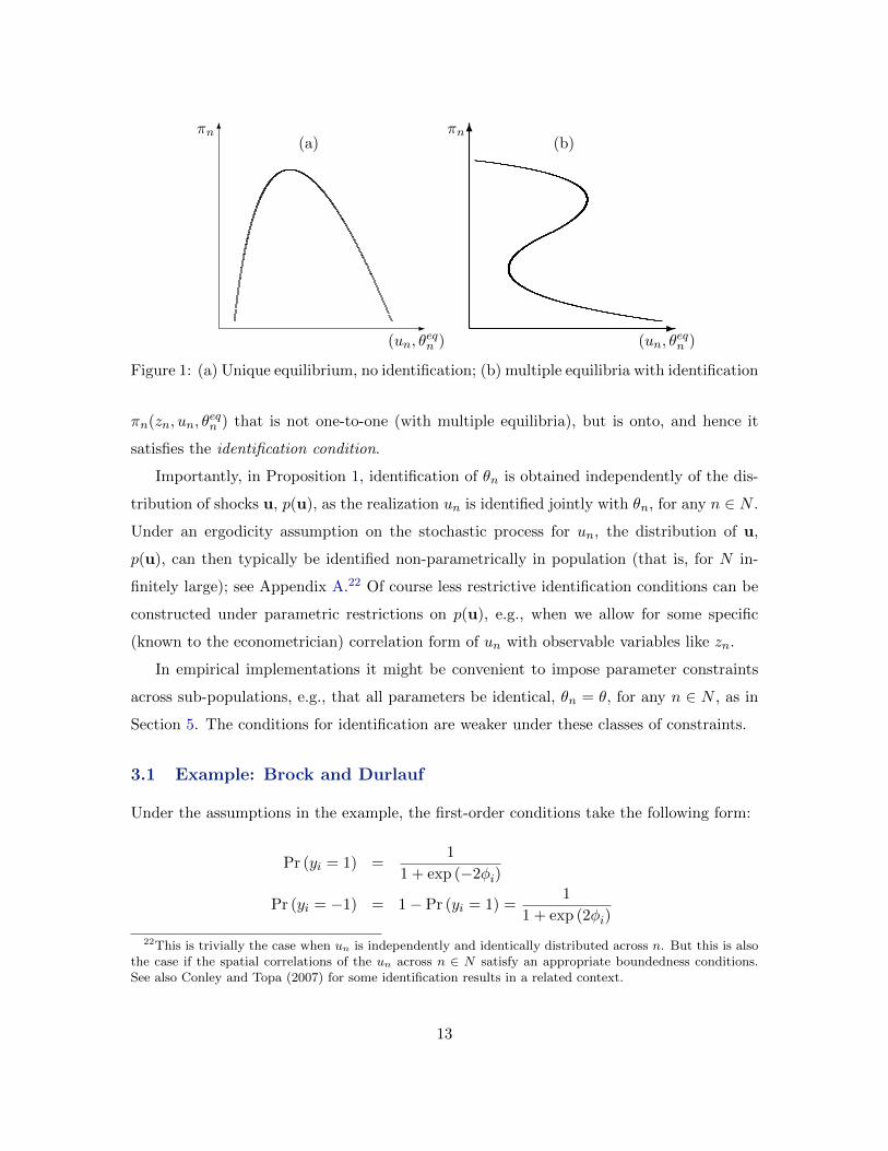
Note that the condition in Proposition 1 is not required for the uniqueness of equilibrium;

nor does uniqueness imply the condition.21 To illustrate this point, consider a society

characterized by a map P(πn, zn, un; θfocn ) which is one-to-one and onto. In this case,

identification rests on the properties of the map πn(zn, un, θeqn ), given zn. Panel (a) in

Figure 1 displays an equilibrium map that does not satisfy the condition for identification

in Proposition 1 even though the equilibrium is unique. Panel (b) displays a manifold

21A related result appears in Jovanovic (1989), who shows that a unique reduced form is neither a necessarynor sufficient condition for identification.

12

6

-(un, θ

eqn )

πn 6

-(un, θ

eqn )

πn(a) (b)

Figure 1: (a) Unique equilibrium, no identification; (b) multiple equilibria with identification

πn(zn, un, θeqn ) that is not one-to-one (with multiple equilibria), but is onto, and hence it

satisfies the identification condition.

Importantly, in Proposition 1, identification of θn is obtained independently of the dis-

tribution of shocks u, p(u), as the realization un is identified jointly with θn, for any n ∈ N .

Under an ergodicity assumption on the stochastic process for un, the distribution of u,

p(u), can then typically be identified non-parametrically in population (that is, for N in-

finitely large); see Appendix A.22 Of course less restrictive identification conditions can be

constructed under parametric restrictions on p(u), e.g., when we allow for some specific

(known to the econometrician) correlation form of un with observable variables like zn.

In empirical implementations it might be convenient to impose parameter constraints

across sub-populations, e.g., that all parameters be identical, θn = θ, for any n ∈ N , as in

Section 5. The conditions for identification are weaker under these classes of constraints.

3.1 Example: Brock and Durlauf

Under the assumptions in the example, the first-order conditions take the following form:

Pr (yi = 1) =1

1 + exp (−2φi)

Pr (yi = −1) = 1− Pr (yi = 1) =1

1 + exp (2φi)

22This is trivially the case when un is independently and identically distributed across n. But this is alsothe case if the spatial correlations of the un across n ∈ N satisfy an appropriate boundedness conditions.See also Conley and Topa (2007) for some identification results in a related context.

13

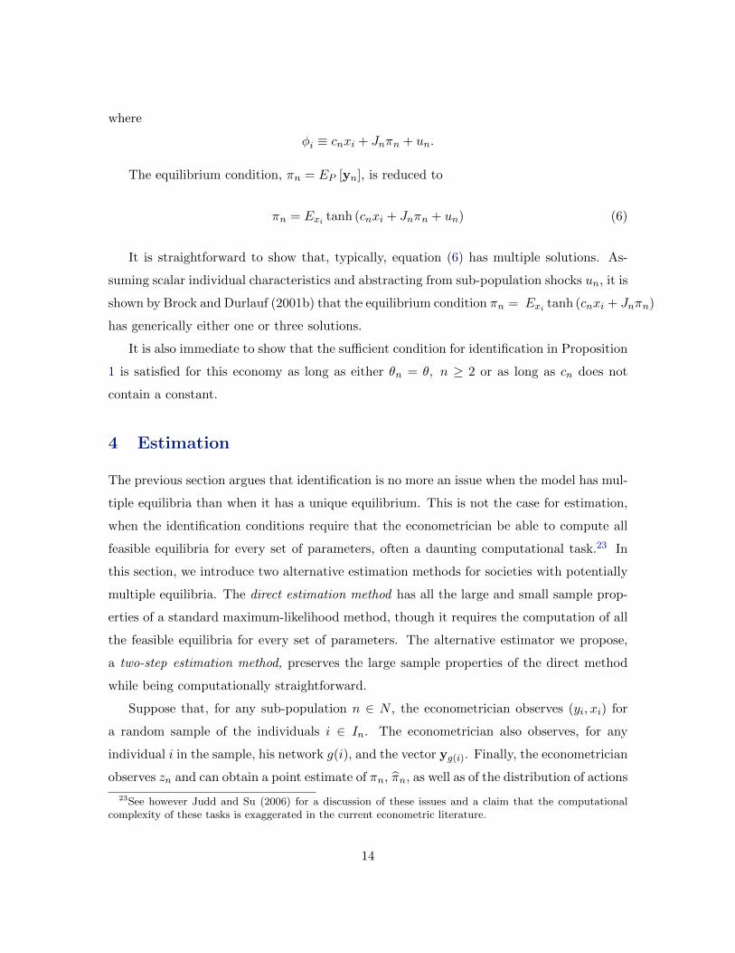
where

φi ≡ cnxi + Jnπn + un.

The equilibrium condition, πn = EP [yn], is reduced to

πn = Exi tanh (cnxi + Jnπn + un) (6)

It is straightforward to show that, typically, equation (6) has multiple solutions. As-

suming scalar individual characteristics and abstracting from sub-population shocks un, it is

shown by Brock and Durlauf (2001b) that the equilibrium condition πn = Exi tanh (cnxi + Jnπn)

has generically either one or three solutions.

It is also immediate to show that the sufficient condition for identification in Proposition

1 is satisfied for this economy as long as either θn = θ, n ≥ 2 or as long as cn does not

contain a constant.

4 Estimation

The previous section argues that identification is no more an issue when the model has mul-

tiple equilibria than when it has a unique equilibrium. This is not the case for estimation,

when the identification conditions require that the econometrician be able to compute all

feasible equilibria for every set of parameters, often a daunting computational task.23 In

this section, we introduce two alternative estimation methods for societies with potentially

multiple equilibria. The direct estimation method has all the large and small sample prop-

erties of a standard maximum-likelihood method, though it requires the computation of all

the feasible equilibria for every set of parameters. The alternative estimator we propose,

a two-step estimation method, preserves the large sample properties of the direct method

while being computationally straightforward.

Suppose that, for any sub-population n ∈ N , the econometrician observes (yi, xi) for

a random sample of the individuals i ∈ In. The econometrician also observes, for any

individual i in the sample, his network g(i), and the vector yg(i). Finally, the econometrician

observes zn and can obtain a point estimate of πn, πn, as well as of the distribution of actions

23See however Judd and Su (2006) for a discussion of these issues and a claim that the computationalcomplexity of these tasks is exaggerated in the current econometric literature.

14

and characteristics P (yn,xn | πn, zn, un), P (yn,xn | πn, zn, un). We assume that, for any

n ∈ N, the condition for identification in Proposition 1 is satisfied.

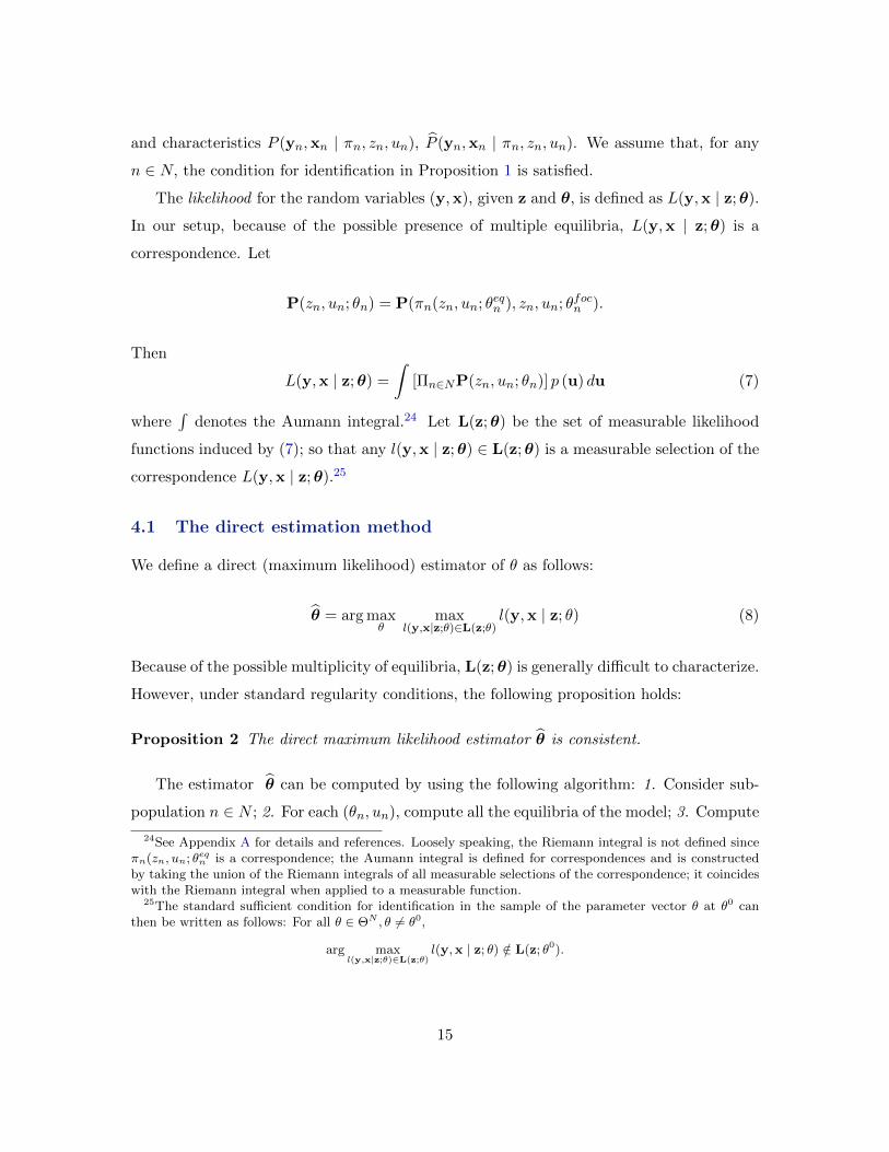
The likelihood for the random variables (y,x), given z and θ, is defined as L(y,x | z;θ).

In our setup, because of the possible presence of multiple equilibria, L(y,x | z;θ) is a

correspondence. Let

P(zn, un; θn) = P(πn(zn, un; θeqn ), zn, un; θfocn ).

Then

L(y,x | z;θ) =

∫[Πn∈NP(zn, un; θn)] p (u) du (7)

where∫

denotes the Aumann integral.24 Let L(z;θ) be the set of measurable likelihood

functions induced by (7); so that any l(y,x | z;θ) ∈ L(z;θ) is a measurable selection of the

correspondence L(y,x | z;θ).25

4.1 The direct estimation method

We define a direct (maximum likelihood) estimator of θ as follows:

θ = arg maxθ

maxl(y,x|z;θ)∈L(z;θ)

l(y,x | z; θ) (8)

Because of the possible multiplicity of equilibria, L(z;θ) is generally difficult to characterize.

However, under standard regularity conditions, the following proposition holds:

Proposition 2 The direct maximum likelihood estimator θ is consistent.

The estimator θ can be computed by using the following algorithm: 1. Consider sub-

population n ∈ N ; 2. For each (θn, un), compute all the equilibria of the model; 3. Compute

24See Appendix A for details and references. Loosely speaking, the Riemann integral is not defined sinceπn(zn, un; θeqn is a correspondence; the Aumann integral is defined for correspondences and is constructedby taking the union of the Riemann integrals of all measurable selections of the correspondence; it coincideswith the Riemann integral when applied to a measurable function.

25The standard sufficient condition for identification in the sample of the parameter vector θ at θ0 canthen be written as follows: For all θ ∈ ΘN , θ 6= θ0,

arg maxl(y,x|z;θ)∈L(z;θ)

l(y,x | z; θ) /∈ L(z; θ0).

15

the likelihood of each equilibrium and choose the maximum among them; 4. Repeat for all

n ∈ N ; 5. Integrate over u and maximize over θ. This procedure is computationally difficult,

especially when the society is sufficiently complex that a closed-form characterization of

equilibrium is impossible.

4.2 The two-step estimation method

We now introduce a simpler two-step estimation procedure.

First step. Compute the point estimates πn and P (yn,xn | πn, zn, un) for, respectively,

πn and P (yn,xn | πn, zn, un).

Second step. Estimate

(ˆun,ˆθeqn ) as a solution of

πn ∈ π(zn, ˆun,ˆθeqn );

and

ˆθfocn as a solution of

P (yn,xn | πn, zn, ˆun;ˆθfocn ) = P .

Note that this estimation procedure does not require the computation of all the equilibria

as a function of θn, because the inversion operations in the second step are guaranteed by

the identification condition. Note also that the inversion operations in the second step are

substituted e.g., by standard maximum likelihood procedures when parametric assumptions

are imposed on p(u) and/or when parameter constraints across sub-populations are imposed,

as in Section 5.

It is straightforward to conclude the following.

Proposition 3 If πn and P are consistent estimators of πn and P , the two-step estimatorˆθn is a consistent estimator of θn.

Furthermore, in specific empirical implementations, the small sample properties for the

two-step estimator can be improved by means of several expedients. First, the two-step

method can be iterated as, e.g., in Aguirregabiria and Mira (2007). Second, in constructing

16

the likelihood the econometrician could account for the distribution of the estimators πn

and P due, e.g., to sampling error.26

4.3 Monte Carlo analysis of estimators in Brock and Durlauf

We now study in detail the estimation methods in the previous section in the context of

the binary choice model of Brock and Durlauf (2001b), introduced in Section 2.2.

Because the model abstracts from local interactions, multiplicity in P (yn,xn | πn, zn, un),

for any πn, is not an issue. Assume without loss of generality that agents do not condition

on any zn. In this model, independence of εi across agents i ∈ I implies that, for the vector

of choices yn:

Pr (yn|xn, πn, un) =∏i

Pr (yi|xi, πn, un) ∼∏i

exp ((cnxi + un) · yi + Jnyiπn) (9)

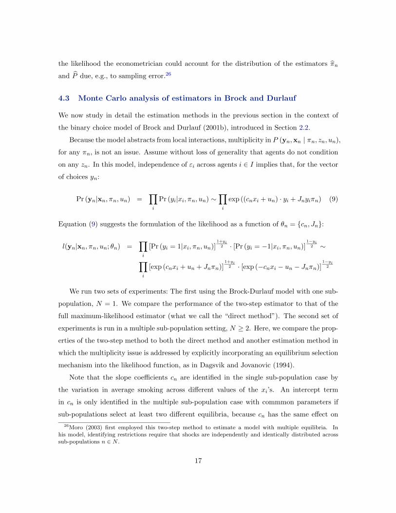
Equation (9) suggests the formulation of the likelihood as a function of θn = {cn, Jn}:

l(yn|xn, πn, un; θn) =∏i

[Pr (yi = 1|xi, πn, un)]1+yi

2 · [Pr (yi = −1|xi, πn, un)]1−yi

2 ∼

∏i

[exp (cnxi + un + Jnπn)]1+yi

2 · [exp (−cnxi − un − Jnπn)]1−yi

2

We run two sets of experiments: The first using the Brock-Durlauf model with one sub-

population, N = 1. We compare the performance of the two-step estimator to that of the

full maximum-likelihood estimator (what we call the “direct method”). The second set of

experiments is run in a multiple sub-population setting, N ≥ 2. Here, we compare the prop-

erties of the two-step method to both the direct method and another estimation method in

which the multiplicity issue is addressed by explicitly incorporating an equilibrium selection

mechanism into the likelihood function, as in Dagsvik and Jovanovic (1994).

Note that the slope coefficients cn are identified in the single sub-population case by

the variation in average smoking across different values of the xi’s. An intercept term

in cn is only identified in the multiple sub-population case with commmon parameters if

sub-populations select at least two different equilibria, because cn has the same effect on

26Moro (2003) first employed this two-step method to estimate a model with multiple equilibria. Inhis model, identifying restrictions require that shocks are independently and identically distributed acrosssub-populations n ∈ N .

17

Evaluation Criterion Direct Two-step Direct, two-step initial est

RMSE, parameter c 0.05056 0.05043 0.05043Bias, parameter c -0.00315 -0.00251 -0.00251

RMSE, parameter J 0.10768 0.10708 0.10706Bias, parameter J -0.00184 -0.00542 -0.00390

Min time 136.57404 0.23075 132.76532Max time 183.95280 0.36781 181.82902Mean time 157.22378 0.30190 158.34783

Median time 156.88555 0.29983 158.34823

Table 1: Monte Carlo single sub-population experiment - results (low-equilibrium)

behavior in all equilibria, but Jn’s effect is proportional to the equilibrium behavior. We

do not include an intercept term in any of our specifications.

4.3.1 Results for a single sub-population (N = 1)

We use a version of the Brock-Durlauf model with a single covariate xi ∼ N (µx, 1) and

global interactions (no local interactions). Thus the model parameters are a pair θ ≡ (c, J) ;

note that we drop the index n for simplicity as N = 1. We draw an artificial sample of

20,000 students (characterized by their attribute xi) and run a Monte-Carlo experiment,

drawing N =160 vectors of the true parameters of the model. Parameter c is drawn from

a uniform with support [−0.8, 0.8], and parameter J from a uniform with support [1, 3].

For each random draw θtruej of the model parameters, j = 1, ...,N , we use the model to

generate simulated data y(θtruej

), choosing one single equilibrium for a given experiment

(i.e., all students are acting according to the same equilibrium). For each simulated dataset

y(θtruej

)we estimate the model parameters using both the two-step and the direct methods,{

θ2s

j , θd

j

}, j = 1, ...,N . We then compare the properties of the two estimators, focusing

on several evaluation criteria: bias (the average difference between the estimator and the

true parameter), root mean squared error (RMSE) (the root of the average of the squared

differences between the estimator and the true parameter), and computational speed.

Table 1 reports the results of the experiments in which the low-level equilibrium was

always chosen; results for the intermediate and high-level equilibrium are very similar and

are available from the authors upon request. The second column reports properties of the

direct method where the starting value θ0 used in the likelihood maximization routine was

18

fixed at c = 0, J = 2. The third column reports statistics for the two-step method. The

fourth column reports results for the direct method when the two-step estimates θ2s

j were

used as initial values for the maximization algorithm.

The two-step method always exhibits lower RMSE than the direct method with fixed

starting values.27 This is surprising since the direct method represents the full maximum-

likelihood estimation and should therefore achieve a weakly lower RMSE. The reason for

this result is that, even though we use a maximization algorithm – simulated annealing –

that is very robust to discontinuities in the objective function, in a small but nontrivial

number of cases the algorithm gets “stuck” in a region of the parameters that correspond

to the wrong equilibrium, which yields estimates very far from θtrue. To address this issue,

we also use the direct method with θ2s

j as starting values (column four): in this case, the

RMSE is the same or slightly lower than in the two-step case.

The real advantage of the two-step method, however, is in computational speed. Even

with this very stripped-down model, an estimation run with the direct method took a

median time between 156 and 159 minutes (depending on the choice of equilibrium); instead,

the two-step method took roughly between twenty-seven and thirty seconds. This is a

vast computational advantage that enables researchers to estimate much richer models of

economic behavior than if they were to use brute force maximum-likelihood only.

4.3.2 Results for multiple sub-populations (N ≥ 2)

Our second set of experiments concerns a setting with multiple sub-populations n, where

all agents in a single sub-population n, i ∈ In, are assumed to be in the same equilibrium

but each sub-population may be in a different equilibrium.

A possible approach is to postulate a selection mechanism across equilibria, which in-

volves a specific correlation structure (in equilibria) across the different sub-populations of

the society (see, e.g., Dagsvik and Jovanovic (1994) and Bajari, Hong, and Ryan (2010)).

This enables the econometrician to write the likelihood as the product of two terms: loosely

speaking, the probability of the data in a given sub-population n, conditional on parameters

and on the equilibrium chosen in n; and the probability that sub-population n is in that

particular equilibrium given the selection mechanism. Therefore, the likelihood is a mixture

27The difference is slight in the case in which the low equilibrium is picked and larger in the other twocases, especially when the intermediate equilibrium is selected.

19

of likelihoods conditional on equilibria, where the weights are equal to the probabilities of

equilibria given data. Thus the likelihood becomes a well-behaved function rather than a

complicated correspondence. The downside of this approach is that the econometrician has

to take a stand on the specific equilibrium selection mechanism being used.

We perform two types of experimental comparisons. First, we again compare the two-

step estimator to the direct method. Second, we compare the two-step estimator with the

estimators obtained by postulating an equilibrium selection (we call this the D-J method, for

Dagsvik and Jovanovic). In the direct versus two-step method experiment, we use n = 20,

with 5,000 agents in each sub-population; in the D-J versus two-step method comparison,

we use n = 300, with 200 agents in each sub-population.28 To concentrate on equilibrium

selection, we assume the parameters are identical across sub-populations: (cn, Jn) = (c, J),

for all n, and are randomly drawn as in the single sub-population experiments. Suppose

the equilibrium set contains at most K equilibria, indexed by k = 1, ...,K. Let

φn (πk) = Pr (sub-population n is in eqm. πk |yn−1,yn−2, ...) .

To simulate the experimental data, we used a second-order spatially auto-regressive pro-

cess (SAR(2)) as our equilibrium selection mechanism. The sub-population is ordered on

a one-dimensional integer lattice, where “closeness” in the lattice represents “closeness” in

terms of social distance and hence it justifies the correlation structure imposed on equilib-

rium selection.29 Let K = 3, as in the Brock and Durlauf model we simulate. The first two

sub-populations are assigned one of the three possible equilibria at random (independently),

with probabilities (p1, p2, 1− p1 − p2). For n > 2, each sub-population n adopts the same

equilibrium as sub-population n−1 with probability a1, and it adopts the same equilibrium

as sub-population n − 2 with probability a2; with the residual probability (1− a1 − a2)

sub-population n is assigned an equilibrium independently of the preceding sub-population

(again with probabilities (p1, p2, 1− p1 − p2)). The conditional probabilities φn (πk) are

computed recursively based on this particular selection mechanism.

28We have a larger number of cities in the D-J experiment because we wanted to also study the method’sability to estimate the equilibrium selection mechanism; consequently, we were limited to having only 200artificial students in each sub-population n for computational reasons.

29In a time-series context, correlation across time-periods is perhaps more natural. In a cross-sectionalcontext, one can still determine “closeness” between sub-populations by using some notion of social distance:see Conley and Topa (2002).

20

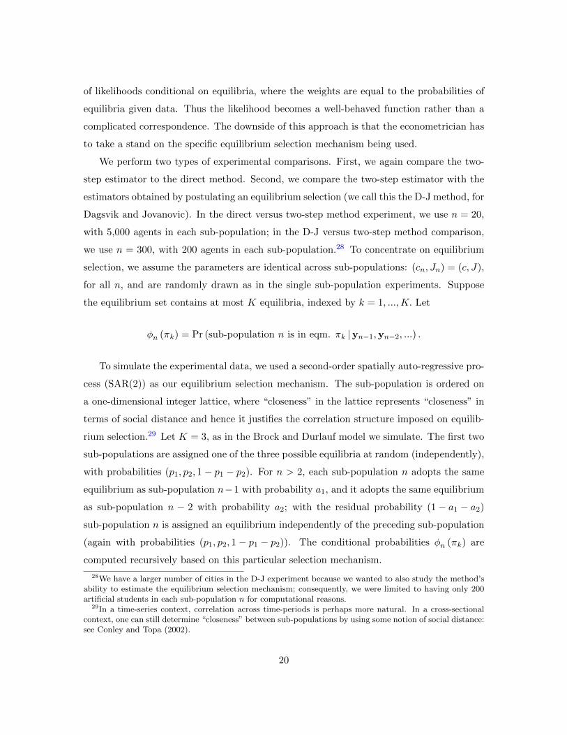
Correlation in eq. selection α1=α2=1/3 α1=0.1,α2=0.8Evaluation Criterion Direct Two-step Direct Two-step

(1) (2) (4) (5) (6)

RMSE, c 0.04849 0.00343 0.02468 0.02330Bias, c 0.00530 -0.00006 -0.00239 -0.00093RMSE, J 0.18000 0.02769 0.04941 0.04216Bias, J 0.03824 0.00705 0.00584 -0.00023Min time 133.07780 1.23348 130.13754 1.30992Max time 234.96883 6.49528 224.77100 7.60333Mean time 159.35291 1.57270 154.92274 1.65008Median time 157.15724 1.53797 152.82602 1.59336

Table 2: Monte Carlo multiple sub-populations experiments: comparison of direct andtwo-step methods

Table 2 collects results for the first set of experiments, comparing the two-step and direct

methods, where the evaluations are based on the results obtained from 160 runs where

the “true” parameters are randomly drawn using the same criteria used in the previous

subsection. The second and third columns concern an experiment in which the parameters

of the SAR(2) selection mechanism were set at a1 = 1/3, a2 = 1/3. In this particular case,

both RMSE and bias measures are much lower for the two-step than for the direct method.

We suspect that this is a consequence of the extreme computational difficulties involved

in maximizing the full likelihood in the multiple sub-populations case. As in the single

sub-population case, computational speed is again roughly two orders of magnitude higher

for the two-step method than for the direct method.

The RMSE and bias properties are quite sensitive to the specific parameterization of

the selection mechanism. Columns 4 and 5 display results for the case in which the SAR(2)

parameters are set at a1 = 1/10, a2 = 4/5. Here, the two methods under comparison

exhibit roughly similar properties in terms of RMSE and bias, although computational

speed is again much higher for the two-step method.

Finally, we turn to two experiments that perform a comparison between the two-step

and D-J methods. In each experiment, we wish to evaluate the performance of the D-J

method in the case in which the econometrician correctly specifies the equilibrium selection

process, as opposed to a situation in which the equilibrium selection is misspecified relative

to the truth. In the first experiment, the true selection mechanism is a SAR(2) process,

21

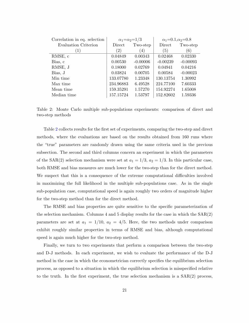
Econometrician Conjectures Correct: α1, α2 > 0 Misspecified: α2 = 0Evaluation Criterion D-J Two-step D-J Two-step

(1) (2) (3) (4) (5)

RMSE, C 0.00580 0.00736 0.00567 0.00721Bias, C -0.00015 -0.00027 -0.00032 -0.00036

RMSE, J 0.02455 0.04497 0.02390 0.04466Bias, J 0.00235 0.02343 0.00253 0.02302

Min time 330.61444 0.60659 277.07853 0.62736Median time 352.19753 0.74459 297.17443 0.73311

Max time 417.93318 2.32693 382.53198 5.82907

Table 3: Monte Carlo experiments: misspecification of the equilibrium transition probabil-ities

with a1 = 0.01, a2 = 0.95, whereas the econometrician assumes a SAR(1) specification in

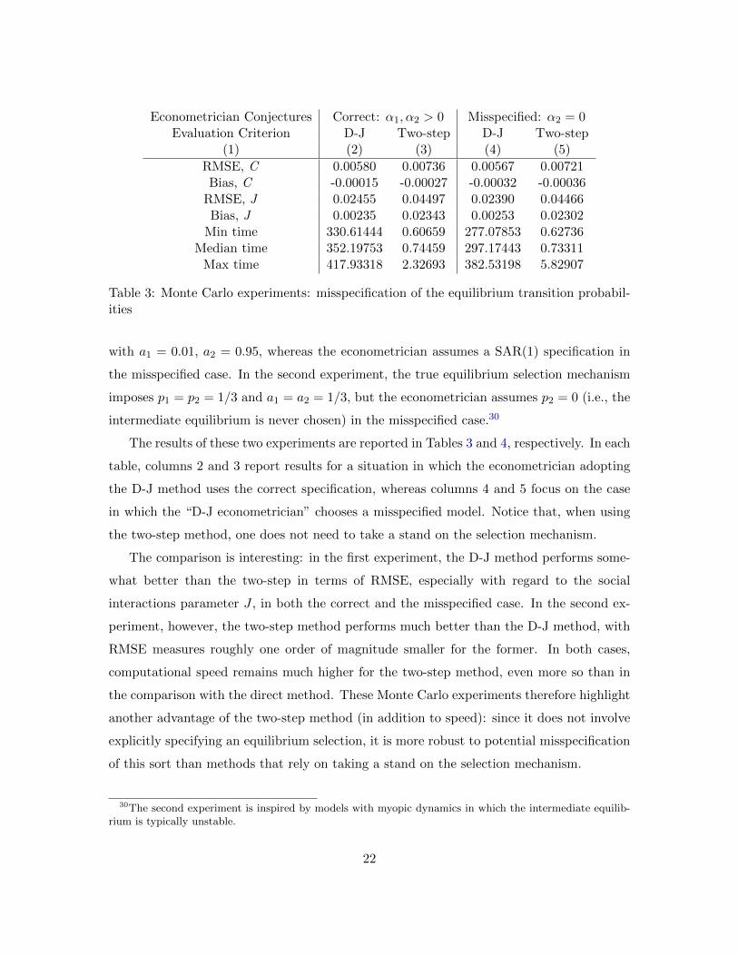
the misspecified case. In the second experiment, the true equilibrium selection mechanism

imposes p1 = p2 = 1/3 and a1 = a2 = 1/3, but the econometrician assumes p2 = 0 (i.e., the

intermediate equilibrium is never chosen) in the misspecified case.30

The results of these two experiments are reported in Tables 3 and 4, respectively. In each

table, columns 2 and 3 report results for a situation in which the econometrician adopting

the D-J method uses the correct specification, whereas columns 4 and 5 focus on the case

in which the “D-J econometrician” chooses a misspecified model. Notice that, when using

the two-step method, one does not need to take a stand on the selection mechanism.

The comparison is interesting: in the first experiment, the D-J method performs some-

what better than the two-step in terms of RMSE, especially with regard to the social

interactions parameter J , in both the correct and the misspecified case. In the second ex-

periment, however, the two-step method performs much better than the D-J method, with

RMSE measures roughly one order of magnitude smaller for the former. In both cases,

computational speed remains much higher for the two-step method, even more so than in

the comparison with the direct method. These Monte Carlo experiments therefore highlight

another advantage of the two-step method (in addition to speed): since it does not involve

explicitly specifying an equilibrium selection, it is more robust to potential misspecification

of this sort than methods that rely on taking a stand on the selection mechanism.

30The second experiment is inspired by models with myopic dynamics in which the intermediate equilib-rium is typically unstable.

22

Econometrician Conjectures Correct: P1, P2 > 0 Misspecified: P2 = 0Evaluation Criterion Jovanovic Two step Jovanovic Two step

(1) (2) (3) (4) (5)

RMSE, C 0.00517 0.00912 0.07751 0.00911Bias, C 0.00001 -0.00042 -0.01124 -0.00043

RMSE, J 0.02523 0.08002 0.74713 0.07953Bias, J 0.00437 0.05484 0.65119 0.05394

Min time 333.29544 0.59714 271.94123 0.62225Median time 356.65684 0.72343 287.05614 0.73007

Max time 453.14298 3.49153 398.08752 0.84737

Table 4: Monte Carlo experiments: misspecification of the equilibrium selection probabili-ties

5 Social interactions and smoking

In this section, we estimate several different specifications of the social interactions model

in Brock and Durlauf (2001b), presented in Section 2.2. To this end, we use data on smok-

ing obtained from the National Longitudinal Study of Adolescent Health (Add Health), a

longitudinal study of a nationally representative sample of adolescents in grades seven to

twelve in the United States during the 1994-95 school year. Add Health combines longitu-

dinal survey data on respondents’ social, economic, psychological, and physical well-being

with contextual data on the family, neighborhood, community, school, friendships, peer

groups, and romantic relationships. A sample of eighty U.S. high schools and fifty-two U.S.

middle schools was selected with unequal probability of selection. Incorporating systematic

sampling methods and implicit stratification into the Add Health study design ensured this

sample is representative of U.S. schools with respect to region of the country, urban or rural

setting, school size, school type, and ethnic composition.

In the empirical application, therefore, we encode yi = 1 if agent i smokes and yi = −1 if

he or she does not. Each sub-population n is a school. We consider only high schools, which

we define as schools having students enrolled in all grades between nine and twelve. Among

these, we include only the forty-five schools that have at least 400 students, in order to have

a sufficient number of smokers and minorities in each school. Even with these restrictions,

there are cases in which the parameter estimates associated with specific racial or ethnic

groups are not estimated with any precision.

23

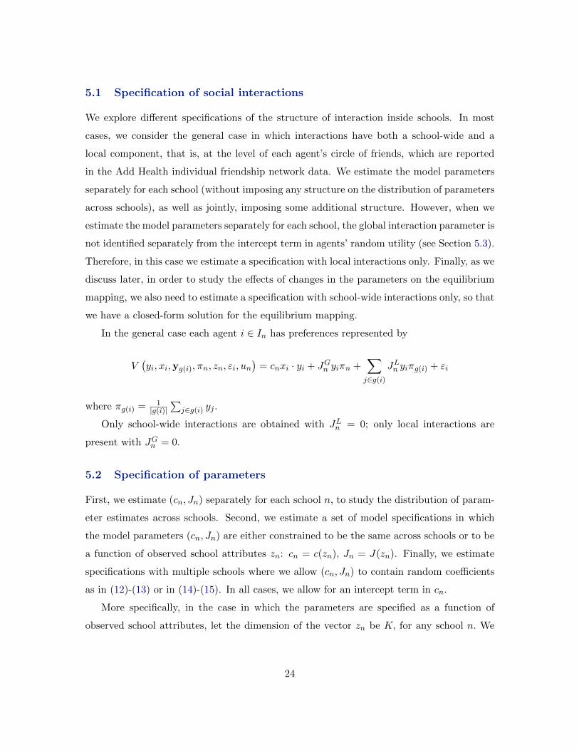
5.1 Specification of social interactions

We explore different specifications of the structure of interaction inside schools. In most

cases, we consider the general case in which interactions have both a school-wide and a

local component, that is, at the level of each agent’s circle of friends, which are reported

in the Add Health individual friendship network data. We estimate the model parameters

separately for each school (without imposing any structure on the distribution of parameters

across schools), as well as jointly, imposing some additional structure. However, when we

estimate the model parameters separately for each school, the global interaction parameter is

not identified separately from the intercept term in agents’ random utility (see Section 5.3).

Therefore, in this case we estimate a specification with local interactions only. Finally, as we

discuss later, in order to study the effects of changes in the parameters on the equilibrium

mapping, we also need to estimate a specification with school-wide interactions only, so that

we have a closed-form solution for the equilibrium mapping.

In the general case each agent i ∈ In has preferences represented by

V(yi, xi,yg(i), πn, zn, εi, un

)= cnxi · yi + JGn yiπn +

∑j∈g(i)

JLn yiπg(i) + εi

where πg(i) = 1|g(i)|

∑j∈g(i) yj .

Only school-wide interactions are obtained with JLn = 0; only local interactions are

present with JGn = 0.

5.2 Specification of parameters

First, we estimate (cn, Jn) separately for each school n, to study the distribution of param-

eter estimates across schools. Second, we estimate a set of model specifications in which

the model parameters (cn, Jn) are either constrained to be the same across schools or to be

a function of observed school attributes zn: cn = c(zn), Jn = J(zn). Finally, we estimate

specifications with multiple schools where we allow (cn, Jn) to contain random coefficients

as in (12)-(13) or in (14)-(15). In all cases, we allow for an intercept term in cn.

More specifically, in the case in which the parameters are specified as a function of

observed school attributes, let the dimension of the vector zn be K, for any school n. We

24

adopt the following linear specification:

cn = c(zn) = α0 +K∑k=1

αkzkn; (10)

Jn = J(zn) = γ0 +

K∑k=1

γkzkn. (11)

In the case in which we let the parameters contain random coefficients, the specification

we adopt is:

cn = α0 + αn, with αn ∼ N(0, σα) (12)

Jn = γ0 + γn, with γn ∼ N(0, σγ) (13)

More generally, we also include school attributes zn:

cn = α0 +K∑k=1

αkzkn + αn, with αn ∼ N(0, σα) (14)

Jn = γ0 +

K∑k=1

γkzkn + γn, with γn ∼ N(0, σγ) (15)

We assume that the random coefficients {αn, γn} are independent of each other and of

the individual random terms εi(yi) that enter the individuals’ random utilities. We specify

a functional form for the probability distribution of {αn, γn} in order to put some structure

on the distribution of the realized {cn, Jn}.

5.3 Identification of parameters

In the general case presented above, where the estimation is run on data from all schools

jointly, the parameters(cn, J

Ln , J

Gn

)are identified separately by the variation in demographic

attributes within schools, in smoking prevalence across personal networks, and in school-

wide smoking prevalence across schools. The parameter ruling school-wide interactions,

JGn , is identified separately from the intercept in cn – which is assumed constant across

schools – by the variation in the fraction of smokers across schools. The parameter for

local interactions, JLn , is identified by the variation in smoking behavior across personal

25

friendship networks, both within and across schools.

In a single-school setting, the school-wide interaction parameter is identified separately

from the slope coefficients in cn as long as there is some variation in demographic attributes

within the school. Similarly, the local interaction parameter is identified as long as there

is some variation in smoking prevalence across individual networks. However, JGn is not

identified separately from the intercept term in cn. Therefore, in the school-by-school

estimation we present below, we focus on the specification with local interactions only,

arbitrarily setting JGn = 0.

5.4 Empirical results

In what follows, we present summaries of the parameter estimates for a selection of spec-

ifications. Standard errors of the parameter estimates were computed using the bootstrap

method. We then perform some simulation exercises to compute the estimated effect on

the incidence on smoking of changes in the level of social interactions.

In the general case in which interactions have both a school-wide (“global”) and a

local (personal network) component, and random fixed effects {αn, γn} are added to the

parameters, the likelihood of the data yn given πn,[πg(i)

]i∈In

, θn in school n is:

log L(yn|πn,[πg(i)

]i∈In

; θn) =

−∑i∈In

(1+yi2

)· log

(1 + exp

[−2(cnxi + JGn πn + JLn πg(i)

)])+(1−yi2

)· log

(1 + exp

[2(cnxi + JGn πn + JLn πg(i)

)])

+ Pr(αn) + Pr(γn).

5.4.1 School-by-school estimation

In this section, the model parameters are estimated separately for each school, that is we

maximize a separate likelihood for each school. (See Section 5.3 for a discussion of identi-

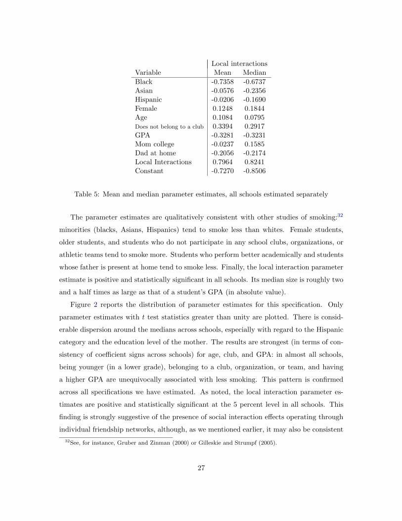
fication in this case.) Table 5 reports the means and medians of the parameter estimates

across schools for the specification with local interactions only because, as discussed earlier,

the global interaction parameter is not identified separately from the constant in this case31.

31The parameter estimates for each school are available from the authors upon request.

26

Local interactionsVariable Mean Median

Black -0.7358 -0.6737Asian -0.0576 -0.2356Hispanic -0.0206 -0.1690Female 0.1248 0.1844Age 0.1084 0.0795Does not belong to a club 0.3394 0.2917GPA -0.3281 -0.3231Mom college -0.0237 0.1585Dad at home -0.2056 -0.2174Local Interactions 0.7964 0.8241Constant -0.7270 -0.8506

Table 5: Mean and median parameter estimates, all schools estimated separately

The parameter estimates are qualitatively consistent with other studies of smoking:32

minorities (blacks, Asians, Hispanics) tend to smoke less than whites. Female students,

older students, and students who do not participate in any school clubs, organizations, or

athletic teams tend to smoke more. Students who perform better academically and students

whose father is present at home tend to smoke less. Finally, the local interaction parameter

estimate is positive and statistically significant in all schools. Its median size is roughly two

and a half times as large as that of a student’s GPA (in absolute value).

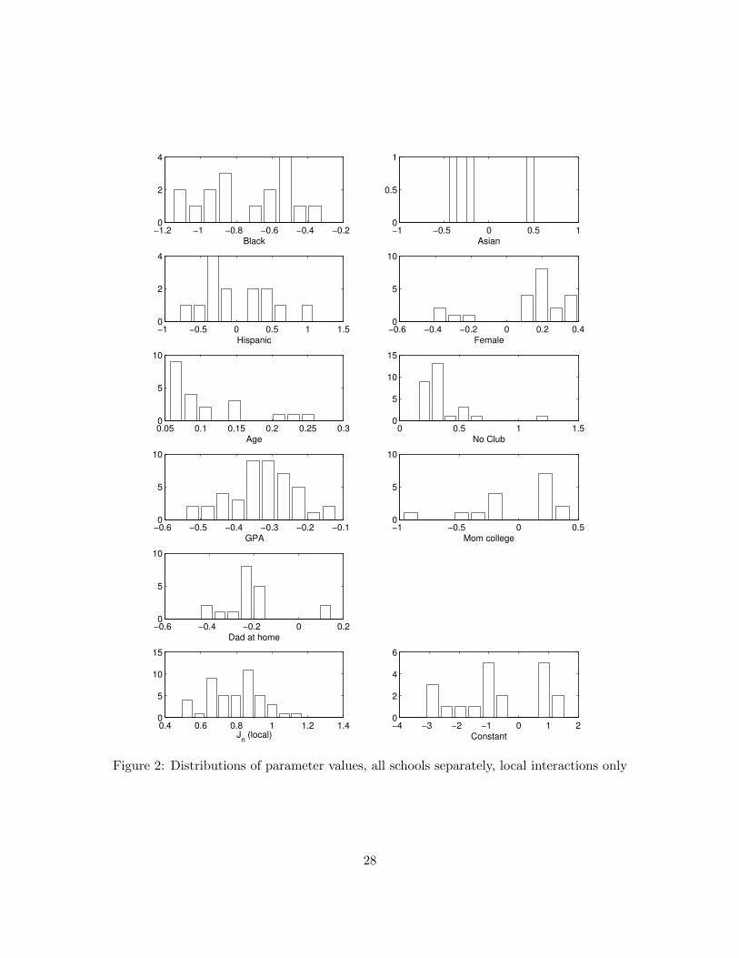
Figure 2 reports the distribution of parameter estimates for this specification. Only

parameter estimates with t test statistics greater than unity are plotted. There is consid-

erable dispersion around the medians across schools, especially with regard to the Hispanic

category and the education level of the mother. The results are strongest (in terms of con-

sistency of coefficient signs across schools) for age, club, and GPA: in almost all schools,

being younger (in a lower grade), belonging to a club, organization, or team, and having

a higher GPA are unequivocally associated with less smoking. This pattern is confirmed

across all specifications we have estimated. As noted, the local interaction parameter es-

timates are positive and statistically significant at the 5 percent level in all schools. This

finding is strongly suggestive of the presence of social interaction effects operating through

individual friendship networks, although, as we mentioned earlier, it may also be consistent

32See, for instance, Gruber and Zinman (2000) or Gilleskie and Strumpf (2005).

27

−1.2 −1 −0.8 −0.6 −0.4 −0.20

2

4

Black−1 −0.5 0 0.5 10

0.5

1

Asian

−1 −0.5 0 0.5 1 1.50

2

4

Hispanic−0.6 −0.4 −0.2 0 0.2 0.40

5

10

Female

0.05 0.1 0.15 0.2 0.25 0.30

5

10

Age0 0.5 1 1.5

0

5

10

15

No Club

−0.6 −0.5 −0.4 −0.3 −0.2 −0.10

5

10

GPA−1 −0.5 0 0.50

5

10

Mom college

−0.6 −0.4 −0.2 0 0.20

5

10

Dad at home

0.4 0.6 0.8 1 1.2 1.40

5

10

15

Jn (local)−4 −3 −2 −1 0 1 20

2

4

6

Constant

Figure 2: Distributions of parameter values, all schools separately, local interactions only

28

Variable Coefficient Std. err.

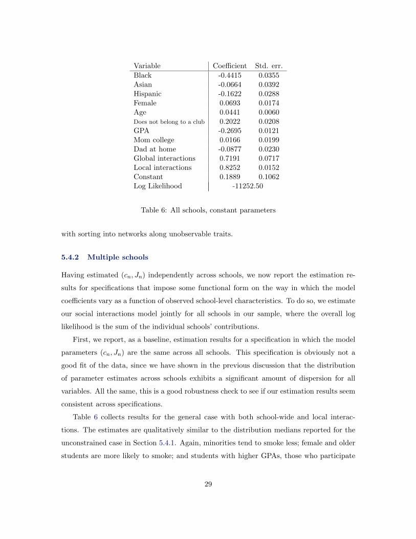
Black -0.4415 0.0355Asian -0.0664 0.0392Hispanic -0.1622 0.0288Female 0.0693 0.0174Age 0.0441 0.0060Does not belong to a club 0.2022 0.0208GPA -0.2695 0.0121Mom college 0.0166 0.0199Dad at home -0.0877 0.0230Global interactions 0.7191 0.0717Local interactions 0.8252 0.0152Constant 0.1889 0.1062Log Likelihood -11252.50

Table 6: All schools, constant parameters

with sorting into networks along unobservable traits.

5.4.2 Multiple schools

Having estimated (cn, Jn) independently across schools, we now report the estimation re-

sults for specifications that impose some functional form on the way in which the model

coefficients vary as a function of observed school-level characteristics. To do so, we estimate

our social interactions model jointly for all schools in our sample, where the overall log

likelihood is the sum of the individual schools’ contributions.

First, we report, as a baseline, estimation results for a specification in which the model

parameters (cn, Jn) are the same across all schools. This specification is obviously not a

good fit of the data, since we have shown in the previous discussion that the distribution

of parameter estimates across schools exhibits a significant amount of dispersion for all

variables. All the same, this is a good robustness check to see if our estimation results seem

consistent across specifications.

Table 6 collects results for the general case with both school-wide and local interac-

tions. The estimates are qualitatively similar to the distribution medians reported for the

unconstrained case in Section 5.4.1. Again, minorities tend to smoke less; female and older

students are more likely to smoke; and students with higher GPAs, those who participate

29

in school organizations or teams, and those whose fathers are present at home smoke less.

The parameter estimate for local interactions is very similar in magnitude to the median

estimate for the case in which each school is treated separately. The school-wide interaction

parameter, which is identified in this specification because of the variation in smoking preva-

lence across schools, is slightly smaller than that for local interactions, but still positive and

statistically significant at the 1 percent level.

Next, we turn to a specification in which parameters – while still deterministic – are a

function of observed school attributes zn, as in equations (10) and (11). We have chosen

the following list of attributes describing the presence of tobacco-related policies at a given

school: whether the school enacts state-mandated training on the use of tobacco products,

whether the school has implemented rules regarding the use of tobacco products by students,

and whether the school has implemented rules regarding the use of tobacco products by its

staff. We have also added the following list of attributes pertaining to the county in which

the school is located: whether the county is urban or rural, the percentage of families under

the poverty line, the fraction of college-educated individuals in the population twenty-five

years and older; and the fraction of female (male) adults in the labor force.

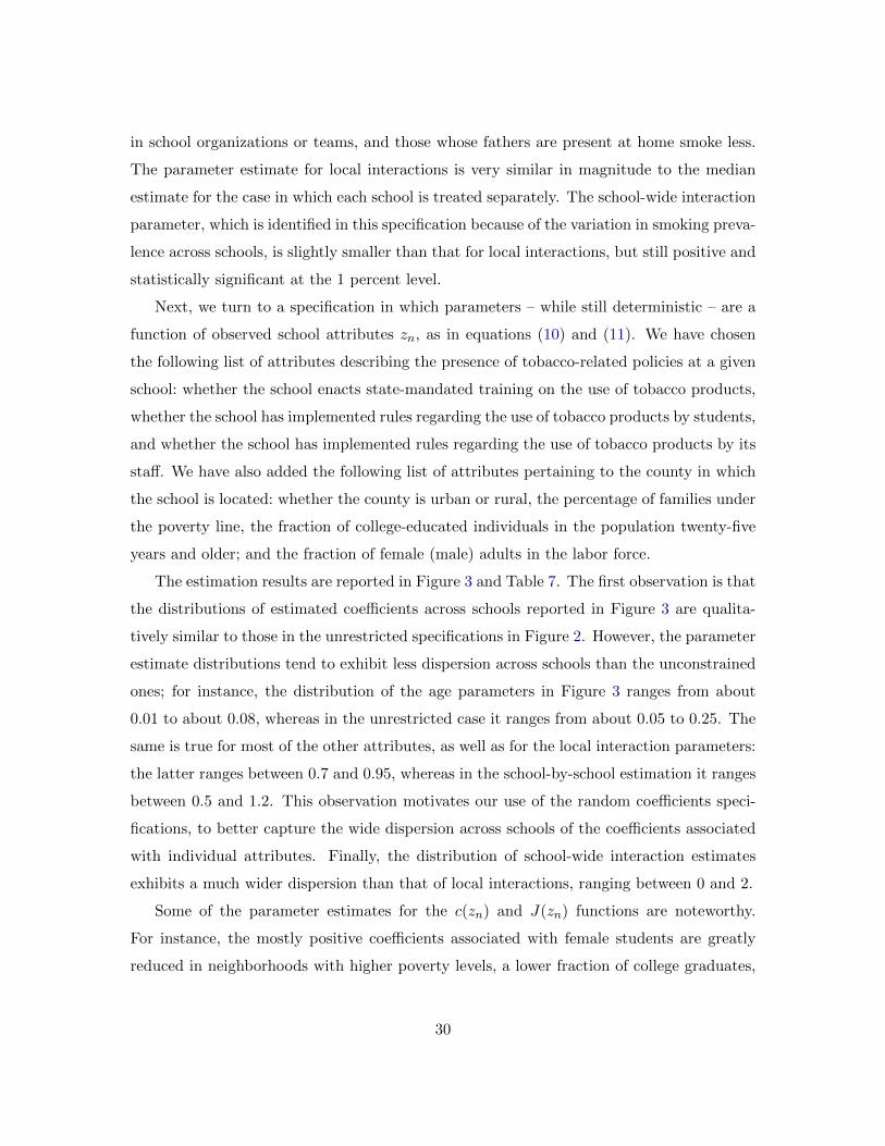
The estimation results are reported in Figure 3 and Table 7. The first observation is that

the distributions of estimated coefficients across schools reported in Figure 3 are qualita-

tively similar to those in the unrestricted specifications in Figure 2. However, the parameter

estimate distributions tend to exhibit less dispersion across schools than the unconstrained

ones; for instance, the distribution of the age parameters in Figure 3 ranges from about

0.01 to about 0.08, whereas in the unrestricted case it ranges from about 0.05 to 0.25. The

same is true for most of the other attributes, as well as for the local interaction parameters:

the latter ranges between 0.7 and 0.95, whereas in the school-by-school estimation it ranges

between 0.5 and 1.2. This observation motivates our use of the random coefficients speci-

fications, to better capture the wide dispersion across schools of the coefficients associated

with individual attributes. Finally, the distribution of school-wide interaction estimates

exhibits a much wider dispersion than that of local interactions, ranging between 0 and 2.

Some of the parameter estimates for the c(zn) and J(zn) functions are noteworthy.

For instance, the mostly positive coefficients associated with female students are greatly

reduced in neighborhoods with higher poverty levels, a lower fraction of college graduates,

30

−0.4 −0.2 0 0.2 0.40

5

10

15Distribution of C−female (C = C(Z)); all

0 0.02 0.04 0.06 0.08 0.10

5

10

15Distribution of C−age (C = C(Z)); all

0 0.1 0.2 0.3 0.40

5

10

15

20Distribution of C−noclub (C = C(Z)); all

−0.3 −0.25 −0.2 −0.15 −0.10

5

10

15Distribution of C−gradeavg (C = C(Z)); all

−0.2 −0.1 0 0.1 0.20

5

10

15Distribution of C−momcollege (C = C(Z)); all

−0.2 −0.15 −0.1 −0.05 0 0.050

2

4

6

8

10Distribution of C−dadhome (C = C(Z)); all

0.7 0.75 0.8 0.85 0.9 0.95 10

5

10

15Distribution of J−local (J = J(Z)); all

−0.5 0 0.5 1 1.5 2 2.50

2

4

6

8Distribution of J−global (G = G(Z)); all

Figure 3: Distributions of parameter values, all schools, deterministic coefficients functionof school characteristics

31

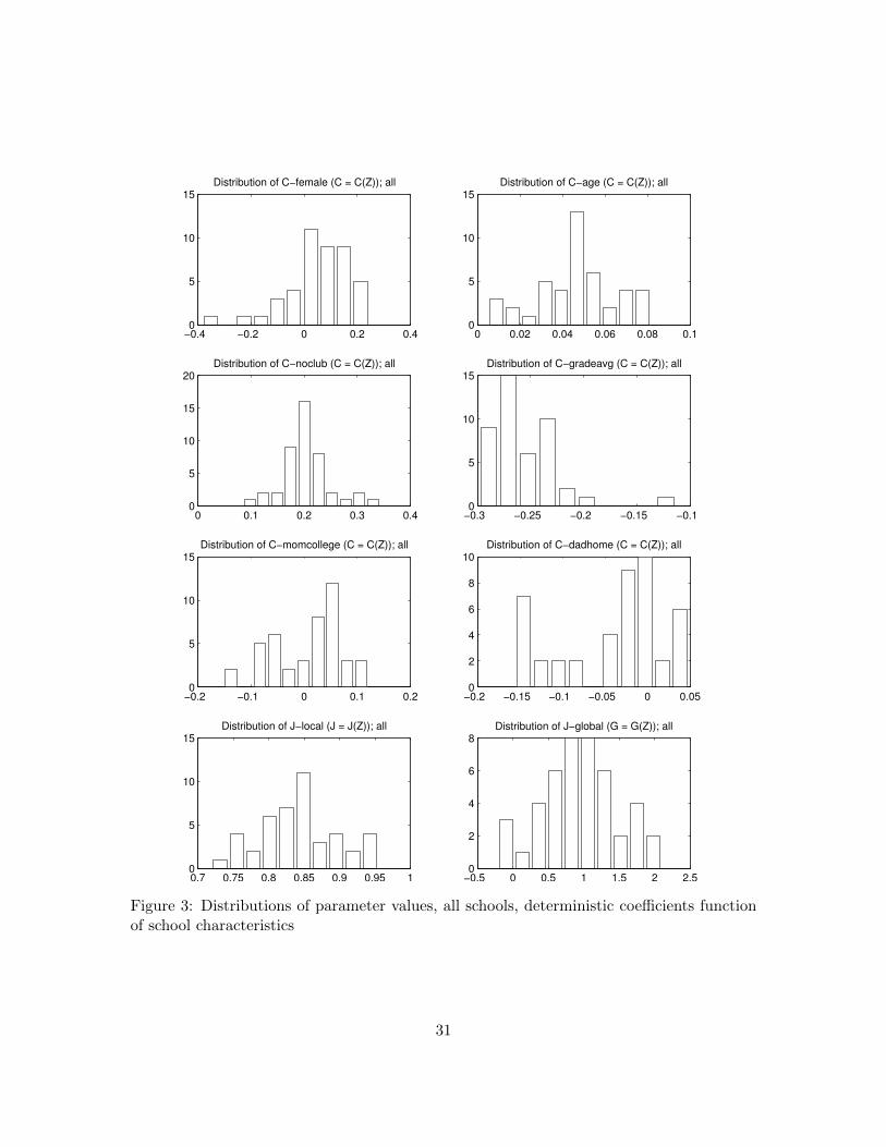
Female Age No clubIntercept 1.4904 (0.1300) -0.0037 (0.0067) -0.5867 (0.2113)% Urban 0.0034 (0.0601) 0.0333 (0.0080) -0.0122 (0.0726)% Poverty -1.6764 (0.3644) 0.1857 (0.0400) 0.4575 (0.4327)% College over 25 0.6127 (0.3485) 0.0370 (0.0238) 0.2228 (0.4275)Female Labor Force P.R. -1.4867 (0.2978) -0.0900 (0.0133) 0.9968 (0.5351)Male Labor Force P.R. -0.8336 (0.1841) 0.0106 (0.0076) 0.2586 (0.3100)Tobacco training -0.0888 (0.0379) 0.0223 (0.0058) 0.0122 (0.0482)Tobacco student policy 0.0922 (0.0880) -0.0179 (0.0068) 0.2056 (0.1004)Tobacco staff policy -0.1237 (0.0882) 0.0388 (0.0061) -0.1809 (0.0956)

GPA Mom college Dad HomeIntercept 0.1427 (0.0325) -0.3879 (0.1720) -0.2364 (0.0966)% Urban 0.0001 (0.0370) 0.1338 (0.0730) -0.0185 (0.0707)% Poverty 0.0711 (0.1740) -0.0321 (0.3909) 0.3613 (0.3915)% College over 25 -0.0967 (0.1322) -0.4370 (0.3739) 0.2692 (0.3856)Female Labor Force P.R. -0.4700 (0.0734) -0.4900 (0.4452) -0.6471 (0.2632)Male Labor Force P.R. -0.1830 (0.0449) 0.9316 (0.2464) 0.4012 (0.1495)Tobacco training -0.0128 (0.0245) -0.0264 (0.0457) 0.1201 (0.0485)Tobacco student policy -0.0375 (0.0386) -0.0075 (0.1104) -0.1367 (0.0996)Tobacco staff policy 0.0106 (0.0402) -0.0205 (0.1065) 0.1388 (0.0923)

Local Inter. Global Inter. ConstantIntercept 0.3394 (0.1373) 2.5743 (0.1562) 0.1882 (0.1099)% Urban -0.1048 (0.0517) 0.9509 (0.1878)% Poverty -0.2967 (0.3193) 4.4323 (0.7985)% College over 25 -0.0294 (0.2953) 1.2494 (0.6009)Female Labor Force P.R. 0.5911 (0.3383) -6.8403 (0.3243)Male Labor Force P.R. 0.5800 (0.2016) -0.8632 (0.1961)Tobacco training -0.0403 (0.0397) 0.6166 (0.1487)Tobacco student policy 0.0038 (0.0821) -0.6505 (0.1554)Tobacco staff policy -0.0951 (0.0816) 1.0344 (0.1506)

Table 7: All schools, deterministic coefficients function of school characteristics (standarderrors in parenthesis, log likelihood -11130.5654)

and higher female labor force participation, suggesting that female smoking may be related

to higher socioeconomic status. The positive relationship between student age and smoking

is stronger in higher poverty areas. The finding that Dad’s presence at home is associated

with less smoking is reinforced in neighborhoods with higher female labor force participation,

perhaps indicating that one parent’s presence and control is even more crucial when the

other parent works outside the home.

Interestingly, a school’s tobacco-related policies can have a large impact on the strength

of the social interaction terms. The presence of tobacco rules for students is associated with

lower school-wide interactions parameters, whereas tobacco training programs and tobacco

rules for the staff seem to increase the strength of school-wide interactions but slightly

reduce the strength of local interactions (however, the latter estimates are not statistically

significant). Of course, these school policy variables are likely endogenous, but the finding

32

that various tobacco policies may be related to stronger or weaker social interaction terms

is important, and we will return to it in our discussion of counterfactual experiments.

Finally, it is worth noting that neighborhood poverty levels and female labor force

participation have a very large impact on school-wide interactions estimates. This suggests

that some of the variation in smoking across schools that is unexplained by observed student

attributes and is attributed in the estimation to school-wide interaction effects may in fact

be a school-wide fixed effect related to the area’s socioeconomic status and other attributes.

This possibility stresses the value of having individual friendship network data to estimate

local social interaction effects.

5.4.3 Multiple schools, random coefficients

As mentioned in the previous section, letting (cn, Jn) depend on observed school charac-

teristics in a deterministic fashion may not be sufficient to capture the wide variation of

parameter estimates across schools found in the unrestricted case. Therefore, we also use

the random coefficient specification described in Section 5.2, to better capture the dispersion

in coefficient values across schools. We first estimate a version with only an intercept and a

random term, as in (12)-(13), and then augment it with school-level characteristics zn as in

(14)-(15). For computational feasibility, we use only two individual student attributes – age

and grade point average – since the introduction of random coefficients raises considerably

the number of parameters to be estimated.

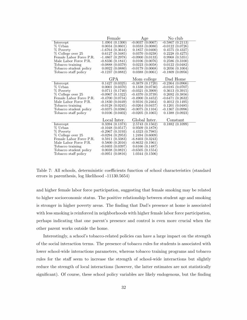
Figure 4 reports the distributions of the estimated parameters for two specifications

without zn: with only school-wide interactions (left three panes) and with both school-

wide and local interactions (right four panes). Results are qualitatively consistent with the

specifications presented so far. As expected, the range of values for the age, GPA, and

local interaction coefficients is wider than in the deterministic case (Figure 3) and very

similar to that of the unrestricted school-by-school specification (Figure 2). Introducing

local interaction effects generally lowers the school-wide interactions estimates relative to

the case with school-wide interactions only.

Interestingly, we find a very large dispersion in the strength of school-wide social inter-

action effects, ranging roughly between zero and eight. We conjecture that this dispersion

may reflect differences across schools in terms of neighborhood attributes, or in the extent

33

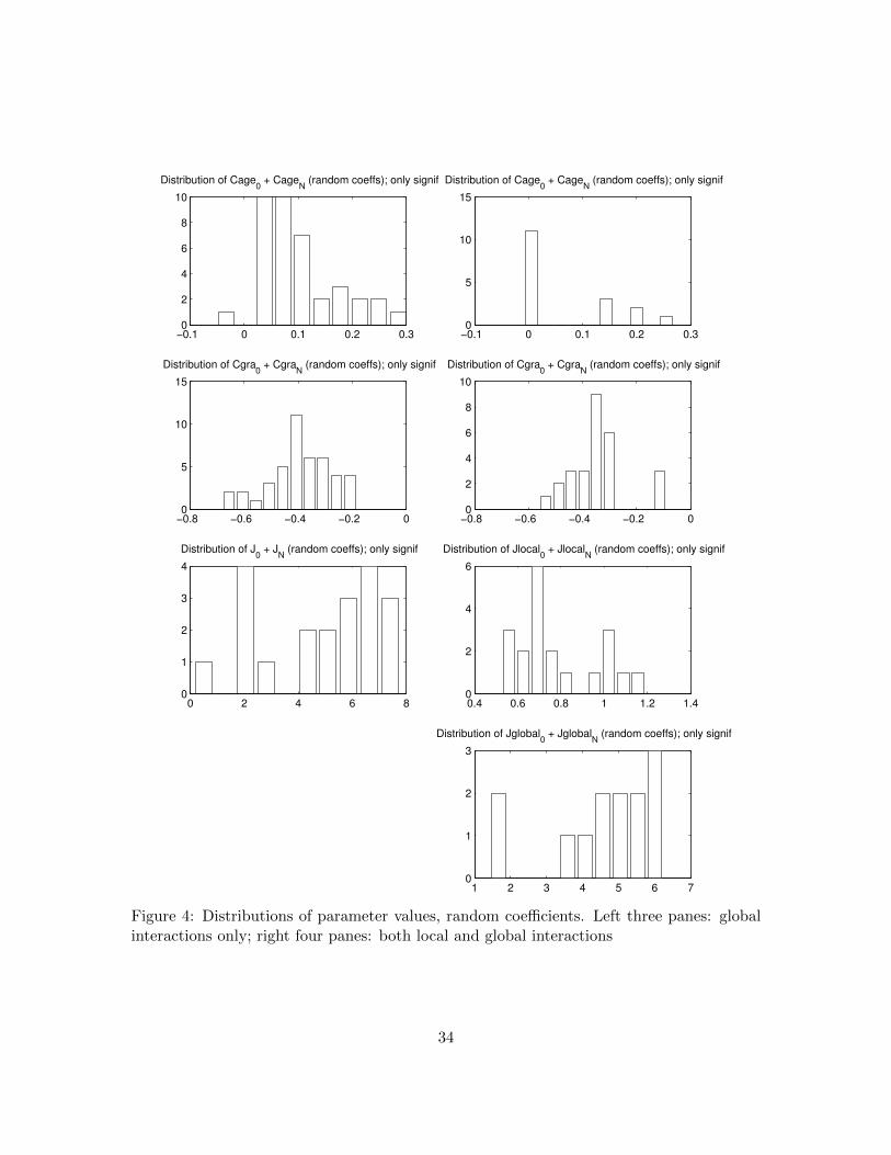
−0.1 0 0.1 0.2 0.30

2

4

6

8

10Distribution of Cage0 + CageN (random coeffs); only signif

−0.8 −0.6 −0.4 −0.2 00

5

10

15Distribution of Cgra0 + CgraN (random coeffs); only signif

0 2 4 6 80

1

2

3

4Distribution of J0 + JN (random coeffs); only signif

−0.1 0 0.1 0.2 0.30

5

10

15Distribution of Cage0 + CageN (random coeffs); only signif

−0.8 −0.6 −0.4 −0.2 00

2

4

6

8

10Distribution of Cgra0 + CgraN (random coeffs); only signif

0.4 0.6 0.8 1 1.2 1.40

2

4

6Distribution of Jlocal0 + JlocalN (random coeffs); only signif

1 2 3 4 5 6 70

1

2

3Distribution of Jglobal0 + JglobalN (random coeffs); only signif

Figure 4: Distributions of parameter values, random coefficients. Left three panes: globalinteractions only; right four panes: both local and global interactions

34

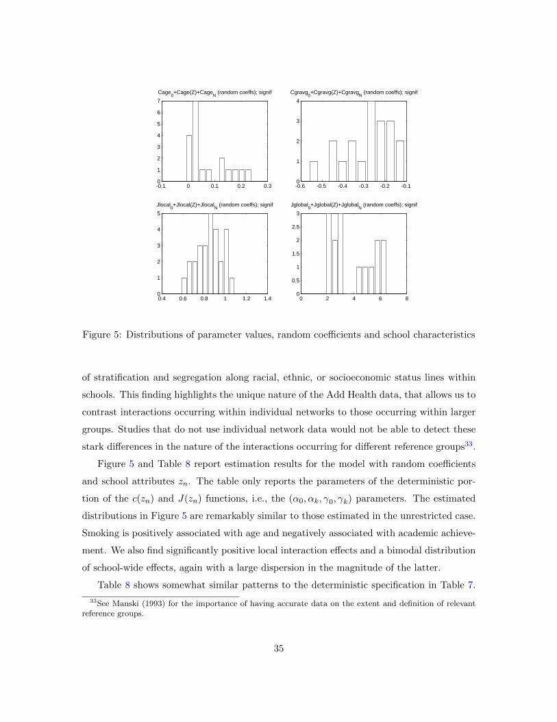
-0.1 0 0.1 0.2 0.30

1

2

3

4

5

6

7Cage0+Cage(Z)+CageN (random coeffs); signif

-0.6 -0.5 -0.4 -0.3 -0.2 -0.10

1

2

3

4Cgravg0+Cgravg(Z)+CgravgN (random coeffs); signif

0.4 0.6 0.8 1 1.2 1.40

1

2

3

4

5Jlocal0+Jlocal(Z)+JlocalN (random coeffs); signif

0 2 4 6 80

0.5

1

1.5

2

2.5

3Jglobal0+Jglobal(Z)+JglobalN (random coeffs); signif

Figure 5: Distributions of parameter values, random coefficients and school characteristics

of stratification and segregation along racial, ethnic, or socioeconomic status lines within

schools. This finding highlights the unique nature of the Add Health data, that allows us to

contrast interactions occurring within individual networks to those occurring within larger

groups. Studies that do not use individual network data would not be able to detect these

stark differences in the nature of the interactions occurring for different reference groups33.

Figure 5 and Table 8 report estimation results for the model with random coefficients

and school attributes zn. The table only reports the parameters of the deterministic por-

tion of the c(zn) and J(zn) functions, i.e., the (α0, αk, γ0, γk) parameters. The estimated

distributions in Figure 5 are remarkably similar to those estimated in the unrestricted case.

Smoking is positively associated with age and negatively associated with academic achieve-

ment. We also find significantly positive local interaction effects and a bimodal distribution

of school-wide effects, again with a large dispersion in the magnitude of the latter.

Table 8 shows somewhat similar patterns to the deterministic specification in Table 7.

33See Manski (1993) for the importance of having accurate data on the extent and definition of relevantreference groups.

35

Age GPA Local GlobalIntercept 0.0134 (0.0058) -0.4033 (0.0284) 1.2017 (0.1173) 2.8264 (0.1628)% Urban 0.0357 (0.0080) -0.1293 (0.0417) -0.1000 (0.1252) 0.4317 (0.1884)% Poverty -0.0415 (0.0405) 0.6534 (0.1972) 1.1833 (0.6447) -1.2664 (1.0062)Female LFPR 0.0068 (0.0126) -0.0341 (0.0634) 1.0298 (0.2635) 1.6282 (0.3240)Tbc. training 0.0208 (0.0065) -0.0153 (0.0330) -0.7897 (0.1197) 0.4142 (0.1641)Tbc. stud. pol. 0.0147 (0.0067) 0.1088 (0.0359) -0.0039 (0.1233) 0.1736 (0.1720)Tbc. staff pol. -0.0089 (0.0069) 0.0252 (0.0346) -0.4069 (0.1366) -1.0318 (0.1702)

ConstantIntercept 1.8125 (0.0846)

Table 8: All schools, random coefficients (standard errors in parenthesis, log likelihood-11033.074)

Again, the presence of tobacco training programs is associated with stronger school-wide

interactions but weaker local interactions. Tobacco policies for the staff are associated with

weaker social interactions both within personal friendship networks and school-wide. As

we discuss in the next section, however, such policy effects do not necessarily imply less

smoking in a given school.

6 Counterfactual experiments

In this section, we use our estimation results to perform two sets of exercises. First, given

the estimates, we compute the set of feasible equilibria in each school, to see whether

the estimated model parameters lie in regions of the parameter space that give rise to

multiplicity. This allows us to determine whether a given school is in the equilibrium with

the lowest possible smoking prevalence, or if there are other equilibria that exhibit lower

levels of smoking. Second, we simulate the effect of lowering or increasing the strength of

the interaction parameters on smoking. Because our previous results reveal that tobacco-

related policies may affect interaction effects, this analysis could shed some light on the

possible effects of such policies.

We carry out this analysis both in the case of school-wide interactions only and in the

case of local as well as school-wide interactions. In the former case, we can compute the set

of equilibria directly from the equilibrium mapping, since it has a closed-form solution. We

can then see how the mapping moves as we vary the strength of interactions. In the case

36

School ID N Global int. (J)Percentage of smokers

Data Equil. 1 Equil. 2 Equil. 3

41 1056 2.67 5.9 5.9 17.2 99.856 1093 6.50 18.7 0.2 18.4 100.072 899 0.14 24.4 24.8 – –

Table 9: Equilibrium smoking levels in a sample of schools

with both local and school-wide interactions, on the other hand, we rely on simulations of a

Markov process that captures the Brock-Durlauf model and characterize how its stationary

distribution changes as we change its parameters (including, but not limited to, those

capturing the strength of interactions).

6.1 The prevalence of multiplicity

To perform our first set of simulations, we use the model specification with random effects

(no school covariates zn) and school-wide interactions only, whose results are reported in

the left three panes of Figure 4. This specification makes it manageable to compute the

equilibrium mapping because it uses only two student attributes, thus making it easier to

numerically integrate over the empirical distribution of these covariates (see equation (6)).

At the same time, we have seen that this specification seems to capture well the variability

of parameter estimates found in the unrestricted case. Here, we focus on the school-wide

interactions case as an illustration, again for computational ease. Later, we study the case

with both local and school-wide interactions.

Table 9 reports the equilibria computed for a sample of schools, as an illustration (results

for all schools used in this exercise are in Appendix B). The first and second columns report

school ID and number of observations; the third column contains the estimated school-wide

interactions parameter; average smoking in each school in the data is reported in column 4;

columns 5-7 report the computed equilibria in the case of multiple equilibria, or the single

equilibrium that arises for that school.

Actual smoking averages are very close to smoking levels in one of the simulated equilib-

ria in all schools; small differences are due to the fact that we had to discretize the support of

the GPA variable for computational reasons. Therefore, this model specification captures

the large variation in smoking behavior across schools very well. Multiple equilibria are

37

-1 -0.8 -0.6 -0.4 -0.2 0 0.2 0.4 0.6 0.8 1-0.2

-0.1

0

0.1

0.2

0.3

0.4

0.5

Dashed line: 10% reduction of J-global; Dot-dashed line: 40% reduction of J-global-1 -0.8 -0.6 -0.4 -0.2 0 0.2 0.4 0.6 0.8 1

-0.3

-0.2

-0.1

0

0.1

0.2

0.3

0.4

Dashed line: 50% reduction of C; Dot-dashed line: 90% reduction of C

Figure 6: Equilibrium mapping as a function of global interactions J (left pane) and directutility from smoking cn (right pane). The mapping becomes flatter’ as J decreases andmoves down as cn decreases.

present in forty out of forty-one cases, given our parameter estimates (see, e.g., schools #41

and #56 in the table).34 This validates our approach, as it shows that, in this application,

multiple equilibria are prevalent. Finally, in thirty-five out of the forty schools exhibiting

multiple equilibria, the fraction of smokers is consistent with the intermediate equilibrium

(see, e.g., for school #56). Thus in most of the schools where multiple equilibria arise,

there exists one other equilibrium with a lower (and typically substantially lower) smoking

prevalence. This is again very important from a policy perspective as it raises the question

of whether it is feasible to move a school from one equilibrium to another, and if so how.

To give an idea of the magnitude of the changes in smoking levels across equilibria, we

computed the average smoking that would arise if all schools that are estimated to be in the

middle equilibrium were instead in the lowest smoking equilibrium (details for each school

are reported in the last column of Table 12 in Appendix B). The differences are economically

significant, ranging from 6.3 to 31.6 percentage points. The average difference in smoking

across schools in our sample (weighted by the number of observations in each school) that

would arise if all schools were in the lowest equilibrium is 14.3 percentage points. This is

quite a large difference, illustrating the importance of equilibrium selection in determining

aggregate smoking behavior.

Before turning to the counterfactual exercises with school-wide only interactions, we

34We report results only for forty-one of the forty-five schools used in the estimation. The remaining fourschools also exhibit multiple equilibria, but for these the equilibrium mapping lies at the knife-edge case inwhich the low and intermediate equilibria coincide. To capture this, our simulation algorithm requires amuch finer discretization than that needed for the other schools; therefore, for convenience we drop themfrom this exercise.

38

School ID InteractionsPercentage of smokers

Data Equil 1 Equil 2 Equil 3

41Baseline 5.9 5.9 17.2 99.8J reduced 3% 9.1 11.8 99.8J reduced 5% 99.8 – –J reduced 10% 99.8 – –

56Baseline 18.7 0.2 18.4 100.0J reduced 3% 0.3 17.0 100.0J reduced 5% 0.4 16.0 100.0J reduced 10% 0.9 13.0 100.0

Table 10: Simulations with global interaction estimates

illustrate the effects of changes in the strength of social interactions Jn in Figure 6. The

dotted line in the left pane shows how the equilibrium mapping moves for a representative

school following a 10 percent reduction in the level of Jn (the mapping has been “rotated” so

that the 45-degree line is horizontal; the axes domain is {−1,+1}, with -1 corresponding to

no students smoking and +1 to all smoking). The mapping becomes “flatter,”and as a result

the equilibria (points where the mapping crosses the 45-degree line) move in interesting

ways: specifically, the low equilibrium moves up, whereas the intermediate and the high

equilibria both move down. Thus, depending on whether a given school is in the low or the

intermediate equilibrium, the same reduction in social interactions may increase or decrease

the equilibrium level of smoking (assuming the school stays in the same equilibrium). This

is in contrast to simple regression analyses that did not consider the existence of multiple

equilibria: here, a change in the strength of one estimated parameter would have a univocal

effect on the outcome variable. In addition, as Jn decreases even further (dash-dotted line),

the equilibrium mapping ends up crossing the 45-degree line only once (at the previous

“high” equilibrium), thus inducing a very large change in smoking prevalence.

These patterns are confirmed in our counterfactual simulations. For simplicity, Table 10

reports two examples to illustrate our findings (the full results of this exercise are available

from the authors). The top panel of Table 10 focuses on school #41. Here, the prevalence of

smokers in our sample is 5.9 percent, and the school is in the low equilibrium. If the strength

of social interactions is reduced by 3 percent, the fraction of smokers in the low equilibrium

39

actually rises to 9.1 percent (consistent with Figure 6, smoking prevalence increases in the

low equilibrium). When the school-wide interaction parameter is reduced even further, by

5 percent and 10 percent, a large discontinuity occurs: the equilibrium mapping flattens to

the point that it crosses the 45 degree line only once, at the high equilibrium. Thus smoking

prevalence jumps to a very high level, where nearly everyone smokes.

The bottom panel, representing school #56, tells a different story. Here, because the

school finds itself in the intermediate equilibrium, a reduction in Jn is accompanied by

a reduction in smoking prevalence (from 18.4 percent to 13.0 percent for a 10 percent

decrease in the interaction parameter). If social interactions were reduced even further

(e.g., by reducing Jn by 20 percent, not reported here), the multiplicity of equilibria would

disappear, leaving only the high smoking equilibrium, in which almost everyone smokes.

These strong nonlinearities in the effect of a reduction in social interactions stress the

importance of estimating a structural model that explicitly takes into account the possibility

of multiple equilibria induced by the positive feedbacks among agents’ actions. These are

very important from a policy perspective. As a mere illustration, if the adoption of rules for

tobacco use by school staff indeed reduces the strength of school-wide social interactions,

such a policy may have the unintended consequence – in some schools – of actually increasing

smoking prevalence in the school. It would be impossible a priori to predict the direction of a

change in smoking behavior resulting from various policies without an estimation approach

that fully incorporated multiple equilibria.

Finally, we study the effect of shutting down social interactions completely. As expected,

multiplicity disappears in all schools, with only the high equilibrium surviving everywhere

(see Table 13 in Appendix B). What is interesting is that, at our parameter estimates, the

high equilibrium at Jn = 0 is associated with a large fraction of smokers in most schools. The

last column in Table 13 reports the difference in smoking between the estimated prevalence

and the level of smoking that would prevail in this counterfactual. The average increase in

smoking across all schools is about 70 percentage points. Thus, according to our estimates,

the presence of social interactions actually reduces equilibrium smoking in our sample of

schools. This is an important point, since in the context of social pathologies such as

smoking, drug and alcohol use, teenage pregnancies, crime, or dropping out of school,

network interactions (or peer effects) are often viewed as one of the channels that can

40

help sustain and propagate such pathologies.35 Here, instead, shutting down the social

interactions channel would lead to a large increase in the prevalence of smoking.

A final caveat concerns equilibrium selection. Both the model we use in this application

and our estimation approach are silent on the actual mechanism through which an equi-

librium is selected. It could very well be that equilibria are “sticky” and that it is very

difficult to move a school from one equilibrium to another. Even so, our illustration shows

that the same policy may have very different effects in different schools, depending on the

specific equilibrium the school finds itself in.

6.2 Accounting for the variation of smoking across schools

Results presented in the previous subsection show that most schools choose the intermediate-

level of smoking equilibrium. The correlation between the percentage of smokers and the

school-wide interaction coefficient across schools is small: -0.04. Hence, even though equilib-

rium selection and preferences for interaction play an important role in determining the level

of smoking, they do not seem to account for most of the variation in smoking across schools.

The correlation between smoking and the coefficient relating the utility from smoking and

the student’s GPA, cGPA is 0.01, whereas the correlation between smoking and cage is -0.16.

Therefore, most of the variation seems to be driven by the different interactions of age and

smoking across schools. We investigated this possibility by running various simulations.

First, we simulated equilibrium smoking when the preference parameters (c, J) are the

same for all schools and equal to the mean of their estimated values. Results are reported

in the second row of Table 11.36 We find that the standard deviation of smoking across

schools in each type of equilibrium is smaller when compared to the standard deviation

computed in the original parameter estimates. We interpret this result as indicating that

heterogeneity in the distribution of students is not driving much of the smoking variation

in the data, and that school heterogeneity is more important.

To confirm this intuition, we simulated smoking behavior using the estimated values of

(c, J) in each school, but assumed that all schools have the same student body, that of school

#56. In the low-level equilibrium, the variance of smoking in this simulation is similar to

35See, for instance, Crane (1991) or Patacchini and Zenou (2009).36We excluded from these simulations all schools with less than three equilibria.

41

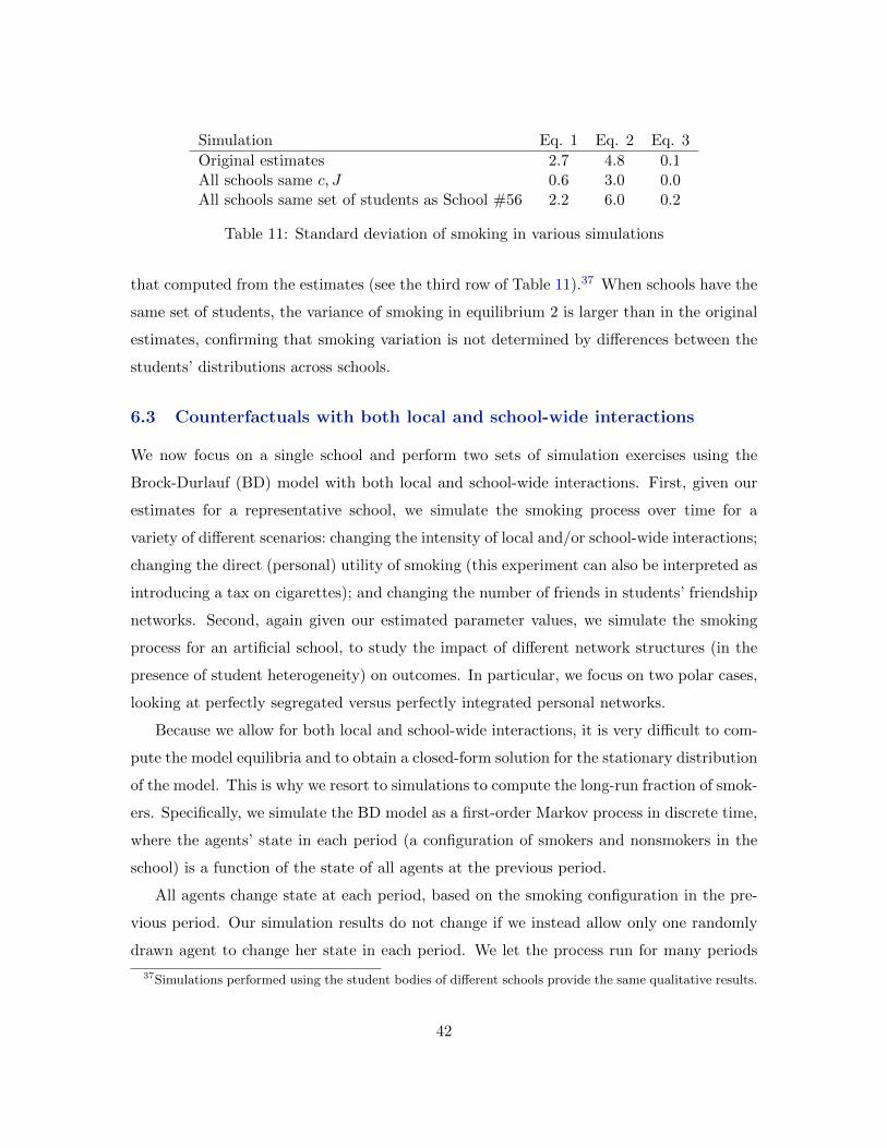
Simulation Eq. 1 Eq. 2 Eq. 3

Original estimates 2.7 4.8 0.1All schools same c, J 0.6 3.0 0.0All schools same set of students as School #56 2.2 6.0 0.2

Table 11: Standard deviation of smoking in various simulations

that computed from the estimates (see the third row of Table 11).37 When schools have the

same set of students, the variance of smoking in equilibrium 2 is larger than in the original

estimates, confirming that smoking variation is not determined by differences between the

students’ distributions across schools.

6.3 Counterfactuals with both local and school-wide interactions

We now focus on a single school and perform two sets of simulation exercises using the

Brock-Durlauf (BD) model with both local and school-wide interactions. First, given our

estimates for a representative school, we simulate the smoking process over time for a

variety of different scenarios: changing the intensity of local and/or school-wide interactions;

changing the direct (personal) utility of smoking (this experiment can also be interpreted as

introducing a tax on cigarettes); and changing the number of friends in students’ friendship

networks. Second, again given our estimated parameter values, we simulate the smoking

process for an artificial school, to study the impact of different network structures (in the

presence of student heterogeneity) on outcomes. In particular, we focus on two polar cases,

looking at perfectly segregated versus perfectly integrated personal networks.

Because we allow for both local and school-wide interactions, it is very difficult to com-

pute the model equilibria and to obtain a closed-form solution for the stationary distribution

of the model. This is why we resort to simulations to compute the long-run fraction of smok-

ers. Specifically, we simulate the BD model as a first-order Markov process in discrete time,

where the agents’ state in each period (a configuration of smokers and nonsmokers in the

school) is a function of the state of all agents at the previous period.

All agents change state at each period, based on the smoking configuration in the pre-

vious period. Our simulation results do not change if we instead allow only one randomly

drawn agent to change her state in each period. We let the process run for many periods

37Simulations performed using the student bodies of different schools provide the same qualitative results.

42

Percentage of smokers in low-level equilibrium

Local interaction parameter

0.2J0.5J0.8J0.9J

0.95J0.99J

J1.01J1.05J1.1J1.2J1.5J

2J3J

0.1J0.05J

0

5 10 15 20 25 30 1000Initial percentage of smokers

1.5

00.03

0.090.120.130.150.160.160.160.180.200.240.47

0.941.221.39

WLength of line represents thebasin of attraction of low-level equilibrium

U

Figure 7: Percentage of smokers and basins of attraction of low-level equilibrium in a repre-sentative school for different values of the local interaction parameter (high-level equilibriumis at 100 percent smokers in every simulation)

(2,400) and report the long-run average out of the last 1,000 iterations (we have also let

the process run for up to 10,000 periods as a robustness check; the reported results do not

change). We use the parameter estimates from the model specification with random coef-

ficients (no school covariates zn) and both local and school-wide interactions, as a parallel

to the specification we use for the counterfactuals with school-wide interactions only.38

6.3.1 Results for a representative school

We chose school #56 as a representative school, in terms of both its demographics and its

parameter estimates. Figures 7-11 report the results of our counterfactual experiments to

show the importance of multiple equilibria and nonlinearities. Figure 7 reports the equilibria

we find for several values of the local interactions parameter (displayed in the vertical axis).

The horizontal lines display the basin of attraction of the low-level equilibrium. For example,

at the estimated value of J, when setting an initial fraction of smokers between 0 and about

38We have also performed all counterfactual exercises using parameter estimates from other specifications.The results are qualitatively very similar.

43

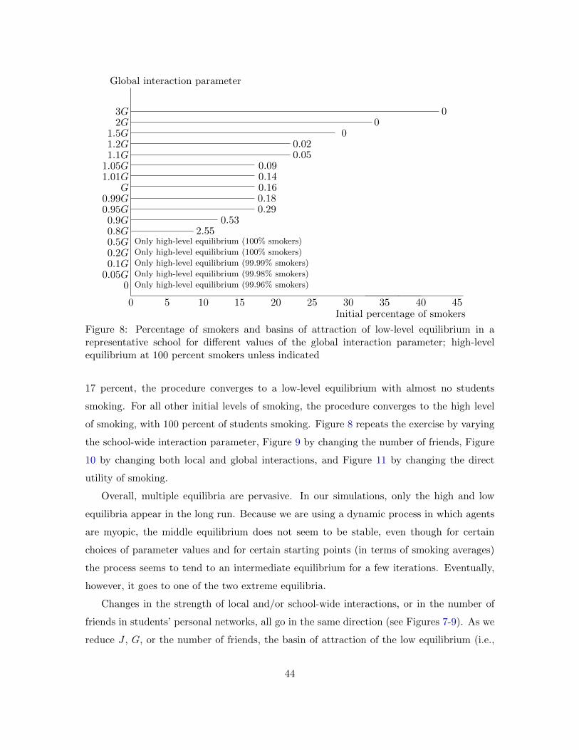
0.290.180.160.140.09

Global interaction parameter

0.2G0.5G0.8G0.9G

0.95G0.99G

G1.01G1.05G1.1G1.2G1.5G

2G3G

0.1G0.05G

0

5 10 15 20 25 30 35 40 450Initial percentage of smokers

Only high-level equilibrium (99.96% smokers)

Only high-level equilibrium (99.98% smokers)

Only high-level equilibrium (99.99% smokers)

Only high-level equilibrium (100% smokers)

Only high-level equilibrium (100% smokers)

0.53

00

0

0.020.05

2.55

Figure 8: Percentage of smokers and basins of attraction of low-level equilibrium in arepresentative school for different values of the global interaction parameter; high-levelequilibrium at 100 percent smokers unless indicated

17 percent, the procedure converges to a low-level equilibrium with almost no students

smoking. For all other initial levels of smoking, the procedure converges to the high level

of smoking, with 100 percent of students smoking. Figure 8 repeats the exercise by varying

the school-wide interaction parameter, Figure 9 by changing the number of friends, Figure

10 by changing both local and global interactions, and Figure 11 by changing the direct

utility of smoking.

Overall, multiple equilibria are pervasive. In our simulations, only the high and low

equilibria appear in the long run. Because we are using a dynamic process in which agents

are myopic, the middle equilibrium does not seem to be stable, even though for certain

choices of parameter values and for certain starting points (in terms of smoking averages)

the process seems to tend to an intermediate equilibrium for a few iterations. Eventually,

however, it goes to one of the two extreme equilibria.

Changes in the strength of local and/or school-wide interactions, or in the number of

friends in students’ personal networks, all go in the same direction (see Figures 7-9). As we

reduce J , G, or the number of friends, the basin of attraction of the low equilibrium (i.e.,

44

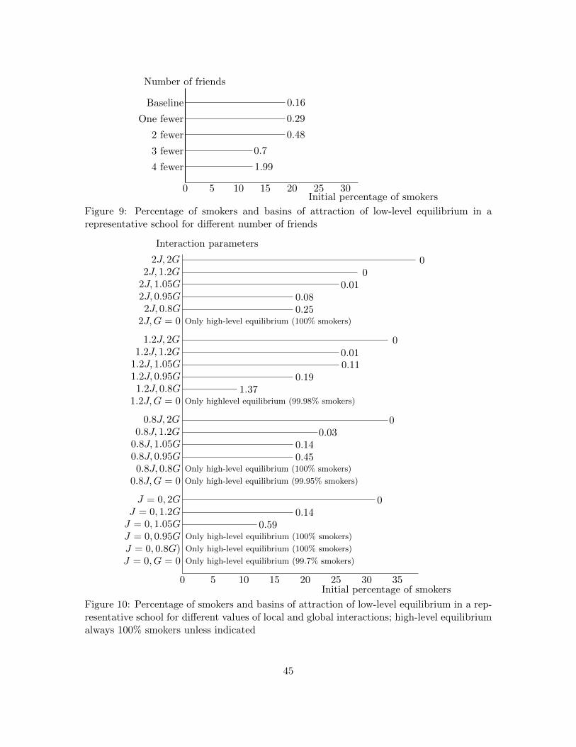
3 fewer

2 fewer

One fewer

Baseline

5 10 15 20 25 300Initial percentage of smokers

Number of friends

4 fewer 1.99

0.7

0.48

0.29

0.16

Figure 9: Percentage of smokers and basins of attraction of low-level equilibrium in arepresentative school for different number of friends

1.2J, 0.8G1.2J, 0.95G

1.2J, 1.2G1.2J, 2G

2J,G = 0

2J, 1.05G

Only high-level equilibrium (100% smokers)

2J, 0.8G2J, 0.95G

2J, 1.2G2J, 2G

0.140.59

0.450.14

0.191.37

0.110.01

0.250.08

0.01

0

00

Interaction parameters

J = 0, 0.95G

J = 0, 2G

0.8J,G = 0

0.8J, 1.05G

5 10 15 20 25 300Initial percentage of smokers

Only high-level equilibrium (100% smokers)

35

J = 0, G = 0 Only high-level equilibrium (99.7% smokers)

J = 0, 0.8G) Only high-level equilibrium (100% smokers)

J = 0, 1.2G

1.2J,G = 0

1.2J, 1.05G

Only highlevel equilibrium (99.98% smokers)

J = 0, 1.05G

0

Only high-level equilibrium (99.95% smokers)

Only high-level equilibrium (100% smokers)0.8J, 0.8G0.8J, 0.95G

0.030.8J, 1.2G0.8J, 2G 0

Figure 10: Percentage of smokers and basins of attraction of low-level equilibrium in a rep-resentative school for different values of local and global interactions; high-level equilibriumalways 100% smokers unless indicated

45

Ci − 0.5med(C)Ci − 0.2med(C)

Ci −med(C)Ci −max(C)

Ci = 0

10 20 30 400Initial percentage of smokers

Ci − 0.1med(C)Ci − 0.05med(C)Ci + 0.05med(C)Ci + 0.1med(C)Ci + 0.2med(C)Ci + 0.5med(C)

PPPqCi +med(C)Ci + 2med(C)

Only high-level equilibrium (100% smokers)

Utility from smoking

-

0.220.3

0.120.14

0.090.04

0

0.01

0.86

0

0.19

Figure 11: Percentage of smokers and basins of attraction of low-level equilibrium in arepresentative school for different values of direct utility from smoking

the set of initial conditions from which the process reaches it) shrinks, until it eventually

disappears; this is consistent with the left panel of Figure 6 (which illustrates movements in

the equilibrium mapping following a change in G). The fraction of smokers increases slightly

at the low equilibrium, until it jumps to a near totality of smokers in the high equilibrium

when the low equilibrium disappears. Local and school-wide interactions appear to be

“strategic complements” (Figure 10): Keeping the strength of local (respectively, school-

wide) interactions fixed, the basin of attraction of the low equilibrium shrinks as the strength

of school-wide (respectively, local) interactions decreases, and vice versa.39

Therefore, as is the case for school-wide only interactions, a decrease in the magnitude

of social interactions leads, in a very nonlinear fashion, to a sharp increase in the prevalence

of smoking in the representative school. For low levels of social interactions, only the high

equilibrium survives, in which almost every student smokes. This confirms the observation

made earlier: that the presence of social interactions may actually lead to lower equilibrium

smoking than would be the case in their absence.

Figure 11 reports the effect of changes in the individual cost of cigarettes (measured

in “utils”): Specifically, a decrease in the cost of smoking is modeled as an increase of the

intercept in the random utility of smoking of each student. This experiment changes the

39When school-wide interactions (G) are set to zero and only local interactions (J) are present, multipleequilibria persist for sufficiently large values of J (not reported here).

46

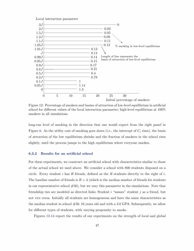
0.210.170.150.140.140.13

0.05

Length of line represents thebasin of attraction of low-level equilibrium

% smoking in low-level equilibrium

Local interaction parameter

0.2J0.5J0.8J0.9J

0.95J0.99J

J1.01J1.05J1.1J1.2J1.5J

2J3J

0.1J0.05J

0

5 10 15 20 25 300Initial percentage of smokers

0.09

0

R

W

1.31.141

0.780.4

0.110.12

0.02

Figure 12: Percentage of smokers and basins of attraction of low-level equilibrium in artificialschool for different values of the local interaction parameter; high-level equilibrium at 100%smokers in all simulations

long-run level of smoking in the direction that one would expect from the right panel in

Figure 6. As the utility cost of smoking goes down (i.e., the intercept of Ci rises), the basin

of attraction of the low equilibrium shrinks and the fraction of smokers in the school rises

slightly, until the process jumps to the high equilibrium where everyone smokes.

6.3.2 Results for an artificial school

For these experiments, we construct an artificial school with characteristics similar to those

of the actual school we used above. We consider a school with 800 students disposed on a

circle. Every student i has R friends, defined as the R students directly to the right of i.

The baseline number of friends is R = 4 (which is the median number of friends for students

in our representative school #56), but we vary this parameter in the simulations. Note that

friendship ties are modeled as directed links: Student i “names” student j as a friend, but

not vice versa. Initially all students are homogeneous and have the same characteristics as

the median student in school #56: 16 years old and with a 3.0 GPA. Subsequently, we allow

for different types of students, with varying propensity to smoke.

Figures 12-14 report the results of our experiments on the strength of local and global

47

0.240.150.14

Global interaction parameter

0.2G0.5G0.8G0.9G

0.95G0.99G

G1.01G1.05G1.1G1.2G1.5G

2G3G

0.1G0.05G

0

5 10 15 20 25 300Initial percentage of smokers

Only highlevel equilibrium (99.97% smokers)

Only high-level equilibrium (99.98% smokers)

Only high-level equilibrium (99.99% smokers)

Only high-level equilibrium (99.99% smokers)

Only high-level equilibrium (100% smokers)

0

35

0.080.05

0.02

0.12

1.660.43

00

Figure 13: Percentage of smokers and basins of attraction of low-level equilibrium in artificialschool for different values of the global interaction parameter; high-level equilibrium at 100%smokers unless indicated

interactions (changes in J,G) and on the number of friends R. The artificial school behaves

very similarly to the representative one. Reductions in local interactions J, in school-wide

interactions G, or in the number of friends R all induce the basin of attraction of the

low equilibrium to become smaller and eventually disappear. While the low equilibrium

persists, reductions in these parameters are associated with a slight increase in the fraction

of smokers in the school. As with the actual school, holding fixed any two parameters

in (J,G,R) while reducing the third one has the same qualitative effect on the basin of

attraction of the low equilibrium and on the fraction of smokers in this equilibrium while

it persists. Thus, as in the representative school case, stronger social interactions and/or a

larger number of friends tend to reduce smoking, according to our estimates.

Figure 15 reports the effects of changing the demographic characteristics of all artificial

students in the school; agents are still homogeneous here. These experiments are equivalent

to shifting the intercept of the individual utility of smoking (conceptually, it is the same as

introducing a “tax/subsidy” on cigarettes). For younger students, or those with a higher

GPA, the intercept shifts down relative to our baseline student, which induces the basin of

48

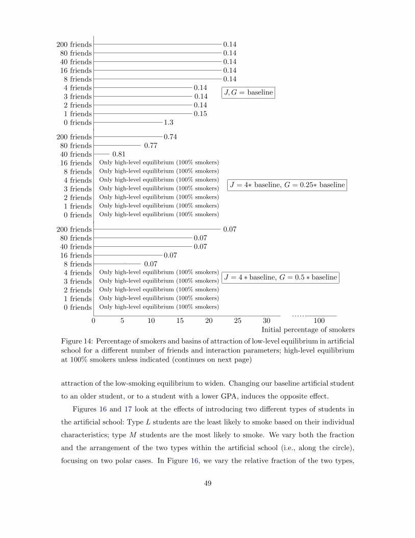
5 10 15 20 25 30 1000Initial percentage of smokers

Only high-level equilibrium (100% smokers)0 friends1 friends2 friends3 friends4 friends8 friends

16 friends40 friends80 friends

200 friends

J,G = baseline

J = 4 ∗ baseline, G = 0.5 ∗ baseline

Only high-level equilibrium (100% smokers)0 friends1 friends2 friends3 friends4 friends8 friends

16 friends40 friends80 friends

200 friends

J = 4∗ baseline, G = 0.25∗ baseline

Only high-level equilibrium (100% smokers)

Only high-level equilibrium (100% smokers)

Only high-level equilibrium (100% smokers)

Only high-level equilibrium (100% smokers)

0 friends1 friends2 friends3 friends4 friends8 friends

16 friends40 friends

0.140.15

0.14

0.1480 friends 0.14

200 friends 0.14

Only high-level equilibrium (100% smokers)

Only high-level equilibrium (100% smokers)

0.07

Only high-level equilibrium (100% smokers)

Only high-level equilibrium (100% smokers)

0.07

0.070.07

1.3

0.07

0.140.14

0.14

0.74

0.81

Only high-level equilibrium (100% smokers)

Only high-level equilibrium (100% smokers)

0.77

Figure 14: Percentage of smokers and basins of attraction of low-level equilibrium in artificialschool for a different number of friends and interaction parameters; high-level equilibriumat 100% smokers unless indicated (continues on next page)

attraction of the low-smoking equilibrium to widen. Changing our baseline artificial student

to an older student, or to a student with a lower GPA, induces the opposite effect.

Figures 16 and 17 look at the effects of introducing two different types of students in

the artificial school: Type L students are the least likely to smoke based on their individual

characteristics; type M students are the most likely to smoke. We vary both the fraction

and the arrangement of the two types within the artificial school (i.e., along the circle),

focusing on two polar cases. In Figure 16, we vary the relative fraction of the two types,

49

5 10 15 20 25 30 350Initial percentage of smokers

0 friends1 friends2 friends3 friends4 friends8 friends

16 friends40 friends80 friends

200 friends

00

000

J = 8∗baseline, G = baseline

0 friends1 friends2 friends3 friends4 friends8 friends

16 friends40 friends80 friends

200 friends

0.01

J = 4∗baseline, G = baseline

0

00

01.29

0000

000

0

1.29

Figure 14: (continued) Percentage of smokers and basins of attraction of low-level equilib-rium in artificial school for different number of friends and interaction parameters; high-levelequilibrium at 100% smokers unless indicated

Least

5 10 15 20 25 300Initial percentage of smokers

>

13yo, GPA = 4Baseline

:

1

16yo, GPA=3

19yo, GPA=2

Most 0.7

0.13

0.03

Figure 15: Percentage of smokers and basins of attraction of low-level equilibrium in artificialschool for different artificial (homogenous) students; high-level equilibrium at 100% smokersunless indicated

50

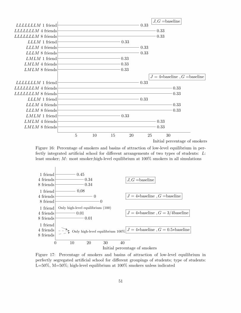
5 10 15 20 25 30

Initial percentage of smokers

J,G =baseline

LMLM 8 friends

LMLM 4 friends

LMLM 1 friend

LLLM 8 friends

LLLM 4 friends

LLLM 1 friend

LLLLLLLM 8 friends

LLLLLLLM 4 friends

LLLLLLLM 1 friend

LMLM 8 friends

LMLM 4 friends

LMLM 1 friend

LLLM 8 friends

LLLM 4 friends

LLLM 1 friend

LLLLLLLM 8 friends

LLLLLLLM 4 friends

LLLLLLLM 1 friend

0.33

0.33

0.33

0.33

0.33

0.33

0.33

0.33

0.33

0.33

0.33

0.33

0.33

0.33

0.33

0.33

0.33

0.33

J = 4∗baseline , G =baseline

Figure 16: Percentage of smokers and basins of attraction of low-level equilibrium in per-fectly integrated artificial school for different arrangements of two types of students: L:least smoker; M : most smoker;high-level equilibrium at 100% smokers in all simulations

10 20 30 400Initial percentage of smokers

1 friend4 friends8 friends

1 friend4 friends8 friends

1 friend4 friends8 friend

1 friend4 friends8 friends

J,G =baseline

J = 4∗baseline , G =baseline

J = 4∗baseline , G = 3/4baseline

J = 4∗baseline , G = 0.5∗baselineOnly high-level equilibrium 100%q-:

0.45

0.340.34

0

0,08

0

0.01

Only high-level equilibrium (100)

0.01

Figure 17: Percentage of smokers and basins of attraction of low-level equilibrium inperfectly segregated artificial school for different groupings of students; type of students:L=50%, M=50%; high-level equilibrium at 100% smokers unless indicated

51

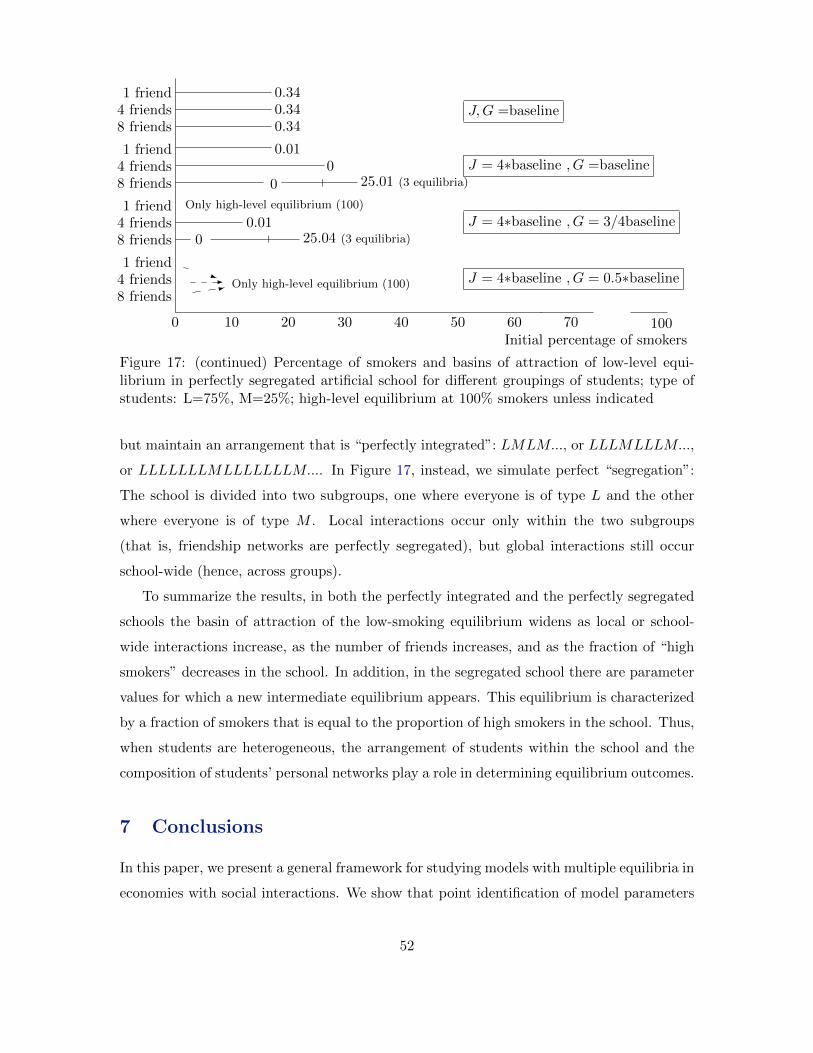
10 20 30 40 50 600Initial percentage of smokers

70 100

1 friend4 friends8 friends

1 friend4 friends8 friends

1 friend4 friends8 friends

1 friend4 friends8 friends

J,G =baseline

J = 4∗baseline , G =baseline

J = 4∗baseline , G = 3/4baseline

J = 4∗baseline , G = 0.5∗baselineOnly high-level equilibrium (100)q-:

Only high-level equilibrium (100)

0.340.34

0.01

0.34

00.01

0 25.04 (3 equilibria)

0 25.01 (3 equilibria)

Figure 17: (continued) Percentage of smokers and basins of attraction of low-level equi-librium in perfectly segregated artificial school for different groupings of students; type ofstudents: L=75%, M=25%; high-level equilibrium at 100% smokers unless indicated

but maintain an arrangement that is “perfectly integrated”: LMLM..., or LLLMLLLM...,

or LLLLLLLMLLLLLLLM.... In Figure 17, instead, we simulate perfect “segregation”:

The school is divided into two subgroups, one where everyone is of type L and the other

where everyone is of type M . Local interactions occur only within the two subgroups

(that is, friendship networks are perfectly segregated), but global interactions still occur

school-wide (hence, across groups).

To summarize the results, in both the perfectly integrated and the perfectly segregated

schools the basin of attraction of the low-smoking equilibrium widens as local or school-

wide interactions increase, as the number of friends increases, and as the fraction of “high

smokers” decreases in the school. In addition, in the segregated school there are parameter

values for which a new intermediate equilibrium appears. This equilibrium is characterized

by a fraction of smokers that is equal to the proportion of high smokers in the school. Thus,

when students are heterogeneous, the arrangement of students within the school and the

composition of students’ personal networks play a role in determining equilibrium outcomes.

7 Conclusions

In this paper, we present a general framework for studying models with multiple equilibria in

economies with social interactions. We show that point identification of model parameters

52

is conceptually distinct from the presence of multiple equilibria, and derive some general

conditions for identification. We then present a two-step estimation strategy that, while

less efficient than the direct maximum-likelihood estimator, has two significant advantages.

First, it is computationally feasible, as it is several orders of magnitude faster than the direct

or the Dagsvik-Jovanovic method; second, it does not rely on making explicit assumptions

about the nature of the selection mechanism across equilibria, as in the D-J method.

We then apply our estimation approach to a version of the Brock-Durlauf binary choice

model with social interactions, using data on teenage smoking. We find statistically signif-

icant evidence of both school-wide and local (within personal networks) interactions. Our

estimates are consistent across specifications that take into account school and local neigh-

borhood attributes. Given our estimates, multiple equilibria are prevalent in our data: the

estimated parameter values give rise to multiplicity in forty out of forty-one schools. In

many cases where multiple equilibria are present, there exists one other equilibrium with a

lower smoking prevalence than that observed in a given school.

Having estimated the parameters of a structural model, we are able to run several

counterfactual experiments. In specifications with school-wide interactions only, we show

that reductions in the strength of social interactions may increase or decrease smoking

prevalence, depending on whether the school is in the low or intermediate equilibrium. Large

reductions in school-wide interactions eventually make equilibrium multiplicity disappear,

with only the high smoking equilibrium surviving. Thus, tobacco policies that are associated

with lower school-wide social interactions may have the counterintuitive and undesirable

effect of actually increasing smoking prevalence in a school, sometimes by a large amount.

Simulations in settings where both school-wide and local interactions are present show

that reductions in local and/or global interactions, or in the number of friends, make the

basin of attraction of the low-smoking equilibrium shrink until it disappears; while this

equilibrium persists, smoking prevalence rises slightly. Reductions in the utility cost of

smoking also make the basin of attraction of low equilibria become smaller, and smoking

prevalence increases. When the low equilibrium disappears, the fraction of smokers in a

school jumps dramatically to an equilibrium where almost everyone smokes. Finally, the

arrangement of students within a school, and hence the structure of personal networks

(e.g., segregation versus integration by demographics), can influence the number and types

53

of smoking equilibria that may arise.

These results should be taken as an illustration of the kind of policy experiments that

one may carry out after having obtained structural parameter estimates for a behavioral

model of smoking with social interactions that exhibits multiple equilibria. However, they

should not be taken literally: here, we assume that personal networks are given and that

tobacco use policies are exogenous, the model does not incorporate dynamic features such

as addiction, and we do not take a stand on the way in which agents select a specific

equilibrium. This is left for future work. In a companion paper (Bisin, Moro, and Topa (in

progress)), we study settings where friendship networks are endogenous. Agents sort on the

basis of both observable and unobservable attributes, which in turn may be related to one’s

propensity to smoke. Taking this endogeneity explicitly into account can help identify the

extent of social interactions.

A Appendix: Regularity assumptions on general societies

and proofs of propositions

In this appendix, we detail the construction of general societies in Section 2, as well as our

analysis of identification and estimation in Sections 3 and 4. We also sketch the proofs of

Propositions 1-3, that depend on this construction. While assumptions are overly strong in

several dimensions, it is left for a separate paper to obtain tighter conditions.

A.1 First-order conditions

Let agent i’s maximization problem be:

maxyi∈Y

V(yi, xi,yg(i), πn, εi, zn, un

).

Let Pi(y, x | yg(i), πn, zn, un

)denote the first-order conditions of the problem.

We assume that Pi(y, x | yg(i), πn, zn, un

)is continuous and differentiable, for any i.

This is guaranteed if either

(i) the choice set Y is convex and compact, the utility function V(yi, xi,yg(i), πn, εi, zn, un

)is C2 in its arguments and Inada conditions to avoid corner solutions are imposed,

54

the density p(εi | zn, un) is non-atomic and C2 as a function of (zn, un); or

(ii) the choice set Y is discrete, the utility function V(yi, xi,yg(i), πn, εi, zn, un

)is C2 in

its arguments for any yi ∈ Y , the density p(εi | zn, un) is non-atomic and C2 as a

function of (zn, un).

We also assume that Pi(y, x | yg(i), πn, zn, un

)is strictly positive.

A.2 The probability distribution P (yn,xn | πn, zn, un)

Recall that, at an equilibrium in sub-population n, given πn, there exists an ergodic proba-

bility distribution on the configuration of actions and characteristics (yn,xn), P (yn,xn | πn, zn, un)

such that

P(yi = y, xi = x | yg(i), πn, zn, un

)= Pi

(y, x | yg(i), πn, zn, un

), P − a.s.,

Existence of such a P (yn,xn | πn, zn, un) is guaranteed if the probability distribution

Pi(y, x | yg(i), πn, zn, un

)has a Markovian structure across agents i; for the proof of this

statement, see Follmer (1974), Section 3, and Preston (2008). In our context, this in turn

is essentially guaranteed by the assumption that | g(i) |< ∞ for any i. More precisely,

existence also requires a weak homogeneity condition on the network structure implied by

the map g; e.g., translation invariance on a lattice is sufficient; see Follmer (1974) and Horst

and Scheinkman (2006). This assumption is always satisfied in the examples and we avoid

making it formally explicit.

To guarantee that the probability distribution P (yn,xn | πn, zn, un) is ergodic (and that

it preserves the homogeneity property) it is sufficient that preferences in society satisfy a

Moderate Social Influence condition,40 which bounds the strength of the local interactions.

In the case Y is a continuous space, for instance, these conditions require, for any j ∈ g(i),

that | ∂V (yi,xiyg(i),πn,εi,zn,un)∂yj

| has a uniform (in the arguments of V ) and small enough

bound k; see Horst and Scheinkman (2006), Theorem 19 (ii).

Uniqueness of such a P (yn,xn | πn, zn, un) requires a stronger Moderate Social Influence

condition, e.g., bounding the∑

j∈g(i) |∂V (yi,xiyg(i),πn,εi,zn,un)

∂yj|; see Horst and Scheinkman

40Such conditions, and the associated terminology, have been introduced by Glaeser and Scheinkman(2001, 2003).

55

(2006), Theorem 19 (iii). Furthermore, a straightforward extension of Theorem 3.1.2 in

Follmer (1974) to our context implies that uniqueness is also guaranteed if the network

induced by the map g is one-dimensional; that is, if agents i ∈ In can, without loss of

generality, be disposed on a line.

Ergodicity of P (yn,xn | πn, zn, un) implies that

lim|In|→∞

1

|In|∑i∈In

A (yi, xi, πn, zn, un) = EP [A (yi, xi, πn, zn, un)] , for any i ∈ In,

so that πn is well defined; in particular, if

πn = lim|In|→∞

1

|In|∑i∈In

yi.

More generally, existence of πn requires e.g., the standard boundary conditions onA (yi, xi, πn, zn, un)

which are typically satisfied by excess demand functions in general equilibrium theory; see

e.g., Mas Colell, Whinston, and Green (1995), Chapter 17, C, D.

A.3 The correspondence L(y,x | z;θ)

Recall that

L(y,x | z;θ) =

∫[Πn∈NP(zn, un; θn)] p (u) du

where P(zn, un; θn) = P(πn(zn, un; θeqn ), zn, un; θfocn ) and∫

denotes the Aumann integral,

since P(zn, un; θn) is a correspondence. The Aumann integral is constructed by taking

the union of the Riemann integrals of all measurable selections of the correspondence; it

coincides with the Riemann integral when applied to a measurable function; see Aumann

(1965) and Molchanov (2005) for details.

A.4 Proofs

Proof of Proposition 1. It is straightforward to check that the conditions in Proposition

1 guarantee identification.

If P(πn, zn, un; θfocn ) maps (πn, un, θfocn ) onto P

(yn,xn | πn, zn, un; θfocn

), the inverse

56

map from P(yn,xn | πn, zn, un; θfocn

)to (πn, un, θ

focn ) is one-to-one. Therefore, given zn,

(πn, un,θfocn ) 6= (π′n, u

′n, θ

foc′n )⇒ P

(yn,xn | πn, zn, un;θfocn

)6= P

(yn,xn | π′n, zn, u′n;θfoc′n

).

Moreover, If πn(θeqn , zn, un) maps (θeqn , un) onto πn (given zn), then the inverse map from

πn into (θeqn , un) is one-to-one.

As a consequence, then

(θn, un) 6= (θ′n, u′n)⇒ P (yn,xn | zn, un;θn) 6= P

(yn,xn | zn, u′n;θ′n

),

and hence identification is satisfied.

Furthermore, conditions for the non-parametric identification of p(u), from the obser-

vation of un, for all n ∈ N , can be obtained as an application of the previously cited results

on interacting systems of conditional probabilities in Follmer (1974), Section 3, and Preston

(2008). In particular, it is required that the process un has a Markovian (and homogeneous)

structure across populations n ∈ N and that it satisfies Moderate Social Influence condi-

tions.

Proof of Proposition 2. Under our assumptions the correspondenceL(y,x | z;θ) is

compact valued and measurable selections are non-atomic. It follows that the set induced

by Aumann integration, L(z;θ), is compact.

Consider now the problem maxl(y,x|z;θ)∈L(z;θ) l(y,x|z;θ) Because of compactness of

L(z;θ) a maximum exists and the argmax is a upper-semi-continuous function of θ.

Consistency of the maximum-likelihood estimator (for an identified set of parameters)

now follows along the standard path of arguments: i) the strong Law of Large Numbers

in fact holds for upper-semi-continuous functions; see Lebanon (2008), Proposition 1 (from

Ferguson, 1996, Theorem 16(a); and non-negativity of the KL divergence applies to arbitrary

densities (see Lebanon (2008)).

The Proof of Proposition 3 is straightforward. Consistency of the second step, given

πn P , does not require any extension of the standard result for maximum-likelihood esti-

mators. As long as πn and P are estimated consistently, then θn will be as well.

57

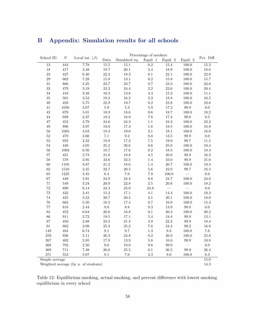
B Appendix: Simulation results for all schools

School ID N Local int. (J)Percentage of smokers

Pct. Diff.Data Simulated eq. Equil. 1 Equil. 2 Equil. 3

13 444 7.78 15.5 15.1 0.2 15.4 100.0 15.3

18 417 3.48 19.7 20.1 2.4 18.9 100.0 16.6

23 427 6.40 22.2 18.3 0.1 22.1 100.0 22.0

29 602 7.28 15.9 13.1 0.2 15.8 100.0 15.7

31 866 4.25 23.7 23.7 0.7 23.3 100.0 22.6

33 479 3.19 23.2 24.4 2.2 22.6 100.0 20.4

34 418 3.48 16.3 13.6 4.3 15.3 100.0 11.1

35 501 3.52 19.2 16.2 2.3 18.8 100.0 16.5

40 458 5.75 22.9 19.7 0.2 22.8 100.0 22.6

41 1056 2.67 5.9 5.3 5.9 17.2 99.9 0.0

42 679 5.01 18.9 18.6 0.6 18.7 100.0 18.2

44 939 2.37 18.2 16.9 7.8 17.3 99.8 9.5

47 452 3.79 24.6 24.3 1.1 24.2 100.0 23.2

49 896 3.97 19.0 17.3 1.6 18.5 100.0 16.9

50 1085 3.63 18.3 19.0 2.1 18.1 100.0 16.0

52 479 2.66 7.1 9.2 8.0 13.5 99.9 0.0

53 935 2.32 19.8 17.2 7.5 19.0 99.7 11.5

54 448 4.05 25.2 26.6 0.6 25.0 100.0 24.4

56 1093 6.50 18.7 17.6 0.2 18.5 100.0 18.3

57 421 2.73 21.6 18.8 4.5 20.8 99.9 16.3

58 578 2.95 33.6 32.5 1.4 33.0 99.9 31.6

60 1105 3.87 21.2 18.6 1.4 20.7 100.0 19.3

62 1510 2.45 22.7 20.5 5.6 22.0 99.7 16.4

65 1225 3.45 6.4 7.0 7.9 100.0 — 0.0

67 449 3.91 24.9 24.3 0.8 24.7 100.0 24.0

71 549 3.24 20.9 22.8 2.5 20.6 100.0 18.2

72 899 0.14 24.4 25.0 24.8 — — 0.0

73 422 3.41 15.2 17.1 4.1 14.4 100.0 10.3

74 435 3.53 20.7 20.5 2.1 20.1 100.0 18.0

76 662 5.50 16.2 17.4 0.7 16.0 100.0 15.3

77 818 2.44 9.0 8.8 9.3 13.9 99.8 0.0

82 452 6.64 20.6 16.8 0.1 20.3 100.0 20.2

86 911 2.72 19.5 17.1 5.4 18.4 99.9 13.1

87 450 2.88 23.3 21.3 3.9 22.2 99.9 18.4

91 862 2.09 25.3 25.2 7.6 24.4 99.2 16.8

149 484 6.74 9.1 9.7 1.3 8.8 100.0 7.6

259 936 5.11 26.3 24.8 0.2 26.0 100.0 25.8

267 402 2.85 17.9 13.9 5.8 16.6 99.9 10.8

268 792 2.50 9.6 10.0 9.8 99.9 — 0.0

269 711 7.48 26.6 25.5 0.1 26.5 99.9 26.4

271 552 5.67 9.1 7.6 2.3 8.6 100.0 6.3

Simple average 15.0

Weighted average (by n. of students) 14.3

Table 12: Equilibrium smoking, actual smoking, and percent difference with lowest smokingequilibrium in every school

58

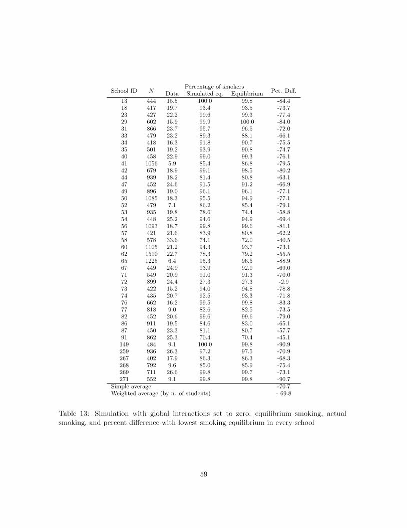
School ID NPercentage of smokers

Pct. Diff.Data Simulated eq. Equilibrium13 444 15.5 100.0 99.8 -84.418 417 19.7 93.4 93.5 -73.723 427 22.2 99.6 99.3 -77.429 602 15.9 99.9 100.0 -84.031 866 23.7 95.7 96.5 -72.033 479 23.2 89.3 88.1 -66.134 418 16.3 91.8 90.7 -75.535 501 19.2 93.9 90.8 -74.740 458 22.9 99.0 99.3 -76.141 1056 5.9 85.4 86.8 -79.542 679 18.9 99.1 98.5 -80.244 939 18.2 81.4 80.8 -63.147 452 24.6 91.5 91.2 -66.949 896 19.0 96.1 96.1 -77.150 1085 18.3 95.5 94.9 -77.152 479 7.1 86.2 85.4 -79.153 935 19.8 78.6 74.4 -58.854 448 25.2 94.6 94.9 -69.456 1093 18.7 99.8 99.6 -81.157 421 21.6 83.9 80.8 -62.258 578 33.6 74.1 72.0 -40.560 1105 21.2 94.3 93.7 -73.162 1510 22.7 78.3 79.2 -55.565 1225 6.4 95.3 96.5 -88.967 449 24.9 93.9 92.9 -69.071 549 20.9 91.0 91.3 -70.072 899 24.4 27.3 27.3 -2.973 422 15.2 94.0 94.8 -78.874 435 20.7 92.5 93.3 -71.876 662 16.2 99.5 99.8 -83.377 818 9.0 82.6 82.5 -73.582 452 20.6 99.6 99.6 -79.086 911 19.5 84.6 83.0 -65.187 450 23.3 81.1 80.7 -57.791 862 25.3 70.4 70.4 -45.1149 484 9.1 100.0 99.8 -90.9259 936 26.3 97.2 97.5 -70.9267 402 17.9 86.3 86.3 -68.3268 792 9.6 85.0 85.9 -75.4269 711 26.6 99.8 99.7 -73.1271 552 9.1 99.8 99.8 -90.7

Simple average -70.7Weighted average (by n. of students) - 69.8

Table 13: Simulation with global interactions set to zero; equilibrium smoking, actualsmoking, and percent difference with lowest smoking equilibrium in every school

59

References

Aguirregabiria, V. (2004): ”Pseudo Maximum Likelihood Estimation of Structural Models

Involving Fixed-Point Problems,” Economics Letters, 84(3), 335-40.

Aguirregabiria, V. and P. Mira (2007): “Sequential Estimation of Dynamic Discrete

Games,” Econometrica, 75(1), 1-53.

Aiyagari, S.R. (1995): ”Comments on Farmer and Guo’s ‘The Econometrics of Indetermi-

nacy: An Applied Study’,” Federal Reserve Bank of Minneapolis, Research Depart-

ment Staff Report 196.

Andrews, D.W.K., S.T. Berry, and P. Jia (2004): “Confidence Regions for Parameters

in Discrete Games with Multiple Equilibria, with an Application to Discount Chain

Store Location”, Yale University, mimeo.

Aumann, R.J. (1965): ”Integrals of Set Valued Functions,” Journal of Mathematical Anal-

ysis and Applications, 12, 1-12.

Bajari, P., H. Hong, and S. Ryan (2010): “Identification and Estimation of a Discrete

Game of Complete Information”, Econometrica, 78 (5), 1529-1568.

Bajari, P., L. Benkard, and J. Levin (2007): “Estimating Dynamic Models of Imperfect

Competition”, Econometrica, 75 (5), 1331-1370.

Bajari, P., H. Hong, J. Krainer, and D. Nekipelov (2006): “Estimating Static Models of

Strategic Interactions,” NBER Working Paper 12013.

Bauman, K. and L. Fisher (1986): “On the Measurement of Friend Behavior in Research

on Friend Influence and Selection: Findings from Longitudinal Studies of Adolescent

Smoking and Drinking,” Journal of Youth and Adolescence, 15, 345-53.

Benhabib, J. and R. Farmer (1999): “Indeterminacy and sunspots in macroeconomics,” in

J.B. Taylor and M. Woodford (eds.), Handbook of Macroeconomics, Vol. 1, 387-448.

Beresteanu, A., I. Molchanov, and F. Molinari (2008): “Sharp Identification Regions in

Games,” Cemmap working paper CWP15/08.

60

Berry, S.T. and E. Tamer (2007): ”Identification in Models of Oligopoly Entry,” in

Advances in Economics and Econometrics: Theory and Applications, Ninth World

Congress, vol. II, Chap. 2, 46-85, Cambridge: Cambridge University Press.

Bisin, A., A. Moro and G. Topa (in progress): “Social Interactions, Endogenous Networks

and Teenage Smoking”, mimeo.

Bisin, A., G. Topa and T. Verdier (2004): “Religious Intermarriage and Socialization in

the United States” Journal of Political Economy, Vol. 112 (3), 615-664.

Bjorn, P.A. and Q.H. Vuong (1985): “Simultaneous Equation Models for Dummy Endoge-

nous Variables: A Game Theoretic Formulation with an Application to Labor Force

Participation,” Caltech, Working Paper 537.

Blume, L.E., W.A. Brock, S.N. Durlauf and Y.M. Ioannides (2011): “Identification of

Social Interactions”, in Benhabib J., A. Bisin and M.O. Jackson (Eds.) Handbook of

Social Economics, Vol. 1B, Chapter 18, 853-964, Amsterdam: North Holland.

Blume, L. and S. Durlauf, (1998): “Equilibrium Concepts for Social Interaction Models,”

mimeo, Cornell University.

Blume, L. and S. Durlauf, (2001): “The Interactions-Based Approach to Socioeconomic

Behavior,” in S. Durlauf and P. Young (eds.), Social Dynamics, Brookings Institution

Press and MIT Press, Cambridge, MA.

Bramoulle’ Y., H. Djebbari and B. Fortin (2009): “Identification of Peer Effects through

Social Networks”, Journal of Econometrics, Vol. 150(1), pp. 41-55.

Bresnahan, T. F. and P. C. Reiss (1991): “Empirical Models of Discrete Games”, Journal

of Econometrics 64, 57-81.

Brock, W.A. and S. N. Durlauf (2001a): “Interaction-Based Models,” in J. J. Heckman

and E. E. Leamer, eds., Handbook of Econometrics, North-Holland, Chapter V.

Brock, W. and S. Durlauf (2001b): “Discrete Choice with Social Interactions”, The Review

of Economic Studies, 68, 235-260.

61

Brock, W. and S. Durlauf (2007): “Identification of Binary Choice Models with Social

Interactions,” Journal of Econometrics, 140, 52-75.

Calvo-Armengol, A., E. Patacchini, and Y. Zenou (2009): “Peer Effects and Social Net-

works in Education,” The Review of Economic Studies, forthcoming.

Ciliberto, F. and E. Tamer (2009): “Market Structure and Multiple Equilibria in Airline

Markets,” Econometrica, 77 (6), 1791-1828.

Conley, T.G. and G. Topa (2002): “Socio-Economic Distance and Spatial Patterns in

Unemployment ”, Journal of Applied Econometrics, Vol. 17 (4), 303-327.

Conley, T.G. and G. Topa (2007): “Estimating Dynamic Local Interactions Models”,

Journal of Econometrics, Vol. 140 (1), 282-303.

Crane, J. (1991): “The Epidemic Theory of Ghettoes and Neighborhood Effects of Drop-

ping Out and Teenage Childbearing,” American Journal of Sociology, 96, 1229-59.

Dagsvik, J. and B. Jovanovic (1994): “Was the Great Depression a Low-Level Equilib-

rium?” European Economic Review, 38, 1711-29.

Davezies, L., X. D’Haultfoeuille, and D. Fougere (2006): “Identification of Peer Effects

Using Group Size Variation,” CEPR Discussion Paper 5865.

De Giorgi, G., M. Pellizzari, and S. Redaelli (2010): “Identification of Social Interactions

through Partially Overlapping Peer Groups,” American Economic Journal: Applied

Economics, 2, 241-275.

Echenique, F. and I. Komunjer (2005): “Testing Models with Multiple Equilibria by Quan-

tile Methods,” California Institute of Technology Social Science Working Paper 1244.

Fang, H. (2006): “Disentangling the College Wage Premium: Estimating a Model with

Endogenous Education Choices,” International Economic Review, 47(4), 1151-1185.

Farmer, R. and J.-T. Guo (1995): “The Econometrics of Indeterminacy: An Applied

Study,” Carnegie-Rochester Series in Public Policy, 43, 225-272.

Ferguson, T.S. (1996): A Course in Large Sample Theory, New York, Chapman & Hall.

62

Follmer, H. (1974): “Random Economies with Many Interacting Agents,” Journal of Math-

ematical Economics, 1, 51-62.

Follmer, H. and U. Horst (2001): “Convergence of Locally and Globally Interacting Markov

Chains,” Stochastic Processes and their Applications, 96, 99-121.

Galichon, A. and M. Henry (2008): “Inference in Models with Multiple Equilibria,” Uni-

versite’ de Montreal, mimeo.

Gaviria, A. and S. Raphael (2001): “School-Based Peer Effects and Juvenice Behavior,”

Review of Economics and Statistics, 83(2), 257-68.

Gilleskie, D.B. and K.S. Strumpf (2005): “The Behavioral Dynamics of Youth Smoking”,

Journal of Human Resources, XL(4):822-866.

Glaeser, E. and J.A. Scheinkman (2001): “Measuring Social Interaction,” in S. Durlauf

and P. Young (eds.), Social Dynamics, Cambridge, MA: Brookings Institution Press

and MIT Press. (2001)

Glaeser, E. and J.A. Scheinkman (2003): “Nonmarket interactions,” in M. Dewatripont,

L.P. Hansen, S.J. Turnovsky (eds), Advances in Economics and Econometrics: The-

ory and Applications, Eighth World Congress 1: 339 - 369, Cambridge: Cambridge

University Press.

Glaeser, E., B. Sacerdote, and J. Scheinkman (1996): “Crime and Social Interactions,”

Quarterly Journal of Economics, CXI, 507-548.

Graham, B.S. and J. Hahn (2005): “Identification and Estimation of the Linear-in-Means

Model of Social Interactions,” Economics Letters, 88, 1-6.

Gruber, J. and J. Zinman (2000): “Youth Smoking in the U.S.: Evidence and Implica-

tions”, NBER Working Paper No. 7780, July 2000.

Head, K. and T. Mayer (2008): “Detection of Local Interactions from the Spatial Patterns

of Names in France,” Journal of Regional Science, 48(1), 67-95.

Horst, U. and H. Follmer (2001): “Convergence oflocally and globally interacting Markov

chains,” Stochastic Processes and their Applications, 96, 99121.

63

Imrohoroglu, S. (1993): “Testing for Sunspot Equilibria in the German Hyperinflation,”

Journal of Economics Dynamics and Control, 17(2), 289-317.

Ioannides, Y.M., and J.E. Zabel (2008): “Interactions, Neighborhood Selection and Hous-

ing Demand,” Journal of Urban Economics, 63, 229-252.

Ioannides, Y.M. and G. Zanella (2008): “Searching for the Best Neighborhood: Mobility

and Social Interactions,” mimeo, Tufts University.

Jones, A. (1994): “Health, Addiction, Social Interaction, and the Decision to Quit Smok-

ing,” Journal of Health Economics, 13, 93-110.

Jovanovic, B. (1989): “Observable Implications of Models with Multiple Equilibria,”,

Econometrica, 57, 1431-1437.

Judd, K.L. and C.-L. Su (2006): “Constrained Optimization Approaches to Estimation of

Structural Models,”mimeo, University of Chicago.

Krauth, B.V. (2006): “Simulation-Based Estimation of Peer Effects,” Journal of Econo-

metrics, 133, 243-71.

Krosnick, J. and C. Judd (1982): “Transitions in Social Influence in Adolescence: Who

Induces Cigarette Smoking,” Develomental Psychology, 81, 359-68.

Lebanon, G. (2008): “Consistency of the Maximum Likelihood Estimator, ”mimeo, Geor-

gia Tech.

Lee, L.f (2007): “Identification and Estimation of Econometric Models with Group Inter-

actions, Contextual Factors and Fixed Effects,” Journal of Econometrics, 140, 333-74.

Lehmann, E.L. and G. Casella (1998): Theory of Point Estimation, New York, Springer.

Manski, C.F. (1993): “Identification of Endogenous Social Effects: The Reflection Prob-

lem”, Review of Economic Studies, 60 (3), 531-542.

Manski, C.F. and E. Tamer (2002): “Inference on Regressions with Interval Data on a

Regressor or Outcome,” Econometrica, 70, 519-546.

64

Mas Colell, A., M. Whinston, and C. Green (1995): Microeconomic Theory, Oxford, Oxford

University Press.

Molchanov, I. (2005): Theory of Random Sets, London, Springer Verlag.

Moro, A. (2003): “The Effect of Statistical Discrimination on Black-White Wage Inequal-

ity: Estimating a Model with Multiple Equilibria,” International Economic Review,

44 (2), 457-500.

Nakajima, R. (2007): “Measuring Peer Effects on Youth Smoking Behavior,” Review of

Economic Studies, 74(3), 897-935.

Norton, E.C., R.C. Lindrooth, and S.T. Ennett (1998): “Controlling for the Endogeneity

of Peer Substance Use on Adolescent Alcohol and Tobacco Use,” Health Economics,

7(5), 439-53.

Pakes, A., and D. Pollard (1989): “Simulation and the Asymptotics of Optimization Esti-

mators”, Econometrica, 57, 1027-1057.

Patacchini, E. and Y. Zenou (2011a): “Juvenile Delinquency and Conformism”, Journal

of Law, Economics, and Organization, forthcoming.

Patacchini, E. and Y. Zenou (2011b): “Social Network Effects and Parental Behavior in

the Intergenerational Transmission of Religion,” Universita’ di Roma, La Sapienza

and Stockholm University, mimeo.

Pesendorfer, M. and Schmidt-Dengler (2004): “Least Squares Estimators of Dynamic

Games,” LSE, mimeo.

Powell, L.M., J.A. Tauras, and H. Ross (2003): “Peer Effects, Tobacco Control Policies,

and Youth Smoking Behavior,” University of Illinois at Chicago, mimeo.

Preston, C.J. (2008): Gibbs States on Countable Sets, Cambridge, Cambridge University

Press.

Soetevent, A.R. and P. Kooreman (2007): “A Discrete-Choice Model with Social Inter-

actions: With an Application to High School Teen Behavior,” Journal of Applied

Econometrics, 22, 599-624.

65

Tamer, E. (2003): “Incomplete Simultaneous Discrete Response Model with Multiple Equi-

libria,” The Review of Economic Studies, 70, 147-65.

Tincani, M. (2011): “Market for education and market for teachers: A joint analysis using

data on the Chilean Large-Scale Voucher Plan,” mimeo, University of Pennsylvania.

Tyas, S.L. and L.L. Pederson (1998): “Psychosocial Factors Related to Adolescent Smok-

ing: A Critical Review of the Literature,” Tobacco Control, 7(4), 409-20.

van der Vaart, A.W (1998): Asymptotic Statistics, Cambrdige, Cambrdige University

Press.

Wang, M.Q., E.C. Fitzhugh, R.C. Westerfield, and J.M. Eddy (1995): ”Family and Peer

Influences on Smoking Behavior among American Adolescent: An Age Trend,” Jour-

nal of Adolescent Health, 16(3), 200-03.

Wang, M.Q., J.M. Eddy, E.C. Fitzhugh, (2000): “Smoking Acquisition: Peer Influence

and Self-selection,” Psychological Reports, 86, 1241-46.

66