NBER WORKING PAPER SERIES

THE STRATEGIC TIMING INCENTIVES OF COMMERCIAL RADIO STATIONS:AN EMPIRICAL ANALYSIS USING MULTIPLE EQUILIBRIA

Andrew Sweeting

Working Paper 14506http://www.nber.org/papers/w14506

NATIONAL BUREAU OF ECONOMIC RESEARCH1050 Massachusetts Avenue

Cambridge, MA 02138November 2008

This paper is a revised version of chapter 2 of my MIT Ph.D. thesis. I thank Glenn Ellison, Paul Joskow,Aviv Nevo, Rob Porter, Whitney Newey, Pat Bajari, Liran Einav, Brian McManus, Paul Ellicksonand participants at numerous academic conferences, seminars and the 2003 National Association ofBroadcasters/Broadcast Education Association Convention in Las Vegas for useful comments. I alsothank Rich Meyer of Mediabase 24/7 for providing access to the airplay data and the National Associationof Broadcasters for providing a research grant for the purchase of the BIAfn MediaAccess Pro databaseincluding the Arbitron share data. The paper has been much improved by the thoughtful insights ofthe coeditor and two referees. The previous title of this paper was "Coordination Games, MultipleEquilibria and the Timing of Radio Commercials". All views expressed in this paper, and any errors,are my own. The views expressed herein are those of the author(s) and do not necessarily reflect theviews of the National Bureau of Economic Research.

NBER working papers are circulated for discussion and comment purposes. They have not been peer-reviewed or been subject to the review by the NBER Board of Directors that accompanies officialNBER publications.

© 2008 by Andrew Sweeting. All rights reserved. Short sections of text, not to exceed two paragraphs,may be quoted without explicit permission provided that full credit, including © notice, is given tothe source.

The Strategic Timing Incentives of Commercial Radio Stations: An Empirical Analysis UsingMultiple EquilibriaAndrew SweetingNBER Working Paper No. 14506November 2008JEL No. C35,C72,L13,L82

ABSTRACT

Commercial radio stations and advertisers have potentially conflicting interests about when commercialbreaks should be played. This paper estimates an incomplete information timing game to examinestations' equilibrium timing incentives. It shows how identification can be aided by the existence ofmultiple equilibria when appropriate data are available. It finds that stations want to play their commercialsat the same time, suggesting that mechanisms exist which align the incentives of stations with the interestsof advertisers. It also shows that coordination incentives are much stronger during drivetime hours,when more listeners switch stations, and in smaller markets.

Andrew SweetingDepartment of Economics213 Social SciencesBox 90097Duke UniversityDurham, NC 27708and NBERatsweet@duke.edu

“Unfortunately for advertisers, not every broadcaster runs commercial blocks at exactlythe same time. Therefore, the flipper hell-bent on commercial avoidance can always findan escape route. Broadcasters cooperating with each other to standardize commercial podtiming can cut off all flipper escape routes. Imagine the poor flipper; wherever he turns,horrors . . . a commercial! Once the flipper learns that there is no escape, he will capitulateand watch the advertising.” (Gross (1988))

1 Introduction

This paper estimates the strategic incentives of commercial radio stations deciding when to play their

commercial breaks. The question of whether stations want to play their breaks at the same time

(coordinate) or at different times (differentiate) is interesting because, while advertisers would almost

certainly like stations to play their commercials at the same time, stations may not want to do so.

My empirical results, which show that in equilibrium stations do want to coordinate, indicate that

mechanisms exist which at least partially align stations’ incentives with the interests of advertisers.

Broadcast radio and television stations sell commercial time to advertisers and attract consumers

by bundling commercials together with different types of programming. The ability of consumers to

try to avoid commercials by switching stations in search of non-commercial programming presents a

challenge to this business model and the evidence suggests that switching is quantitatively important.

For example, Abernethy (1991) estimates that in-car listeners switch stations 29 times per hour on

average and Dick and McDowell (2003) find that in-car listeners avoid more than half the commercials

they would hear if they never switched stations. The above quotation argues that switching can

be rendered ineffective if stations air commercials simultaneously. However, while advertisers would

like stations to reduce commercial avoidance1, stations may have rather different incentives because a

station’s revenues from airing a commercial are not directly related to how many people listen to it.

Instead, Arbitron, the radio ratings company, only reports estimates of a station’s average audience

and this may be maximized by playing commercials at different times to other stations.

A simple model captures these different incentives. Suppose that there are two commercial stations

(A and B) and an outside option for listeners which never has commercial programming (e.g., NPR

1Brydon (1994) argues that “for advertisers, the key point is this: if, at the touch of a button, you can continue tolisten to that [music] for which you tuned in, why should you listen to something which is imposing itself upon you,namely a commercial break” and he suggests that stations should “transmit breaks at universally agreed uniform times.Why tune to other stations if it’s certain that they will be broadcasting commercials as well?”.

2

or a CD). There are two units of listeners. One unit has A as its preferred station (the “P1” in

radio jargon) and one unit prefers B. There is an infinite sequence of odd and even time periods

and each station has to choose between playing commercials in even periods or odd periods, playing

music in the remainder. Listeners listen to their preferred station when it is playing music. When

it plays commercials a proportion θ of these listeners switch to the other commercial station if it is

playing music. If the other station also has commercials then θ0 of listeners will switch to the outside

option. If stations play commercials at the same time then the average audience of a commercial will

be 1− θ0 and a station’s average audience will be 2−θ02 . On the other hand, if they play commercials

at different times then these audiences will be 1 − θ and 1 respectively, as a lower audience during

a commercial is offset by a higher audience when the other station has a break. If θ > θ0, which is

reasonable if commercial stations are closer substitutes with each other than with the outside option,

then advertisers will want stations to play commercials at the same time while stations will not.

Of course, one might expect that the market would find ways to align incentives.2 For example,

equilibrium prices should reflect the true value of commercials to advertisers. However, any individual

station has only weak incentives to increase this value if its own commercial audience is not measured.

This is particularly true because, even after recent reforms, the radio industry is still quite fragmented.

For example, in Spring 2008 the Chicago market had 37 commercial stations with 15 different owners.3

Alternatively, advertisers may be able to measure the impact of their commercials even if they cannot

measure their audience. For example, retailers can see how product demand responds to running

commercials on a particular station or how many people respond when a commercial encourages them

to “call now”. Even if this response does not affect the revenues of the commercial in question, stations

will care about it if it affects advertisers’ willingness to pay for future spots.

I estimate stations’ incentives using panel data on the timing of commercial breaks by 1,091 music

stations in 144 radio markets in 2001. The data is extracted from airplay logs which record, on a

minute-by-minute basis, the music which stations play. Figure 1 shows the average proportion of

2One might expect that advertisers would specify that commercials have to run at particular times to try to enforcecoordination. While contracts do sometimes specify the hour in which the commercials will run, exact times are notspecified presumably because it is very difficult for a station to guarantee a precise airing time in advance. I allow thistype of noise to play an important role in the game which I set out below.

3Based on stations with enough listeners to be rated by Arbitron. Information taken from Radio and Records website(www.radioandrecords.com).

3

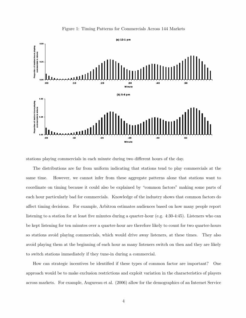
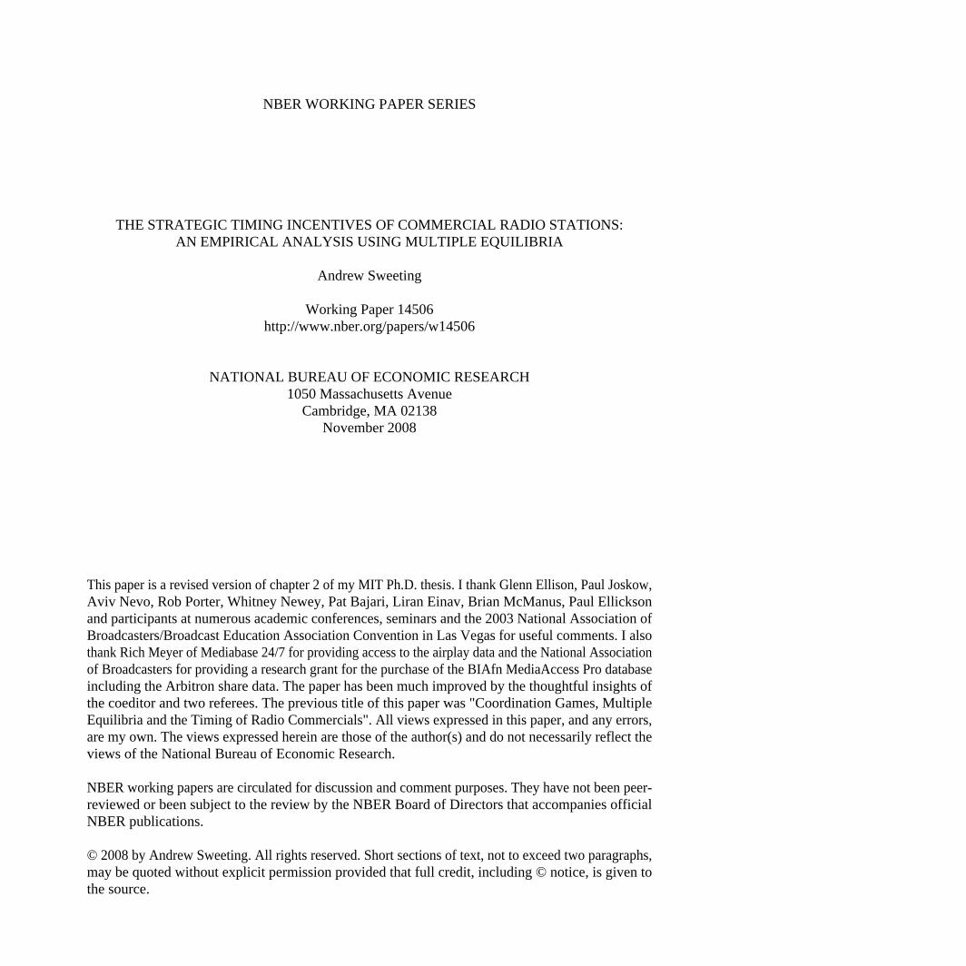
Figure 1: Timing Patterns for Commercials Across 144 Markets

(a) 12-1 pm

0.00

0.25

0.50

:00 :10 :20 :30 :40 :50M inute

Pro

po

rtio

n o

f sta

tio

n-h

ou

rs p

layi

ng

co

mm

erci

als

in m

inu

te

(b) 5-6 pm

0.00

0.25

0.50

:00 :10 :20 :30 :40 :50

Minute

Pro

po

rtio

n o

f st

atio

n-h

ou

rs p

layi

ng

com

mer

cial

s in

min

ute

(a) 12-1 pm

0.00

0.25

0.50

:00 :10 :20 :30 :40 :50M inute

Pro

po

rtio

n o

f sta

tio

n-h

ou

rs p

layi

ng

co

mm

erci

als

in m

inu

te

(b) 5-6 pm

0.00

0.25

0.50

:00 :10 :20 :30 :40 :50

Minute

Pro

po

rtio

n o

f st

atio

n-h

ou

rs p

layi

ng

com

mer

cial

s in

min

ute

stations playing commercials in each minute during two different hours of the day.

The distributions are far from uniform indicating that stations tend to play commercials at the

same time. However, we cannot infer from these aggregate patterns alone that stations want to

coordinate on timing because it could also be explained by “common factors” making some parts of

each hour particularly bad for commercials. Knowledge of the industry shows that common factors do

affect timing decisions. For example, Arbitron estimates audiences based on how many people report

listening to a station for at least five minutes during a quarter-hour (e.g. 4:30-4:45). Listeners who can

be kept listening for ten minutes over a quarter-hour are therefore likely to count for two quarter-hours

so stations avoid playing commercials, which would drive away listeners, at these times. They also

avoid playing them at the beginning of each hour as many listeners switch on then and they are likely

to switch stations immediately if they tune-in during a commercial.

How can strategic incentives be identified if these types of common factor are important? One

approach would be to make exclusion restrictions and exploit variation in the characteristics of players

across markets. For example, Augureau et al. (2006) allow for the demographics of an Internet Service

4

Provider’s (ISP) service area to affect its preferred modem technology. Service areas overlap creating

variation in the expected choices of an ISP’s competitors and this allows strategic incentives to be

identified. One might hope that exclusion restrictions could be found here as well. For example,

if timing preferences were to vary systematically across owners (some firms like Clear Channel own

stations in many markets) or across different music formats, then one might be able to identify strategic

incentives using plausibly exogenous variation in the ownership or format mix across markets.

Unfortunately I show that observable station characteristics have very little affect on timing choices,

especially during drivetime, so that even if the exclusion restrictions are valid, they will not be very

useful in identifying strategic incentives. Instead I emphasize a more novel approach to identification

which exploits the possible existence of multiple equilibria in the model and in the data. To see

the intuition suppose that stations play a timing game with two alternative timing choices (1 and 2)

which are equally attractive in terms of common factors (for example, neither is a quarter-hour). If

stations want to coordinate then there may be an equilibrium where stations cluster their commercials

at time 1 and another equilibrium where they cluster their commercials at time 2. If some markets

are in each equilibrium then the type of pattern that we would see in the data could look like Figure

2 which shows when stations in two markets played commercials during one particular hour. The

distributions in both markets have three peaks, just like the aggregate distribution, but they are at

noticeably different times. If stations want to play commercials at different times then we would expect

to observe excess dispersion within markets (market distributions less concentrated than the aggregate)

rather than clustering. If there is no strategic incentive then, if common factors are the same across

markets, then there is no reason why we should observe either excess clustering or dispersion relative

to the aggregate distribution. Therefore, if we can observe stations clustering at different times in

different markets and we can make some assumptions about how common factors vary across markets,

then we may be able to infer that stations want to coordinate on timing.

The idea that multiple equilibria can aid identification is not entirely new: in particular, Brock and

Durlauf (2001) make this argument in their analysis of non-linear peer effect models. The underlying

structure of our models is very similar, but I develop my results in the context of estimating a game

where the number of players is relatively small. In contrast, Brock and Durlauf consider settings with

5

Figure 2: Timing of Commercials in Orlando, FL and Rochester, NY on October 30, 2001 5-6 pm

(a ) O rla nd o, FL

0

1

2

3

4

5

:00 :05 :10 :15 :20 :25 :30 :35 :40 :45 :50 :55

M inute

Num

ber o

f sta

tions

pla

ying

co

mm

erci

als

in m

inut

e

(b ) Ro ch este r , NY

0

1

2

3

4

5

:00 :05 :10 :15 :20 :25 :30 :35 :40 :45 :50 :55M inute

Num

ber o

f sta

tions

pla

ying

co

mm

erci

als

in m

inut

e (a ) O rla nd o, FL

0

1

2

3

4

5

:00 :05 :10 :15 :20 :25 :30 :35 :40 :45 :50 :55

M inute

Num

ber o

f sta

tions

pla

ying

co

mm

erci

als

in m

inut

e

(b ) Ro ch este r , NY

0

1

2

3

4

5

:00 :05 :10 :15 :20 :25 :30 :35 :40 :45 :50 :55M inute

Num

ber o

f sta

tions

pla

ying

co

mm

erci

als

in m

inut

e

sufficiently many players that summary statistics on the actions of other players can simply be included

as regressors in a single agent analysis. My approach - which raises some additional identification

issues - is more naturally applicable in the type of settings usually considered by IO economists.

The obvious concern with relying on multiple equilibria for identification of strategic incentives

is that some forms of heterogeneity in common factors across markets could generate patterns which

look like multiple equilibria. I show that controlling for observable heterogeneity and allowing for

parametric forms of unobserved heterogeneity does not change my results. Perhaps more convincingly

I also show that there are differences in the results across markets and hours which are consistent with

coordination. For example, strategic incentives should be stronger when listeners are more likely to

switch stations (both θ parameters larger in the model). This is true during drivetime hours because

in-car listeners, who are more numerous during drivetime, are closer to their dials/preset buttons.4

4MacFarland (1997), p. 89, reports that, based on a 1994 survey, 70% of in-car listeners switch at least once duringa commercial break compared with 41% of at home and 29% of at work listeners. Arbitron estimates that 39.2% oflistening is in-car during drivetime compared with 27.4% 10 am-3 pm and 25.0% 7 pm-midnight (Fall 2001 data fromthe Listening Trends section of Arbitron’s website, www.arbitron.com). Abernethy (1991) estimates that in-car listenersswitch stations 29 times per hour on average.

6

Consistent with this, and with stations wanting to coordinate, I find greater clustering and estimate

a stronger incentive to coordinate during drivetime than outside drivetime. I also find that there is

greater coordination in smaller markets, which typically have fewer stations, which is consistent with

some models of listener behavior.

The paper is organized as follows. The rest of the introduction reviews the related literature.

Section 2 describes the data. Section 3 presents the model of the timing game. Sections 4 and 5

discuss identification and estimation. Section 6 presents the empirical results and Section 7 concludes.

1.1 Related Literature

The observation that radio and TV stations tend to play commercials at the same time has motivated

a small theoretical literature. Epstein (1998), Zhou (2000) and Kadlec (2001) assume that stations try

to maximize the audience of commercials and show that in equilibrium stations play commercials at

the same time. Sweeting (2006) provides theoretical models where strategic incentives should lead the

degree to which commercials overlap in equilibrium to vary with the propensity of listeners to switch

stations, which varies across hours, and market characteristics, such as the number of stations, own-

ership concentration and asymmetries in station listenership, together with some supporting reduced

form evidence. I provide further evidence for these differences in the current paper, which comes out

of the estimation of a more formal timing game.

I model stations as playing an incomplete information game. The incomplete information assump-

tion has typically been used for convenience when there are many players, many actions or strategies

are likely to be complicated (e.g., Seim (2006), Ellickson and Misra (2007), Augureau et al. (2006) and

the recent literature on dynamic games). In my setting stations make timing choices simultaneously

in real-time so incomplete information is more plausible. I present a simple test for imperfect infor-

mation and find that I cannot reject this assumption. Bajari et al. (2007b, hereafter BHNK) provide

formal identification results in incomplete information games, noting the current paper’s contribution

with respect to multiple equilibria. I use two common estimation procedures: a computationally light

two-step approach (e.g., BHNK) and the Nested Fixed Point algorithm (NFXP, Rust (1987)). The

two-step approach and the parameterization I use for the NFXP assume that a station uses the same

7

strategy throughout my data and I present three tests which support this assumption.

Multiple equilibria have received more attention in games of complete information. I borrow

from several papers in this literature (Bajari et al. (2007a), Bjorn and Vuong (1985), Ackerberg and

Gowrisankaran (2006), Tamer (2003)) when specifying an equilibrium selection mechanism to close the

model. Several recent papers, including Ciliberto and Tamer (2007) and Pakes et al. (2006), have

shown that it is possible to estimate at least bounds on parameters in complete information games

without specifying a selection mechanism. The emphasis in the current paper is different because I

actually use the existence of multiple equilibria to identify strategic incentives.

2 Data

The data on the timing of commercials are extracted from airplay logs collected by Mediabase 24/7, a

company which uses electronic technologies to collect data on music airplay.

2.1 Coverage of the Mediabase Sample

I use logs from the first five weekdays of each month in 2001 for 1,091 music stations, including

stations in the Adult Contemporary, Contemporary Hit Radio/Top 40, Country, Oldies, Rock and

Urban formats as defined by BIAfn’s MediaAccess Pro database.5 This database is also used to

allocate stations to 144 markets, including all of the largest radio markets in the US with the exception

of Puerto Rico.6 While some stations have listeners in multiple markets (e.g., Boston and Providence,

RI), most of a station’s listenership is in its market of license and I treat music stations licensed to a

market as players in the timing game.

Unfortunately, the Mediabase sample does not cover include every licensed music station. Table

1 summarizes the coverage of the sample, splitting markets into two groups based on market size.

In large markets, the sample includes over 70% of stations, and they account for over 86% of music

station listenership because Mediabase concentrates on larger stations. The sample contains a smaller

5 I combine stations in the Album Oriented Rock and Rock formats as stations in these formats play relatively similarmusic and seem to make similar timing choices. I drop observations for two station-quarters where BIAfn does notclassify the station into one of these six formats.

6 I drop observations from three markets (each with only one station) which enter the data only in December 2001.These stations were used in earlier versions of the paper without significant effects on the results.

8

Table 1: Coverage of the Airplay SampleLargest 70 Sample Markets Smallest 74 Sample MarketsNew York City, NY - Albuquerque, NM -

Knoxville, TN Muskegon, MI

Average number of 13.3 9.4music stations in market

Average number of sample 10.3 4.9stations in market

Average % of 86.6 66.5music listening accountedfor by sample stations

Note: statistics based on licensed commercial stations in the six formats listed above which had enoughlisteners to be rated by Arbitron throughout 2001

proportion of stations in smaller markets but it still includes two-thirds of music listenership. The

panel is unbalanced over time, both because Mediabase sample expands during the year and some

logs for individual station-days are missing. Overall there are 51,601 station-days of data, with up to

59 days per station. The issues which missing data create for estimating the model are discussed in

Section 5.

2.2 Airplay Logs

Table 2 shows an extract from an airplay log. The log lists the start time of each song and indicates

whether there was a commercial break between songs. I estimate whether any particular minute has

a commercial break using the following procedure:

1. the length of each song is estimated by the median time between songs with no commercials;7

2. a minute-by-minute schedule for each station-hour is created assuming that each song is played

its full length unless this would erase a commercial break or overlap the start of the next song;

and,

3. if the resulting breaks are more than five minutes long (a plausible maximum length), the break

is shortened to five minutes by sequentially taking minutes from the end and then the start of the7 If a song is played less than 10 times without being followed by a commercial break, I asssume that the song is four

minutes long, the median length of all songs.

9

Table 2: Extract from a Sample Airplay LogTime Artist Title Release Year5:02 PM LIFEHOUSE Hanging By A Moment 20005:06 PM 3 DOORS DOWN Kryptonite 20005:08 PM MORISSETTE, ALANIS You Oughta Know 19955:12 PM POLICE Roxanne 19795:18 PM PINK Get the Party Started 20015:22 PM BARENAKED LADIES The Old Apartment 19965:24 PM SUGAR RAY Little Saint Nick 19975:26 PM KEYS, ALICIA Fallin’ 20015:30 PM KRAVITZ, LENNY Dig In 2001Stop Set BREAK Commercials and/or Recorded Promotions -5:40 PM SHAGGY Angel 20005:44 PM TRAIN Something More 2001Stop Set BREAK Commercials and/or Recorded Promotions -5:54 PM GOO GOO DOLLS Black Balloon 19995:58 PM CREED With Arms Wide Open 2000

break. This procedure increases the possibility of measurement error, so I drop station-hours

with fewer than 8 songs as measurement errors are more likely when more time is unaccounted

for.

2.3 Definition of Timing Choices

In common with the existing literature I specify a discrete choice game to estimate stations’ strategic

incentives. To do this, I need to specify a small number of timing options which stations will choose

between. As the end of the hour has the most commercials, I classify stations into three groups: stations

which are playing commercials at 50 minutes past the hour, stations which are playing commercials

at 55 minutes past the hour and stations which are playing them at neither of these times. As I will

show in Section 5, I can make assumptions under which it is consistent to simplify the game in this

way. A complication arises if a station has commercials at both :50 and :55 (possible if the station

has a short song between two breaks) but as I will show in a moment only a few station-hours have

this feature and, for simplicity, I simply exclude them from the rest of the analysis.

While I have data from every hour of the day I focus the analysis on four hours. 4-5 pm and

5-6 pm are two hours in the middle of the afternoon drivetime period when many listeners will be in

their cars and any strategic incentives should be quite strong. I focus on the afternoon drive because

10

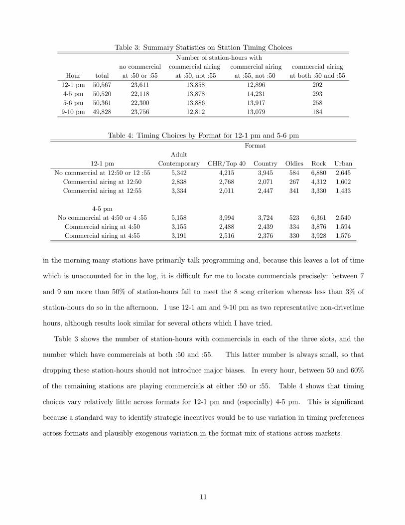
Table 3: Summary Statistics on Station Timing ChoicesNumber of station-hours with

no commercial commercial airing commercial airing commercial airingHour total at :50 or :55 at :50, not :55 at :55, not :50 at both :50 and :5512-1 pm 50,567 23,611 13,858 12,896 2024-5 pm 50,520 22,118 13,878 14,231 2935-6 pm 50,361 22,300 13,886 13,917 2589-10 pm 49,828 23,756 12,812 13,079 184

Table 4: Timing Choices by Format for 12-1 pm and 5-6 pmFormat

Adult12-1 pm Contemporary CHR/Top 40 Country Oldies Rock Urban

No commercial at 12:50 or 12 :55 5,342 4,215 3,945 584 6,880 2,645Commercial airing at 12:50 2,838 2,768 2,071 267 4,312 1,602Commercial airing at 12:55 3,334 2,011 2,447 341 3,330 1,433

4-5 pmNo commercial at 4:50 or 4 :55 5,158 3,994 3,724 523 6,361 2,540Commercial airing at 4:50 3,155 2,488 2,439 334 3,876 1,594Commercial airing at 4:55 3,191 2,516 2,376 330 3,928 1,576

in the morning many stations have primarily talk programming and, because this leaves a lot of time

which is unaccounted for in the log, it is difficult for me to locate commercials precisely: between 7

and 9 am more than 50% of station-hours fail to meet the 8 song criterion whereas less than 3% of

station-hours do so in the afternoon. I use 12-1 am and 9-10 pm as two representative non-drivetime

hours, although results look similar for several others which I have tried.

Table 3 shows the number of station-hours with commercials in each of the three slots, and the

number which have commercials at both :50 and :55. This latter number is always small, so that

dropping these station-hours should not introduce major biases. In every hour, between 50 and 60%

of the remaining stations are playing commercials at either :50 or :55. Table 4 shows that timing

choices vary relatively little across formats for 12-1 pm and (especially) 4-5 pm. This is significant

because a standard way to identify strategic incentives would be to use variation in timing preferences

across formats and plausibly exogenous variation in the format mix of stations across markets.

11

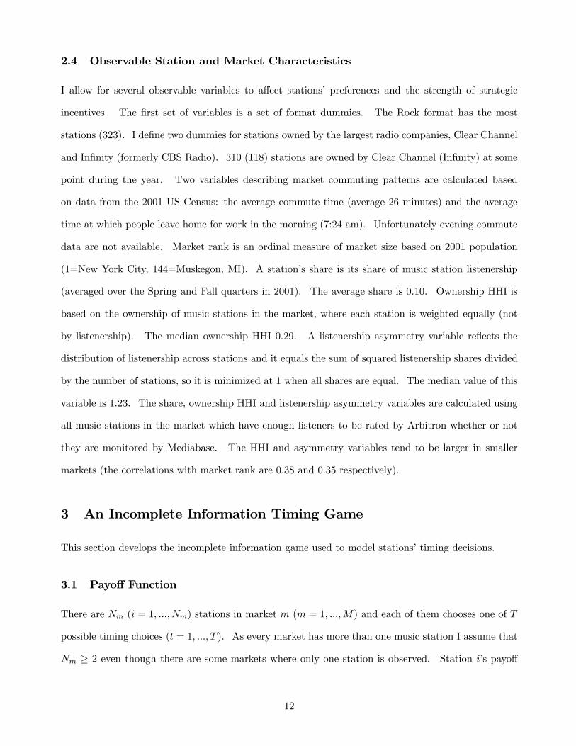
2.4 Observable Station and Market Characteristics

I allow for several observable variables to affect stations’ preferences and the strength of strategic

incentives. The first set of variables is a set of format dummies. The Rock format has the most

stations (323). I define two dummies for stations owned by the largest radio companies, Clear Channel

and Infinity (formerly CBS Radio). 310 (118) stations are owned by Clear Channel (Infinity) at some

point during the year. Two variables describing market commuting patterns are calculated based

on data from the 2001 US Census: the average commute time (average 26 minutes) and the average

time at which people leave home for work in the morning (7:24 am). Unfortunately evening commute

data are not available. Market rank is an ordinal measure of market size based on 2001 population

(1=New York City, 144=Muskegon, MI). A station’s share is its share of music station listenership

(averaged over the Spring and Fall quarters in 2001). The average share is 0.10. Ownership HHI is

based on the ownership of music stations in the market, where each station is weighted equally (not

by listenership). The median ownership HHI 0.29. A listenership asymmetry variable reflects the

distribution of listenership across stations and it equals the sum of squared listenership shares divided

by the number of stations, so it is minimized at 1 when all shares are equal. The median value of this

variable is 1.23. The share, ownership HHI and listenership asymmetry variables are calculated using

all music stations in the market which have enough listeners to be rated by Arbitron whether or not

they are monitored by Mediabase. The HHI and asymmetry variables tend to be larger in smaller

markets (the correlations with market rank are 0.38 and 0.35 respectively).

3 An Incomplete Information Timing Game

This section develops the incomplete information game used to model stations’ timing decisions.

3.1 Payoff Function

There are Nm (i = 1, ...,Nm) stations in market m (m = 1, ...,M) and each of them chooses one of T

possible timing choices (t = 1, ..., T ). As every market has more than one music station I assume that

Nm ≥ 2 even though there are some markets where only one station is observed. Station i’s payoff

12

from choosing action t is

πimt = Ximβt + αP−imt + εimt (1)

where P−imt is the proportion of other stations in the market choosing action t. This payoff function

is a “reduced form” in the sense that neither listener or advertiser behavior are modelled. A notable

assumption, given that I have panel data, is that the model is static rather than dynamic. Section 6

shows that I cannot reject that each station uses the same choice probabilities throughout the one-year

period of my data which is consistent with this static assumption (meaningful dynamics would cause

stations to change their choice probabilities in response to the actions of other stations).8

The first term (Ximβt) allows timing choices to have different average payoffs (e.g., lower for quarter-

hours) and for station characteristics to affect timing preferences. I make the standard normalization

that β1 = 0. Stations are identical when they do not differ in payoff-relevant characteristics.

The second term (αP−imt) determines the strategic interactions which are the focus of this paper.

If stations want to coordinate then α > 0 whereas if they want to differentiate then α < 0. I assume

that there are no strategic interactions across markets. The formulation embodies several assumptions,

such as α being the same across markets, which I will relax in Section 6.

The final term (εimt) is a random shock to a station’s payoff from making a particular timing

choice. I assume that εimt is private information to station i so that the game is one of incomplete

information. The interpretation of the εs in my setting is that on any particular day a station has

to fit commercial breaks around other pieces of programming (songs, competitions, weather updates)

in real time and, because it would annoy listeners to cut these types of programming off, this creates

some uncertainty about when commercials will be played.9 As this uncertainty is resolved in real

time in ways which should be hard for other stations to predict, the private information assumption is

reasonable. In Section 6 I will provide some evidence in favor of private information once I allow for

8One interpretation would be that any significant dynamics took place in years prior to my data and that there areno significant shocks during my data which would reintroduce dynamic forces.

9Modern scheduling software potentially gives program directors greater control over when commercials are played.However during drivetime stations typically use their most experienced DJs who are given a fair amount of discretion increating programming which appeals to the listener. It is notable that TV commercials placed precisely in pre-recordedprogramming tend to overlap more than radio commercials. Warren (2001), p. 24 describes how playing commercialsat a particular time “can be done some of the time. But it can’t be done consistently by very many stations. Few songsare 2:30 minutes long any more”. Gross (1988) says that the logistics involved in creating perfect “roadblocks” wouldbe “nightmare”.

13

a persistent component of non-strategic preferences which is observed by all stations but not by the

researcher.

3.2 Station Strategies and Bayesian Nash Equilibria

A station will choose the action which maximizes its expected payoffs given the strategies of other

stations, i.e., t will be chosen if and only if

Πimt(Ximt, σ−imt, (α, βt))−Πimt0(Ximt0 , σ−imt0 , (α, βt)) ≥ εimt0 − εimt ∀t0 6= t (2)

where Πimt(Ximt, σ−imt, (α, βt)) = Ximtβt + α

Pj 6=i σjmt

Nm − 1

and σjmt is the probability that station j chooses action t before the εs are realized and from the

perspective of other stations who do not observe the εjs. These choice probabilities are the most

convenient way to represent strategies. It is also useful to define Πim(α, β) as the vector of differences

between Πimt and Πim1 for actions t = 2, .., T

Πim(Xim, σ−imα, β) =

⎛⎜⎜⎜⎜⎜⎝Πim2(Xim2, σ−im2, (α, β2))−Πim1(σ−im1, α)

...

ΠimT (XimT , σ−imT , (α, βT ))−Πim1(σ−im1, α)

⎞⎟⎟⎟⎟⎟⎠ (3)

The best response function σim = Γ(Πim(Xim, σ−imα, β)) maps from Πim(Xim, σ−imα, β) into i’s

choice probabilities. The exact form of Γ depends on the distribution assumed for the εs. In a Bayesian

Nash equilibrium every station’s strategy is a best response, so that σ∗im = Γ(Πim(Xim, σ∗−im, β)) ∀i.

A Bayesian Nash equilibrium is symmetric if all stations with the same characteristics have the same

strategies. If α ≥ 0 then all equilibria must be symmetric.10 If α < 0 then there may be asymmetric

strategies but it is easy to show that, for given parameters, strategies tend towards being symmetric

as the number of stations increases.11

10Dropping market subscripts suppose that i and j are identical but that there are actions 1 and 2 for which σ∗i2 > σ∗j2and σ∗j1 > σ∗i1. This implies that k 6=i σ−k1 > k 6=j σ−k1 and that k 6=j σ−k2 > k 6=i σ−k2 so that Πj2 > Πi2 andΠi1 > Πj1. These inequalities, the fact that Xiβ1 = Xjβ1 and Xiβ2 = Xjβ2 for identical players and the property thatchoice probabilities must be increasing in Πit implies that σ∗i2 < σ∗j2 and σ∗j1 < σ∗i1, a contradiction.11The intuition is simple: as Nm increases j 6=i σ−imt

Nm−1 will look increasingly similar from the perspective of any twostations who will therefore have increasingly similar best response strategies.

14

Brouwer’s fixed point theorem guarantees the existence of at least one equilibrium but the number

of equilibria can vary with the parameters. As an illustration suppose that there are two stations (i

and j), two actions (1 and 2), that εs are distributed extreme value (logit) and that Xj2β2 = 0. Figure

3 shows their reaction functions for four different cases, where i(j)’s best response is on the vertical

(horizontal) axis. In all cases Xi2β2 = 0.1 so i has a preference for choosing action 2. In panel (a)

and (b) α > 0 so stations want to choose the same times for commercials and the reaction functions

slope upwards. In (a) the coordination incentive is relatively small and there is a single equilibrium.

It is larger in (b), so that the S shape of the reaction function (which comes from the shape of the

logit distribution) is more pronounced and there are 3 equilibria. The middle equilibrium (where

σ∗i2 = 0.441, σ∗j2 = 0.439) is unstable in the sense that the application of iterated best responses close

to this equilibrium would lead away from this equilibrium. The other equilibria involve the stations

choosing the same action with greater probability and the action which they are most likely to choose

differs across the equilibria. If i’s preference for action 2 was increased then its reaction function

would shift upwards and only the equilibrium involving coordination on action 2 would survive. This

is consistent with the common intuition (e.g., Augureau et al. (2006)) that multiple equilibria are

unlikely when stations differ substantially in payoff-relevant characteristics. I show that observable

characteristics have little impact on timing choices especially during drivetime hours. In panels (c)

and (d) α < 0 so stations want to choose different times for commercials. Once again when the

strategic incentives are strong there are three equilibria, but this time they involve stations tending to

choose different actions. A general property of the two action game when the εs have a bell-shaped

distribution (e.g., logit or normal) is that there are at most three equilibria.

3.3 Equilibrium Selection

Estimation can require closing the model with an “equilibrium selection mechanism”. This specifies

that with E possible equilibria, equilibrium e is played with probability λe,PE

e=1 λe = 1.

15

Figure 3: Reaction Functions and Multiple Equilibria

0 0.2 0.4 0.6 0.8 10

0.2

0.4

0.6

0.8

1(a) α=1

Station j`s probability for action 2

Sta

tion

i`s p

roba

bilit

y fo

r act

ion

2

i`s reaction function

j`s reaction function

(0.517,0.533)

0 0.2 0.4 0.6 0.8 10

0.2

0.4

0.6

0.8

1

Station j`s probability for action 2

Sta

tion

i`s p

roba

bilit

y fo

r act

ion

2

(b) α=2.4

(0.844,0.855)

(0.193,0.202)

(0.439,0.441)

0 0.2 0.4 0.6 0.8 10

0.2

0.4

0.6

0.8

1

Station j`s probability for action 2

Sta

tion

i`s p

roba

bilit

y fo

r act

ion

2

(c) α=-1

(0.483,0.533)

0 0.2 0.4 0.6 0.8 10

0.2

0.4

0.6

0.8

1

Station j`s probability for action 2

Sta

tion

i`s p

roba

bilit

y fo

r act

ion

2

(d) α=-2.4

(0.155,0.852)

(0.806,0.156)

(0.570,0.441)

16

4 Identification

The data consists of observable characteristics and, as outcomes, the timing choice of each station. The

parameters are identified if and only if a unique set of parameters gives rise to any set of probabilities

for each outcome. I separate the discussion into two parts: first, the assumptions under which the

payoff parameters are identified if the equilibrium choice probabilities of each station are known and

second, the conditions under which equilibrium choice probabilities can be identified from the data.

4.1 Identification of Payoff Parameters Given Equilibrium Choice Probabilities

Previous studies of identification in discrete choice incomplete information games (BHNK, Pesendorfer

and Schmidt-Dengler (2007)) have assumed that the researcher can observe equilibrium strategies for

each station (σ∗im). They have also assumed that a single equilibrium is played, and I will show

why multiple equilibria can provide additional identification in this case. Throughout I assume that

β1 = 0 and that the εs are iid with a known parametric distribution. BHNK, p. 9 argue that these

assumptions are necessary for identification. Hotz and Miller (1993) show that Γ function, which

maps differences in choice specific value functions to choice probabilities, can be inverted so that for

each distinct set of equilibrium choice probabilities there are T − 1 linearly independent equations ofthe form

Γ−1(σ∗im) = Ximtβt + α

µPj 6=i σjmt −

Pj 6=i σjm1

Nm − 1¶for t = 2, .., T (4)

4.1.1 Identical Stations

The helpful role of multiple equilibria can be seen most clearly when stations are identical (Xim is the

same for all stations in all markets). In this case there are T payoff parameters (β2, ..., βT , α). The

first identification result is negative.

Proposition 1. If stations are identical and a single symmetric equilibrium is played in every market

then the parameters are not identified.

Proof. If stations in all markets are identical and a single symmetric equilibrium is played then σ∗imt =

σ∗−imt = σ∗jnt ∀i, j,m, n, t so that the strategies of each station yield an identical set of linear equations.12

12The proportional formulation of the strategic incentive in the payoff function implies that symmetric equilibrium

17

There are T parameters and T − 1 linear equations so the parameters are not identified.The choice probabilities also place no restrictions or bounds on the parameters in this case, i.e., for

any α we can find βs which generate any observed set of equilibrium choice probabilities.13

Proposition 2. If stations are identical and at least two equilibria are played then the parameters are

identified.

Proof. One equilibrium provides T − 1 linear equations. A second equilibrium must have at least two

equilibrium choice probabilities which are different from the first, providing at least one additional

linearly independent equation. Hence, the T parameters are identified.

Additional equilibria would provide additional equations, so that the parameters will be overi-

dentified. The logic of the proof also shows that the parameters will be identified with asymmetric

equilibria, as there will be additional equations for each set of equilibrium choice probabilities.

4.1.2 Non-Identical Stations

If stations differ in observable characteristics which affect timing preferences then additional variation

can identify the parameters. In particular, suppose that exclusion restrictions can be made so that

a station’s own characteristics only directly affect its own timing preferences. In this case, variation

in the characteristics of other stations in a market will create additional sets of equations like (4)

as theP

j 6=i σjmts will vary for given values of Ximt.14 BHNK show that the parameters are non-

parametrically identified when there is sufficient variation in the characteristics of other stations. Of

course, multiple equilibria will still provide additional equations, and they may be particularly valuable

when variation in station characteristics is limited (e.g., there are a few discrete types). The helpful

role of multiple equilibria in this context is discussed by Brock and Durlauf (2001).

strategies will form equilibria in markets with any Nm ≥ 2.13Of course, if one observed markets with one station (so only non-strategic preferences would affect choices) then

one could identify strategic incentives from the differences in strategies between monopoly and oligopolistic markets.However, there are no monopoly markets in my data.14Note that having non-identical stations is not enough: variation in the set of station characteristics across markets

is also required. To see this suppose that there are three types of station and one station of each type in every market.If the same equilibrium is played in every market then there are 3(T − 1) + 1 parameters and 3(T − 1) equations so theparameters are not identified.

18

4.2 Identification of Equilibrium Choice Probabilities From Observed Outcomes

When a single symmetric equilibrium is played the identification of equilibrium choice probabilities

is trivial because, with infinite data, they can be estimated by the frequency with which each action

is chosen conditional on station characteristics. This argument fails with multiple or asymmetric

equilibria. However, the equilibrium choice probabilities are still identified under certain conditions.

4.2.1 Panel Data and Equilibrium Assumptions

Suppose that we observe a long panel of data on station choices. If we assume that each station uses

one strategy over time then we can identify each station’s equilibrium choice probabilities from its

own choice frequencies. This approach allows for asymmetric equilibria because the strategy of each

station can be identified without assuming that stations which appear identical use the same strategy.

The assumption that one equilibrium is played within each market over time has been made previously

by Pesendorfer and Schmidt-Dengler (2007) and Ellickson and Misra (2007). I will show below that

this assumption is consistent with the data.

4.2.2 Symmetric Equilibria and Identified Equilibrium Selection Mechanisms

With only cross-sectional data or a short panel it is necessary to identify the mixture of equilibrium

choice probabilities in the data. The equilibrium selection mechanism defines the frequency with which

each equilibrium occurs in the data.

The requirements for identification are easily seen when there are two actions (t = 1, 2), stations are

identical and equilibria are symmetric. Dropping market subscripts (markets are identical), suppose

that there are N stations and up to E equilibria and that in equilibrium e action 2 is chosen with

probability σ∗e2 and this equilibrium is played with probability λe. The probability that n2 stations

choose action 2, which can be observed in the data, is

Pr(N2 = n2) =EXe=1

λe

µN

n2

¶(σ∗e2)

n2(1− σ∗e2)N−n2 X

λe = 1 (5)

which is the pmf of a binomial mixture model with E possible components. This model has 2E − 1

19

parameters (E σ∗e2s and E − 1 λes) and there are N linearly independent equations (5). Teicher

(1963) shows that the parameters are identified if and only if there are N ≥ 2E − 1 stations (when N

varies across markets we need some markets with at least 2E− 1 stations). The same condition holdswith more actions (Kim (1984) and Elmore and Wang (2003)) which is intuitive because a multinomial

model can always be broken down into a set of binomial models with stations choosing an action or

its complement.

The intuition for identification of a mixture is that a mixture generates excess variance in the

number of stations choosing a particular outcome. Figure 4(a) shows a theoretical example. The

black bars show the pmf for the number of stations choosing action 2 when there are two choices,

N = 8, and there is a single symmetric equilibrium with identical stations and each station chooses

action 2 with probability 0.5. The white bars show the pmf when there is an equal mixture of two

symmetric equilibria. In the first equilibrium each station chooses action 2 with probability 0.6 and

in the second equilibrium each station chooses action 2 with probability 0.4. The probabilities of

outcomes with many stations choosing action 1 and outcomes with many stations choosing action 2

are both higher when there are multiple equilibria. Note that if stations want to choose different times

for commercials and an asymmetric equilibrium is played then outcomes with many stations choosing

the same action will have lower probability than could be generated by a single symmetric equilibrium.

In this case, there will be too little variance in the number of stations choosing a particular action, not

too much.

The remaining panels of Figure 4 show similar pictures constructed using data from 12-1 pm and 5-6

pm (as sample drivetime and non-drivetime hours). The red lines show the distribution of the observed

proportion of stations in a market-day-hour which play commercials at :55 out of the set of stations

playing commercials at either :50 or :55. I condition in this way in order to make the figure comparable

to (a), but stations making neither of these choices will not be ignored below. Panel (b) shows the

distribution for all markets, and panel (c) shows the distribution for the smallest 74 markets (roughly

breaking the dataset in half based on market size). For both size groups the density for 12-1 pm is

more concentrated around 0.5 than the density for 5-6 pm, consistent with there being more clustering

of commercials during drivetime. The solid black lines show the expected density if a single symmetric

20

Figure 4: Identification: Theory and Evidence

(ii) 5-6 pm

0

0.5

1

1.5

2

2.5

0 0.2 0.4 0.6 0.8 1

Proportion

Den

sity

(ii) 5-6 pm

0

0.5

1

1.5

2

2.5

0 0.2 0.4 0.6 0.8 1

Proportion

Den

sity

(a) Comparison of PDF for Number of Stations Choosing :55 for a Model with One or Two Equilibria

0

0.05

0.1

0.15

0.2

0.25

0.3

0 1 2 3 4 5 6 7 8

Number of Stations Choosing :55

pmf

Single Equilibrium, :55 Chosen with probability 0.5 Equal Mixture of Two Symmetric Equilibria, :55 Chosen with probabilities 0.6 and 0.4

(i) 12-1pm

0

0.5

1

1.5

2

2.5

0 0.2 0.4 0.6 0.8 1

Proportion

Den

sity

(i) 12-1 pm

0

0.5

1

1.5

2

2.5

0 0.2 0.4 0.6 0.8 1

Proportion

Den

sity

(b) Proportion of Stations Playing Commercials at :55 Conditional on Playing them at :50 or :55, All MarketsRed Line = Kernel Density for Actual Data, Black Lines = Expected Kernel Density for a Binomial Model +/- 1 Std Error

(c) Proportion of Stations Playing Commercials at :55 Conditional on Playing them at :50 or :55in 74 Smallest Markets (Albuquerque, NM and smaller)

21

equilibrium was played with each station choosing :55 with the probability that I observe it being chosen

in the actual data. Even though this simple model ignores any observable differences across stations

or markets which may affect timing choices, it fits the 12-1 pm data almost perfectly, with the actual

density being significantly different from the expected density (i.e., outside the +/- 1 standard error

dashed lines) at only a few points. On the other hand, for 5-6 pm the distribution has greater variance

than the single symmetric equilibrium model predicts. The differences are particularly large in smaller

markets, and this will be consistent with the results below where I find that incentives to coordinate

are stronger and multiple equilibria are more common in smaller markets during drivetime.15

The statistical mixture model literature has not considered models which would correspond to ones

in which stations in a market are not identical. However, the previous logic can be used to show that

identification does not become more difficult in this case. Suppose that there are two actions and S

observable types of station with Ns stations of type s using symmetric equilibrium choice probabilities

σ∗es. There are now S ∗E+E−1 parameters (S ∗E σ∗ess and E−1 λes) andSYs=1

(Ns+1)−1 observableprobabilities

Pr(N21 = n21, .., N2S = n2S) =EXe=1

λe

SYs=1

µNs

n2s

¶(σ∗es)

n1s(1− σ∗es)N−n1s X

λe = 1 (6)

Identification still depends on having enough stations relative to the number of equilibria but notice

that the number of observed probabilities (equations) increases geometrically in the number of types

while the number of parameters increases only linearly. This means that, for example, the equilibrium

choice probabilities and the selection mechanism are identified when one has two equilibria and three

stations each of a different type.

15Rysman and Greenstein (2005)’s Multinomial Test of Agglomeration and Dispersion (MTAD) provides an alternativeway of testing whether there are more markets where very many or very few stations choose the same action. Applyingthe MTAD for the binomial choice model (:50 or :55 conditional on one of these actions being chosen) shows that thereis significant clustering during both drivetime hours (p-values 0.000) but not outside drivetime (p-value 0.79 for 12-1pmand 0.44 for 9-10 pm ). Examining the multinomial choice (:50, :55 or neither) one finds significant clustering in all fourhours, although the test statistics are between 4 to 5 times larger for the drivetime hours.

22

5 Estimation

This section explains my estimation strategy. I start by showing why I am able to estimate stations’

strategic incentives using only a subset of choices, before outlining two different estimation procedures.

5.1 Estimation Using A Subset of Choices

It is computationally difficult to solve or estimate the game allowing for many possible timing choices,

multiple equilibria and different kinds of unobserved heterogeneity. However, I can still estimate

stations’ strategic incentives using data on just two choices (playing ads at :50 or :55) if the εs are iid

extreme value. To see why, label these timing choices 1 and 2 (β1 = 0). The probability that station

i chooses action 2 from the full set of T possible actions is

σ∗im2 =exp

³Ximβ2 + α j 6=i σ

∗jm2

Nm−1´

PTt=1 exp

³Ximβt + α j 6=i σ

∗jmt

Nm−1´ (7)

and the probability of action 2 conditional on action 1 or action 2 being chosen (σ∗im(2|1 or 2)) is

σ∗im(2|1 or 2) =exp

µXimβ2 + α

µj 6=i(2σ

∗jm(2|1 or 2)−1)σ∗jm(1 or 2)

N−1

¶¶1 + exp

µXimβ2 + α

µj 6=i(2σ

∗jm(2|1 or 2)−1)σ∗jm(1 or 2)

N−1

¶¶ (8)

where σ∗jm(1 or 2) is the probability that station j chooses action 1 or action 2. β2 and α can be

consistently estimated using the conditional choice probabilities in (8) as long as I adjust appropriately

for the probabilities that one of these choices is made by other stations (σ∗jm(1 or 2)).16

Variation in the proportion of stations choosing one of the two actions, potentially due to multiple

equilibria in the full game, can identify the parameters even if there is a single equilibrium in the

conditional two action game. The intuition is straightforward. Suppose that stations want to play

their commercials at the same time. If other stations are unlikely to play commercials at the end of

the hour then the incentives of a station which is playing a commercial then to try to coordinate with

16Note that it does not simplify matters to consider players choosing between action 2 and not action 2. In this case,the probability of choosing action 2 is given by (7) which depends on all of the parameters. One way of viewing theproblem is that, without additional parameters, it is not clear whether stations get a benefit from coordinating whenmany of them choose “not action 2”.

23

other stations are weak because it will likely only overlap with a small proportion of stations. On the

other hand, strategic incentives in the conditional game will be stronger when more stations are likely

to play commercials then.

This type of correlation is observed in the data. I created a dataset with observations on pairs of

stations in the same market, day and hour where both of the stations play commercials at either :50 or

:55. I also calculated the average proportion of other stations in the market which play commercials

at either of these times, and ran a linear probability model regressing a dummy variable for both of the

stations playing commercials at the same time (both at :50 or both at :55) on the proportion variable for

other stations. The correlation is positive in all hours, and it is significant at the 5% level for 4-5 pm.

When the proportion variable is interacted with the rank of the market (higher for smaller markets),

the interaction coefficients are positive and significant at the 0.1% level for both of the drivetime hours

(insignificant outside drivetime). These correlations are consistent with the results below which show

that stations want to coordinate on timing during drivetime and have stronger incentives in smaller

markets.

5.2 Two Step Estimation

The two step estimation approach follows the panel data identification argument set out above. If

a station uses the same strategy throughout my data then its equilibrium choice probabilities can be

estimated by

dσjmt =

PDjm

d=1 Ijdmt

Djm(9)

where Ijdmt is equal to 1 if station j chooses action t on day d and Djm is the number of days that

station j is observed in my data. These estimates can be used to calculate the terms in the inner

brackets on the right-hand side of (8) and a binomial logit model can be used to estimate β2 and α.

A necessary assumption is that whether an airplay log is missing is not related to a station’s timing

choice. Standard errors are calculated using a bootstrap where markets are resampled.

24

5.3 Nested Fixed Point Estimation (NFXP)

The NFXP algorithm solves for the conditional equilibrium choice probabilities at each iteration of the

parameters. The specification which I use assumes that each station uses one strategy throughout my

data. The probabilities that stations choose actions 1 or 2 are parameterized in the following flexible

way

σ∗im(1 or 2) =exp(β1 or 2 + ηi + ηm)

1 + exp(β1 or 2 + ηi + ηm)ηi ∼ N(0, γ2i ), ηm ∼ N(0, γ2m) (10)

which allows for persistent station and market heterogeneity. A market may have persistently few

commercials at :50 and :55 because stations coordinate on having commercials at a different time (e.g.,

:40). β1 or 2, γi and γm are parameters to be estimated together with β2 and α.17 ηi and ηm are

assumed to be known to all stations when they choose their conditional choice probabilities σ∗im(1 or 2).

The simplest NFXP model consists the equations (10) and (8), with no unobserved heterogeneity

in the β2 or α parameters. Estimation proceeds in the following steps:

1. S (50 or 100 depending on the model) sets of Halton draws for ei and em are drawn from a

standard normal distribution for each station and market. Draws are made and the game is

solved for all music stations whether or not they are in the Mediabase sample.18 ei and em are

held constant during estimation while ηsi = γiesi and ηsm = γme

sm vary with the parameters;

2. for each market for a given set of the parameters and draws,

(a) (10) is used to calculate σ∗im(1 or 2);

(b) the equilibrium choice probabilities σ∗im(2|1 or 2) are solved for by iterating best responses

(8). Experimentation showed that to reliably find multiple equilibria, it is necessary to

begin the iteration process from extreme points in the strategy space (e.g., every station

chooses action 1 with probability 0.99 or 0.01) and to update strategies rather slowly.19 I

take strategies to have converged when the choice probabilities change by less than 1e− 8.17Regressions (which are available on request) indicate that observable station and market characteristics have at most

small effects on the probability that actions 1 and 2 are chosen and for computational reasons these variables are notincluded in the specification.18 I include all commercial music stations with at least 1% shares of radio listening at some point during 2001.19For example, in some models I update choice probabilities by the maximum of 0.001 or 2.5% of the difference between

the current strategy and the best response. Updating more quickly can cause one of the equilibria to be missed.

25

This approach can only find stable and symmetric equilibria and, for given values of the

σ∗im(1 or 2)s, the conditional game can have at most two stable and symmetric equilibria;

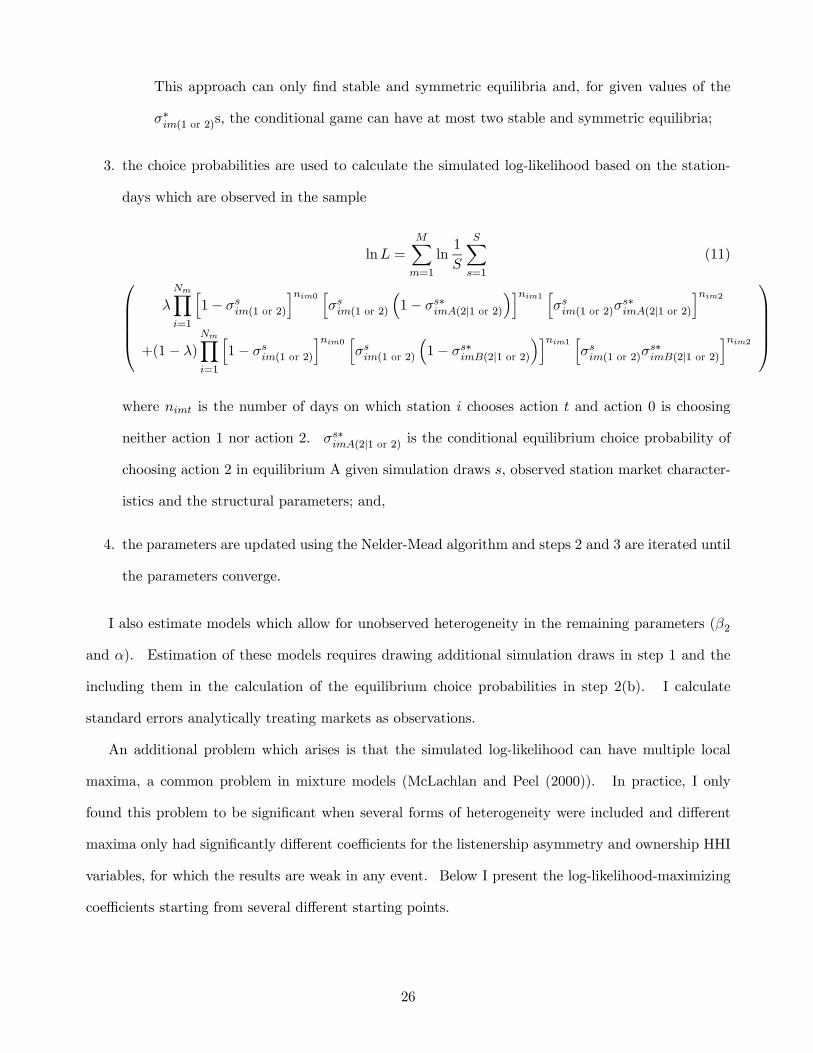
3. the choice probabilities are used to calculate the simulated log-likelihood based on the station-

days which are observed in the sample

lnL =MXm=1

ln1

S

SXs=1

(11)⎛⎜⎜⎜⎜⎝λNmYi=1

h1− σsim(1 or 2)

inim0 hσsim(1 or 2)

³1− σs∗imA(2|1 or 2)

´inim1 hσsim(1 or 2)σ

s∗imA(2|1 or 2)

inim2+(1− λ)

NmYi=1

h1− σsim(1 or 2)

inim0 hσsim(1 or 2)

³1− σs∗imB(2|1 or 2)

´inim1 hσsim(1 or 2)σ

s∗imB(2|1 or 2)

inim2⎞⎟⎟⎟⎟⎠

where nimt is the number of days on which station i chooses action t and action 0 is choosing

neither action 1 nor action 2. σs∗imA(2|1 or 2) is the conditional equilibrium choice probability of

choosing action 2 in equilibrium A given simulation draws s, observed station market character-

istics and the structural parameters; and,

4. the parameters are updated using the Nelder-Mead algorithm and steps 2 and 3 are iterated until

the parameters converge.

I also estimate models which allow for unobserved heterogeneity in the remaining parameters (β2

and α). Estimation of these models requires drawing additional simulation draws in step 1 and the

including them in the calculation of the equilibrium choice probabilities in step 2(b). I calculate

standard errors analytically treating markets as observations.

An additional problem which arises is that the simulated log-likelihood can have multiple local

maxima, a common problem in mixture models (McLachlan and Peel (2000)). In practice, I only

found this problem to be significant when several forms of heterogeneity were included and different

maxima only had significantly different coefficients for the listenership asymmetry and ownership HHI

variables, for which the results are weak in any event. Below I present the log-likelihood-maximizing

coefficients starting from several different starting points.

26

5.4 Comparison of the Two Estimation Procedures

I present the results using two estimation procedures because they have different strengths and weak-

nesses when applied to the type of data that I have. The two-step procedure would generate consistent

estimates if I had a sufficiently long panel of data without missing stations. In practice, there is limited

data on any station-hour (maximum 59 observations) and some stations are missing entirely, so that

my estimates of a station’s expectations about what other stations will choose (the inner brackets on

the right-hand side of (8)) are likely to be inaccurate. This is likely to bias the two-step estimates

of strategic incentives downwards and the bias may be larger in smaller markets where the sample is

less complete. However, the computational simplicity of the two-step procedure allows me to estimate

several specifications and to control for lots of observable characteristics. With these results I can

choose a plausible specification for the computationally-intensive NFXP procedure, which can gener-

ate consistent and efficient estimates as long as the fact that data is missing is not related to timing

choices. For this reason my discussion of the size of the strategic incentives will focus on the NFXP

results.

6 Empirical Results

I present the empirical results in the following order. Section 6.1 presents three tests of the assumption

that each station uses one strategy throughout my data. Sections 6.2 and 6.3 present the two-step

and NFXP estimates respectively.

Specifications are estimated separately for each hour, and I expect any strategic incentives to be

stronger during drivetime. I also allow strategic incentives to vary with three observable market

characteristics: market rank (higher for smaller markets), ownership concentration and listenership

asymmetry. The intuitions for why these variables may affect strategic incentives if stations want to

coordinate are fairly simple (Sweeting (2006) describes theoretical models examining these comparative

statics).

Smaller markets typically have fewer stations. If switching listeners try every station before

listening to a commercial then a station will only be able to maintain its audience during a commercial

27

if every station plays commercials at the same time. The probability that this happens increases when

there are fewer stations, increasing the incentive of every station to try to coordinate.20 A similar

result holds if listeners try only a sample of stations but they try more stations in larger markets.

Asymmetries in station listenership can strengthen coordination incentives if switchers are much more

likely to try one or two dominant stations. In this case, a station can keep most of its audience as long

as it plays commercials at the same time as just one or two stations giving it more incentive to try to

coordinate than in a market where stations are symmetric. Ownership concentration should lead to

more coordination because there are externalities in the timing game: a station’s timing decision will

affect the audience of other stations as well as its own. Commonly owned stations should internalize

these effects, and, because strategies are strategic complements if α > 0, common ownership should

lead to other stations coordinating more as well.21 If stations want to differentiate then we would

expect commercials to overlap less when ownership is more concentrated.

6.1 Testing for Changes in Station Strategies/Within Market Multiple Equilibria

The two-step procedure and the NFXP specification assume that each station uses the same strategy

throughout my data. This implies that the same equilibrium is played within a market over time. I

test this assumption using three tests which exploit different features of the data. One of tests (the

pairwise correlation test) also provides evidence in favor of the incomplete information assumption.

6.1.1 Modified Likelihood Ratio Test (MLRT)

MLRTs have been developed in the statistics literature (Chen et al. (2001) and Chen et al. (2004)) to

test for the appropriate number of components in binomial mixture models. Here I apply the Chen

et al. (2001) test market-by-market to examine whether there is evidence of multiple equilibria being

played within markets.

The test assumes that stations are identical. If a single equilibrium is played every day then the

probability that n2m stations are observed choosing action 2 on any given day is¡Nm

n2m

¢(σ∗2m)n2m(1 −

20 I present results from specifications which include market rank rather than the number of stations. Results usingthe latter variable are qualtitatively similar, but the coefficients vary more across specifications.21 I allow common ownership to affect coordination by allowing it to affect the strength of strategic incentives rather

than, for example, explicitly modelling joint decision making across multiple stations.

28

σ∗2m)Nm−n2m , the pmf for a binomial model with a single component. If two equilibria are played on

different days then the probability is (5) with E = 2, a binomial model with two components. Under

the alternative of two components the model is estimated using the modified log-likelihood

lM(λm, σ∗A2m, σ

∗B2m) = l(λm, σ

∗A2m, σ

∗B2m) + C log(4λm(1− λm)) (12)

where l(λm, σ∗A2m, σ∗B2m) is the standard log-likelihood for a two component mixture model and the

second term, where C is a positive constant, solves the problem that some of the parameters are

not identified under the null when only the standard log-likelihood is used. The test statistic is

M = lM(cλm, dσ∗A2m, dσ∗B2m)−lM(12 ,dσ∗2m,dσ∗2m)) where dσ∗2m is the choice probability for a single componentmixture, and its asymptotic distribution is an equal mixture of χ20 and χ21 distributions. Chen et al.

(2001) show that this test is the asymptotically most powerful under local alternatives.22

I apply the test defining the binomial actions in two different ways. The first way defines one

action as having a commercial at either :50 or :55 with the other action being having no commercial at

either of these times. The second way defines one action as having a commercial at :55 with the other

action not having a commercial at :55. The results are reported in part (a) of Table 5, which shows

the proportion of the markets where the null of a single component is rejected at the 5% level.23 The

proportion of markets where the null is rejected is small (less than 6%) in all station hours, consistent

with a single equilibrium being played within each market.24

6.1.2 Pairwise Station Correlation Test

The MLRT test is attractive in the sense that it uses the choices of all stations within a market

simultaneously, but it makes the unattractive assumption that stations within a market are identical.

The remaining tests do not make this assumption.

The correlation test examines whether there is any correlation in the timing choices of pairs of

22Chen et al. (2004) present a test where a two component model can be tested against a model with k > 2 components.This test is potentially useful for testing how many equilibria need to be allowed for.23The test only uses the 124 markets with at least three observed stations because, as discussed in Section 4, a two

component model is not identified with fewer than three stations.24One can also perform a joint test by adding the test statistics from each market and simulating this new statistic’s

asymptotic distribution. The null that there is only one equilibrium in each market cannot be rejected for any hour.The same conclusion holds for the joint version of the other tests.

29

Table 5: Test Results for Within Market Multiple EquilibriaAction 1: Commercial at :50 or :55 Commercial at :55Action 0: No Commercial at :50 or :55 No Commercial at :55

(a) Modified Likelihood Ratio Test: Proportion ofMarkets with Test Statistic Significant at 5% Level (One Sided)

12-1 pm 0.035 0.0564-5 pm 0.042 0.0145-6 pm 0.028 0.0079-10 pm 0.035 0.042

(b) Station Pairwise Correlation Test: Proportionof Pairs With Significant Correlations at 5% Level (Two Sided)

12-1 pm 0.058 0.0504-5 pm 0.047 0.0425- 6 pm 0.051 0.0509-10 pm 0.053 0.049

(c) Station Runs Test: Proportion ofStations With Significant Runs at 5% Level (Two Sided)

12-1 pm 0.062 0.0604-5 pm 0.062 0.0505-6 pm 0.064 0.0509-10 pm 0.048 0.044

stations in the same market. If a market switches from one equilibrium to another then stations’

strategies should change at the same time causing changes in their actions to be correlated. On the

other hand, if each station uses the same strategy every day (the null hypothesis) then actions will

only vary due to the iid ε payoff shocks so that actions should display no time-series correlation.

The correlation test also tests the incomplete information assumption, allowing for there to be a

fixed component of station preferences which does not vary from day-to-day and which is known to all

stations (this will be allowed for in some of the specifications below). Under incomplete information

a station’s strategy is a mapping from its own εs to its timing choices. On the other hand, under

complete information a station’s strategy will be a mapping from all stations’ εs to its timing choices

so that, even if the εs are iid and strategies do not change, there should be correlations in their choices.

I implement the test using the choice definitions assumed for the MLRT test. For each pair of

stations in the same market I calculate the correlation coefficient for these binary actions.25 The results

25The significance of the estimated correlation coefficient ρ is assessed using a t-distribution with (n − 2) degrees offreedom where n is the number of days when both stations in the pair are observed in the data.

30

are reported in part (b) of Table 5. There are only significant correlations for a small proportion of

pairs (and in these cases there is a roughly equal mix of positive and negative correlations) consistent

with incomplete information and with stations using the same strategies over time.

6.1.3 Runs Test26

The final test is a “runs test” which looks for serial correlation in a station’s own choices. A change

in a station’s strategy during the year should affect how frequently it makes a particular timing choice

on consecutive days. The test is implemented by defining binary choices as before, ordering the data

for each station by the calendar date and calculating how many runs there are of a particular choice

and whether there are more or less runs than one would expect if the data was randomly ordered.27

The results are reported in part (c) of Table 5. Once again, the test statistic is only significant for a

small proportion of stations.

6.2 Two Step Estimates

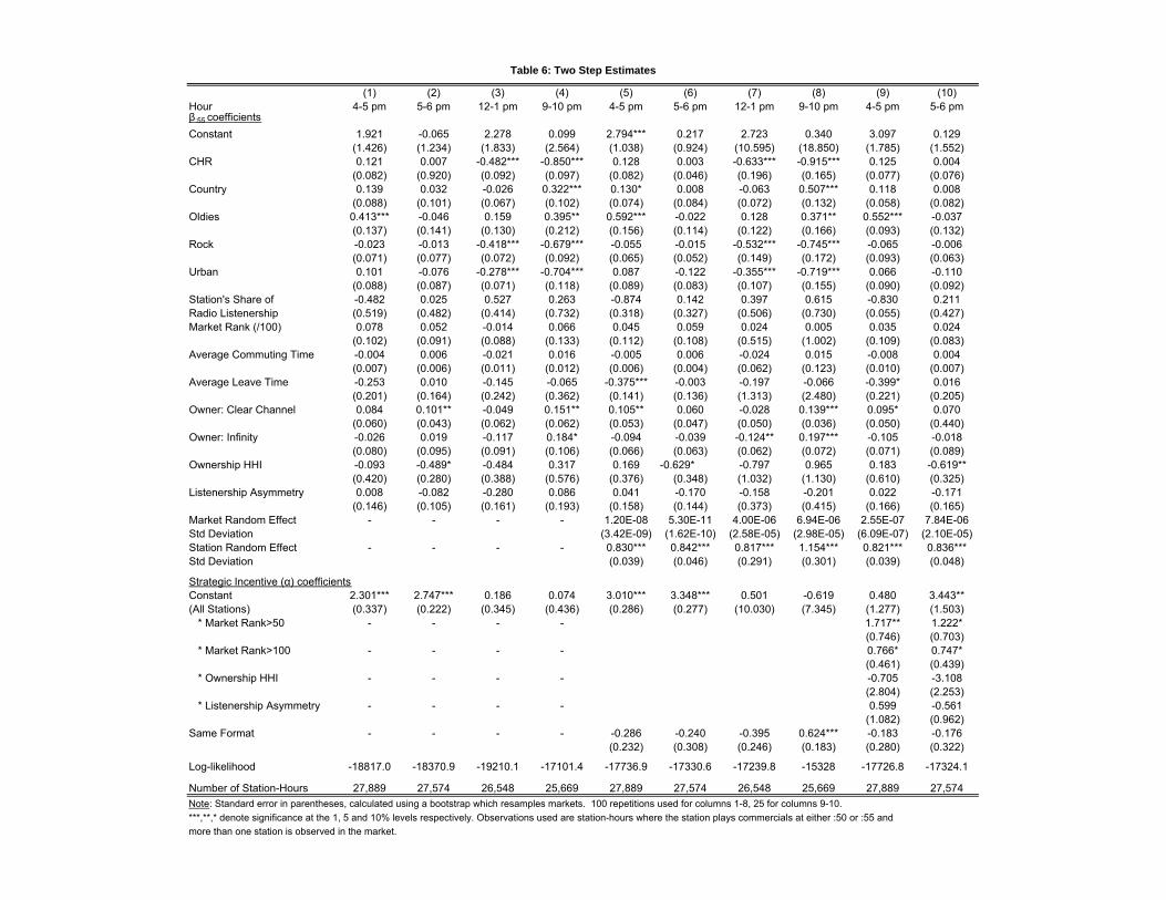
Table 6 presents the two step results. Columns (1)-(4) present estimates for each hour for specifications

which allow for observable heterogeneity in non-strategic preferences (β:55) but assume that strategic

incentives (α) are identical across markets and symmetric across stations within a market. The

estimated α is positive and significant at the 1% level for both drivetime hours, implying that stations

do want to play commercials at the same time. Very few of the covariates affecting non-strategic

preferences are statistically significant (Oldies at the 1% level for 4-5 pm and Clear Channel and

ownership HHI at 5% and 10% levels for 5-6 pm). These coefficients are also small: for example,

the Clear Channel coefficient for 5-6 pm implies that the conditional probability that a station has

a commercial at :55 increases by 0.025 when the station is owned by Clear Channel compared with

a mean probability of 0.50. The lack of significant shifters of non-strategic preferences implies that

“exclusion restriction” approaches to identification are likely to be ineffective.

26 I woukd like to thank one of my referees for suggesting this test.27For a (0,1) action, a run is defined as a sequence of identical choices (e.g., 000 or 11). When n0s is the number

of 0s chosen, the expected number of runs is 2n0sn1sn0s+n1s

+ 1 and the normal approximation to the test statistic is zs =rs− 2n0sn1s

n0s+n1s+1

2n0sn1s(2n0sn1s−(n0s+n1s)(n0s+n1s)

2(n0s+n1s−1)where rs is the number of runs.

31

(1) (2) (3) (4) (5) (6) (7) (8) (9) (10)Hour 4-5 pm 5-6 pm 12-1 pm 9-10 pm 4-5 pm 5-6 pm 12-1 pm 9-10 pm 4-5 pm 5-6 pmβ:55 coefficientsConstant 1.921 -0.065 2.278 0.099 2.794*** 0.217 2.723 0.340 3.097 0.129

(1.426) (1.234) (1.833) (2.564) (1.038) (0.924) (10.595) (18.850) (1.785) (1.552)CHR 0.121 0.007 -0.482*** -0.850*** 0.128 0.003 -0.633*** -0.915*** 0.125 0.004

(0.082) (0.920) (0.092) (0.097) (0.082) (0.046) (0.196) (0.165) (0.077) (0.076)Country 0.139 0.032 -0.026 0.322*** 0.130* 0.008 -0.063 0.507*** 0.118 0.008

(0.088) (0.101) (0.067) (0.102) (0.074) (0.084) (0.072) (0.132) (0.058) (0.082)Oldies 0.413*** -0.046 0.159 0.395** 0.592*** -0.022 0.128 0.371** 0.552*** -0.037

(0.137) (0.141) (0.130) (0.212) (0.156) (0.114) (0.122) (0.166) (0.093) (0.132)Rock -0.023 -0.013 -0.418*** -0.679*** -0.055 -0.015 -0.532*** -0.745*** -0.065 -0.006

(0.071) (0.077) (0.072) (0.092) (0.065) (0.052) (0.149) (0.172) (0.093) (0.063)Urban 0.101 -0.076 -0.278*** -0.704*** 0.087 -0.122 -0.355*** -0.719*** 0.066 -0.110

(0.088) (0.087) (0.071) (0.118) (0.089) (0.083) (0.107) (0.155) (0.090) (0.092)Station's Share of -0.482 0.025 0.527 0.263 -0.874 0.142 0.397 0.615 -0.830 0.211Radio Listenership (0.519) (0.482) (0.414) (0.732) (0.318) (0.327) (0.506) (0.730) (0.055) (0.427)Market Rank (/100) 0.078 0.052 -0.014 0.066 0.045 0.059 0.024 0.005 0.035 0.024

(0.102) (0.091) (0.088) (0.133) (0.112) (0.108) (0.515) (1.002) (0.109) (0.083)Average Commuting Time -0.004 0.006 -0.021 0.016 -0.005 0.006 -0.024 0.015 -0.008 0.004

(0.007) (0.006) (0.011) (0.012) (0.006) (0.004) (0.062) (0.123) (0.010) (0.007)Average Leave Time -0.253 0.010 -0.145 -0.065 -0.375*** -0.003 -0.197 -0.066 -0.399* 0.016

(0.201) (0.164) (0.242) (0.362) (0.141) (0.136) (1.313) (2.480) (0.221) (0.205)Owner: Clear Channel 0.084 0.101** -0.049 0.151** 0.105** 0.060 -0.028 0.139*** 0.095* 0.070

(0.060) (0.043) (0.062) (0.062) (0.053) (0.047) (0.050) (0.036) (0.050) (0.440)Owner: Infinity -0.026 0.019 -0.117 0.184* -0.094 -0.039 -0.124** 0.197*** -0.105 -0.018

(0.080) (0.095) (0.091) (0.106) (0.066) (0.063) (0.062) (0.072) (0.071) (0.089)Ownership HHI -0.093 -0.489* -0.484 0.317 0.169 -0.629* -0.797 0.965 0.183 -0.619**

(0.420) (0.280) (0.388) (0.576) (0.376) (0.348) (1.032) (1.130) (0.610) (0.325)Listenership Asymmetry 0.008 -0.082 -0.280 0.086 0.041 -0.170 -0.158 -0.201 0.022 -0.171

(0.146) (0.105) (0.161) (0.193) (0.158) (0.144) (0.373) (0.415) (0.166) (0.165)Market Random Effect - - - - 1.20E-08 5.30E-11 4.00E-06 6.94E-06 2.55E-07 7.84E-06Std Deviation (3.42E-09) (1.62E-10) (2.58E-05) (2.98E-05) (6.09E-07) (2.10E-05)Station Random Effect - - - - 0.830*** 0.842*** 0.817*** 1.154*** 0.821*** 0.836***Std Deviation (0.039) (0.046) (0.291) (0.301) (0.039) (0.048)

Strategic Incentive (α) coefficientsConstant 2.301*** 2.747*** 0.186 0.074 3.010*** 3.348*** 0.501 -0.619 0.480 3.443**(All Stations) (0.337) (0.222) (0.345) (0.436) (0.286) (0.277) (10.030) (7.345) (1.277) (1.503) * Market Rank>50 - - - - 1.717** 1.222*

(0.746) (0.703) * Market Rank>100 - - - - 0.766* 0.747*

(0.461) (0.439) * Ownership HHI - - - - -0.705 -3.108

(2.804) (2.253) * Listenership Asymmetry - - - - 0.599 -0.561

(1.082) (0.962)Same Format - - - - -0.286 -0.240 -0.395 0.624*** -0.183 -0.176

(0.232) (0.308) (0.246) (0.183) (0.280) (0.322)

Log-likelihood -18817.0 -18370.9 -19210.1 -17101.4 -17736.9 -17330.6 -17239.8 -15328 -17726.8 -17324.1

Number of Station-Hours 27,889 27,574 26,548 25,669 27,889 27,574 26,548 25,669 27,889 27,574Note: Standard error in parentheses, calculated using a bootstrap which resamples markets. 100 repetitions used for columns 1-8, 25 for columns 9-10.***,**,* denote significance at the 1, 5 and 10% levels respectively. Observations used are station-hours where the station plays commercials at either :50 or :55 and more than one station is observed in the market.

Table 6: Two Step Estimates

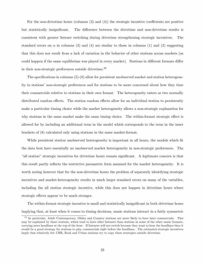
For the non-drivetime hours (columns (3) and (4)) the strategic incentive coefficients are positive

but statistically insignificant. The difference between the drivetime and non-drivetime results is

consistent with greater listener switching during drivetime strengthening strategic incentives. The

standard errors on α in columns (3) and (4) are similar to those in columns (1) and (2) suggesting

that this does not result from a lack of variation in the behavior of other stations across markets (as

could happen if the same equilibrium was played in every market). Stations in different formats differ

in their non-strategic preferences outside drivetime.28

The specifications in columns (5)-(8) allow for persistent unobserved market and station heterogene-

ity in stations’ non-strategic preferences and for stations to be more concerned about how they time

their commercials relative to stations in their own format. The heterogeneity enters as two normally

distributed random effects. The station random effects allow for an individual station to persistently

make a particular timing choice while the market heterogeneity allows a non-strategic explanation for

why stations in the same market make the same timing choice. The within-format strategic effect is

allowed for by including an additional term in the model which corresponds to the term in the inner

brackets of (8) calculated only using stations in the same market-format.

While persistent station unobserved heterogeneity is important in all hours, the models which fit

the data best have essentially no unobserved market heterogeneity in non-strategic preferences. The

“all station” strategic incentives for drivetime hours remain significant. A legitimate concern is that

this result partly reflects the restrictive parametric form assumed for the market heterogeneity. It is

worth noting however that for the non-drivetime hours the problem of separately identifying strategic

incentives and market-heterogeneity results in much larger standard errors on many of the variables,

including the all station strategic incentive, while this does not happen in drivetime hours where

strategic effects appear to be much stronger.

The within-format strategic incentive is small and statistically insignificant in both drivetime hours

implying that, at least when it comes to timing decisions, music stations interact in a fairly symmetric

28 In particular, Adult Contemporary, Oldies and Country stations are more likely to have later commercials. Thismay be explained by these stations, which tend to have older listeners than stations in some of the other music formats,carrying news headlines at the top of the hour. If listeners will not switch because they want to hear the headlines then itwould be a good strategy for stations to play commercials right before the headlines. The estimated strategic incentivesimply that relatively few CHR, Rock and Urban stations try to copy these strategies outside drivetime.

33

way. This finding is plausible if listeners switch primarily between preset stations and tend to preset

one station in each format.29 The format strategic incentive for 9-10 pm is significant but it only

offsets the negative and insignificant all station coefficient.

Columns (9) and (10) allow the all station strategic incentive to vary with observable market

characteristics (market rank, ownership concentration and listenership asymmetry) during drivetime.

The positive market rank coefficients are consistent with there being more coordination in smaller

markets but they are only weakly significant. The NFXP results will support the suggestion that

this may be due to the incomplete sample biasing the estimates of α in smaller markets. None of the

ownership or listenership asymmetry interaction coefficients are significant.

I have also estimated several specifications whose results are not reported. One of these allows

for a non-linear strategic incentive by including the square of the variable which multiples the α

coefficient in (8). Nonlinearities might arise if a station has an incentive to play its commercials

at a different time, to attract a large number of switchers, once the vast majority of other stations

are coordinating. The coefficients on the squared term in specification like columns (1)-(4) are all

statistically insignificant (e.g. 0.417 (1.234) for 4-5 pm and -0.586 (0.844) for 5-6 pm) with the other

coefficients almost unchanged. This result could be explained by linearity being the correct model or

by the variation in other stations’ strategies being too limited to identify more complicated effects.

6.3 NFXP Estimates and the Strength of Coordination Incentives

The simplest NFXP specification, whose results are reported in columns (1)-(4) of Table 7, assumes

that there is no unobserved heterogeneity in either β:55 or α. I allow at most one observable station-

specific variable to affect non-strategic preferences. Based on the two-step results, this variable is an

Oldies dummy for 4-5 pm and a dummy for CHR, Rock and Urban stations outside drivetime.30

The estimates of α are positive and significant for both of the drivetime hours, implying that

29 For example, I have News, Sports, Adult Contemporary, Country and Rock stations preset and if I want to skip acommercial then I would usually switch between these stations. Of course, several AC may have competed directly onprogramming (but not timing) to be my AC preset choice. Arbitron data supports the suggestion that stations sharelisteners as much across formats as within formats. For example, in Fall 2002 there were 6 Rock and 9 non-Rock homecontemporary music stations in Boston. On average 15.6% of the listeners to a Rock station listened to each of theother Rock stations and 15.3% of the listeners to a Rock station listened to each of the non-Rock stations (“the cumeduplication” tables in Arbitron (2003)).30A few stations change formats during 2001. When estimating the model I treat stations as being in their Spring

2001 formats throughout the year.

34

Hour 4-5 pm 5-6 pm 12-1 pm 9-10 pm 4-5 pm 5-6 pm 12-1 pm 9-10 pm 4-5 pm 5-6 pm

β:55 coefficientsConstant 0.001 0.002*** 0.199*** 0.560*** 0.001 0.001 0.216*** 0.532*** 0.001 0.004

(0.001) (0.000) (0.009) (0.008) (0.004) (0.001) (0.011) (0.008) (0.009) (0.004)Format Variable 0.005 N/A -0.417*** -0.932*** 0.005 N/A -0.474*** -0.938*** 0.005 N/A(see notes for definition) (0.008) (0.015) (0.010) (0.033) (0.015) (0.011) (0.016)Station Random Effect, Std Deviation 0.451*** 0.412***

- - - - - - - - (0.009) (0.009)

Strategic Incentives (α)Constant 3.304*** 3.404*** 1.818*** 0.476*** 0.106 0.200 0.125 0.025 0.107 0.706***

(0.006) (0.006) (0.104) (0.123) (0.261) (0.325) (0.308) (0.359) (0.118) (0.176)Market Rank (Linear Effect) - - - - 0.021 0.010 0.024 0.003 0.021 0.035

(0.139) (0.171) (0.860) (0.631) (0.338) (0.277)Market Rank ≥ 50 - - - - 1.205*** 1.741*** 0.119 0.020 1.214*** 1.790***

(0.119) (0.322) (0.444) (0.227) (0.236) (0.187)Market Rank ≥ 100 - - - - 1.563*** 1.177*** 0.252 0.011 1.574*** 0.855***

(0.171) (0.102) (0.437) (0.332) (0.194) (0.160)Listenership Asymmetry - - - - 0.099*** 0.101*** 0.076 0.008 0.100 -0.203***(normalized mean 0, std deviation 1) (0.021) (0.020) (0.175) (0.118) (0.069) (0.044)Ownership HHI - - - - 0.052 0.053 0.053 0.011 0.052 -0.055(normalized mean 0, std deviation 1) (0.050) (0.024) (0.150) (0.149) (0.074) (0.047)Market Random Effect, Std. Deviation - - - - 2.359*** 1.183*** 1.838*** 2.450*** 2.165*** 0.878***

(0.201) (0.050) (0.168) (0.168) (0.090) (0.051)Probability that :50 or :55 are chosenβ1 or 2 0.302*** 0.312*** 0.139*** 0.047*** 0.306*** 0.294*** 0.217*** 0.200*** 0.309*** 0.269***

(0.009) (0.005) (0.009) (0.010) (0.018) (0.009) (0.011) (0.013) (0.006) (0.007)Station Random Effect, Std Deviation 0.197*** 0.457*** 0.257*** 0.260*** 0.002 0.341*** 0.254*** 0.237*** 0.002 0.025**

(0.012) (0.006) (0.013) (0.013) (0.023) (0.007) (0.012) (0.011) (0.010) (0.009)Market Random Effect, Std Deviation 0.397*** 0.707*** 0.250*** 0.319*** 0.344*** 0.647*** 0.294*** 0.371*** 0.349*** 0.402***

(0.014) (0.009) (0.009) (0.011) (0.014) (0.014) (0.011) (0.016) (0.007) (0.008)Equilibrium Selectionλ 0.475*** 0.524*** NI NI 0.520*** 0.400*** 0.632 0.511 0.524*** 0.498**(NI= not identified when parameters do not (0.018) (0.068) (0.088) (0.084) (0.596) (0.369) (0.135) (0.220)support multiple equilibria for any simulationdraws)

Log-likelihood -52,857.60 -52,546.20 -52,712.70 -51,166.70 -52,587.30 -52,307.10 -52,698.50 -51,101.40 -52,326.40 -51,804.00

Number of Station-Hours 50,227 50,103 50,365 49,644 50,227 50,103 50,365 49,644 50,227 50,103Notes: Standard errors in parantheses. ***,**,* denote statistic significance at the 1, 5 and 10% levels respectively. Estimation by simulated maximum likelihood using a Nelder-Mead search algorithm.Number of simulations per station/market=100 for Model 1 and =50 for Models 2 and 3. Format variable: for 4-5 pm an Oldies dummy, for 12-1 pm and 9-10 pm a dummy for CHR, Rock and Urban stations.

Model 1 Model 2 Model 3

Table 7: NFXP Estimates

Station and Market Heterogeneity in Probabilities of Adds Market Heterogeneity in Strategic Incentives Adds Station Heterogeneityin Preferences for :55Choosing :50 or :55

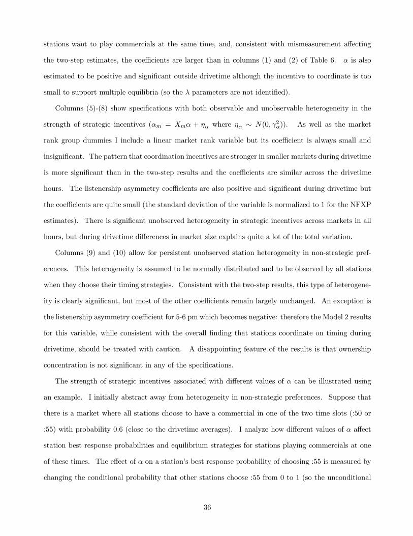
stations want to play commercials at the same time, and, consistent with mismeasurement affecting

the two-step estimates, the coefficients are larger than in columns (1) and (2) of Table 6. α is also

estimated to be positive and significant outside drivetime although the incentive to coordinate is too

small to support multiple equilibria (so the λ parameters are not identified).

Columns (5)-(8) show specifications with both observable and unobservable heterogeneity in the

strength of strategic incentives (αm = Xmα + ηα where ηα ∼ N(0, γ2α)). As well as the market

rank group dummies I include a linear market rank variable but its coefficient is always small and

insignificant. The pattern that coordination incentives are stronger in smaller markets during drivetime

is more significant than in the two-step results and the coefficients are similar across the drivetime

hours. The listenership asymmetry coefficients are also positive and significant during drivetime but

the coefficients are quite small (the standard deviation of the variable is normalized to 1 for the NFXP

estimates). There is significant unobserved heterogeneity in strategic incentives across markets in all

hours, but during drivetime differences in market size explains quite a lot of the total variation.

Columns (9) and (10) allow for persistent unobserved station heterogeneity in non-strategic pref-

erences. This heterogeneity is assumed to be normally distributed and to be observed by all stations

when they choose their timing strategies. Consistent with the two-step results, this type of heterogene-

ity is clearly significant, but most of the other coefficients remain largely unchanged. An exception is

the listenership asymmetry coefficient for 5-6 pm which becomes negative: therefore the Model 2 results

for this variable, while consistent with the overall finding that stations coordinate on timing during

drivetime, should be treated with caution. A disappointing feature of the results is that ownership

concentration is not significant in any of the specifications.

The strength of strategic incentives associated with different values of α can be illustrated using

an example. I initially abstract away from heterogeneity in non-strategic preferences. Suppose that

there is a market where all stations choose to have a commercial in one of the two time slots (:50 or

:55) with probability 0.6 (close to the drivetime averages). I analyze how different values of α affect

station best response probabilities and equilibrium strategies for stations playing commercials at one

of these times. The effect of α on a station’s best response probability of choosing :55 is measured by

changing the conditional probability that other stations choose :55 from 0 to 1 (so the unconditional

36

probability that they choose :55 changes from 0 to 0.6). The second column of Table 8 reports the

change in the best response. The third column reports the associated stable Bayesian Nash equilibrium

strategies. An entry of “(0.6,0.4)” means that there is one equilibrium where stations choose :55 with

conditional probability 0.6 and :50 with conditional probability 0.4 and another equilibrium where

these probabilities are reversed. To interpret the table, recall that the estimated drivetime value of α

for 4-5 pm for NFXP Model 1 is 3.3 and that the mean values of α for the three market size groups

for NFXP Model 2 are 0.04 (markets ranked 1-49), 1.34 (50-99) and 2.9 (above 100) with standard

deviation 2.36. The values of α are very similar for Model 3 and they are broadly similar for 5-6 pm.

Even for quite low values of α, a station’s best response is quite sensitive to the strategies of other

stations: for example, when α = 1 changes in the strategies of other stations can change a station’s

optimal conditional choice probability by almost 0.3. However, α = 1 results in no equilibrium

coordination in the sense that each station chooses each time with equal probability. The logic for

this result is quite simple (and can be seen graphically by centering the reaction functions in Figure

3(a)): if one station increased its probability of choosing :55, the best response of other stations would

be to increase their probabilities but by less, and the iteration of best responses would return stations

to making each choice with equal probability. Therefore observing that commercials do not overlap

that much does not imply that a station would not have quite strong incentives to coordinate if other

stations played them at the same time. As α increases above 3, multiple equilibria can be supported

and the stable equilibria involve greater overlap of commercials. For example, if α = 3.5 (a plausible

value in smaller markets during drivetime) an equilibrium can be supported where stations choose :55

with probability 0.685, so that the probability that two stations play commercials at the same time is

14% higher than if they choose each time with equal probability.

As already mentioned, there are externalities in the timing game which reduce equilibrium coordi-

nation. The last column of Table 8 quantifies the equilibrium effects of these externalities by showing

the strategies which would maximize stations’ expected joint payoffs. The calculation, which follows

one presented by Brock and Durlauf (2001), assumes that the εs remain private information. For low

levels of α, joint payoff-maximizing strategies still involve no coordination. However, as α increases

strategies rapidly shift to involving much more coordination than equilibrium strategies, with almost

37

Table 8: Effect of Different Coordination Incentives on Individual and Equilibrium StrategiesBest Response Incentive Bayesian Nash Equilibrium Joint Payoff Maximizing

α Change in Choice Probability Strategies Strategies0 0 (0.5,0.5) (0.5,0.5)0.5 0.149 (0.5,0.5) (0.5,0.5)1 0.291 (0.5,0.5) (0.5,0.5)1.5 0.422 (0.5,0.5) (0.5,0.5)2 0.537 (0.5,0.5) (0.829,0.171)2.5 0.635 (0.5,0.5) (0.929,0.071)3 0.716 (0.5,0.5) (0.966,0.034)3.35 0.764 (0.561,0.439) (0.979,0.021)3.4 0.770 (0.620,0.380) (0.981,0.019)3.5 0.782 (0.685,0.315) (0.983,0.017)3.75 0.809 (0.776,0.224) (0.988,0.012)4 0.834 (0.829,0.177) (0.991,0.009)4.5 0.874 (0.893,0.107) (0.995,0.005)

all stations making the same timing choice. One implication of this pattern is that even if stations

are trying to play their commercials at the same time they may well be coordinating much less than

they would if they maximized the joint value of their commercial time.

This paper has emphasized the role that multiple equilibria can play in the identification of strategic

incentives. It is therefore interesting to examine how many simulated markets have multiple equilibria

at the estimated parameters. This shown in Table 9 for the models estimated using data from 12-1

pm and 4-5 pm. In NFXP Model 1 α is constant across markets so that the existence of multiple

equilibria depends only on the proportion of stations having commercials at 4-5 pm or 5-6 pm. For

4-5 pm, this proportion is high enough to support multiple equilibria in 34% of simulated markets,

while α is too low to support multiple equilibria in any simulated markets for 12-1 pm. Models 2 and

3 allow for observed and unobserved heterogeneity in α across markets: for 4-5 pm multiple equilibria

are supported in many of the simulated smaller markets, but they are only supported in larger markets

which receive a high ηα draw.

Fewer simulated markets have multiple equilibria in Model 3 even though the parameters are

similar to Model 2. This is because of persistent heterogeneity in non-strategic preferences. If a

few stations have a strong preference for playing commercials at :55 then, unless α is exceptionally

high, an equilibrium where other stations play commercials at :50 cannot be supported. On the other

hand, when some stations have strong preferences to play their commercials at a particular time, other

38

Table 9: Proportion of Simulated Markets with Multiple EquilibriaNFXP Model Hour Markets Proportion of Simulated Markets with

Multiple Equilibria at Estimated Parameters1 4-5 pm All 0.342 4-5 pm Rank 1-49 0.072 4-5 pm Rank 50-99 0.172 4-5 pm Rank 100+ 0.393 4-5 pm Rank 1-49 0.033 4-5 pm Rank 50-99 0.103 4-5 pm Rank 100+ 0.27

1 12-1 pm All 02 12-1 pm Rank 1-49 0.012 12-1 pm Rank 50-99 0.022 12-1 pm Rank 100+ 0.03

stations will also choose to play their commercials then. Therefore, while Model 3 implies that multiple

equilibria can be supported in fewer markets than the other models, it does not imply less equilibrium

coordination on the timing of commercials.

7 Conclusion

The paper was motivated by the observation that advertisers and stations may have conflicting incen-

tives about when commercials should be played. My finding that stations do try to coordinate on

timing, even though this may reduce their measured audiences, suggests that there are mechanisms

which align their incentives with those of advertisers. Perhaps the most plausible mechanism is that

advertisers are able to measure the effectiveness of their advertising on different stations, by seeing

how demand for advertised products changes, and that they reward the stations which give them the

highest returns by placing more commercials on them in the future.

While I find that stations do coordinate on timing, their commercials still do not overlap perfectly

in equilibrium. One cause of imperfect coordination is that it is simply quite hard for stations to

play commercials at precise times because they have to fit commercials in or around other types of

programming. This issue is more relevant for radio than television which makes more use of pre-

recorded and carefully scripted programming. It is also possible that coordination is imperfect partly

because incentives are not fully aligned. For example, a retailer who experiences only a small increase

39

in sales may not be certain whether listeners avoided the commercial or whether the ad it provided

was not persuasive. From this perspective, it would be interesting to know how the recent decision of

Nielsen Media Research to release information on the viewership of commercials on television stations

separately from the viewership of other programming will affect timing strategies.

The paper has also made a methodological contribution by investigating how multiple equilibria

can aid the identification of strategic incentives. Assuming that the mixture of equilibrium strategies

in the data can be identified, having multiple equilibria will always be helpful for identification for the

simple reason that it provides additional sets of equations which the parameters have to satisfy. That

having been said, I would certainly not advocate basing an estimation strategy solely on the possible

existence of multiple equilibria if other sources of variation are available, because the existence of

multiple equilibria may be more sensitive to the assumed model specification. At the very least, if one

does rely on multiple equilibria then one should investigate the robustness of one’s results to allowing

for different types of heterogeneity as I have done here.

However, even if valid exclusion restrictions can be made it is not appropriate to ignore the pos-

sibility that multiple equilibria exist in the data.31 The existence of multiple equilibria will lead to

the relationship between observable characteristics and a firm’s expectations about how other firms

behave to be a correspondance rather than a function. Inappropriately assuming that a function can

describe this relationship will lead to biased estimates even if any assumed exclusion restrictions are

valid. For this reason, I believe that it is important that we develop to tests to identify whether the

common assumption that “only a single equilibrium is played in the data” is really correct, and I hope

that this paper encourages further research in this direction.

31Note that commonly used strategies such as estimating a model assuming that there is a single equilibrium andshowing that only a single equilibrium can be found at the estimated parameters is not the same as allowing for multipleequilibria for the simple reason that if they were allowed for during estimation then the parameter estimates might bedifferent.

40

References

[1] Abernethy, Avery M. (1991), “Differences Between Advertising and Program Exposure for CarRadio Listening”, Journal of Advertising Research, 31(2), 33-42

[2] Ackerberg, Daniel A. and Gautam Gowrisankaran (2006), “Quantifying Equilibrium NetworkExternalities in the ACH Banking Industry”, RAND Journal of Economics, 37(3), 738-761

[3] Aguirregabiria, Victor and Pedro Mira (2007), “Sequential Estimation of Dynamic DiscreteGames”, Econometrica, 75(1), 1-53

[4] Andrews, Donald W.K., Steven T. Berry and Panle Jia (2004), “Confidence Regions for Parame-ters in Discrete Games with Multiple Equilibria, with An Application to Discount Chain StoreLocation”, mimeo, Yale University

[5] Arbitron Company and Edison Media Research (1999), “Will Your Audience Be Right Back AfterThese Messages?”, available on-line at www.arbitron.com

[6] Arbitron Company and Edison Media Research (2003), “The National In-Car Study: Fighting forthe Front Seat”, available on-line at www.arbitron.com

[7] Arbitron Company (2003), “Radio Market Report. Audience Estimates in the New EnglandCounty Metropolitan Area, ADI and TSA for Boston: Fall 2002 Issue”, New York, NY: Arbi-tron Company

[8] Augereau, Angelique, Shane Greenstein and Marc Rysman (2006), “Coordination vs. Differentia-tion in a Standards War: 56K Modems”, RAND Journal of Economics, 37(4), 887-909

[9] Bajari, Patrick, Han Hong and Stephen Ryan (2007a), “Identification and Estimation of DiscreteGames of Complete Information”, mimeo, University of Minnesota

[10] Bajari, Patrick, Han Hong, John Krainer and Denis Nekipelov (2007b), “Estimating Static Modelsof Strategic Interactions”, mimeo, University of Minnesota

[11] BIA Financial Network, Inc. (2002), MediaAccess Pro version 3.0, Chantilly, VA: BIA FinancialNetwork, Inc.

[12] Bjorn, Paul A. and Quang H. Vuong (1985), “Simultaneous Equation Models for Dummy Endoge-nous Variables: a Game Theoretic Formulation with an Application to Labor Force Participation”,Social Science Working Paper No. 537, California Institute of Technology

[13] Bresnahan, Timothy F. and Peter C. Reiss (1991a), “Entry and Competition in ConcentratedMarkets”, Journal of Political Economy, 99(5), 977-1009

[14] Bresnahan, Timothy F. and Peter C. Reiss (1991b), “Empirical Models of Discrete Games”,Journal of Econometrics, 48(1-2), 57-81

[15] Brock, William A. and Steven N. Durlauf (2001), “Interactions-Based Models”, in Handbook ofEconometrics Volume 5, ed. by J.J. Heckman and E. Leamer, New York: New Holland

[16] Brock, William A. and Steven N. Durlauf (2003), “Multinomial Choice with Social Interactions”,National Bureau of Economic Research Technical Paper No. 288

[17] Brock, William A. and Steven N. Durlauf (2005), “Identification of Binary Choice Models withSocial Interactions”, mimeo, University of Wisconsin at Madison

41

[18] Brydon, Alan (1994), “Radio Must Prove Its Merit as an Advertising Medium”, Campaign, 3(21),25-6

[19] Chen, Hanfeng and Jiahua Chen (2001), “The Likelihood Ratio Test for Homogeneity in FiniteMixture Models”, Canadian Journal of Statistics, 29(2), 201-215

[20] Chen, Hanfeng, Jiahua Chen and John D. Kalbfleisch (2001), “A Modified Likelihood Test forHomogeneity in Finite Mixture Models”, Journal of the Royal Statistical Society Series B (Method-ological), 63(1), 19-29

[21] Chen, Hanfeng, Jiahua Chen and John D. Kalbfleisch (2004), “Testing for a Finite Mixture Modelwith Two Components”, Journal of the Royal Statistical Society Series B (Methodological), 66(1),95-115

[22] Ciliberto, Federico and Elie Tamer (2007), “Market Structure and Multiple Equilibria in AirlineMarkets”, mimeo, Northwestern University

[23] Dick, Steven J. and Walter McDowell (2003), “Estimating Relative Commercial Zapping AmongRadio Stations Using Standard Arbitron Ratings”, mimeo, University of Miami at Coral Gables

[24] Ellickson, Paul and Sanjog Misra (2007), “Supermarket Pricing Strategies”, Marketing Science,forthcoming

[25] Elmore, Ryan and Shaoli Wang (2003), “Identifiability and Estimation in Multinomial MixtureModels”, Pennsylvania State University, Department of Statistics Technical Report No. 03-04

[26] Epstein, Gil S. (1998), “Network Competition and the Timing of Commercials”, ManagementScience, 44(3), 370-387

[27] Gross, Michael (1998), “Television: Some Thoughts on Flipping”, Marketing and Media Decisions,23(10), 94-6

[28] Hotz, V. Joseph and Robert A. Miller (1993), “Conditional Choice Probabilities and the Estima-tion of Dynamic Models”, Review of Economic Studies, 60(3), 497-529

[29] Kadlec, Tomas, 2001, “Optimal Timing of TV Commercials: Symmetrical Model”, CERGE-EIWorking Paper No. 195, Charles University, Prague

[30] Kim, Byung Soo (1984), “Studies of Multinomial Mixture Models”, unpublished PhD thesis,University of North Carolina at Chapel Hill

[31] MacFarland, David T. (1997), Future Radio Programming Strategies, 2nd edition, Mahwah, N.J.:Erlbaum

[32] McDowell, Walter and Steven J. Dick (2003), “Switching Radio Stations While Driving: Magni-tude, Motivation and Measurement Issues”, Journal of Radio Studies, 10(1), 46-62

[33] McLachlan, Geoffrey J. and David Peel (2000), Finite Mixture Models, New York, NY: John Wiley

[34] Pakes, Ariel, Jack Porter, Katherine Ho and Joy Ishii (2006), “Moment Inequalities and theirApplication”, mimeo, Harvard University

[35] Pesendorfer, Martin and Philipp Schmidt-Dengler (2007), “Asymptotic Least Squares Estimatorsfor Dynamic Games”, Review of Economic Studies, 75(3), 901-928

42

[36] Rysman, Mark and Shane Greenstein (2005), “Testing for Agglomeration and Dispersion”, Eco-nomics Letters, 86, 405-411

[37] Rust, John (1987), “Optimal Replacement of GMC Bus Engines: An Empirical Model of HaroldZurcher”, Econometrica, 55(5), 999-1033

[38] Seim, Katja (2006), “An Empirical Model of Firm Entry with Endogenous Product-Type Choices”,RAND Journal of Economics, 37(3), 619-640

[39] Sweeting, Andrew T. (2006), “Coordination, Differentiation and the Timing of Radio Commer-cials”, Journal of Economics and Management Strategy, 15(4), 909-942

[40] Tamer, Elie T. (2003), “Incomplete Simultaneous Discrete Response Model with Multiple Equi-libria”, Review of Economic Studies, 70(1), 147-165

[41] Teicher, Henry (1963), “Identifiability of Finite Mixtures”, Annals of Mathematical Statistics,34(4), 1265-1269

[42] Wang, Peiming (1994), “Mixed Regression Models for Discrete Data”, unpublished PhD thesis,University of British Columbia

[43] Warren, Steve (2001), The Programming Operations Manual, San Marcos, TX: Warren Consulting

[44] Zhou, Wen (2000), “The Magnitude, Timing, and Frequency of Firm Choice: Essays on Commer-cial Breaks and Price Discounts”, unpublished Ph.D. thesis, Duke University

43