Naval Research Laboratory Stennis Space Center, MS 39529-5004

NRL/MR/7176--96-7717

The Effects of Variable Time Window Width and Signal Position Within FFT Bin on WISPR Performance

JACOB GEORGE RONALD A. WAGSTAFF

Ocean Acoustics Branch Acoustics Division

February 9, 1996

mam w

Approved for public release; distribution unlimited.

ks^'iiMITI ISiaPEi'f^*) }

ROUTINE REPLY, ENDORSEMENT, TRANSMITTAL OR INFORMATION SHEET OPNAV 5216/158 (Rev. 7-78) A WINDOW ENVELOPE MA Y BE USED SN 0107-LF-052-1691 Formerly NA VF.XOS 378V

CLASSIFICATION (UNCLASSIFIED when detached from enclosures, unless otherwise indicated)

FROM (Show telephone number in addition to address)-QC^ ^gij 4739 COMM 601-688-4739 DIRECTOR NAVAL RESEARCH LABORATORY STENNIS, SSC, MS, 39529-5004

UNCLASSIFIED DATE

27 FEB 1996 SUBJECT

SUBMISSION OF DOCUMENTS TO DTIC FOR ON-LINE CATALOGING

SERIAL OR FILE NO.

7032.2/07-96

TO:

DEFENSE LOGISTICS AGENCY DEFENSE TECHNICAL INFORMATION CENTER

REFERENCE

8725 JOHN!Ji KINGMAN ROAD, SUITE 0944 FT. BELVOIR, VA 22060-6218

ENCLOSURE

NRL/MR/7176—96-7717 NRL/MR/7323—96-7722 NRL/MR/7322—95-7684 NRL/FR/7174—95-9623

VIA: ENDORSEMENT ON

Xj FORWARDE o D RETURNED [ I FOLLOW-UP. OR I r I TRACER D« EQUEST D SUBMIT D CERTIFY D MAIL LJFILE

GENERAL ADMINISTRATION CONTRACT ADMINISTRATION PERSONNEL

FOfl APPROPRIATE ACTION

UNDER YOUR COGNIZANCE

INFORMATION

NAME & LOCATION OF SUPPLIER OF SUBJECT ITEMS

SUBCONTRACT NO. OF SUBJECT ITEM

REPORTED TO THIS COMMAND:

APPROVAL RECOMMENDED

YES I 1 NO D APPROPRIATION SYMBOL, SUBHEAD. AND CHARGEABLE ACTIVITY

DETACHED FROM THIS COMMAND

D APPROVED D DISAPPROVED

SHIPPING AT GOVERNMENT EXPENSE

[ ~| YES f™| NO OTHER

COMMENT AND/OR CONCURRENCE A CERTIFICATE, VICE BILL OF LADING

LOANED, RETURN BY: COPIES OF CHANGE ORDERS. AMENDMENT OR MODIFICATION

SIGN RECEIPT & RETURN CHANGE NOTICE TO SUPPLIER

REPLY TO THE ABOVE BY: STATUS OF MATERIAL ON PURCHASE DOCUMENT

REFERENCE NOT RECEIVED

SUBJECT DOCUMENT FORWARDED TO:

SUBJECT DOCUMENT RETURNED FOR:

SUBJECT DOCUMENT HAS BEEN REQUESTED. AND WILL BE FORWARDED WHEN RECEIVED

COPY OF THIS CORRESPONDENCE WITH YOUR REPLY

REMARKS U »Mimic on reverse)

NRL/FR/7174—95-9623 Volume Reverberation on CST III NRL/MR/7322—95-7684 Variations of Ice Cover and Thermohaline Structure in the Arctic -GIN Sea Basin... NRL/MR/7323—96-7722 Warfighting Contributions of the Geosat Follow-on Altimeter NRL/MR/7176—96-7717 The Effects of Variable Time Window Width and Signal Position Within FFT Bin on WISPR Performance

ENCLOSURE NOT RECEIVED

ENCLOSURE FORWARDED AS REQUESTED

ENCLOSURE RETURNED FOR CORRECTION AS INDICATED

CORRECTED ENCLOSURE AS REQUESTED

REMOVE FROM DISTRIBUTION LIST

CC;fr^faA--t-<LS REDUCE DISTRIBUTION AMOUNT TO: SIGNATURE 8. TITLE

LINDA H. HEAD, CLASSIFIED LIBRARY COPY TO:

7032.2L

(T ASSMKATION 11. SCI. ASSII 11.11 when detached Imm enclosures, unless otherwise indit tiled)

»U.S. GPO: 1986-605-009/46068

REPORT DOCUMENTATION PAGE Form Approved OBM No. 0704-0188

Public reporting burden for this collection of information is estimated to average 1 hour per response, including the time for reviewing instructions, searching existing data sources, gathering and maintaining the data needed, and completing and reviewing the collection of information. Send comments regarding this burden or any other aspect of this collection of information, including suggestions for reducing this burden, to Washington Headquarters Services, Directorate for information Operations and Reports, 1215 Jefferson Davis Highway, Suite 1204, Arlington, VA 22202-4302, and to the Office of Management and Budget, Paperwork Reduction Project (0704-0188), Washington, DC 20503.

1. AGENCY USE ONLY (Leave blank) 2. REPORT DATE

February 9,1996 3. REPORT TYPE AND DATES COVERED

Final

4. TITLE AND SUBTITLE

The Effects of Variable Time Window Width and Signal Position Within FFT Bin on WISPR Performance

5. FUNDING NUMBERS

Job Order No. 571683006

Program Element No. 0602435N

Project No.

Task No. VW35202

Accession No.

6. AUTHOR(S)

Jacob George and Ronald A. Wagstaff

7. PERFORMING ORGANIZATION NAME(S) AND ADDRESS(ES)

Naval Research Laboratory Center for Environmental Acoustics Stennis Space Center, MS 39529-5004

8. PERFORMING ORGANIZATION REPORT NUMBER

NRL/MR/7176-96-7717

9. SPONSORING/MONITORING AGENCY NAME(S) AND ADDRESS(ES)

Office of Naval Research 800 N. Quincy Street Arlington, VA 22217-5000

10. SPONSORING/MONITORING AGENCY REPORT NUMBER

11. SUPPLEMENTARY NOTES

12a. DISTRIBUTION/AVAILABILITY STATEMENT

Approved for public release; distribution unlimited

12b. DISTRIBUTION CODE

13. ABSTRACT (Maximum 200 words)

The effect of variable width of the time window in time-frequency analysis on WISPR performance is investigated, along with the effect of signal position within the signal bin. The results demonstrate that variable width of the time window in FFT/DFT calculations has only a small effect on WISPR performance, as long as the full signal energy is contained within the signal bin. But the loss of even a small portion of the signal energy from the signal bin has a dramatic effect on the WISPR level, and causes deterioration in WISPR performance by several decibels. The average power level is only slightly affected by such changes. The sensitivity of the WISPR level to the signal position within the signal bin provides a means to determine the signal frequency more precisely, avoiding the necessity to carry out calculations using much larger data sets.

14. SUBJECT TERMS

fluctuations, noise, WISPR processing

15. NUMBER OF PAGES

17

16. PRICE CODE

17. SECURITY CLASSIFICATION OF REPORT

Unclassified

18. SECURITY CLASSIFICATION OF THIS PAGE

Unclassified

19. SECURITY CLASSIFICATION OF ABSTRACT

Unclassified

20. LIMITATION OF ABSTRACT

SAR

NSN 7540-01-280-5500 Standard Form 298 (Rev. 2-89) Prescribed by ANSI Std. Z39-18 298-102

The effects of variable time window width and signal position within FFT bin

on WISPR performance

Jacob George and Ronald A. Wagstaff

NRL Ocean Acoustics Branch, Code 7176, Stennis Space Center, MS. 39529

1. Introduction Fluctuations are always present in underwater sound propagation, and are generally viewed

as a complication in the signal identification and extraction process. However, in some important

cases where the signals fluctuate less than the noise, it is possible to exploit the different natures of

the signal and noise fluctuations to achieve a greater signal-to-noise ratio (S/N). Wagstaff s

Integration Silencing Processor (WISPR) [1-4] is one example of a non-linear processor which takes

advantage of the relatively larger fluctuations of the noise compared to those of the steadier signal, to

provide S/N gains and other enhancements. The WISPR processing technique has been successfully

applied to several experimental situations.

The complex pressures / power values which form the data set from which average WISPR

levels and average power levels are calculated, are typically obtained from Fourier transforms of

hydrophone output voltage time series. Usually the time series values in the finite window are

multiplied by a window function such as Gaussian or Hann. Such a transform has been called a

"short-time Fourier transform" (STFT) [5]. For example, the Gabor transform which has a

Gaussian window function can be written as

-f- oo

S(f,x)= j dt.s(t).exp -W)' . exp(i27tft) (1)

While the width of the time series window in the STFT is independent of frequency (a in Eq. (1)

1

being a constant), other transforms in which this width vary inversely proportional to frequency

have been proposed and are being studied extensively [5]. For example, the Morlet transform can be

written as [6] + oo

S(f,T)= Vf J dt.s(t).exp ia-rz 2U/fJJ.exp(i2rt) (2)

where £ is a constant. This latter kind of transforms have been applied to time-frequency analyses to

produce improved resolution [7, 8]. This is illustrated in Fig. 1, which compares the results of time-

frequency analyses using the STFT and the Morlet transforms [7]. In the example of Fig. 1, the

Morlet transform produces improved resolution compared to the STFT.

Since WISPR processing involves the calculation of several types of averages of complex

pressure / power values over periods of time, the improved resolutions due to wavelet transforms

such as those in Refs. 7 and 8 could possibly improve WISPR performance. In such applications of

wavelet transforms to WISPR processing, the frequency dependence of the width of the time

window would be an important factor. The variable width can affect WISPR performance in two

ways:

(a) A smaller time window entails a larger frequency bin width, greater noise in the signal

bin, and consequently a possible deterioration in WISPR performance.

(b) Even if the signal width in frequency space is less than the FFT / DFT bin width, varying

the time window width can cause a portion of the signal energy to fall in a bin adjacent to the main

signal bin. The effect of this on WISPR performance needs to be investigated.

A discussion of these factors is the subject of the present report. The investigation has been

conducted using the example of a successful application of the WISPR processor in the detection of a

submerged source. That example is briefly described in Section 2. The effect of varying the width

of the time window is discussed in Section 3. The sensitivity of the WISPR processor to the

position of the signal within its FFT / DFT frequency bin is discussed in Section 3.

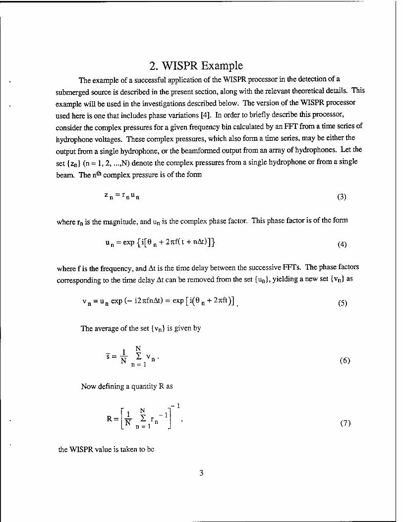
2. WISPR Example The example of a successful application of the WISPR processor in the detection of a

submerged source is described in the present section, along with the relevant theoretical details. This

example will be used in the investigations described below. The version of the WISPR processor

used here is one that includes phase variations [4]. In order to briefly describe this processor,

consider the complex pressures for a given frequency bin calculated by an EFT from a time series of

hydrophone voltages. These complex pressures, which also form a time series, may be either the

output from a single hydrophone, or the beamformed output from an array of hydrophones. Let the

set {zn} (n = 1,2, ...,N) denote the complex pressures from a single hydrophone or from a single

beam. The n* complex pressure is of the form

zn = rnun (3)

where rn is the magnitude, and un is the complex phase factor. This phase factor is of the form

un = exp {i[0 n + 27tf(t + nAt)]} (4)

where f is the frequency, and At is the time delay between the successive FFTs. The phase factors

corresponding to the time delay At can be removed from the set {un}, yielding a new set {vn} as

vn = un exp (- i2jcfnAt) = exp [i(9 n + 27cft)] (5)

The average of the set {vn} is given by

s= N 2 vn. iN n = 1 (6)

Now defining a quantity R as

R = 1 * -l" (7)

the WISPR value is taken to be

W=(R.|s|)2. (8)

The corresponding average WISPR level in decibels is then

W^lOlogW. (9)

The conventional definition of the average power for the set {zn} is

_X N 2 P" N n5jZn' ' (10)

and the corresponding average power level in decibel is

P^ 10 log P. (n)

Having defined the WISPR level (including phase fluctuations) in Eq. (9), it is now

straightforward to calculate the function (PdB - W<IB). For a beam containing a steady tonal such as

that from a submerged source, the WISPR level WdB would be nearly equal to the power level PdB,

and therefore the function (PdB - Wdß) would be nearly zero [1-4]. In contrast, the function (PdB -

Wdß) would have a relatively large positive value for a noise beam [1-4].

The above concepts are illustrated in Fig. 2, showing results from a Pacific experiment which

employed a 144 element hydrophone horizontal line array. The beampattern for the signal in the

frequency bin 5.225 - 5.322 Hz is shown in Fig. 2 (sampling rate: 200 Hz; FFT size: 2048 points;

time series overlap between succssive FFTs: 75%, Hann window). The WISPR level is

approximately 15 dB lower than the average power level on all beams except in the vicinity of beam

number 118, which indicates a steady submerged source by a sudden dip in the difference function

(PdB - Wdß)- It is important to point out that the average power level plot (the top curve) does not

indicate such an unambiguous detection, because it exhibits an even larger peak in the vicinity of

beam number 139, produced by a strong but fluctuating surface source.

3. Variable Time Window Width The effect of varying the width of the time window was studied by repeating the above

calculation using different numbers of DFT points in the initial extraction of amplitudes from the time

series. As in Fig. 2, all calculations reported below focus on the signal in the vicinity of 5.25 Hz,

and use the Hann window. In Fig. 3, the difference function (PdB - Wdß) is plotted along the Y-

axis, and the plots show the effect of decreasing the number of DFT size from 2048 points to 948

points, and to 722 points. In all three cases the signal bin fully contained the signal. (The

importance of this point will become clear by the discussions in Section 4). As the DFT size

decreases, the width of the signal bin correspondingly increase from 0.097 Hz to 0.211 Hz, and to

0.259 Hz, allowing in more noise and causing more fluctuations. As a consequence, the goodness

of detection deteriorated, but only slightly, as indicated by the decreasing dip in the vicinity of beam

number 118. This change is rather small, since the difference function (PdB - W<IB) at beam number

118 changes from approximately 2 dB (for 2048 DFT points) to approximately 5 dB (for 722 DFT

points), in comparison with higher values (approximately 15 dB) for noise beams.

4. Signal Position Within FFT Bin The WISPR level has been observed to be very sensitive to the position of the signal within

the FFT / DFT frequency bin. In order to demonstrate this, we start with Fig. 4 which shows the

average power level of the signal in the vicinity of 5.25 Hz plotted vs. frequency, obtained from

16000 point DFTs. The calculation of Fig. 2 was repeated with DFT sizes 1964,1966,1968,

,1994,1996. Figure 5 shows the upper edges and the lower edges (in frequency space) of the signal

bin in each case, with the plus signs indicating the points at which the DFT calculations were made.

The signal shape of Fig. 4 is marked to scale on the right hand side of Fig. 5. The dashed lines in

Fig. 5 represent the optimum window location as judged from Fig. 7 below.

The average power level PdB, the standard deviation G of the power levels, and the WISPR

level WdB are plotted in Fig. 6 as functions of frequency for DFT sizes 1964,1966,1968, ,

1994,1996. Each frequency value is the median frequency of the signal bin for the

corresponding DFT. The signal shape from Fig. 4 is also shown. The signal bin width is

approximately 0.10 Hz for all the DFTs, and is shown labeled "window size". The average power

level PdB, the standard deviation o of the power levels, the WISPR level WdB, and the difference

function (PdB - Wdß) are shown in greater detail in Fig. 7. The point at approximately 5.295 Hz

corresponds to the 1964 point DFT, and the point at approximately 5.21 Hz corresponds to the 1996

point DFT. An examination of the signal shape and the signal bin width in Fig. 6 reveals that for the

5

1964 point DFT (5.295 Hz) and for the 1996 point DFT (5.21 Hz), small portions of the signal

energy lie outside the signal bin. In spite of this, the average power levels at these points differ only

less than 1 dB from their peak value which occurs at approximately 5.25 Hz (Fig. 7). However, the

WISPR level is significantly affected, and it changes by as much as 5 dB from its peak level

(Fig. 7). Since the smallness of the difference function is the criterion for detection of stable signal

sources, it is clear that WISPR detection capability deteriorates when even a small portion of the

signal energy falls outside the signal bin, as at 5.295 Hz and at 5.21 Hz.

The above observations are confirmed by the results in Figure 8(a), which shows the upper

edges and the lower edges of the signal bin for DFT sizes 948,972,986, and 1024. The dashed

lines represent the optimum window location as judged from Fig. 7. Clearly portions of the signal

energy for the 972 point DFT falls outside the signal bin for this case. Figure 8(b) shows that the

corresponding WISPR level is about 14 dB lower than the other WISPR levels where the complete

signal energy falls within the signal bin. In contrast, this variation has only a miniscule effect on the

average power.

5. Conclusions The foregoing analysis demonstrates that variable width of the time series window in FFT /

DFT calculations has only a small effect on WISPR performance, provided that the full signal energy

is contained within the signal bin. When the signal position within the signal bin is such that a small

portion of the signal energy falls outside the signal bin, the average power level is only slightly

affected. However, such loss of even a small portion of the signal energy from the signal bin has a

dramatic effect on the WISPR level, and causes deterioration in WISPR performance by several

decibels. Therefore, in applications of wavelet transforms to WISPR processing, special care must

be taken to ensure that the signal bin contains the full signal energy, and that no portion of this

energy falls in adjacent bins.

The most effective ways to do WISPR processing accurately when the signal energy

necessarily has to fall in at least two or more frequency bins due to small bin width, is a topic that

remains to be investigated.

The sensitivity of the WISPR level to the signal position within the signal bin can be used to

determine the signal frequency more precisely, avoiding the necessity to carry out calculations using

much larger data sets.

6

6. Acknowledgments This work was performed under the Program Element number PE0602435N, and was

supported by the Office of Naval Research, Mr. Tommy Goldsberry, Program Manager.

References [1] R. A. Wagstaff, "The WISPR filter: A method for exploiting fluctuations to achieve improved

sonar signal processor performance," (submitted to J. Acoust. Soc. Am.)

[2] J. George and R. A. Wagstaff, "Variations of WISPR levels and average power levels with

standard deviation," NRL Memorandum Report No. NRL/MR/7176--93-7077 (1994).

[3] J. George and R. A. Wagstaff, "WISPR performance measured by ROC curves," NRL

Memorandum Report No. NRL/MR/7176-94-7559 (1994).

[4] R. A. Wagstaff and J. George, "A new fluctuation based processor including phase variations",

(to be submitted to J. Acoust. Soc. Am.)

[5] C. K. Chui, An Introduction to Wavelets, (Academic, New York, 1992), Ch. 3.

[6] H. H. Szu, B. Telfer, and A. Lohmann, "Causal analytical wavelet transform", Optical Eng. 3_I,

1825 (1992)

[7] M. Badiey, I. Jaya, and A. H. D. Cheng, "Shallow water acoustic/geoacoustic experiments at

the New Jersey Atlantic generating station site," J. Acoust. Soc. Am. 96, 3593-3604 (1994).

[8] D. M. Drumheller, et.al., "Identification and synthesis of acoustic scattering components via the

wavelet transform," J. Acoust. Soc. Am. 97, 3649-3656 (1995).

Figure Captions Figure 1. Comparison of the results of time-frequency analyses using (a) the "short-time Fourier

transform", and (b) the Morlet transform (from Ref. 7).

Figure 2. The beampattern for the signal (including noise) in the frequency bin 5.225 - 5.322 Hz

from a Pacific experiment employing a 144 hydrophone horizontal line array (sampling rate:

200 Hz; FFT size: 2048 points; Hann window). The average power level, the WISPR level,

and the difference between the two are labeled.

Figure 3. The effect of varying the size of time window on WISPR performance. The difference

function (PdB - Wdß) is plotted along the Y-axis.

Figure 4. The average power level of the signal in the vicinity of 5.25 Hz plotted vs. frequency,

obtained from 16000 point DFTs.

Figure 5. The upper edges and the lower edges of the signal bin for DFT sizes 1964,1966,1968,

, 1994,1996. The plus signs indicate the points at which the DFT calculations were

made. The dashed lines represent the optimum window location as judged from Fig. 7.

Figure 6. The average power level PdB, the standard deviation a of the power levels, and the

WISPR level WdB plotted as functions of frequency for DFT sizes 1964,1966,1968, ,

1994,1996. Each frequency value is the median frequency of the signal bin for the

corresponding DFT. The plus signs indicate the points at which the DFT calculations were

made.

Figure 7. The average power level PdB, the standard deviation O" of the power levels, the WISPR

level WdB, and the difference function (PdB - Wdß) plotted as functions of frequency for DFT

sizes 1964, 1966, 1968, , 1994,1996. Each frequency value is the median frequency

of the signal bin for the corresponding DFT. The plus signs indicate the points at which the

DFT calculations were made.

Figure 8(a): The upper edges and the lower edges of the signal bin for DFT sizes 948,972,986,

and 1024. The plus signs indicate the points at which the DFT calculations were made. The

dashed lines represent the optimum window location as judged from Fig. 7. Fig. 8(b): The

average power level PdB, the standard deviation a of the power levels, and the WISPR level

WdB, for DFT sizes 948, 972, 986, and 1024.

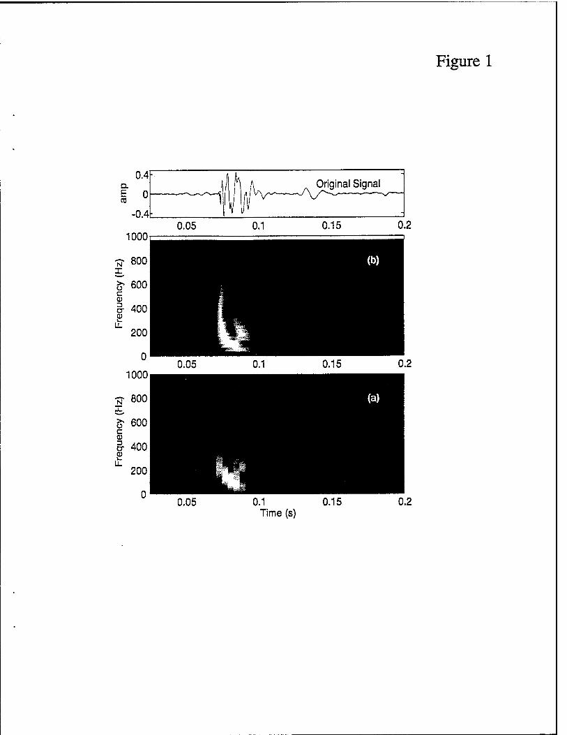
Figure 1

0.05 0.1 Time (s)

0.15

Figure 2

PQ

>

o

100

80

60

40

20

-i—i—i—i—i—i—i i i r

'_ Avpower level: PdB

-T 1 ]—i—i—-t i r ^ i i *

0

WISPR level: WdB

(PdB " WdB) oL_ _i ! I

50 100 150 BEAM#

200 250

Figure 3

PQ

40 h 722 point DFT Bin width: 0.259 Hz

250

>

CO

>

o 40 h

20

0 0

948 point DFT Bin width: 0.211 Hz

250

2048 point DFT Bin width: 0.097 Hz

50 100 150 BEAM#

200 250

Figure 4

5F -i—i—i—r • i i

m

cc LU

O

> <

o-

-5

•10

■15

-20 ' ' L_

5.20 5.22 5.24 5.26 FREQ (Hz)

5.28 5.30

Figure 5

5.40 ~"i—:—i—i—i—i—i—i—i—]—i—i—i—i—i—i—i—i—i—|—i—i—i—i—i—i—:—i—i—|—i—i—r i i i i

l

l

l

: -f-s^Window upper edge -

5.30

5.20

— ^~*"S K^,

^Signal i shape :

N 1

/

i i

i i

i i

i

o LU

— ^ 1—K_.

tr LL : Window lower edge -

5.10 - -

5.00 j.i.iitiiiiiiiiii-i!,!,. i..j..i...j._i j j l_t—i—:—i—i—i—•_

1960 1970 1980 1990 2000 NDFT

2010

Figure 6

ior ->—i—i—r -i 1 1 r -t——i i r

HI

cc UJ

5 o CL

0

-5

•10

■15

•20 5.15

Window size / * * r

a

^-PdB

WdB

Signal shape

i , •

5.20 5.25 5.30 FREQ (Hz)

5.35

Figure 7

10

CQ

LU

o CL

"»K.

. Std. dev.'a""::+':

0

-10

-1 1 1 1 i r -1 1 [ 1 1 r

(PdB-WdB)/ :

Avpower level: PdB 4. —

WISPR level:

5.20 5.22 5.24 5.26 FREQ (Hz)

5.28 5.30

Figure 8

CD

d LU

o

10F

5

0

-5

-10

-15

-20

-i—i—.—r -1 1 T- -i 1 r- -1 1 r

+-• «4 Std. dev. a .i +

Ävpower level: PdB

WISPR level: WdB

(b) -

940 960 980 1000 1020 1040 NDFT

5.6

N IE

5,4

a LU CC

^ 5.2

5.0

-T—:—i—|—i—i—i—i—i—i—"—| ' ' ' r -l 1 ] 1 1 r-

Window upper edge

Window lower edge

' ' I I L.

(a)

Signal shape

_i i—i—i-

940 960 980 1000 1020 1040 1060 NDFT