Embed Size (px)
Citation preview
Qual QuantDOI 10.1007/s11135-013-9984-4
The effects of trade liberalization on environmentaldegradation
Shu-Chen Chang
© Springer Science+Business Media Dordrecht 2013
Abstract This paper uses a threshold model to estimate the regime-specific marginal effectof trade liberalization and other determinants of environmental degradation in regimes withdifferent levels of corruption. The results show that increasing trade liberalization leads toan increase in carbon dioxide (CO2) emissions in countries with a high level of corruptionbut to an decrease in countries with low corruption. A U-shaped relationship between CO2
emissions and income exists in low-corruption countries but not in high-corruption countries.Our results also show that an increase in energy use per $1,000 in gross domestic productand fossil-fuel energy consumption will increase CO2 emissions in any country. Moreover,increases in agricultural value and foreign direct investment can decrease environmentaldegradation in any country.
Keywords Pollution · Threshold effect · Trade liberalization
1 Introduction
Trade liberalization has become the center of attention in empirical analysis of environmentaldegradation since the implementation of the North American Free Trade Agreement (NAFTA)in 1994. Increasing evidence supports the hypothesis that trade liberalization is one of thefundamental determinants of environmental degradation. According to economic theory,trade liberalization has contradictory effects. For example, when pollution is an inferior good(i.e., the income elasticity of pollution is negative), trade liberalization induces income growthand encourages people to increase demand for a clean environment. But when pollution is anormal good (i.e., the income elasticity of pollution is positive), trade liberalization causesenvironmental quality to deteriorate because it increases the scale of economic activity.
From another point of view, institutional quality is critical in analyzing these contradic-tory empirical results. Due to economic integration, governments are under pressure from
S.-C. Chang (B)Department of Business Administration, National Formosa University, Yunlin, Taiwane-mail: [email protected]
123
S.-C. Chang
environmental lobby groups and industry to change their environmental policy. A few stud-ies (Bommer and Schulze 1999; Copeland 2005; Damania et al. 2003; Lai 2006) point outthat the environmental policy under a corrupt government is affected by bribes from produc-ers. Low-corruption governments are likely to provide good-quality environmental policies,while few high-corruption governments are likely to do so. Institutional quality can be animportant variable in empirical studies examining trade liberalization and environmentaldegradation.
Empirical studies that include data on institutional quality found a correlation betweenmeasures of institutional quality, trade, and the environment. Antweiler et al. (2001) showthat pollution policy varies with economic conditions and the type of government, whichcares about the environment to a greater or lesser extent. Later, Damania et al. (2003) use theinteraction between trade, government corruption, and environmental pollution to explore theeffect of trade liberalization on the environment. They show that the effect of import dutieson lead content in gasoline decreases as the value of the government honesty index increases(i.e., corruption falls), implying that corruption increases the effect of trade liberalization onlead content in gasoline. Copeland’s (2005) study points out that it may be misleading toassume that trade is good for the environment. He provides a set of theoretical concepts toanalyze this possibility and shows that good-quality government leads to cause both moreopenness and positive environmental outcomes, while more openness worsens environmentalquality. In addition, Forslid et al. (2013) build a monopolistic competition trade model andpoint out that trade liberalization increases global emissions when market sizes are symmetricand taxes are different. Thus, the effect of trade liberalization on environmental policy dependson the level of corruption.
This line of research thus far has focused on the creation of environmental degradation,using trade as one of the explanatory variables. In contrast to previous studies, the presentpaper focuses on actual pollution as the dependent variable in a linear regression. The level ofactual pollution depends on the effectiveness of law enforcement, which varies with institu-tional quality. This paper is the first to examine the relationship between trade liberalizationand environmental degradation. In contrast to related studies, this paper focuses on whetherthe relationship between trade liberalization and environmental degradation is contingenton the quality of political institutions. This paper tests for a threshold level of corruption atwhich the effect of trade liberalization on environmental degradation changes from negativeto positive, as corruption surpasses that level.
Following most of the empirical literature on threshold effects, the paper utilizes theCaner and Hansen’s (2004) threshold regression. Compared to regression with an interactionterm, threshold regression has the advantage that its approach allows all parameters of theenvironmental degradation model to differ across regimes and to be discretely different.Furthermore, this approach can identify the regimes and estimate the environmental effects oftrade liberalization in a particular governance regime. When considering the environmentaleffect of trade liberalization as dependent on the quality of political institutions (politicalquality), political quality is treated as a threshold variable to define governance regimesand to estimate the regime-specific marginal effect of trade liberalization on environmentaldegradation in different regimes.
This study contributes to the research by using a threshold model for environmental degra-dation to investigate the environmental policy debate on whether an environmental effect oftrade liberalization exists. In addition, we investigate and analyze the possible existence of aregime-specific relationship between environmental degradation and trade liberalization inmultiple political quality regimes. The paper differs from previous papers in two respects:(1) environmental degradation and trade liberalization are jointly determined within a
123
The effects of trade liberalization
particular governance regime; (2) the margin impact of corruption and other determinants ofenvironmental degradation is regime specific.
The rest of the study is organized as follows. Section 2 is a literature review. Section 3describes the conceptual and empirical model. Section 4 gives a description of the vari-ables. Section 5 gives data sources and the estimation results. The economic implications areanalyzed in Sect. 6, and concluding remarks are given in Sect. 7.
2 Literature review
In early studies, Grossman and Krueger (1993) investigate the environmental impacts ofNAFTA. Grossman and Krueger’s (1993) study supports an income effect: that trade lib-eralization tends to improve environmental quality via income growth. Is trade good forthe environment? In subsequent studies, Gale and Mendez (1998) find that an increase inincome has a negative effect on environmental quality, but the effect of trade on pollution isinsignificant. Antweiler et al. (2001) divide trade’s impact on pollution into scale, technique,and composition effects and find that trade openness creates relatively small increases inpollutant emissions when it alters the composition of national output. On the contrary, tradeopenness reduces pollution through technique and scale effects. Antweiler et al. (2001) com-bine the overall effects and conclude that freer trade appears to be good for the environment.Furthermore, Dean (2002) shows that trade liberalization has not only an indirect but alsoa direct effect on environmental degradation. The direct effect is a trade-induced changein emissions from the composition of industries, and the indirect effect is a trade-inducedchange in emissions from income.
In a related line of empirical work, previous studies use different indicators of pollutionto measure environmental degradation and have different findings. Antweiler et al. (2001),Frankel and Rose (2005), and Harbaugh et al. (2002) all use air quality to proxy environ-mental degradation and find that trade openness has a positive impact on air quality. Dean(2002) uses Chinese provincial data on water pollution and finds that trade has the effect ofreducing water pollution. Lucas et al. (1992) use cross-sectional data for a group of devel-oping and industrialized countries and apply toxic intensity, measured by the compositionof manufacturing output, to proxy environmental damage. Lucas et al. find that increases intrade openness reduce the growth of toxic intensity.
Extending previous literature on the environmental effect of trade, Fredriksson (1999)finds that, in a perfectly competitive sector, trade liberalization decreases (increases) bothindustrial and environmental lobby groups’ incentive to influence environmental policy if thecountry has a comparative disadvantage (advantage) in the polluting sector (Damania et al.2003). Bommer and Schulze’s (1999) finding also shows that governments prefer to provideweak (strict) environmental policy when trade is liberalized if the import-competing sector(export sector) is pollution intensive. The result of Fredriksson’s (1999) study seems thatthe environmental effect of trade liberalization depends on the relative strength of politicalpressure.
Copeland (2005) points out that if the quality of the government is good, both more opentrade and a cleaner environment will result, however, if the quality of the government is poor,more open trade may well worsen environmental quality. Damania et al. (2003), based on 48countries from 1982 to 1992, investigate the linkages between trade policy, corruption, andenvironmental policy and find that the effect of trade liberalization on environmental policydepends on the level of corruption. Forslid et al. (2013) develop a monopolistic competitiveframework to study the impact of trade liberalization on local and global emissions. Forslid
123
S.-C. Chang
et al. show that trade liberalization leads to lower global emissions in countries with a largemarket and high tax on emissions. Generally, our results suggest that relative market size, thelevel of trade costs, the ease of pollution abatement, and the degree of product differentiationat the sectoral level are relevant variables for empirical studies on trade and pollution.
Recently, several studies (Aidt et al. 2008; Bose et al. 2008) have used the quality ofpolitical institutions as a threshold variable. Aidt et al. (2008) and Bose et al. (2008) usea governance indicator and Transparency International’s (TI) corruption perceptions index(CPI) as a threshold variable in an economic growth model and a quality of public insti-tutions model, respectively. Extending measures of threshold variables from these studiesverifies the notion that the government is willing to allow lobbying groups to influence theprocess of environmental policy formation. According to related theoretical work, includ-ing Damania et al. (2003), Fredriksson (1999), Hillman and Ursprung (1994), and Rauscher(1994), lobbying incentives influence trade reform and have a further impact on environmen-tal quality. In addition, several studies (Coates 1996; Helland 1998; Pashigian 1985) find thatpolitical economy pressures are important determinants of environmental policy. These stud-ies also show that reducing the level of corruption can create greater social welfare and leadto an increase in the emissions tax. Thus, the effect of trade liberalization on environmentaldegradation depends on the level of corruption.
Although these previous studies consider the role of corrupt governments in trade liber-alization’s effect on pollution, they do not consider the problem of the endogeneity of trade.Trade should be treated as endogenous rather than exogenous because it can be influencedby trade freedom, human capital, the stock of physical capital, and basic infrastructure. Inaddition, Copeland (2005) points out that the “government prefers to protect polluters withtariffs than with weak pollution policy when trade policy is endogenous because it imposesless cost on consumers.”
3 Theoretical framework and empirical model
3.1 Theoretical framework
The environmental effects of trade liberalization and other measures of economic activityrely on a theoretical framework developed by Copeland (2005), Copeland and Taylor (2004),and Forslid et al. (2013). Following Copeland and Taylor (2004) and Forslid et al. (2013),firms produce two outputs: an industrial good (x) and emissions (e). This paper considers twoidentical countries: home and foreign countries. There are n firms in each country, and n ≥ 1.All firms produce a homogeneous good and face a constant marginal cost of production.
Let C(x j ) be the production cost function of a firm in country j . The cost function isassumed to be strictly increasing (C ′(x j ) > 0) and convex (C ′′(x j ) > 0). According toForslid et al. (2013) study, the cost function of a firm in country j is given by
C(x j ) = F + k j tαj x j , (1)
where k = α−α(1 − α)(1−α). F is the fixed cost. t is the tax on emissions, which is leviedby the government to control emissions. Using Shepard’s Lemma on the cost function(i.e., Eq. (1)) derives a firm’s demand for emissions in country j ,
e j = ∂C(x j )
∂t j= αktα−1
j x j (2)
123
The effects of trade liberalization
As Eq. (2) shows, increases in the emissions tax, t , will decrease firms’ emissions. In addition,increases in efficient abatement technology (i.e., lower α) also will decrease firms’ emissionsas α−1 is a measure of the effectiveness of abatement technology.
The optimal output of good x for a firm in country j can be obtained by Hotelling’s Lemmaas follows (Forslid et al. 2013)
x∗j = F(σ − 1)
ktαj(3)
In addition, total emissions from firms in the home and foreign country are as follows,respectively1 (Forslid et al. 2013),
Eh = α(σ − 1)μθ{((1 − s)ϕ2 + s)T α(σ−1) − ϕ
}
σ th{1 − ϕT α(σ−1)
} {T α(σ−1) − ϕ
} (4)
E f = α(σ − 1)μθT α(σ−1){(1 − (1 − ϕ2)s − ϕT α(σ−1)
}
σ t f{1 − ϕT α(σ−1)
} {T α(σ−1) − ϕ
} , (5)
where ϕ denotes trade liberalization because of ϕ = τ 1−σ , where τ and σ are the tradedcost and the elasticity of substitution, respectively. T is relative emission taxes between thehome and foreign country. σ, θ, μ, and s are parameters, in which θ ∈ (0, 1) , μ ∈ (0, 1),and s ∈ (0, 1).
When market size, s, and emissions taxes, t , differ between the home and foreign country,the change in globally environmental degradation due to a change in trade liberalization, ∂ E
∂ϕ,
is as follows
∂ E
∂ϕ=α(σ − 1)μθϕT α(σ−1)(T − 1)
s(T α(σ−1)−ϕ)2 − (1 − s)(T α(σ−1)ϕ − 1)2
σ t f (1 − ϕT α(σ−1))2(T α(σ−1) − ϕ)2, (6)
where the sign of ∂ E∂ϕ
depends on emissions taxes and market size. When (T α(σ−1) − ϕ)2 ≥(T α(σ−1)ϕ − 1)2 for T > 1, and s > (1 − s) for s > 1
2 , ∂ E∂ϕ
> 0. However, the effect oftrade liberalization on globally environmental degradation will be ambiguous when T < 1and s > 1
2 .Previous studies (Damania et al. 2003) point out that the lobbying groups pay bribes to
environmental policymakers and thus influence the process of environmental policy forma-tion. Copeland (2005) suggests that pollution policy depends on factors such as how corruptthe government is. Following Damania et al. (2003), this paper assumes the utility of gov-ernment function as follows
G(t, τ ) = S(t) + βW (t, τ ), (7)
where W (t, τ ) is aggregate social welfare and S(t) is return on bribes received.β is the degreeof corruptibility, and β > 0.
According to Damania et al. (2003) study, deviating from Eq. (7) can obtain the changein global environmental degradation due to a change in the degree of corruption,
∂t
∂β= −∂W (t∗)/∂t
∂2G/∂t2 , (8)
where ∂W (t∗)/∂t > 0 and ∂2G(t∗)/∂t2 < 0.
1 The details the deviation please see Forslid et al. (2013).
123

S.-C. Chang
When β → ∞, bribes become relatively less important (i.e., low corruption), and then thedistortion of environmental policy declines. Thus, increases in corruption reduce the pollutiontax. Because Eqs. (6) and (8) show the effect of trade liberalization on pollution as dependingon the market size and the degree of corruption, the implications offer an opportunity forbringing some empirical clarity to the identified threshold effects. Thus, the reduced form ofthe pollution model is as follows
Qi ={
′1T Li + ′
1ωi + ε1i ; q ≤ γ
′2T Li + ′
2ωi + ε2i ; q ≥ γ(9)
In Eq. (9), Qi indicates environmental degradation. T Li indicates trade liberalization. Vari-able ωi is a set of control variables that include variables for economic activities. Variable qi
is an exogenous threshold variable. This paper uses the degree of corruption as a thresholdvariable. is the threshold value to be estimated. εi is a disturbance term. In Forslid et al.(2013) study, trade liberalization influences environmental pollution, but trade liberalizationis correlated with trade costs. That is, trade liberalization should be treated as endogenous.
Damania et al. (2003) empirical work uses grams of lead content per gallon of gasoline as aproxy for environmental policy and shows the effect of trade liberalization on environmentalpolicy depending on the level of corruption. Most studies adopt CO2 emissions as a proxy forenvironmental degradation or pollution (Talukdar and Meisner 2001; Tamazian et al. 2009;Tamazian and Rao 2010). Thus, this paper uses CO2 emissions as a proxy for environmentaldegradation. Theoretical models demonstrate a relationship between emissions and trade.
3.2 Empirical model
The effect of income per capita on environmental quality has been taken into account byenvironmental policymakers, but not the trade liberalization effect. Most studies show thatthe relationship between income per capita and environmental pollution is a nonmonotonicrelationship (Brock and Taylor 2005). The nonmonotonic relation is that pollution first risesand then falls with growth in income per capita. Explanations for this relation generallyfocus on three primary factors (i.e., income growth, technological progress, and changesin the composition of aggregate output) that interact to produce its shape. To reduce theunexplained variation in the estimation process, our empirical model includes various controlvariables. Extending Eq. (9), the environmental degradation model is rewritten as follows:
Qi = ′1
[T Li
ωi
]I (qi ≤ γ ) + ′
2
[T Li
ωi
]I (qi > γ ) + ei , (10)
where ω′i = (Yi , Y 2
i , F F Ei , AGi , E Ei , F DIi ).All variables in Eq. (10) are explained in Table 1.In Eq. (10), income per capita, Yi , is used to capture the scale effect to reflect the impact of
increasing (or decreasing) growth in income per capita on environmental degradation, holdingconstant the mix of sectors and technology. This paper adds a squared term of income percapita (Y 2
i ) to acknowledge the existence of the environmental Kuznets curve. The ratio ofagricultural value added to agricultural value added to (GDP) (AGi ) is used as a proxy forthe composition effect and reflects changes in the sectoral structure of an economy, holdingconstant the scale and technology. The ratio of net foreign direct investment (FDI) to GDP(F DIi ) is used as a proxy for the technology effect as well as to reflect energy efficiency,holding constant the scale and the mix of sectors.
123
The effects of trade liberalization
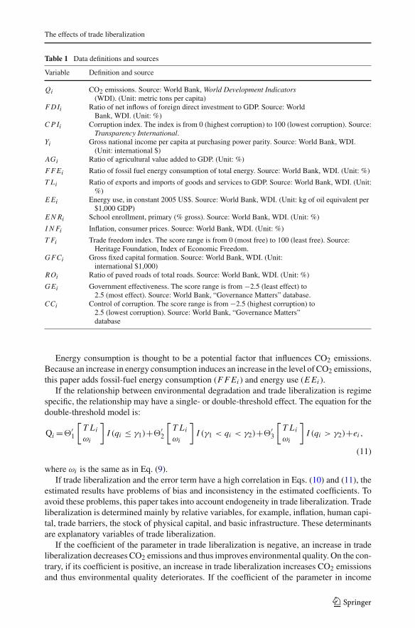
Table 1 Data definitions and sources
Variable Definition and source
Qi CO2 emissions. Source: World Bank, World Development Indicators(WDI). (Unit: metric tons per capita)
F DIi Ratio of net inflows of foreign direct investment to GDP. Source: WorldBank, WDI. (Unit: %)
C P Ii Corruption index. The index is from 0 (highest corruption) to 100 (lowest corruption). Source:Transparency International.
Yi Gross national income per capita at purchasing power parity. Source: World Bank, WDI.(Unit: international $)
AGi Ratio of agricultural value added to GDP. (Unit: %)
F F Ei Ratio of fossil fuel energy consumption of total energy. Source: World Bank, WDI. (Unit: %)
T Li Ratio of exports and imports of goods and services to GDP. Source: World Bank, WDI. (Unit:%)
E Ei Energy use, in constant 2005 US$. Source: World Bank, WDI. (Unit: kg of oil equivalent per$1,000 GDP)
E N Ri School enrollment, primary (% gross). Source: World Bank, WDI. (Unit: %)
I N Fi Inflation, consumer prices. Source: World Bank, WDI. (Unit: %)
T Fi Trade freedom index. The score range is from 0 (most free) to 100 (least free). Source:Heritage Foundation, Index of Economic Freedom.
G FCi Gross fixed capital formation. Source: World Bank, WDI. (Unit:international $1,000)
ROi Ratio of paved roads of total roads. Source: World Bank, WDI. (Unit: %)
G Ei Government effectiveness. The score range is from −2.5 (least effect) to2.5 (most effect). Source: World Bank, “Governance Matters” database.
CCi Control of corruption. The score range is from −2.5 (highest corruption) to2.5 (lowest corruption). Source: World Bank, “Governance Matters”database
Energy consumption is thought to be a potential factor that influences CO2 emissions.Because an increase in energy consumption induces an increase in the level of CO2 emissions,this paper adds fossil-fuel energy consumption (F F Ei ) and energy use (E Ei ).
If the relationship between environmental degradation and trade liberalization is regimespecific, the relationship may have a single- or double-threshold effect. The equation for thedouble-threshold model is:
Qi =′1
[T Li
ωi
]I (qi ≤ γ1)+′
2
[T Li
ωi
]I (γ1 < qi < γ2)+′
3
[T Li
ωi
]I (qi > γ2)+ei ,
(11)
where ωi is the same as in Eq. (9).If trade liberalization and the error term have a high correlation in Eqs. (10) and (11), the
estimated results have problems of bias and inconsistency in the estimated coefficients. Toavoid these problems, this paper takes into account endogeneity in trade liberalization. Tradeliberalization is determined mainly by relative variables, for example, inflation, human capi-tal, trade barriers, the stock of physical capital, and basic infrastructure. These determinantsare explanatory variables of trade liberalization.
If the coefficient of the parameter in trade liberalization is negative, an increase in tradeliberalization decreases CO2 emissions and thus improves environmental quality. On the con-trary, if its coefficient is positive, an increase in trade liberalization increases CO2 emissionsand thus environmental quality deteriorates. If the coefficient of the parameter in income
123
S.-C. Chang
per capita is negative (positive), an increase in income per capita decreases (increase) CO2
emissions and thus improves environmental quality. If the coefficient of income per capitaand its square are positive and negative, respectively, it indicates the presence of an invertedU-shape. If the coefficients of fossil-fuel use and energy use are positive, it means that anincrease in fossil-fuel use and energy use increases CO2 emissions and thus environmentalquality deteriorates. If the coefficients of agricultural value and FDI inflows are negative, itmeans that an increase in agricultural value and FDI inflows could decrease CO2 emissionsand thus improve environmental quality.
3.3 Estimation and tests
The estimation of the environmental pollution model involves the following procedure. First,this paper determines whether the instrumental variable is valid. In order to validate theseinstruments, we performed a test of weak instruments based on the Wald statistic of Craggand Donald (1993) (see Stock and Yogo 2005). The Wald statistic test is used for the nullhypothesis that a given group of instruments is weak.
Second, this paper finds threshold values by minimizing the sum of the squared residualsgiven the presence of threshold effects. Third, we test whether the environmental degradationmodel has nonlinearity. The null hypothesis of no threshold effects is H0 :1 =2, and thetest for H0 is the Sup Wald statistic proposed by Davies (1987). The Sup Wald statistic forno threshold can be represented by
SupW = supγ∈�
Wn(γ). (12)
The asymptotic p values of the statistic SupW can be calculated with arbitrary accuracy byrepeated simulations using Hansen’s (1996) extended approach. Hansen’s (1996) bootstrapp values are computed for each γ . Thus the bootstrap p value is
p̂∗(γ) = 1
B
B∑
j=1
I(SupW∗j > SupW), (13)
where I(.) is the indicator function, which equals 1 if its argument is true and 0 otherwise.The simulated p value is the fraction of time such that SupW∗
j is smaller than SupW. Finally,we determine the number of thresholds after the threshold effect is proved.
4 Description of variables
4.1 Environmental degradation
We use CO2 emissions as the environmental degradation measure for several reasons. Themain reason is that CO2 has been recognized as a major source of global warming through itsgreenhouse gas effects because it is emitted from burning fossil fuels and industrial processes.Hence, it has severe effects on the natural environment (e.g., it contributes to global warming).In addition, regulating and monitoring CO2 emissions from various economic activities havebecome a central issue in ongoing negotiations over an international treaty on global warming(Revkin 2000). Another reason is that CO2 emissions are directly related to the use of energy,which is an essential factor in the world economy, for both production and consumption.
The final reason is that among the principal air pollutants, CO2 is the major measure ofair pollution and has been widely used in empirical studies. Data on CO2 emissions can
123
The effects of trade liberalization
be obtained from Carbon Dioxide Information Analysis Center at the Oak Ridge NationalLaboratory.2
4.2 Trade liberalization
Liberalization of trade in an economy is difficult to quantify, therefore, most studies usevarious instruments to measure it. Generally, instruments that measure trade liberaliza-tion comprise openness in practice (which is called openness of outcome) and opennessof policy. The former is related to the actual degree of trade openness, but the latter isrelated to trade policy. Direct quantification of openness of outcome can be seen in theactual trade flows. Direct measurement of openness of policy comprises trade restrictionssuch as tariffs, quotas, and duty exemption schemes. However, measuring trade restrictionsis difficult because of the lack of agreed definitions and available databases. In contrast,data on actual trade flows are available from the World Bank database, and these data haveagreed definitions. For the above reasons and facilitating empirical investigation, opennessin the actual degree of trade flows is used as a suitable proxy for trade liberalization in thispaper.
It is worth mentioning that actual trade flows are the result not only of trade policy but alsonatural conditions and costs, absolute and relative to trading partners, and macroeconomicconditions. Therefore, in this paper, trade liberalization is considered as an endogenousvariable, which can be influenced by trade freedom, human capital, the stock of physicalcapital, inflation, basic infrastructure, and so on.
Actual trade flows are the value of total trade (imports plus exports) as a percentage ofGDP. The data on actual trade flows come from the World Development Indicators (WDI)published by World Bank.
4.3 Corruption
Corruption index data come from Transparency International (TI). Because TI publisheshistorical data annually, the index of corruption constructed in the TI is used in this study.The index uses a scale from 0 to 100, where a score of 100 indicates very little corruptionand a score of 0 indicates a very corrupt government.
If corruption has an impact on the rule of law system, rent-seeking firms will have lessinfluence on environmental policy under this system. Thus, the less corrupt system promotesa more stringent environmental policy and decreases environmental degradation.
5 Data sources and estimation results
5.1 Data sources
This paper uses cross-sectional data for 51 countries (see Appendix Table 10) for the periodfrom 1997 to 2007 to examine the nonlinear relationship between environmental degradationand trade liberalization. All data are averaged for the period from 1997 to 2007. Our datacome from the World Bank database, except for trade freedom data (which come from theIndex of Economic Freedom of the Heritage Foundation) and CPI data (which is from theTI). CPI is the measured corruption index, where 100 is the lowest level of corruption and 0 is
2 Data source: http://cdiac.ornl.gov.
123
S.-C. Chang
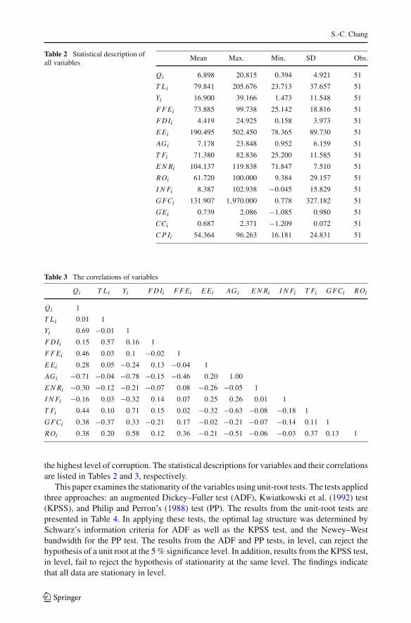
Table 2 Statistical description ofall variables
Mean Max. Min. SD Obs.
Qi 6.898 20.815 0.394 4.921 51
T Li 79.841 205.676 23.713 37.657 51
Yi 16.900 39.166 1.473 11.548 51
F F Ei 73.885 99.738 25.142 18.816 51
F DIi 4.419 24.925 0.158 3.973 51
E Ei 190.495 502.450 78.365 89.730 51
AGi 7.178 23.848 0.952 6.159 51
T Fi 71.380 82.836 25.200 11.585 51
E N Ri 104.137 119.838 71.847 7.510 51
ROi 61.720 100.000 9.384 29.157 51
I N Fi 8.387 102.938 −0.045 15.829 51
G FCi 131.907 1,970.000 0.778 327.182 51
G Ei 0.739 2.086 −1.085 0.980 51
CCi 0.687 2.371 −1.209 0.072 51
C P Ii 54.364 96.263 16.181 24.831 51
Table 3 The correlations of variables
Qi T Li Yi F DIi F F Ei E Ei AGi E N Ri I N Fi T Fi G FCi ROi
Qi 1
T Li 0.01 1
Yi 0.69 −0.01 1
F DIi 0.15 0.57 0.16 1
F F Ei 0.46 0.03 0.1 −0.02 1
E Ei 0.28 0.05 −0.24 0.13 −0.04 1
AGi −0.71 −0.04 −0.78 −0.15 −0.46 0.20 1.00
E N Ri −0.30 −0.12 −0.21 −0.07 0.08 −0.26 −0.05 1
I N Fi −0.16 0.03 −0.32 0.14 0.07 0.25 0.26 0.01 1
T Fi 0.44 0.10 0.71 0.15 0.02 −0.32 −0.63 −0.08 −0.18 1
G FCi 0.38 −0.37 0.33 −0.21 0.17 −0.02 −0.21 −0.07 −0.14 0.11 1
ROi 0.38 0.20 0.58 0.12 0.36 −0.21 −0.51 −0.06 −0.03 0.37 0.13 1
the highest level of corruption. The statistical descriptions for variables and their correlationsare listed in Tables 2 and 3, respectively.
This paper examines the stationarity of the variables using unit-root tests. The tests appliedthree approaches: an augmented Dickey–Fuller test (ADF), Kwiatkowski et al. (1992) test(KPSS), and Philip and Perron’s (1988) test (PP). The results from the unit-root tests arepresented in Table 4. In applying these tests, the optimal lag structure was determined bySchwarz’s information criteria for ADF as well as the KPSS test, and the Newey–Westbandwidth for the PP test. The results from the ADF and PP tests, in level, can reject thehypothesis of a unit root at the 5 % significance level. In addition, results from the KPSS test,in level, fail to reject the hypothesis of stationarity at the same level. The findings indicatethat all data are stationary in level.
123
The effects of trade liberalization
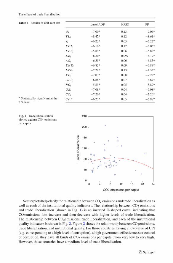
Table 4 Results of unit-root test
∗ Statistically significant at the5 % level
Level ADF KPSS PP
Qi −7.00* 0.13 −7.06*
T Li −8.47* 0.12 −8.61*
Yi −6.23* 0.05 −6.22*
F DIi −6.10* 0.12 −6.05*
F F Ei −5.89* 0.06 −5.82*
E Ei −6.30* 0.097 −6.19*
AGi −6.59* 0.06 −6.85*
E N Ri −6.85* 0.09 −6.89*
I N Fi −7.29* 0.13 −7.33*
T Fi −7.03* 0.08 −7.22*
G FCi −6.86* 0.07 −6.87*
ROi −5.89* 0.05 −5.89*
G Ei −7.08* 0.04 −7.08*
CCi −7.20* 0.04 −7.20*
C P Ii −6.25* 0.05 −6.98*
Fig. 1 Trade liberalizationplotted against CO2 emissionsper capita
0
40
80
120
160
200
240
0 4 8 12 16 20 24
CO2 emissions per capita
Tra
de li
bera
lizat
ion
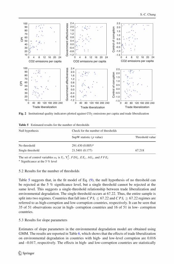
Scatterplots help clarify the relationship between CO2 emissions and trade liberalization aswell as each of the institutional quality indicators. The relationship between CO2 emissionsand trade liberalization (shown in Fig. 1) is an inverted U-shaped curve, indicating thatCO2emissions first increase and then decrease with higher levels of trade liberalization.The relationship between CO2emissions, trade liberalization, and each of the institutionalquality indicators is shown in Fig. 2. Figure 2 shows the relationship between CO2emissions,trade liberalization, and institutional quality. For those countries having a low value of CPI(e.g. corresponding to a high level of corruption), a high government effectiveness or controlof corruption, they have all kinds of CO2 emissions per capita, from very low to very high.However, those countries have a medium level of trade liberalization.
123
S.-C. Chang
102030405060708090
100
0 4 8 12 16 20 24
CO2 emissions per capita CO2 emissions per capita CO2 emissions per capita
CP
I
-1.2-0.8-0.40.00.40.81.21.62.02.4
0 4 8 12 16 20 24
Gov
ernm
ent e
ffect
iven
ess
Gov
ernm
ent e
ffect
iven
ess
-1.5
-1.0
-0.5
0.0
0.5
1.0
1.5
2.0
2.5
0 4 8 12 16 20 24
Con
trol
of c
orru
ptio
nC
ontr
ol o
f cor
rupt
ion
102030405060708090
100
0 40 80 120 160 200 240
CP
I
-1.2-0.8-0.40.00.40.81.21.62.02.4
0 40 80 120 160 200 240-1.5
-1.0
-0.5
0.0
0.5
1.0
1.5
2.0
2.5
0 40 80 120 160 200 240
Trade liberalizationTrade liberalizationTrade liberalization
Fig. 2 Institutional quality indicators plotted against CO2 emissions per capita and trade liberalization
Table 5 Estimated results for the number of thresholds
Null hypothesis Check for the number of thresholds
SupW statistic (p value) Threshold value
No threshold 291.430 (0.005)*
Single threshold 21.5401 (0.177) 67.218
The set of control variables ωi is Yi , Y2i , F DIi , E Ei , AGi , and F F Ei∗ Significance at the 5 % level
5.2 Results for the number of thresholds
Table 5 suggests that, in the fit model of Eq. (9), the null hypothesis of no threshold canbe rejected at the 5 % significance level, but a single threshold cannot be rejected at thesame level. This suggests a single-threshold relationship between trade liberalization andenvironmental degradation. The single threshold occurs at 67.22. Thus, the entire sample issplit into two regimes. Countries that fall into C P Ii ≤ 67.22 and C P Ii ≥ 67.22 regimes arereferred to as high-corruption and low-corruption countries, respectively. It can be seen that35 of 51 observations occur in high- corruption countries and 16 of 51 in low- corruptioncountries.
5.3 Results for slope parameters
Estimates of slope parameters in the environmental degradation model are obtained usingGMM. The results are reported in Table 6, which shows that the effects of trade liberalizationon environmental degradation in countries with high- and low-level corruption are 0.016and –0.017, respectively. The effects in high- and low-corruption countries are statistically
123
The effects of trade liberalization
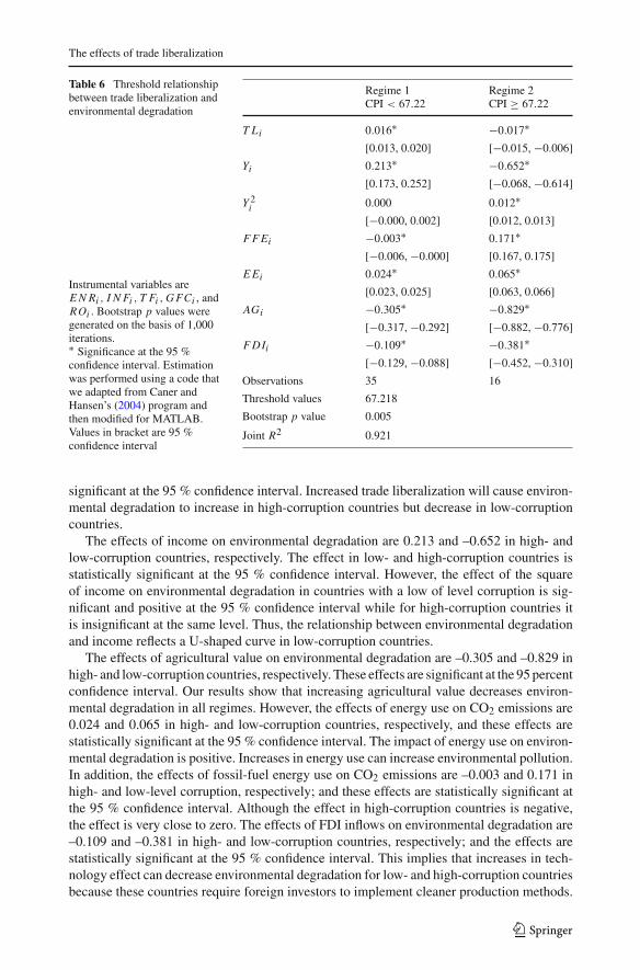
Table 6 Threshold relationshipbetween trade liberalization andenvironmental degradation
Instrumental variables areE N Ri , I N Fi , T Fi , G FCi , andROi . Bootstrap p values weregenerated on the basis of 1,000iterations.∗ Significance at the 95 %confidence interval. Estimationwas performed using a code thatwe adapted from Caner andHansen’s (2004) program andthen modified for MATLAB.Values in bracket are 95 %confidence interval
Regime 1 Regime 2CPI < 67.22 CPI ≥ 67.22
T Li 0.016∗ −0.017∗[0.013, 0.020] [−0.015, −0.006]
Yi 0.213∗ −0.652∗[0.173, 0.252] [−0.068, −0.614]
Y 2i 0.000 0.012∗
[−0.000, 0.002] [0.012, 0.013]
F F Ei −0.003∗ 0.171∗[−0.006, −0.000] [0.167, 0.175]
E Ei 0.024∗ 0.065∗[0.023, 0.025] [0.063, 0.066]
AGi −0.305∗ −0.829∗[−0.317, −0.292] [−0.882, −0.776]
F DIi −0.109∗ −0.381∗[−0.129, −0.088] [−0.452, −0.310]
Observations 35 16
Threshold values 67.218
Bootstrap p value 0.005
Joint R2 0.921
significant at the 95 % confidence interval. Increased trade liberalization will cause environ-mental degradation to increase in high-corruption countries but decrease in low-corruptioncountries.
The effects of income on environmental degradation are 0.213 and –0.652 in high- andlow-corruption countries, respectively. The effect in low- and high-corruption countries isstatistically significant at the 95 % confidence interval. However, the effect of the squareof income on environmental degradation in countries with a low of level corruption is sig-nificant and positive at the 95 % confidence interval while for high-corruption countries itis insignificant at the same level. Thus, the relationship between environmental degradationand income reflects a U-shaped curve in low-corruption countries.
The effects of agricultural value on environmental degradation are –0.305 and –0.829 inhigh- and low-corruption countries, respectively. These effects are significant at the 95 percentconfidence interval. Our results show that increasing agricultural value decreases environ-mental degradation in all regimes. However, the effects of energy use on CO2 emissions are0.024 and 0.065 in high- and low-corruption countries, respectively, and these effects arestatistically significant at the 95 % confidence interval. The impact of energy use on environ-mental degradation is positive. Increases in energy use can increase environmental pollution.In addition, the effects of fossil-fuel energy use on CO2 emissions are –0.003 and 0.171 inhigh- and low-level corruption, respectively; and these effects are statistically significant atthe 95 % confidence interval. Although the effect in high-corruption countries is negative,the effect is very close to zero. The effects of FDI inflows on environmental degradation are–0.109 and –0.381 in high- and low-corruption countries, respectively; and the effects arestatistically significant at the 95 % confidence interval. This implies that increases in tech-nology effect can decrease environmental degradation for low- and high-corruption countriesbecause these countries require foreign investors to implement cleaner production methods.
123
S.-C. Chang
5.4 Robustness tests
Four robustness tests are used to verify our empirical model. The first test verifies whetherour empirical model is goodness of fit and is free of omitted variables. The second testswhether instrumental variables are valid. A weak instrument test developed by Stock andYogo (2005) is used to assess the validity of instrumental variables. The null hypothesis ofa weak instrumental variable is rejected if Cragg–Donald’s Wald statistic is greater than acritical value3 computed by Stock and Yogo (2005). The third tests whether threshold effectsexisted. The fourth checks whether the results presented in the previous subsection are stillvalid if different variables related to governance indicators are treated in turn as the thresholdvariable.
In the first and second robustness tests, this paper estimates five different specifications forthe entire sample of countries without taking into account the possibility of thresholds. Allspecifications have different sets of control variables included in environmental degradation.These control variables include a number of economic factors that are likely to affect CO2
emissions, such as energy use, fossil-fuel energy consumption, and agricultural output. Theresults of these robustness tests are presented in Table 7.
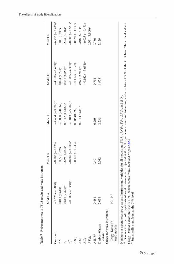
Table 7 summarizes the regression results obtained from various sets of control vari-ables included in Eq. (8). Models A and B have relatively low adjusted R2 values in allspecifications, but Model E has a relatively high adjusted R2 value. This finding verifiesthat Model E is a better fit than the other models. However, in all specifications, trade lib-eralization is found to be statistically insignificant at the 5 % level. Thus, when thresholdeffects are ignored, we are unable to identify any relationship between trade liberalizationand environmental degradation. Table 7 also shows that the null hypothesis of weak instru-ments is rejected at the 5 % significance level. Thus, the instrumental variables are notweak, but strong. This finding verifies the validity of instrumental variables in our empiricalmodel.
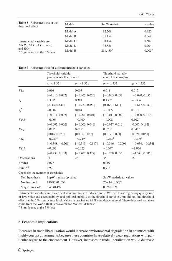
In the third robustness tests, this paper tests whether threshold effects existed in thesefive different model specifications. An approximation of the SupW-statistic and 1,000bootstrap replications are used in threshold test. Table 8 summarizes the results of thresholdeffect obtained from various sets of control variables included in Eq. (9). The comparisonof all model specifications shows that Models A, B, C, and D have no threshold effectat the 5 % significance level, but Model E has a nonlinear effect at the same level. Asthe above discussion shows, the three robustness analyses support the empirical modelof Eq. (9) because Model E is a better fit than the other models and is nonlinear,which is based on the adjusted R-squared value and weak instrument and thresholdtests.
Finally, this paper examines whether the results presented in the previous subsection arestill valid with different threshold variables. Results are reported in Table 9, which shows thatalthough a threshold effect exists at the 5 % significance level when government effectivenessand control of corruption are used as the threshold variables, significant coefficients are few.In addition, this paper tries to use regulatory quality, rule of law, voice and accountability,and political stability as the threshold variables, but results do not indicate threshold effectsat the same level. Thus, our results suggest that other governance indicators are not suitableas the threshold variables, except for CPI.
3 The critical value depends on the number of endogenous variables, number of instruments, and the tolerancefor the “size distortion” of a test (significance level is 5 %).
123
The effects of trade liberalization
Tabl
e7
Rob
ustn
ess
test
inT
SLS
resu
ltsan
dw
eak
inst
rum
ent
Mod
elA
Mod
elB
Mod
elC
Mod
elD
Mod
elE
Con
stan
t−1
.623
(−0.
830)
−0.5
05(−
0.27
3)−4
.404
(−3.
698)
*−4
.018
(−2.
609)
*−6
.835
(−5.
473)
*
TL
i0.
013
(0.6
18)
0.00
5(0
.229
)−0
.008
(−0.
562)
0.02
4(1
.228
)0.
011
(0.9
17)
Y i0.
615
(7.4
25)*
0.63
9(7
.053
)*0.
8147
(11.
187)
*0.
593
(6.8
53)*
0.52
4(6
.716
)*
Y2 i
−0.0
09(−
3.35
0)*
−0.0
09(−
3.38
3)*
−0.0
13(−
5.98
9)*
−0.0
09(−
4.30
7)*
−0.0
06(−
3.62
1)*
FD
I i−0
.128
(−0.
743)
0.00
6(0
.092
)−0
.112
(−1.
177)
−0.0
94(−
1.15
7)
EE
i0.
016
(7.7
23)*
0.02
0(5
.961
)*0.
016
(5.7
61)*
AG
i−0
.162
(−3.
054)
*−0
.023
(−0.
473)
FF
Ei
0.05
1(3
.800
)*
Adj
.R
20.
484
0.49
10.
708
0.71
10.
780
Dur
bin–
Wat
son
stat
istic
2.03
42.
082
2.23
61.
978
2.12
9
Che
ckfo
rw
eak
inst
rum
ent
Cra
gg–D
onal
d’s
Wal
dst
atis
tic10
1.74
+
Num
bers
inpa
rent
hese
sar
ep
valu
es.I
nstr
umen
talv
aria
bles
for
allm
odel
sar
eE
NR
i,IN
Fi,
TF
i,G
FC
i,an
dR
Oi.
+D
enot
esth
atth
enu
llhy
poth
esis
ofw
eak
inst
rum
ents
isre
ject
edat
the
5%
sign
ifica
nce
leve
lan
dto
lera
ting
are
lativ
ebi
asof
5%
ofth
eO
LS
bias
.T
hecr
itica
lva
lue
inC
ragg
–Don
ald’
sW
ald
stat
istic
is13
.97,
whi
chco
mes
from
Stoc
kan
dY
ogo
(200
5)∗ S
tatis
tical
lysi
gnifi
cant
atth
e5
%le
vel
123
S.-C. Chang
Table 8 Robustness test in thethreshold effect
Instrumental variable areE N Ri , I N Fi , T Fi , G FCi ,and ROi∗ Significance at the 5 % level
Models SupW statistic p value
Model A 12.209 0.925
Model B 31.154 0.569
Model C 38.154 0.507
Model D 35.551 0.704
Model E 291.430∗ 0.005∗
Table 9 Robustness test for different threshold variables
Threshold variable:government effectiveness
Threshold variable:control of corruption
qi < 1.321 qi ≥ 1.321 qi < 1.357 qi ≥ 1.357
T Li 0.016 0.003 0.011 0.017
[−0.010, 0.032] [−0.402, 0.026] [−0.005, 0.032] [−0.080, 0.055]
Yi 0.331∗ 0.381 0.433∗ −0.306
[0.116, 0.641] [−0.223, 0.850] [0.163, 0.641] [−0.647, 0.087]
Y 2i −0.002 0.004 −0.005 0.010
[−0.011, 0.002] [−0.001, 0.001] [−0.011, 0.002] [−0.000, 0.019]
F F Ei −0.006 −0.000 −0.008 0.102∗[−0.002, 0.002] [−0.003, 0.046] [−0.027, 0.010] [0.007, 0.162]
E Ei 0.021∗ 0.019∗ 0.020∗ 0.042∗[0.016, 0.023] [0.015, 0.027] [0.017, 0.023] [0.024, 0.051]
AGi −0.289∗ −0.249∗ −0.273∗ −0.349∗[−0.348, −0.209] [−0.313, −0.117] [−0.346, −0.209] [−0.634, −0.234]
F DIi −0.092 −0.025 −0.057 −1.034
[−0.238, 0.103] [−0.407, 0.377] [−0.238, 0.055] [−1.541, 0.305]
Observations 33 26 35 16
p value 0.027 0.002
Joint R2 0.921 0.913
Check for the number of thresholds
Null hypothesis SupW statistic (p value) SupW statistic (p value)
No threshold 130.85 (0.02)* 266.14 (0.00)*
Single threshold 9.48 (0.49) 8.89 (0.82)
Instrumental variables and the critical value see notes of Tables 6 and 7. We tried to use regulatory quality, ruleof law, voice and accountability, and political stability as the threshold variables, but did not find thresholdeffects at the 5 % significance level. Values in bracket are 95 % confidence interval. These threshold variablescome from the World Bank’s “Governance Matters” database∗ Significance at the 5 % level
6 Economic implications
Increases in trade liberalization would increase environmental degradation in countries withhighly corrupt governments because these countries have relatively weak regulations with par-ticular regard to the environment. However, increases in trade liberalization would decrease
123

The effects of trade liberalization
environmental degradation for low-corruption countries because these countries have rel-atively strong legal and political institutions. Along with income growth, the scale of aneconomy tends to become larger and larger. Income growth for high-corruption countriesrequires more input to expand output, but these economic activities will increase emissions.Obviously, pollutant emissions in high-corruption countries are a monotonically increas-ing function of income when the composition effect of economic activity and technologyeffect are controlled for. Hence, rapidly growing developing countries with highly corruptgovernments tend to have high levels of pollution. However, for low-corruption countries,pollutant emissions are a monotonically falling function of income in the same condition.The relationship between environmental degradation and income in low-corruption countriesis a U-shaped curve and does not support the EKC hypothesis. In the U-shaped curve, therelationship between income and environmental degradation trends upward because the con-sumption of dirty goods rises faster than their production (Rothman 1998). Thus, in the longterm, local pollution can be influenced by global pollutants because CO2 is a flow, global,and stock pollutant.
When the scale of an economy and production technologies are constant, scale expansionof agriculture for all countries not only leads to increased agricultural yield in the medium tolong term but also improves air quality. Furthermore, requiring foreign investors to implementcleaner production methods can produce fewer pollutant emissions when the scale of aneconomy and the composition effect of economic activity are constant.
7 Conclusions
The empirical model including trade liberalization, FDI, energy use (e.g., energy use andfossil-fuel energy consumption), and agricultural value is a better fit and is likely to increasethe high explanatory power of estimation because the model has a high adjusted R2 value.Our estimation results confirm that CPI plays a threshold role in the relationship betweenenvironmental conditions and trade liberalization. In addition, the pollution effect of tradeliberalization is nonlinear and has a single-threshold effect. It also provides new evidencethat regime-specific differences are important. The results show that increasing trade liber-alization increases CO2 emissions before a threshold level of corruption has been reached.This implies that environmental degradation is stimulated by trade liberalization for countrieswith high-level corruption. By contrast, increasing trade liberalization reduces CO2 emis-sions after a threshold level of corruption has been reached. This study suggests that furthertrade liberalization and reduced environmental degradation (decline in CO2 emissions) inhigh-corruption countries are competing rather than compatible objectives. On the contrary,further trade liberalization and reduced environmental degradation are compatible rather thancompeting objectives in low-corruption countries.
The hypothesis that a U-shaped relationship between environmental degradation andincome exists in low-corruption countries but is not found in high-corruption countries is sup-ported. The implication of this is that increasing income in low-corruption countries wouldreduce environmental degradation but then increase it after a turning point is reached. How-ever, increasing income in high-corruption countries would increase environmental degrada-tion.
Our results also show that an increase in energy use will increase CO2 emissions inany country. Moreover, holding the scale of an economy constant, increases in agriculturalexpansion and foreign investment can decrease environmental degradation in any country.
123
S.-C. Chang
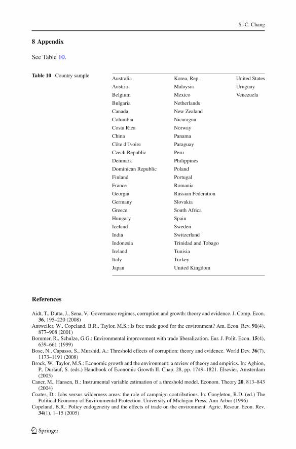
8 Appendix
See Table 10.
Table 10 Country sample Australia Korea, Rep. United States
Austria Malaysia Uruguay
Belgium Mexico Venezuela
Bulgaria Netherlands
Canada New Zealand
Colombia Nicaragua
Costa Rica Norway
China Panama
Côte d’Ivoire Paraguay
Czech Republic Peru
Denmark Philippines
Dominican Republic Poland
Finland Portugal
France Romania
Georgia Russian Federation
Germany Slovakia
Greece South Africa
Hungary Spain
Iceland Sweden
India Switzerland
Indonesia Trinidad and Tobago
Ireland Tunisia
Italy Turkey
Japan United Kingdom
References
Aidt, T., Dutta, J., Sena, V.: Governance regimes, corruption and growth: theory and evidence. J. Comp. Econ.36, 195–220 (2008)
Antweiler, W., Copeland, B.R., Taylor, M.S.: Is free trade good for the environment? Am. Econ. Rev. 91(4),877–908 (2001)
Bommer, R., Schulze, G.G.: Environmental improvement with trade liberalization. Eur. J. Polit. Econ. 15(4),639–661 (1999)
Bose, N., Capasso, S., Murshid, A.: Threshold effects of corruption: theory and evidence. World Dev. 36(7),1173–1191 (2008)
Brock, W., Taylor, M.S.: Economic growth and the environment: a review of theory and empirics. In: Aghion,P., Durlauf, S. (eds.) Handbook of Economic Growth II. Chap. 28, pp. 1749–1821. Elsevier, Amsterdam(2005)
Caner, M., Hansen, B.: Instrumental variable estimation of a threshold model. Econom. Theory 20, 813–843(2004)
Coates, D.: Jobs versus wilderness areas: the role of campaign contributions. In: Congleton, R.D. (ed.) ThePolitical Economy of Environmental Protection. University of Michigan Press, Ann Arbor (1996)
Copeland, B.R.: Policy endogeneity and the effects of trade on the environment. Agric. Resour. Econ. Rev.34(1), 1–15 (2005)
123
The effects of trade liberalization
Copeland, B.R., Taylor, M.S.: Trade, growth, and the environment. J. Econ. Lit. 42(1), 7–71 (2004)Cragg, J.G., Donald, S.G.: Testing identifiability and specification in instrumental variables models. Econom.
Theory 9, 222–240 (1993)Damania, R., Fredriksson, P., List, J.: Trade liberalization, corruption, and environmental policy formation:
Theory and evidence. J. Environ. Econ. Manag. 46(3), 490–512 (2003)Davies, R.B.: Hypothesis testing when a nuisance parameter is present only under the alternative. Biometrika
74, 33–43 (1987)Dean, J.: Does trade liberalization harm the environment? A new test. Can. J. Econ. 35(4), 819–842 (2002)Forslid, R., Okubo, T., Sanctuary, M.: Trade, transboundary pollution and market size, CEPR Discussion
Papers No. 9412, Centre for Economic Policy Research Discussion Papers (2013)Frankel, J.A., Rose, A.K.: Is trade good or bad for the environment? Sorting out the causality. Rev. Econ. Stat.
87(1), 85–91 (2005)Fredriksson, P.G.: The political economy of trade liberalization and environmental policy. South. Econ. J. 65,
513–525 (1999)Gale, L.R., Mendez, J.A.: The empirical relationship between trade, growth and the environment. Int. Rev.
Econ. Finance 7(1), 53–61 (1998)Grossman, G.M., Krueger, A.B.: Environmental impacts of a North American free trade agreement. In: Garber,
P. (ed.) The U.S.-Mexico Free Trade Agreement. MIT Press, Cambridge (1993)Hansen, B.E.: Inference when a nuisance parameter is not identified under the null hypothesis. Econometrica
64, 413–430 (1996)Harbaugh, W.T., Levinson, A., Wilson, D.M.: Reexamining the empirical evidence for an environmental
Kuznets curve. Rev. Econ. Stat. 84(3), 541–551 (2002)Helland, E.: The enforcement of pollution control laws: inspections, violations, and self-reporting. Rev. Econ.
Stat. 80, 141–153 (1998)Hillman, A.L., Ursprung, H.W.: Domestic politics, foreign interests, and international trade policy: reply. Am.
Econ. Rev. 84(5), 1476–1478 (1994)Kwiatkowski, D., Phillips, P.C.B., Schmidt, P., Shin, Y.: Testing the null hypothesis of stationarity against
the alternative of a unit root: how sure are we that economic time series have a unit root? J. Econom. 54,159–178 (1992)
Lai, Y.B.: Interest group, trade liberalization, and environmental standards. J. Environ. Resour. Econ. 34,269–390 (2006)
Lucas, R., Wheeler, D., Hettige, H.: Economic development, environmental regulation and the internationalmigration of toxic international pollution: 1960–1988. In: Low, P. (ed.) International Trade and the Envi-ronment Discussion Paper 159. World Bank, Washington, DC (1992)
Pashigian, B.P.: Environmental regulation: whose self-interests are being protected? Econ. Inq. 23, 551–584(1985)
Philip, P.C.B., Perron, P.: Testing for a unit root in time series regression. Biometrika 75, 335–346 (1988)Rauscher, M.: Environmental regulation and the location of polluting industries, Centre for Economic Policy
Research Discussion Papers No(1032) (1994)Revkin, A.: Warming effects to be widespread. New York Times (2000)Rothman, D.S.: Environmental Kuznets curve—real progress or passing the buck? A case for consumption-
base approaches. Ecol. Econ. 25, 177–194 (1998)Stock, J.H., Yogo, M.: Testing for weak instruments in linear IV regression. In: Andrews, D.W., Stock, J.H.
(eds.) Identification and Inference for Econometric Models: Essays in Honor of Thomas Rothenberg,Chapter 6, pp. 80–108. Cambridge University Press, Cambridge (2005)
Talukdar, D., Meisner, C.M.: Does the private sector help or hurt the environment? Evidence from carbondioxide pollution in developing countries. World Dev. 29(5), 827–840 (2001)
Tamazian, A., Rao, B.B.: Do economic, financial and institutional developments matter for environmentaldegradation? Evidence from transitional economies. Energy Econ. 32(1), 137–145 (2010)
Tamazian, A., Piñeiro, J., Vadlamannati, K.C.: Does higher economic and financial development lead toenvironmental degradation: evidence from BRIC countries. Energy Policy 37(1), 246–253 (2009)
123